Geophysical Evolution of Planetary Interiors and Surfaces: Moon ...

Geophysical Evolution of Planetary Interiors and

Surfaces: Moon & Mars-MASSACHUI

OCT

F r Slt

by

Alexander Joseph Evans

B.S.E., University of Michigan (2006)

Submitted to the Department of Earth, Atmospheric and Planetary Sciencesin partial fulfillment of the requirements for the degree of

Doctor of Philosophy

at the

MASSACHUSETTS INSTITUTE OF TECHNOLOGY

September 2013

@ Massachusetts Institute of Technology 2013. All rights reserved.

/fA uthor ... .. .. .. ... . . . . . C..1... . .. .. . ... .. .....

Deqartment of Earth, Atmospheric and

Certified by ...... . .... ...................

Planetary SciencesSeptember 6, 2013

Maria T. Zuber

72E. A. Griswold Professor of Geophysics

Thesis Supervisor

Accepted by.......- ---- .....Robert D. van der Hilst

Schlumberger Professor of Earth SciencesHead, Department of Earth, Atmospheric and Planetary Sciences

Geophysical Evolution of Planetary Interiors and Surfaces: Moon &

Mars

by

Alexander Joseph Evans

Submitted to the Department of Earth, Atmospheric and Planetary Scienceson September 6, 2013, in partial fulfillment of the

requirements for the degree ofDoctor of Philosophy

Abstract

The interiors and surfaces of the terrestrial planetary bodies provide us a unique opportu-nity to gain insight into planetary evolution, particularly in the early stages subsequent toaccretion. Both Mars and the Moon are characterized by well-preserved and ancient sur-faces, that preserve a record of geological and geophysical processes that have operatedboth at the surface and in the interior. With accessibility to orbital and landed spacecraft,the Moon and Mars have a unique qualitative and quantitative role in understanding andconstraining the evolution of solid planets in our Solar System, as well as the timing of itsmany major events. In this thesis I use gravity and topography data to investigate aspectsof the surface and interior evolution of the Moon and Mars that include aspects of majorprocesses: impact, volcanism, erosion and internal dynamics.

Thesis Supervisor: Maria T. ZuberTitle: E. A. Griswold Professor of Geophysics

3

Acknowledgments

This dissertation would not have been possible without the continuous support I received

from my family, fellow researchers, and friends. I am extremely privileged to have been a

part of the Planetary Geodynamics group at MIT. To my adviser, Professor Maria Zuber, I

am indebted for her continual guidance throughout my six years of graduate school. I am

honored and extremely appreciative for the opportunities that Professor Zuber has extended

to me, along with her other advisees, and I am grateful for her unwavering support of our

individual goals and aspirations.

It has been a truly humbling experience to work alongside such brilliant and hard-working

individuals: Peter James, Mike Sori, Anton Ermakov, ZhenLiang Tian, pilot Frank Cen-

tinello, and Yodit Tewelde. I am especially appreciative for the friendship and mentorship

of my fellow group mates who graduated before me: Dr. Erwan Mazarico, Dr. Ian Garrick-

Bethell, Dr. Wes Watters, and Dr. Sarah Stewart-Johnson.

Also, I am incredibly thankful for my many friends, who without them, I would not have

been able to maintain stability in aspects of my life outside of graduate school. I owe special

thanks to my friend, Dr. Julia Mortyakova for her guidance and emotional support. I could

not imagine going through my graduate experience without the support and friendship of

Dakotta Alex, Brianna Ballard, Jeff Parker, Owen Westbrook, Dr. Anita Ganesan, Dr. Jon

Woodruff, Dr. Oaz Nir, Dr. Kevin McComber, Alejandra Quintanilla Terminel, Ruel Jerry,

Dr. Diane Ivy, Dr. Laura Meredith, Sonia Tikoo, Gabi Melo, Marie Giron, and Sharon

Newman.

I would especially like to thank Dr. Jeffrey Andrews-Hanna and Dr. Jason Soderblom

for their insightful discussions and guidance that helped me grow as a scientist and their

indulgence in my numerous and prolonged unscheduled visits to their office to discuss my

research. I also owe my deepest gratitude to Roberta Allard, Margaret Lankow, and Will

Hodkinson for the many favors and their great problem-solving abilities. Of course, the

opportunities that I have been afforded at MIT would not have been possible without the

financial support from MIT and NASA funding sources.

5

Without qualification, I would like to thank my long-time friends Brian Kitchen and Dr.

Crystal Thrall; I owe you a great many thanks for providing a safe place to complain and a

haven in my spontaneous, yet therapeutic sabbaticals from Boston.

Finally, I would to thank my thesis committee Professors Jeffrey Andrews-Hanna, Tanja

Bosak, Timothy Grove, Taylor Perron, and Maria Zuber for their time, dedication, advice,

and support.

6

Contents

1 Introduction

2 Geophysical Limitations on the Erosion History within Arabia Terra

2.1 Introduction . . . . . . . . . . . . . . . . . . . . . . . . . . . . 2 7

2.2 Methodology . . . . . . . . . . . . . . . . .

2.2.1 Spherical Harmonic Localization . .

2.2.2 Loading Model . . . . . . . . . . . .

2.3 Erosional Constraints within Arabia Terra . .

2.3.1 Terrain and Crustal Thickness . . . .

2.3.2 Gravity . . . . . . . . . . . . . . . .

2.3.3 Estimating Regional Elastic Thickness

2.4 Erosional Scenarios . . . . . . . . . . . . . .

2.4.1 Highlands' Elevation Load . . . . . .

2.4.2 Flexural Fit . . . . . . . . . . . . . .

2.4.3 Uniform Erosion . . . . . . . . . . .

2.4.4 Bounded Erosion . . . . . . . . . . .

2.5 Discussion . . . . . . . . . . . . . . . . . . .

2.6 Conclusions . . . . . . . . . . . . . . . . . .

2.7 Acknowledgements . . . . . . . . . . . . . .

2.8

2.9

Figures . . . . . . . . . . . . . .

Tables . . . . . . . . . . . . . . .

3 A Wet, Heterogenous Lunar Interior: Lower Mantle & Core Dynamo Evolu-

7

23

27

29

29

31

34

34

35

36

38

39

40

42

43

43

46

46

47

56

Introduction ..............

59

. . . . . . . . . . . . . . . . . . 59

3.2 Methodology . . . . . . . . . . . . . . . . . . . . .

3.2.1 Thermochemical Evolution . . . . . . . . . .

3.2.2 Water, Pressure, and Rheology . . . . . . . .

3.2.3 Core Heat Flux & Magnetic Field Intensity .

3.3 Results . . . . . . . . . . . . . . . . . . . . . . . . .

3.3.1 Shallow Lunar Magma Ocean . . . . . . . .

3.3.2 Deep Lunar Magma Ocean . . . . . . . . . .

3.4 Discussion . . . . . . . . . . . . . . . . . . . . . . .

3.5 Summary . . . . . . . . . . . . . . . . . . . . . . .

3.6 Acknowledgements . . . . . . . . . . . . . . . . . .

3.7 Figures . . . . . . . . . . . . . . . . . . . . . . . .

3.8 Tables . . . . . . . . . . . . . . . . . . . . . . . . .

4 A Wet Lunar Mantle: Basin Modification

4.1 Introduction .... ......................

4.2 Methodology

. . . . . . . . . 62

. . . . . . . . . 62

. . . . . . . . . 64

. . . . . . . . . 64

. . . . . . . . . 65

. . . . . . . . . 66

. . . . . . . . . 67

. . . . . . . . . 70

. . . . . . . . . 73

. . . . . . . . . 73

. . . . . . . . . 74

. . . . . . . . . 82

87

......... 87

. . . . . . . . . . . . . . . . . . . . . . . . . . . . . . . . . 8 8

4.2.1 Impact Heating & Initial Basin State . . .

4.2.2 Viscoelastic Relaxation . . . . . . . . . .

Observations & Constraints . . . . . . . . . . . .

Shallow Upper Mantle Water & Basin Relaxation

Results & Discussion . . . . . . . . . . . . . . .

4.5.1 Near-Surface KREEP Layer . . . . . . .

4.5.2 KREEP Component & Water . . . . . .

Sum m ary . . . . . . . . . . . . . . . . . . . . .

Acknowledgements . . . . . . . . . . . . . . . .

Figures . . . . . . . . . . . . . . . . . . . . . .

88

89

90

91

91

92

92

93

93

93

4.9 Tables . . . . . . . . . . . . .

5 Recovery of Buried Lunar Craters

96

99

8

tion

3.1

4.3

4.4

4.5

4.6

4.7

4.8

5.1 Introduction . . . . . . . . . . . . . . . . . . . . .

5.2 Data, Methodology & Modeling . . . . . . . . . .

5.2.1 Spherical Harmonic Localization . . . . .

5.2.2 Gravity Field . . . . . . . . . . . . . . . .

5.2.3 Quasi-Circular Mass Anomaly Identification

5.2.4 Loading Model . . . . . . . . . . . . . . .

5.2.5 Effective Density Estimation . . . . . . . .

5.3 Results & Discussion . . . . . . . . . . . . . . . .

5.3.1 Partially Buried Craters . . . . . . . . . . .

5.3.2 Buried Craters . . . . . . . . . . . . . . .

5.3.3 Surface Depth & Volume Estimates . . . .

5.4 Discussion . . . . . . . . . . . . . . . . . . . . . .

5.4.1 Density . . . . . . . . . . . . . . . . . . .

5.4.2 Mare Depth & Volume . . . . . . . . . . .

5.4.3 Other Factors . . . . . . . . . . . . . . . .

5.5 Summary . . . . . . . . . . . . . . . . . . . . . .

5.6 Acknowledgements . . . . . . . . . . . . . . . . .

5.7 Figures . . . . . . . . . . . . . . . . . . . . . . .

6 Future Work

6.1 A Wet Lunar Mantle: Basin Modification . . . . . . . . . . . . . . . .

6.2 Recovery of Buried Lunar Craters . . . . . . . . . . . . . . . . . . . .

9

. . . . 99

. . . . 100

. . . . 100

. . . . 102

102

. . . . 105

. . . . 105

106

. . . . 106

. . . . 107

. . . . 107

. . . . 109

. . . . 109

. . . . 110

. . . . Ill

. . . . 112

. . . . 112

. . . . 112

125

125

126

List of Figures

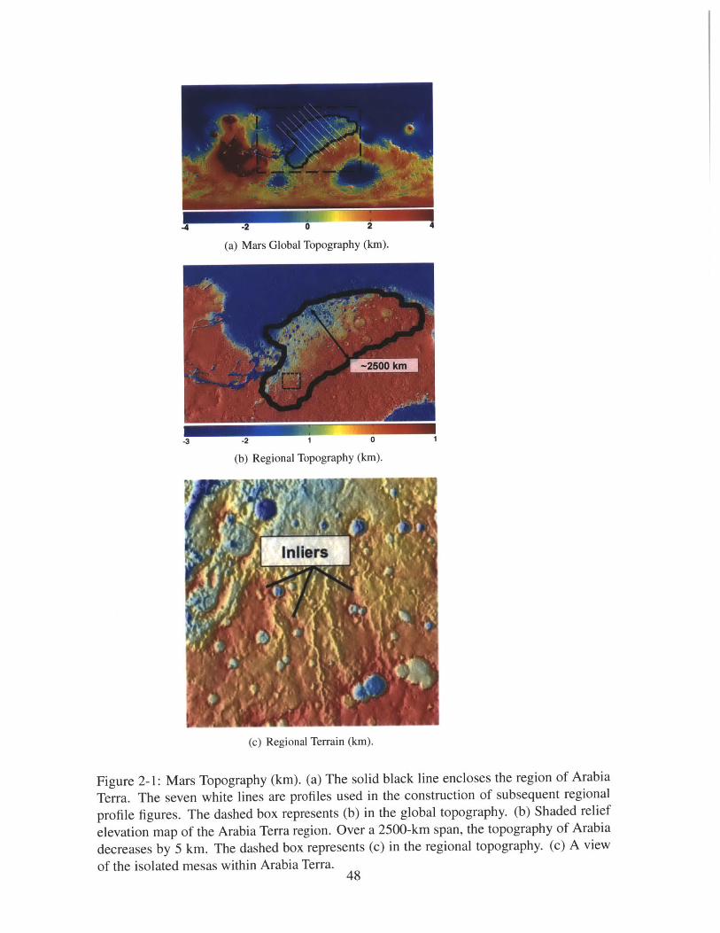
2-1 Mars Topography (km). (a) The solid black line encloses the region of

Arabia Terra. The seven white lines are profiles used in the construction

of subsequent regional profile figures. The dashed box represents (b) in

the global topography. (b) Shaded relief elevation map of the Arabia Terra

region. Over a 2500-km span, the topography of Arabia decreases by 5 km.

The dashed box represents (c) in the regional topography. (c) A view of the

isolated mesas within Arabia Terra . . . . . . . . . . . . . . . . . . . . . . 48

2-2 Mars Crustal Thickness and Gravity Anomaly Maps. (a) Global Crustal

Thickness (km). Within the region of Arabia Terra, the crustal thickness

decreases from 53 km to 28 km near the northern border, yielding a to-

tal crustal thickness reduction of 25 km. The region enclosed by the solid

black line is Arabia Terra. (b) Mars Global Gravity Anomaly (mGal). The

Arabia Terra region is dominated by the antipodal signature associated

with Tharsis. (c) Offset Regional Gravity Anomaly (mGal). A regional

gravity anomaly map with a center-of-mass offset (gi,o =< 18, 0 > and

g1,1 =< 43, -144 > of the gravity field, gim) incorporated to offset the

antipodal signature associated with Tharsis. . . . . . . . . . . . . . . . . . 49

11

2-3 (a) Admittance Minimum Misfit. The admittance for Arabia Terra is best

fit by a model with an elastic thickness of 15 km, denoted in the misfit

by the asterisk. The misfit is applied between degrees 20 through 50. (b)

Model and Observation Admittance. The model admittance is shown above

for an elastic lithosphere thickness of 5 km (circles), 15 km (solid), 30

km (dashed-dotted), 45 km (dotted), and 60 km (dashed). The thick line

represents the actual free-air admittance for Arabia Terra. The peak in

admittance near degree-18 is due to long-wavelength effects (e.g., Tharsis).

(c) Coherence. The thick line represents the coherence for Arabia Terra and

the thin line represents the theoretical coherence for an elastic lithosphere

of 15km. .... ....... ............................... 50

2-4 Conceptual Model. Extending left to right from the southern highlands

to the northern lowlands, respectively, the conceptual model illustrates a

crustal cross-section along the Arabia Terra dichotomy boundary. The

dark-shaded region represents the present-day crustal thickness and ele-

vation of Arabia Terra. The dashed lines represent the pre-erosional state

of Arabia Terra with a highlands-like elevation and crustal thickness. The

light-shaded region represents the eroded amount for each scenario. (a)

Highlands' Elevation Load. The erosional load is the spatially-varying el-

evation difference between the mean southern highlands' elevation (pre-

erosional Arabia Terra and the present-day Arabia Terra elevation. (b)

Flexural Fit. The erosional load (superimposed on present-day topography)

is designed to match the observed elevation of Arabia Terra by accounting

for flexure. Significantly more erosion is required than in the Highlands'

Elevation Load. . . . . . . . . . . . . . . . . . . . . . . . . . . . . . . . . 51

12

2-5 Highlands' Elevation Load. (a) Erosional Load (km). Load applied to

Arabia Terra region. The erosional load is the spatially-varying elevation

difference between the mean southern highlands' elevation and the Arabia

Terra elevation. (b) Deflection (km). Resultant flexure from erosional load.

(c) Gravity Anomaly (mGal). The model gravity anomaly map of Arabia

Terra after the erosion. The resultant gravity anomaly includes the finite

amplitude effect resulting from topography on the surface and along the

crust-mantle boundary. . . . . . . . . . . . . . . . . . . . . . . . . . . . . 52

2-6 Averaged Profiles for Formational Erosion Scenarios. The profiles ex-

tend from the southern highlands to the northern lowlands as shown in

Figure 2-1(a). The distance from the southern highlands is on the hori-

zontal axis. The unshaded regions contain data internal to Arabia Terra.

The light-shaded regions incorporate data interior and exterior to Arabia

Terra, while the dark-shaded region represents data solely exterior to Ara-

bia Terra. Shown above are model data of the Flexural Fit scenario (thin

solid), the Highlands' Elevation Load scenario (dashed-dotted), and the

observation data (thick solid) along with the standard deviation (dotted)

of Arabia Terra. (a) Elevation (km). The final topography of the forma-

tional erosion scenarios, referenced to a 2100 m elevation, are shown with

the present-day elevation of the region. The averaged profile for the Flex-

ural Fit scenario matches the present-day Arabia Terra elevation, unlike

the Highlands' Elevation Load. (b) Crustal Thickness (km). The present-

day crustal thickness of Arabia Terra is matched by the Flexural Fit sce-

nario within the region, unlike the Highlands' Elevation Load scenario. (c)

Gravity Anomaly (mGal). The observed relative gravity anomaly (exte-

rior gravity anomaly less the interior gravity anomaly) is exceeded by both

formational erosion scenarios. . . . . . . . . . . . . . . . . . . . . . . . . 53

13

2-7 Flexural Fit Scenario. (a) Erosional Load (km). Load applied to Arabia

Terra region. The erosional load is designed to match the observed eleva-

tion of Arabia Terra. (b) Deflection (km). Resultant flexure from erosional

load. (c) Gravity Anomaly (mGal). The model gravity anomaly map of

Arabia Terra after the erosion. The resultant gravity anomaly includes the

finite amplitude effect resulting from topography on the surface and along

the crust-mantle boundary. . . . . . . . . . . . . . . . . . . . . . . . . . . 54

2-8 Averaged Profiles for Non-Formational Erosion Scenarios. The profiles

extend from the southern highlands to the northern lowlands as shown in

Figure 2-1(a). The distance from the southern highlands is on the hori-

zontal axis. The unshaded regions contain data internal to Arabia Terra.

The light-shaded regions incorporate data interior and exterior to Arabia

Terra, while the dark-shaded region represents data solely exterior to Ara-

bia Terra. (a) Maximum Bounded Erosional Load (km). The offset of the

present-day topography from the initial topography (solid line) is shown

along with the erosion load (dashed-dotted line) and the deflection (dashed

line). (b) Maximum Uniform Erosional Load (km). The offset of the

present-day topography from the initial topography (solid line) is shown

along with the 1300-m uniform erosional load (dashed-dotted line) and the

deflection (dashed line). (c) Gravity Anomaly (mGal). Averaged profile

of gravity anomaly for 450-m erosional load (solid line), maximum uni-

form erosional load (dashed line), and the maximum bounded erosional

load (dashed-dotted line). . . . . . . . . . . . . . . . . . . . . . . . . . . . 55

3-1 Initial temperature and density profiles used in our convective models with

ATcmb = 200 K. Shown is the temperature profile of the deep LMO sce-

nario (blue solid line) as determined by (1) compared to the shallow LMO

(red dashed line). . . . . . . . . . . . . . . . . . . . . . . . . . . . . . . . 75

14

3-2 CMB heat fluxes for shallow lunar magma ocean model. The CMB heat

flux (blue solid line) is shown on the left axis with the minimum heat flux

needed to sustain a core dynamo (red dash-dot line) and the core tempera-

ture (black dashed line) on the right axis. (a, b, c) Models with (ATemb =

0 K). (d, e, f) Models with ATemb = 200 K. (a) Case ZXXO1: No Water

Enrichment, (b) case ZXX02: 200-km water-enriched layer with 40±20

ppm water, (c) Case ZXX03: 500-km water-enriched layer with 40±20

ppm water, (d) Case ZXX25: No Water Enrichment, and (e) Case ZXX26:

200-km water-enriched. . . . . . . . . . . . . . . . . . . . . . . . . . . . . 76

3-3 Temperatures and CMB heat fluxes for shallow lunar magma ocean model

with ATemb = lOOK. (a,d) Case ZXX25: No Water Enrichment, (b,e) Case

ZXX26: 200-km water-enriched layer with 40+20 ppm water, and (c,f)

Case ZXX27: 500-km water-enriched layer with 40±20 ppm water. (b, c)

Mantle temperature differences relative to the non water-enriched scenario

for water-enriched models. In (d,e,f) CMB Heat Flux (blue solid line) as

a function of model start time is shown on the left axis with the minimum

heat flux needed to sustain a core dynamo (red dash-dot line) and the core

temperature (black dashed line) on the right axis. . . . . . . . . . . . . . . 77

3-4 Half-Hemisphere temperature view of the lunar mantle model. ATe,1b =

0 K. Shown are lunar interior panels with pseudocolor temperature (K) at

0.25, 0.50, and 1.0 Gyr after model initialization. a, b, c) Case VXX07 (no

water enrichment). (d, e, f) ase VXX08 (200-km water-enriched layer with

40±20 ppm water). (g, h, i) Temperature difference between cases VXX08

and VXX07, highlighting the increased convection vigor of the water-rich

layer. The radial average of the temperature difference with time is shown

in Figure 3-5b . . . . . . . . . . . . . . . . . . . . . . . . . . . . . . . . . 78

15

3-5 Temperatures and heat fluxes for deep lunar magma ocean model with

A Tmb =0 K. (a,d) Case VXX07: No Water Enrichment, (b,e) Case VXX08:

200-km water-enriched layer with 40±20 ppm water, (c,f) Case VXX09:

500-km water-enriched layer with 40±20 ppm water, The radially-averaged

temperature in time is shown for Case ZXXO1 in panel (a) with panels (b,c)

tracking the temperature differences with time relative to Case VXX07. In

(d, e, f), the CMB heat flux (blue solid line) is shown on the left axis with

the minimum heat flux needed to sustain a core dynamo (red dash-dot line)

and the core temperature (black dashed line) on the right axis. . . . . . . . 79

3-6 CMB heat fluxes for deep lunar magma ocean model. The CMB heat

flux (blue solid line) is shown on the left axis with the minimum heat flux

needed to sustain a core dynamo (red dash-dot line) and the core tempera-

ture (black dashed line) on the right axis. (a, b, c) Models with (ATeflb =

100K) Case VXX37: No Water Enrichment, Case VXX38: 200-km water-

enriched layer with 40±20 ppm water, and Case VXX39: 500-km water-

enriched layer with 40±20 ppm water, respectively. (d, e, f) Models with

(A Tenb = 200K) Case VX43: No Water Enrichment, Case VX44: 200-

km water-enriched layer with 40±20 ppm water, and Case VX45: 500-km

water-enriched layer with 40±20 ppm water. . . . . . . . . . . . . . . . . 80

16

3-7 Temperatures and CMB heat fluxes for case for the temperature-damped,

deep lunar magma ocean model with ATmb = 0 K. (a,d) Case VXX13:

350-km core radius and no water enrichment, (b,e) Case VXX14: 350-km

core radius and 200-km water-enriched layer with 40±20 ppm water, (c)

Case VX13: 450-km core radius and no water enrichment, (f) Case VX14:

450-km core radius and 200-km water-enriched layer with 40±20 ppm wa-

ter. The temperature evolution in model time is shown with radius for Case

VXX 13 in panel (a) with panel (b) showing the temperature difference of

Case VXX14 at the same time relative to Case VXX13. In c-f the CMB

heat flux (blue solid line) is shown on the left axis with the minimum heat

flux needed to sustain a core dynamo (red dash-dot line) and the core tem-

perature (black dashed line) on the right axis. . . . . . . . . . . . . . . . . 81

4-1 Basin Depth Normalized to Initial Basin Center Depth (Cases with varying

KREEP content). Present-day depth of basins including the effect of sub-

crustal KREEP concentration of 100% (blue) is compared with scenario

without a sub-crustal KREEP component (green). . . . . . . . . . . . . . . 94

4-2 Basin Depth Normalized to Initial Basin Center Depth (Cases with Wa-

ter and KREEP). Present-day depth of basins with water concentrations at

varying radial positions of 1690 km (dash-dotted line) and 1670 km (dashed

line). The reference (solid lines) are relaxation curves with no water for a

sub-crustal KREEP concentration of 50% (green) and with no sub-crustal

KREEP (blue). . . . . . . . . . . . . . . . . . . . . . . . . . . . . . . . . 95

5-1 Lunar Nearside Gravity. Superimposed craters (black) and quasi-circular

mass anomalies (magenta) are shown on the lunar nearside a) Bouguer

anomaly and b) modified antieigenvalue maps. . . . . . . . . . . . . . . . . 113

17

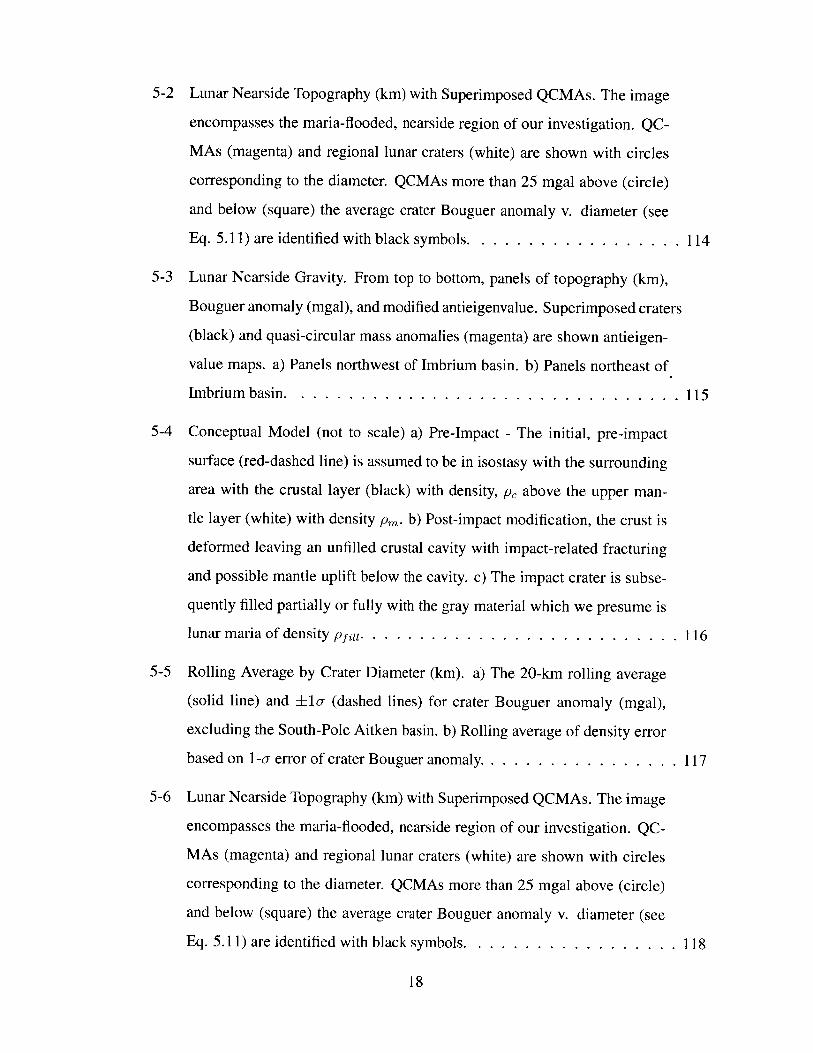
5-2 Lunar Nearside Topography (km) with Superimposed QCMAs. The image

encompasses the maria-flooded, nearside region of our investigation. QC-

MAs (magenta) and regional lunar craters (white) are shown with circles

corresponding to the diameter. QCMAs more than 25 mgal above (circle)

and below (square) the average crater Bouguer anomaly v. diameter (see

Eq. 5.11) are identified with black symbols. . . . . . . . . . . . . . . . . . 114

5-3 Lunar Nearside Gravity. From top to bottom, panels of topography (km),

Bouguer anomaly (mgal), and modified antieigenvalue. Superimposed craters

(black) and quasi-circular mass anomalies (magenta) are shown antieigen-

value maps. a) Panels northwest of Imbrium basin. b) Panels northeast of

Im brium basin. . . . . . . . . . . . . . . . . . . . . . . . . . . . . . . . . 115

5-4 Conceptual Model (not to scale) a) Pre-Impact - The initial, pre-impact

surface (red-dashed line) is assumed to be in isostasy with the surrounding

area with the crustal layer (black) with density, pc above the upper man-

tle layer (white) with density pm. b) Post-impact modification, the crust is

deformed leaving an unfilled crustal cavity with impact-related fracturing

and possible mantle uplift below the cavity. c) The impact crater is subse-

quently filled partially or fully with the gray material which we presume is

lunar maria of density pfi. . . . . . . . . . . . . . . . . . . . . . . . . . . 116

5-5 Rolling Average by Crater Diameter (km). a) The 20-km rolling average

(solid line) and +lo- (dashed lines) for crater Bouguer anomaly (mgal),

excluding the South-Pole Aitken basin. b) Rolling average of density error

based on 1-- error of crater Bouguer anomaly. . . . . . . . . . . . . . . . . 117

5-6 Lunar Nearside Topography (km) with Superimposed QCMAs. The image

encompasses the maria-flooded, nearside region of our investigation. QC-

MAs (magenta) and regional lunar craters (white) are shown with circles

corresponding to the diameter. QCMAs more than 25 mgal above (circle)

and below (square) the average crater Bouguer anomaly v. diameter (see

Eq. 5.11) are identified with black symbols. . . . . . . . . . . . . . . . . . 118

18

5-7 Partially-Buried Craters Densities using GRAIL Data. a). The density

contrast between the infill density and the excavated (pre-impact surface)

density for the excess material in partially buried crater. b) Crater count

for partially-buried craters with the calculated excavated density. c) Crater

count for partially-buried craters with the calculated density contrast be-

tween the infill density and the excavated density. d) Crater count for

partially-buried craters across infill density. . . . . . . . . . . . . . . . . . 119

5-8 QCMA Trends using GRAIL Data. a) Normalized Average Bouguer Anomaly

(mgal) v. Diameter (km). Assuming the QCMAs are buried craters, gravity

anomaly is reference to the gravity anomaly within the ejecta blanket area.

QCMAs (magenta circles) and lunar crater catalog (black dots) are shown

with circles corresponding to diameter. QCMAs more than 25 mgal above

(blue asterisks) and below (green asterisks) the normalized average crater

Bouguer anomaly v. diameter. The lines are from Equation 5.17 with den-

sity contrasts of -200 (red-dashed), 0 (red solid), 200 (cyan dashed), 400

(cyan solid), 600 (cyan dashed-dot), and 800 (red dashed-dot) kg/m3 . b)

Crater Count v Density Contrast (kg/m3 ). The density contrast between the

infill density and the excavated (pre-impact surface) density for the excess

material in partially buried crater. . . . . . . . . . . . . . . . . . . . . . . 120

5-9 Nearside Mare Fill Depth Estimates (km). (a) Maximum Depth. This

scenario is calculated based on interpolated differences of regional craters

depths to reference fresh crater depths. (b) Completely and Partially Buried

Crater Depth. This scenario is calculated based on interpolated differences

of completely and partially buried craters depths to reference fresh crater

depths. (c) Completely Buried Crater Rim Height and Partially Buried

Crater Depths. This scenario is calculated based on completely buried

crater rim heights and partially buried craters depths to reference fresh

crater depths. . . . . . . . . . . . . . . . . . . . . . . . . . . . . . . . . . 121

19

5-10 Effective Density Model. Using Equation 5.19, we calculate the theoreti-

cal profile for density contrast of 500 and -500 kg/m 3 at a depth of 6 km.

A positive density contrast (denser material below surface) yields a repre-

sentative monotonically decreasing curve and a negative density contrast

(denser material layer at surface) yields a representative monotonically in-

creasing curve. . . . . . . . . . . . . . . . . . . . . . . . . . . . . . . . . 122

5-11 Localized Admittance (90 spherical cap) for Non-Mare Region. Localized

admittance curves for spherical cap centered at (a) 00, 60"N and (b) 8'E,

62"N. The decreasing effective density trend between harmonic degrees

250-600 indicate a layer of decreasing density at the surface. With a range

of density contrasts (1400 - 200 kg/m 3) and subsurface densities (1500 -

2800 kg/m 3), we use Equation 5.19 to calculate the count of best-fit depths

(within 30% of minimum misfit) for regions (c) 0', 601N and (d) 8"E, 62'N. 123

5-12 Localized Admittance (90 spherical cap) for Mare Region. Localized ad-

mittance curves for spherical cap centered at (a) 40"E, 460 N and (b) 0",

50"N. Increasing effective density trend between harmonic degrees 250-

600 indicate a layer of increased density at the surface. With a range

of density contrasts (1400 - 200 kg/M 3) and subsurface densities (1500 -

2800 kg/m 3), we use Equation 5.19 to calculate the count of best-fit depths

(within 30% of minimum misfit) for regions (c) 40"E, 460N and (d) 00, 50"N. 124

20

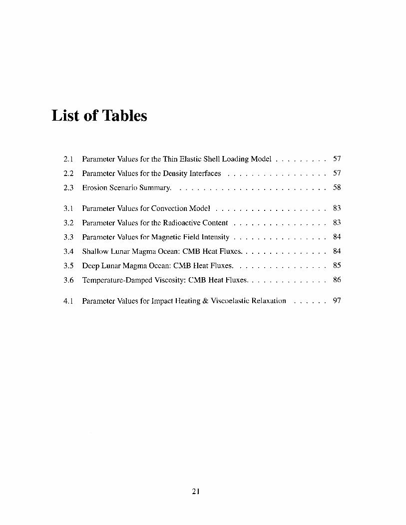
List of Tables

2.1 Parameter Values for the Thin Elastic Shell Loading Model . . . . . . . . . 57

2.2 Parameter Values for the Density Interfaces . . . . . . . . . . . . . . . . . 57

2.3 Erosion Scenario Summary. . . . . . . . . . . . . . . . . . . . . . . . . . 58

3.1 Parameter Values for Convection Model . . . . . . . . . . . . . . . . . . . 83

3.2 Parameter Values for the Radioactive Content . . . . . . . . . . . . . . . . 83

3.3 Parameter Values for Magnetic Field Intensity . . . . . . . . . . . . . . . . 84

3.4 Shallow Lunar Magma Ocean: CMB Heat Fluxes. . . . . . . . . . . . . . . 84

3.5 Deep Lunar Magma Ocean: CMB Heat Fluxes. . . . . . . . . . . . . . . . 85

3.6 Temperature-Damped Viscosity: CMB Heat Fluxes. . . . . . . . . . . . . . 86

4.1 Parameter Values for Impact Heating & Viscoelastic Relaxation . . . . . . 97

21

Chapter 1

Introduction

For most of history, humans gazed upward to the great unknown and wondered what mys-

teries lie beyond. Over four centuries ago, pioneers of the scientific revolution such as

Galileo Galilei and Sir Isaac Newton embarked on the arduous task of unraveling the mys-

teries of the Universe. Now, over 400 years later, with spacecraft, new technologies, and

the capability to send humans into space, the arduous task of unraveling the mysteries of

the Universe continues. In this thesis, I examine a few of the many current mysteries and

attempt to provide a unique perspective on unanswered questions within the inner Solar

System.

Starting with the ancient terrain of Arabia Terra region of Mars, an area of -1 x 107 km2

lying south of the hemispheric dichotomy boundary, I use altimetry data returned by the

Mars Orbiter Laser Altimeter (MOLA) on the Mars Global Surveyor (MGS) along with

gravity data from the Mars Reconnaissance Orbiter (MRO) to constrain the volume of ma-

terial removed by aqueous and aeolian processes. Constraining material removed from this

unique physiographic province, which possesses topography and crustal thickness interme-

diate between those of the southern highlands and northern lowlands, will provide insight

into the formation of the Martian hemispheric topographic and crustal dichotomy. I em-

ploy a multi-taper, spatio-spectral localization approach to gravity-topography admittance

estimates and find a best-fit elastic thickness estimate that may be used to constrain surface

23

loading in the region. I find the elevation difference between Arabia Terra and the south-

ern highlands would require up to 25-km erosion in order to reproduce the elevation and

crustal thickness deficit of Arabia Terra. Such a large amount of erosion would result in

exterior flexural uplift surpassing 1 km and gravity anomalies exceeding observations by

-60 mGal. Consequently, it is unlikely that Arabia Terra was formed from surface erosion

alone. I determine that no more than 3 x 107 km3 of material could have been removed from

Arabia Terra, while 1.7 x 108 km3 of erosion is required to explain the observed crustal

thickness.

Given the canonical model of lunar formation from a giant impact of a Mars-sized body

with the Earth, understanding the evolution of the Moon has direct consequences for Earth.

Recent re-analyses of Apollo-era lunar samples indicate the Moon contained regions with

water concentrations of at least 260 ppm in the deep lunar interior prior to 3 billion years

ago and the Moon had a convective core dynamo from at least 4.2-3.56 billion years ago

(Gya). Past investigations of lunar convective dynamos with a generally homogeneous and

relatively dry Moon have been unable to yield adequate heat flux at the core-mantle bound-

ary to sustain core convection for such a long time. Using a finite-element model, I inves-

tigate the possible consequences of a heterogeneously wet and compositionally stratified

lunar interior for the evolution of the lunar mantle. I find that a compositionally-stratified

mantle could result in a core heat flux sufficiently high to sustain a dynamo through 2.4

Ga and a maximum surface magnetic field strength of 5.1 pT. Further, I find that if water

was transported or retained preferentially in the deep interior, even in small amounts (<20

ppm), it would have played a significant role in transporting heat out of the deep interior

and reducing the lower mantle temperature. Thus, water, if enriched in the lower mantle,

could have influenced core dynamo timing by up to 1.0 billion years (Gyr) and enhanced

the vigor of a lunar core dynamo. My results demonstrate the plausibility of a convective

lunar core dynamo even beyond the period currently indicated by the Apollo samples. Near

the surface, a water-enriched region of the Moon that retains a non-negligible portion of

radioactive material at the base of the crust could diminish the surface expression of im-

pact basins in excess of 30% via viscoelastic relaxation. Without a near-surface radioactive

material layer, water alone may have caused non-negligible relaxation of surface features

24

older than 4.1 Gya.

With newly acquired data by the dual Gravity Recovery and Interior Laboratory (GRAIL)

spacecraft, I find over 100 quasi-circular mass anomalies on the lava-flooded region of

the Moon. As impact craters are the most ubiquitous circular features on the Moon, I

interpret these mass anomalies as gravity signatures of buried impact craters. I use this

buried crater population to investigate the thickness, volume, and density of cooled lava

(basalt) emplaced on the lunar nearside. My analyses suggest that nearside lunar basalts

have a density contrast of 800 kg/m3 relative to the lunar crust and at least 2 x 107 km3 of

basalt was emplaced on the lunar surface. The existence of such a large quantity of buried

craters indicates that there is a heterogeneous distribution of lunar basalt across the lunar

nearside, with craters and rims requiring burial by more than 5 km of basalt. In concert with

80 anomalously shallow lunar nearside craters, I find the lunar maria may have a density

contrast of 800 kg/m 3 with the anorthositic highlands crust, indicating an average density

of lunar maria 3300±200 kg/m3

With this thesis, I hereby contribute the results of my investigations to the body of knowl-

edge for the formation and evolution of our Solar System and the Universe.

25

Chapter 2

Geophysical Limitations on the Erosion

History within Arabia Terra

This chapter has been published and can be referenced as: Evans, A. J., Andrews-Hanna,

J. C., & Zuber M. T (2010). Geophysical limitations on the erosion history within Arabia

Terra. Journal of Geophysical Research-Planets, 115(E5). doi:10.1029/2009JE003469.

Copyright 2010 by the American Geophysical Union. 0148-0227/10/2009JE003469.

2.1 Introduction

Arabia Terra, with an area of I x 107 km2 centered at (25E, 5N), is an anomalous region

along the Martian dichotomy boundary. Traditionally considered part of the ancient south-

ern highlands (e.g., (2; 3; 4; 5)), Arabia Terra provides a more gradual transition from the

southern highlands to the northern lowlands in both topography (6; 7) and crustal thick-

ness (8; 9). While the geological processes leading to the formation of the region have

not been clearly identified (e.g., (10)), Arabia Terra contains morphological evidence in-

dicative of surface erosion including isolated mesas (11; 12) and partially degraded craters

(13). Though surface modification has been suggested for the entirety of the highlands (e.g.,

(14)), the anomalous nature of Arabia Terra and its geomorphology may indicate preferen-

27

tial erosion of the region. The amount of erosion may have generated a significant volume

of sediment, possibly contributing to the resurfacing of the northern lowlands.

Though previous workers have attempted to constrain the amount of erosion for Arabia

Terra and the southern highlands in general, much of the analyses have been based on crater

degradation with anywhere between 200 m to 2300 m of material being eroded, as put forth

by (14). (11) approached the problem from an alternative geomorphic perspective: using

the height of local elevation maxima (isolated mesas) in concert with the mapping of geo-

logical units. Their analysis indicates that a minimum of 1000 m of material was removed

from the Arabia Terra region in the late Noachian. Recent analysis of data from the Mars

Exploration Rover landing site at Meridiani Planum within Arabia Terra suggests smaller

amounts of erosion have occurred since -3.0 Ga, though evidence for this erosion is found

on sedimentary deposits that lie above the original surface and thus does not constitute

net loss (15). It has generally been suggested that erosion during the Noachian and early-

mid Hesperian may have been greater due to a warmer and wetter environment (14; 15).

Widespread layered deposits across the region suggest an early period of deposition as well

(16; 17).

Prior analyses of erosion in Arabia Terra (e.g., (11)) relied on the geomorphology of the

terrain and craters. In this paper, we present our constraints for the erosion of Arabia Terra

based on geodynamical modeling coupled with limitations established from topography

and gravity data returned by the Mar Orbiter Laser Altimeter (MOLA) (18; 6) on the Mars

Global Surveyor (MGS) (19) and the gravity field investigation on the Mars Reconnais-

sance Orbiter (MRO) (20), respectively. By comparing the expected flexural response and

gravitational signature (21) of various erosional loads to the observational data, we estab-

lish an upper limit on the amount of material that could have been removed from within

Arabia Terra. We employ a lithospheric flexure model to attain the flexural rebound and

gravitational signature associated with a given erosional load. Exploiting recent advances

in spherical harmonic localization techniques (22; 23), we better constrain the elastic litho-

sphere thickness (24) - a crucial parameter in resolving the flexural response to erosion.

Our flexure model, based upon the thin elastic shell method of (21), estimates the mem-

28

brane and bending stresses for a load supported by an elastic lithosphere underlain by a

fluid-like medium. We test the viability of several erosional scenarios, including loads ca-

pable of reproducing the unique topography and crustal structure of Arabia Terra from an

initial, highlands-like terrain.

2.2 Methodology

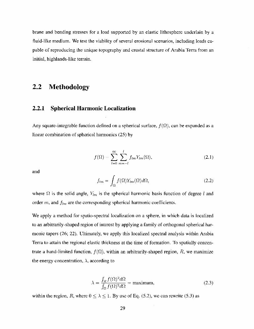
2.2.1 Spherical Harmonic Localization

Any square-integrable function defined on a spherical surface, f(Q), can be expanded as a

linear combination of spherical harmonics (25) by

00 1

f (Q) = E E fim Y1mn(Q), (2.1)1=0 m=-1

and

firn = f (Q)Ym(Q)dQ, (2.2)

where Q is the solid angle, Ym is the spherical harmonic basis function of degree I and

order m, and fim are the corresponding spherical harmonic coefficients.

We apply a method for spatio-spectral localization on a sphere, in which data is localized

to an arbitrarily-shaped region of interest by applying a family of orthogonal spherical har-

monic tapers (26; 22). Ultimately, we apply this localized spectral analysis within Arabia

Terra to attain the regional elastic thickness at the time of formation. To spatially concen-

trate a band-limited function, f(Q), within an arbitrarily-shaped region, R, we maximize

the energy concentration, A, according to

A R f(Q) 2 dQ - maximum, (2.3)f0 f(Q) 2 dQ

within the region, R, where 0 < A < 1. By use of Eq. (5.2), we can rewrite (5.3) as

29

Lai. 1 Lwin it

Z E fim E E Dim' m'fi'mf

A 0 m=-l L11=0 m'=-1'

Sfi21=0 m=-1

where

Dimim = j YiM(Q)Ymi(Q) dQ, (2.5)

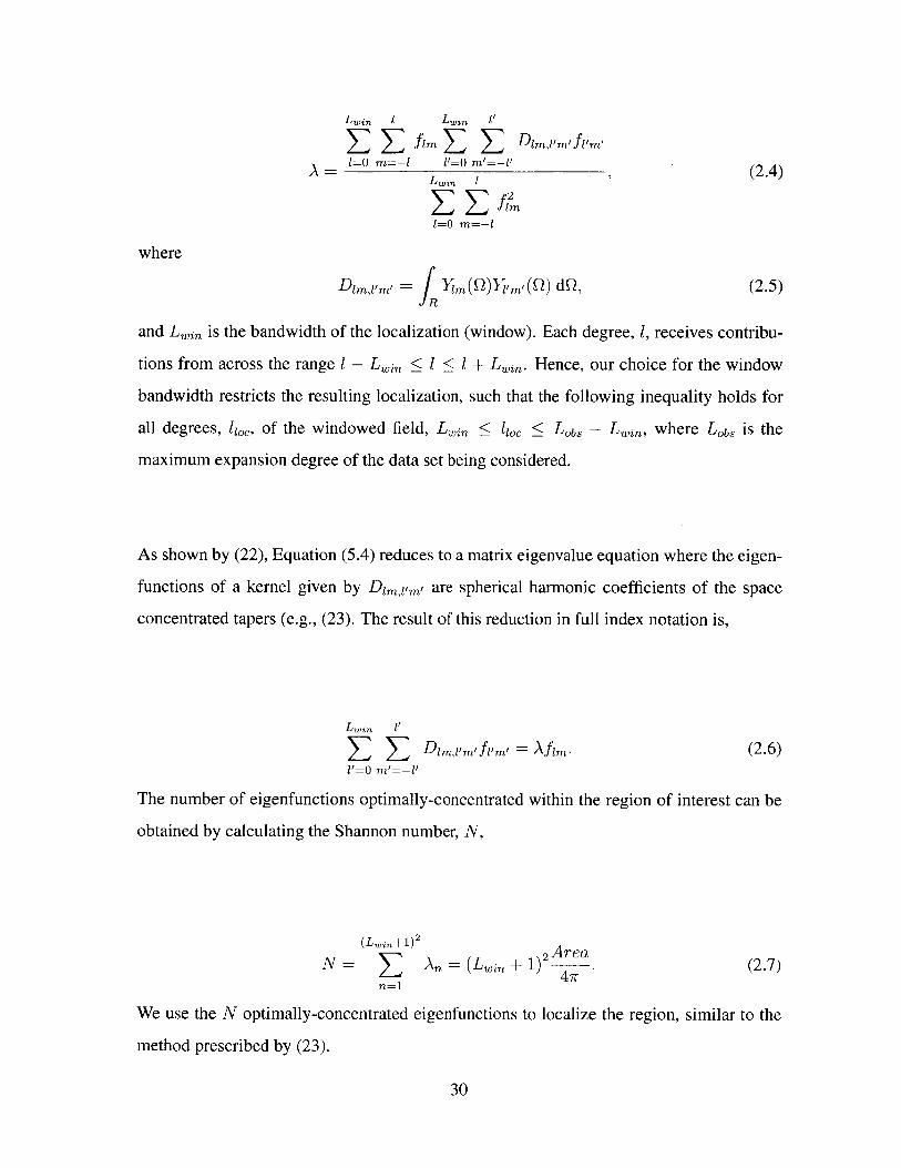
and Lin is the bandwidth of the localization (window). Each degree, 1, receives contribu-

tions from across the range 1 - Lwin 1 + Lwin. Hence, our choice for the window

bandwidth restricts the resulting localization, such that the following inequality holds for

all degrees, 11, of the windowed field, Lin < 11oc < Lob, - Lwin, where Lob, is the

maximum expansion degree of the data set being considered.

As shown by (22), Equation (5.4) reduces to a matrix eigenvalue equation where the eigen-

functions of a kernel given by Dimpm, are spherical harmonic coefficients of the space

concentrated tapers (e.g., (23). The result of this reduction in full index notation is,

Lwin if

E E Dirnirfi'm = Afim. (2.6)1'=0 m'=-l'

The number of eigenfunctions optimally-concentrated within the region of interest can be

obtained by calculating the Shannon number, N,

(Lein +1)2

N An = (Lwin + 1) . (2.7)47

n=1

We use the N optimally-concentrated eigenfunctions to localize the region, similar to the

method prescribed by (23).

30

2.2.2 Loading Model

Thin Elastic Shell Adaptation

In order to represent the effects of erosion in Arabia Terra, we account for the resultant

flexure and gravity signature of the erosional load. We establish limits on the extent of

regional erosion by analyzing these resultant signatures and comparing to observational

data.

We employ an adapted version (27) of the thin elastic lithosphere (shell) model outlined by

(21). Following (21), we introduce the dimensionless parameters,

ETeE e =(2.8)

R 2 gAp

andD

(2.9)R 4 g~p'

where E is Young's modulus, Te is the elastic lithosphere thickness at the time of loading,

R is the mean radius of the shell, g is the Martian gravitational acceleration, and Ap is the

density contrast between continua below and above the shell. The mean shell radius, R, and

flexural rigidity, D, can be represented as R = Rp - Te/2 and D = ET,3/12(1 - V2), where

v is Poisson's ratio and Rp is the equatorial planetary radius. The independent parameters

that we use for the loading model are listed in Table 2.1.

We use spherical harmonic representations of the load thickness h, the resulting deflection

w, and the equipotentially-referenced, final topography h. Relating the load thickness and

flexure in the spectral domain yields the relationship,

Wim = L 1 hl, (2.10)

where PL is the load (crustal) density and the transfer function,

31

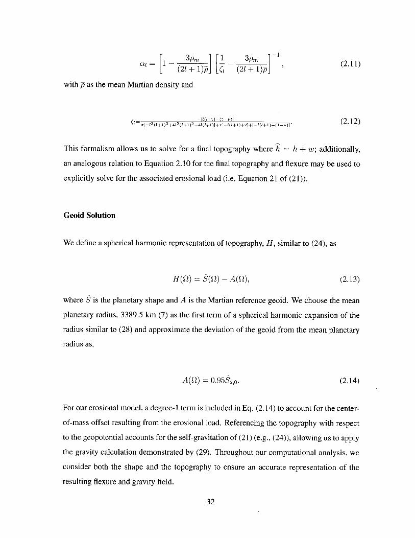
a = I - 3 p, 1 _ __ (2.11)1 (21 + I)1) 1 (21 + 1)P_ '

with p as the mean Martian density and

-lui1)-( -- )](2.12)- l--13(1+1)3

+412

(l+1)2

-41(l+1)]+r-1(l+1)+21+[-1(1+1)+(1-v)]

This formalism allows us to solve for a final topography where h = h + w; additionally,

an analogous relation to Equation 2.10 for the final topography and flexure may be used to

explicitly solve for the associated erosional load (i.e. Equation 21 of (21)).

Geoid Solution

We define a spherical harmonic representation of topography, H, similar to (24), as

H(Q) = $(Q) - A(Q), (2.13)

where S is the planetary shape and A is the Martian reference geoid. We choose the mean

planetary radius, 3389.5 km (7) as the first term of a spherical harmonic expansion of the

radius similar to (28) and approximate the deviation of the geoid from the mean planetary

radius as,

A(Q) = 0.95S 2,0 . (2.14)

For our erosional model, a degree- 1 term is included in Eq. (2.14) to account for the center-

of-mass offset resulting from the erosional load. Referencing the topography with respect

to the geopotential accounts for the self-gravitation of (21) (e.g., (24)), allowing us to apply

the gravity calculation demonstrated by (29). Throughout our computational analysis, we

consider both the shape and the topography to ensure an accurate representation. of the

resulting flexure and gravity field.

32

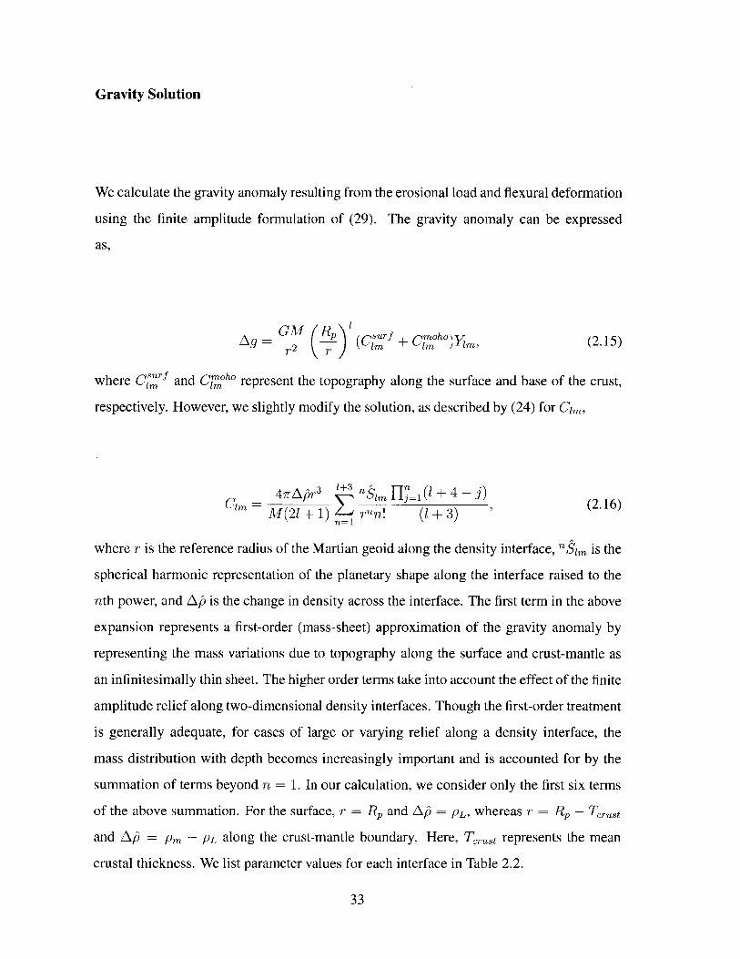
Gravity Solution

We calculate the gravity anomaly resulting from the erosional load and flexural deformation

using the finite amplitude formulation of (29). The gravity anomaly can be expressed

as,

GM(R'\'g =g (Cf' + CM"Oo)Ylm, (2.15)

r r (i

where C7'.'f and Coho represent the topography along the surface and base of the crust,

respectively. However, we slightly modify the solution, as described by (24) for Cim,

4ira1r 3 ' 3 fl+imFs=1 + 4-)Cim = M2n1 _ (1±3 ) (2.16)

M(21 + 1) n=1 ! (1 +3) '

where r is the reference radius of the Martian geoid along the density interface, "Sim is the

spherical harmonic representation of the planetary shape along the interface raised to the

nth power, and Ay is the change in density across the interface. The first term in the above

expansion represents a first-order (mass-sheet) approximation of the gravity anomaly by

representing the mass variations due to topography along the surface and crust-mantle as

an infinitesimally thin sheet. The higher order terms take into account the effect of the finite

amplitude relief along two-dimensional density interfaces. Though the first-order treatment

is generally adequate, for cases of large or varying relief along a density interface, the

mass distribution with depth becomes increasingly important and is accounted for by the

summation of terms beyond n = 1. In our calculation, we consider only the first six terms

of the above summation. For the surface, r = Rp and A = PL, whereas r = Rp - Tcrust

and A = Pm - PL along the crust-mantle boundary. Here, Trust represents the mean

crustal thickness. We list parameter values for each interface in Table 2.2.

33

2.3 Erosional Constraints within Arabia Terra

Using altimetry data returned by the MOLA (18; 6) on MGS (19) along with gravity data

from MRO (20), we place geophysical constraints on the maximum amount of erosion for

Arabia Terra. We analyze the topography (7) and gravity (30) in a 10 resolution grid in the

spatial domain. Unless otherwise noted, we expand our data fields to I = 75. We define

and restrict our investigation of Arabia Terra to the region outlined by Figure 2-1(a). Here,

we examine the unique structure of Arabia Terra and key evidence interpreted as erosional

indicators.

2.3.1 Terrain and Crustal Thickness

The elevation (6; 7) and crustal thickness (8; 9) profiles within Arabia Terra decrease

gradually to the north, in between more discrete transitions at the northern and southern

boundaries of the province (31). The topography decreases by -5 km over a distance of

2500 km across Arabia Terra (Figure 2-1(b)), while the crustal thickness decreases by

~25 km. Unlike other areas along the Martian dichotomy boundary, Arabia Terra is af-

forded a more gentle transition from the highlands to the northern lowlands in elevation

and crustal thickness as shown in Figure 2-2(a) (6; 7). Though the region possesses to-

pography and crustal thickness that are arguably more similar to the northern lowlands (8),

recent analysis by (31) reveals the northern edge of Arabia Terra is continuous with the

crustal dichotomy boundary, suggesting that Arabia Terra is, in a physiographic sense, part

of the highlands.

Arabia Terra contains many inliers (local elevation maxima) and isolated mesas (fretted

terrain) that have been interpreted as evidence for a prior, more elevated surface (e.g., (11;

32). In order to gauge the minimal amount of eroded material, (11) use the local elevation

maxima to establish a lower bound on regional erosion. (11) restricted their investigation

to western Arabia Terra and Margaritifer Sinus and estimated a minimum of 4.5 x 106

km3 of eroded material. If distributed across Arabia Terra, this total amount of erosion is

equivalent to a uniform erosional load of 450 m.

34

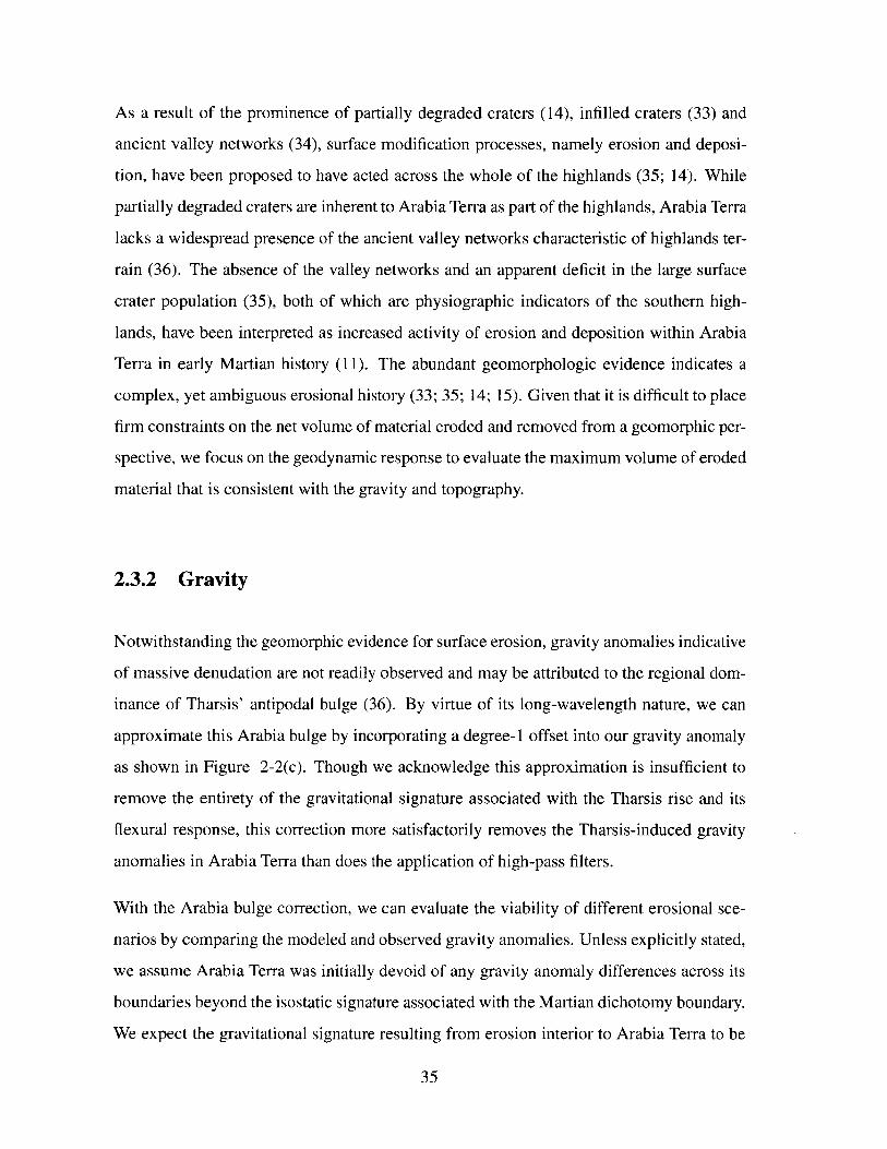
As a result of the prominence of partially degraded craters (14), infilled craters (33) and

ancient valley networks (34), surface modification processes, namely erosion and deposi-

tion, have been proposed to have acted across the whole of the highlands (35; 14). While

partially degraded craters are inherent to Arabia Terra as part of the highlands, Arabia Terra

lacks a widespread presence of the ancient valley networks characteristic of highlands ter-

rain (36). The absence of the valley networks and an apparent deficit in the large surface

crater population (35), both of which are physiographic indicators of the southern high-

lands, have been interpreted as increased activity of erosion and deposition within Arabia

Terra in early Martian history (11). The abundant geomorphologic evidence indicates a

complex, yet ambiguous erosional history (33; 35; 14; 15). Given that it is difficult to place

firm constraints on the net volume of material eroded and removed from a geomorphic per-

spective, we focus on the geodynamic response to evaluate the maximum volume of eroded

material that is consistent with the gravity and topography.

2.3.2 Gravity

Notwithstanding the geomorphic evidence for surface erosion, gravity anomalies indicative

of massive denudation are not readily observed and may be attributed to the regional dom-

inance of Tharsis' antipodal bulge (36). By virtue of its long-wavelength nature, we can

approximate this Arabia bulge by incorporating a degree-I offset into our gravity anomaly

as shown in Figure 2-2(c). Though we acknowledge this approximation is insufficient to

remove the entirety of the gravitational signature associated with the Tharsis rise and its

flexural response, this correction more satisfactorily removes the Tharsis-induced gravity

anomalies in Arabia Terra than does the application of high-pass filters.

With the Arabia bulge correction, we can evaluate the viability of different erosional sce-

narios by comparing the modeled and observed gravity anomalies. Unless explicitly stated,

we assume Arabia Terra was initially devoid of any gravity anomaly differences across its

boundaries beyond the isostatic signature associated with the Martian dichotomy boundary.

We expect the gravitational signature resulting from erosion interior to Arabia Terra to be

35

observable as a change across the northern and southern provincial boundaries. We define

this gravity anomaly difference between the exterior and interior of Arabia Terra as the

relative gravity anomaly (RGA).

Accordingly, we focus our comparison on analyzing the relative gravity anomaly across

the boundaries. We use the average gravity anomaly and standard error on the mean (noise

measurement) to establish a limit of 4+2 milligals (mGal) for the relative gravity anomaly

along the southern boundary of Arabia Terra. In northern Arabia Terra, we observe a

strong negative gravity anomaly immediately exterior to the boundary. Relative to Arabia

Terra, this highly localized signal provides for a negative relative gravity anomaly across

the northern boundary, whereas an Arabia Terra erosional load would generate a positive

relative gravity anomaly at the boundary. This anomaly could not have been generated

by an erosional load interior to Arabia Terra and could conceivably be a result of crustal

flow along the dichotomy boundary (37), (31). As a result, we contrast the interior gravity

anomaly with its exterior counterpart beyond this highly localized signature to attain a

16±4-mGal relative gravity anomaly along the northern boundary.

We use the constraints of 6 mGal and 20 mGal for the maximum relative gravity anomalies

for the southern highlands and northern lowlands, respectively.

2.3.3 Estimating Regional Elastic Thickness

Admittance & Coherence

In order to model the geophysical response to erosion within Arabia Terra, we must first

constrain the elastic thickness at the time of the erosion. The free-air admittance relation is

used to place limits on the effective elastic thickness for a given region (38). Over geologic

timescales, the effective response of the Martian lithosphere to a surface load can be well

approximated by an elastic plate with a specified elastic thickness, Te. For thin elastic shell

loading, Equations (2.8 -2.16) provide a linear mapping between the applied load and the

gravity anomaly (27), neglecting finite amplitude effects. The transfer function relating the

36

final topography to the gravity anomaly is primarily sensitive to the elastic thickness and

not the magnitude of the load.

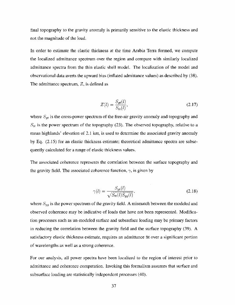
In order to estimate the elastic thickness at the time Arabia Terra formed, we compute

the localized admittance spectrum over the region and compare with similarly localized

admittance spectra from the thin elastic shell model. The localization of the model and

observational data averts the upward bias (inflated admittance values) as described by (38).

The admittance spectrum, Z, is defined as

__Sgt (1 )Z(l) = (2.17)

Set(l)'

where Sgt is the cross-power spectrum of the free-air gravity anomaly and topography and

Set is the power spectrum of the topography (23). The observed topography, relative to a

mean highlands' elevation of 2.1 km, is used to determine the associated gravity anomaly

by Eq. (2.15) for an elastic thickness estimate; theoretical admittance spectra are subse-

quently calculated for a range of elastic thickness values.

The associated coherence represents the correlation between the surface topography and

the gravity field. The associated coherence function, -y, is given by

Sgt (l )= ,() (2.18)

/Stt () )S9 (1 )

where Sgg is the power spectrum of the gravity field. A mismatch between the modeled and

observed coherence may be indicative of loads that have not been represented. Modifica-

tion processes such as un-modeled surface and subsurface loading may be primary factors

in reducing the correlation between the gravity field and the surface topography (39). A

satisfactory elastic thickness estimate, requires an admittance fit over a significant portion

of wavelengths as well as a strong coherence.

For our analysis, all power spectra have been localized to the region of interest prior to

admittance and coherence computation. Invoking this formalism assumes that surface and

subsurface loading are statistically independent processes (40).

37

Results

Since the elastic thickness in Eqns. (2.8) and (2.9) is a sensitive parameter with respect

to the permissible erosional load and is poorly constrained for Arabia Terra, we utilize the

free-air gravity admittance to attain a better estimate. We identify the best-fit elastic thick-

ness of Te=15 km by minimizing the misfit (Figure 2-3(a)) between modeled and observed

admittances. As we choose L,,i=15, the localized admittance can only be computed for

degrees 15 through 60, limited by the finite bandwidth of our spatio-spectral localization.

As shown in Figure 2-3(b), this provides a reasonable fit between degrees 20 and 50,

though the observed admittance takes a downturn beyond degree 50. The local maximum

at degree 18 is a distortion by the long-wavelength effects of the rotational flattening and

Tharsis, since degree-18 in the localized data includes contributions from as low as degree-

3 in the global data fields. Notwithstanding this aberration in the admittance, an elastic

thickness of 15 km provides a best fit between degrees 20 and 50.

For any region with accurately modeled loads, we expect a coherence near unity for all

degrees (39). In the presence of noise, un-modeled surface loads, or sub-surface loading,

the coherence may decrease. Though we restrict our investigation to only surface loading,

the lesser values in the observed coherence also suggest that other processes - subsurface

erosion or generation of crustal density anomalies - may have acted within Arabia Terra.

Even so, the coherence (Figure 2-3(c)) remains relatively high for the localized region

which indicates that if subsurface erosion did occur, it is not a significant influence on the

regional gravitational anomaly.

2.4 Erosional Scenarios

We focus on four main erosional scenarios for the province of Arabia Terra:

1. Highlands' Elevation Load - an erosional load of the spatially-varying, present-

day elevation difference between the mean southern highlands' elevation and Arabia

Terra.

38

2. Flexural Fit - an erosional load yielding the current surface elevation of Arabia Terra

after flexural adjustment.

3. Uniform - a uniformly thick layer of erosion applied to the whole of Arabia Terra.

4. Bounded - a linearly-interpolated load with erosional constraints at the northern and

southern provincial boundaries.

We employ a forward modeling approach to thoroughly examine each of the aforemen-

tioned loading scenarios for Arabia Terra. For each scenario, the erosion is represented as

a removal of a surface load with a uniform density of 2900 kg m- (8; 24). Though we

acknowledge that other cases which partially erode a sub-region of Arabia Terra may be

equally valid, for simplicity, we constrain our study to scenarios which erode the whole

of Arabia Terra. The material eroded in these scenarios is assumed to have been removed

entirely from the region.

2.4.1 Highlands' Elevation Load

The Highlands' Elevation Load (Figure 2-4(a)) represents the present-day elevation dif-

ference of Arabia Terra from the mean highlands' elevation of 2100 m. In this scenario,

we investigate the viability of forming Arabia Terra from highlands-like terrain and crustal

thickness by removing a load representative of the present-day elevation difference. The

erosional load ranges from 0 to 5100 m in thickness (Figure 2-5(a)). We contrast this

scenario with the Flexural Fit scenario to quantify the importance of flexure. Along with

the assumption of an initial 2100-m elevation for Arabia Terra, we assume that the basic

physical properties of the highlands are the same as those within Arabia Terra.

Applying the Highlands' Elevation Load to the thin elastic shell model results in a final

topography that does not yield present-day Arabia Terra (Figure 2-6(a)). We disregard the

sharp transition at the northern and southern edges as a result of spherical harmonic ringing

inherent in such a model.

The flexural rebound (deflection) generates significant uplift (Figure 2-5(b)), yielding a

39

region with an elevation that decreases by 700 m from the southern to the northern boundary

of Arabia Terra. This produces a final topography with an elevation trend shallower than

the current Arabia Terra and deviates from the observed elevation at the northern boundary

by over 4 km. As illustrated in Figure 2-6(a), the flexural rebound also generates 500 m of

uplift exterior to the northern boundary. This 500-m uplift exterior to northern Arabia Terra

lies outside of one standard deviation of the regional elevation profile. Additionally, the

amount of erosion does not achieve the deficit required to match the observed reduction in

regional crustal thickness (Figure 2-6(b)). Thus, the crustal thickness and the topography,

interior and exterior to Arabia Terra, fail to match the observations.

Although the relative gravity anomaly along the southern boundary is small at 8 mGal, it

still exceeds the 6-mGal limit imposed by the observations. Larger amounts of erosion at

the northern boundary result in a greater relative gravity anomaly of 20 mGal, consistent

with the maximum allowable RGA identified for northern Arabia Terra.

While this erosional scenario is nearly consistent with the observed gravity anomalies,

it cannot reproduce the present-day topography or crustal thickness of the region. The

inability of this scenario to yield an elevation consistent with the current state of Arabia

Terra demonstrates the importance of flexure. The topography of Arabia Terra cannot be

reproduced without significantly more erosion than calculated by the elevation difference

alone. Hence, this erosional scenario cannot be singularly responsible for the formation of

Arabia Terra.

2.4.2 Flexural Fit

Incorporating flexure into the reconstruction of the original surface requires erosion of a

significantly greater amount (Figure 2-4(b)) than the prior scenario. We employ an analo-

gous relation to Equation 2.10, as previously discussed, to permit an explicit calculation of

the amount of additional erosion required to produce the present-day Arabia Terra topogra-

phy. The supposition of erosion as the primary mechanism responsible for the current phys-

iographic state of Arabia Terra requires the initial (pre-erosion) elevation to be coincident

40

with the southern highlands' elevation of 2100 m, similar to the previous scenario.

The erosional load required to form the topography of Arabia Terra from an initial state

similar to the southern highlands is shown in Figure 2-7(a). The amount of erosion is

equivalent to a 750-m layer of sediment spread across the whole of the northern lowlands.

With a 15-km elastic thickness, this scenario erodes up to 22 km at the northern extremity

yielding a total eroded volume of 1.7 x 108 km3 . This erosional load reproduces the crustal

thickness deficit (Figure 2-6(b)) to within 5 km of Arabia Terra relative to the southern

highlands.

As a consequence of erosional amounts in excess of the elastic (lithosphere) thickness, we

invoke the caveat that the erosion must transpire on a timescale sufficiently long to allow

for thermal diffusion to maintain a minimal elastic thickness of 15 km. Using the thermal

diffusion timescale, the erosion must occur in no less than 2.4 My or at a rate less than 9.2

mm/yr. This rate is orders of magnitude greater than the average erosion rates estimated

for Mars (14), justifying the assumption of a minimal elastic thickness during the erosional

event.

Though the erosional load is designed to reproduce the topographic expression of Arabia

Terra, the scenario fails to reproduce the elevation exterior to Arabia Terra and an allowable

relative gravity anomaly. In eroding nearly 22 km at the northern extremity, the resultant

flexural rebound produces uplift of over 1 km immediately exterior to Arabia Terra. This

substantial elevation rise is contradictory to the observations and is too large to be masked

by measurement noise. While this 1-km exterior uplift alone is sufficient to deem this sce-

nario implausible, the resultant gravitational anomaly further diminishes the viability of

this scenario. The gravity anomaly map in Figure 2-7(c) contains an 80-mGal relative

gravity anomaly across the northern boundary, 60 mGal greater than allowable for north-

ern Arabia Terra. Furthermore, this scenario establishes a strong gradient in the gravity

anomaly interior to Arabia Terra, contradictory to observations of a nearly uniform gravity

anomaly. The relative gravity anomaly on the southern boundary of 40 mGal also surpasses

the allowable RGA of 6 mGal.

Though the relative gravity anomalies are too large to be accommodated by the observa-

41

tions, the resulting crustal thickness trend more closely resembles crustal thickness models

than the prior scenario. While the discrepancy in crustal thickness in the erosional model is

small, the overcompensated, excess crustal thickness is sufficient to produce large negative

gravity anomalies over Arabia Terra, in conflict with the observations.

This scenario is designed to reproduce the topography of Arabia Terra via erosion from

an initial state similar to the southern highlands. Using this scenario, we produce an over-

compensated Arabia Terra crustal thickness estimate with a gravity anomaly trend inte-

rior to Arabia Terra and relative gravity anomalies on the northern and southern bound-

aries that exceed the observations. Thus, these results demonstrate that erosion cannot

be solely responsible for the formation of the current Arabia Terra from a highlands-like

elevation.

2.4.3 Uniform Erosion

This scenario diverges from the notion of a pre-erosional Arabia Terra commensurate with

the southern highlands and instead erodes a uniformly thick layer from Arabia Terra. In

order to yield a final elevation and crustal thickness consistent with the current state of

Arabia Terra, the pre-erosional state includes isostatic crustal thickness variations specific

to the applied erosional load.

As the gravity anomalies arising from isostatically compensated topography are small rel-

ative to those arising from flexurally supported loads, the uniform erosion scenario will

produce a similar relative gravity anomaly across all boundaries. We first consider an

amount of erosion consistent with (11), a uniform erosional load of 450 m. This erosional

load produces a 3-mGal and 2-mGal relative gravity anomaly on the northern and southern

boundaries, respectively (Figure 2-8(c)). The amount of flexural rebound immediately ex-

terior to Arabia Terra is minimal. Accordingly, this amount of erosion is allowable based

on the observations.

Using an iterative, forward-modeling approach to minimize the misfit between the modeled

and observed relative gravity anomalies, we can determine the maximum amount of uni-

42

form erosion consistent with the observations. The 6-mGal relative gravity anomaly on the

southern boundary is the primary constraint, allowing for a maximum uniform erosional

load (Figure 2-8(a)) of approximately 1300 m. Neglecting contributions to the south-

ern RGA from noise/error, a best-fit uniform erosional load can also be determined: 750

m.

2.4.4 Bounded Erosion

The difference in the observed northern and southern RGA upper limit suggests that a rel-

atively larger amount of erosion is allowable along the northern boundary. In this scenario,

we consider a load with assigned erosional amounts on each boundary; between the bound-

aries, the erosion is linearly interpolated to attain the erosional load.

Through an iterative forward-modeling scheme similar to the prior scenario, we determine

the maximum amount of erosion for Arabia Terra (Figure 2-8(b)) - erosion linearly in-

creases from 300 m in the south and culminates at 5000 m in the north. This maximum

erosional load attains the 6-mGal and 20-mGal relative gravity anomaly upper limit along

the southern and northern boundaries, respectively. Thus, this bounded erosional load is

compatible with the upper bound of the relative gravity anomalies along the boundaries.

This maximum erosional load amounts to 3.1 x 107 km3 of material that could have con-

ceivably been removed from Arabia Terra. Additionally, we calculate a best-fit bounded

erosional load designed to match the observed northern and southern RGA without error.

The best-fit bounded erosional load increases from no erosion in the south to 4000 m in the

north.

2.5 Discussion

The thin elastic shell loading model applied here provides constraints on the maximum

volume of erosion which can reproduce the observed gravity anomalies (Table 2.3). In

addressing erosion from the vantage of geophysics, we eliminate uncertainty in the inter-

43

pretation of geological units and employ a model independent of specific fluvial or aeo-

lian processes. Our 15-km elastic thickness is consistent with past estimates for north-

eastern Arabia Terra and the bulk of the southern highlands (T < 16 km) (24; 41). In

general, the southern highlands have a lower elastic thickness than the more rigid low-

lands, yielding more intermediate elastic thickness estimates along the dichotomy bound-

ary (24; 41; 8; 42; 43; 44; 45).

Any significant alteration of Arabia Terra would have likely occurred prior to the onset

of the Hesperian epoch in order to maintain current estimates for the terrain age (13) and

to be consistent with the thin elastic thickness (24). It is likely that if erosion did occur

within Arabia Terra, it may have occurred over a period of time (15; 11; 14) rather than

in a single event. As our admittance and coherence analysis indicates, Arabia Terra was

formed in the presence of a 15-km elastic lithosphere; any subsequent surface modification

would have occurred at a greater elastic thickness. Since the lithosphere becomes more

rigid over time (i.e. the elastic thickness increases), a given erosional load will result in

a larger relative gravity anomaly. Therefore, by modeling erosion with a 15-km elastic

lithosphere, the viable erosional loads likely represent an upper limit for erosion within

Arabia Terra.

As illustrated by the Highlands' Elevation Load, the Arabia Terra topography cannot be

reproduced by the removal of a load representative of the elevation difference as a result of

subsequent flexural rebound. Although we can reproduce the topography of Arabia Terra

via the Flexural Fit scenario, the erosion required produces large gravity anomalies and

lowlands' uplift in conflict with the observations. Further, the removal of massive amounts

of material would have likely generated large surface stresses and tectonic features contrary

to regional observations (46; 47).

Although the current physiographic expression of Arabia Terra cannot be explained by

erosion, lesser amounts of erosion are allowable within the region from the geodynami-

cal constraints. Employing a fit to the relative gravity anomaly of Arabia Terra, uniform

erosion of no greater than 1300 m of material could have occurred; beyond 1300 m, the rel-

ative gravity anomaly along the southern boundary of the province is exceeded. However,

44

the larger relative gravity anomaly in northern Arabia Terra allows for a greater amount of

material to have been removed. Accordingly, our bounded erosional load can reproduce

the difference between the maximum allowable relative gravity anomalies. The erosional

load linearly increases with distance from the southern boundary of Arabia Terra with 300

m of erosion in the south and up to 5000 m in the north. The load represents the maximum

amount that may be removed from Arabia Terra: 3 x 107 km3 of material. Though this load

is consistent with the gravity observations, it cannot produce the Arabia Terra topography

or crustal structure from highlands-like topography or crustal thickness.

Given the constraint on the surface age from crater statistics, a majority of the erosion

from the Highlands Flexural Fit scenario would have had to occur no later than -3.8

Ga. Though lateral crustal flow may have diminished the resultant gravity anomalies ob-

served on present-day Mars, the persistence of the north-south crustal dichotomy boundary

through the early Noachian provides a constraint on crustal relaxation (8; 48; 37; 49). On

the basis of thermal models that include consideration of crustal heat production and the

role of hydrothermal circulation in the crust, relaxation rates <10-17 1s- required to main-

tain crustal thickness variations are achieved (49). The relaxation rate constraint is easily

met for plausible thermal structures in the Noachian, and limits vertical perturbation of

the crust-mantle boundary to be on the order of 1 km within Arabia Terra. Thus, while

crustal flow within Arabia Terra would affect our estimate on the maximum amount of

erosion, erosion with crustal flow still cannot explain the formation of Arabia Terra from

the southern highlands. Further, it is likely crustal-thinning resulting from erosion would

increase the effective viscosity allowing for greater preservation of the Arabia Terra crustal

profile (37; 8). Ultimately, given the assumption of a pre-erosional Arabia Terra similar to

the highlands, the preservation of the large-scale Noachian crustal thickness variations on

Mars (i.e. crustal dichotomy boundary, Hellas) suggests that lower crustal flow would not

have been substantial within Arabia Terra (37).

45

2.6 Conclusions

In order for erosion to be a viable candidate for the formation of Arabia Terra from highlands-

like topography and crustal thickness, an erosional model must reproduce the topography

and gravity anomaly both within and exterior to the region. Appropriately reproducing the

topography entails the consideration of flexure; without the consideration of flexure the

load itself cannot properly be determined or evaluated.

Our admittance analysis demonstrates that the present-day topography of Arabia Terra was

established in the presence of a 15-km elastic lithosphere. This lithosphere thickness de-

termines the flexural response of Arabia Terra to any large-scale loading event. In order to

generate via erosion the observed topography of Arabia Terra from highlands-like topog-

raphy and crustal thickness, 1.7 x 10' km3 of material must be eroded from the region.

However, this erosion would result in a substantial flexural uplift of the lithosphere imme-

diately exterior to Arabia Terra and resultant gravity anomalies that exceed observations by

~60 mGal.

This work demonstrates the maximum amount of erosion that could have occurred in Ara-

bia Terra is 3 x 107 km3, consistent with the geological minimum established by (11). Fur-

ther, we conclude that either some other mechanism (e.g., (31)) removed crust from Arabia

Terra thereby dominating the regional evolution or alternatively the region developed with

less topography and a thinner crust relative to the rest of the southern highlands. If the

unique physiography of this region is a result of erosion, it must have been accompanied

by significant viscous relaxation (37) or must have possessed large isostatic crustal thick-

ness variations prior to erosion. Ultimately, erosion alone cannot explain the observed

topography and crustal thickness deficit of Arabia Terra.

2.7 Acknowledgements

I thank Jeff Andrews-Hanna for guidance and support in developing models and research

approach and I think F. Simons for assistance in spherical harmonic localization.

46

2.8 Figures

47

(a) Mars Global Topography (kn).

-3 -2 1 U

(b) Regional Topography (kin).

(c) Regional Terrain (kin).

Figure 2-1: Mars Topography (km). (a) The solid black line encloses the region of Arabia

Terra. The seven white lines are profiles used in the construction of subsequent regional

profile figures. The dashed box represents (b) in the global topography. (b) Shaded relief

elevation map of the Arabia Terra region. Over a 2500-km span, the topography of Arabia

decreases by 5 km. The dashed box represents (c) in the regional topography. (c) A view

of the isolated mesas within Arabia Terra.48

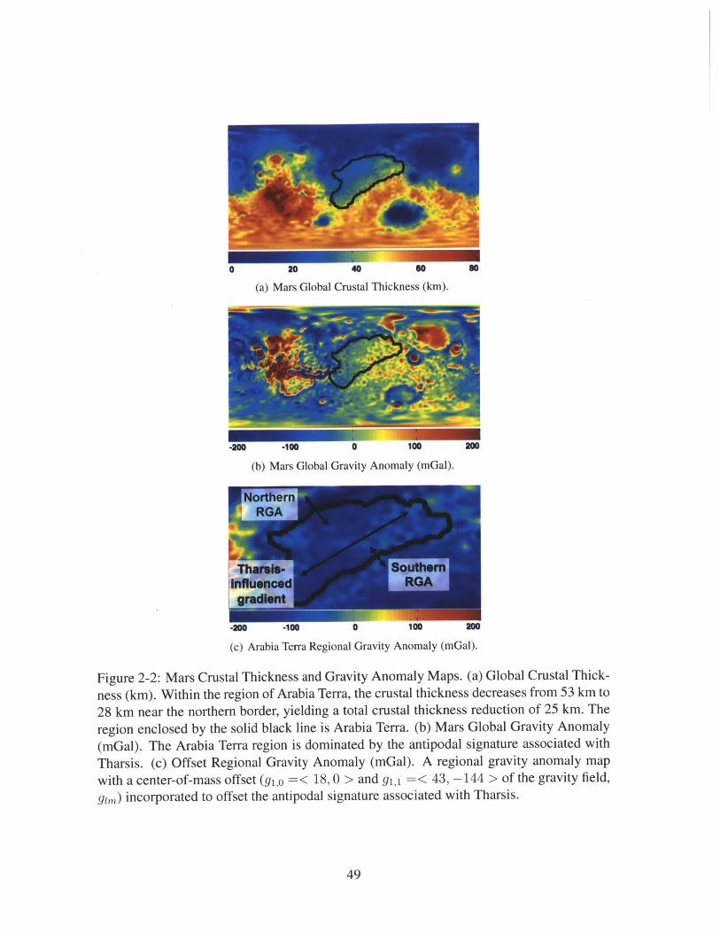
20 40 60

(a) Mars Global Crustal Thickness (km).

-100 U 1UU

(b) Mars Global Gravity Anomaly (mGal).

-200 -100 0 lu ou

(c) Arabia Terra Regional Gravity Anomaly (mGal).

Figure 2-2: Mars Crustal Thickness and Gravity Anomaly Maps. (a) Global Crustal Thick-

ness (km). Within the region of Arabia Terra, the crustal thickness decreases from 53 km to

28 km near the northern border, yielding a total crustal thickness reduction of 25 km. The

region enclosed by the solid black line is Arabia Terra. (b) Mars Global Gravity Anomaly

(mGal). The Arabia Terra region is dominated by the antipodal signature associated with

Tharsis. (c) Offset Regional Gravity Anomaly (mGal). A regional gravity anomaly map

with a center-of-mass offset (gi,o =< 18, 0 > and gi,1 =< 43, -144 > of the gravity field,

gim) incorporated to offset the antipodal signature associated with Tharsis.

49

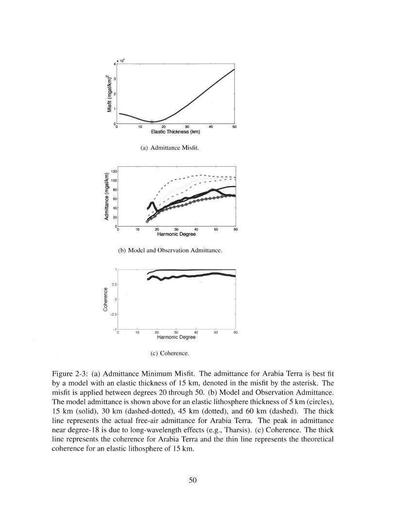
E

E

E

00

-c

3

2

1

x 10

0 10 20 30 40 50

Elastic Thickness (kin)

(a) Admittance Misfit.

20

00

40-

20

000 10 20 30 40 so

Harmonic Degree

(b) Model and Observation Admittance.

1.

.5-

0

.5

10 20 30 40 50 60

Harmonic Degree0

(c) Coherence.

Figure 2-3: (a) Admittance Minimum Misfit. The admittance for Arabia Terra is best fitby a model with an elastic thickness of 15 km, denoted in the misfit by the asterisk. Themisfit is applied between degrees 20 through 50. (b) Model and Observation Admittance.The model admittance is shown above for an elastic lithosphere thickness of 5 km (circles),15 km (solid), 30 km (dashed-dotted), 45 km (dotted), and 60 km (dashed). The thickline represents the actual free-air admittance for Arabia Terra. The peak in admittancenear degree-18 is due to long-wavelength effects (e.g., Tharsis). (c) Coherence. The thickline represents the coherence for Arabia Terra and the thin line represents the theoreticalcoherence for an elastic lithosphere of 15 km.

50

0

0

(a) Highlands' Elevation Load.

Figure 2-4: Conceptual Model. Extending left to right from the southern highlandsto the northern lowlands, respectively, the conceptual model illustrates a crustal cross-section along the Arabia Terra dichotomy boundary. The dark-shaded region representsthe present-day crustal thickness and elevation of Arabia Terra. The dashed lines representthe pre-erosional state of Arabia Terra with a highlands-like elevation and crustal thickness.The light-shaded region represents the eroded amount for each scenario. (a) Highlands' El-evation Load. The erosional load is the spatially-varying elevation difference between themean southern highlands' elevation (pre-erosional Arabia Terra and the present-day ArabiaTerra elevation. (b) Flexural Fit. The erosional load (superimposed on present-day topogra-phy) is designed to match the observed elevation of Arabia Terra by accounting for flexure.Significantly more erosion is required than in the Highlands' Elevation Load.

51

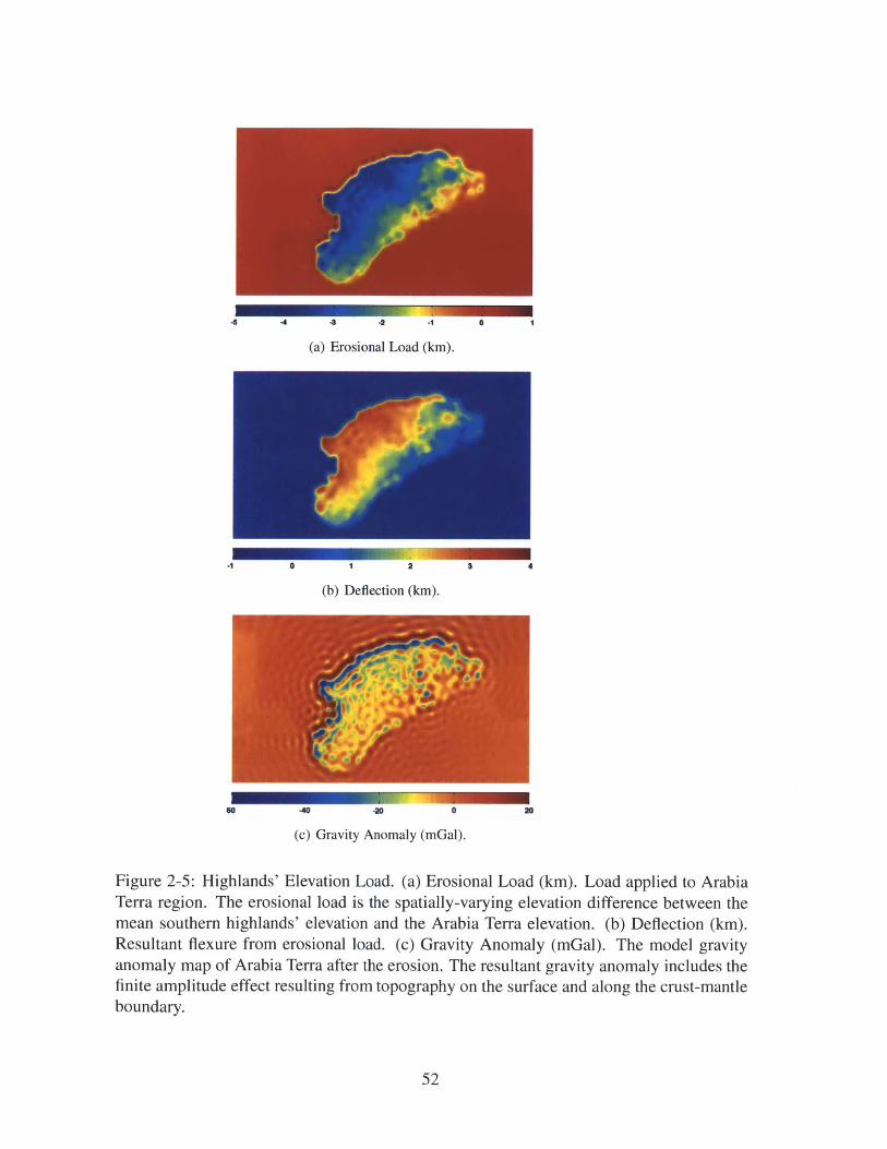
-6 .4 4 -2 .1 0 1

(a) Erosional Load (km).

0 1 2 S 4

(b) Deflection (km).

Go -40 -20 0 20

(c) Gravity Anomaly (mGal).

Figure 2-5: Highlands' Elevation Load. (a) Erosional Load (km). Load applied to ArabiaTerra region. The erosional load is the spatially-varying elevation difference between themean southern highlands' elevation and the Arabia Terra elevation. (b) Deflection (km).Resultant flexure from erosional load. (c) Gravity Anomaly (mGal). The model gravityanomaly map of Arabia Terra after the erosion. The resultant gravity anomaly includes thefinite amplitude effect resulting from topography on the surface and along the crust-mantleboundary.

52

-1

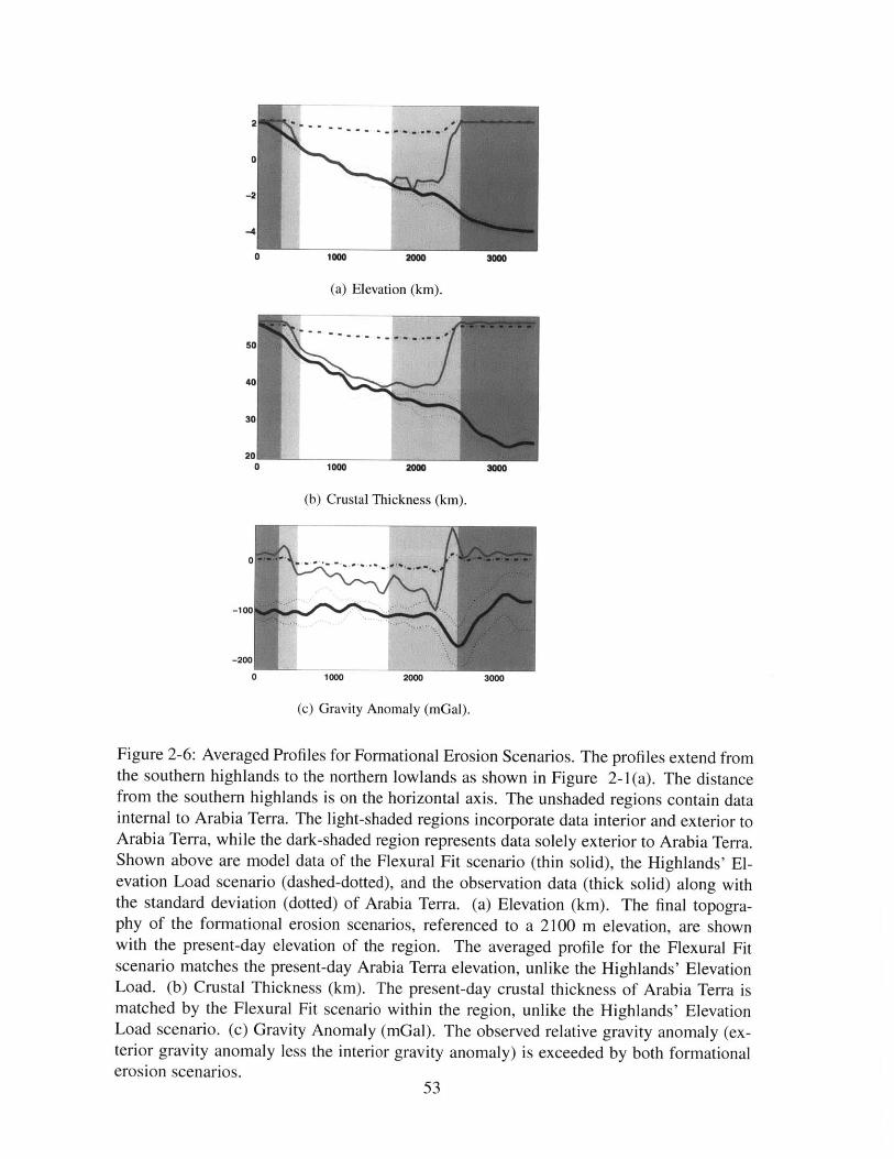
0

0 1000 2000 3000

(a) Elevation (km).

0 1000 2M0 WN0

(b) Crustal Thickness (kn).

-100

0 1000 2000 3000


Figure 2-6: Averaged Profiles for Formational Erosion Scenarios. The profiles extend fromthe southern highlands to the northern lowlands as shown in Figure 2-1(a). The distancefrom the southern highlands is on the horizontal axis. The unshaded regions contain datainternal to Arabia Terra. The light-shaded regions incorporate data interior and exterior toArabia Terra, while the dark-shaded region represents data solely exterior to Arabia Terra.Shown above are model data of the Flexural Fit scenario (thin solid), the Highlands' El-evation Load scenario (dashed-dotted), and the observation data (thick solid) along withthe standard deviation (dotted) of Arabia Terra. (a) Elevation (km). The final topogra-phy of the formational erosion scenarios, referenced to a 2100 m elevation, are shownwith the present-day elevation of the region. The averaged profile for the Flexural Fitscenario matches the present-day Arabia Terra elevation, unlike the Highlands' ElevationLoad. (b) Crustal Thickness (km). The present-day crustal thickness of Arabia Terra ismatched by the Flexural Fit scenario within the region, unlike the Highlands' ElevationLoad scenario. (c) Gravity Anomaly (mGal). The observed relative gravity anomaly (ex-terior gravity anomaly less the interior gravity anomaly) is exceeded by both formationalerosion scenarios.

53

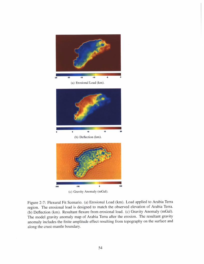
-25 -20 -15 -10 -4 0

(a) Erosional Load (km).

0 5 10 15 20

(b) Deflection (km).

-200 -10 0 100


Figure 2-7: Flexural Fit Scenario. (a) Erosional Load (km). Load applied to Arabia Terra

region. The erosional load is designed to match the observed elevation of Arabia Terra.

(b) Deflection (km). Resultant flexure from erosional load. (c) Gravity Anomaly (mGal).

The model gravity anomaly map of Arabia Terra after the erosion. The resultant gravity

anomaly includes the finite amplitude effect resulting from topography on the surface and

along the crust-mantle boundary.

54

-

1000 2000

(a) Maximum Uniform Erosional Load (km).

1000 2000 -UUU

(b) Maximum Bounded Erosional Load (km).

1- - - -

.. ' a-Si

lg

0 1000 2000 3000


Figure 2-8: Averaged Profiles for Non-Formational Erosion Scenarios. The profiles ex-tend from the southern highlands to the northern lowlands as shown in Figure 2-1(a). Thedistance from the southern highlands is on the horizontal axis. The unshaded regions con-tain data internal to Arabia Terra. The light-shaded regions incorporate data interior andexterior to Arabia Terra, while the dark-shaded region represents data solely exterior toArabia Terra. (a) Maximum Bounded Erosional Load (km). The offset of the present-daytopography from the initial topography (solid line) is shown along with the erosion load(dashed-dotted line) and the deflection (dashed line). (b) Maximum Uniform ErosionalLoad (km). The offset of the present-day topography from the initial topography (solidline) is shown along with the 1300-m uniform erosional load (dashed-dotted line) and thedeflection (dashed line). (c) Gravity Anomaly (mGal). Averaged profile of gravity anomalyfor 450-m erosional load (solid line), maximum uniform erosional load (dashed line), andthe maximum bounded erosional load (dashed-dotted line).

55

U

U

2.9 Tables

56

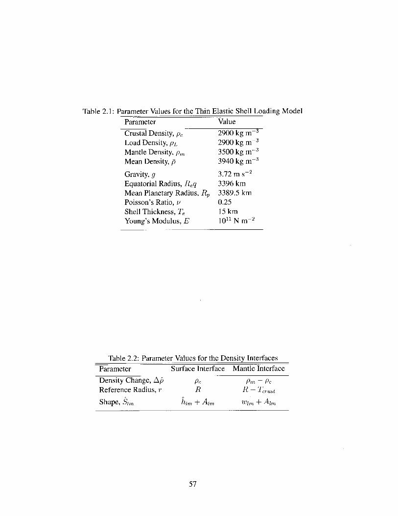
Table 2.1: Parameter Values for the Thin Elastic Shell Loading ModelParameter Value

Crustal Density, Pc 2900 kg m-3Load Density, PL 2900 kg m- 3

Mantle Density, pm 3500 kg m-3Mean Density, p 3940 kg m-3

Gravity, g 3.72 m S-2

Equatorial Radius, Req 3396 kmMean Planetary Radius, Rp 3389.5 kmPoisson's Ratio, v 0.25Shell Thickness, Te 15 kmYoung's Modulus, E 10" N m-2

Table 2.2: Parameter Values for the Density Interfaces

Parameter Surface Interface Mantle Interface

Density Change, A> Pc Pm - PcReference Radius, r R R - Tcrust

Shape, Sim him + Aim Wim + Aim

57

Table 2.3: Erosion Scenario Summary.

Scenario Relative Gravity Anomaly (mGal)a Erosional Load (m)North South North South

Observations 16 ± 4 4 k 2 - -

Highlands' Elevation Load 20 8 5100 0Flexural Fit 80 40 25000 0

Uniform Erosion (450 m) 3 2 450 450

Uniform Erosion: Maximum 7 6 1300 1300Bounded Erosion: Maximum 20 6 5000 300

Uniform Erosion: Best-fit 5 4 750 750Bounded Erosion: Best-fit 16 4 4000 0

aThe uncertainty on the relative gravity anomaly is determined from the standard error on the mean.

58

Chapter 3

A Wet, Heterogenous Lunar Interior:

Lower Mantle & Core Dynamo

Evolution

3.1 Introduction

The Moon is posited to have formed from the coalescence of post-impact debris of a proto-

planet with the young Earth (50; 51). Following the giant impact of the Earth with a

planetary embryo, material scattered beyond the Roche-limit into a proto-lunar disk and

subsequently aggregated to form the Moon (51; 50; 52; 53). The anorthositic and KREEP-

rich (material rich in potassium, rare Earth elements, and phosphorus) composition of the

lunar highlands (54) supports the past existence of a large-scale lunar magma ocean leading

to fractional crystallization and compositional stratification of the Moon(55; 56; 57). Al-

though a 40- to 50-km anorthositic lunar crust is consistent with a magma ocean depth of up

to 1000 km, a lower depth limit may be expected given recent observational data from the

dual Gravity Recovaery and Interior Laboratory (GRAIL) spacecraft (58) that indicates an

average crustal thickness between 34 and 43 km (59). During the final stages of fractional

crystallization from a lunar magma ocean, the last dregs of the melt would be enriched

59

in water and incompatible elements, subsequently crystallizing beneath the anorthositic

crustal lid (60; 61). Further, fractional crystallization would result in a chemically-layered

mantle, which may be supported by some seismic observations (29). Until recently, the

Moon had been thought to have a relatively low volatile content due to a combination of

its low gravity and hot impact origin (62; 63). Accordingly, past studies of the Moon's for-

mation and its chemical and thermal evolution have focused on a bulk Moon with minimal

volatile content and absent of water (64). However, recent geochemical analyses of very-

low-Ti glasses and lunar melt inclusions present compelling evidence that water concentra-

tions of at least 260 ppm and up to 6000 ppm were present in the deep lunar interior prior

to 3 Ga (65; 66). If water was a constituent of the bulk Moon, fractional crystallization of

all but the deep mantle would have resulted in a sequestered source of interior water. Ulti-

mately, in this scenario, a post-magma ocean Moon would contain separate sub-crustal and

deep mantle reservoirs, which may be dually consistent with localized water-rich reservoirs

(>260 ppm) (65), and a bulk magma ocean containing under 100 ppm water (67).

While deuterium to hydrogen (D/H) ratios of measured lunar water in apatite are consistent

with a cometary origin (68), the observed hydrogen fractionation could alternatively result

from water-rich glasses erupted from a source region with terrestrial D/H values, provided

the glasses have undergone kinetic fractionation during post-eruptive degassing (69). (63)

find, absent removal mechanisms that may be responsible for later depletion of terrestrial-

imparted volatiles, a post-formation enhancement of volatiles relative to the silicate Earth

is likely for the Moon.

Regardless of whether the origin of lunar water is indigenous, exogenous or a combination

thereof, water in the deep lunar interior must have been retained from accretion or accreted

prior to and perhaps during lunar magma ocean solidification. Under the lunar magma

ocean model, water would be progressively enriched with incompatible elements during

solidification, and a fraction may have been retained by the lunar mantle (70; 67). Although

it is unclear whether measured water concentrations are representative of the entire lunar

mantle or a water-enriched reservoir (66), the existence and subsequent enrichment of water

in the lunar interior could well have had a significant effect on early lunar thermochemical

60

evolution (64; 71). In particular, water may have aided the cooling of the early Moon (72;

73) in addition to influencing the expression of surface features such as impact basins.

Unlike the Earth (74), deep reservoirs of water within the Moon could conceivably exist

near the core-mantle boundary and, if so, could decrease lower mantle viscosity, possibly

facilitating a prolonged and perhaps vigorous lunar dynamo. While the size and composi-

tion of the lunar core are still a matter of active investigation (75), recent analyses of lunar

samples indicate that the Moon had a dynamo-driven magnetic field from at least 4.2-3.56

Ga, consistent with the presence of an advecting liquid iron-rich core (76; 77; 78; 79).

Given bounds on the lunar core size (80), it may be implausible for homogeneous mantle

convection from secular cooling to generate such a long-lasting dynamo via core convection

(79) without mediation by a thermal blanket (81), impact-induced rotation changes(82),

compositionally stratified mantle convection or, possibly, a water-rich layer near the core-

mantle boundary. Although the cooling history of the Moon is still ambiguous, there is

some evidence, including recovered lunar alkalic igneous rocks, indicative of a late rapid

cooling scenario for the shallow part of the Moon which may have been preceded, or over-

lapped, with a slow cooling phase of the deep Moon (54; 83; 84). Such a scenario would

be consistent with a convective core dynamo. In this study, we address the influence of wa-

ter on lunar evolution by incorporating an attenuating strain rate as a proxy for decreased

viscosity (64; 71; 85) for potential wet regions in the lunar interior. From experimental

studies of the Earth's upper mantle (300 MPa), the presence small amounts of water (~20

wt. ppm) can result in a viscosity reduction by a factor in excess of 100 (71; 85). We ex-

amine the influence of compositional stratification and water via protonic weakening (85)

- proton diffusion into nominally anhydrous minerals - on the deep interior. We utilize

a finite-element thermochemical evolution model and investigate changes in temperature,

modes of heat transport, core-mantle boundary heat flux and surface magnetic field inten-

sity. We then use the core-mantle boundary heat flux to provide constraints on the duration

of core dynamo activity.

61

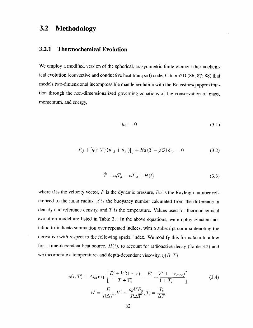
3.2 Methodology

3.2.1 Thermochemical Evolution

We employ a modified version of the spherical, axisymmetric finite-element thermochem-

ical evolution (convective and conductive heat transport) code, Citcom2D (86; 87; 88) that

models two-dimensional incompressible mantle evolution with the Boussinesq approxima-

tion through the non-dimensionalized governing equations of the conservation of mass,

momentum, and energy,

U -,i = 0 (3.1)

-Pj + [71(r, T) (ui,j + upi)]3 + Ra (T - 13C) 6z,r = 0 (3.2)

T + ujTj = rTi + H(t) (3.3)

where U' is the velocity vector, P is the dynamic pressure, Ra is the Rayleigh number ref-

erenced to the lunar radius, 13 is the buoyancy number calculated from the difference in

density and reference density, and T is the temperature. Values used for thermochemical

evolution model are listed in Table 3.1 In the above equations, we employ Einstein no-

tation to indicate summation over repeated indices, with a subscript comma denoting the

derivative with respect to the following spatial index. We modify this formalism to allow

for a time-dependent heat source, H(t), to account for radioactive decay (Table 3.2) and

we incorporate a temperature- and depth-dependent viscosity, Tj(R, T)

S(r, T) =Arexp [E' + V'(1 - r) E'+ V'(1 - rcore)1 (3.4), T + T' 1+TS'

E' - E V, pgVR, , = TRAT' RAT AT

62

where E', V', and T', are the non-dimensionalized activation energy, E, activation volume,

V and surface temperature, Ts, respectively (89; 90), and r1, is the reference viscosity.

The parameter AT represents the temperature difference across the mantle, g is the lunar

surface gravity, and A is a dimensionless pre-exponential factor, herein used to incorporate

viscosity reduction. We apply this viscosity equation in Sections 3.1 and 3.2.

To model the cooling of the core-mantle boundary (CMB), we adjust the model to allow

for a time-varying CMB thermal boundary condition based on

cm kmTiS (3.5)(Pcp V)cr

where T, i is the temperature gradient above the CMB, S is the surface area and V is the

volume of the core, km is mantle conductivity, p is the core density and C, is the core

specific heat. Additionally, we use a particle tracer method (91) to allow for radially-

varying density structures and radioactive element concentrations. In addition to bottom

heating, we include volumetric heating of the mantle, crust, and KREEP layer, starting

from the initial radioactive element concentrations listed in Table 3.2.

Prior lunar mantle convection models (81; 92) have applied a variant of the viscosity equa-

tion,

T(P, T) = AqO exp a E+jv 1 (3.6)1RT

with a partially non-dimensionalized viscosity equation (93) that damps the temperature-

dependence of viscosity (Eq. 3.6). Although the non-dimensionalized Arrhenius equation

(Eq. 3.4) uses radial distance as a proxy for pressure (pgh), ultimately the difference in

gravity between the surface and the core is not a determining factor in the convection model.

The key difference in heat flux predicted by the two viscosity equations is a result of the

damping of the temperature dependence by a scale factor, a. This constant a is partially

offset by the omission of a second exponential term that references viscosity to the CMB as

in Equation 3.4. In Section 3.3.2, we use this variant of the viscosity equation as a proxy for

a set of scenarios in which the pre-overturn temperature of the magma ocean cumulates is

not completely retained, and to illustrate the differences in applying a rheological equation

63

that does not fully account for the temperature dependence of viscosity. We normalize the

viscosity at the CMB to our reference viscosity, 1020 Pa-s.

3.2.2 Water, Pressure, and Rheology

Experimental studies of olivine aggregates and single crystals demonstrate that viscosity

is reduced in the presence of water (protons) (94; 95). (94) found viscosity is reduced by

up to a factor of 140 for saturated olivine, corresponding to 40±20 ppm H, at confining

pressures of 300 MPa. Their re-examination of higher pressure data from (96) further

suggests that the viscosity reduction factor is directly proportional to the concentration of

water in the olivine crystal matrix. Consequently, with the pressure-dependent increase of

water solubility in olivine, we expect a maximum viscosity reduction factor in excess of 140

for a deep lunar mantle (>300 MPa) preferentially enriched in water and approximately a

factor of 140 or less at the near-surface given the lower pressure.

3.2.3 Core Heat Flux & Magnetic Field Intensity

We consider a core dynamo driven by thermal core convection. In this case, a necessary

but not sufficient condition for an internally-generated magnetic field on the Moon is a

heat flux at the core-mantle boundary (CMB) above the critical threshold value, qad, of that

carried conductively along the core adiabat, where

(ad = 4GcPcoreTckcRc (3.7)3cp,core

We define the relevant variables in Table 3.1. Using the energy flux to magnetic field

strength scaling of (97) and assuming constant material properties in the core (see Ta-

ble 3.3), we can employ the following relation as an upper limit for the surface magnetic

field intensity that can be produced from our core heat flux

64

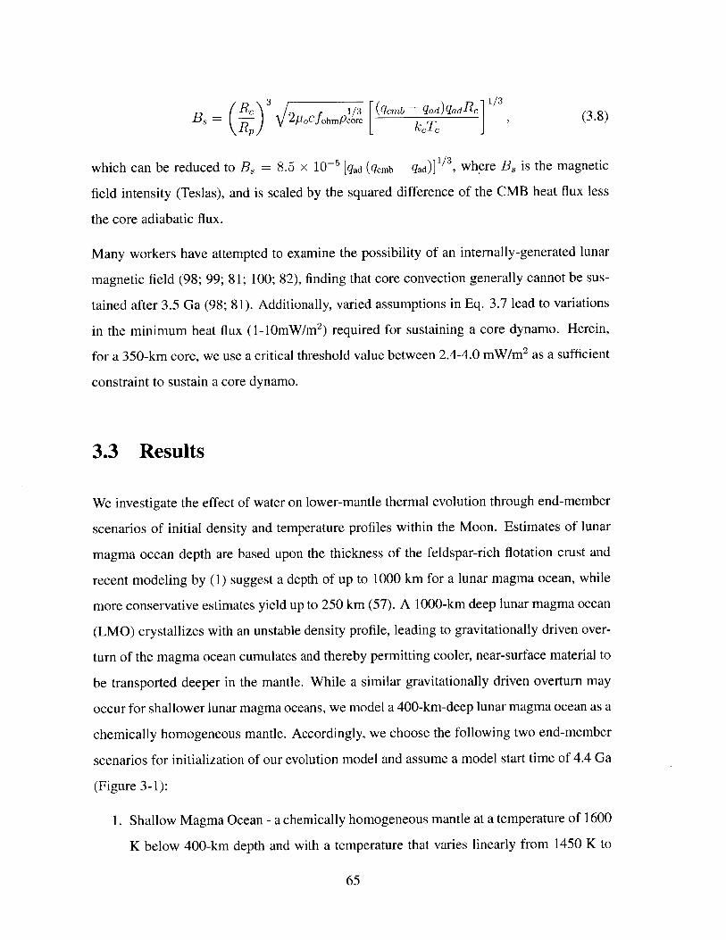
Re f 1,3 [(qcmb - qad)qadRc1BS = \/p 2Cfohmpcore I c 1 1(3.80)

which can be reduced to B, = 8.5 x 10- 5 [qad (qcmb - qad)]/ 3 , where Bs is the magnetic

field intensity (Teslas), and is scaled by the squared difference of the CMB heat flux less

the core adiabatic flux.

Many workers have attempted to examine the possibility of an internally-generated lunar

magnetic field (98; 99; 81; 100; 82), finding that core convection generally cannot be sus-

tained after 3.5 Ga (98; 81). Additionally, varied assumptions in Eq. 3.7 lead to variations

in the minimum heat flux (1-10mW/M2 ) required for sustaining a core dynamo. Herein,

for a 350-km core, we use a critical threshold value between 2.4-4.0 mW/n 2 as a sufficient

constraint to sustain a core dynamo.

3.3 Results

We investigate the effect of water on lower-mantle thermal evolution through end-member

scenarios of initial density and temperature profiles within the Moon. Estimates of lunar

magma ocean depth are based upon the thickness of the feldspar-rich flotation crust and

recent modeling by (1) suggest a depth of up to 1000 km for a lunar magma ocean, while

more conservative estimates yield up to 250 km (57). A 1000-km deep lunar magma ocean

(LMO) crystallizes with an unstable density profile, leading to gravitationally driven over-

turn of the magma ocean cumulates and thereby permitting cooler, near-surface material to

be transported deeper in the mantle. While a similar gravitationally driven overturn may

occur for shallower lunar magma oceans, we model a 400-km-deep lunar magma ocean as a

chemically homogeneous mantle. Accordingly, we choose the following two end-member

scenarios for initialization of our evolution model and assume a model start time of 4.4 Ga

(Figure 3-1):

1. Shallow Magma Ocean - a chemically homogeneous mantle at a temperature of 1600

K below 400-km depth and with a temperature that varies linearly from 1450 K to

65

1600 K from the surface to 400 km depth.

2. Deep Magma Ocean - a chemically-heterogeneous mantle at a post-magma ocean

overturn temperature and density (Figure 3-1). From the surface, the density in-

creases linearly from 3000 to 3500 kg/m3 until 1000-km depth. This model of lunar

convection may be consistent with possible seismic discontinuities of magma ocean

cumulates (29), which may be a result of layering from overturn of the lunar magma

ocean.

Using the fully non-dimensionalized Arrhenius equation (Eq. 3.4), we explore the effect of

water enrichment for a range of CMB temperature boundary conditions. While the lunar

core may be capable of initially retaining a 700-K higher temperature relative to the lower

mantle (98), we examine moderate cases initiated with a temperature difference across the

core-mantle boundary, ATernb < 200 K. In Section 3.3.2, we examine the effect of varying

core radii on our results and employ a temperature-damped viscosity equation (Eq. 3.6) as

a proxy for a deep LMO scenario in which the magma ocean cumulates do not fully retain

their temperature post-overturn.

3.3.1 Shallow Lunar Magma Ocean

For a predominantly chemically homogeneous mantle and no temperature difference across

the CMB, heat flow in the lunar mantle is dominated by conduction. As a result, the core

heat flux is relatively weak and is below the minimum needed to sustain a dynamo for all

of lunar history (Figure 3-2a).

In Figures 3-3d and 3-2d, we observe that a higher CMB temperature difference enhances

the CMB heat flux in the first few hundred million years, and exceeds the minimum CMB

heat flux within the first 0.01 Gyr. We find a core heat flux above the minimum required for

convection cannot be sustained beyond 3.9 Ga, which is too young to produce a dynamo

recorded by lunar samples at 3.56 Ga (79). As expected from Eq. (3.8), the increased CMB

temperature difference results in a greater intensity for the magnetic field at the surface: 2.5

pT and 3.2 pT, for 100 K and 200 K CMB temperature differences, respectively.

66

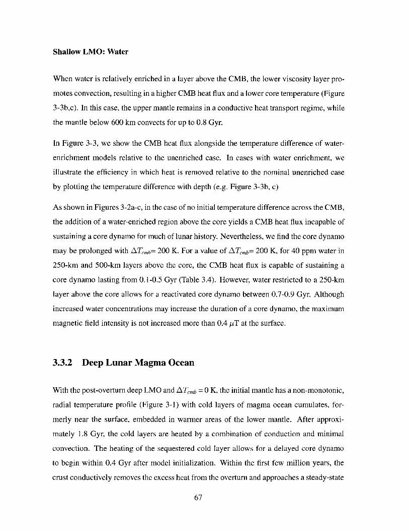
Shallow LMO: Water

When water is relatively enriched in a layer above the CMB, the lower viscosity layer pro-

motes convection, resulting in a higher CMB heat flux and a lower core temperature (Figure

3-3b,c). In this case, the upper mantle remains in a conductive heat transport regime, while

the mantle below 600 km convects for up to 0.8 Gyr.

In Figure 3-3, we show the CMB heat flux alongside the temperature difference of water-

enrichment models relative to the unenriched case. In cases with water enrichment, we

illustrate the efficiency in which heat is removed relative to the nominal unenriched case

by plotting the temperature difference with depth (e.g. Figure 3-3b, c)

As shown in Figures 3-2a-c, in the case of no initial temperature difference across the CMB,

the addition of a water-enriched region above the core yields a CMB heat flux incapable of

sustaining a core dynamo for much of lunar history. Nevertheless, we find the core dynamo

may be prolonged with ATmb= 200 K. For a value of ATemb= 200 K, for 40 ppm water in

250-km and 500-km layers above the core, the CMB heat flux is capable of sustaining a

core dynamo lasting from 0.1-0.5 Gyr (Table 3.4). However, water restricted to a 250-km

layer above the core allows for a reactivated core dynamo between 0.7-0.9 Gyr. Although

increased water concentrations may increase the duration of a core dynamo, the maximum

magnetic field intensity is not increased more than 0.4 pT at the surface.

3.3.2 Deep Lunar Magma Ocean

With the post-overturn deep LMO and A Temb = 0 K, the initial mantle has a non-monotonic,

radial temperature profile (Figure 3-1) with cold layers of magma ocean cumulates, for-

merly near the surface, embedded in warmer areas of the lower mantle. After approxi-

mately 1.8 Gyr, the cold layers are heated by a combination of conduction and minimal

convection. The heating of the sequestered cold layer allows for a delayed core dynamo

to begin within 0.4 Gyr after model initialization. Within the first few million years, the

crust conductively removes the excess heat from the overturn and approaches a steady-state

67

thermal profile.

For these chemically-heterogeneous LMO cases, the upper- and mid- mantle maintain a

conductive heat transport regime, while periodic and sluggish lower mantle convection may

persist for the first 0.6 Gyr (Figure 3-4). As shown in Figure3-5d, this case has a slightly

lower CMB temperature than the shallow LMO scenario with core heat removed via con-

vection at the top of the core. While the layer below the sequestered cold layer convects,

the cold layer is inhibited from participating in convection due to its higher viscosity. Un-

like the shallow LMO scenario, a larger thermal gradient at depth can be maintained due to

the sequestered cold layer. This thermodynamical behavior enables a mantle without water

enrichment to sustain a CMB heat flux within the core dynamo regime for approximately

1.5-2 Gyr (Figure 3-5d).

For increases in ATmb, the initiation of a core dynamo is accelerated by the earlier onset

of lower mantle convection and continues through 2.4 Ga (Table 3.5). Given the more

vigorous convection catalyzed by the higher ATmb, the final core temperature is decreased

as ATemb increases. Furthermore, when ATmb = 200K, a core dynamo is capable of

producing a maximum magnetic field intensity of 3.5 pT at the surface.

In summary, for a deep LMO without a water-enriched lower mantle, we find that the core

heat flux condition for a convective core dynamo can be met until 2.4 Ga.

Deep LMO: Water

By incorporating water within the deep lunar interior through a reduction in viscosity, the

lower lunar mantle more readily sustains a separate convective layer from the remainder

of the lunar mantle (Figure 3-4 g-i). We analyze scenarios containing 20 ± 10 wt. ppm

(factor of 10 viscosity reduction) and 40 ± 20 wt. ppm (factor of 100 viscosity reduction),

within layers of 100 km, 250 km, and 500 km above the CMB. To gauge the effect of water

content in the deep interior, we examine model cases relative to the unenriched wet mantle

case, alongside varying CMB temperature boundary conditions.

Generally, the result of a lower mantle with a relative enrichment in water is a layer of

68

reduced viscosity above the core that convects heat away from the CMB into a sluggishly-

convecting or conducting overlying mantle. A relative enrichment of water enables heat to

be transported out of the core at an increased rate, catalyzed by the sequestered cold-mantle

layer. The effect of water has a potent effect on paleointensities for no CMB temperature

difference, as observed by the 1.3 pT increase in the magnetic field strength for a 250-km-

thick, water-enriched layer (Table 3.5) (although water enrichment generally shortens the

core dynamo timespan due to the more rapid heat loss from the core).

For 40 ppm water in 250-km and 500-km layers above the core, the CMB heat flux gener-

ally allows a core dynamo to be active within 0.01 Gyr of the beginning of the model (Table

3.4) and lasting until 2.9-2.4 Ga, depending on the initial ATmb. These cases all produce

a high heat flux after 3.6 Ga, encompassing the possible high lunar magnetic era of (101).

However, water at the same concentration, restricted to a 100-km layer above the core has

a negligible effect on the heat flux.

Temperature-Damped Convection

We re-examine the deep LMO scenario for 350-km and 450-km core radii, this time using

the temperature-damped viscosity equation (Equation 3.6). For a post-overturn temper-

ature profile, the upper- and mid-mantle remain in the conductive heat transport regime,

with minimal lower mantle convection for the first 0.3 Gyr (Figure 3-1) occurring in the

lower mantle. As for our standard deep LMO scenario, the sequestered cold layer persists

throughout the possible core dynamo era. As a consequence of the temperature dampening,

the sequestered cold layer is able to participate in convection, leading to a major upwelling

and CMB heat flux peak occurring around -0.25 Gyr.

When water is enriched in a layer above the CMB, heat is removed with a greater efficiency,

resulting in a higher CMB heat flux and a lower final core temperature. For 40 ppm water

in 250-km and 500-km layers above the core, the CMB heat flux is capable of sustaining

a core dynamo within the first 0.1 Gyr (Figure 3-7), but may reduce the lifetime of a core

dynamo by 0.5 Ga. In all but one case, increasing the temperature difference across the

69

CMB reduces the end time of the core dynamo era by ~0.2 Gyr while generally producing

higher heat fluxes and hence stronger magnetic fields.

Relative to the nominal deep LMO scenarios presented earlier, the temperature-damped

cases allow for the mantle to transfer more heat earlier in lunar history, constraining the

end time for a possible dynamo era to ~3.3 Ga. Contrary to the undamped case for a deep

LMO with a 350-km core radius, the addition of a water enriched layer can substantially

increase the maximum surface intensity of the magnetic field by up to 40% to 5.1 PT for a

200 K CMB temperature difference.

For an increased core radius of 450 km, the CMB heat flux for an unenriched water case is

negligibly affected (Figure 3-7) while for the 250-km water-enriched layer case CMB heat

flux peak locations and amplitudes vary. The greater variance in heat flux of the water-

enriched case is due to the increase in total water content volume resulting from a larger

core radius. The larger core radius shifts the top and bottom of the water-enriched layer to

a larger radius; so for a constant layer thickness, we have a larger overall volume for the

water-enriched layer. While the heat flux variance is minimal, the 450-km core size results

in stronger surface magnetic fields by a factor of 2-3.5 relative to the 350-km core case.

The increased magnetic field intensities are primarily a result of the increased core radius

(see Eq. 3.8), and demonstrate that the size of the core is a critical factor determining the

maximum field strength observed at the lunar surface. This result derives from the fact

that the surface field intensity scales as the cube of the ratio of core radius to the lunar

radius.

3.4 Discussion

The recent re-analyses of Apollo-era samples for remnant magnetization have likely iden-

tified the existence of an internally-generated field on the Moon between -4.2 and 3.56 Ga

(78). The existence of such a field produced by a lunar core dynamo has been thought to

be untenable for convective core dynamos, with heat fluxes at the CMB unable to sustain a

heat flux in excess of the adiabat beyond 4.0 Ga. Homogeneous models of the lunar mantle,

70

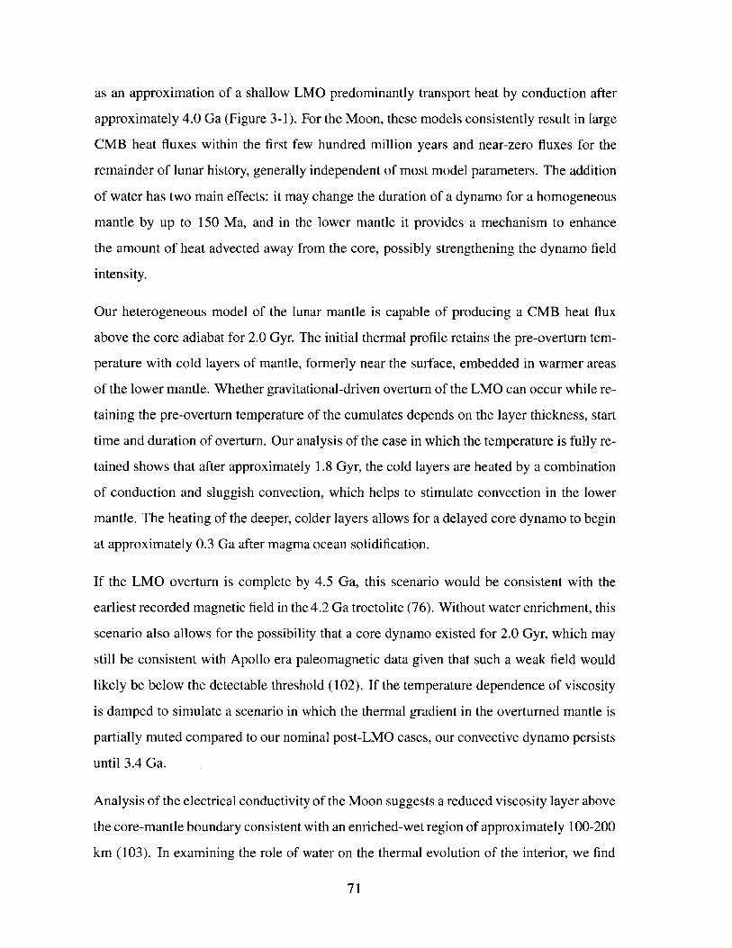
as an approximation of a shallow LMO predominantly transport heat by conduction after

approximately 4.0 Ga (Figure 3-1). For the Moon, these models consistently result in large

CMB heat fluxes within the first few hundred million years and near-zero fluxes for the

remainder of lunar history, generally independent of most model parameters. The addition

of water has two main effects: it may change the duration of a dynamo for a homogeneous

mantle by up to 150 Ma, and in the lower mantle it provides a mechanism to enhance

the amount of heat advected away from the core, possibly strengthening the dynamo field

intensity.

Our heterogeneous model of the lunar mantle is capable of producing a CMB heat flux

above the core adiabat for 2.0 Gyr. The initial thermal profile retains the pre-overturn tem-

perature with cold layers of mantle, formerly near the surface, embedded in warmer areas

of the lower mantle. Whether gravitational-driven overturn of the LMO can occur while re-

taining the pre-overturn temperature of the cumulates depends on the layer thickness, start

time and duration of overturn. Our analysis of the case in which the temperature is fully re-

tained shows that after approximately 1.8 Gyr, the cold layers are heated by a combination

of conduction and sluggish convection, which helps to stimulate convection in the lower

mantle. The heating of the deeper, colder layers allows for a delayed core dynamo to begin

at approximately 0.3 Ga after magma ocean solidification.

If the LMO overturn is complete by 4.5 Ga, this scenario would be consistent with the

earliest recorded magnetic field in the 4.2 Ga troctolite (76). Without water enrichment, this

scenario also allows for the possibility that a core dynamo existed for 2.0 Gyr, which may

still be consistent with Apollo era paleomagnetic data given that such a weak field would

likely be below the detectable threshold (102). If the temperature dependence of viscosity

is damped to simulate a scenario in which the thermal gradient in the overturned mantle is

partially muted compared to our nominal post-LMO cases, our convective dynamo persists

until 3.4 Ga.

Analysis of the electrical conductivity of the Moon suggests a reduced viscosity layer above

the core-mantle boundary consistent with an enriched-wet region of approximately 100-200

km (103). In examining the role of water on the thermal evolution of the interior, we find

71

that water enrichment at depth is likely to further decrease the temperature of the lower

mantle over time and, depending on the water concentration and regional extent, this may

shorten or lengthen the duration of a possible core dynamo by as much as 600 Ma. With a

range of density and temperature profiles, the addition of water in the deep interior, we find

that water acts as a catalyst for transporting heat out of the deep mantle. By incorporating

the temperature dependence of viscosity, this effect is more pronounced and generates a

heat flux in most cases exceeding 4 mW/m2.

We find that water-enriched regions provide a stronger CMB heat flux. Using Eq. 3.8, an

upper limit for the magnetic field intensity can be produced from our core heat flux. For

a deep LMO case with 40±20 ppm water at 500 km above a 350-km core, the heat flux

could promote a 5-pT magnetic field at the surface, compared with up to 3.5 pT in cases

without water enrichment. Further, we find varying the core radius (see Eq. 3.8) results

in a minimal change to the core heat flux, but causes substantial changes in the surface

magnetic field strength.

With the exception of a KREEP layer at the near surface, our temperatures do not exceed

the bulk solidus and thus melt quantities are neglected. For larger quantities of melt, the par-

titioning of water and the amount of melt will play dominant roles in determining whether

a viscosity reduction or increase is likely for melt under hydrous conditions (94). The

very-low-Ti glasses recently discovered to contain water are theorized to originate from a

heterogeneous mantle source, including a KREEP component, at less than 520-km depth

(65; 64; 104; 105). If only a small amount of KREEP was retained near the surface, the

remainder along with its radioactive element and water content may have foundered with

a dense layer of cumulates below. Given our results, it is likely that under these circum-

stances, water could have played an influential role in promoting a higher CMB heat flux

and could have promoted core dynamo activity beyond 3.7 Ga.

Although our shallow LMO cases are unable to sustain the minimum CMB heat flux beyond

3.7 Ga, we note that a growing solid inner core is likely to reduce the minimum CMB

heat flux necessary to main a superadiabatic liquid outer core (106; 100), thus potentially

allowing a chemically homogeneous mantle to sustain a core dynamo. In general, these

72

shallow LMO cases illustrate that water enrichment above the CMB promotes a stronger,

higher CMB heat flux, extending a lunar core dynamo period by up to 150 Ma.

3.5 Summary

A homogeneous, dry model of the lunar mantle is biased to predominantly conduction

after approximately 4.0 Ga, after which time it is generally unable to support a convective

core dynamo without external mediation of a thermal blanket (81), impact-induced rotation

changes (82), or, as we show in this study, the addition of mantle water. For the Moon,

these models tend to result in large CMB heat fluxes within the first few hundred million

years, and very low fluxes for the rest of lunar history, consistent with prior models (98;

81). We find that a deep lunar magma ocean after gravitationally driven overturn may

sustain a core dynamo on timescales longer than the latest paleomagnetic data (78; 79),

through 2.4 Ga. Based on the core dynamo scaling model of (97) for a 350-km core radius,

our results yield a maximum magnetic field intensity of 3.5 pT without water enrichment

and 5.1 pT with water enrichment. Additionally, we find that the observed maximum

magnetic field strength at the surface is strongly dependent on the lunar core radius. For

the homogeneous and heterogeneous mantle cases, enriched water in the lower mantle

acts as a catalyst for transporting heat out of the deep mantle due to the reduced viscosity

from protonic weakening (85). If water was transported or retained preferentially in the

deep interior, even in small amounts (<20 ppm), it would have played a significant role

in transporting heat out of the deep interior and reducing the lower mantle temperature.

Water enriched in the lower mantle could have influenced the timing by up to 1.0 Gyr and

enhanced the vigor of a lunar core dynamo.


I thank Linda Elkins-Tanton for temperature and density data provided for a post-overturn

lunar magma ocean, Shijie Zhong for assistance in the Citcom2D thermal evolution model,

73

and Benjamin Weiss for assistance and comments. This work was supported by the NASA

Lunar Science Institute and a NASA Lunar Advanced Science and Exploration Research

grant to BPW.

3.7 Figures

74

1500

1000

500300 1000 1700

Temperature (K)

Figure 3-1: Initial temperature and density profiles used in our convective models withATmb = 200 K. Shown is the temperature profile of the deep LMO scenario (blue solidline) as determined by (1) compared to the shallow LMO (red dashed line).

75

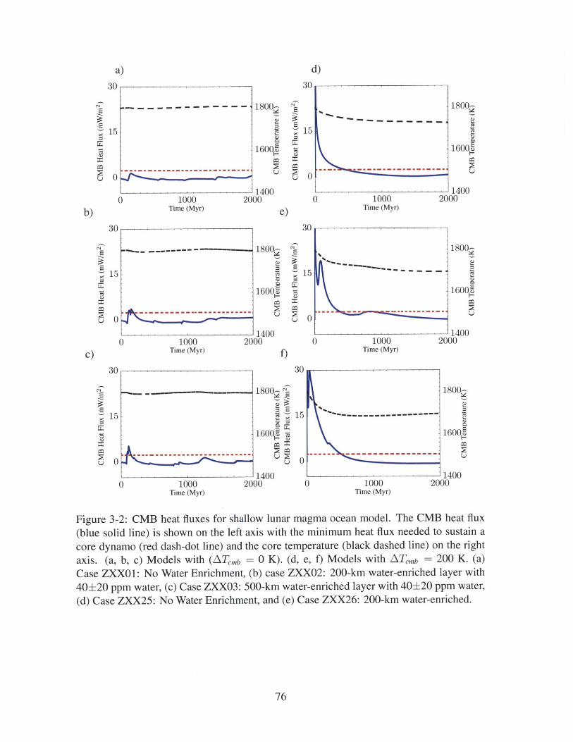
30 30

S1800- 1800-

15 15

1600 = 1600E

0 0

1400 14000 1000 2000 0 1000 2000

b) Time (Myr) e) Time (Myr)

30 30

2 - 18002 180022%

15 15

1600 -1600E

0 0

1400 14000 1000 2000 0 1000 2000

C) Time (Myr) 0 Time (Myr)

30 30

-1800-2 1800-

15 15 ----------------

1600E 1600E

U0-----------------------

1400 14000 1000 2000 0 1000 2000

Time (Myr) Time (Myr)

Figure 3-2: CMB heat fluxes for shallow lunar magma ocean model. The CMB heat flux(blue solid line) is shown on the left axis with the minimum heat flux needed to sustain acore dynamo (red dash-dot line) and the core temperature (black dashed line) on the rightaxis. (a, b, c) Models with (ATmb = 0 K). (d, e, f) Models with ATmb = 200 K. (a)

Case ZXX0I: No Water Enrichment, (b) case ZXX02: 200-km water-enriched layer with40±20 ppm water, (c) Case ZXX03: 500-km water-enriched layer with 40±20 ppm water,(d) Case ZXX25: No Water Enrichment, and (e) Case ZXX26: 200-km water-enriched.

76

a) d)

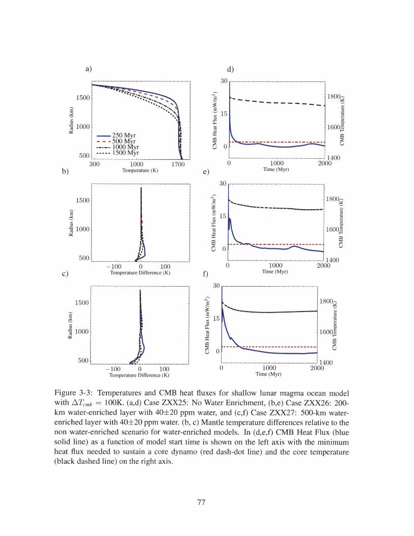
a)

1500

1000

5001

d)

300 1000 1700b) Temperature (K)

1500-

E

1000

1;500

-100 0 100C) Temperature Difference (K)

1500

1000

500-100 0 100

Temperature Difference (K)

30

C)

15

0

0e)

30

2U

U

15

0

0

f)30

15

U 0

0

1000Time (Myr)

1000Time (Myr)

1000Time (Myr)

18002

C

1600-

- 14002000

18002

CL1600~

- 14002000

18002

1600E

-114002000

Figure 3-3: Temperatures and CMB heat fluxes for shallow lunar magma ocean modelwith ATcmb = lOOK. (a,d) Case ZXX25: No Water Enrichment, (b,e) Case ZXX26: 200-km water-enriched layer with 40±20 ppm water, and (c,f) Case ZXX27: 500-km water-enriched layer with 40+20 ppm water. (b, c) Mantle temperature differences relative to thenon water-enriched scenario for water-enriched models. In (d,e,f) CMB Heat Flux (bluesolid line) as a function of model start time is shown on the left axis with the minimumheat flux needed to sustain a core dynamo (red dash-dot line) and the core temperature(black dashed line) on the right axis.

77

---250 Myr0500 Myr

-1000 Myr...... 1500 Myr I

.

---- -----------------------

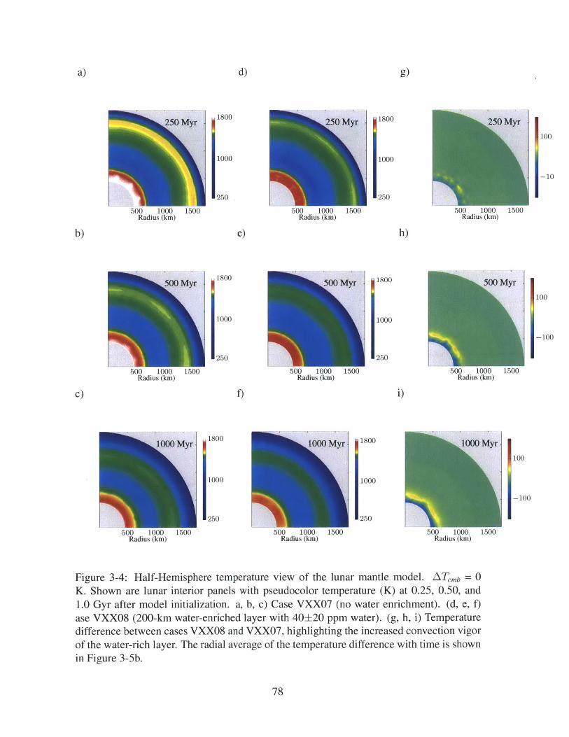
a) d) g)

250 Myr 1800 250 Myr 1800 250 Myr

100

1000 1000

-10

250 250

500 1000 1500 500 1000 1500 500 1000 1500Radius (ki) Radius (km) Radius (km)

b) e) h)

500 Myr 1800 500 Myr 1800 500 Myr

100

1000 1000

-100

250 1250

500 1000 1500 500 1000 1500 500 1000 1500Radius (km) Radius (km) Radius (km)

c) f) i)

l000Myr 1800 Myr 1800 lOMyT100

1000 1000

-100

250 250

500 1000 1500 500 1000 1500 500 1000 1500Radius (km) Radius (km) Radius (km)

Figure 3-4: Half-Hemisphere temperature view of the lunar mantle model. ATmb = 0K. Shown are lunar interior panels with pseudocolor temperature (K) at 0.25, 0.50, and1.0 Gyr after model initialization. a, b, c) Case VXX07 (no water enrichment). (d, e, f)ase VXX08 (200-km water-enriched layer with 40±20 ppm water). (g, h, i) Temperaturedifference between cases VXX08 and VXX07, highlighting the increased convection vigorof the water-rich layer. The radial average of the temperature difference with time is shownin Figure 3-5b.

78

a)

b)

*0C,

1500

1000

500300

1500

1000

500

C)

1500

1000

500

1000Temperature (K)

1700

-100 0 100Temperature Difference (K)


d)30 -

N15

0

0e)

30

X 15

Q0

0

U

30

15

0

0

1000Time (Myr)

1000Time (Myr)

1000Time (Myr)

18002

1600

- 14002000

18002

1600=

U

- 14002000

18002

1600E

- 14002000

Figure 3-5: Temperatures and heat fluxes for deep lunar magma ocean model with ATcmb =0 K. (a,d) Case VXX07: No Water Enrichment, (b,e) Case VXX08: 200-km water-enrichedlayer with 40±20 ppm water, (c,f) Case VXX09: 500-km water-enriched layer with 40±20ppm water, The radially-averaged temperature in time is shown for Case ZXXOI in panel(a) with panels (b,c) tracking the temperature differences with time relative to Case VXX07.In (d, e, f), the CMB heat flux (blue solid line) is shown on the left axis with the minimumheat flux needed to sustain a core dynamo (red dash-dot line) and the core temperature(black dashed line) on the right axis.

79

- %

- 250 Myr- - -500 Myr-- 1000 Myr----. 1500 Myr

- ~. ~ ~.

~4. ~. .. ~

.4. .. . .. .

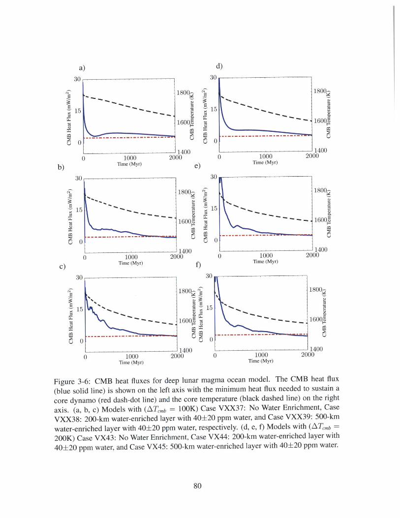
a) d)

30 30

1800- 1800,

15 15

1600E 1600E

U 0 U 0

1400 14000 1000 2000 0 1000 2000

b) Time (Myr) e) Time (Myr)

30 30

1800 1800--

15 15

1600 1600E

U 0 0

1400 14000 1000 2000 0 1000 2000

C) Time (Myr) Time (Myr)

30 30

18002 m18002

15 15

1600 1600E

U 0 0

1400 14000 1000 2000 0 1000 2000

Time (Myr) Time (Myr)

Figure 3-6: CMB heat fluxes for deep lunar magma ocean model. The CMB heat flux

(blue solid line) is shown on the left axis with the minimum heat flux needed to sustain a

core dynamo (red dash-dot line) and the core temperature (black dashed line) on the right

axis. (a, b, c) Models with (ATmb = lOOK) Case VXX37: No Water Enrichment, Case

VXX38: 200-km water-enriched layer with 40±20 ppm water, and Case VXX39: 500-km

water-enriched layer with 40±20 ppm water, respectively. (d, e, f) Models with (ATmb =

200K) Case VX43: No Water Enrichment, Case VX44: 200-km water-enriched layer with

40±20 ppm water, and Case VX45: 500-km water-enriched layer with 40±20 ppm water.

80

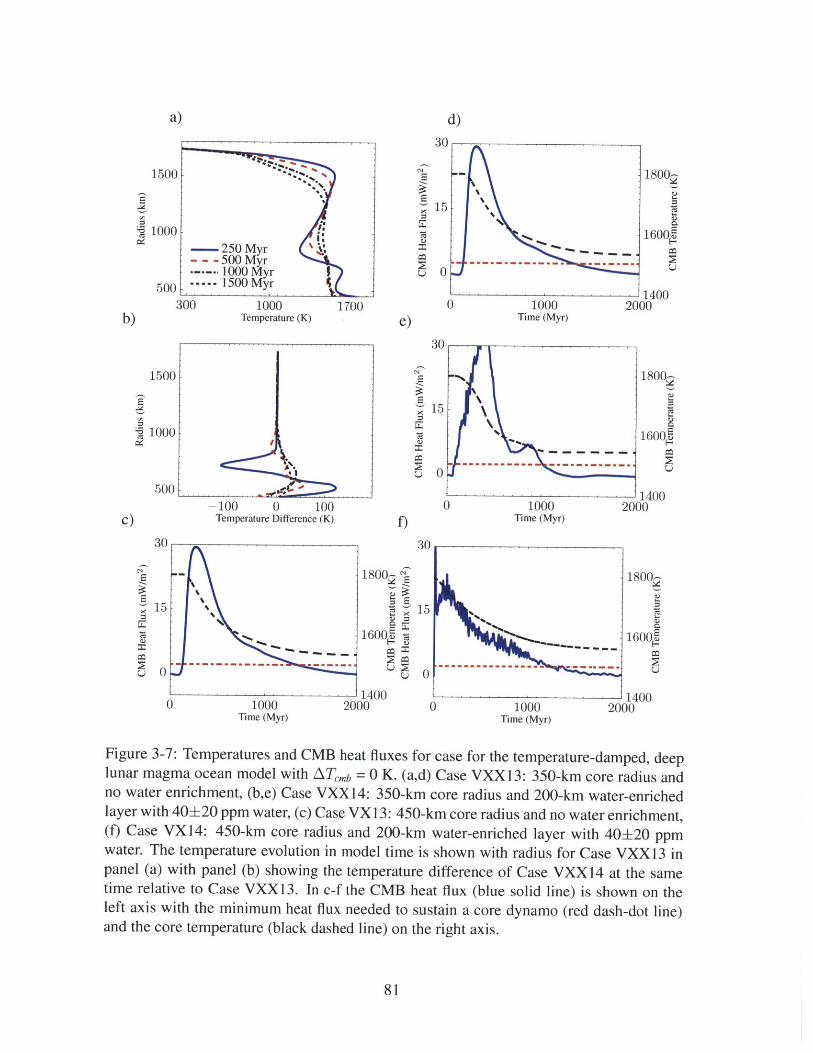
d)30

1000Temperature (K)


1000Time (Myr)

Figure 3-7: Temperatures and CMB heat fluxes for case for the temperature-damped, deeplunar magma ocean model with ATemb = 0 K. (a,d) Case VXX 13: 350-km core radius andno water enrichment, (b,e) Case VXX14: 350-km core radius and 200-km water-enrichedlayer with 40±20 ppm water, (c) Case VX13: 450-km core radius and no water enrichment,(f) Case VX14: 450-km core radius and 200-km water-enriched layer with 40±20 ppmwater. The temperature evolution in model time is shown with radius for Case VXX13 inpanel (a) with panel (b) showing the temperature difference of Case VXX14 at the sametime relative to Case VXX 13. In c-f the CMB heat flux (blue solid line) is shown on theleft axis with the minimum heat flux needed to sustain a core dynamo (red dash-dot line)and the core temperature (black dashed line) on the right axis.

81

4. 4%

- 250 Myr- - -500 Myr----. 100 Myr

----- 1500 Myr

2q15

I fi

b)

E

00 1700

1800-

1600E

1

400

1500

1000

5003

1500

1000

500

C)30

0

0e)

30

12000

2

15

0

\.

1800-

16002

0f)

2q

1000Time (Myr)

1000Time (Myr)

1000Time (Myr)

30

15

0

.4

.4.4

.44%

5%~ _ - - -

18002 N

16000

U

15

0

0

14002000

18002

1600E

114002000

-- 14002000 0

a)

I

------.---.--

3.8 Tables

82

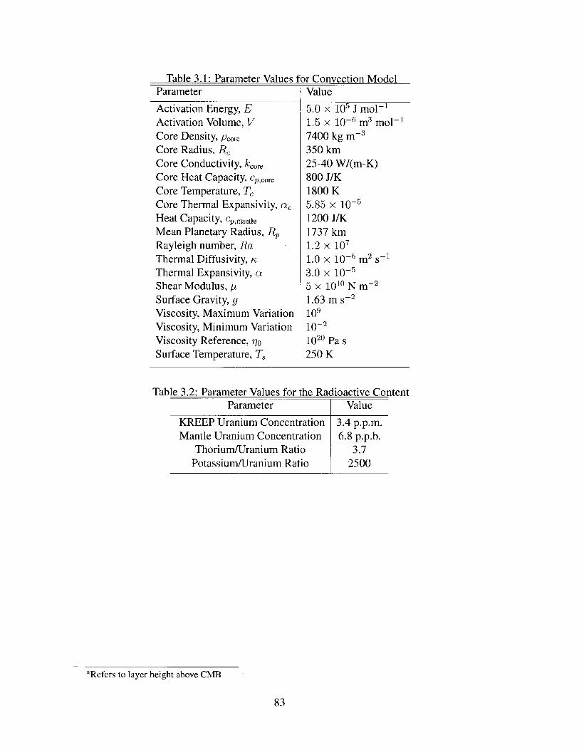
Table 3.1: Parameter Values for Convection ModelParameter

Activation Energy, EActivation Volume, VCore Density, PcoreCore Radius, R,Core Conductivity, kcoreCore Heat Capacity, Cp,core

Core Temperature, T,Core Thermal Expansivity, a,Heat Capacity, Cp,mantle

Mean Planetary Radius, RpRayleigh number, RaThermal Diffusivity, r,Thermal Expansivity, aShear Modulus, pSurface Gravity, gViscosity, Maximum VariationViscosity, Minimum VariationViscosity Reference, rmoSurface Temperature, T,

Value

5.0 x 10' J mol'1.5 x 10-6 m3 mol-17400 kg M-3

350 km25-40 W/(m-K)800 J/K1800 K5.85 x 10-51200 J/K1737 km1.2 x 107

1.0 x 10-6 m 2 S13.0 x 10-55 x 1010 N m-21.63 m S-210910-21020 Pa s250 K

Table 3.2: Parameter Values for the Radioactive ContentParameter Value

KREEP Uranium Concentration 3.4 p.p.m.Mantle Uranium Concentration 6.8 p.p.b.

Thorium/Uranium Ratio 3.7Potassium/Uranium Ratio 2500

83

aRefers to layer height above CMB

Table 3.3: Parameter Values for Magnetic Field IntensityParameter Value

Ratio of ohmic to total dissipation, fohm IConstant of proportionality, c 0.63

Magnetic permeability of free space, [to 1.26 x 10-6

Table 3.4: Shallow Lunar Magma Ocean: CMB Heat Fluxes.

Scenario Input Parameters Dynamo Regime Maximum SurfaceCMB AT (K) Water Layera(km) AH Begin (My) End (My) Field Intensity (tT)

ZXX01 0 0 1 - - -ZXX02 0 250 10-2 100 190 1.3ZXX03 0 500 10-2 90 150 1.6ZXX04 0 100 10-2 - -

ZXX05 0 500 10-1 100 150 1.2ZXX06 0 100 10-1 - - -

ZXX25 100 0 1 0 180 2.5ZXX26 100 250 10-2 0 470 2.6ZXX27 100 500 10-2 0 390 2.9ZXX28 100 100 10-2 0 180 2.5ZXX29 100 500 10-1 0 390 2.5ZXX30 100 100 101 0 180 2.5

ZXX3I 200 0 10-2 0 460 3.2ZXX32 200 250 10-2 0 410** 3.2ZXX33 200 500 10-2 0 520 3.5ZXX34 200 100 10-2 0 460 3.2ZXX35 200 500 10-1 0 690 3.2ZXX36 200 100 10-1 0 460 3.2

84

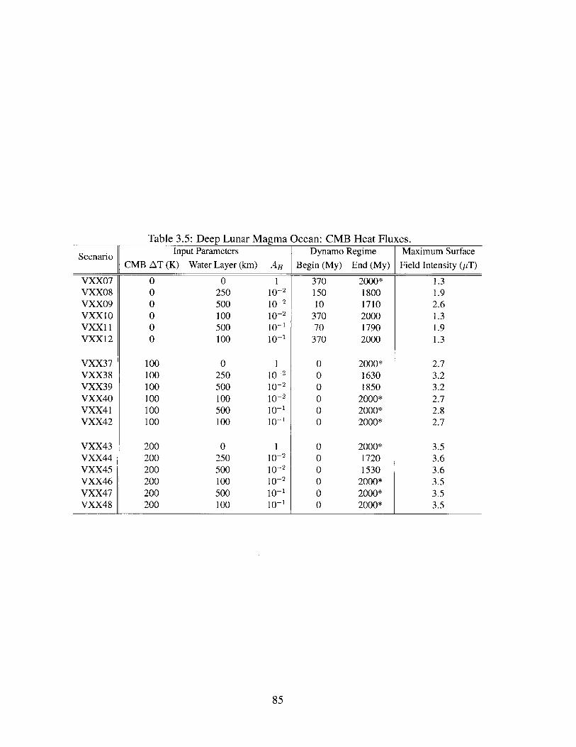
Table 3.5: Deep Lunar Magma Ocean: CMB Heat Fluxes.

Scenario Input Parameters Dynamo Regime Maximum SurfaceCMB AT (K) Water Layer (km) AH Begin (My) End (My) Field Intensity (pT)

VXX07 0 0 1 370 2000* 1.3VXX08 0 250 10-2 150 1800 1.9VXX09 0 500 10-2 10 1710 2.6VXXIO 0 100 10-2 370 2000 1.3VXX1 0 500 10-1 70 1790 1.9VXX12 0 100 10-1 370 2000 1.3

VXX37 100 0 1 0 2000* 2.7VXX38 100 250 10-2 0 1630 3.2VXX39 100 500 10-2 0 1850 3.2VXX40 100 100 10-2 0 2000* 2.7VXX41 100 500 10-1 0 2000* 2.8VXX42 100 100 10-1 0 2000* 2.7

VXX43 200 0 1 0 2000* 3.5VXX44 200 250 10-2 0 1720 3.6VXX45 200 500 10-2 0 1530 3.6VXX46 200 100 10-2 0 2000* 3.5VXX47 200 500 10-1 0 2000* 3.5VXX48 200 100 10-1 0 2000* 3.5

85

Table 3.6: Temperature-Damped Viscosity: CMB Heat Fluxes.

Scenario Input Parameters Dynamo Regime Maximum Surface

Core Radius (km) CMB AT (K) Water Layer (km) AH Begin (My) End (My) Field Intensity (pT)

VXX13 350 0 0 1 130 1330 3.4VXX14 350 0 250 10-2 80 1020 4.0VXX15 350 0 500 10-2 0 870 4.2VXX16 350 0 100 10-2 130 1330 3.4VXX17 350 0 500 10-1 20 1080 3.9VXX18 350 0 100 101 130 1330 3.4

VXX49 350 200 0 1 0 1220 3.5VXX50 350 200 250 10-2 0 800 4.4VXX51 350 200 500 10-2 0 810 5.1VXX52 350 200 100 10-2 0 1220 3.5VXX53 350 200 500 10-1 0 780 4.5VXX54 350 200 100 10-1 0 1220 3.5

VX13 450 0 0 1 130 1240 8.4VX14 450 0 250 10-2 0 1170 8.4VX15 450 0 500 10-2 0 680 15.0VX16 450 0 100 10-2 70 920 10.1VX17 450 0 500 10~1 20 840 11.4VX18 450 0 100 10-1 90 1150 8.3

VX49 450 200 0 1 0 1120 8.8VX50 450 200 250 10-2 0 1000 11.6VX51 450 200 500 10-2 0 650 15.3VX52 450 200 100 10-2 0 1010 10.9VX53 450 200 500 10-1 0 820 12.5VX54 450 200 100 10-1 0 1020 9.2

a* The dynamo regime is still active at this time.a** The CMB heat flux enters the dynamo regime for approximately 0.1 Gyr near 0.8 Gyr after model

initialization.

86

Chapter 4

A Wet Lunar Mantle: Basin

Modification

4.1 Introduction

As mentioned in the previous chapter, during the final stages of fractional crystallization

from a lunar magma ocean, the last dregs of the melt would be enriched in water and

incompatible elements, subsequently crystallizing beneath the anorthositic crustal lid (60;

61). Thus, a post-magma ocean Moon would contain a sub-crustal water-rich reservoir

(>260 ppm) (65) and may have influenced the expression of surface features such as impact

basins.

Similarly-sized lunar basins exhibit a predictable trend in the depth-to-diameter ratios, with

older basins revealing shallower topographic profiles than their younger counterparts (107).

Given the predicted high temperatures for the early Moon (108; 1), it is expected viscoelas-

tic relaxation more pervasively influenced the evolution of the impact basin topography in

early lunar history, such as Transquilitatis and South Pole-Aitken basins (109), and may

have been enhanced by near-surface water reservoirs.

In this study, we address the influence of water on lunar evolution by incorporating an

attenuating strain rate (i.e. decreased viscosity) (64; 71; 85) for potential wet regions in

87

the lunar interior. From experimental studies of the Earth's upper mantle (300 MPa), the

presence small amounts of water ( 20 wt ppm) can result in a viscosity reduction by a

factor in excess of 100 Pa-s (71; 85). For the near-surface effect of water, we construct

profiles for pre-relaxed lunar basins [Sori & Zuber in prep.] and examine the influence

of impact heating, dislocation creep, and water on basin evolution through a viscoelastic

model of basin loading to provide insight into the lunar thermal history and the existence

of near-surface water reservoirs.

4.2 Methodology

4.2.1 Impact Heating & Initial Basin State

A projectile impacting a planetary surface initially forms a transient crater of diameter, Dat

which can be related to the final rim diameter, D, by

D = 1.32D. 086D 0.086 (4.1)

where Dsc represents the single-to-complex transition diameter (110), approximately 20

km, as determined by (111). The transient crater diameter from Equation 4.1 is used to

determine the impactor diameter in

Dp = 1.34g- 2 2 v0.44 (4.2)

derived from (112). For our calculations, we assume a vertical impactor velocity, vi, of 15

km/s (113).

We can determine the temperature increase from waste heat generated by decompression

from a shock state as derived by (114),

88

P6 C2 (f -In f - 1) (4.3)A TS(N 6 2poSCp S2

)-12P 6S ( 4F6 S(4)f(P) C 2po C 2Po

where P6 is the peak shock pressure, Ps, less the initial static pressure, PO. Since our

estimates of impact heating are near the surface, we assume P6=P. Table 4.1 contains the

values for constants employed in the above equations.

Within the isobaric core at depth d, = R(1Oa2)v 2 and radius, r, = R(101)v 1, the peak

shock pressure is equal to Pc, and decays inversely with distance according to the formula

(115; 112).

rc1.84+2.61 log oiPs Pe- (4.5)

where P, is defined by

Pc = poae (C + Sue) . (4.6)

Per (114), we assume the target and impactor have the same density and the particle velocity

of the isobaric core, u, = 0.5vi. Using improved estimates of depth-to-diameter ratios

for impacts basins, we construct profiles for pre-relaxed lunar basins from a power-law

extrapolation of 60-200 km basins [Sori & Zuber in prep.]. For simplicity, we assume an

initial parabolic depth profile with the maximum depth at the basin center.

4.2.2 Viscoelastic Relaxation

We employ a viscoelastic model (CitcomVE) based on a Citcom2D framework (116; 86;

87; 88) that models incompressible viscoelastic and maxwellian mantle dynamics. We

89

use the following governing equations of the conservation of mass and momentum, and

gravitational perturbation (117) in addition to the rheological equation,

Uii = 0, (4.7)

ai ,j + Poj - pigj - polgluij 6 i, = 0, (4.8)

#,i = -47rGpl, and (4.9)

-i7 + T-&j = - (P + P ) 6 + r(r, T) (ui,j + uj,). (4.10)

where P is the dynamic pressure, Ra is the Rayleigh number referenced to the lunar radius,

T is the temperature, and n, is normal vector in the radial direction. We use the temperature

and viscosity from our convection model in Chapter 3. The above equations use Einstein

notation to indicate summation over repeated indices, with a subscript comma denoting the

derivative with respect to the following spatial index.

4.3 Observations & Constraints

The cooling history of the moon is still ambiguous, though there is some evidence, includ-

ing recovered lunar alkalic igneous rocks, which suggest a late rapid cooling scenario for

the shallow part of the moon, which may have been preceded, or overlapped, with a slow

cooling phase of the deep moon (54; 83; 84). The impact basins, which dominate the lunar

terrain through the Late Imbrian (107), can provide constraints on the thermal history, but

require an understanding of the role of impact heating, rheology, local radioactive heating

and water concentration, and subsequent modification mechanisms (e.g. (118; 119)).

90

4.4 Shallow Upper Mantle Water & Basin Relaxation

The existence of a water-enriched near-surface layer is predicted by the lunar magma ocean

model (67). Water, would be enriched, with the incompatible elements forming a wet,

radiogenically-enhanced layer (urKREEP) beneath the lunar crust (70; 61). It has been

hypothesized that the layer, all or in part, may have foundered and or mixed with the other

cumulates during the suspected overturn of the lunar magma ocean (120; 81). The existence

of the PKT (Procellarum KREEP Terrane) on the lunar surface suggests that a urKREEP

layer, possibly mixed with other cumulates, existed near the surface post-overturn (70).

Herein, we investigate the influence of viscoelastic relaxation of basins, incorporating the

effects of impact heating, KREEP, and water and using the Mendel-Rydberg basin for our

scenarios.

The very-low-Ti glasses discovered to contain water are theorized to come from a het-

erogeneous mantle source, including a urKREEP component, at less than 520-km depth

(65; 64; 104; 105). This suggests that there still exists some of the original urKREEP layer

in the upper mantle. Our results on basin relaxation indicate a near-surface source of water-

enriched, urKREEP, would have a substantial effect on the final topographic profile of a

lunar basin. Unless only a small amount of urKREEP remains near the surface, the radio-

genic content and water concentration would need to be determined in order to deduce any

relevant information on the thermal state from the geomorphic properties of lunar basins.

As determined by our results, the influence of water at the near-surface aids in viscoelastic

basin relaxation and has an increasing effect with increasing radiogenic content.

4.5 Results & Discussion

We use representative lunar density and temperature profiles and evolve temperature based

on Chapter 3 from the time of impact until the present. The water content is represented as

a region of reduced viscosity, and radioactive heat generation is included via a thin 20-km

KREEP layer containing radioactive element concentrations. Our temperature- and depth-

91

dependent rheology is referenced to a viscosity of 102 Pa-s with a maximum viscosity

variation of 10' Pa-s. With the pre-relaxed basin diameter, we estimate the impact heating

based on the shock-increased pressure as derived in our methodology. As our baseline,

we use a dry mantle with uniform material properties and no KREEP. Within the first few

million years, the crust conductively cools the excess heat from the overturn and approaches

a steady-state thermal profile. We compare basins formed at 0.1, 0.3, 0.7 and 1.0 Gyr.

4.5.1 Near-Surface KREEP Layer

The inclusion of a sub-crustal layer of KREEP on the Moon may have important impli-

cations for the viscoelastic relaxation of basins. We apply temperature profiles from our

convection model (Chapter 3) with varying KREEP content to determine the effect on basin

relaxation. Figure 4-1 shows the present-day basin depth as a function of basin formation

age. We find that for a near-surface concentration of KREEP, basin relaxation is enhanced

by 10% at 100 Myr and up to 30% at 1 Gyr.

4.5.2 KREEP Component & Water

The existence of a sub-crustal KREEP layer is predicted by the lunar magma ocean model

and is expected to be commensurate with an enriched zone of water. We examine the effect

of water on the relaxation of basin topography by incorporating a 45-km wet layer of man-

tle, a minimum chosen based on numerical limitations, at a originating depth of 1670 km

and 1690 km. Our results are shown in Figure 2 and indicate that a water layer commen-

surate with KREEP at 100 Myr increases the relaxation by over 20%, and is diminished in

the absence of KREEP, yielding an increase of relaxation by less than 10%. The effect of a

water layer is increasingly diminished with later impacts shown in Figure 4-2.

92

4.6 Summary

A water-enriched KREEP layer that retains a non-negligible portion of radioactive mate-

rial, could increase the relaxation of basins in excess of 30%. Water alone will produce

non-negligible increases in relaxation through 0.3 Gyr in the absence of KREEP and is

extended through 0.7 Gyr in the presence of a KREEP layer, with a 50% reduction in nom-

inal radioactive concentration(6 1). These results elucidate the role of KREEP and water

on basin relaxation history and suggest that basins formed in the early history of the Moon

could have been significantly influenced by the presence of KREEP and or water. Further,

the KREEP terrane on the moon is likely to have basins that have had greater relaxation if

formed early in lunar history. These results may help constrain the timing of lunar basins

as well as the thermal and evolution of the Moon.


I thank Linda Elkins-Tanton for temperature and density data provided for a post-overturn

lunar magma ocean, and Shijie Zhong for assistance in the Citcom2D thermal evolution

model and CitcomVE viscoelastic model. This work was supported by the NASA Lunar

Science Institute.

4.8 Figures

93

0.6N

~0.5-

0.4

0.3

0.2

0.1-

0 0.2 0.4 0.6 0.8 1Time (Gyr)

Figure 4-1: Basin Depth Normalized to Initial Basin Center Depth (Cases with varyingKREEP content). Present-day depth of basins including the effect of sub-crustal KREEPconcentration of 100% (blue) is compared with scenario without a sub-crustal KREEPcomponent (green).

94

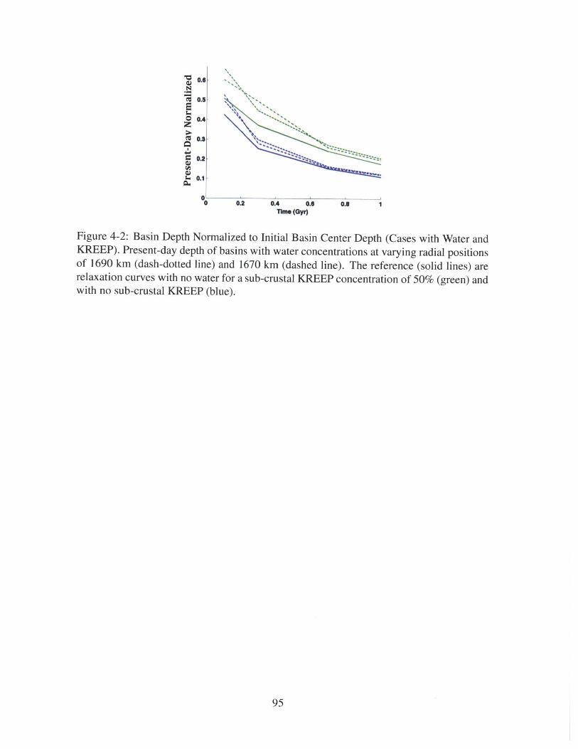
0.6-

0 0.4-

0.2

0.1

0 0.2 0.4 0.6 0.8 1Time (Gyr)

Figure 4-2: Basin Depth Normalized to Initial Basin Center Depth (Cases with Water andKREEP). Present-day depth of basins with water concentrations at varying radial positionsof 1690 km (dash-dotted line) and 1670 km (dashed line). The reference (solid lines) arerelaxation curves with no water for a sub-crustal KREEP concentration of 50% (green) andwith no sub-crustal KREEP (blue).

95

4.9 Tables

96

Table 4.1: Parameter Values for Impact Heating & Viscoelastic RelaxationParameter Value

Constant, a -0.31Constant, b 1.15

Constant, a, -0.346Constant, a2 -0.516Constant, b1 0.211Constant, b2 0.361

Mendel-Rydberg Rim Diameter 635 kmSlope of linear shock, S 1.20

Speed of Sound at STP, C 5.6 km/sVertical Projectile Velocity, vi 15 km/s

97

Chapter 5

Recovery of Buried Lunar Craters

5.1 Introduction

As a result of its accretionary history, the lack of a substantial atmosphere, and absence of

plate tectonics, the Moon is characterized by an extraordinarily well-preserved and mostly

ancient surface. With its accessibility to orbital and landed spacecraft that has provided

comprehensive global mapping as well as returned surface samples, the Moon has a unique

qualitative and quantitative role in understanding and constraining the evolution of our So-

lar System, as well as the timing of its many major events (e.g. (121)). The contrast of low

reflectance material of the lunar nearside maria against the high reflectance, anorthositic

highlands crust (107; 122) can be observed from Earth with the naked eye and is one of

the most recognizable features of the Moon. Geologic evidence supports the hypothesis

that the maria flooded the lunar nearside between 3.8-2.5 Gya, during at least three major

events (123). The emplacement of the lunar maria has obscured much of the original phys-

iographic expression of the nearside lowlands, nearly 20% of the entire surface (123; 122),

impairing our ability to fully understand this unique lunar region.

Previous workers have attempted to constrain the amount of maria emplaced on the lunar

surface using radar and seismic refraction data (124; 125; 126), localized gravity recovery

(127), geologic techniques relying on impact-exposed subsurface structure (128; 129), and

99

estimates based on partially buried (filled) craters (130; 131; 132; 123; 133). Some of these

investigations have provided insight into the history, average thickness, and age of the mare

flows and are summarized by (134). (135) and (136) suggest that the mare emplacement

represents the onset of a secondary crust, an expected outcome of terrestrial, planetary

bodies. Studies of basin mare deposits (129; 123) suggest the mare flooding of the eastern

lowlands occurred in three phases with an evolving Ti-content. While lenses of basin mare

fill have been approximated to be as much as 8.5-km thick (119; 133), the average mare

load for the lunar nearside is generally considered to be less than 2 km (130; 131; 132)

In this paper, we use gravity data acquired by the dual Gravity Recovery and Interior Lab-

oratory (GRAIL) spacecraft (137; 138; 58)in conjunction with altimetry data from the Lu-

nar Orbiter Laser Altimeter (LOLA) investigation (139; 140) on the Lunar Reconnaissance

Orbiter (141) to search for buried craters. We use this crater population in concert with

partially buried craters to investigate the average depth, volume, and density of lunar maria

that have been emplaced on the lunar nearside.

5.2 Data, Methodology & Modeling

5.2.1 Spherical Harmonic Localization

A real-valued, square-integrable function, g(Q), defined on a unit sphere can be expanded

as a linear combination of spherical harmonics (25) by

00 1

g() S S grmY1m(Q), (5.1)1=0 m=-1

and

film = j g(Q)Ym(Q)dQ, (5.2)

where Q is the solid angle, Yim is the spherical harmonic basis function of degree 1 and

order m, and glm are the corresponding spherical harmonic coefficients.

100

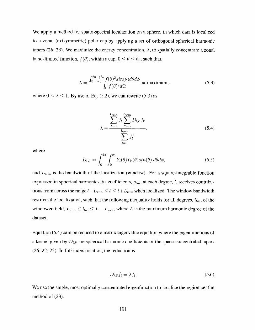
We apply a method for spatio-spectral localization on a sphere, in which data is localized

to a zonal (axisymmetric) polar cap by applying a set of orthogonal spherical harmonic

tapers (26; 23). We maximize the energy concentration, A, to spatially concentrate a zonal

band-limited function, f(0), within a cap, 0 < 0 < 00, such that,

07r f(O f(0)2si()~A - f fO f)sii()d~do maximum, (5.3)f2 f (0) 2dQ

where 0 < A < 1. By use of Eq. (5.2), we can rewrite (5.3) as

Lwin Lwin

Lwi

E f12l=0

where2,r 0

D,1 = j Y 1(0)Yp,(0)sin(0) d~d@, (5.5)

and Lwin is the bandwidth of the localization (window). For a square-integrable function

expressed in spherical harmonics, its coefficients, gim, at each degree, 1, receives contribu-

tions from across the range 1- Lin < 1 I+Lin when localized. The window bandwidth

restricts the localization, such that the following inequality holds for all degrees, 110, of the

windowed field, Lwin < 1ioc < L - Lwin, where L is the maximum harmonic degree of the

dataset.

Equation (5.4) cam be reduced to a matrix eigenvalue equation where the eigenfunctions of

a kernel given by Dy are spherical harmonic coefficients of the space-concentrated tapers

(26; 22; 23). In full index notation, the reduction is

D,1 f, = Af 1. (5.6)

We use the single, most optimally concentrated eigenfunction to localize the region per the

method of (23).

101

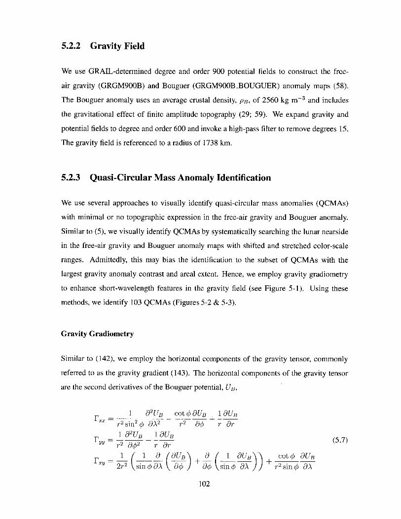
5.2.2 Gravity Field

We use GRAIL-determined degree and order 900 potential fields to construct the free-

air gravity (GRGM900B) and Bouguer (GRGM900BBOUGUER) anomaly maps (58).

The Bouguer anomaly uses an average crustal density, PB, of 2560 kg m-3 and includes

the gravitational effect of finite amplitude topography (29; 59). We expand gravity and

potential fields to degree and order 600 and invoke a high-pass filter to remove degrees 15.

The gravity field is referenced to a radius of 1738 km.

5.2.3 Quasi-Circular Mass Anomaly Identification

We use several approaches to visually identify quasi-circular mass anomalies (QCMAs)

with minimal or no topographic expression in the free-air gravity and Bouguer anomaly.

Similar to (5), we visually identify QCMAs by systematically searching the lunar nearside

in the free-air gravity and Bouguer anomaly maps with shifted and stretched color-scale

ranges. Admittedly, this may bias the identification to the subset of QCMAs with the

largest gravity anomaly contrast and areal extent. Hence, we employ gravity gradiometry

to enhance short-wavelength features in the gravity field (see Figure 5-1). Using these

methods, we identify 103 QCMAs (Figures 5-2 & 5-3).

Gravity Gradiometry

Similar to (142), we employ the horizontal components of the gravity tensor, commonly

referred to as the gravity gradient (143). The horizontal components of the gravity tensor

are the second derivatives of the Bouguer potential, UB,

= X 1 82 UB Cot #9UB IaUBr2 sin2 &A2 - r 2 (go r OrI a 2 UB 1aUB

FyY = - + a r+ (5.7)

1X = 1 ( OBs + 1 1 11UB ))+COt # allB

2r 2 sin 0 aA (90 a# sin 0 9A r 2 sin 0 9A

102

where r is the lunar radius, A is the longitude in radians, <5 is the colatitude in radians, and

x and y represent the longitudinal and latitudinal directions, respectively. As prescribed

by (142), we combine the horizontal gradient eigenvalues into a single value, Fhh, of the

second horizontal derivative of maximum amplitude at each Cartesian grid point on the

surface:

Phh F11 if 1711 > abs(7 2 2 ) (5.8)

F22 if F1 1 < abs(F 2 2 )

In addition, we employ a modified antieigenvalue to identify buried craters. The anti-

eigenvalue, [o, is defined as,

o AA 2 (5.9)A, + A2 '

and is valid for a positive-definite matrix (144). Accordingly, we modify the antieigenvalue

to be applicable for negative-definite matrices, with the following modification,

p = Re(Ipo) - AiA2 )+Im(2 A1A2) (5.10)A1 + A2

This is a novel approach to examine gravity fields and provides a tool to simultaneously

examine long- and short-wavelength structures without amplitude bias. We apply Eqns.

5.8-5.10, for the identification of QCMAs in the free-air gravity and Bouguer anomaly

fields.

Lunar Crater Relations

Assuming an initial, pre-impact site in isostasy with the surrounding area, we invoke the

following crater relation (Soderblom et al., in prep.), for Bouguer anomaly as a function of

crater diameter (Figure 5-5),

103

Ag_ = -0.2288D, + 9.1189

where Agu is the average gravity anomaly of the crater floor relative to the ejecta blanket

area, extending from the crater edge to 2-crater radii (145) and D, is the crater diameter.

We assume that D, is equivalent to the diameter of the QCMA.

Using a depth-diameter relation for fresh craters (Sori & Zuber, in prep.), we assume that

the average floor depths, d, of our filled craters are:

d = 2.57D 1 4 (5.12)

Similar to (Soderblom et al., in prep.), we average the Bouguer anomaly along the floor of

the putative buried craters (QCMAs) using (146) and (145),

0.19DI for Dc < 80 kmDf = (5.13)

Dc - 1.84 * DC/ 3 for D, > 80 km

where Df is the floor diameter. To prevent uplifted central peak material from influencing

our measurement in the central part of the crater, we use the floor diameter less the area

encompassed by the central peak diameter, Dc,, (147; 148),

0.22Dc for Dc < 140 kmD = (5.14)

0.4Dc for Dc > 140 km

with a central peak height, he,,

h min(3,0.0006D .97). (5.15)

For completely buried craters, we remove the influence of rim height from the depth of

the crater, as it will have a minimal influence on the gravity anomaly relative to the ejecta

104

(5.11)

blanket (see Figure 5-4).

hr = 0.236D 0. 3 9 9 (5.16)

5.2.4 Loading Model

In order to calculate the effects of material filling on the lunar nearside, we derive the

gravitational attraction of the mare load, Agm, at the surface, s, from the general form of

Newton's law of universal gravitation,

Ags = AgU + GApAh (5.17)E a2

e=1 e

where,

(P - pc for de< h - hf (5.18)

pl - pc for de > h - hf

and where pc is the density of the crust, pf is the density of the infill, h is the height of

the pre-impact surface above the floor, and hf is the height of the fill. Each element has an

area, Ae, height, he, depth below the pre-impact surface, de, and corresponding distance,

ae, between the element and measurement point on the reference surface, s. We choose to

discretize the load into a 101 x 101 x 101 element grid and use a local geoid surface grid of

101 x 101 elements.

5.2.5 Effective Density Estimation

Based on (40), we can calculate the effective density, pe, at the surface assuming a flat

surface (neglecting curvature) and crust-mantle boundary (41; 45),

1 - e-kho po APo 'Pe -k (5.19)

e ho (k k +d-1)

105

where k is the wavenumber, 2ho is the amplitude of topography, d is the depth of the

interface, po is the surface density, and Apo is the density contrast across the interface. The

above equation is formulated for a Cartesian grid without the finite-amplitude topography

correction.

For a set of density contrasts, we may compare the result from Eq. 5.19 to the topography-

induced gravity anomaly (LOLA 1080YAMWRP) from LOLA. We compute the admit-

tance spectrum over a localized region and compare with results from Eq. 5.19. The

transfer function relating the topography-induced gravity anomaly with unit density to the

Bouguer anomaly is the admittance spectrum, Z, defined as

Z(l) - Sgt(l) (5.20)Sit(l)

where Sgt is the cross-power spectrum of the Bouguer anomaly and topography-induced

gravity anomaly and Set is the power spectrum of the topography-induced gravity anomaly

(59).

5.3 Results & Discussion

5.3.1 Partially Buried Craters

We identify a population of 80 anomalously shallow craters on the lunar nearside that may

be partially buried by lunar maria. We limit our crater population to those within the lunar

maria region (see Figure 5-6) and with diameters of 20-200 km. Using Equation 5.11, we

can remove the portion of the gravity associated with crater formation and modification

(e.g. floor fracturing, mantle uplift) and use the remaining gravity anomaly to constrain the

density of the infill and excavated material (see Eq. 5.17, Fig. 5-7).

For our population of partially buried craters, we find a median density contrast of 100 kg-

m 3 (Fig. 5-7c) with a majority of the craters filled with material denser than the excavated

(original) surface. As shown in Fig 5-7, the excavated and fill density of the partially buried

106

craters have a bi-modal distribution with peaks at approximately 2400 and 3200 kg-m- 3

consistent with existence of two dominant mineralogies with different densities.

5.3.2 Buried Craters

We identify a population of 103 quasi-circular mass anomalies (QCMAs) on the lunar

nearside that may be craters filled by lunar maria (Fig 5-2). As shown in Figure 5-8a,

below 80-km diameter, a majority of the QCMAs are within one standard deviation of the

Bouguer anomaly mean for lunar craters. Beyond 80 km, the QCMAs concentrate into two

groups, one above and one below the average lunar crater trend.

We find the group of QCMAs above the lunar crater trend are most consistent with filled

material with an average density contrast of 800 kg/m 3, while the group below the trend are

best fit to a density contrast of -200 kg/m-3. This bi-modal distribution is consistent with

the histogram of density contrasts in Figure 5-8b.

5.3.3 Surface Depth & Volume Estimates

Using the existing lunar crater inventory for craters greater than 20 km (149) with the

QCMAs found in this study, we estimate variable depths and total volume of the lunar

nearside maria.

Crater-based Estimates

We focus on three main estimates using buried craters:

1. Scenario A - a depth calculation using depth differences between fresh craters and

regional lunar craters (including QCMAs).

2. Scenario B - a depth calculation using depth differences between fresh craters and

all buried craters.

107

3. Scenario C - a depth calculation using buried crater rim heights in addition to depth

differences between fresh craters and partially buried craters.

Scenario A presumes that any departure in crater depth from the pre-impact surface is due

to mare infill. We use the fresh crater depth-to-diameter relation (Eq. 5.12) less the rim

height (Eq. 5.16) to determine the expected depth, de. As the putative buried craters,

QCMAs, have minimal or no surface expression, we consider the craters and related rims

to be buried. Thus for the QCMAs, we use only the fresh crater depth-to-diameter relation

(Eq. 5.12) to approximate the mare fill height. Under this scenario, we find 3 x 107 km3 of

mare material, equivalent to a 3-km average layer, may be deposited on the lunar nearside

with lenses of material greater than 5-km depth (Fig. 5-9a).

With Scenario B, we also find a mare volume estimate of 3 x 107 km3, although this scenario

has a greater uniformity in depth across the lunar nearside (Fig. 5-9b). Scenario B presumes

the complete filling of craters is representative of the lunar nearside. In Scenario C, we

consider the complete filling of craters as non-representative of the region and assume the

major contribution of mare infill is partial crater infill and crater rim burial. For Scenario C,

we find a mare volume estimate of 2 x 107 km 3, equivalent to a 2-km layer of mare across

the lunar nearside region.

Localized Regional Analysis

Using localized admittance, we attempt to place constraints on the depth of mare fill for the

lunar nearside. With Equation 5.19, we consider the difference in the admittance profile

expected for a positive (increasing density with depth) and negative density (decreasing

density with depth). contrast at depth. From Figure 5-10, we expect a positive density

contrast to result in a monotonically decreasing curve and a negative density contrast to

result in a monotonically increasing curve.

We examine four lunar regions with localized admittance analysis, two with and two with-

out mare fill. In the regions without mare fill (see Figure 5-11), we observe a trend con-

sistent with a positive density contrast and a best-fit depth of 0 km. Contrarily, the regions

108

with mare fill have the opposite trend (see Figure 5-12) at higher harmonic degrees (>250),

with an increasing trend with harmonic degree. This is consistent with a denser layer being

present at the surface. Using Equation 5.19, we attempt to find a best-fit depth, but our

results are inconclusive, though would be consistent with depths of 0-8 km.

5.4 Discussion

5.4.1 Density

Our population of partially and putative buried craters provide constraints on the density of

mare material on the lunar nearside. Unlike completely buried craters, the partially buried

craters allow us to individually solve for the crater infill and excavated density (see Eq.

5.18). The multimodal distribution of partially buried crater excavated and fill densities

with peaks at the same densities suggest that two distinct mineralogies may be present.

The two peaks at approximately 2350 kg/m3 and 3150 kg/m 3 are consistent with fractured

anorthositic highlands crust and lunar maria densities (59; 127; 150).

The density contrast for the partially buried craters, centered at 100 kg/m 3 suggests, on

average, these craters tend to be filled with material of slightly denser material. This may

be due to a combination of crater fill by impact ejecta and mass wasting of the crater walls.

Further, this result suggests that mare fill of the anorthositic crust is rare and is unlikely

to provide a representative example of maria thickness on the lunar nearside. However,

we note our partially buried craters are biased toward craters along the periphery of the

nearside lunar maria region and crater rims and we may be preferentially selecting regions

where we are most likely to find anorthositic crustal impacts.

For our putative buried impact craters, we find that below 80-km diameter, craters have

the same Bouguer anomaly-to-diameter relationship as unfilled craters. This may indicate

that the majority of buried craters with less than 80-km diameter have impacted into mare,

without penetrating to an underlying crust, and are subsequently filled by mare of approx-

imately the same density. Beyond 80-km diameter, the Bouguer anomaly of the putative

109

craters diverge into a group with a high Bouguer anomaly, requiring an average density

contrast of 800 kg/m3 , and a group with a low Bouguer anomaly, requiring a density con-

trast less than -200 kg/m 3 . The low Bouguer anomaly group may be explained by an impact

into anorthositic crust overlain by mare that was subsequently re-filled by mare with the ex-

pected post-impact inflow to be of anorthositic crust and contributing to a lower Bouguer

anomaly. Additionally, the higher density of impact ejecta from a mare impact would con-

tribute to a low Bouguer anomaly. The high Bouguer anomaly group, is consistent with a

fill-to-excavated density contrast of approximately 800 kg/M3. This is the average density

contrast that we expect for an impact into anorthositic crust that was subsequently filled by

mare. Accordingly, the high Bouguer anomaly group may represent the pre-mare surface

of the lunar nearside. Given the error in the Bouguer anomaly-to-diameter relation, we

estimate the density contrast is 800±200 kg/m 3 with a lunar mare density of 3300±200

kg/m 3.

While our estimate of the lunar mare density is consistent with recent measurements (150)

of Apollo-era samples and lunar meteorites, our result may indicate slightly higher (100

kg/M3) bulk densities for the lunar maria or that the nearside lunar crust is less dense than

the average crust. This suggests that the lunar maria in buried craters may have a lower

porosity than the lunar samples, which could be explained by an extensive, less Ti-rich

lunar mare phase succeeding an earlier, Ti-rich phase as suggested by (123). This would

require a majority of our buried crater population to be filled by the early, Ti-rich lunar

mare phase.

5.4.2 Mare Depth & Volume

The divergence from the putative buried craters from the nominal Bouguer anomaly-to-

diameter trend occurs for between 50-80 km in diameter and likely corresponds to pene-

tration through lunar maria. Using (110), D = 1.32Df08 6D -0.086 where D,, represents

the single-to-complex transition diameter, approximately 20 km, and the excavation depth

as approximately 10% of the excavation diameter (145), the 50 to 80-km transition corre-

110

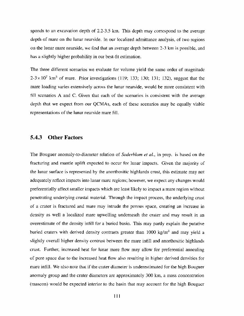
sponds to an excavation depth of 2.2-3.5 km. This depth may correspond to the average

depth of mare on the lunar nearside. In our localized admittance analysis, of two regions

on the lunar mare nearside, we find that an average depth between 2-3 km is possible, and

has a slightly higher probability in our best-fit estimation.

The three different scenarios we evaluate for volume yield the same order of magnitude

2-3x 10' km3 of mare. Prior investigations (119; 133; 130; 131; 132), suggest that the

mare loading varies extensively across the lunar nearside, would be more consistent with

fill scenarios A and C. Given that each of the scenarios is consistent with the average

depth that we expect from our QCMAs, each of these scenarios may be equally viable

representations of the lunar nearside mare fill.

5.4.3 Other Factors

The Bouguer anomaly-to-diameter relation of Soderblom et al., in prep. is based on the

fracturing and mantle uplift expected to occur for lunar impacts. Given the majority of

the lunar surface is represented by the anorthositic highlands crust, this estimate may not

adequately reflect impacts into lunar mare regions; however, we expect any changes would

preferentially affect smaller impacts which are least likely to impact a mare region without

penetrating underlying crustal material. Through the impact process, the underlying crust

of a crater is fractured and mare may intrude the porous space, creating an increase in

density as well a localized mare upwelling underneath the crater and may result in an

overestimate of the density infill for a buried basin. This may partly explain the putative

buried craters with derived density contrasts greater than 1000 kg/m3 and may yield a

slightly overall higher density contrast between the mare infill and anorthositic highlands

crust. Further, increased heat for lunar mare flow may allow for preferential annealing

of pore space due to the increased heat flow also resulting in higher derived densities for

mare infill. We also note that if the crater diameter is underestimated for the high Bouguer

anomaly group and the crater diameters are approximately 300 km, a mass concentration

(mascon) would be expected interior to the basin that may account for the high Bouguer

111

anomaly (Neumann, et al., in rev.)

5.5 Summary

Using gravity data from the GRAIL mission, we find 103 quasi-circular mass anomalies be-

neath the lunar nearside maria. Below 80 km, the mass anomalies follow the same Bouguer

anomaly-to-diameter trend as lunar craters, while they diverge at larger diameters, which

we have interpreted as impact craters exceeding the average depth of the lunar maria. With

separate analyses, using localized admittance and crater-based estimates, we constrain the

average thickness of the lunar maria to 2-3.5 km, or 2-3.5 x 107 km3 in total. The existence

of such a large quantity of buried craters suggests that there is a heterogeneous distribution

of lunar maria across the nearside, with craters and rim burial more than 5 km of lunar mare.

In concert with 80 anomalously shallow lunar nearside craters, we find the lunar maria may

have a density contrast of 800 kg/m 3 with the anorthositic highlands crust, resulting in a

lunar mare density of 3300±200 kg/m 3.


This work was conducted as part of the GRAIL mission and is supported by NASAs Dis-

covery Program and is performed under contract to the Massachusetts Institute of Tech-

nology and the Jet Propulsion Laboratory, California Institute of Technology. I thank J.

Soderblom, P. B. James, Y. Tewelde, and J. Andrews-Hanna for assistance and helpful

comments.

5.7 Figures

112

a)

30060

200

30 100

0

0-100

-200-30

-80 -60 -40 -20 0 20 40 60 80Longitude

b)

160

30

0

0-30

-80 -60 -40 -20 0 20 40 60 80Longitude

Figure 5-1: Lunar Nearside Gravity. Superimposed craters (black) and quasi-circular massanomalies (magenta) are shown on the lunar nearside a) Bouguer anomaly and b) modifiedantieigenvalue maps.

113

I 2

400

10 n 23010

-20 * OX4_4

-30-100 -50 0 50 100

Longitude

Figure 5-2: Lunar Nearside Topography (km) with Superimposed QCMAs. The imageencompasses the maria-flooded, nearside region of our investigation. QCMAs (magenta)and regional lunar craters (white) are shown with circles corresponding to the diameter.QCMAs more than 25 mgal above (circle) and below (square) the average crater Bougueranomaly v. diameter (see Eq. 5.11) are identified with black symbols.

114

a) b)

600 0

60

-1050_

50-2 40 -2

40 -3 -3-40 Loniu e -20 20 Lo30tude 40

70 300 300

200 60 200

100 1003 =50050 0 0

-100 40 -100

-200 -200-40 Lon iu9de -20 20 30 40Lgad Longitude 4

701 1

60

v60U3 =50

5040

400 0-40 Longii 9

ue -20 20 30 t0e 4Log~oeLongitude 4

Figure 5-3: Lunar Nearside Gravity. From top to bottom, panels of topography (km),Bouguer anomaly (mgal), and modified antieigenvalue. Superimposed craters (black) andquasi-circular mass anomalies (magenta) are shown antieigenvalue maps. a) Panels north-west of Imbrium basin. b) Panels northeast of Imbrium basin.

115

a)

Pm

b)

C)

Pm Pm

Figure 5-4: Conceptual Model (not to scale) a) Pre-Impact - The initial, pre-impact sur-

face (red-dashed line) is assumed to be in isostasy with the surrounding area with the

crustal layer (black) with density, pc above the upper mantle layer (white) with density

Pm. b) Post-impact modification, the crust is deformed leaving an unfilled crustal cavity

with impact-related fracturing and possible mantle uplift below the cavity. c) The impact

crater is subsequently filled partially or fully with the gray material which we presume is

lunar maria of density pf ill.

116

S,I

50 100 150 200Diameter (km)

50 100 150 200Diameter (km)

Figure 5-5: Rolling Average by Crater Diameter (km). a) The 20-km rolling average (solidline) and ±l- (dashed lines) for crater Bouguer anomaly (mgal), excluding the South-PoleAitken basin. b) Rolling average of density error based on I -- error of crater Bougueranomaly.

117

a)

100

2 80E

60

40

20

S0

-20

-40

-60

8 -80

-100

b)

500

450

400

-350E

S300

c 250

200

S150

100

50

0

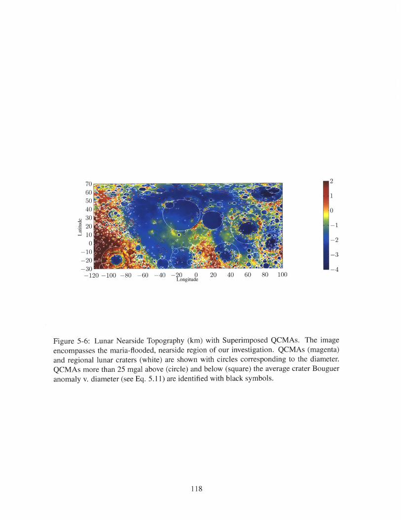
1)706015040 0

S3020-110

0 -20-10 --3

-30 -4-120 -100 -80 -60 -40 -20 0 20 40 60 80 100

Longitude

Figure 5-6: Lunar Nearside Topography (km) with Superimposed QCMAs. The image

encompasses the maria-flooded, nearside region of our investigation. QCMAs (magenta)

and regional lunar craters (white) are shown with circles corresponding to the diameter.

QCMAs more than 25 mgal above (circle) and below (square) the average crater Bouguer

anomaly v. diameter (see Eq. 5.11) are identified with black symbols.

118

c)

.4 I'1 0

CC

U

25

20

15

10

5

50 100 150 200Diameter (km)

0 I - - - __

2000 2500 3000 3500Excavated (Crustal) Density (kg/m3 )

0 ****UEUUUEEUE-500 0 500

Density Contrast (kg/M3 )

d)

12

10

0

8

6

4

2

0 L2000 2500 3000

Fill Density (kg/m3 )

1000

3500

Figure 5-7: Partially-Buried Craters Densities using GRAIL Data. a). The density contrastbetween the infill density and the excavated (pre-impact surface) density for the excessmaterial in partially buried crater. b) Crater count for partially-buried craters with thecalculated excavated density. c) Crater count for partially-buried craters with the calculateddensity contrast between the infill density and the excavated density. d) Crater count forpartially-buried craters across infill density.

119

a)

1000

800

600

400

200

0

-200

-400

-600

-800

-1000

0

b)

12

10 I

0Q

C)CC

Q

8

6

4

2

..

'

a)

200

-0 50-.'

100 --- --

50

0 0 JL

50 100 150 200Crater Diameter (kin)

b)

25

20

E 15

2004

3 10.

-500 0 500 1000Density Contrast (kg/rn3)

Figure 5-8: QCMA Trends using GRAIL Data. a) Normalized Average Bouguer Anomaly(mgal) v. Diameter (ki). Assuming the QCMAs are buried craters, gravity anomaly is

reference to the gravity anomaly within the ejecta blanket area. QCMAs (magenta circles)and lunar crater catalog (black dots) are shown with circles corresponding to diameter.QCMAs more than 25 mgal above (blue asterisks) and below (green asterisks) the normal-ized average crater Bouguer anomaly v. diameter. The lines are from Equation 5.17 withdensity contrasts of -200 (red-dashed), 0 (red solid), 200 (cyan dashed), 400 (cyan solid),600 (cyan dashed-dot), and 800 (red dashed-dot) kg/in 3 . b) Crater Count v Density Con-trast (kg/in3). The density contrast between the infill density and the excavated (pre-impactsurface) density for the excess material in partially buried crater.

120

(a)

-o

QLongitude

(b)

(c)

60

30

-301

-10

60.

30

0-

-30-

-100

-50 0Longitude

-50 QLongitude

50 100

50 100

5

4

3

2

1

10

0

,3

2

1

0

Figure 5-9: Nearside Mare Fill Depth Estimates (km). (a) Maximum Depth. This scenariois calculated based on interpolated differences of regional craters depths to reference freshcrater depths. (b) Completely and Partially Buried Crater Depth. This scenario is calcu-lated based on interpolated differences of completely and partially buried craters depthsto reference fresh crater depths. (c) Completely Buried Crater Rim Height and PartiallyBuried Crater Depths. This scenario is calculated based on completely buried crater rimheights and partially buried craters depths to reference fresh crater depths.

121

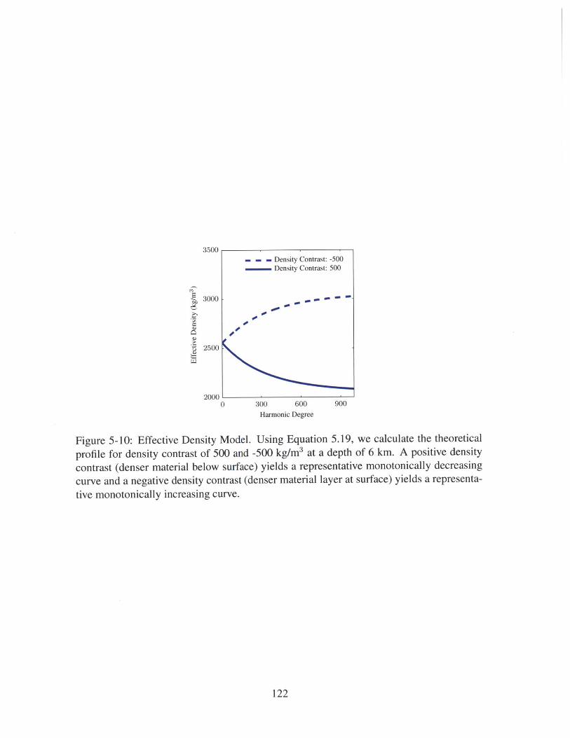
3500 , D C. . . Density Contrast: -500

....-Density Contrast: 500

- 3000 , . -

250020000

0 300 600 900

Harmonic Degree

Figure 5-10: Effective Density Model. Using Equation 5.19, we calculate the theoretical

profile for density contrast of 500 and -500 kg/m3 at a depth of 6 km. A positive density

contrast (denser material below surface) yields a representative monotonically decreasing

curve and a negative density contrast (denser material layer at surface) yields a representa-

tive monotonically increasing curve.

122

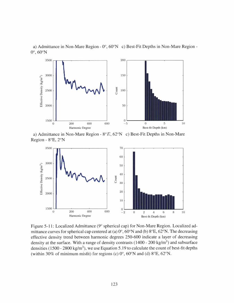
a) Admittance in Non-Mare Region - 0', 600N0", 60ON

c) Best-Fit Depths in Non-Mare Region -

C

3500

3000

2500

2000

1500 L0

a) Admittance inRegion - 80E, 20N

200 400 600Harmonic Degree

Non-Mare Region - 80E,

200

C

0

150

100

50

I1

0 L.-5 0 5 10

Best-fit Depth (km)

62 0N c) Best-Fit Depths in Non-Mare

200 400Harmonic Degree

70

C

0

60

50

40

30

20

10

6600 -2 0 2 4 6Best-fit Depth (km)

Figure 5-11: Localized Admittance (90 spherical cap) for Non-Mare Region. Localized ad-mittance curves for spherical cap centered at (a) 00, 60 0N and (b) 80E, 620N. The decreasingeffective density trend between harmonic degrees 250-600 indicate a layer of decreasingdensity at the surface. With a range of density contrasts (1400 - 200 kg/M3) and subsurfacedensities (1500 - 2800 kg/m3), we use Equation 5.19 to calculate the count of best-fit depths(within 30% of minimum misfit) for regions (c) 00, 60ON and (d) 80E, 62 0N.

123

3500

3000

2500 -

2000

6b

15000 8 10

. . . . .

.' '

---

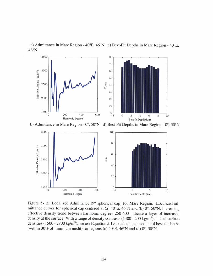
a) Admittance in Mare Region - 401E, 461N460N

c) Best-Fit Depths in Mare Region - 400E,

3500

U

LI~

3000

2500

2000

1500 L _ I0

b) Admittance in

200 400 600Harmonic Degree

Mare Region - 00, 50ON

80

70

C

0

60

50 -

40

30

20

10

-2 0 2 4 6 8Best-fit Depth (km)

d) Best-Fit Depths in Mare Region

200 400

Harmonic Degree

C

0

600

100

80

60

40

20

0'-5 0 5

Best-fit Depth (km)

Figure 5-12: Localized Admittance (90 spherical cap) for Mare Region. Localized ad-mittance curves for spherical cap centered at (a) 400E, 460N and (b) 00, 50 0 N. Increasingeffective density trend between harmonic degrees 250-600 indicate a layer of increaseddensity at the surface. With a range of density contrasts (1400 - 200 kg/M3) and subsurfacedensities (1500 - 2800 kg/m3 ), we use Equation 5.19 to calculate the count of best-fit depths(within 30% of minimum misfit) for regions (c) 400E, 460N and (d) 00, 50'N.

124

10

- 00, 50 0N

C

E

3500

3000

2500

2000

1500 -0I

10

. . . .

. .

01 -

Chapter 6

Future Work

6.1 A Wet Lunar Mantle: Basin Modification

The uncertainty in the initial basin depth profile we use for our lunar basin relaxation

model is possibly a large contribution to the error. The hydrodynamic simulation work

of Miljkovic et al., (in revision) may be used to constrain the uncertainty in our initial pro-

file for a variety of thermal conditions. This would also allow the investigation of long-term

viscoelastic basin relaxation modeling for nearside and lunar highland impacts. In addition

to impacts within the lunar highlands, inventories of young complex craters and basins

can help place constraints on viscosities and temperatures in our relaxation model as these

impact structures should exhibit less relaxation compared with the remainder of the lunar

basin inventory.

Using lunar elevation data, an average basin profile may be constructed and compared to

my model results to find the best-fit model. A best-fit analysis may then be used to con-

strain the water concentration for the upper lunar mantle. This analysis may be applied

the lunar impact basin inventory to identify possible lateral and temporal subsurface het-

erogeneities. Future work should also examine the effect of stress-dependent viscosity on

basin relaxation.

125

6.2 Recovery of Buried Lunar Craters

The inventory for partially buried craters is anomalously shallow craters on the lunar near-

side, mostly near the periphery of the lunar maria; this selection bias may skew our results.

Given the lack of statistically significant peaks in excavated and fill density plots, work

should be done to tailor the partially buried crater dataset to partially buried craters with

infill identified by spectral or imagery analysis. An analytical approach should be used to

determine the minimum infill density and depth required to uniquely attain accurate and

precise densities from best-fit analyses. This analysis may then be applied to use the best

crater candidates for the partially buried inventory.

Additionally, future work on this project should entail examination of the crater-size fre-

quency distribution with the buried crater population to place limits on the age of the near-

side mare region and underlying surface. This may provide further constraints on lunar

maria timing as well as a maximum age for the underlying surface.

The current analysis of buried craters does not consider overburied basins, which may be a

contributing factor to the lack of a characteristic density contrast peak consistent with lunar

maria density. A general error analysis may be conducted to constrain the density estimate

for a range of overburial values, although a best-fit analysis for a range of density contrasts

of buried basins may provide a more precise estimate.

The final partially and completely buried crater databases should be compared with con-

centrations of FeO, Th, and TiO 2 to ascertain any correlations in crater density with surface

deposits or increased heating. In general, statistical significance tests for my density and

mare thickness estimates should be applied to the results.

126

Bibliography

[1] L. Elkins-Tanton, S. Burgess, and Q.-Z. Yin, "The lunar magma ocean: Reconcil-ing the solidification process with lunar petrology and geochronology," Earth AndPlanetary Science Letters, vol. 304, pp. 326-336, Apr. 2011.

[2] D. H. Scott, K. L. Tanaka, and P. Geology, "Geologic map of the western equatorialregion of Mars, Scale 1:15,000,000, ," U.S. Geol. Survey Map I-1802-A., 1986.

[3] R. Greeley and J. Guest, "Geologic map of the eastern equatorial region of Mars,"Scale 1:15,000,000, U.S. Geol. Survey Map I-1802-B, 1987.

[4] G. E. McGill and S. W. Squyres, "Origin of the Martian crustal dichotomy: Evalu-ating hypotheses," Icarus, vol. 93, pp. 386-393, Oct. 1991.

[5] H. Frey, S. E. Sakimoto, and J. Roark, "The MOLA Topographic signature at thecrustal dichotomy boundary zone on Mars," Geophysical Research Letters, vol. 25,no. 24, pp. 4409-4412, 1998.

[6] D. E. Smith, "The Global Topography of Mars and Implications for Surface Evolu-tion," Science, vol. 284, pp. 1495-1503, May 1999.

[7] D. E. Smith, M. T. Zuber, H. V. Frey, J. B. Garvin, J. W. Head, D. 0. Muhle-man, G. H. Pettengill, R. J. Phillips, S. C. Solomon, H. J. Zwally, W. B. Banerdt,T. C. Duxbury, M. P. Golombek, F. G. Lemoine, G. A. Neumann, D. D. Rowlands,0. Aharonson, P. G. Ford, A. B. Ivanov, C. L. Johnson, P. J. McGovern, J. B. Ab-shire, R. S. Afzal, and X. Sun, "Mars Orbiter Laser Altimeter: Experiment summaryafter the first year of global mapping of Mars," Journal of Geophysical Research,vol. 106, pp. 23689-23722, Oct. 2001.

[8] M. Zuber, S. Solomon, R. Phillips, D. Smith, G. Tyler, 0. Aharonson, G. Balmino,W. Banerdt, J. Head, and C. Johnson, "Internal structure and early thermal evolutionof Mars from Mars Global Surveyor topography and gravity," Science, vol. 287,no. 5459, p. 1788, 2000.

[9] G. A. Neumann, M. T. Zuber, M. A. Wieczorek, P. J. McGovern, F. G. Lemoine,and D. E. Smith, "Crustal structure of Mars from gravity and topography," Journalof Geophysical Research-Planets, vol. 109, no. E8, p. E08002, 2004.

[10] W. Kiefer, "Buried mass anomalies along the hemispheric dichotomy in eastern

127

Mars: Implications for the origin and evolution of the dichotomy," Geophysical Re-search Letters, vol. 32, no. 22, p. L22201, 2005.

[11] B. Hynek and R. Phillips, "Evidence for extensive denudation of the Martian high-lands," Geology, vol. 29, no. 5, pp. 407-410, 2001.

[12] M. C. Malin, "Sedimentary Rocks of Early Mars," Science, vol. 290, pp. 1927-1937,Dec. 2000.

[13] R. A. Craddock, T. A. Maxwell, and A. D. Howard, "Crater morphometry and mod-ification in the Sinus Sabaeus and Margaritifer Sinus regions of Mars," Journal ofGeophysical Research-Planets, vol. 102, no. E6, pp. 13321-13340, 1997.

[14] R. A. Craddock and T. A. Maxwell, "Geomorphic evolution of the Martian high-lands through ancient fluvial processes," Journal of Geophysical Research-Planets,vol. 98, no. E2, pp. 3453-3468, 1993.

[15] M. P. Golombek, J. A. Grant, L. S. Crumpler, R. Greeley, R. E. Arvidson, J. F.Bell, III, C. M. Weitz, R. Sullivan, P. R. Christensen, L. A. Soderblom, and S. W.Squyres, "Erosion rates at the Mars Exploration Rover landing sites and long-termclimate change on Mars," Journal of Geophysical Research, vol. 111, pp. E12S 10-,Dec. 2006.

[16] C. I. Fassett and J. W. Head, III, "Layered mantling deposits in northeast ArabiaTerra, Mars: Noachian-Hesperian sedimentation, erosion, and terrain inversion,"Journal of Geophysical Research, vol. 112, p. E08002, Aug. 2007.

[17] J. M. Moore, "Nature of the mantling deposit in the heavily cratered terrain of north-eastern Arabia, Mars," Journal of Geophysical Research, vol. 95, no. B9, p. 14279,1990.

[18] M. T. Zuber, D. E. Smith, S. C. Solomon, D. 0. Muhleman, J. W. Head, J. B. Garvin,J. B. Abshire, and J. L. Bufton, "The Mars Observer laser altimeter investigation,"Journal of Geophysical Research-Planets, vol. 97, no. E5, pp. 7781-7797, 1992.

[19] A. Albee, R. Arvidson, F. Palluconi, and T. Thorpe, "Overview of the Mars GlobalSurveyor mission," Journal of Geophysical Research, 2001.

[20] R. W. Zurek and S. E. Smrekar, "An overview of the Mars Reconnaissance Orbiter(MRO) science mission," Journal of Geophysical Research, vol. 112, p. E05S01,May 2007.

[21] D. L. Turcotte, R. J. Willemann, W. F. Haxby, and J. Norberry, "Role of membranestresses in the support of planetary topography," Journal of Geophysical Research-Planets, vol. 86, no. B5, pp. 3951-3959, 1981.

[22] F. J. Simons, F. A. Dahlen, and M. A. Wieczorek, "Spatiospectral Concentration ona Sphere," SIAM Review, vol. 48, pp. 504-536, Jan. 2006.

[23] M. Wieczorek and F. Simons, "Localized spectral analysis on the sphere," Geophys-ical Journal International, vol. 162, no. 3, pp. 655-675, 2005.

128

[24] P. McGovern, S. Solomon, D. Smith, M. Zuber, M. Simons, M. Wieczorek,R. Phillips, G. Neumann, 0. Aharonson, and J. Head, "Localized gravity/topographyadmittance and correlation spectra on Mars: Implications for regional and globalevolution," Journal of Geophysical Research, vol. 107, no. 10.1029, 2002.

[25] M. Wieczorek, "The gravity and topography of the terrestrial planets," Treatise onGeophysics, vol. 10, pp. 165-206, 2007.

[26] F. J. Simons, "MATLAB Open Source Software," 2006.

[27] C. L. Johnson, J. W. Head, R. J. Phillips, D. E. Smith, and M. T. Zuber, "LithosphericLoading by the Northern Polar Cap on Mars," Icarus, vol. 144, pp. 313-328, Apr.2000.

[28] P. McGovern, S. Solomon, and D. Smith, "Correction to "Localized grav-ity/topography admittance and correlation spectra on Mars: Implications for regionaland global evolution"," Journal of Geophysical Research, vol. 109, pp. 1-5, 2004.

[29] M. A. Wieczorek and R. J. Phillips, "Potential anomalies on a sphere: Applica-tions to the thickness of the lunar crust," Journal of Geophysical Research-Planets,vol. 103, no. El, pp. 1715-1724, 1998.

[30] A. S. Konopliv, S. W. Asmar, W. M. Folkner, 0. Karatekin, D. C. Nunes, S. E.Smrekar, C. F. Yoder, and M. T. Zuber, "Mars high resolution gravity fields fromMRO, Mars seasonal gravity, and other dynamical parameters," Icarus, vol. 211,no. 1, pp. 401-428, 2011.

[31] J. C. Andrews-Hanna, M. T. Zuber, and W. B. Banerdt, "The Borealis basin andthe origin of the martian crustal dichotomy," Nature, vol. 453, pp. 1212-1215, June2008.

[32] M. H. Carr, "Mars Global Surveyor observations of Martian fretted terrain," Journalof Geophysical Research-Planets, vol. 106, no. E10, pp. 23571-23593, 2001.

[33] N. K. Forsberg-Taylor, "Crater degradation in the Martian highlands: Morphome-tric analysis of the Sinus Sabaeus region and simulation modeling suggest fluvialprocesses," Journal of Geophysical Research, vol. 109, no. E5, pp. 1-12, 2004.

[34] M. Carr, Water on Mars, vol. 326. Nature, Mar. 1987.

[35] G. E. McGill, "Crustal history of north central Arabia Terra, Mars," Journal of Geo-physical Research-Planets, vol. 105, no. E3, pp. 6945-6959, 2000.

[36] R. J. Phillips, "Ancient Geodynamics and Global-Scale Hydrology on Mars," Sci-ence, vol. 291, pp. 2587-2591, Mar. 2001.

[37] F. Nimmo and D. J. Stevenson, "Estimates of Martian crustal thickness from vis-cous relaxation of topography," Journal of Geophysical Research-Planets, vol. 106,no. E3, pp. 5085-5098, 2001.

[38] A. Crosby, "An assessment of the accuracy of admittance and coherence estimates

129

using synthetic data," Geophysical Journal International, vol. 171, no. 1, pp. 25-54,2007.

[39] D. Mckenzie, "Estimating Tein the presence of internal loads," Journal of Geophys-ical Research, vol. 108, no. B9, pp. 1-21, 2003.

[40] D. W. Forsyth, "Subsurface loading and estimates of the flexural rigidity of conti-nental lithosphere," Journal of Geophysical Research-Planets, vol. 90, pp. 12623-12632, Jan. 1985.

[41] D. Mckenzie, D. N. Barnett, and D.-N. Yuan, "The relationship between Martiangravity and topography," Earth And Planetary Science Letters, vol. 195, pp. 1-16,Jan. 2002.

[42] M. Grott and D. Breuer, "The evolution of the martian elastic lithosphere and impli-cations for crustal and mantle rheology," Icarus, vol. 193, pp. 503-515, Feb. 2008.

[43] T. Hoogenboom and S. Smrekar, "Elastic thickness estimates for the northern low-lands of Mars," Earth And Planetary Science Letters, vol. 248, pp. 830-839, Aug.2006.

[44] T. Watters, "Lithospheric flexure and the origin of the dichotomy boundary on Mars,"Geology, vol. 31, no. 3, pp. 271-274, 2003.

[45] F. Nimmo, "Admittance estimates of mean crustal thickness and density at the Mar-tian hemispheric dichotomy," Journal of Geophysical Research-Planets, vol. 107,no. E11, p. 5117, 2002.

[46] F. Nimmo, "Tectonic consequences of Martian dichotomy modification by lower-crustal flow and erosion," Geology, vol. 33, pp. 533-536, July 2005.

[47] T. R. Watters and P. J. McGovern, "Lithospheric flexure and the evolution ofthe dichotomy boundary on Mars," Geophysical Research Letters, vol. 33, no. 8,p. L08S05, 2006.

[48] S. Zhong and M. T. Zuber, "Long-wavelength topographic relaxation for self-gravitating planets and implications for the time-dependent compensation of surfacetopography," Journal of Geophysical Research-Planets, vol. 105, no. E2, pp. 4153-4164, 2000.

[49] E. M. Parmentier, D. L. Turcotte, and K. E. Torrance, "Studies of Finite AmplitudeNon-Newtonian Thermal Convection With Application to Convection in the Earth'sMantle," Journal of Geophysical Research, vol. 81, no. 11, pp. 1839-1846, 1976.

[50] A. G. W. Cameron and W. R. Ward, "Origin of the Moon," Lunar and PlanetaryInstitute Science Conference Abstracts, vol. 7, pp. 120-122, 1976.

[51] A. Cameron, "The Impact Theory for Origin of the Moon," Origin of the Moon,1986.

[52] R. M. Canup and E. Asphaug, "Origin of the moon in a giant impact near the end ofthe Earth's formation," Nature, vol. 412, no. 6848, pp. 708-712, 2001.

130

[53] R. M. Canup, "Dynamics of Lunar Formation," Annual review of astronomy andastrophysics, vol. 42, pp. 441-475, Sept. 2004.

[54] B. L. Jolliff, C. Floss, I. S. McCallum, and J. M. Schwartz, "Geochemistry petrologyand cooling history of 141617373 a plutonic lunar sample with textural evidence ofgranitic-fraction separation by silicate-liquid immiscibility," American Mineralogist,vol. 84, pp. 821-837, June 1999.

[55] J. A. Wood, J. S. Dickey, U. B. Marvin, and B. N. Powell, "Lunar Anorthosites,"Science, vol. 167, pp. 602-604, Jan. 1970.

[56] J. A. Wood, "Thermal history and early magmatism in the Moon," Icarus, vol. 16,pp. 229-240, Apr. 1972.

[57] P. Warren, "The magma ocean concept and lunar evolution," Annual Review of Earthand Planetary Sciences, 1985.

[58] M. T. Zuber, D. E. Smith, M. M. Watkins, S. W. Asmar, A. S. Konopliv, F. G.Lemoine, H. J. Melosh, G. A. Neumann, R. J. Phillips, S. C. Solomon, M. A. Wiec-zorek, J. G. Williams, S. J. Goossens, G. Kruizinga, E. Mazarico, R. S. Park, andD.-N. Yuan, "Gravity Field of the Moon from the Gravity Recovery and InteriorLaboratory (GRAIL) Mission," Science, vol. 339, pp. 668-671, Jan. 2013.

[59] M. A. Wieczorek, G. A. Neumann, F. Nimmo, W. S. Kiefer, G. J. Taylor, H. J.Melosh, R. J. Phillips, S. C. Solomon, J. C. Andrews-Hanna, S. W. Asmar, A. S.Konopliv, F. G. Lemoine, D. E. Smith, M. M. Watkins, J. G. Williams, and M. T.Zuber, "The Crust of the Moon as Seen by GRAIL," Science, vol. 339, pp. 671-675,Feb. 2013.

[60] P. C. Hess and E. M. Parmentier, "Thermal evolution of a thicker KREEP liquidlayer," Journal of Geophysical Research-Planets, vol. 106, pp. 28023-28032, Jan.2001.

[61] M. A. Wieczorek and R. J. Phillips, "The "Procellarum KREEP Terrane": Impli-cations for mare volcanism and lunar evolution," Journal of Geophysical Research-Planets, vol. 105, pp. 20417-20430, Aug. 2000.

[62] P. Lucey, R. L. Korotev, J. J. Gillis, L. A. Taylor, D. Lawrence, B. A. Campbell,R. Elphic, B. Feldman, L. L. Hood, D. Hunten, M. Mendillo, S. Noble, J. J. Papike,R. C. Reedy, S. Lawson, T. Prettyman, 0. Gasnault, and S. Maurice, "Understand-ing the Lunar Surface and Space-Moon Interactions," Reviews in Mineralogy andGeochemistry, vol. 60, pp. 83-219, 2006.

[63] K. Pahlevan and D. Stevenson, "Earth and Planetary Science Letters - Chemicalfractionation in the silicate vapor atmosphere of the Earth," Earth And PlanetaryScience Letters, vol. 301, pp. 433-443, 2011.

[64] C. Shearer, P. Hess, and M. Wieczorek, "Thermal and magmatic evolution of themoon," Reviews in Mineralogy and Geochemistry, 2006.

131

[65] A. E. Saal, E. H. Hauri, M. L. Cascio, J. A. Van Orman, M. C. Rutherford, and R. F.Cooper, "Volatile content of lunar volcanic glasses and the presence of water in theMoon's interior," Nature, vol. 454, pp. 192-195, July 2008.

[66] E. H. Hauri, T. Weinreich, A. E. Saal, M. C. Rutherford, and J. A. Van Orman, "HighPre-Eruptive Water Contents Preserved in Lunar Melt Inclusions," Science, vol. 333,pp. 213-215, July 2011.

[67] L. Elkins-Tanton and T. L. Grove, "Water (hydrogen) in the lunar mantle: Resultsfrom petrology and magma ocean modeling," Earth And Planetary Science Letters,vol. 307, pp. 173-170, 2011.

[68] J. P. Greenwood, S. Itoh, N. Sakamoto, P. Warren, L. Taylor, and H. Yurimoto,"Hydrogen isotope ratios in lunar rocks indicate delivery of cometary water to theMoon," Nature Geoscience, vol. 4, pp. 79-82, Jan. 2011.

[69] A. E. Saal, E. H. Hauri, J. A. Van Orman, and M. J. Rutherford, "D/H Ratios of theLunar Volcanic Glasses," in Lunar and Planetary Science Conference Proceedings,p. 2, 2012.

[70] P. H. Warren and J. T. Wasson, "The origin of KREEP," Reviews of Geophysics,vol. 17, no. 1, pp. 73-88, 1979.

[71] G. Hirth and D. L. Kohlstedt, "Experimental constraints on the dynamics of the par-tially molten upper mantle, 2, Deformation in the dislocation creep regime," Journalof Geophysical Research, vol. 100, no. B8, pp. 15441-15449, 1995.

[72] G. Neumann, M. Zuber, D. Smith, and F. Lemoine, "The lunar crust: Globalstructure and signature of major basins," Journal of Geophysical Research-Planets,vol. 101, no. E7, pp. 16841-16863, 1996.

[73] L. L. Hood and M. T. Zuber, "Recent Refinements in Geophysical Constraints onLunar Origin and Evolution," Origin of the Earth and Moon, pp. 397-409, 2000.

[74] D. Bercovici and S.-i. Karato, "Whole-mantle convection and the transition-zonewater filter," Nature, vol. 425, pp. 39-44, Sept. 2003.

[75] J. G. Williams, A. Konopliv, D. Boggs, R. S. Park, D. Yuan, F. G. Lemoine, S. J.Goossens, E. Mazarico, F. Nimmo, R. Weber, S. W. Asmar, H. J. Melosh, G. A. Neu-mann, R. J. Phillips, D. E. Smith, S. C. Solomon, M. M. Watkins, M. A. Wieczorek,J. Andrews-Hanna, J. W. Head, III, W. S. Kiefer, I. Matsuyama, P. J. McGovern,G. J. Taylor, and M. T. Zuber, "Lunar Interior Properties From the Grail Mission,"Journal of Geophysical Research, to be submitted.

[76] I. Garrick-Bethell, B. P. Weiss, D. L. Shuster, and J. Buz, "Early Lunar Magnetism,"Science, vol. 323, pp. 356-359, Jan. 2009.

[77] C. Cournede, J. Gattacceca, and P. Rochette, "Magnetic study of large Apollo sam-ples: Possible evidence for an ancient centered dipolar field on the Moon," EarthAnd Planetary Science Letters, vol. 331-332, pp. 31-42, May 2012.

132

[78] E. K. Shea, B. P. Weiss, W. S. Cassata, D. L. Shuster, S. M. Tikoo, J. Gattacceca,T. L. Grove, and M. D. Fuller, "A long-lived lunar core dynamo.," Science, vol. 335,pp. 453-456, Jan. 2012.

[79] C. Suavet, B. P. Weiss, W. S. Cassata, D. L. Shuster, J. Gattacceca, L. Chan,I. Garrick-Bethell, J. W. Head, T. L. Grove, and M. D. Fuller, "Persistence and ori-gin of the lunar core dynamo," Proceedings of the National Academy of Sciences,vol. 110, no. 21, pp. 8453-8458, 2013.

[80] S. K. Runcorn, "The formation of the lunar core," Geochimica et CosmochimicaActa, vol. 60, pp. 1205-1208, Apr. 1996.

[81] D. R. Stegman, A. Jellinek, S. Zatman, J. R. Baumgardner, and M. A. Richards,"An early lunar core dynamo driven by thermochemical mantle convection," Nature,vol. 421, no. 9 January 2003, pp. 143-146, 2003.

[82] M. Le Bars, M. A. Wieczorek, 0. Karatekin, D. Cebron, and M. Laneuville, "Animpact-driven dynamo for the early Moon," Nature, pp. 215-218, Oct. 2011.

[83] I. S. McCallum and J. M. Schwartz, "Lunar Mg suite: Thermobarometry and pet-rogenesis of parental magmas," Journal of Geophysical Research-Planets, vol. 106,pp. 27969-27983, Jan. 2001.

[84] J. Longhi and L. D. Ashwal, "Two-stage models for lunar and terrestrial anorthositesPetrogenesis without a magma ocean," Journal of Geophysical Research, vol. 15,pp. 571-14, Feb. 1985.

[85] D. Kohlstedt, "The Role of Water in High-Temperature Rock Deformation," Reviewsin Mineralogy and Geochemistry, 2006.

[86] L. Moresi and V. Solomatov, "Numerical investigation of 2D convection with ex-tremely large viscosity variations," Physics of Fluids, vol. 7, no. 9, pp. 2154-2162,1995.

[87] S. Zhong, M. T. Zuber, L. Moresi, and M. Gurnis, "Role of temperature-dependentviscosity and surface plates in spherical shell models of mantle convection," Journalof Geophysical Research, vol. 105, no. B5, pp. 11063-11082, 2000.

[88] J. Roberts and S. Zhong, "Plume-induced topography and geoid anomalies and theirimplications for the Tharsis rise on Mars," Journal of Geophysical Research, 2004.

[89] J. H. Roberts and S. Zhong, "Degree-1 convection in the Martian mantle and theorigin of the hemispheric dichotomy," Journal of Geophysical Research, 2006.

[90] J. Korenaga, "Scaling of stagnantlid convection with Arrhenius rheology and theeffects of mantle melting," Geophysical Journal International, vol. 179, pp. 154-170, 2009.

[91] S. Zhong, D. A. Yuen, and L.-N. Moresi, "Numerical methods for mantle convec-tion," Treatise on Geophysics, vol. 7, pp. 227-252, 2007.

133

[92] S. Zhong, E. M. Parmentier, and M. T. Zuber, "A dynamic origin for the globalasymmetry of lunar mare basalts," Earth And Planetary Science Letters, vol. 177,no. 3-4, pp. 131-140, 2000.

[93] W.-S. Yang and J. R. Baumgardner, "A matrix-dependent transfer multigrid methodfor strongly variable viscosity infinite Prandtl number thermal convection," Geo-physical & Astrophysical Fluid Dynamics, vol. 92, pp. 151-195, Nov. 2000.

[94] G. Hirth and D. L. Kohlstedt, "Water in the oceanic upper mantle: implications forrheology, melt extraction and the evolution of the lithosphere," Earth And PlanetaryScience Letters, vol. 144, no. 1-2, pp. 93-108, 1996.

[95] S. J. Mackwell, D. L. Kohlstedt, and M. S. Paterson, "The Role of Water in theDeformation of Olivine Single Crystals," Journal of Geophysical Research, vol. 90,no. B13, pp. 11319-11,333, 1985.

[96] R. S. Borch and H. W. Green, II, "Deformation of peridotite at high pressure in a newmolten salt cell: comparison of traditional and homologous temperature treatments,"Physics of The Earth and Planetary Interiors, vol. 55, pp. 269-276, June 1989.

[97] U. R. Christensen, V. Holzwarth, and A. Reiners, "Energy flux determines magneticfield strength of planets and stars," Nature, vol. 457, pp. 167-169, Jan. 2009.

[98] W. Konrad and T. Spohn, "Thermal history of the Moon: Implications for anearly core dynamo and post-accertional magmatism," Advances in Space Research,vol. 19, no. 10, pp. 1511-1521, 1997.

[99] J. G. Williams, D. H. Boggs, C. F. Yoder, J. T. Ratcliff, and J. 0. Dickey, "Lu-nar rotational dissipation in solid body and molten core," Journal of GeophysicalResearch-Planets, vol. 106, pp. 27933-27968, Jan. 2001.

[100] C. A. Dwyer, D. J. Stevenson, and F. Nimmo, "A long-lived lunar dynamo driven bycontinuous mechanical stirring," Nature, vol. 479, no. 7372, pp. 212-214, 2011.

[101] M. Fuller and S. M. Cisowski, "Lunar paleomagnetism.," Geomagnetism, vol. 2,pp. 307-455, 1987.

[102] S. M. Tikoo, B. P. Weiss, J. Buz, E. A. Lima, E. K. Shea, G. Melo, and T. L. Grove,"Magnetic fidelity of lunar samples and implications for an ancient core dynamo,"Earth And Planetary Science Letters, vol. 337-338, no. 0, pp. 93-103, 2012.

[103] A. Khan, A. Pommier, and J. A. D. Connolly, "On the Presence of a Titanium-RichMelt Layer in the Deep Lunar Interior," in Lunar and Planetary Science ConferenceProceedings, p. 2, 2013.

[104] C. K. Shearer and J. J. Papike, "Basaltic magmatism on the Moon: A perspectivefrom volcanic picritic glass beads," Geochimica et Cosmochimica Acta, vol. 57,pp. 4785-4812, 1993.

[105] L. T. Elkins, V. A. Fernandes, J. W. Delano, and T. L. Grove, "Origin of lunar ul-

134

tramafic green glasses: constraints from phase equilibrium studies," Geochimica etCosmochimica Acta, vol. 64, pp. 2339-2350, July 2000.

[106] R. Weber, P. Lin, E. Garnero, and Q. Williams, "Seismic Detection of the LunarCore," Science, 2011.

[107] D. E. Wilhelms and J. F. McCaulay, The Geology of the Moon. US Geol. Surv. Prof,1987.

[108] S. C. Solomon and J. Longhi, "Magma oceanography. I - Thermal evolution," Lu-nar and Planetary Science Conference Proceedings Abstracts, vol. 8, pp. 583-599,1977.

[109] S. Solomon, R. Comer, and J. W. Head, "The evolution of impact basins-Viscousrelaxation of topographic relief," Journal of Geophysical Research, vol. 87, no. B5,pp. 3975-3992, 1982.

[110] K. A. Holsapple, "The Scaling of Impact Processes in Planetary Sciences," AnnualReview of Earth and Planetary Sciences, vol. 21, pp. 333-373, Jan. 2013.

[111] K. K. Williams and M. T. Zuber, "Measurement and Analysis of Lunar Basin Depthsfrom Clementine Altimetry," Icarus, vol. 131, pp. 107-122, Jan. 1998.

[112] E. Pierazzo, A. M. Vickery, and H. J. Melosh, "A Reevaluation of Impact MeltProduction," Icarus, vol. 127, pp. 408-423, June 1997.

[113] W. S. Kiefer, P. J. McGovern, R. Potter, and G. S. Collins, "The Collapse of Super-Isostasy: The Thermal Evolution of Large Lunar Impact Basins and a Volcanic In-trusion Model for Lunar Mascon Gravity Anomalies," Lunar and Planetary ScienceConference Proceedings Abstracts, vol. 43, 2012.

[114] W. A. Watters, M. T. Zuber, and B. H. Hager, "Thermal perturbations caused by largeimpacts and consequences for mantle convection," Journal of Geophysical Research,vol. 114, no. E02001, pp. 1-23, 2009.

[115] T. J. Ahrens and J. D. Okeefe, "Equations of state and impact-induced shock-waveattenuation on the moon," Impact and explosion cratering: Planetary and terrestrialimplications; Proceedings of the Symposium on Planetary Cratering Mechanics,pp. 639-656, 1977.

[116] S. Zhong, A. Paulson, and J. Wahr, "Three-dimensional finite-element modelling ofEarth's viscoelastic deformation: effects of lateral variations in lithospheric thick-ness," Geophysical Journal of the Royal Astronomical Society, vol. 155, no. 2,pp. 679-695, 2003.

[117] P. Wu and W. R. Peltier, "Viscous gravitational relaxation," Geophysical Journal ofthe Royal Astronomical Society, vol. 70, no. 2, pp. 435-485, 1982.

[118] S. R. Bratt, S. C. Solomon, and J. W. Head, "The evolution of impact basins:Cooling, subsidence, and thermal stress," Journal of Geophysical Research-Planets,vol. 90, pp. 12415-12433, Jan. 1985.

135

[119] S. C. Solomon and J. W. Head, "Lunar Mascon Basins: Lava filling, tectonics, andevolution of the lithosphere," Reviews of Geophysics, vol. 18, no. 1, pp. 107-141,1980.

[120] E. Parmentier, S. Zhong, and M. T. Zuber, "Gravitational differentiation due to initialchemical stratification: origin of lunar asymmetry by the creep of dense KREEP?,"Earth And Planetary Science Letters, vol. 201, pp. 473-480, 2002.

[121] F. Tera, D. A. Papanastassiou, and G. J. Wasserburg, "Isotopic evidence for a termi-nal lunar cataclysm," Earth And Planetary Science Letters, vol. 22, no. 1, pp. 1-21,1974.

[122] B. L. Jolliff, J. J. Gillis, L. A. Haskin, R. L. Korotev, and M. A. Wieczorek, "Ma-jor lunar crustal terranes: Surface expressions and crust-mantle origins," Journal ofGeophysical Research-Planets, vol. 105, pp. 4197-4216, Jan. 2000.

[123] J. W. Head, "Lunar Mare Deposits: Areas, Volumes, Sequence, and Implication forMelting in Source Areas," LPI Contributions, vol. 234, p. 66, 1975.

[124] M. R. Cooper, R. L. Kovach, and J. S. Watkins, "Lunar near-surface structure," Re-views of Geophysics, vol. 12, no. 3, pp. 291-308, 1974.

[125] V. L. Sharpton and J. W. Head, III, "Stratigraphy and structural evolution of SouthernMare Serenitatis: A reinterpretation based on Apollo Lunar Sounder Experimentdata," Journal of Geophysical Research, vol. 87, no. B 13, p. 10983, 1982.

[126] T. Ono, A. Kumamoto, H. Nakagawa, Y. Yamaguchi, S. Oshigami, A. Yamaji,T. Kobayashi, Y. Kasahara, and H. Oya, "Lunar Radar Sounder Observations of Sub-surface Layers Under the Nearside Maria of the Moon," Science, vol. 323, pp. 909-912, Feb. 2009.

[127] M. Talwani, G. Thompson, B. Dent, H.-G. Kahle, and S. Buck, "Traverse GravimeterExperiment," Apollo 17: Preliminary Science Report, vol. 330, p. 13, 1973.

[128] C. J. Budney and P. G. Lucey, "Basalt thickness in Mare Humorum: The crater ex-cavation method," Journal of Geophysical Research, vol. 103, p. 16855, July 1998.

[129] B. J. Thomson, E. B. Grosfils, D. B. J. Bussey, and P. D. Spudis, "A new tech-nique for estimating the thickness of mare basalts in Imbrium Basin," GeophysicalResearch Letters, vol. 36, p. L12201, June 2009.

[130] R. A. DeHon and J. D. Waskom, "Geologic structure of the eastern mare basins,"Lunar and Planetary Science Conference Proceedings, vol. 7, pp. 2729-2746, Apr.1976.

[131] R. A. DeHon, "Thickness of the Western Mare Basalt," Proceedings of the Lunarand Planetary Science Conference 10th, pp. 2935-2955, 1979.

[132] F. H6rz, "How thick are lunar mare basalts," Lunar and Planetary Science Confer-ence Proceedings, vol. 9, pp. 3311-3331, 1978.

136

[133] J. W. Head, "Lava flooding of ancient planetary crusts: Geometry, thickness, andvolumes of flooded lunar impact basins," The Moon, vol. 26, pp. 61-88, Feb. 1982.

[134] H. Hiesinger, J. W. Head, U. Wolf, R. Jaumann, and G. Neukum, "Lunar mare basaltflow units: Thicknesses determined from crater size-frequency distributions," Geo-physical Research Letters, vol. 29, no. 8, pp. 891-894, 2002.

[135] J. W. Head, III and L. Wilson, "Lunar mare volcanism: Stratigraphy, eruption con-ditions, and the evolution of secondary crusts," Geochimica et Cosmochimica Acta,vol. 56, pp. 2155-2175, June 1992.

[136] J. L. Whitten and J. W. Head, III, "Detecting volcanic resurfacing of heavily crateredterrain: Flooding simulations on the Moon using Lunar Orbiter Laser Altimeter(LOLA) data," Planetary and Space Science VL, in press.

[137] A. S. Konopliv, R. S. Park, D.-N. Yuan, S. W. Asmar, M. M. Watkins, J. G. Williams,E. Fahnestock, G. Kruizinga, M. Paik, D. Strekalov, N. Harvey, D. E. Smith, andM. T. Zuber, "The JPL lunar gravity field to spherical harmonic degree 660 fromthe GRAIL Primary Mission," Journal of Geophysical Research-Planets, vol. 118,pp. 1415-1434, July 2013.

[138] F. G. Lemoine, S. Goossens, T. J. Sabaka, J. B. Nicholas, E. Mazarico, D. D. Row-lands, B. D. Loomis, D. S. Chinn, D. S. Caprette, G. A. Neumann, D. E. Smith,and M. T. Zuber, "High-degree gravity models from GRAIL primary mission data,"Journal of Geophysical Research-Planets, 2013.

[139] D. E. Smith, M. T. Zuber, G. B. Jackson, J. F. Cavanaugh, G. A. Neumann, H. Riris,X. Sun, R. S. Zellar, C. Coltharp, J. Connelly, R. B. Katz, I. Kleyner, P. Liiva, A. Ma-tuszeski, E. M. Mazarico, J. F. McGarry, A.-M. Novo-Gradac, M. N. Ott, C. Peters,L. A. Ramos-Izquierdo, L. Ramsey, D. D. Rowlands, S. Schmidt, V. S. Scott, G. B.Shaw, J. C. Smith, J.-P. Swinski, M. H. Torrence, G. Unger, A. W. Yu, and T. W.Zagwodzki, "The Lunar Orbiter Laser Altimeter Investigation on the Lunar Recon-naissance Orbiter Mission," Space Science Reviews, vol. 150, pp. 209-241, May2009.

[140] D. E. Smith, M. T. Zuber, G. A. Neumann, F. G. Lemoine, E. Mazarico, M. H.Torrence, J. F. McGarry, D. D. Rowlands, J. W. Head, T. H. Duxbury, 0. Aharonson,P. G. Lucey, M. S. Robinson, 0. S. Barnouin, J. F. Cavanaugh, X. Sun, P. Liiva, D.-d. Mao, J. C. Smith, and A. E. Bartels, "Initial observations from the Lunar OrbiterLaser Altimeter (LOLA)," Geophysical Research Letters, vol. 37, no. 18, p. L18204,2010.

[141] G. Chin, S. Brylow, M. Foote, J. Garvin, J. Kasper, J. Keller, M. Litvak, I. Mitro-fanov, D. Paige, K. Raney, M. Robinson, A. Sanin, D. Smith, H. Spence, P. Spudis,S. A. Stern, and M. Zuber, "Lunar Reconnaissance Orbiter Overview: The Instru-ment Suite and Mission," Space Science Reviews, vol. 129, no. 4, pp. 391-419, 2007.

[142] J. C. Andrews-Hanna, S. W. Asmar, J. W. Head, W. S. Kiefer, A. S. Konopliv,F G. Lemoine, I. Matsuyama, E. Mazarico, P. J. McGovern, H. J. Melosh, G. A.

137

Neumann, F. Nimmo, R. J. Phillips, D. E. Smith, S. C. Solomon, G. J. Taylor,M. A. Wieczorek, J. G. Williams, and M. T. Zuber, "Ancient Igneous Intrusions andEarly Expansion of the Moon Revealed by GRAIL Gravity Gradiometry," Science,vol. 339, pp. 675-678, Feb. 2013.

[143] G. B. Reed, "Application of kinematical geodesy for determining the short wavelength components of the gravity field by satellite gradiometry.," Reports of the De-partment of Geodetic Science, The Ohio State University, Mar. 1973.

[144] K. Gustafson, "Antieigenvalues," Linear Algebra and its Applications, vol. 208-209,pp. 437-454, Sept. 1994.

[145] H. J. Melosh, Impact Cratering: A Geologic Process. Oxford Monographs on Geol-ogy and Geophysics, Oxford University Press, 1989.

[146] R. J. Pike, "Apparent depth/apparent diameter relation for lunar craters," Lunar Sci-ence Conference Proceedings, vol. 3, pp. 3427-3436, 1977.

[147] R. J. Pike, "Some Morphologic Systematics of Complex Impact Structures," Mete-oritics, vol. 20, no. 1, pp. 49-68, 1985.

[148] C. A. Wood and J. W. Head, "Comparison of impact basins on Mercury, Mars andthe moon ," Lunar Science Conference Proceedings, vol. 3, pp. 3629-3651, 1976.

[149] J. W. Head, C. I. Fassett, S. J. Kadish, D. E. Smith, M. T. Zuber, G. A. Neumann, andE. Mazarico, "Global Distribution of Large Lunar Craters: Implications for Resur-facing and Impactor Populations," Science, vol. 329, pp. 1504-1507, Sept. 2010.

[150] W. S. Kiefer, R. J. Macke, D. T. Britt, and A. J. Irving, "Regional Variability inthe Density of Lunar Mare Basalts and Implications for Lunar Gravity Modeling,"Lunar and Planetary Science Conference Proceedings Abstracts, 2012.

138

Geophysical Evolution of Planetary Interiors and Surfaces: Moon ...

Documents

Transcript of Geophysical Evolution of Planetary Interiors and Surfaces: Moon ...