1

Geography or Politics? Regional Inequality in Colonial India

Keywords: South Asia, colonialism, regional inequality

JEL codes: N15, N95

Tirthankar Roy

London School of Economics and Political Science

t.oy@lse.ac.uk

September 2013

Abstract

Explaining regional inequality in the nineteenth century world forms a major

preoccupation of global history. A large country like India, being composed of

regions that differed in geographical and political characteristics, raises a parallel set

of issues to those debated in global economic history. With a new dataset, the paper

attempts to tackle these issues, and finds evidence to suggest that regional

differences, and divergence, were significantly influenced by geographical conditions.

2

3

Geography or Politics? Regional Inequality in Colonial India1

The divergence debate of the last decade has stimulated research on the

economic history of the non-European world. While trying to answer the broader

question, why Asia, Africa, or Latin America fell behind Europe in the nineteenth

century, the scholarship also emphasizes the heterogeneity of growth experiences

within the periphery. The heterogeneity is seen to derive from two sources,

colonialism and geography. European colonial rule, which was an agent in

institutional change, is believed to have produced diverse legacies on property rights

and public goods in the nations that attained freedom in the middle of the twentieth

century (Acemoglu, Johnson, Robinson, 2001; La Porta, Lopez-de-Silanes, Shleifer,

2008; Austin, 2008). Locally rooted factors such as natural resource endowments

are seen to have played a role too, either directly by shaping the ability of individual

regions to gain from trade, or indirectly by shaping competition for resources and

institutional outcomes of such competition (Sokoloff and Engerman, 2000; Sachs,

2003).

Deep heterogeneity in both these senses was present within a large peripheral

entity, India; so much so that the question why India stayed poor while Europe

became rich cannot have a single answer at all. The answer must depend on which

part of India one considers. How different were the Indian regions, why were they

different, and was the gap between them growing or narrowing in the era of colonial

rule? One reason to enter the subject is that the answers to these questions should

share parallels with the divergence discourse. Another reason arises from the

historiography of India. Historians have long acknowledged the need to study

regional differentiation to be able to qualify any general statement about economic

transformation in India. A review of the field observes that, ‘social and agricultural

regions both smaller and larger than provinces have increasingly seemed appropriate

units to scholars’ (Bayly, 1985, p. 584). Another overview notes that ‘South Asia

possessed a .. series of regional economies’ (Washbrook, 2001, p. 373). However, a

1 Acknowledgment: I wish to thank Shimon Agur who, with painstaking care, processed the Gazetteer dataset on which the paper is based. Comments and suggestions received on earlier versions from Latika Chaudhary, Bishnupriya Gupta, Kunal Sen, and Anand Swamy are gratefully acknowledged. I thank Steve Gibbons for helpful advice on the use of spatial regression tools on Stata. A version of the paper was read at the History and Economic Development Group workshop in the London School of Economics, 2012. I thank the participants for their comments.

4

shared strategy about how regional differentiation should be incorporated into

economic history did not exist until recently.

A recent scholarship has broken new ground by conducting quantitative

studies of regional inequality. It has found empirical support for the proposition that

present-day regional inequality owes to two particular colonial legacies, property

right and indirect rule. The paper is a re-examination of the issues raised in this

scholarship with the aid of new dataset, and reaches a different conclusion. In

particular, the role of natural resource conditions receives greater emphasis in the

present paper. The rest of the paper has six sections: the nature of regional

differentiation and interpretations thereof in the current literature, empirical

strategy, three sections on data analyses, and conclusion.

Historiography

The productive power and livelihood pattern of Indian regions differed greatly

around 1900. A district such as Bombay was possibly the most industrialized in the

contemporary tropical world. In the central Indian uplands, Chanda district had no

industry and only 15 per cent of its land under cultivation. The capital of this district,

which was as large in area as Belgium, was a town of 17,000 people. Both Bombay

and Chanda belonged in British India, but in very different geographical zones,

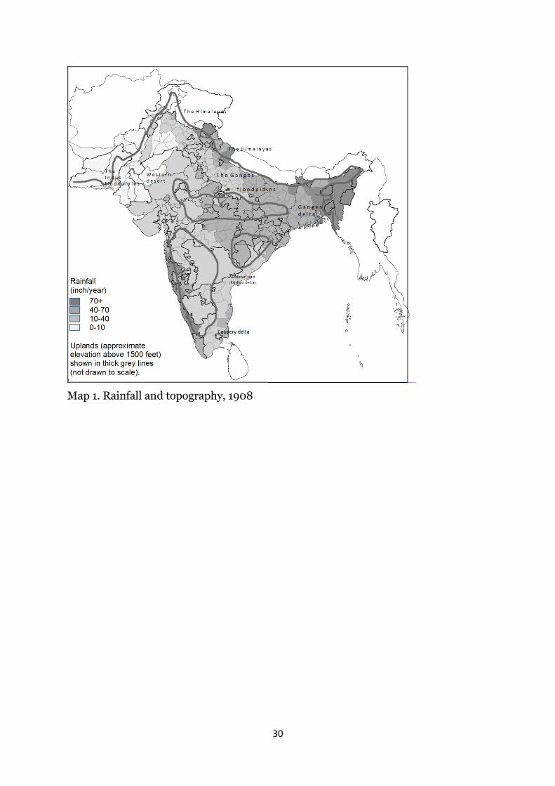
coastal-deltaic in one case and forested uplands in another. In addition to these two

zones, India contained high mountains, floodplains, savannahs, rainforests, boreal

forests, and a tropical desert (see Map 1 for broad geographical divisions). In the

past, such diversity made transportation cost highly variable across space. Even as

one of the world’s largest railway networks came up in India, and terminated at a

leading Asian seaport in Bombay, Chanda in the interior remained virtually without

wheeled traffic until late in the nineteenth century.

There was another way in which differences emerged and impinged on

economic prospects, namely, political and institutional. India did not represent a

well-defined political entity in 1800 whether in European documents or in

indigenous ones. British colonialism contributed to political integration, but it

created its own divisions. A little over half of the territory in colonial India (1857-

1947) was directly governed by the Crown, the remainder being governed by the

Indian princes and autonomous tribal councils. Although their affairs were observed

by and sometimes supervised by British-appointed residents or commissioners,

5

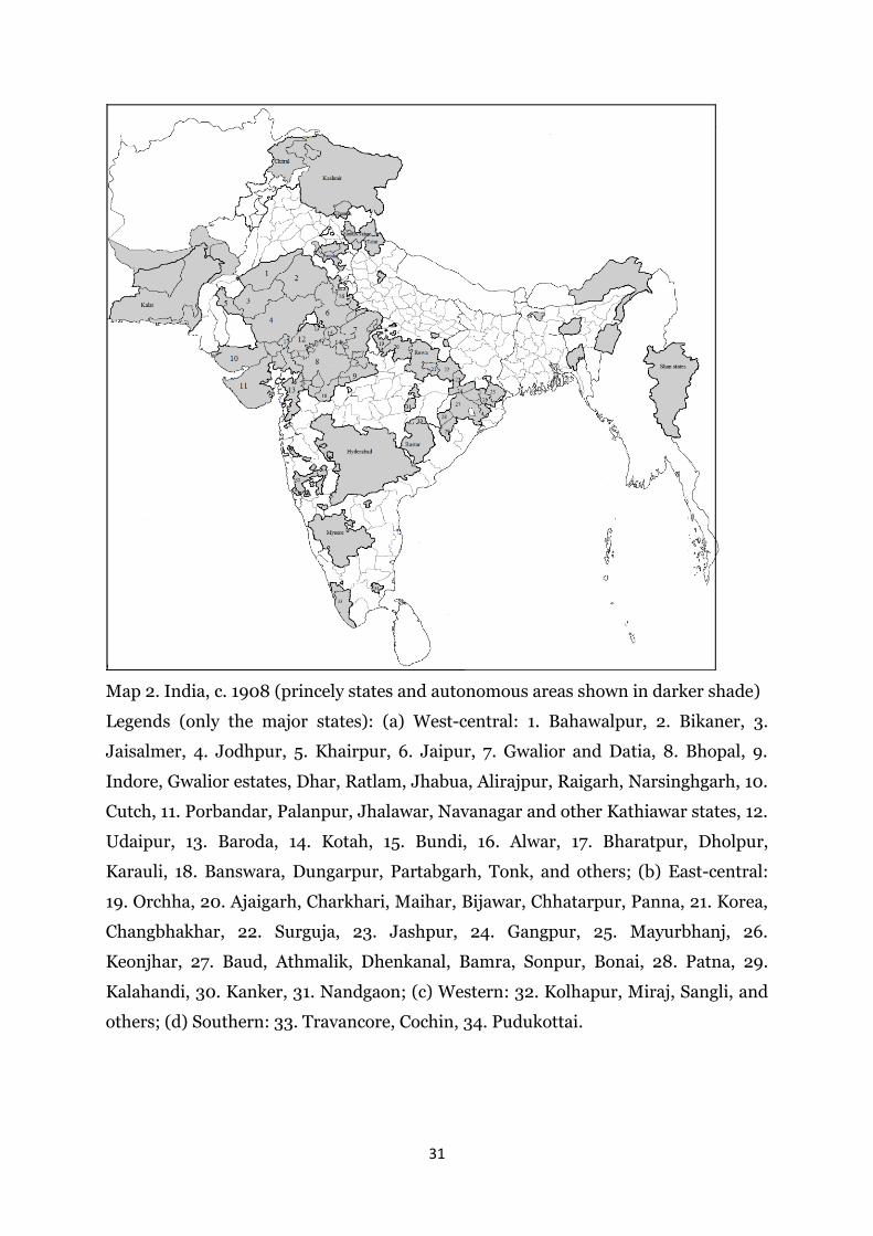
formally the freedom to rule was respected (Map 2).2 The relationship between

British India and the princely states is often captured by the phrase indirect rule.

These princely states were the kingdoms, many of them former vassals of

Maratha or Mughal empires, that British India did not annexe to itself. The political

ground for not doing so was that these states were allies of the British, and those in

northern India had demonstrated the loyalty during the great mutiny (1857). But,

then, nearly all of these states were land-locked, arid or poorly irrigated, with forest

cover, and for these reasons, did not yield as much value as it might cost to acquire

and maintain them. The states left alone were, nevertheless, required to maintain

open borders to commercial traffic. They could have their own currency or legal

systems, but the monetary autonomy existed only in name. Most had little incentive

to insulate themselves from the pan-regional economic tendencies. No state was

known to want to erect obstacles to market integration with British India. Most of

them were also pro-Empire in sentiment and resisted independence in 1947.

Depending partly on when and in what manner colonial rule had come into

existence, the directly ruled territory became differentiated in respect of rural

property rights. Possibly the most important institutional innovation undertaken by

the East India Company state (1793-1820) was the definition of the legal title of

ownership of land and the creation of a system of courts and legal procedures to

verify and uphold the right. This was in theory and in practice a departure from the

past system where land ownership, with or without secure title, was tied to the

performance of fiscal duties, so that a peasant and a tax collector could both lay

claims on a plot of land. The situation had stymied the land market, in the view of the

colonial administrators. Their solution was to create an unencumbered ownership

title. In practice, the title was delivered to former tax collectors (landlords or

zamindars) in one part of India, individual peasants in southern and western India,

and peasant collectives or extended kinship groups in parts of northern India.

Did regional differences in economic conditions derive mainly from

geographical diversity or from political-institutional diversity? Were they mainly

‘natural’ or mainly ‘manmade’? Until recently, the empirical literature did not

present a clear answer to questions like these, which have a bearing on discussions of

2 On general political history of the ‘princely states’, see Fisher (1991); on description of ruling families, Malleson (1875). Current historical scholarship deals mainly with political culture, administrative culture, and social modernization. See, for example, Jeffrey (1978); Bhagavan (2003); and the survey by Zutshi (2009).

6

the long-term growth pattern in India. In the 1960s and the 1970s, a neoclassical

strand in the literature explored the growth-inequality interaction, testing the then

popular hypothesis that market-led growth should benefit regions that had resources

in demand in abundance, whereas a ‘backwash’ effect might lead to a spatial

concentration of the gains from trade (Williamson, 1965; Myrdal, 1957). Another

contemporary strand, inspired by the concepts of ‘enclave’ and ‘parasitical cities’,

paid attention to unequal political power of business groups (Hoselitz, 1954-5; Leys,

1974; Bagchi, 1976). But neither approach engaged with history or geography very

deeply.

A recent scholarship has returned the field to the geography-versus-politics

problem. It tests the association between the political-institutional legacies of

colonialism and late-twentieth-century pattern of regional inequality in the supply of

public goods, and finds it to be statistically significant. One key contribution,

Banerjee and Iyer (2005), make use of the World Bank agriculture and climate

dataset for India, which provides annual averages for 400-odd districts during 1957

to 1986. Their main result, which uses a subset of districts, is that in those districts of

British India where the colonial rulers had delivered property rights to non-

cultivating landlords or zamindars (in 1793), rather than to the cultivating peasant,

agricultural productivity was higher and investments lower in the post-independence

period. The underlying argument is that in the landlord areas, conflicts and lack of

cooperation between the elite and the peasants became more likely and made

lobbying for resources in the post-independence period less successful. Banerjee,

Iyer and Somanathan (2010) use the World Bank dataset for an expanded number of

districts, divide these up into those that were formerly princely states (indirectly

ruled) and those forming part of British India (directly ruled) as well as by landlord

property and peasant property areas. They find that the provision of some of the

public goods examined was negatively correlated with a dummy for districts which

had formerly been directly ruled and under landlord systems.

A third contribution to this scholarship, Iyer (2010), supplements the direct-

indirect-rule data by public goods data for 1961-1991, and estimates the relationship

between being directly ruled in the colonial period and agricultural performance and

provision of public goods in the modern period. In this analysis, the motivation of

princely states to perform is explained with reference to the landed property regimes

and an annexation threat first applied systematically during ‘the doctrine of lapse’ in

7

force between 1846 and 1856. Iyer (2010) finds no significant effect of direct rule on

agriculture, but a negative effect on public goods. The reason adduced for this is that

the princely states were less constrained by British Indian priorities, as well as faced

an incentive to be well-governed, being under threat of removal by the British.3

The confirmation found in this corpus that the princely states were more

progressive than British India and indirect rule more welfare-inducing than direct

rule overturns an earlier result from a more limited statistical test (Hurd, 1975;

Simmons and Satyanarayana, 1979). The new scholarship has spawned several

attempts at extensions (Kapur and Kim, 2006; Chaudhary, 2010) and one critique of

the methodology of Banerjee and Iyer (2005) (Iversen, Palmer-Jones, Sen, 2012).

Although the empirical strategy adopted in these contributions is innovative,

it has limitations. There are three issues in particular. First, the colonialism and

public goods scholarship takes for granted that the formal designation of a region (as

landlord or as a princely state) should in theory correspond to a substantive

institutional type. This issue of the coincidence or otherwise of formal and

substantive institution is under-researched, and where researched, disputed. A few

examples will illustrate the problem. In the core zone of landlordism, Bengal,

historians disagree on who actually controlled land and, in turn, shaped local politics

(Ray, 1979). On the other hand, in some of the princely states, the ‘elite’ who

descended from warlords and nobility much like the landlords in British India

controlled land and influenced the dispensation of public goods. One example of elite

power was Hyderabad, the largest among the princely states (Leonard, 1971). The

public goods literature also assumes that the relationship between British India and

the princely states was significant, uniform, and well-defined. This is questionable

too. One historian, for example, writes, ‘Hyderabad State was technically under

British indirect rule, but this status was one of the least significant things about it’

(Leonard, 2003: 364). It is inevitable that, pending more work on this theme,

historians will identify the formal designation of a region as landlord or a princely

state with a real institutional type. But such practice is at best founded on a shaky

assumption. Therefore, it is also necessary to explore alternative methods that

obviate the need to introduce hard segmentation between regions. I explore one such

alternative, spatial correlation, in this paper.

3 On the conditionality, see Lee-Warner (1910), pp. 280-312.

8

Second, in the public goods scholarship, geography is approximated by an

array of qualities, such as soil, rainfall, and proximity to the coasts, rather than by

any specific concept of zoning. I prefer to follow a classification scheme that derives

from a definite conception of space found in colonial geography. This conception is

justified more fully in the next section.

Third, the design of the tests in the public goods scholarship carries a

potential oversight. The design of the tests involves regressing post-1960 effects on

causes that had been introduced 120-170 years earlier, namely, the formal

inauguration of landlord property in 1793 or an annexation threat that was credibly

applied for the last time in 1848-56. The procedure entails a systematic

underestimation of the role of geographical factors in economic change and regional

differentiation. Geography should matter to economic change in a variety of ways.

Among the most important channels is trade in goods intensive in resources that are

unequally distributed in space. Nineteenth century trade in India was dominated by

agricultural commodity trade under a more or less laisser-faire regime. Therefore,

trade was a geographically influenced process in the nineteenth century. On the other

hand, the collapse of international trade in the 1930s, the severely regulated trade

regime after 1947, prohibition on agricultural trade – all of these factors put an end

to the colonial economic system in which resources and commodities had

contributed more directly to economic growth. Trade-GDP ratio in the 1960s was less

than one-third of what it was in the 1920s. In other words, between 1870 and 1930 a

trade-driven process of growth and regional differentiation had begun and exhausted

itself. Correlation between 1960s variable values with early-1800s variable values

builds in an oversight of this process.

Consider the process that we may miss noticing. Throughout Indian history,

agricultural production, long-distance trade, and the formation of powerful imperial

states were more likely to concentrate in the deltas of eastern and southern India and

the Ganges and Indus floodplains. These areas usually had higher cropping intensity,

greater irrigation potentials, and yielded more revenue per area, than the arid lands,

deserts, forests, and dry uplands in the interior. Major commercial towns tended to

be situated in these areas, reflecting the availability of larger volumes of agricultural

surplus in them. Not only was the quality of land better in the former zones, trade

costs were lower too. The flat terrain and the presence of large rivers made it possible

to move goods and people by the two relatively cheaper modes of long-distance

9

transportation, namely, carts and boats. In the rest of the region, the upland and the

forests made it impossible to move cargo over land by anything other than the

expensive and slow mode of caravan trains.

The British territories contained more of the coasts-deltas-floodplains,

whereas more of the uplands and forests fell within the domain of the princely states

(see Maps 4 and 5). The landlord areas too consisted largely of deltas, coasts, and

riparian plains. This is well recognized in the public goods scholarship (see, for

example, the careful treatment of agriculture in both Banerjee and Iyer, 2005, and

Iyer, 2010). If globalization was indeed a significant influence on regional inequality,

we should expect the British Indian and the landlord areas to forge ahead of the

princely states and non-landlord areas. Even though a key tradable, cotton, came

from the dry-land, the major examples of agricultural commercialization were in fact

located in the floodplains (wheat and sugarcane from Punjab and United Provinces),

the coasts (rice from Krishna-Godavari delta, cotton from coastal Gujarat), and the

deltas (rice from Bengal). Higher land revenue potential led to greater local revenue

available for spending on public goods. Commercial profits were also channelled into

education and health-care on quite an extensive scale, when these profits

concentrated in the port cities, the case of Parsi charitable institutions of Bombay

being a well-known example. The effect is expected to have been reinforced by a bias

in the provision of public goods in favour of those goods that potentially aided

commodity trade. For example, in colonial India, major infrastructure projects were

prioritized with reference to agricultural production (canals) and agricultural trade

(railways). In the mid-nineteenth century documents outlining plans for a railway

system in India, the benefit for trade took precedence. Even as the first twenty-five

years of railway construction proved to be a burden on the exchequer, ‘the trade and

revenues of the country testified to the value of the new means of communication’

(India b, 1908, v. 3: 368).

Putting these pieces together, we should see in the nineteenth century a

virtuous circle develop at the regional level between trade, state capacity, and

infrastructure. We should also see that the collapse of world trade from the 1920s

and the regulated trade regime of post-colonial India put an end to this circle so that

the formerly leading regions fell behind. If this hypothesis has merit, tests of

association between 1960s inequality and institutional causes introduced in 1793 and

1848-56 need to be re-examined for two reasons, (a) they bypass the historical

10

process of economic change and regional differentiation that occurred in between,

and (b) they produce an outcome that is counter-intuitive.

With a contemporary dataset, I revisit the subject.

The data and empirical strategy

The 25-volume Imperial Gazetteer of India (1908) did not set out to collect

statistics. But it made use of a uniform questionnaire in its descriptions of territorial

units, so that it is possible to pick from the descriptive sections numbers pertaining

to area, population, revenue, rainfall, cultivated and irrigated areas, roads, railway

network, literacy, and the size of the largest town. For 430 districts of British India

and 130 princely states, partial or full details are available. The territory includes

lower Burma, as well as the Shan states in eastern Burma over which British India

established overlord status without direct governance or control. Some of the regions

so governed do not yield much usable data. Together, the units for which there is

data (excluding Burma) accounted for 276 million persons and 1.4 million square

miles of territory. According to the census of 1901, India’s population (excluding

Burma) was 284 million, and the area 1.53 million square miles. Despite the

exclusions, then, the Gazetteer dataset still accounts for 97 per cent of population

and 93 per cent of area. Missing data for many of the smaller districts and states

poses a problem. Using nearest comparable units some of the gaps was filled as far as

possible.

In the first step of the statistical analysis, these regional units are classified

into two political clusters (British India and princely states), two institutional

clusters (landlord zones and peasant-property zones), and two geographical clusters

(coasts-deltas-floodplains and deserts-uplands). The first pair is easily defined. One

practical advantage of working with a 1908 dataset is that the political units enter the

analysis exactly as they appear on the map, whereas the use of World Bank data

entails a complicated task of reassigning areas across new boundaries. The Gazetteer

data also allows us to work with undivided India and a much larger set of territorial

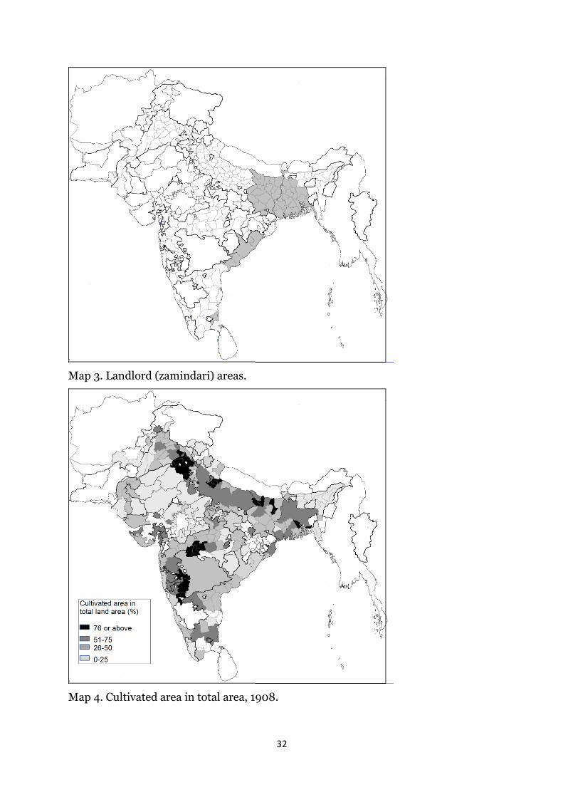
units of both types. The second distinction between landlord property and non-

landlord property has seen a recent controversy over which areas were formally

designated as one or the other (see Iversen, Palmer-Jones, Sen, 2012). I follow the

orthodox classification, where Bengal, Bihar, coastal Orissa, parts of the southeastern

11

coast known as the Circars, and sections in Madras Presidency (especially Ramnad

area) formed units in the zamindari or landlord tenure (see Map 3).

Colonial geography (see, for example, Medlicott, 1862) divided India into four

principal zones, the Himalayas and the submontane, the central and south Indian

plateau, the seaboard and the delta, and the floodplains of the Ganges and the Indus.

I ignore the mountains and the submontane, which were not part of the core

agricultural zone except in narrow fluvial tracts, and consolidate the other zones into

two. By this scheme, a classification consisting of coasts, deltas, and the floodplains

of the Himalayan rivers on the one hand, and the uplands and arid regions in the

interior on the other hand, seems to capture the most crucial difference in resource

conditions well enough.

Productive capacity anywhere in India depended on agricultural conditions.

Agriculture was constrained by the extreme tropical heat and the long dry season,

and helped by replenishment of ground and surface water by the monsoon rains for

three months of the year. In 1908, productivity of land depended only moderately

upon soil nutrients. It depended more directly on cropping intensity, which was a

function of irrigation water. Canals and surface wells, the two common modes of

accessing water bodies depended on the availability of large rivers in proximity as

well as alluvial soil, so that irrigation potentials reinforced the natural productive

capacity of the deltas and the great floodplains. A flat terrain with plentiful rains

allowed for a controllable supply of irrigation water, and therefore, more land

cultivated and above-average cropping intensity (Maps 4 and 5). The deltas,

floodplains, and the coasts satisfied these conditions, or some of them. Uplands and

low-rainfall zones were deficient in irrigation potentials. Because of this reason, the

core agricultural zones in the subcontinent formed in the deltas, the coasts, and the

floodplains of the Indus and the Ganges.

A final point about the procedure adopted here needs an explanation. The

1908 dataset is rich enough to allow us to work with a range of indicators of

economic well-being of regions, including tax collection, literacy, transportation

density, urbanization, and irrigation ratio or the quality of land resources.

Descriptive analysis considers all of these benchmarks. However, none of these

stands for a direct measure of well-being or productive capacity, as income or yield

would. Regional domestic product before 1950 is unavailable. The attempt to

construct regional incomes is somewhat promising for the British Indian provinces

12

(see Caruana-Galizia, 2013, for an innovative reconstruction). But it is a futile quest

for many of the princely states that did not collect basic economic data.

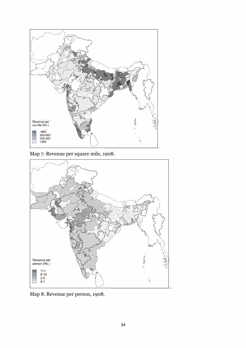
For measurement of inequality, a proxy is used. On the assumption that the

size of the regional government bears a positive relation with the productive capacity

of the territory, the size of the fisc (revenue per square mile) can be used as a proxy of

the productive power of a region. Unlike after independence in 1947, there was little

transfer of saving or revenue between territories, and state revenue came mainly

(over 50 per cent) from land. Production conditions in agriculture depended on

irrigation prospects, which depended on climate and topography.

We do not have much choice in the matter of selecting the benchmark

variable, but the use of revenue per square mile can be defended. Revenue is a

reasonable index of regional productive power if (a) there was a close

interdependence between the fiscal system and the production system, (b) factor

payments mattered little to the composition of regional incomes, and (c) tax rates did

not differ between regions significantly. All three are defensible assumptions.

State revenues were mainly raised from land tax, so that agricultural

production and government finance were closely related. Internal migration did

increase in the colonial period, but with the prevailing low wages and very limited

facilities for remittance, its impact on factor income flows should be relatively small.

In principle, if the tax-rate is high in a low-income area and low in a high-income

one, the same level of collection could hide large inequality in incomes, and

therefore, the use of the proxy could under- or over-estimate inequality. Tax-rates

are not available directly. But the variation in tax-rate is unlikely to have been large.

The rate of taxation on land was based on a tradition of cadastral surveys and

maintenance of local registers that was long-standing and pre-colonial in most parts

of India. The tradition, furthermore, drew on notions of fair taxation that were also

very old. There was an official discourse in British India on the desirability of

following a Ricardian principle of taxing potential scarcity rent, while at the same

time, basing the minimum tax rate upon indigenous tradition. Under these

conditions, the tax rate would have approached, by 1908 at least, when these

principles had been in operation for nearly a century, a uniform level, subject to

13

variations in land quality (see Roy, 2012, for further discussion on land revenue

policy).4

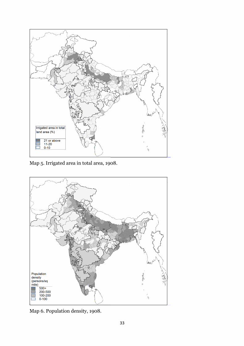
Measures of inequality by this benchmark are sensitive to population in a

systematic way. Any type of region, however defined, that produced more value per

land area measured by fiscal revenue tended to be more densely populated (see Map

6, and contrast Maps 7 and 8). This inverse relationship should suggest that the

higher population density of the well-endowed regions was partly an effect of in-

migration in search of easier agricultural livelihood and partly an effect of lower

mortality rates because these regions ensured food security better. In that case,

population density can be seen as an endogenous variable in a process driven by

unequal resource endowments. This prospect justifies using measures per area rather

than measures per capita.

Using this dataset, I examine the hypotheses that

a. Regions better endowed in natural resources were also better endowed in public

goods, which is tested by a comparison of cluster means;

b. Relative geographical situation exerted a significant impact upon public goods

and productivity, which is tested by estimating spatial correlation; and

c. The extent of regional inequality increased in the free trade era, which is tested by

comparing two revenue datasets fifty years apart.

Comparison of cluster means

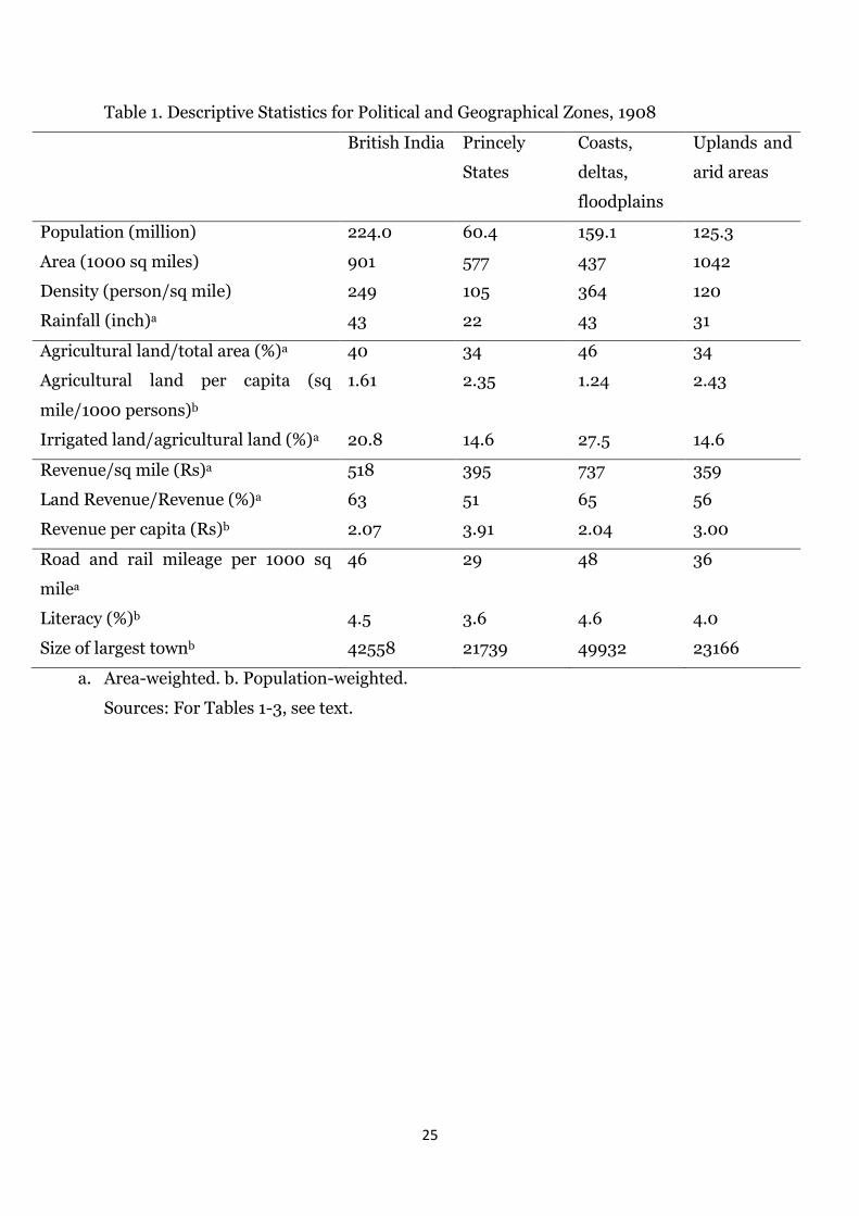
Tables 1 and 2 show the averages of the benchmark indices for these zones.

Table 1 shows that the coastal-deltaic-floodplain regions were on average better-off

than the arid uplands and that the princely states were poorer than British India.

These findings are interdependent since more of the coastal-deltaic-floodplains areas

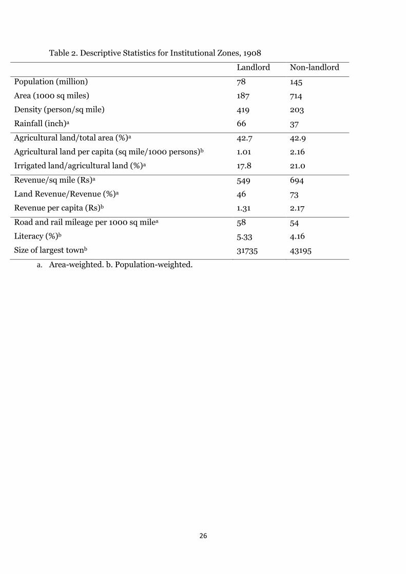
formed part of British India. Table 2 suggests that property regime is not a good

predictor of regional inequality. Some of the indices favour the non-landlord regions,

whereas literacy and transportation density are higher in the landlord regions, if

marginally. Of the public and quasi-public goods on which this dataset has any

4 One potential problem with ignoring tax-rate is that the landlord areas had fixed taxes forever, whereas the non-landlord ones allowed for revisions. In practice, revisions had become rare after 1880. In any case, if tax-rates did differ on this account, it would pose a problem for the use of tax-per-area as a measure of the productivity of the area in question only if the landlord areas appear to yield less tax on average. It would, then, be difficult to identify the effect of tax-rate from the effect of the capacity of the land to produce taxes. In practice, the landlord areas produce more taxes on average at this time, so that this issue can be ignored.

14

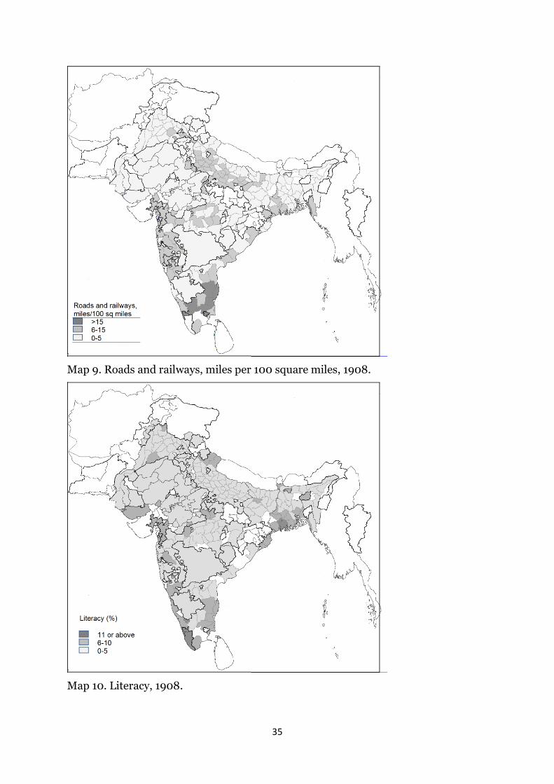
information, transportation density appears to differ widely, being higher in the

delta-coastal-floodplains regions as well as in British India (see also Map 9).

Literacy, however, varies in a narrower range and did not necessarily concentrate in

the endowed zones (see also Map 10). I will return to this finding later. There is also a

difference in level of urbanization (approximated by the size of the largest town)

between geographical and political zones.

A number of results illustrate the poorer endowments of the princely states,

the lower average rainfall, a smaller proportion of cultivable land, lower irrigation

ratio, revenue per square mile, urbanization, transportation density, and literacy

(Table 1, also Maps 1 and 4). Transportation density is especially important because

of its potential link with trade costs. Because of the uplands terrain, all-weather

roads there were very few in the territory of the states. As we have seen, railways

were at the start a private good in British India, and motivated by expected profits

from trade. Not surprisingly, in the floodplains of the Ganges and the Indus, railways

started early (1850s) and followed the major arteries of road and river-borne

commercial traffic. Railways started late in the princely states, and construction was

mainly led by the governments, though in some of the long-distance lines cutting

through the states partnerships with private companies and British Indian

government were also present. If these through lines are excluded, the majority of

the lines constructed by the princely states seem to have served mainly passenger

traffic. In some parts of India (such as Kathiawad in Gujarat), political fragmentation

was so great that the state railways were built in small uncoordinated segments,

often in the outlandish two-feet or ‘narrow’ gauge, that did not feed effectively into

the long distance broad-gauge routes running through British India. This set of

factors accounted for a lower railway density in the states. That being said, the gap in

the railways did narrow over time. From the 1870s, the British Indian government

started taking control of the railway system and non-commercial motivations (such

as famine relief) took precedence. State railway construction gathered speed as well.

What has been said of the roads and the railways, would apply to the ports

with even greater force. The four major ports, Bombay, Calcutta, Madras, and

Karachi, were all located in British India. Among the larger princely states, only

Travancore-Cochin had a long seafront. In turn, the economy of this state was also

more export-oriented than other princely states. Of the other major states, Baroda

15

was well-connected by rail with Bombay port. Still, few of the princely states had easy

access to the sea and a comparable history of long-distance commerce by sea.

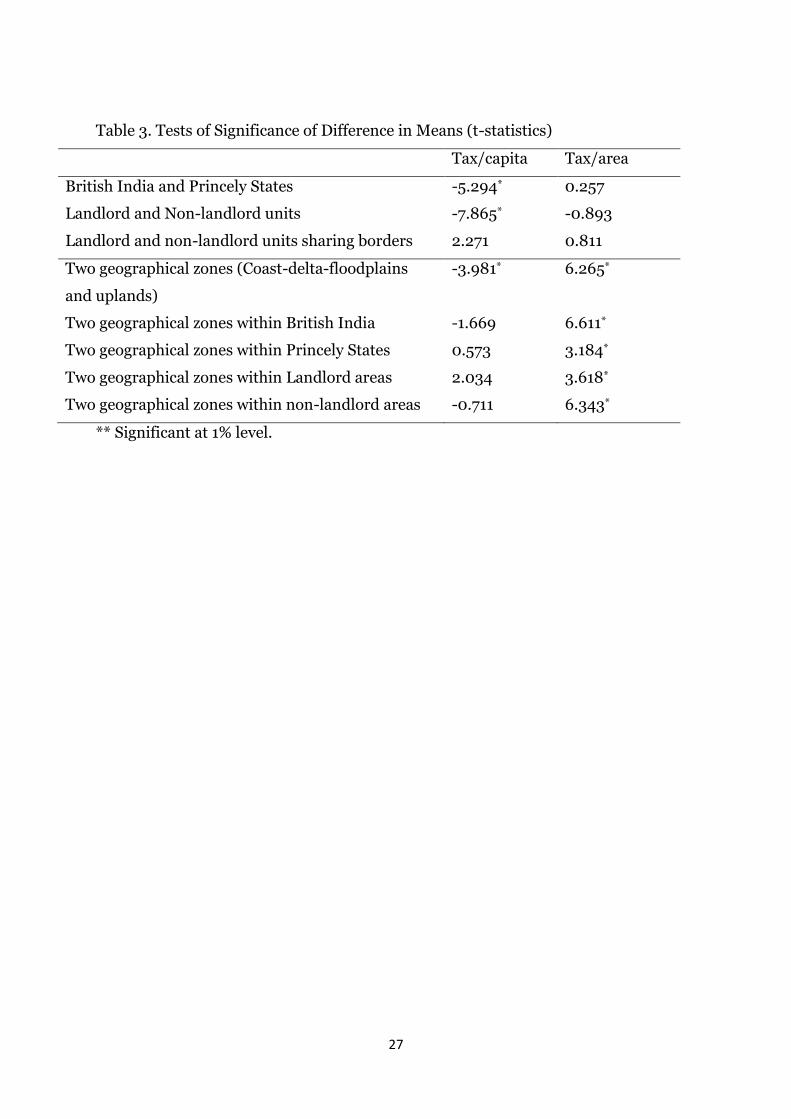
Are the differences between clusters of significant order? Table 3 presents

results of tests of significance of the difference in means. The benchmark variable is

revenue collection. The tests are conducted for pairs of broad clusters, as well as

interactions between them (for example, geographical differences within a political

cluster). In addition, following on a procedure introduced in Banerjee and Iyer

(2005), the difference in means between two reconstructed clusters is conducted,

one of the clusters consisting of landlord territories and the other of non-landlord

territories, subject to the condition that each landlord territory shared a border with

at least one non-landlord territory. This pair is added under the assumption that

contiguous units, even when institutionally different, were geographically similar, so

that if the difference between them turns out to be insignificant the result would

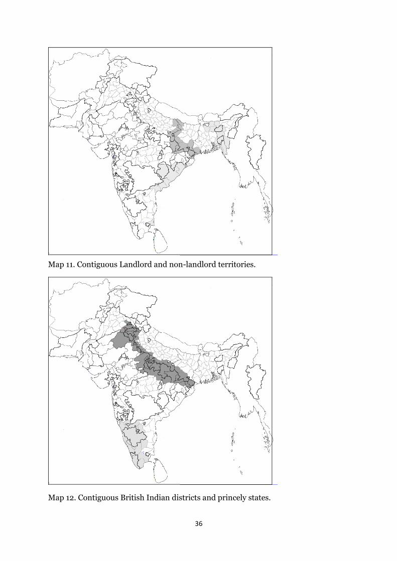
indicate that institutional differences mattered less than we may expect. Map 11

shows the cluster (in darker shade) for which this exercise was done, whereas other

similar clusters of contiguous and institutionally differentiated territories in eastern

and southeastern India (shown in lighter shade) involve too few observations for a

meaningful result.

Table 3 suggests two results. Princely states were significantly better-off than

British India and the non-landlord territorial units significantly better-off than the

landlord ones only if we consider revenue per capita. If, however, we consider

revenue per square mile, differences between political and institutional clusters cease

to be significant, and geographical differences alone matter (see also Maps 8 and 9).

In the case of contiguous units, the nature of landed property makes little difference

to either one of the benchmarks.

In view of the criticism of cluster-based analyses offered earlier, it is desirable

that we confirm the nature of the differentiation by means that do not depend on

clustering at all. Spatial autocorrelation supplied such a tool.

Spatial autocorrelation

Autocorrelation in cross-section datasets is a recognized problem, but tends to

receive less attention in economic history than that in time-series or pooled data.

This is so because the phenomenon of correlated errors is more pro-intuitive in

temporal data as the effect of ‘inertia’ than correlated errors in spatial data. In recent

16

years, spatial autocorrelation has been used more often in several fields straddling

economics and geography. One example is consumption studies, when the

consumption of one family depends on the consumption by its next-door neighbour.

A regression of consumption on income or wealth will not produce efficient estimates

in such contexts and a special test is needed to measure the extent of correlation

between neighbour units (Case, 1999). Other examples of the use of the tool are

studies on diffusion of technological innovation (Ó Huallacháin and Leslie, 2005),

the clustering of urban poverty (Longley and Tobón, 2004), and the spread of

epidemic contagion (Smallman-Raynor, Johnson and Cliff, 2002).

The technique finds frequent use in geography. This is to be expected, for the

effect of such qualities of the earth as soil, rainfall or terrain does not change

drastically, but only gradually, between one spatial unit and another contiguous

spatial unit. Therefore, it is standard in spatial econometrics to assume that the

features of one unit should predict features of neighbourhood units, giving rise to

autocorrelation between the errors. As in the case of time-series data the smaller the

unit the bigger is the correlation. Conversely, if in a spatial economic dataset such as

the one in question autocorrelation turns out to be significant, that characteristic can

be read as geographical in origin. In theory, merely the presence of a high

autocorrelation is not sufficient proof that geography is more important than other

influences, because we do not know why neighbourhood exerts an influence. Such

patterns can follow, for example, if administrative practices are transferable between

contiguous areas. But, then, any effect that crosses borders between territorial units

does not necessarily influence the aggregate measure. If such local effects are a mix

of positive and negative correlation (an example of a negative effect being one where

one unit draws trade away from or exploits a neighbour), they can even cancel each

other out. The coefficient will be significant if a large number of units display

dependence on neighbours, which points at a single process generating such effect. If

we are explaining the generation of land revenue, distribution of agricultural

resources is the likely reason. If the cluster averages also point in the same direction,

there is stronger confirmation of the hypothesis.

Regression models, in the presence of such a process, can be of questionable

value. If we have reason to assume that the causal model is such that the error of one

unit should predict errors of neighbourhood units, it is necessary to measure the

17

extent of the problem. A regression with fixed effects such as region dummy will still

entail an underestimation of the residual variance common to all such cases.

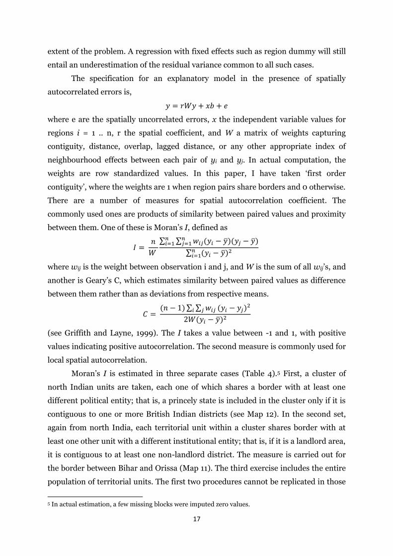
The specification for an explanatory model in the presence of spatially

autocorrelated errors is,

where e are the spatially uncorrelated errors, x the independent variable values for

regions i = 1 .. n, r the spatial coefficient, and W a matrix of weights capturing

contiguity, distance, overlap, lagged distance, or any other appropriate index of

neighbourhood effects between each pair of yi and yj. In actual computation, the

weights are row standardized values. In this paper, I have taken ‘first order

contiguity’, where the weights are 1 when region pairs share borders and 0 otherwise.

There are a number of measures for spatial autocorrelation coefficient. The

commonly used ones are products of similarity between paired values and proximity

between them. One of these is Moran’s I, defined as

∑ ∑

∑

where wij is the weight between observation i and j, and W is the sum of all wij’s, and

another is Geary’s C, which estimates similarity between paired values as difference

between them rather than as deviations from respective means.

∑ ∑

(see Griffith and Layne, 1999). The I takes a value between -1 and 1, with positive

values indicating positive autocorrelation. The second measure is commonly used for

local spatial autocorrelation.

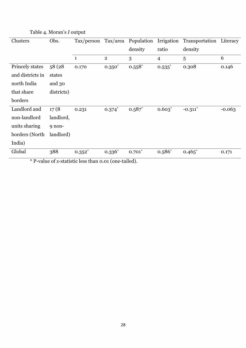
Moran’s I is estimated in three separate cases (Table 4).5 First, a cluster of

north Indian units are taken, each one of which shares a border with at least one

different political entity; that is, a princely state is included in the cluster only if it is

contiguous to one or more British Indian districts (see Map 12). In the second set,

again from north India, each territorial unit within a cluster shares border with at

least one other unit with a different institutional entity; that is, if it is a landlord area,

it is contiguous to at least one non-landlord district. The measure is carried out for

the border between Bihar and Orissa (Map 11). The third exercise includes the entire

population of territorial units. The first two procedures cannot be replicated in those

5 In actual estimation, a few missing blocks were imputed zero values.

18

regions where a reasonable number of contiguous units with opposing political-

institutional configuration cannot be found, or where these entities are too dissimilar

in size. For example, the first procedure can be repeated only for a much smaller

number of states and districts in south India. Similarly, the second procedure can be

in principle carried out for eastern Bengal along the borders of Assam (non-landlord)

and Bengal (landlord), but the number of observations would be too few (the clusters

excluded are shown in lighter shade in Maps 11 and 12).

If the null hypothesis is that geographical situation exerts no systematic

influence on the economic profile of regions, we would expect the autocorrelation

coefficient to take a value near zero. Such a value might signify that political status or

institutional features exert a strong influence in the dataset.6 If the coefficient takes a

significant value, we should conclude that, overriding political-cum-institutional

differences, neighbouring units tend to be sufficiently similar.

Table 4 shows the results of the exercise. Revenue per area, population

density, revenue per person and irrigation ratio all show positive autocorrelation; in

ten of the twelve estimates the coefficient is significant. When we come to public and

quasi-public goods, such as roads and schools, the neighbourhood effect seems to

weaken, even though it remains positive in the case of states and districts, and in the

global dataset. The exceptional case of literacy is pro-intuitive, and shows that only in

education, where ideology of social welfare played an explicit role, was there an

effective catching up via state intervention. Overall, it seems reasonable to conclude a

strong effect of geographical situation, qualified but not overturned in the case of

public goods.

The final step in the analysis consists of asking, was there divergence or

convergence in colonial India? In order to answer the question, I combine the 1908

dataset with an earlier source.

Trend

The earlier source in question (Anon., 1853, Thornton, 1853) had collected

data on the size of major states and East India Company territories. The source

covers 13 regional political units, including major princely states. Although data for 6 There is an additional reason to exclude these zones from the test. The coefficient cannot be easily interpreted if geographical features change drastically over relatively short distances. This problem is likely to affect the outcome for the southern peninsula, which is a mix between arid uplands and fertile river valleys, and for eastern Bengal where a cordillera of the Himalayas run more or less along the border between landlord and non-landlord zones. These areas are excluded from the test.

19

the British Indian territories began to be presented regularly and in reasonable detail

from about 1840, this was the first time, and the only occasion in the nineteenth

century when the states and the provinces received equal coverage in the same

source. The data consists of area, population and revenue.

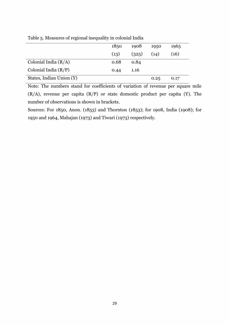
Again using only revenue collection data, I estimate coefficients of variation

(the measure known as unconditional σ-convergence). It has limitations, but it is

easy to use and a better measure to use when the number of observations is small, as

in the case of 1853. Subject to the caution that the 1850 finding cannot be very

robust, the results (Table 5) point at increasing inequality in the second half of the

nineteenth century. For a shorter span of time within the range, 1875-1911, Caruana-

Galizia (2013) finds evidence of convergence in regional GDP. The units are the

British Indian provinces. For what the 1850 data are worth, the Gazetteer dataset

suggests an unchanging level of inequality among the British Indian territories, and a

divergence only if we include the states.

On the other hand, there was almost certainly a great decline in inequality in

the twentieth century, which trend continued on in the early decades of planned

development under a national government. Again, these trends alert us to the

problem that the results are sensitive to whether we normalize the variables with

area or population. Between 1853 and 1908, population was stagnant, but population

growth accelerated after 1920, mainly in the fertile plains. By 1960, then, the gains of

the more resource-endowed regions were being shared amongst a much larger

population than in the colonial times.

Conclusion

The statistical analysis carried out above leads to the conclusion that the effect

of geographical endowments on the pattern of regional inequality in fiscal capacity

and public goods was significant in the late nineteenth century. The conclusion is

based on three specific findings derived from a 1908 dataset: averages differed

between geographical zones more consistently than between political and

institutional zones, neighbourhood exerted a positive and significant effect on

regional attributes, and regional inequality rose when there was free trade and fell

when free trade ended.

The conclusion differs from that of the recent scholarship on colonialism and

public goods discussed earlier, which discounts the influence of geographical

20

differences upon regional inequality (Banerjee and Iyer, 2005; Banerjee, Iyer and

Somanathan, 2011; Iyer, 2012). There are several possible reasons for a discrepancy.

First, subject to the limitations of the 1908 dataset, the present paper makes use of a

specific unit of measurement, namely, fiscal capacity per area. Second, the present

paper classifies geographical zones differently, following a contemporary

classification scheme. Third, resource endowments did, in fact, play a bigger role in

the process of economic change at the turn of the twentieth century. Around that

time it outweighed other influences; but the effect faded away by the middle of the

twentieth century.

The third possibility, a plausible case for which is made in the paper, suggests

a particular dynamic of economic transformation in prewar India, led relatively more

by globalization and market integration, rather than by the region’s own specific

political heritage. About 1908, the deltas and the floodplains allowed for greater

density of cultivation than the rest of India, and therefore, more revenue per land. A

virtuous circle developed between land productivity, state capacity, and

transportation density. The circle worked better with roads than railway, where the

gap narrowed, partly because railways began as a private good in British India and

was state-led in the princely states all along. A similar qualification needs to be added

with literacy. Again, much schooling in British India was a private good and sensitive

to commercialization, whereas in the princely states, education and health-care were

supplied by the government to a greater extent.

The final piece in the story is the hypothesis of a rise and decline of regional

inequality. By virtue of possession of more fertile land, the deltas, floodplains, and

coasts were better situated to gain from the nineteenth century globalization, which

encouraged export of crops like wheat and rice, increased the capacity of the states as

well as commercial actors, and led to more spending both on private and government

accounts on roads, railways, schools, and hospitals. The geographically endowed

zones took part in a ‘Smithian’ growth process, whereas the princely states were less

able to do so.7 The Smithian process slowed after the Great Depression, and was

deliberately weakened after 1947. After 1931, the colonial state became bankrupt, the

world market in primary products crashed, the ideology of laisser-faire was under

attack, a new ideology of the developmental state was in ascendance, and growing

7 This is economic growth driven by the extension of markets with or without institutional and technological change. For a discussion, see Saito (2006).

21

fear of famine led to the imposition of strict controls over commodity trade. When

social overhead expenditure was made a priority by the rising ideological tide, the

princely states proved less constrained by the commitment to imperial priorities than

was British India, whereas the commodity processing and exporting zones lost their

lead in the new economy.

References

ACEMOGLU, D., SIMON JOHNSON AND JAMES A. ROBINSON (2001). ‘The

Colonial Origins of Comparative Development: An Empirical Investigation‘,

American Economic Review 91, 1369-1401.

ANON. (1853). The Native States of India (Pamphlet), London.

AUSTIN, G. (2008). ‘The ‘Reversal of Fortune’ Thesis and the Compression of

History: Perspectives from African and Comparative Economic History’, Journal of

International Development 20, 996-1027.

BAGCHI, A.K. (1976). ‘Reflections on Patterns of Regional Growth in India under the

British Rule’, Bengal Past and Present 95, 247-89.

BANERJEE, A. AND L. IYER (2005). ‘History, Institutions, and Economic

Performance: The Legacy of Colonial Land Tenure Systems in India’, American

Economic Review 95, 1190-1213.

BANERJEE, A., L. IYER, R. SOMANATHAN (2011). ‘History, Social Divisions and

Public Goods in Rural India’, Journal of the European Economic Association 3, 39-

47.

BAYLY, C.A. (1985). ‘State and Economy in India over Seven Hundred Years’,

Economic History Review 38, 583-96.

BHAGAVAN, M. (2003) Sovereign Spheres: Princes, Education and Empire and

Colonial India. Delhi: Oxford University Press.

CARUANA-GALIZIA, P. (2013). ‘Indian Regional Income Inequality: Estimates of

Provincial GDP, 1875-1911’, Economic History of Developing Regions, 28, 1-27.

CASE, A.C. (1991). ‘Spatial Patterns in Household Demand’, Econometrica, 59, 953-

965.

CHAUDHARY, L. (2010) ‘Land Revenues, Schools and Literacy: A Historical

Examination of Public and Private Funding of Education’, Indian Economic and

Social History Review 47, 179-204.

22

COPLAND, I. (1997) The Princes of India in the Endgame of Empire 1917-1947.

Cambridge: Cambridge University Press.

FISHER, M. (1991) Indirect Rule in India: Residents and the Residency System,

1764-1858, Delhi and New York: Oxford University Press.

GRIFFITH, D. AND L. LAYNE. (1999). A Casebook for Spatial Statistical Data

Analysis, New York: Oxford University Press.

HOSELITZ, B.F. (1954-5) ‘Generative and Parasitic Cities’, Economic Development

and Cultural Change 3, pp. 278-94.

HURD, J. (1975), ‘The Economic Consequences of Indirect Rule in India’, Indian

Economic and Social History Review 12, 169-80.

INDIA (1908). The Imperial Gazetteer of India, vols. 1-31, Oxford: Oxford University

Press.

IVERSEN, V., R. PALMER-JONES, AND K. SEN (2012). ‘On the Colonial Origins of

Agricultural Development in India: A Re-examination of Banerjee and Iyer, ‘History,

Institutions and Economic Performance’’, University of Manchester Brooks World

Poverty Institute Working Paper No. 174.

IYER, L. (2010). ‘Direct versus Indirect Colonial Rule in India: Long-term

Consequences’, Review of Economics and Statistics 92, 693-712.

JEFFREY, R., ed. (1978). People, Princes and Paramount Power. Society and

Politics in the Indian Princely States, Delhi: Oxford University Press.

KAPUR, S. AND S. KIM (2006). ‘British Colonial Institutions and Economic

Development in India’, NBER Working Paper No. 12613, Cambridge, Mass.

LA PORTA, R., F. LOPEZ-DE-SILANES, AND A. SHLEIFER (2008). ‘The Economic

Consequences of Legal Origins’, Journal of Economic Literature 46, 285–332.

LANDES, D. (1998). The Wealth and Poverty of Nations: Why Some Are So Rich

and Some So Poor, New York: Harvard University Press.

LEE-WARNER, W. (1910). The Native States of India, London: Macmillan.

LEONARD, K. (1979), ‘The Hyderabad Political System and its Participants’, Journal

of Asian Studies, 30, 569-82.

LEONARD, K. (2003). ‘Reassessing Indirect Rule in Hyderabad: Rule, Ruler, or

Sons-in-Law of the State?’, Modern Asian Studies, 37, 363-79.

LEYS, C. (1974). Underdevelopment in Kenya: The Political Economy of Neo-

colonialism 1964-71, Berkeley and Los Angeles: University of California Press.

23

LONGLEY, P.A. and C. TOBÓN (2004). ‘Spatial Dependence and Heterogeneity in

Patterns of Hardship: An Intra-Urban Analysis’, Annals of the Association of

American Geographers, 94, 503-519.

MAHAJAN, O.P. (1973). ‘Regional Economic Development in India 1950-51 to 1965-

66’, PhD dissertation, Kurukshetra University.

MALLESON, G.B. (1875). An Historical Sketch of the Native States of India,

London: Longmans, Green.

MEDLICOTT, J.G. (1862). Cotton Hand-Book for Bengal, Calcutta: Government of

Bengal.

MYRDAL, G. (1957). Economic Theory and Underdeveloped Regions, London:

Duckworth.

Ó HUALLACHÁIN, B. and T.F. LESLIE (2005). ‘Spatial Convergence and Spillovers

in American Invention’, Annals of the Association of American Geographers, 95,

866-86.

RAY, R. (1979). Change in Bengal Agrarian Society c1760-1850, Delhi: Manohar.

ROY, T. (2012), The Economic History of India 1857-1947, Delhi: Oxford University

Press.

SACHS, J. (2003). ‘Institutions Don’t Rule: Direct Effects of Geography on Per

Capita Income’, NBER Working Paper No. 9490, Cambridge, Mass..

SAITO, O. (2006). ‘Money, Credit and Smithian Growth in Tokugawa Japan’,

Institute of Economic Research Discussion Paper, Hitotsubashi University, Tokyo.

SIMMONS, C. AND B.R. SATYANARAYANA (1979). ‘The Economic Consequences of

Indirect Rule in India: A Re-appraisal’, Indian Economic and Social History Review

16, 185-206.

SMALLMAN-RAYNOR, M., N. JOHNSON AND A.D. CLIFF (2002). ‘The Spatial

Anatomy of an Epidemic: Influenza in London and the County Boroughs of England

and Wales, 1918-1919’, Transactions of the Institute of British Geographers, 27,

452-470.

SOKOLOFF, K.L. AND S.L. ENGERMAN (2000). ‘History Lessons: Institutions,

Factors Endowments, and Paths of Development in the New World’, Journal of

Economic Perspectives 14, 217-232.

THORNTON, E. (1853). Statistical Papers relating to India, London: East India

Company.

24

TIWARI, S.G. (1971). ‘Regional Accounting in India’, Review of Income and Wealth

17, 103-117.

WASHBROOK, D. (2001). ‘Eighteenth Century Issues in South Asia’, Journal of the

Economic and Social History of the Orient 44, 372-83.

Williamson, J.G. ‘Regional Inequality and the Process of National Development: A

Description of the Patterns’, Economic Development and Cultural Change 13, No. 4

(1965): 3-84.

Williamson, J.G. Trade and Poverty: When the Third World Fell Behind, Cambridge

Mass.: MIT Press, 2010.

Zutshi, C. ‘Re-visioning Princely States in South Asian Historiography: A Review’,

Indian Economic and Social History Review 46, No. 3 (2009): 301-13.

25

Table 1. Descriptive Statistics for Political and Geographical Zones, 1908

British India Princely

States

Coasts,

deltas,

floodplains

Uplands and

arid areas

Population (million) 224.0 60.4 159.1 125.3

Area (1000 sq miles) 901 577 437 1042

Density (person/sq mile) 249 105 364 120

Rainfall (inch)a 43 22 43 31

Agricultural land/total area (%)a 40 34 46 34

Agricultural land per capita (sq

mile/1000 persons)b

1.61 2.35 1.24 2.43

Irrigated land/agricultural land (%)a 20.8 14.6 27.5 14.6

Revenue/sq mile (Rs)a 518 395 737 359

Land Revenue/Revenue (%)a 63 51 65 56

Revenue per capita (Rs)b 2.07 3.91 2.04 3.00

Road and rail mileage per 1000 sq

milea

46 29 48 36

Literacy (%)b 4.5 3.6 4.6 4.0

Size of largest townb 42558 21739 49932 23166

a. Area-weighted. b. Population-weighted.

Sources: For Tables 1-3, see text.

26

Table 2. Descriptive Statistics for Institutional Zones, 1908

Landlord Non-landlord

Population (million) 78 145

Area (1000 sq miles) 187 714

Density (person/sq mile) 419 203

Rainfall (inch)a 66 37

Agricultural land/total area (%)a 42.7 42.9

Agricultural land per capita (sq mile/1000 persons)b 1.01 2.16

Irrigated land/agricultural land (%)a 17.8 21.0

Revenue/sq mile (Rs)a 549 694

Land Revenue/Revenue (%)a 46 73

Revenue per capita (Rs)b 1.31 2.17

Road and rail mileage per 1000 sq milea 58 54

Literacy (%)b 5.33 4.16

Size of largest townb 31735 43195

a. Area-weighted. b. Population-weighted.

27

Table 3. Tests of Significance of Difference in Means (t-statistics)

Tax/capita Tax/area

British India and Princely States -5.294* 0.257

Landlord and Non-landlord units -7.865* -0.893

Landlord and non-landlord units sharing borders 2.271 0.811

Two geographical zones (Coast-delta-floodplains

and uplands)

-3.981* 6.265*

Two geographical zones within British India -1.669 6.611*

Two geographical zones within Princely States 0.573 3.184*

Two geographical zones within Landlord areas 2.034 3.618*

Two geographical zones within non-landlord areas -0.711 6.343*

** Significant at 1% level.

28

Table 4. Moran’s I output

Clusters Obs. Tax/person Tax/area Population

density

Irrigation

ratio

Transportation

density

Literacy

1 2 3 4 5 6

Princely states

and districts in

north India

that share

borders

58 (28

states

and 30

districts)

0.170 0.350* 0.558* 0.535* 0.308 0.146

Landlord and

non-landlord

units sharing

borders (North

India)

17 (8

landlord,

9 non-

landlord)

0.231 0.374* 0.587* 0.603* -0.311* -0.063

Global 388 0.352* 0.336* 0.701* 0.586* 0.465* 0.171

* P-value of z-statistic less than 0.01 (one-tailed).

29

Table 5. Measures of regional inequality in colonial India

1850

(13)

1908

(325)

1950

(14)

1965

(16)

Colonial India (R/A) 0.68 0.84

Colonial India (R/P) 0.44 1.16

States, Indian Union (Y) 0.25 0.17

Note: The numbers stand for coefficients of variation of revenue per square mile

(R/A), revenue per capita (R/P) or state domestic product per capita (Y). The

number of observations is shown in brackets.

Sources: For 1850, Anon. (1853) and Thornton (1853); for 1908, India (1908); for

1950 and 1964, Mahajan (1973) and Tiwari (1973) respectively.

30

Map 1. Rainfall and topography, 1908

31

Map 2. India, c. 1908 (princely states and autonomous areas shown in darker shade)

Legends (only the major states): (a) West-central: 1. Bahawalpur, 2. Bikaner, 3.

Jaisalmer, 4. Jodhpur, 5. Khairpur, 6. Jaipur, 7. Gwalior and Datia, 8. Bhopal, 9.

Indore, Gwalior estates, Dhar, Ratlam, Jhabua, Alirajpur, Raigarh, Narsinghgarh, 10.

Cutch, 11. Porbandar, Palanpur, Jhalawar, Navanagar and other Kathiawar states, 12.

Udaipur, 13. Baroda, 14. Kotah, 15. Bundi, 16. Alwar, 17. Bharatpur, Dholpur,

Karauli, 18. Banswara, Dungarpur, Partabgarh, Tonk, and others; (b) East-central:

19. Orchha, 20. Ajaigarh, Charkhari, Maihar, Bijawar, Chhatarpur, Panna, 21. Korea,

Changbhakhar, 22. Surguja, 23. Jashpur, 24. Gangpur, 25. Mayurbhanj, 26.

Keonjhar, 27. Baud, Athmalik, Dhenkanal, Bamra, Sonpur, Bonai, 28. Patna, 29.

Kalahandi, 30. Kanker, 31. Nandgaon; (c) Western: 32. Kolhapur, Miraj, Sangli, and

others; (d) Southern: 33. Travancore, Cochin, 34. Pudukottai.

32

Map 3. Landlord (zamindari) areas.

Map 4. Cultivated area in total area, 1908.

33

Map 5. Irrigated area in total area, 1908.

Map 6. Population density, 1908.

34

Map 7. Revenue per square mile, 1908.

Map 8. Revenue per person, 1908.

35

Map 9. Roads and railways, miles per 100 square miles, 1908.

Map 10. Literacy, 1908.

36

Map 11. Contiguous Landlord and non-landlord territories.

Map 12. Contiguous British Indian districts and princely states.