Geographical. Reports

VALUATION OF GOODS TRANSPORTATION CHARACTERISTICS

- A Study of a Sparsely Populated Area

Kerstin Westin

Department of Geography Umeå university, Sweden No 12

VALUATION OF GOODS

TRANSPORTATION CHARACTERISTICS

- A Study of a Sparsely Populated Area.

Akademisk avhandling som med vederbörligt tillstånd

av rektorsämbetet vid Umeå universitet för vinnande av filosofìe doktorsexamen

framlägges till offentlig granskning vid geografiska institutionen,

Umeå universitet fredagen den 3 juni 1994, kl 13.15

sal B2, Södra paviljongerna

av Kerstin Westin

fil. kand.

VALUATION OF GOODS TRANSPORTATION CHARACTERISTICS - A S tudy of A S parsely Populated Area

Kerstin Westin, Department of Geography, Umeå University, Sweden

Abstract: This study describes how consumers and providers of transportation services in a sparsely populated area valuate different transportation characteristics and estimates how these valuations might affect the total goods flows and the flows on individual Origin-Destination links. It also tests Stated-Preference methods as a tool for valuating transportation characteristics.

The hypothesis was that transportation consumers in sparsely populated areas are more sensitive to changes in the transportation characteristics cost and frequency than they are to changes in goods safety, time accuracy, and delivery time. The reason for this assumption was that the supply of transport modes and transport operators in these areas is limited in comparison to more urban areas. Acceptable transportation costs, in the sense that transportation is economically feasible, and possibilities to obtain a certain minimum transportation frequency are essential. It might, therefore, be necessary to renounce demands for time accuracy, goods safety, and delivery time.

The results indicate that the consumers were most sensitive tp lowered distribution frequency. The probability of accepting a transportation service dropped by .19 when frequency decreased from three times to once per week. Changes in the characteristics delivery time and time accuracy were also significant. Reduced frequency would, from a consumer perspective, also result in the largest impact on the total goods. However, a cost increase of 25 percent and lower goods safety would result in a greater reduction of the total goods flow than would longer delivery time and lower time accuracy.

The providers, on the other hand, were very sensitive to increased costs and lower revenues. A drop in quantity from 90 percent to 40 percent vehicle utilization was also significant. However, respondents in the strata 'private trucks' assigned more importance to changes in frequency and quantity. The largest effect on the total goods flow would be caused by a 25 percent cost increase. High demands on time accuracy would affect the goods flow more than would lowered revenue.

A significant conclusion is that the Stated-Preference method used is an adequate tool in valuating transportation characteristics. However, great care must be taken in formulating the characteristics and levels used. Also, in addition to the characteristics tested in this study, there may be other characteristics that help explain the probability that consumers and providers in sparsely populated areas will accept a transport

Keywords: Just-In-Time. Goods transportation. Sparsely populated areas.

Geographical reports No 12. Department of Geography. Umeå university, Sweden. ISBN 91-7174-909-8 ISSN 0349-4683

Geographical Reports no 12

Valuation of Goods Transportation Characteristics

- A Study of a Sparsely Populated Area

Kerstin Westin

Published by The Department of Geography

Umeå university Sweden

UMEÅ 1994

Kerstin Westin

Valuation of Goods Transportation Characteristics - A Study of a Sparsely Populated Area

ISBN 91-7174-909-8 ISSN 0349-4683

Department of Geography Umeå university S-901 87 UMEA Sweden

TRYCKERIET i Robertsfors 1994

CONTENTS

1. INTRODUCTION 1

2 CHANGE IN GOODS TRANSPORT 4 2.1 Development of goods transport 4 2.1.1 Business logistics 4 2.1.2 Business logistics and sparsely populated areas 8 2.2 Aims and method 9 2.3 Geographical area of the study 11 2.4 Outline of the study 14

3 THEORETICAL FRAMEWORK 15 3.1 Transportation and geography 15 3.1.1 Transportation as a topic 15 3.1.2 Transportation and economic development 18 3.2 Spatial aspects of transportation 23 3.2.1 Transportation costs 25 3.2.2 Criticism of the spatial emphasis 27 3.3 Behavioural aspects on transportation 29 3.4 Business logistics 33 3.4.1 Definition of concepts 34 3.4.2 Development of business logistics 37 3.4.3 Characteristics of transportation services 39

4 GOODS TRANSPORT IN SWEDEN 42 4.1 General description 42 4.1.1 Short-distance transport 45 4.1.2 Long-distance transport 46 4.1.3 Forecast 47 4.2 Regional differences 49 4.3 Transportation authorities and providers 55 4.3.1 Road transport 55 4.3.2 Rail transport 58 4.3.3 Sea transport 60 4.4 Swedish transport policy 61

5 GOODS TRANSPORTATION IN A SPARSELY POPULATED AREA • THE EXAMPLE OF SOUTHERN LAPPLAND 62

5.1 General geographic description 62 5.2 Network 65 5.3 Actors 66 5.3.1 Transportation consumers 66 5.3.2 Transportation providers 67 5.4 Goods flows 70 5.4.1 Distribution by transport modes 70 5.4.2 Distribution by goods commodities 70 5.4.3 Distribution by routes 71

6 PERCEPTION OF TRANSPORTATION CHARACTERISTICS 74

6.1 Method 74 6.1.1 Stated-Preference methods 74 6.1.2 Choice of characteristics and levels 77 6.1.3 Experimental design 80 6.1.4 Survey 81 6.2 Results 85 6.2.1 Transportation consumers 85 6.2.2 Transportation providers 90 6.2.3 Performance of the regression models 96 6.3 Changes in the transportation market 96 6.3.1 Transportation consumers 97 6.3.2 Transportation providers 98 6.4 SP-methods as a method 100

7 SUMMARY AND CONCLUSIONS 102

APPENDIXES: A. Counties and provincial capitals of Sweden 107 B. Experimental design using a fractional factorial design 109 C. SP-questionnaire for transportation consumers 111 D. SP-questionnaire for transportation providers 113

REFERENCES 117

LIST OF TABLES

Table 2.1 The total cost of logistic activities (TCL), Gross Domestic Product (GDP), and the relation TCL/GDP, 1970-1986.(1970 prices.)

Table 2.2 Logistics cost in million SEK per activity, 1979-1986.(1970 prices.)

Table 2.3 Population, area, and population density in the municipalities of Southern Lappland, the county of Västerbotten, and in Sweden in average, in January 1991.

Table 4.1 Distribution of domestic goods by transport mode in the period 1970-1990 in million tons and market share.

Table 4.2 Goods transport performance in Sweden between 1960 and 1990 in billion ton kilometers.

Table 4.3 Distribution of transported goods by trade in 1980. Table 4.4 Road status and state expenditure for maintenance

and construction in 1991. Table 4.5 Transport characteristics for trucks for hire and

private trucks in 1990. Table 5.1 Distribution (in percent) of population according

to age, employment in different sectors, and employment rate in Southern Lappland, and Sweden in 1991.

Table 5.2 Employment in different trades (distribution in percent) in Southern Lappland, and Sweden in 1991.

Table 5.3 Transported goods and distribution of goods by Origin-Destination and transport mode in Västerbotten and Sweden in 1980.

Table 5.4 Distribution of total truck goods by commodity in Southern Lappland in 1987.

Table 5.5 Distribution of assembled cargo by Origin-Destination in Southern Lappland in 1987.

Table 6.1 Characteristics and levels in the experiments for transportation consumers.

Table 6.2 Characteristics and levels in the experiments for transportation providers.

Table 6.3 Sample size and response rate. Table 6.4 Mean values of transportation consumer's perception of

transportation characteristics in Southern Lappland in 1991 Table 6.5 Mean values of transportation consum er's probability

of accepting transportation services in Southern Lappland in 1991.

13

42

43

45 57

58

63

67

68

71

72

78

80

83 87

88

Table 6.6 Estimates of coefficients in the regression model for 90 transportation consumer's probability of accepting a transportation service in Southern Lappland on 1991.

Table 6.7 Mean values of transportation provider's perception 91 of transportation characteristics in Southern Lappland in 1991.

Table 6.8 Mean values of transportation provider's probability 93 of accepting transportation services in Southern Lappland in 1991.

Table 6.9 Estimates of coefficients in the regression model 95 for transportation provider's probability of accepting a transportation service in Southern Lappland in 1991.

Table 6.10 Effects of changes on transportation character istics based 97 on transportation consumer's valuation in million tons.

Table 6.11 Effects of changes on transportation characteristics based 99 on transportation provider's valuation in million tons.

LIST OF FIGURES

3.1 A conceptual factor-based framework for 17 transport geography.

3.2 Haggett's schema for spatial systems. 24 3.3 Alternative orientation to distribution management. 36 3.4 The scope of business logistics. 38 4.1 Distribution of goods carried in domestic traffic 44

by transport mode and distance in 1980. 4.2 Development of transport performance 1880-1980, 48

and a forecast for the period 1980-2000. 6.1 Distribution of companies in the study with 85

respect to number of employees. 6.2 Distribution of companies in the study with 86

respect to turnover.

LIST OF MAPS

Map 2.1 Location of Southern Lappland and the county of Västerbotten, and population density in the European countries in 1992.

12

Map 4.1 Total domestic long-distance transport in 1980, goods quantity more than 1500.000 tons.

51

Map 4.2 Domestic long-distance truck transport in 1980, goods quantity more than 500.000 tons.

52

Map 4.3 Domestic long-distance rail transports in 1980, goods quantity more than 500.000 tons.

53

Map 4.4 Domestic long-distance sea transport in 1980, goods quantity more than 500.000 tons.

54

Map 4.5 Public road network in 1990. 56 Map 4.6 Rail network in 1988. 59 Map 5.1 Transport network in the county of Västerbotten in 1987. 64 Map 5.2 Transport of assembled cargo and timber in the county

of Västerbotten in 1987. 73

FOREWORD

A long journey has come to an end and I have had excellent company. First of all I wish to acknokledge my fellow traveller and supervisor Prof. Einar Holm at the Department of Geography at Umeå university. All through these years he has been a supportive teacher, as well as discussion partner. Thank you, Einar, for being the engineer!

Prof. Tommy Gärling, now at the University of Göteborg, was a fellow traveller for a long part. His help and advice regarding Stated-Preference methods have been essential. Thank you, Tommy!

On this trip were also my colleagues in the Geography wagon, who have been of great help at discussions and in numerous seminars. Valuable comments from all of you are acknowledged.

Very special thanks to my friends in the Transportation Research Unit wagon. Our discussions in the 'coffee wagon' have been both fruitful and entertaining.

My friends in the Statistics wagon, where I have had my work compartment for many years, have been listening patiently to my problems at many coffee breaks, and always found the time to help me out. In particular, I wish to express my gratitude to Ph. D. Thomas Laitila and Bo Segerstedt, Fil. Lic.

Ph.D. Lars Westin gave very valuable comments of the final draft version. Catherine Tesar has edited and proof-read the final version. Thank you, Lars and Catherine. You have done a great job.

The Traffic and Communications Research Board (KFB) has given financial support - the ticket - for the study, which I greatfully acknowledge.

Moving through the train I come to my private compartment and my family. Without you this would not have been meaningful. Thank you, Tage, Anton and Axel.

Umeå in May 1994.

Kerstin Westin

1 INTRODUCTION

Large parts of the Nordic countries (Norway, Finland and Sweden), Canada, and Russia are sparsely populated. These areas are characterized by small and widely scattered population centers, limited transport, and an economic life traditionally based on forestry, mining, and basic industries. In Sweden, in recent decades, public service and public works have employed a larger part of the work force compared to the more urban regions.

A large part of the population in the countries mentioned above live in these areas. For example, every fifth Swede lives in a sparsely populated area. Industries in these areas are economically important both nationally and internationally. High technology companies, knowledge companies, and others operate successfully in sparsely populated areas.

Foodstuffs, petroleum, assembly parts for production, etc., have to be transported to the sparsely populated areas. Timber, ore, oil, and manufactured products are transported from these areas. People and businesses in sparsely populated areas are as dependent on adequate transport facilities as in more densely populated areas.

Business logistics and Just-In-Time (JIT) are terms often used in connection with goods transport. Business logistics describes the chain of transportation, inventory maintenance, materials handling, warehousing, and protective packaging. These logistics activities are economically significant. Business logistics costs amounted to 37 billion SEK in Sweden in 1986, or almost 18 percent of Swedish GNP. Transportation absorbed approximately 40 percent of total logistic costs and 25 percent was consumed by warehousing (Borg et al., 1992).

As industries strive to rationalize their activities in order to expand in a more international and competitive market, they also try to cut logistic costs. Capital costs can be lowered by reducing stock. Stocks have been reduced as production has become more flexible and quickly adaptable to changed demand. The Just-In-Time concept (JIT-transports) has sprung from these rationalization processes. The general idea of JIT is to avoid inventory maintenance by frequent resupply in small lot-size quantities. This, of course, reduces the buyer's inventories but might, though not necessarily, lead to higher manufacturing set-up costs (greater production flexibility) and higher transportation costs (smaller shipments and thereby greater frequency). However, application of the JIT-concept demands that

1

transported goods arrive at the right time, to the right place, and in the right condition. (Ballou, 1987; Tarkowski and Ireståhl, 1988).

Goods transport is no longer just a question of moving items from point A to point B at the lowest cost. Transport services need to be frequent and arrive at the right place at the right time, have short delivery times from door-to-door, deliver undamaged goods, and provide the transport consumer with immediate and accurate information on deviations.

Long distances and a limited supply of transportation options contribute to high costs for transportation to and from sparsely populated areas. Goods quantities on individual routes are small when compared to other areas. This restricts distribution frequency since it is not economically feasible for transportation providers to traffic all routes with high frequency. For business life in sparsely populated areas, high costs, limited supply, long delivery times, and low frequency are obstructions to being competitive. Thus, JTT-transport is not easily achieved in sparsely populated areas.

Studies dealing with transportation consumers' and providers' perceptions of transport cost and Just-In-Time characteristics such as delivery time, frequency, time accuracy, and goods safety are rare. To the best of my knowledge no studies have focused on the conditions particular to sparsely populated areas.

The aims of this study are to identify the possible effects of applying the business logistics concept in a sparsely populated area. This is achieved by examining how transport consumers and providers value different characteristics of a transportation service and how such valuation might affect the goods flow with respect to goods quantity and goods composition, and to test Stated-Preference methods as tools for evaluating goods transportation characteristics.

Two hypotheses were tested. The first, HI, concerned transportation consumers and assumed that consumers in sparsely populated areas assign greater importance to high distribution frequency and reasonable cost than they assign to short delivery time, high time accuracy, and high goods safety. The second hypothesis, H2, was that the single most characteristic for transportation providers is cost.

2

A Stated-Preference study was conducted. Consumers valuated a set of transport services described by the following characteristics: cost, frequency, delivery time, goods safety, and time accuracy. Providers valuated assignments described by cost, revenue, quantity (vehicle utilization), frequency, goods safety, and time accuracy.

Southern Lappland in northern Sweden was chosen as the sparsely populated region for the study.

2 CHANGE IN GOODS TRANSPORT

This chapter provides a short introduction to goods transportation and to the major changes of the past 30 years. It introduces the concepts of business logistics and Just-In-Time (JIT) transport. The purpose of the study and method employed are presented.

2.1 Development of goods transport

2.1.1 Business logistics

Transport is the movement of persons or goods for some specific purpose. Demand for transport is generally regarded as a derived demand, i.e. transport as such is not required for its own sake, but is essential for fulfilling other needs. The movement of goods, including the transport of raw materials and sub-assemblies to production and the transport of finished products to consumers, is an important part of economic life.

The goods transportation market has undergone major changes since the 1960s. The amount of transported goods and transport performance1 have both increased. The structure of transportation has changed with respect to transport mode, commodities transported, frequency of transport, shipment size, and delivery time. Requirements for transportation services today differ from those of only 30 years ago; physical transportation is now regarded as an integral part of production rather than as a separate function.

A number of factors have contributed to the development of the transportation sector. Its development is connected to the development of economic life in general. The economic importance of agriculture and basic industries (iron ore, forestry and basic steel) has diminished, while that of mechanized industries, which have a higher degree of processing, and the service sector has increased. There has been a shift in employment patterns in the most industrialized countries with more people employed in the service sector rather than in the goods producing sectors. Since the 1960s, service sector employment has increased by approximately 20 percent (Statistics Sweden, 1963, 1982/83, and 1993).

1 Transport performance denotes kilometers driven multiplied by t ransported quantity and is measured in ton-kilometers.

4

The restructuring of industry has also contributed to the development of the transportation sector. Production has been concentrated in larger and fewer plants. One example of such concentration is the reduction in the number of warehouses and truck and rail terminals in Sweden. Wholesalers of grocery, dairy, meat, and brewery products are sharply reducing the number of warehouses. Trucking agencies are estimated to reduce the number of terminals from about 300 in 1985 to around 20 by the turn of the century. The number of rail terminals is estimated to decrease from 31 to 14 during the same period. This concentration of production units and terminals has and will continue to result in longer transport distances. (Transport Board, 1986.)

Increases in specialization and processing have increased the amount of half-finished goods transported from one manufacturer to another or from one assembly station to another. Car manufacture, i.e. Volvo, is one example. The Volvo is now assembled at a main plant in Göteborg, rather than being manufactured in a 'car-factory'. The different parts of the car come from many different suppliers within Sweden and from others in The Netherlands and France. Thus, the various parts that constitute a Volvo have been transported some distance before they are shipped back to their points of origin (Stockholm, Amsterdam or Lyon) in the shape of a finished Volvo.

The increases in specialization and processing combined with a higher rate of turnover have also affected distribution frequency (Transportrådet, 1986). Distribution frequency has increased while the size or weight of the average distributed unit has decreased. This has not affected the total amount of transported tonnage or transport performance in terms of ton-kilometers, but added to the number of kilometers travelled.

The importance of the transportation sector has grown in terms of distributed quantities, transport performance, and economic value. Today, transportation is regarded as one of a series of activities dealing with all move-store activities from the point of raw material acquisition to the point of final consumption (Ballou, 1987). This chain of activities is called 'business logistics'. Business logistics is a concept that has come to represent new management thinking in business. The activities related to the flow of products and services are grouped together and are managed collectively instead of as separate activities.

Transportation, along with inventory maintenance and order processing, is regarded as one of the key activities in business logistics. These key

5

activities are collectively estimated to absorb up to two thirds of total logistic costs. The remaining one third of the costs is consumed by supporting activities such as warehousing, materials handling, protective packaging, acquisition, product scheduling, and information maintenance. Studies made in the 1960s and 1970s serve as examples of the potential in rationalization of business logistics. A study of logistic costs in the U.S. in 1984 revealed that these costs accounted for about one fifth of U.S. gross national product with transportation accounting for 40 percent of the logistic costs, storage and warehousing for 28 percent, inventory for 28 percent, and administration for six percent. However, logistic costs varied among different industries. Studies dating back to the 1960s indicate that logistic costs as a ratio of the total sales dollar was up to 30 percent in food manufacturing and food retail. A study from 1976 showed that logistic costs in relation to the total sales dollar for all manufacturing companies was estimated at 13 percent and closer to 26 percent for all merchandising companies. (Ballou, 1987).

In Sweden, the total costs for logistics activities increased from 26 billion SEK in 1970 to 37 billion SEK in 1986 (in 1970 prices). The cost for logistic activities represented approximately 18 percent of Sweden's GNP during this period (see Table 2.1).

Table 2.1. The total cost of logistic activities (TCL), Gross Domestic Product (GDP), and the relation TCL/GDP, 1970-1986. (1970 prices)

Year 1970 1975 1980 1986

Total cost of logistics (TCL) 26 238 32 383 35 181 37 131 GDP (mill SEK) 151 929 181 923 194 506 210 158 TCL/GDP (%) 17.3 17.8 18.1 17.7

Source: Borg, J. et al. (1992)

Table 2.2 shows that the cost for transportation in Sweden, in fixed prices, increased by approximately 50 percent from 1970 to 1986. However, the relative importance of transportation costs was the same in 1986 as in 1970 at approximately 40 percent of total logistic costs. The second largest activity of business logistics was warehousing which includes the buildings and equipment. Warehousing has continuously increased its share of total

6

logistics costs since 1970. The cost of materials handling (the movement of the product at the stocking point) has decreased from 16 percent of total logistic costs in 1970 to 11 percent in 1986.

Table 2.2. Logistics costs in million SEK per activity, 1970-1986. (1970 prices)

Year 1970 1975 1980 1986 %

Year Cost % Cost % Cost % Cost %

Transport 10465 40 12189 38 13023 37 15314 41 Inventory maint. 4095 16 4912 15 6609 19 5877 16 Materials handling 4247 16 5822 18 5248 15 4195 11 Warehousing 5308 20 7095 22 7969 23 9021 25 Protective packaging 2123 8 2365 7 2332 6 2727 7 TOTAL 26238 100 32383 100 35181 100 37131 100

Source: Borg, J. et al. (1992)

The result of adopting a business logistics concept can be seen in many Swedish manufacturing and service companies. The modern grocery store no longer has much storage room; arriving goods are almost immediately are placed on shelves in the store and delivery trucks come around several times a week. Manufacturing companies tend to reduce their inventories of assembly parts to last for two or three days.

The possibility of achieving substantial economic benefits from efficient logistics has induced more and more companies to make changes in the key activities of logistics: transportation, inventory, and order processing. Many companies reduce the need for warehousing by applying the Just-In-Time concept. The idea is to match supply with demand so that products or supplies arrive just when they are needed. The costs for inventories can be reduced, but transportation costs may increase because of frequent resupplying and small lot-size shipments. Total logistic costs can often be reduced, however. An application of JIT-concept in production results in smaller shipments and higher transport frequency, high demands on time accuracy, high demands on goods safety, short delivery times, and accurate information on deviations.

Transportation providers have to match consumers' requirements. One result of this new philosophy is 'tailor made' transport solutions that transportation providers design for their customers. The new demands that

7

have developed as a consequence of business logistics are often referred to as 'Just-In-Time' transport (JIT). According to Tarkowski & Ireståhl (1988), JIT can be illustrated from the transportation provider's view-point as

right vehicle right customer

JIT — right condition — right time *- correct information on deviations

2.1.2 Business logistics and spareslv populated areas

The new demands can be met more easily in urban and semi-urban areas with their larger goods quantities and larger numbers of transportation providers than in rural sparsely populated areas2. The transportation consumer can usually choose among several operator and transport modes. It is possible for consumer in urban and semi-urban areas to find at least one provider who can meet required demands. Moreover, transportation consumers with large or medium-sized goods quantities, who are usually found in urban regions, have better opportunities to obtain 'tailor made' transportation solutions. The cost of transport is usually lower in urban areas since opportunities for obtaining freight discounts increase with large and more frequent shipments.

It can be more difficult for the transportation consumer in a sparsely populated area to get his demands filled. Businesses in sparsely populated areas, possibly to an even larger degree than in other areas, need to be competitive and the business logistics concept has been increasingly applied in sparsely populated areas. However, the total goods quantity in these areas is often too small to be of interest to a number of transportation providers. In fact, the major brokers in Sweden have divided the transportation market in some sparsely populated areas between themselves and the result is a monopolistic situation with only one broker operating. In other areas, the brokers coordinate their transports when quantities fall

2 The Swedish term glesbygd is defined as 'all areas located at least 200 metres from a cluster of buildings of at least 200 inhabitants' (The Population, Swedish National At las, p 32). These regions are large in area, have low population densities, and a different economic life from that of urban and semi-urban areas. In some aspects they also differ from rural areas, e.g. distance to major towns, age distribution of population and composition of economic life. In this study the term sparsely populated is used to denote these (glesbygd) areas.

8

below a certain limit so that only one broker operates in these areas as well. As a result, sparsely populated areas lack competition between transportation providers. The goods transportation system in sparsely populated areas is apt to be characterized by a limited number of transportation providers, higher costs, lower frequency, and longer delivery times. The comparatively limited number of transportation alternatives from which the transportation consumers have to choose is likely to restrain the consumers' ability to achieve the 'ultimate' logistic solution.

2.2 Aims and method

This study focuses on the application of business logistics and, in particular, Just-In-Time transport in the sparsely populated area of Southern Lappland. The aims are

to examine how transport consumers and providers value different characteristics of a goods transportation service, and how such valuation might affect the goods flow with respect to goods quantity and goods composition, and to test Stated-Preference methods as a tool for evaluating goods transportation characteristics.

There is a tendency towards increased application of business logistics, and the Just-In-Time concept in particular, within practically all industrial sectors. The economics of applying a logistic philosophy to transportation services has been verified by several studies (Ballou, 1987, LaLonde et al.,1976;, Sarv, Ericsson, & Bäckman, 1985; Storhagen, 1987). Application of business logistics is regarded as a competitive advantage. The supply of transport modes and transportation providers in sparsely populated areas, in comparison to primarily urban and semi-urban areas, is limited. There are few providers in the market and this can be an obstacle to transportation consumers obtaining satisfactory transportation services to support their competitiveness. Two hypotheses are derived from this situation.

The first hypothesis is that transportation consumers in sparsely populated areas assign greater importance to frequency (getting their goods shipped) and at a reasonable cost then they do to the possibility of achieving short delivery time, high time accuracy, and high goods safety. Thus, they are less sensitive to changes in the transportation characteristics that are an

9

integral part of the JIT-concept than they are to changes in the cost of transportation and frequency.

The second hypothesis is that transport of general cargo to sparsely populated areas is not economically important to transportation providers. Being in the market is part of the provider's business concept but if the cost for acting on the market becomes too high, the providers leave. Thus, providers are most sensitive to increased costs.

The transportation market is described in a model that consists of a network, actors, and goods flows. The network consists of all public roads in Southern Lappland. The actors in the market consist of major consumers and providers of transportation services presently operating on the area. The participation of non-operating actors would have been an asset since their valuations probably differ from that of those operating on the market. However, consumers and providers that may have left the market as a consequence of the transportation situation, and those who have not entered the market due to transportation restrictions are excluded since there is no frame from which an adequate sample can be drawn. Public authorities play no active role in the model and today's conditions are assumed. The limited supply of transport modes in sparsely populated areas in Sweden means that goods transport to, from, and within these areas is, to a major extent, provided by truck. The goods flow consists of assembled truck cargo. Bulk goods are excluded because completely different issues are considered in the transport of bulk goods such as timber, ore, and petroleum. All in-plant transport, such as movement of goods from warehouses to production, transport of material between a construction company's building sites, and transport provided by service vehicles, is excluded since such internal transport differ from other transport with regard to frequency, transport distance, etc.

The characteristics valuated are cost and revenue of transportation, frequency, goods quantity (vehicle utilization), delivery time, time accuracy (transit-time variability), and goods safety (loss and damage). Different levels are defined for each characteristic. Respondents were presented predefined characteristics and levels and not asked to specify the characteristics that they themselves found important.

Stated-Preference methods are used to estimate the valuation of transportation characteristics. Transportation consumers and providers were asked to valuate a number of transportation alternatives. The consumers, who represent different industries, were presented different transportation

10

services that varied with respect to cost of service, delivery time, frequency, time accuracy, and goods safety.

Providers regard transportation services from a slightly different angle. While transportation is a part of production for the consumer, it is an item for sale for the provider. However, consumer demands have to be addressed. In order to study the transportation providers' response to consumers' valuation, the providers were presented a similar set of transportation assignments described in terms of six characteristics. Some characteristics were identical to those presented to the consumers: cost of transportation assignment, frequency, time accuracy, and loss and damage. In addition, the assignments were also described by revenue and transported quantity.

The choice of characteristics was motivated by a desire to test characteristics that were identified as important by other studies (e.g. Ballou, 1987; Tarkowski & Ireståhl, 1988; Areblom et al., 1990). The choice of characteristics is further discussed in chapter 6.

The effects of changes in the transportation characteristics were estimated based on these valuations. These effects were measured in terms of changes in actual flows in individual routes and for different groups of consumers and providers.

2.3 Geographical area of the study

The choice of geographical area was essential to the study. The study purpose required a sparsely populated area with available data on goods quantity and type of goods on different routes. A study carried out at the Department of Geography in Umeå in 1988 encompassed data on road transports in the two northern counties of Sweden (Nilsson & Westin, 1989a, 1989b). The area of Southern Lappland was chosen from this data set.

Southern Lappland consists of seven municipalities: Storuman, Sorsele, Malå, Lycksele, Vilhelmina, Åsele and Dorotea. As Map 1.1. shows, this area is almost as large as The Netherlands or Switzerland. Administratively Southern Lappland was, and still is, a part of the county of Västerbotten. There is strong interaction with with respect to goods transport the coastal

11

County of Västerbotten f

t— Southern Lappland

Map 2.1.

Population density inh./sq.km

I I <26

26-100

101-200

M >200

Location of Southern Lappland and the county of Västerbotten, and population density in the European countries in 1992.

12

area of the counties of Västerbotten and Västernorrland. Most goods transport to and from Southern Lappland has its origin or destination in these coastal areas or passes the coast en route to the South of Sweden.

The population in Southern Lappland in January 1991 was approximately 45.000 inhabitants compared to almost 252.000 in the county of Västerbotten. Population is distributed unevenly within Västerbotten. As

Table 2.3. shows, the population is about 1 inhabitant per km2 in Southern Lappland, compared to 5 in the county as a whole and an average of 19 in Sweden. The population is also distributed unevenly within the municipalities of Southern Lappland. Large parts of the mountain areas in the west are uninhabitable.

Table 2.3. Population, area, and population density in the municipalities of Southern Lappland, the county of Västerbotten, and in Sweden on average, in January 1991.

Area Population Area km2

Pop.deiLS inh/km2

Area km2

Pop.deiLS inh/km2

Southern Lappland: 45.988 38.656 1 of which Sor sele 3.547 7.494 1

Storuman 7.735 7.485 1 Malå 4.154 2.803 1 Lycksele 14.177 5.636 3 Vilhelmina 8.509 8.120 1 Asele 4.114 4.315 1 Dorotea 3.752 2.803 1

County of Västerbotten 251.968 55.401 5 Sweden 8590.630 410.929 21

Source: Statistics Sweden: Yearbook for the Swedish municipalities 1991, Table 24.

A common feature of the municipalities of Southern Lappland is that there are few population centers (200 inhabitants or more). Industries and service facilities are located mainly in municipality centers. Certain public services such as post-office, daycare center, and lower grades of school can be found in other population centers. Few industrial plants are located outside the municipality centers.

13

2.4 Outline of the study

Chapter 3 contains the theoretical framework for the study. A 'state of the art' of research connecting business logistics and geography is presented at some length. The connection between transportation and geography is described. Spatial and behavioral aspects of transportation are discussed. The last part describes business logistics and includes definitions of various logistic terms.

Chapter 4 describes goods distribution in Sweden and provides an overview of the past 30 years. Major regional differences, transportation authorities, networks, and providers are described. The description is extensive and presents the Swedish goods transportation market to readers not familiar with it.

Chapter 5 contains a description of the goods transportation market in the study area - Southern Lappland. Actors in the market are identified, along with the network and goods flows.

Chapter 6 presents a SP-study of transportation consumers' and providers' valuation of transportation characteristics. Possible implications of the results from the SP-study in the goods transportation market in terms of goods flows are discussed. The relevance of SP-methods as a tool for valuating transportation characteristics is discussed.

The final chapter discusses the employed Stated-Preference method, and implications of the results for development of goods transport in sparsely populated areas.

14

3 THEORETICAL FRAMEWORK

The spatial aspects of transportation are of fundamental interest to the geographer. This chapter presents some of the theoretical aspects of transportation. The first part provides a brief overview of the study of transportation in geography and describes some studies on the connection between transportation and economic development. The second part touches upon the spatial dimensions of geography and transportation. The third part discusses behavioral geography, and finally, the growth of business logistics is described. Spatial and behavioral aspects of transportation geography are linked to business logistics and to preferences in transportation characteristics.

3.1 Transportation and geography

3.1.1 Transportation as a topic

The possibility of moving goods from one place to another is an essential prerequisite of modern industrialized society. The study of goods transport can be regarded as part of other sub-disciplines within geography such as economic geography, rural geography, or regional geography. Studies of transportation in economic geography have focused on spatial aspects of distribution, but have also touched upon costs of transport, the logistics within a company, and management of transport.

Most research in the sub-discipline of rural geography has, according to Gilg (1985), been directed towards agriculture, rural development and planning, and rural settlement and population. Studies of transportation in rural areas have been directed, to a large extent, towards passenger transport and transportation has been regarded as a factor linking service provision and rural deprivation. On the whole, infrastructure and transportation have attracted less interest than other aspects of rural geography.

Research in the sub-discipline of regional geography has focused mainly on empirically oriented descriptions of regions and on identifying their special characteristics. Transportation was often described in terms of regional

15

characteristics and differences. In the 'new regional geography', structural theory holds a strong position and the importance of humans in the creation, recreation, and transformation of regions is recognized. (Johnston, 1991).

Transportation can also be studied as a sub-discipline within geography -transportation geography - as it is the spatial organization that is of interest to the geographer.

While economists may study the cost characteristics of the different modes of transportation, engineers may study the comparative operating characteristics of the modes, and political scientists may study the regulatory policies in each mode, the geographer focuses his attention on the spatial structures formed by these modes and attempts to understand the processes that have created them.' (Taaffe & Gauthier, 1973, p 1.)

According to Taaffe and Gauthier, the geographer is concerned with the linkages and flows that constitute a transportation network, the nodes that connect these linkages, and the system of hinterlands and hierarchical relationships that are associated with the network.

Hoyle and Knowles (1992) argue that transport geography rests on two basic ideas. First, transport itself is a complex industry in terms of land use, employment, and functions. Transport infrastructure and transport facilities occupy large areas of land and water, and transport services provide both direct and indirect employment. This transport is very geographical. Second, transport infrastructure, the facilities and services, whether taken as a whole or seen as separate parts, is a major factor affecting the environment and spatial distribution and development of all other forms of social and economic activity.

Hoyle and Knowles also present a conceptual framework in which, they argue, most transport geography can find a place. The transport system is explained by a series of interrelated factors as indicated in Figure 3.1. The figure shows that demand for transport is influenced by demographic and economic circumstances and by trading conditions. Transport provision results from the historical inheritance of infrastructure, but also from the

16

political structures in a nation, environmental constraints, available technology, and finance. Assessment of transport includes what affects transport usage and modal split, how the effects of transport are assessed on different levels and in different dimensions, and also the impact of transport on land use, environment, and economic development.

D E M A N D

DEMOGRAPHIC CONDITIONS Structure Density/distribution Mobility

ECONOMIC STRUCTURES Resources Sectors/Production Employment/Trends

TRADE RELATIONS Structure/flows Markets Controls

D E M A N D

P R 0 V 1 S

I O N

POLITICAL STRUCTURES Planning Investment Regulation/control

FINANCE Revenue Allocation Investment

HISTORICAL INHERITANCE Innovation Diffusion Colonialism

TECHNOLOGY Level Relevance Cost

ENVIRONMENTAL CONSTRAINTS Relief/climate/soils Hydrology Management/conservation

P R 0 V 1 S

I o N

A S S E S S M E N T

USAGE Cost/Behaviour Modal split Trends

SCALES Local National/regional International/global

INFLUENCES Throughflow Environment/Land use Development

DIMENSIONS Spatial Temporal Structural

A S S E S S M E N T

Figure 3.1. A conceptual factor-based framework for transport geography. Source: Hoyle and Knowles, 1992, p 6

17

3.1.2 Transportation and economic development

The importance of good transportation facilities for the general economic development of a nation has been emphasized repeatedly by many social scientists. In the beginning of the 20th century, Adam Smith argued that access to good transportation facilities implied that new markets were opened for regions that would otherwise be shut off from large parts of trade (Smith, 1904).

Dillard (1969) refers to the last three decades of the 19th century as the age of the transport revolution. Access to cheap steel and accompanying technological developments radically changed the conditions for transportation. Vast improvements in the transport sector led to lowered costs for overcoming distance which in turn contributed to the development of mass production. Improved transport also caused the geographical distribution of labor to increase and thus enlarged markets for the big producers. In Western Europe the extent of export of industrial goods and import of food and raw materials reached a level never seen before.

The close connection between transportation, or, more accurately, infra­structure3, and economic growth has been stressed by Johann von Thiinen, Alfred Weber, Henri Pirenne, and Eli Heckscher among others. In von Thiinens classical theory on rural land use (Der isolierte Staat), the rural land use pattern was formed by distance to the market. Differences in cost of transportation between different locations produced differentiated land use patterns, and, consequently, differentiated economic life (cited in Bowersox, Smykay and LaLonde, 1968).

Weber developed his location theory in the beginning of the 20th century when the effects of industrialization were visible. Whereas the works of von Thiinen were agriculturally oriented, Weber's were primarily industrially oriented. Weber's theory was based on four assumptions: (i) uniform freight rates as a function of distance, (ii) equal costs of raw materials at the site of their deposit, (iii) uneven distribution of raw material deposits, and (iv) many consuming centers scattered throughout

3 Infrastructural transportation systems contain two parts: the infrastructure, i.e. th e stock or fixed capital, (e.g. railway track, highways, and telephone cable), and the products that use the infrastructure (e.g. locomotives, trucks and cars, and telephones). Transportation describes a means or system of transporting, or the act of transporting.

18

the economy. Based on these assumptions, he derived two general variable factors that influenced location. The first, regional factors, were labor and transportation. The second, agglomerative factors, included the social conditions such as population densities and industrial complexes surrounding production. By developing a quantitative measure, a material index defined as the ratio between the weight of the localized material and the weight of the finished product, Weber illustrated that the location of industry depended primarily on transportation costs. (Friedrich, 1928)

A basic supposition in the discipline of regional science is that regions are different and not homogeneous, yet patterns of space activity can be identified and measured. In regional analysis the region is regarded as an integrated system where location, scale of operations, and flows are interrelated. Thus, a change in location in the region will lead to corresponding changes in the location of spatial activity in other areas, changes in flows between locations, and changes of scale of activity within the region (Bowersox, Smykay and LaLonde, 1968).

Pirenne studied the character and movement of the economic and social development of Western Europe in the late medieval and early renaissance period from a stagnated economy to fast integration, increase in production, and the beginning of specialization in production. He argued that this development could be explained only by the slow but steady growth of a network that connected parts of Europe (Pirenne, 1936).

Heckscher studied the importance of railways for economic growth in Sweden during the first 50 years of the railway (1850-1900). He focused on the effects on population growth and growth in different industries. Heckscher concluded that the railway contributed to the urbanization process. The villages through which the railway passed developed into 'railway towns'. This was a very different experience from the U.S. where towns at the end-points of the railway lines expanded while interjacent towns were depopulated. The growth of railways was a major factor contributing to the rapid industrialization process in Sweden, and new small industrial towns emerged that were, in a transport-economic sense, equal to larger towns. However, the effects on larger cities were less distinct. (Heckscher, 1907, pp 129).

19

A similar view, that economic restructuring processes are a consequence of slow but continuous development of new transport technology, is advocated by Andersson & Strömquist (1988). The authors argue that at certain points in time large investments in infrastructure or new transport technology have caused 'logistical revolutions', which in turn have promoted further economic growth. The first logistic revolution occurred in the 12th century, when shipbuilding and sailing technique were improved. The seas became more navigable and markets expanded as a result. The second revolution occurred in the 16th century and was based on better sailing technology which opened the oceans for sailing. The industrial revolution in Great Britain marked the beginning of the third logistical revolution. Today we see the fourth logistical revolution in which investments in research and development determine the strategic planning of organisations. Networks today result from developments in three interdependent dimensions: road networks, air networks, and tele communication networks. The transportation and communication systems being developed now are fast and adaptive in time and space.

Ballou (1987) supports the statement that transportation plays an important role in a nation's economic activities. He bases his views on a comparison of the economy of a developed nation with that of a developing nation. In a developing nation, production and consumption tend to take place in the same locality with a large part of the work force engaged in agricultural activities and a low degree of urbanization. The expansion of inexpensive and readily available transportation services promotes a change in the entire economic structure towards that of developed nations. Improved transportation systems contribute to greater competition, greater economies of scale, and reduced prices for goods.

Greater competition in the market place is achieved both through direct and indirect competition. Direct competition is encouraged since the landed cost (production plus logistic costs) in distant markets can be competitive with those of other providers selling in the same markets. Furthermore, indirect competition may be encouraged when goods that normally would not be available due to high transportation costs can be introduced in a distant market. Expanded markets permit economies of scale in production as a result of greater volumes of production which in turn can lead to more intense utilization of production facilities and specialization of labor. Finally, transportation cost is part of the aggregate product cost and

20

improved transportation, in addition to greater competition, contributes to reduced prices for goods.

An evaluation of the impact of physical infrastructure systems on the productivity of economic life in Sweden has been made by Hultén (1991). Hultén defines productivity as how efficiently an economic system utilizes resources and he describes productivity in economic measures such as use of resources per produced entity, turnover per employee, etc. The average annual infrastructure investments in Sweden between 1987-90 amounted to US$ 5.512 billion or a third of the amount spent on all investments. The largest positive impacts were assumed to be obtained through investments in new systems in a stage of expansion and investments in new technologies in already established systems.

Hultén reached six conclusions: 1. Investments in infrastructure systems usually yield substantial

positive productivity effects. 2. It is possible to compare the effects of investments in different

infrastructure systems. 3. The effects of investments in different infrastructure systems change

as the systems develop. 4. There is a connection between investments at an early stage in the

development of infrastructure systems, and the possibilities for a nation or a company to take a leading position in systems development.

5. Investments in infrastructure systems tie up resources to a larger extent than other investments.

6. Investments in infrastructure systems are complementary rather than competitive towards other types of investments.

The high positive correlation between transport and economic development is not undisputed. Bamford and Robinson (1978) argue that, despite indications that transport development can prompt economic development, it is only one of many necessary stimuli. In problem areas in developed economies (e.g. the Mezzogiorno in Italy), the effectiveness of transport policy for regional growth is limited. Its significance compared to direct stimuli, such as regional policy, is also uncertain. Bamford and Robinson stress the importance of other factors that affect the economic growth in a

21

region: location decisions of industry and commerce, and public investments, among others.

The location decisions of industry and commerce are particularly important, and this is recognized with the various financial incentives available for firms expanding within or moving to problem regions. Public investments in such areas can help to create a better social and economic environment for future regional growth. Infrastructure improvement may therefore be seen as a factor in attracting firms which would otherwise have located in a non-development area, but is by no means the most important influence.' (Bamford & Robinson, 1978, p 360)

Similar arguments are presented by Eliot Hurst (1974). Transport is required for the functioning of an economy. In developed economies with increased specialization in production, the demand for transports increases. However, the demand for transport is a derived demand and this implies that transport is a part of something else. Transport in itself has no meaning if there are no resources to be utilized. In a study of the development of a highway system in the Appalachian region of the U.S., Munro (1974) concluded that investments other than in the transportation sector would be more effective in promoting interregional economic equality. Munro argued that

'Depressed regions have, almost by definition, little of the unexploited natural resources, or especially, the economic dynamism that have been found to be necessary for successful transportation investment.' (ibid, p 448)

Hoyle and Smith (1992) illustrated the relationship between transport and development from a sub-national to a global level by case-studies of the province of Quebec, Canada, and Zimbabwe. They concluded that transport is a permissive factor, rather than a direct stimulus, for economic development or spatial change. The authors also stressed the historical dimension in understanding the spatial form of networks and the processes which have created them.

22

3.2 Spatial aspects of transportation

'Geography is a discipline in distance and its central theme is the relative location of people and places', a Scottish professor once said at an inaugural lecture (Johnston, 1991). This statement may not be the whole truth, but the emphasis on space and location has been, and still is, very strong in human geography. The focus on spatial arrangements and spatial structure and the importance of distance as a variable affecting these arrangements can be found in many works from the 1960s and on.

A substantial part of the work in spatial geography has broadly followed the research performed by scientists of the social physics school in the latter part of the 19th century. This research can be seen as the origin of the gravity model and models of population potentials in which the relationships between distance and different types of interaction, such as migration, movement of goods, etc were identified. In the gravity model4, which was frequently used in the 1950s and 1960s, interaction is regarded as directly proportional to the product of population or some other measure of volume and inversely proportional to distance.

In the 1950s, Ullman (1974) developed a schema with three factors to explain interaction between two places - complementarity, intervening opportunity, and transferability. Complementarity means that demand in one place can be met by supply in another place. Intervening opportunities refers to the possibility that interaction between two places can be inhibited because demand can be more easily met by a third place or the supply can be sold to a nearer market. Transferability involves substituting one demand for another when the frictional effects of distance (i.e. time, cost, and channel) between two places becomes too high.

Distance has been a predominant variable in explaining spatial structure and its influence on human behavior since the 1960s. Haggett's (1965) schema for studying spatial systems is one of the pioneer works in describing the importance of distance as a variable affecting spatial arrangements. Haggett's schema (cf Figure 3.2), which consists of six geometrical elements, assumes a spatially differentiated society where there

4The formula can be written as Ijj= PjP: / d y ~ , where I is the interaction between place i and place j, PjPj the population (or another entity such as the number employed by industry) in places i respectively j, and dy the distance between i and j.

23

is a need for interaction - people in place I want to trade with people in place n and this results in patterns of movements of goods, people, money and so forth. Thus, movement is the first element (A). Most movement is channelled through specific routes and channels, or links, are the second element (B). The spatial arrangement of nodes is the third element (C), while the hierarchical order of these nodes is the fourth element (D). The surfaces, a kind of land use classification of the areas within this system of nodes and networks, are the fifth element (E). Finally, Haggett added the process of change over time and space as a diffusion element. (Haggett, 1965).

Johnston (1991) argues that much of the research based on the gravity model and Lowry models (to analyze traffic flows) was stimulated, to a large extent, by a growing need for planning devices. Academic researchers and practising planners gradually began to work side by side, and this new way of working led to viewing research in geography as applied research.

® V . / / 4

V < / !T -

Figure 3.2: Haggett's schema for spatial systems. Source: Haggett, 1965, p 18

24

Morrill (1974) defines three objectives for geography, one of which is to systematically explain patterns of location and spatial interaction. Space, space relations, and change in space are core elements of human geography. Theories emanating from this perspective assume that spatial structure is based on the principles of minimizing distance and maximizing the utility of points and areas within the system. Consequently, all location decisions and land use decisions aim at minimizing the cost of movement.

Several attempts have been made to formulate a spatial theory. Johnston (1991) illustrates this by referring to Nystuen in the early 1960s and Haynes in the middle of the 1970s, among others. Nystuen specified three concepts that he considered basic in constructing abstract geography -direction, distance, and connectiveness. Although Nystuen debated whether these three concepts were sufficient, or if boundary should also be included, his general case was that arguments in human geography could be based on a small number of such concepts. Haynes, on the other hand, based his spatial theory on mathematical analysis of five dimensions -mass, length, time, population size, and value. The derivation of these dimensions was the basis for formulating a geographical theory that could be tested in the 'real world'.

The growth of quantitative geography by the latter part of the 1950s had a great impact on transportation geography. New techniques, as well as new areas of research interest, were adopted. Transportation geographers no longer stopped at description, but introduced their research to location theory, spatial analysis, and regional science. The gravity-model was often a fundamental part of transportation studies.

3.2.1 Transportation costs

The view that human behavior is the result of rational choice is based on economic theory that dates back to the 1870s (Barnes, 1988). For the individual this means that he/she makes the 'best choices', that is, those that maximize the individual's utility. The theory is based on the assumption that man strives to make choices that are economically rational, hence the concept of economic man, or homo economicus. Barnes identifies three features of economic man. The first, reductionism, ".. represents a belief that social phenomena are explained only by reducing them to the mental

25

states of individuals" (p 476). The second is the deterministic view of human behavior. By defining mathematical conditions for maximization, the neoclassical economist can model the economic consequences of economic rationality. Finally, the third feature is that the homo economicus precept is universal - all acts everywhere follow strict rational economic rules. In the rationalistic view, there is order in the chaotic and complex world and this order can be described by the right tool - usually a mathematical one.

The theory of economic man holds a central position in theoretical economic geography. In order to meet the strict definition of economic rationality, economic man must possess a number of attributes. He must have perfect knowledge, the ability and desire to maximize, the pursuit of a single goal, egoism, and an independent set of preferences. These attributes have been criticized by most researchers. The basic criticism is, according to Barnes, that these attributes are unrealistic since they do not match the critics' view of behavior. The theory of 'economic man' has also been subject to criticism from within which suggests that 'economic man' is logically inconsistent. Even if the external characteristics are accepted, there is internal inconsistency as there is a contradiction between the claim to possess perfect knowledge and the lack of a convincing theory to support such a claim.

The development of transportation geography resembles what is outlined above. Since the spatial aspects of geography were emphasized, movement and transport were natural fields of interest. Transportation geography was mainly descriptive in nature until the 1950s, concerned with modes of transportations, amounts and commodities transported, and mapping routes and flows. Ullman's explanation of interaction as the result of complementarity, intervening opportunities, and transferability in the 1950s was one of the first attempts to form a broader theoretical basis for transportation geography (Ullman, 1974).

The importance of transportation costs has been studied and quantified in many works within the field of economic-geographic theory. Before the transport revolution (around the middle of the 19th century), transportation costs were so high that many areas were deprived of the products of many markets and many producers were shut off from prosperous market

26

opportunities. The land use theory of von Thiinen serves as an example of this.

Although transportation cost in many industries represent a large part of total production cost, the cost per distance unit has decreased as new and improved transport modes have been introduced. Goods can be transported farther today than only fifty years ago for the same relative cost.

This has reduced spatial discrimination, but not totally eliminated its effects. As Westlund (1992) points out, the introduction and development of rail provided opportunities for lowered transportation costs, but, at the same time, created large dissimilarities in accessibility between cities with and without a railway station. These dissimilarities were somewhat reduced when connections to the railway by horse conveyance were replaced by car traffic. When the car ceased to be a complement and became a supplement to rail, these spatial accessibility inequalities were diminished further.

Törnqvist (1963) studied the factors affecting the choice of location and re­evaluated transportation costs. He showed that transportation costs amounted to only a fraction of the total production cost in many industries. When deciding upon a location site, entrepreneurs tended to assign greater importance to factors such as (cheap) access to land, access to buildings and machinery, personal connection to the area, proximity to customers, other businesses, and service facilities, etc., than they did to transportation costs. Studies from other countries have come to similar conclusions. In an OECD-report (cited in Andersson & Strömquist, 1988), a number of firms in high technology production in the US ranked the ten major factors affecting their choice of region and place (town) for location. When it came to choice of region, transport conditions were sixth, after access to qualified labor, cost of labor, taxation, university region, and cost of living. When choosing a city for location, goods transport conditions were ranked ninth. The position of a region or town in a transportation cost context was less important than regional or local qualities.

3.2.2 Criticism of the spatial emphasis

The focus on geography as mainly a spatial science has not been unopposed. One argument against the spatial viewpoint has been that one

27

could not separate the spatial dimension from the other dimensions of reality - time and matter. Space or distance in itself is not an unambiguous concept, meaning it does not have a fixed value. It has to be linked with its 'surrounding' to be really understood. For instance, the physical distance of one mile has to be studied in the context of the terrain or road surface. There is no friction of distance per se, but rather friction arises from the 'surrounding of distance' (Sack, 1973).

The work referred to in section 3.2.1. is categorized as positivist spatial science. It emphasize data collection, data interpretation through different statistical techniques (often developed with the spatial dimension), and modelling. This approach means

seeking to describe patterns of spatial organization and to account for these as consequences of the influence of distance on human behaviour.' (Johnston, 1991, p 134)

Criticism of positivist spatial science escalated in the 1980s. Although the critics could see the relevance of modelling certain spatial problems, they claimed that the questions modelling could solve were of a restricted nature.

Nevertheless, modelling within human geography has continued, although in other directions. With increased possibilities to gather, store, and analyze huge amounts of data, interest has shifted from deductive work and theory formulation to more inductive approaches to finding new ways to conduct spatial analysis.

Johnston sees the division between 'inductive number-crunchers' and deductive modellers as a growing split among quantitative geographers. But he also identifies a third and larger group of geographers who are concerned with neither finding grand theories nor developing sophisticated methods. Their focus is instead on the empiricist side and they try to describe the world as objectively as they can.

For transportation geographers interested in preferences and choice of routes, transport modes, etc., this change of research approach (or paradigm) meant that variables other than the observable physical distance

28

or the cost for overcoming distance were recognised. Interest was directed towards the importance of different service variables such as delivery time or travel time, safety, punctuality, and frequency (Tarkowski & Ireståhl, 1988).

3.3 Behavioral aspects on transportation

Behavioral research in human geography can be traced back to the 1960s, when geographers started searching other disciplines for new models of man and environment. In a review of the growth and development of behavioral geography, Golledge and Rushton (1984) argue that behavioral geography was partly a reaction against the quantitative revolution. They argued that behavioral geography could also be regarded as a modification of, or even a reaction against, the previous focus on inventory and description of spatial and temporal facts and, if possible, representing these facts verbally, cartographically, or mathematically. Behavioral geographers were more interested in spatial processes than spatial forms. For geographers like Hägerstrand, it was no longer enough to describe a spatial pattern. He saw a need to understand why things were where they were. This became known as a process-driven search for explanation and understanding.

The roots of behavioral research in geography can, according to Golledge and Rushton, also be derived from a wish to find alternatives to the models of 'economic man'. Models based on the theories of 'economic man' proved to be insufficient for understanding and explaining man and environment. The assumption that man was only economically or spatially rational was found to be inadequate for those interested in behavior. Geographers became more oriented towards behavioral research in their search for new models. In behavioral geography, an approach developing rapidly during the 1960s, the researcher looked for alternative models of man other than economic rationality. Gould and Wolpert were pioneers in testing other behavioral criteria.

An understanding that non-observable aspects of environment also existed came with the search for new models of man (Golledge and Couclelis, 1984). Apart from political, economic, social, cultural and other

29

environments that were observable in a true positivist sense, there existed, among others, perceptual, cognitive, psychological and philosophical environments. The identification of new environments meant that the existing data banks were inadequate. Defining a relevant set of variables that could describe the new environments that were to be a part of the alternative models became a main task. Other methods of data collection and new methods for data analysis were also needed. The behavioral researcher focused on disaggregate data and attempted to find ways to analyze and group individuals on the basis of behavior rather than a priori classification schemes. This meant a shift from aggregate to disaggregate data and from objective to subjective- criteria for grouping. Since much behavioral research meant looking at old problems from new perspectives - i.e. using new explanatory models, it was necessary to look at other disciplines and to become involved in cross-disciplinary research to a larger extent than before.

The ties between geography and psychology were strengthened in the 1970s. Research in psychology is based on studies of individuals, but aims to generalize on a macro-level. The close connection to the behaviorist approach in geography is evident:

The behaviourist approach is an inductive one, with the aim being to build general statements out of observations of ongoing processes.' (Johnston 1991, p 150)

According to Golledge and Rushton (1984), two sub-areas of behavioral research have had considerable impact on human geography: (i) environmental cognition and (ii) spatial preference and spatial choice.

Environmental cognition: Part of the rationale for the development of behavioral geography was a recognition of the close connection between cognition and behavior. Environmental cognition researchers agreed that human spatial behavior is partly a function of the cognitive representation of environment. The term environment includes the complete range of systems in which we humans act, not only the physical environment. 'Cognitive representation of environment' thus includes information on physical location and spatial relationships of objects and people as well as a number of other environmental dimensions such as historical, political,

30

moral, etc. Research topics in this subarea are the developing of route or path knowledge, environmental learning processes, and cognitive mappings.

Spatial preference and spatial choice: Earlier models of location choice when a number of alternatives exist assumed that the consumer would choose the closest opportunity. However, tests showed low levels of fit, especially in rural areas. Man was not so spatially rational. Even when spatial behavior was described in a preference function, by the two attributes site attraction and distance, low goodness-of-fit values were obtained. Behavioral geographers rejected these models and looked at how the problem of interaction between choice model and problem context was dealt with in other sciences. Psychology regards the choice outcome as resulting from an individual's own preference function which chooses from a set of opportunities the alternative that gives the individual the highest satisfaction.

Golledge and Couclelis (1984) summarize behavioral geography as - a change of emphasis from an aggregate to a disaggregate scale of

individuals and groups, - a search for alternative models of man as economically and spatially

rational, - a search for new models of environments other than the observable

physical ones, - an increase in the set of variables from which geographers could draw

their explanatory schema and a search for new methods capable of handling the new models and data,

- a desire to enter cross-disciplinary work, - an emphasis on process driven rather than structural explanations of

human activities, and - a search for a new basis for generalizations by trying to find sets of

behavior.

A major trend in the 1980s was refining or developing the analytical procedures within behavioral geography. Much of this work involved analyzing patterns of behavior within the framework of spatial science. Many of the choice models developed in the 1980s were based on theories of utility maximization.

31

Torsten Hägerstrand's work in time-geography, developed in the late 1960s and later, is labelled 'behavioral' by Johnston (1991) although it can be said to extend into humanistic5 and realistic philosophies. In time-geography, time and space are resources that constrain activities. In any activity that demands movement, the individual moves through time and space simultaneously. This is illustrated in a time-space prism: the maximum area that can be covered in a given time. According to Hägerstrand (1991), movement in time and space is restricted in three ways. First, there are capability constraints; movement across space is limited by the supply of transport modes and movement in time is restricted by our biological need to get eight hours of sleep in every twenty-four hours. Second, there are coupling constraints that require individuals and groups to be at the same place at certain times, i.e., we have to be at work with our colleagues at certain hours. This also restrains possibilities for moving around in our free time. Finally, there are authority constraints which may hinder individuals from being in certain times/places. These three types of constraints define the time-space prism which embraces all possible trajectories for an individual who starts at one specific place and has to be back at that point by a given time.

Bird (1989) describes the constraints that reduce our 'all seemingly possible and appropriate spatial behavioral opportunities' (p. 145) as being both external and internal. For example, institutions (society) and laws impose external constraints, while information and our individual evaluation are two internal constraints.

Bovy & Stem (1990) in describing route choices classifies the alternatives that an individual can choose from as a hierarchical series of: existing opportunities (all objectively possible choices), known alternatives, available alternatives (also called the chice set), feasible alternatives, and used alternatives. In this hierachy each lower-order alternative is a subset of a higher-order one.

^ There was a reaction against behavioral research in human geography in the early 1970s. The criticism came from geographers who categorized themselves as humanists and they opposed scientific and analytic behavioral research. The humanistic approach is not one but several approaches, such as idealism, phenomenology, and existentialism. In general they all focus on subjectivity. The individual is regarded as a thinking, human being, and it is by gaining an understanding of the individual that one can help individuals understand themselves. (Johnston, 1986)

32

A tradition in behavioral geography is studies on choice models: choice of transport mode, route choice, choice of shopping center, etc. Among the pioneers in this field are Ben-Akiva, MacFadden, and Timmermans. These models are based on theories of utility maximization. The individual is supposed to choose the alternative, from a set of alternatives presented to him, that gives the highest utility, where utility is a measure of preference. An application of this is the Stated-Preference study presented in chapter 6.

3.4 Business logistics

Rtionalization in the manufacturing sector, which reached a peak in the 1970s, resulted in improved manufacturing processes and expanded capacities for production. In many companies the development or growth of production capacity resulted in a production surplus. A first step was to find a market for the products; second, efforts to investigate customers needs and demand were intensified, and production was adjusted to meet these needs. The shift in orientation from production to sales and then to marketing resulted in stricter requirements for product adaptation and delivery service. Many companies tried to handle these demands by adapting production to the demands of customers. The third step in coping with surplus production was to geographically enlarge the market. (Storhagen, 1987; Areblom et al., 1990)

These three measures, stricter marketing, a higher degree of adaptation to customer demands, and an expanded geographical market, contributed to increased competition. It was even more important than before for companies to rationalize their activities. In earlier stages, rationalization measures were directed mainly towards internal activities and efficiency of companies and potential economies in these areas had been achieved. Interest thus focused on external efficiency and the handling of material flows from raw material to final consumption - business logistics - was a potential area for rationalization. (Storhagen, 1987).

33

The cost of distribution6 has increased sharply since World War I. Around 1920 distribution cost was about 10 percent of total production cost. By 1970, distribution cost accounted for about half of production cost. Abrahamsson and Sandahl (1990) explain this increase as a consequence of the shift in industry toward a concentration of production plants, economies of scale, and increased specialization. However, the profits that resulted from the changes in production were often lost in increased distribution costs which resulted from an increase in the cost of tied up capital. Industries strived to minimize lead time, i.e., the time that elapses between completing a product and delivery to the customer. Higher turnover could free tied up capital. The focus was on more efficient.use of capital as well as on efficient production.

3.4.1 Definition of concepts

Three approaches to integrated distribution management became apparent in the 1960s: (i) materials management, (ii) physical distribution management, and (iii) business logistics. Materials management came to include the activities from assembling of raw-material or sub-assemblies to production. Materials management has been defined as

'that aspect of industrial management concerned with the activities involved in the acquisition and use of all materials employed in the production of the finished product. These activities may include production and inventory control, purchase, traffic, materials handling and receiving.' (LaLonde et al., 1976, p 5)

This approach was, at least in the 1970s, employed by industrial enterprises with fairly limited customer groups and high value added products.

Physical distribution deals with the movement, storage, and processing of orders for a firm's output from finished goods to final point of consumption. The concept physical distribution has been used as

6 The activities included in the term 'distribution' are transport, warehousing, materials handling, protective packaging, and interest costs for capital tied up in merchandise in stock or in transport.

34

'a term employed in manufacturing and commerce to describe the broad range of activities concerned with efficient movement of finished products from the end of the production line to the consumer, and in some cases include the movement of raw materials from the source of supply to the beginning of production line. These activities include freight transportation, warehousing, material handling, protective packing inventory control, plant and warehouse site selection, order processing, market forecasting and customer service'. (ibid, p 4)

This policy was employed by enterprises with ready-packed goods such as General Foods, and Westinghouse.

The concept business logistics came to include materials management as well as physical distribution management. LaLonde et al. defined the concept of business logistics as

'a term which denotes a total approach to the "management of the distribution process, including all of those activities involved in physically moving raw materials, in-process-inventory, and finished-goods inventory from one point of origin to point of use or consumption.' (ibid, p 4)

The relationship between these three approaches is illustrated in Figure 3.3.

Ballou (1987) has defined the concept business logistics similarly.

'Business logistics deals with all move-store activities that facilitate product flow from one point of raw-material acquisition to the point of final consumption, as well as the information flows that set the product in motion for the purpose of providing adequate levels of customer service at reasonable cost.' (ibid, p 7)

35

Physical distribution management Materials management

• Raw materials

• Sub- assemblies

• Manufactured parts

• Packing materials

Business logistics

'Customer L or j V User y

Customer

Company

Field inventory

Goods in process

inventory

Finished goods

inventory

Figure 3.3: Alternative orientation to distribution management Source: LaLonde et al., 1974, p 5

The Swedish term that corresponds most closely to business logistics is 'materialadministration - MA'. The Swedish term denotes "the activities that deal with receiving the right merchandise or service at the right place, at the right time, and at the right quantity at the lowest possible cost" (Storhagen, 1987, p 13, authors translation). Business logistics is regarded as a philosophy rather than a form of organization, which is clear in the formal definition of 'MA'.

'MA is the philosophy and the principles by which companies strive to plan, develop, coordinate, manage, and control the production flow from point of raw materials to point of final consumption'. (Sarv et al, 1985, p 12, (authors translation))

'MA' is also a strategic concept and the most important task is to coordinate human as well as administrative and physical resources.

This study adopts the definition presented by Ballou (see above). It also agrees with the precision that Sarv, Ericsson and Bäckman (1985) have presented.

36

3.4.2 Development of business logistics

According to Ballou (1987), the development of business logistics in primarily the industrialized countries can be divided into three significant phases: (i) the Dormant Years, (ii) the Developmental Years, and (iii) the Take-Off Years.

Before 1950 there was no holistic view of logistics and these are referred to as the Dormant Years. Transportation and inventory, for instance, were regarded as separate functions and managed by managerial and marketing departments respectively. As Ballou points out,

'Looking back, the economic environment and the theory were not right for the creation of the climate necessary for a change in attitudes. The field of marketing management was growing in importance as management was shifting its philosophy from one of production (as the dominant thrust) to a marketing (consumer) orientation... Profits were good. A certain amount of inefficiency in the distribution of products could be tolerated.' (Source: Ballou, 1987, p 12)

The Developmental Period between 1950 and 1970 is recognized as the 'take-off years for logistic theory and practice. Marketing and selling were well established functions while distribution problems had been neglected. An argument for rearranging the distribution function into business logistics was the total-cost concept, i.e. the possibility of replacing one type of cost with another and thus reducing total cost.

Ballou has identified four key conditions that he considers vital to the development of business logistics:

(i) Shifts in consumer-demand patterns and attitudes such as population movement or migration leading to new distribution routines, and a general demand for a greater variety of goods.

(ii) Cost pressure on industry and a realization that logistics costs were substantial, up to 35 percent of total sales in some industries (construction industry). The period of economic growth after World War II was followed by a recession and, since recessions usually

37

force management to improve productivity, the new logistic concept offered a way to achieve improved productivity.

(iii) Advancement of computer technology; introduction of computers in business firms, which, along with the use of linear programming, inventory control and simulation, made it possible for logisticians to deal more effectively with increasingly complex logistic problems.

(iv) The military experience; the military recognized logistics very early, had substantial knowledge of this field, and supported research in logistics.

Ballou recognizes the 1970s and beyond as the Take-Off Years. The oil embargo and the sudden, dramatic increase in crude oil prices in 1973 were major forces of change. The importance of cost control was revitalized and attention focused on efficient logistics as a means of achieving it. The concept 'integrated logistics' emerged; it integrates both physical distribution and materials management (see figure 3.4).

Business logist ics

Physical supply Physic?! distribution

Customers Plants Sources of supply

• Transportation • Inventory m aintenance • Order processing • Acquisit ion • Protective packaging • Warehousing • Materials handling • Information maintenance

• Transportation • Inventory maintenance • Order p rocessing • Product scheduling • Protective packaging • Warehousing • Materials handling • Information maintenance

Figure 3.4: The scope of business logistics Source: Ballou, 1987, p 18

38

According to LaLonde, Grabner and Robeson (1976), there were basically four reasons for the growth of integrated logistics or integrated distribution. First, a more scientific approach to business administration emerged in the 1960s. Second, computer technology developed and with it developed sophisticated logistics software. Third, distribution increased in importance in relation to improved customer service. Fourth, more efficient distribution proved profitable.

3.4.3 Characteristics of transportation services

The developments in industry and trade, briefly discussed above, have resulted in new demands on business logistics: smaller lot size quantities and, consequently, higher frequency, increased number of instantaneously delivered articles, reduced storage, and more flexible production. These developments affected transportation services with respect to frequency, delivery time, goods safety, transportation cost, and control of the goods during actual transport.

The importance of transportation cost in choosing transport mode and provider has decreased in the last decades. Other characteristics of transport services have become significant tools as a result of the growing adoption of a business logistics philosophy. A study from Volvo Transport (Tarkowski & Ireståhl, 1988) shows that the importance of transportation cost has decreased steadily since the 1970s, while frequency, goods safety, and time accuracy have become more important. Other factors of increasing significance are long-range planning and management.

It is primarily the consumer who valuates the quality of a transportation service. This valuation results from the consumer's preferences or demands, and the consumer estimates the utility of a transportation service, or to what extent the service meets his set demands. However, consumers are a heterogeneous group and as such demand different quality levels from a service. This is a problem for transportation providers since service varies from customer to customer. Despite this variance in definition of service quality, attempts have been made to specify a quality concept in transportation. Tarkowski and Ireståhl (1988) discuss services in terms of inner quality and outer quality.

39

Inner quality refers to how goods are transported and includes delivery time (i.e. total transport time from door to door), frequency (i.e. how often the service can be provided), market coverage (i.e. the size of the geographical area that can be covered), goods safety (i.e. the degree of loss and damage, and time accuracy (i.e. discipline).

Outer quality denotes the provider's attitude toward the consumer and the assignment. Outer quality refers to flexibility (able to meet the demands of the individual customer), accessibility (there when needed), responsibility, professionalism, profile (a clear business concept that the consumer can identify and that distinguishes the provider from others), and extra services (able to assist further than called for by the transportation service).

Ballou (1987) sees the transportation consumer as a buyer of a service offered by a transportation provider. This service is a mix of four characteristics that are basic to all services: (i) cost of service, (ii) average delivery time, (iii) transit-time variability, and (iv) loss and damage.

The cost to the provider of transport is simply the line-haul cost for transporting plus costs for additional services such as terminals, packing and insurance. The cost varies between different transport modes as well as between different providers. A cost comparison between truck, rail, and sea in the U.S. showed that truck was the most expensive transport mode in 1981, 14 times more expensive than sea and more than four times as expensive as rail (Ballou, 1987). Roughly the same relationship held for Sweden in 1980. Rail was almost twice as expensive as sea, and the cost for truck transport was 12 times the cost for sea transport (Ågren, 1983).

Delivery time refers to the average time it takes for goods to move from point of origin to point of destination. Delivery time is usually measured as door-to-door time in order to be able to compare different carriers.

Transit-time variability, i.e. time accuracy, denotes the normal differences that occur between transport modes. Variability measures the uncertainty in carrier performance.

Lost or damaged goods are a nuisance for the provider as well as for the buyer of transport services. Failure in this respect can be very costly especially as storage has been reduced and more industries depend on

40

frequent and undamaged Just-In-Time transport. The claims procedure requires time from both parties and ties up costly capital.

Transportation providers in Sweden have responded to business logistics in commerce and industry by developing 'Transport Administration - TA' (Tarkowski & Ireståhl, 1988). TA includes a number of characteristics that constitute a transportation service; the basic idea is that TA-characteristics should correspond to the business logistics systems of the consumer. TA consists of transportation services, extra services, and information services. Transportation services are the physical movements of goods and include characteristics such as frequency, time accuracy, express delivery, etc, and also the design of tailor-made transportation solutions. Extra services can include protective packaging, sorting of goods, and even warehousing. Information services, often referred to as logistical-information systems, concern data processing and analysis, reporting, and transfer of information, etc.

Transportation providers can meet customers' new demands by designing individual 'tailor-made' transport which meet the specific requirements of different clients. It has become necessary to offer such transport in order to be competitive. A lot of work, time, and money are required to design these solutions and the cost is passed on to the transportation consumer. However, total logistics costs for the consumer can be generally reduced since the savings obtained from less tied*up capital and improved delivery service exceed the increased costs of the transportation service.

41

4 GOODS TRANSPORT IN SWEDEN

This chapter discusses goods transport in Sweden7. First, development of the transportation sector in terms of transported quantity and transport performance, composition of commodities, and distribution on transport mode are discussed. Second, major goods routes and some regional differences are described. Transportation authorities and transportation providers are presented in the third section. Finally, a short description of the Transport Policy Act and its provision with regard to goods transportation is provided.

4.1 General description

The amount of goods carried in Sweden decreased from over 500 million tons to approximately 450 million tons in the period from 1970 to 1990. As Table 4.1. shows, truck was the principal transport mode in 1970 as well as in 1990. Between 1970 and 1990, most goods were transported distances of up to 100 kilometers, i.e. short-distance transport. However, the total amount of short-distance goods decreased from a little over 400 million tons to 300 million tons.

Table 4.1. Distribution of domestic goods by transport mode in the period 1970-1990 in million tons and market share.

Transport- Million tons Market share. % mode 1970 1980 1990 1970 1980 1990

Truck 452 381 388 86 84 85 of which short-distance 410 328 315 78 72 69 long-distance ' 42 53 73 8 12 16

Rail 63 55 54 2 12 12 Sea 13 19 15 2 4 3 Total domestic 528 455 457 100 100 100

Sources: Statistics Sweden (1992): T45 SM 9201 Statistics Sweden (1992): T30 SM 9201 Transport Board (1983a)

7 The material in this chapter is based on the national survey of goods transport that the Transport Board (Transportrâdet) carried out in 1980. This is the most recent survey in which distribution by goods commodities and by transport modes, transport distances, etc can be disaggregated on a regional level. For this study, the description has been updated to cover 1990 when data from Statistics Sweden (the SCB) are available.

42

The 1960s were a period of high economic growth in Sweden and domestic goods transport performance doubled from 22 to 41 billion ton-kilometers (see Table 4.2). The growth-rate declined in connection with the oil crisis in 1973/74. The increase in transport performance fluctuated during the rest of the 1970s and the total increase for the 1970s stopped at less than one billion ton-kilometers. The growth rate stabilized in the 1980s and transport performance increased from 50 billion ton-kilometers in 1980 to 56 billion ton-kilometers in 1990. The total growth of the domestic transport performance was over 150 percent in the period between 1960 and 1990. Non-domestic transport performance, i.e., sea transport on foreign vessels along the Swedish coast line, increased from 22 to almost 30 billion ton-kilometers in the period between 1960 and 1974, diminished after 1974, and amounted to not fully 20 billion ton-kilometers by 1990.

Table 4.2. Goods transport performance in Sweden between 1960 and 1990 in billion ton kilometers

Transport 1960 1970 1980 1990 Change, mode Tonkm % Tonkm % Tonkm % Tonkm % 1960-90, %

Short-distance truck 3.1 14 7.1 18 6.6 18 8.0 14 + 158%

Long-distance truck 3.5 16 10.0 25 16.4 28 21.1 38 + 506%

Rail 11.0 51 17.5 43 16.6 28 19.0 34 + 73% Domestic sea 2.2 10 5.0 12 10.4 25 7.9 14 + 259% Floating 2.0 9 1.0 2 0.3 1 0.0 0 - 100% Total domestic 21.8 100 40.6 100 50.3 100 56.0 100 + 157%

Oversea tr. 22.0 29.0 18.5 19.3 - 12% Total dom & overseas. 43.8 59.6 68.8 75.3 + 72%

Sources: Transport Board (1983a) Transport Board (1990b)

The majority of the domestic goods carried, over 50 percent, were hauled by truck. Notably, the transport performance provided by long-distant truck transport (100 kilometers or more) has quintupled since 1960 and its share of total transport performance has increased from 16 to 38 percent. The growth of rail transport has been more modest. Despite an increase of 73 percent in the period between 1960 and 1990, rail transport's share of total domestic transport performance has decreased from 50 percent to just over

43

30 percent. Domestic sea transport almost quadrupled in the period between 1960 and 19B0 and its share of total transport performance increased from 10 to 25 percent. However, its olume decreased after 1980 and its market share was only 14 percent in 1990.

The division of goods carried by different transport modes by transport distance is illustrated in Figure 4.1. Truck transport dominates on shorter distances and the average transport distance in 1980 was approximately 20 kilometers for short-distance trucking and 250 kilometers for long-distance trucking. Rail was used primarily for transport on medium-long distances with an average distance of 290 kilometers. The average transport distance for sea transports was 400 kilometers.

GOODS QUANTITY, % 100

SEA

RAIL

TRUCK

200 400 600 800 1 000 1 200 DISTANCE, km

Figure 4.1. Distribution of goods carried in domestic traffic by transport mode and distance in 1980. Source: Transport Board (1983a), p 57

Sand and gravel constitute the largest goods commodity and constitute more than one third (38 percent) of transported goods. However, these transports were mainly local and short-distance and accounted for a mere four percent in relation to total transport performance. Energy commodities

44

were, on the other hand, transported long distances; their share of the total quantity of goods carried was nine percent, but they accounted for 20 percent of total transport performance. Table 4.3 shows the distribution of goods carried by different trades.

Table 4.3. Distribution of transported goods by trade in 1980.

Trade Long-distance Short-distance Total quantity M ton share % M ton share % M ton share %

Agriculture } 12 .8 } 9.9 3.6 1.1 } 35.5 } 7.7 Food stuff

} 12 .8 } 9.9 19.1 5.7

} 35.5

Forestry } 21.0 } 16 .3 22.4 6.6 } 54.3 } 11.8 Sawn products

} 21.0 } 16 .3 10.9 3.2

} 11.8

Pulp & paper 7.4 5.7 4.5 1.3 11.9 2.6 Mining 26.8 20.8 4.8 1.4 31.6 6.9 Basic metal 6.8 5.2 2.7 0.8 9.5 2.0 Machinery ind. 4.2 3.3 7.1 2.1 11.3 2.4 Chemical ind. 5.1 4.0 6.2 1.8 11.3 2.4 Other manufact. - - 4.9 1.5 4.9 1.1 Minerals } 9.5 } 7.3 20.6 6.1 } 205.1 } 44.5 Sand & gravel

} 9.5 } 7.3 175.0 51.8

} 205.1 } 44.5

Retail 9.0 7.0 11.8 3.5 15.2 3.3 Energy 19.6 15.2 22.4 6.6 42.0 9.1 Misc. 6.6 5.1 21.9 6.5 28.5 6.2 Total 128.8 100.0 337.9 100.0 466.7 100.0

Source: Transport Board (1983a)

4.1.1 Short-distance transport

The amount of goods carried distances of up to 100 kilometers decreased by more than 20 percent between 1970 and 1990. However, transport performance increased from 7.1 to 8.0 million ton-kilometers in the same period. These seemingly contradictory developments can be explained because an increase in average transport distance adds to transport performance. The reduction of goods carried has many explanations, one of which is the growth of the service sector (both private and public). A comparison of the different sectors in industrialized countries shows that the number of people employed in the service sector has increased while it has decreased in the more transport generating primary and secondary (industry) sectors. Another explanation for the reduction of goods carried is the economic recession following the oil crisis in 1973 which resulted in reduced production and reduced demand for transport services. Other

45

industry developments such as increases in economies of scale, including closing down plants and combining companies, and increased specialization led to some short-distance transport becoming redundant or being replaced by long-distance transport. The higher degree of centralization in retail and warehousing resulted in shifts from short-distance transport to long-distance transport. This has been very evident in the foodstuff industry which has closed smaller stores and centralized warehouses. (Transport Board, 1983a)

Despite a reduction in absolute quantity, sand and gravel, which constituted slightly more than half of the goods carried in 1970, still accounted for approximately half of the goods carried in 1980. The construction industry was the major consumer of these materials and the decreases in the construction industry resulting from completion of vast housing programs and the development of water power contributed to the reduction of short-distance transport. However, increased use of sand and gravel by road authorities was responsible for the sector still accounting for more than half of the goods carried in 1980. Goods from 15 sectors together made up the remainder. The grocery sector accounted for five percent with 20 million ton goods, non-manufactured forest products accounted for six percent, minerals accounted for seven percent, and energy transports accounted for five percent.

4.1.2 Long-distance transport

The goods carried in domestic long-distance traffic (over 100 kilometers) increased from 118 to 142 million tons between 1960 and 1990. Transport performance increased from 18.7 to 56.0 billion ton-kilometers in the same period. This expansion is explained partly by the same factors that explain the decrease in short-distance transport (specialization, centralization, economies of scale, etc) and partly by changes in the type of goods transported.

A change occurred also in the distribution of goods carried by transport mode. The goods carried by truck increased from 36 percent to 51 percent between 1960 and 1990, while rail transport decreased from 53 percent to 38 percent.

Agriculture and foodstuff industries accounted for approximately 10 percent of the goods by 1980. Most of the agriculture goods and foodstuffs,

46

77 percent, were hauled by truck while 12 percent was transported by rail and the remaining six percent by coastal shipping.

The wood and lumber industries are export dominated and are thus very sensitive to changes in the international economic market. Fast changing economic situations for the wood and lumber industries result in fluctuating production from one year to the next. However, transported goods from these industries increased from 16 million tons to 21 million tons in the 1970s. They accounted for 16 percent of the goods carried in long-distance traffic by 1980; the sector represented 13 percent of transport performance with 5.3 billion ton-kilometers. A drastic transfer of goods from rail to truck took place in the 1970s; rail lost about 20 percent of its goods quantity to truck. By 1980 about two thirds of the total goods quantity in this sector was hauled by truck and the remainder was transported by rail.

Mining products are primarily iron-ore from the LKAB mines in Lappland. Mining tonnage has varied between 22 million tons and 36 million tons in the past two decades and practically all ore, 97 percent, is transported by rail. Ore transports amounted to 22 million tons and 3.2 billion ton-kilometers in 1990. Ore constituted 40 percent of total goods carried by rail and 20 percent of transport performance.

Petroleum products constituted 14 percent of total goods carried in 1980. When the Scanraff refinery was opened at Brofjorden on the west coast in 1976, petroleum transports increased sharply as a large part of this transport was technically transferred from international to domestic sea transport. Almost two thirds of the petroleum goods carried in 1980 were shipped by sea; truck and rail had 28 percent and nine percent of the traffic, respectively.

4.1.3 Forecast

The Transport Board in cooperation with Swedish Rail, the National Sea Board, the National Aviation Association, and the State Department of Transport and Communication drew up a forecast for goods transport in 1983 based on the national transport survey of 1980. The forecast was for the period 1980 to 2000.

Three alternative forecasts were made. Each was based on different national developments in economic growth and industrial structure. In the base alternative, economic development was assumed to resemble that of

47

the 1970s. Production in traditional industries was to increase slightly to reach the levels of the 1970s and it was also assumed that the degree of processing would increase. Economic growth was to be divided equally between public and private consumption. The industrial alternative was based on an assumption of fairly high economic growth in traditional industries, a lower growth rate in the public sector compared to the 1970s, and normal development in the degree of processing. This alternative would result in higher growth in transport performance than the base alternative. The processing alternative assumed economic growth similar to the base alternative, but a higher degree of processing. In this alternative, transport performance would be lower than in the base alternative.

Industrial alternative Base alternative Processing alternative

70 Billion tonkilometres

60

50

40

30

20

10

0 1880 2000 1880 1950 1900

Figure 4.2. Development of transport performance 1880-1980 and a forecast for the period 1980-2000. Source: Transport Board (1983c), p IV.

The forecast of transport performance to the year 2000 under these three alternatives of economic development is shown in Figure 4.2. Since transport performance in 1990 amounted to 56 billion ton-kilometers, it

48

would seem that the base alternative represents the most plausible development. Development in this direction would mean an increase in transport performance to 62 billion ton-kilometers by the year 2000, a 24 percent increase from 1980 to 2000. There are some minor changes from the situation in 1980 in distribution of goods by transport mode in the base alternative. Short-distance truck transport is assumed to increase by 30 percent and long-distance truck transport to increase by 35 percent. The growth of transport performance by rail is expected to be slightly less at 28 percent. Reductions in mine and petroleum transport will result in a slight decrease in sea transport.

4.2 Regional differences

An average of 56 tons per person was transported in 1980. The quantity varied by region: 50-60 tons in Götaland, 75-80 tons in Svealand (25 tons in Stockholm), and 140 tons in parts of Norrland8. The large volume in Norrland was explained by the goods intensive activities of forestry and mining.

Twenty percent of the short-distance goods carried in 1980 were transported within the three major metropolitan areas of Stockholm, Göteborg, and Malmö. Close to 30 million tons were hauled within the county of Stockholm, 24 million tons in the county of Malmöhus, and 21 million tons in the county of Göteborg- och Bohuslän. Apart from sand and gravel, the main goods commodities hauled in these three regions were minerals, food, and other general cargo. Malmö and Helsingborg have a large number of chemical plants and engineering industries; thus chemical and engineering products transport was extensive in Malmöhus. Other counties with substantial intra-regional flows were Norrbotten with 21 million tons of mainly sand and gravel, and Västerbotten, Västernorrland, and Gävleborg with 17 million tons each.

Over 50 percent of the long-distance goods carried in 1980 had their origin in the counties of Norrbotten, Göteborg- och Bohuslän, Malmöhus, Kopparberg, and Stockholm. Ore was the main cargo in Norrbotten, petroleum products from the refineries were a major part of the goods in Göteborg- och Bohuslän, while products from mining, forestry, and iron and steel industry were the main cargo in Kopparberg. More than half the

8 A map of counties and provincial capitals of Sweden is presented in Appendix A.

49

carried goods had their destination in the three major metropolitan areas, Norrbotten, and Gävleborg.

Intra-regional transport of iron ore in Norrbotten was the most goods intensive long-distance route in 1980. The goods flow, excluding Lappland ore, amounted to 2.8 million tons, and 63 percent was hauled by truck. Transport by rail and sea amounted to 31 percent and six percent respectively. The route between Göteborg- och Bohuslän and Stockholm carried 2.5 million tons of goods of which three fourths were petroleum products shipped primarily by sea. Close to 2.4 million tons of iron ore were transported by rail from Kopparberg to the iron works in Södermanland. Intra-regional long-distance transport in Västerbotten amounted to 2.3 billion tons, of which more than half (57 percent) was hauled by truck and consisted of forest products, one third was transported by rail and 10 percent by sea. The major flows of long-distance goods are shown in Map 4.1.

Map 4.2 shows the major routes for long-distance truck transport in Sweden. Manufactured and raw forest products were the major commodities on the three largest routes - intra-regional transports in Norrbotten, Västerbotten, and Västernorrland. The average transport distance was 250 kilometers.

The major rail flows are illustrated in Map 4.3. Intra-regional transport in Norrbotten consisted of mainly processed and unprocessed forest products and sand and gravel. Forest products were also the major commodity on rail between Kopparberg and Gävleborg. Other goods intensive flows were within Västerbotten and between Jämtland and Västernorrland. The average transport distance was 290 kilometers by rail which corresponds to 260 kilometers by road.

Major sea transportation flows were, as shown in Map 4.4, from Göteborg to Stockholm and Malmöhus, and intra-regional within Stockholm. The average transport distance was 590 kilometers in actual sea distance but only 400 kilometers by road.

Regional differences in density of road and rail infrastructure are illustrated in Maps 4.5 and 4.6. The road infrastructure is well developed in the more sparsely populated areas of Sweden and the standard is generally high. Rail is more developed in the populated southern parts of the country with higher density and a number of high-speed train routes.

50

Goods-quantity SCALE OF ARROW million ton

The arrowi arc* = transport I performance (tonküometrci)

0 1 0 0 2 0 0 3 0 0 Average transport distance, km

SCALE OF MAP

~i r* 200 300

Distance, km

Map 4.1. Total domestic long-distance transport in 1980, goods quantity more than 1500.000 tons (excluding Lappland ore). Source: Transport Board (1983a), p 56

51

Goods quantity SCALE OF ARROW million ton

The arrows area s transport , performance (tonküomeuec)

Average transport distance, km

SCALE OF MAP

200 30( Distance, km

Map 4.2. Domestic long-distance truck transport in 1980, goods quantity more than 500.000 tons. Source: Transport Board (1983a), p 63

52

Goods quantity SCALE OF ARROW million ton

A The arrow« »rea = transport performance (lookiloanetre*)

0 100 200

Average transport distance, km

SCALE OF MAP

Distance, km

Map 4.3. Domestic long-distance rail transport in 1980, goods quantity more than 500.000 tons. Source: Transport Board (1983a), p 67

53

Goods quantity' SCALE OF ARROW million ton

The arrows area = transport performance (tonkilometrci)

Average transport distance, km

SCALE OF MAP

i 1 200 300 Distance, km

Map 4.4. Domestic long-distance sea transport in 1980, goods quantity more than 500.000 tons. Source: Transport Board (1983a), p 71

54

4.3 Transportation authorities and providers

4.3.1 Road transport

Administration The Ministry of Transport and Communications received approximately 2800 billion US$9 in the fiscal year 1990/91, or 3.7 percent of the total state expenditure. Slightly more than half of this amount was spent on road administration and maintenance and approximately one fourth was invested in rail traffic.

The state has general responsibility for the road network with the National Road Administration responsible for maintenance of most public roads. The road network is categorized into four categories: state administered roads, state subsidised roads, other municipal roads, and other non-public roads. The state administered roads constitute the public road network of national roads including highways and regional roads (see Map 4.5).

The total road length and state expenditure by type of road is presented in Table 4.4. The road length (roads trafficable by car) increased by 2.5 percent in the period between 1980 and 1990; this increase was due mainly to construction of state-subsidized roads.

Road traffic shares cost responsibility for road maintenance. Users of the public road network are charged a two part tariff of fixed and flexible fees. The goal is for these flexible taxes and fees to cover short-term marginal costs. The vehicles tax is a fixed fee and taxes on gas and kilometers driven (for diesel vehicles) are the flexible taxes/fees. A spirited discussion of user fees for certain infrastructure, e.g. tolls on bridges and for using certain roads, is presently going on in Sweden. As of today, however, user fees have not been implemented.

9 Exchange rate 1 US$ = 5.96 SEK

55

Highway National road County road

Map 4.5. Public road network in 1990. Source: Infrastructure, Swedish National Atlas, p 35.

56

Table 4.4. Road status and state expenditure for maintenance and construction in 1991.

Type of road Roadlength in km

State expenditure million US$

State administered roads of which national roads

97 759 1486

county roads Roads with state subsidies ofwhichmunicipal roads

private roads

14 577 83 182

78 554 289 5925

72629 188 101

Other municipal roads Total public roads

32 000 208 313 1775

Other non-public roads Total roads trafficable with cars

210 000

418 313

Source: Statistics Sweden: Statistical Yearbook 1993, tables 154, and 156

Road traffic providers There were approximately 70.000 registered trucks in Sweden with a total weight of 3,5 tons or more in 1990. The trucks were divided into two owner categories: trucks for hire and private trucks10.

There were approximately 37.000 trucks in traffic with a total weight of 9.5 ton or more for hire and these were distributed among about 18.000 enterprises. Since the 1960s, the average trucking company has had two trucks and 70 percent of all companies have been one-truck companies. However, the number of larger companies has increased at the expense of medium-sized companies.

Freight companies are often affiliated with truck centrals in Sweden. The 200 truck centrals coordinate marketing, administration, sales, and invoices for their members. Approximately 500 ship brokers work in the same way. Apart from the services produced by truck centrals, ship brokers also handle packaging, storage, customs documentation, and other logistic activities. The total value added by trucks for hire amounted to 24.500 billion SEK in 1991 with three fourths of this related to freight companies. (Statistics Sweden, T55 SM 9201)

10 The corresponding Swedish term for trucks for hire is 'yrkesmässig trafik', and for private trucks 'icke-yrkesmässig trafik'.

57

Private trucks, i.e., company trucks, perform transportation services for private use only. In 1990 one out of five of the 33.000 private trucks with a total weight over 3,5 tons was registered to enterprises in the construction sector. Large numbers of private trucks are found in wholesale enterprises, public service companies, and manufacturing enterprises.

Trucks for hire and private trucks differ in important aspects as shown in Table 4.5. Trucks for hire had, on average, a longer distance run than private trucks and also had a larger share of empty driving hours and driving kilometers. Trucks for hire transported 307 million ton goods in 1990 compared to 81 million tons for private trucks. The degree of vehicle performance, measured as the amount of transported goods per vehicle, was almost 30 times higher for trucks for hire than for private trucks, 8.350 tons compared to 300 tons.

Table 4.5. Transport characteristics for trucks for hire and private trucks in 1990.

Characteristic Trucks for hire Private trucks 1982 1990 1982 1990

No of vehicles No of enterprises1

32 644 36 695 37 234 33 393 No of vehicles No of enterprises1 17 777

102 81 Goods carried, bill tons 256 307 102 81 Performance, bill tonkm 17 432 23 005 3 709 3 514 Mean haulage distance, km 68 75 37 43 Time used, billion hrs 52 59 37 30 Empty time driven, % 16

26 10

Empty distance driven, % 31 28 26 22 Total distance per vehicle 47.725 20.109

•• No data available ' Refers to 1991 Source: Statistics Sweden: Statistical Yearbook, 1993, Table 163

4.3.2 Rail transport

In July 1988, the Swedish State Railways (SJ) was divided into two separate bodies: SJ, still owned by the state, and The National Rail Administration (Banverket). SJ is required to act as a strictly commercial transport enterprise while the National Rail Administration is a government authority and has responsibility for the rail infrastructure. The task of the

58

Main track County track Lappland Line Inland Line

Map 4.6. Rail network in 1988. Source: Infrastructure, Swedish National Atlas, pp 32-33.

59

National Rail Administration is to follow a railway investment policy based on cost benefit analysis. The SJ and other traffic operators are charged for use of the railway network. (Hansson, 1991).

The total rail network amounted to approximately 11000 kilometers of track in 1990, 96 percent of which was state owned. More than half of the track length (56 percent) was classified as main track while the rest was county track. As Map 4.6 indicates, most of the track length was found in Southern Sweden.

4.3.3 Sea transport

The maritime infrastructure consists primarily of ports and channels and the services needed to use the channels. The National Sea Administration (Sjöfartsverket) exercises state responsibility for the infrastructure including channels, charts, marking, pilot service, and ice-breaking. The 50 ports with any substantial traffic are usually municipality owned. Both the state and the municipalities are supposed to operate on a strictly commercial basis. (Prop 1987/88:50)

Approximately 119 billion ton goods were loaded and unloaded in Swedish ports in 1990. Only one fourth were domestic goods. One third of the goods were loaded and unloaded in the ports of Göteborg and Brofjorden. Other major ports were Helsingborg, Trelleborg, Luleå, Malmö, and Stockholm.

Gross-tonnage days in 1990 for Swedish and foreign vessels in Swedish shipping amounted to 2528 billion; Swedish vessels accounted for about 40 percent of the total. Vessels with a total capacity of 712 billion gross-tonnage days were hired to foreign countries. Of the 740 vessels used, 460 were Swedish. (Statistics Sweden, T50 SM 9201)

Most of the goods to and from other countries were transported by sea in 1986. Over 80 percent of imported goods arrived on cargo vessels and the share increases to 95 percent when ferries are included. More than half of exported goods were shipped on cargo vessels from Swedish ports, or a 68 percent share if ferries are included. (Prop 1987/88:50.)

60

4.4 Swedish transport policy

The general goal of The Swedish Transport Policy Act of 1989 was to provide citizens and industry in different parts of the country with adequate, safe, and environmentally acceptable transport services at the lowest possible social costs. This goal was divided into five sub aims. First, the transport system should be designed to provide basic transport needs for citizens and industry, i.e. accessibility. Second, the transport system should contribute to efficient resource utilization in society in general, i.e. effi­ciency. Third, the system should be designed to meet very specific demands for traffic safety, i.e. safety. Fourth, it should promote good environmental development and contribute to economizing of natural re­sources, i.e., a good environment. Fifth, it should promote regional balance.

The Transport Policy Act of 1989 introduced a new perspective on the public role in the transport sector with an overall aspiration to limit public control and influence. It was assumed that greater efficiency and better resource allocation would be achieved by letting market forces control supply and demand. A competitive transport market through privatisation and deregulation was regarded as an option for a more efficient way of allocating resources. Public regulation was to be directed primarily towards promoting and developing good transport on a general level. The ambition was to limit detailed influence and control.

The interaction between transport policy and regional policy was emphasized. The infra-structure was thus to be developed in accordance with the objectives of regional policy. One effect of this aim was continuation of a transportation subsidy for transport of certain goods to and from the subsidy region. The subsidy region consists of the seven northern counties of Sweden (see Appendix A) and is into turn divided in five zones. The objective of the transportation subsidy is to reduce transportation costs for industries in the north and thereby enable these industries to compete with industries located closer to a market. Transport of manufactured and semi-manufactured industrial products to and from the area, and agriculture products and foodstuffs manufactured or produced in and shipped from the area is subject to transportation subsidy. The subsidy is restricted to transport by trucks for hire and rail. The minimum transport distance for receiving a subsidy is 251 kilometers, and the amount of the subsidy varies geographically in the subsidy region. Southern Lappland belongs to zone 5 and qualifies for the highest subsidy: 10 to 50 percent of total transport cost depending on transport distance (Transport Board, 1990a).

61

5 GOODS TRANSPORTATION IN A SPARSELY POPULATED AREA - THE EXAMPLE OF SOUTHERN LAPPLAND

The data presented in the previous chapter referred to national and regional averages. As indicated in chapter 1, there are significant differences between urban and rural regions and these differences are accentuated in the sparsely populated regions in northern Sweden. This chapter describes the goods transportation market in Southern Lappland. The first part consists of a brief description of geographic location, population, and economic life. The following sections describe the transportation market in terms of the network, actors, and goods flows.

The description of network, actors, and goods flow is extensive. The reason is that the Stated-Preference study of valuation of transportation characteristics (see chapter 6) was conducted in Southern Lappland. The interviews were conducted with consumers and providers of transportation services operating in this area. Estimations of effects on goods flows are based on the data presented in this chapter.

5.1 General geographic description

Southern Lappland is located just south of the Arctic circle in northern Sweden and the western part borders on Norway. The mountains in the west are unpopulated and are the traditional grazing land for reindeer in the summertime. Southern Lappland is part of the county of Västerbotten and includes 7 municipalities. It is very sparsely populated with about 45.000 inhabitants in an area of 38.656 km2. Major population centers are Lycksele (8.000 inhabitants); Vilhelmina (4.600 inhabitants); and Storuman, Åsele, and Malå with about 2.500 inhabitants each. The other two municipality centers have about 2.000 inhabitants. In addition to the municipality centers, there are only ten population centers with more than 200 inhabitants. Distances between population centers are long, about 70 to 100 kilometers between neighboring centers. Population centers in the rural areas in the south of Sweden are seldom located more than 30 kilometers apart.

Partly as a result from historical and physical geographical reasons, interaction with the coastal areas of the counties of Västerbotten and Västernorrland is considerable. Most transports to and from the area

62

originate or have their destination in these areas, or pass through them en route to southern Sweden. The coastal areas are more densely populated; the major municipalities are Umeå with approximately 100.000 inhabitants, and Skellefteå and Örnsköldsvik with about 75.000 and 60.000 inhabitants respectively. The distance to the coast is between 100 and 400 kilometers.

Southern Lappland is classified as a primary regional subsidy area which means that it is subject to a number of regional policy measures. Examples of such measures are grants and loans to business enterprises (usually when establishing or expanding), infrastructure investments (such as road construction), etc. As described in chapter 4.4, Southern Lappland is also part of the transportation subsidy region.

A few characteristics of Southern Lappland are presented in Table 5.1. Many rural areas are characterised by a larger share of older people than in more densely populated regions and this is also true for Southern Lappland. The composition of economic life can be illustrated by the number of employees in different sectors. The largest share of the work-force was employed in the tertiary sector and the largest trade was public service with 34 to 40 percent of the total number of employees. Compared to more urban regions and to the national average, employment in the primary sector, primarily in forestry, ws higher in Southern Lappland. Soutern

Table 5.1. Distribution (in percent) of population according to age, employment in different sectors, and employment rate in Southern Lappland, and Sweden in 1991.

Area Southern Lanoland Total Area Sor- Malå Stor- Lyck­ Vilhel­ Åsele Doro­ Total Sweden

Characteristic sele uman sele mina tea S Lappi.

Population by age1

19 < 1 6 y e a r s 19 22 19 21 21 16 19 20 19 16-64 years 55 59 61 61 59 57 56 57 64 > 64 years 26 19 20 18 20 27 25 23 17

Employed in^ Primary sector 16 7 10 10 11 10 7 10 4 Secondary sector 20 29 25 24 19 26 34 24 29 Tertiary sector 64 64 65 66 70 64 59 66 67

Employment rate 78 77 77 83 76 77 76 79 82

Sources: 1 Statistics Sweden: Yearbook of Swedish municipalities 1992, Table 22. ^Statistics Sweden: AM 60 SM 9401

63

Map 5.1. Transport network in the county of Västerbotten in 1987.

64

Lappland differs from the national average and from more urban regions in southern Sweden also with respect to employment rate. The employment rate was generally lower in the municipalities in the study area.

5.2 Network

The public road network includes national roads, regional roads, and other public roads. As can be seen in Map 5.1, a national road connects Åsele and Dorotea with Umeå, another runs from Umeå to Lycksele, Storuman, Tärnaby, and further into Norway. A north running national road connects Sorsele, Storuman, Vilhelmina and Dorotea. Finally, a national road runs from Vilhelmina and Åsele in a south-east direction to Kramfors in the county of Västernorrland. National and regional roads of a high standard connect all municipality centers with the coastal regions of Umeå and also with the coastal regions in the county of Västernorrland.

The rail network consists of the north running Inland Line and the east-west running Cross Line between Storuman and Vännäs. As of today, (1994), passenger traffic on the Inland Line is reduced to tourist traffic in the summer season, but goods are transported all year. Passenger traffic is carried on the Cross Line between Lycksele and Vännäs while goods are transported from Storuman to Vännäs.

The air network consists of the line Vilhelmina-Lycksele- Umeå, which is part of the secondary air network. Airstrips are also open in Gunnarn and Hemavan, but not for regular traffic.

There is a well developed network of private roads, i.e., roads administered and managed by municipalities and private associations in addition to the public roads. Forest roads, usually constructed and maintained by forest companies and private land owners, form the largest part of the latter group. These roads have high carrying capacity since they are constructed to hold timber transports.

65

5.3 Actors

5.3.1 Transportation consumers

Transportation consumers, the buyers of transportation services, are primarily businesses in all industries and public authorities. Private persons also use transportation services to a limited extent for sending or receiving small goods quantities.

The low population density, vast uninhabited areas, and few populations centers11 of Southern Lappland have implications for business life. Industrial enterprises and service facilities, are generally located in the municipal center. Transportation consumers are clustered in a few centers, which are distant from each other.

Business life in the area is distinguished by many small industries with less than 10 employees. Medium-sized businesses (between 10 and 50 employees) include the forest companies such as Swedish Cellulose Company (the SCA), MoDo, and Domänverket; construction enterprises; and sawmills and industries of sawn products. Most manufacturing companies are small and have less than 10 employees; medium-sized companies include caravan and trailer manufacturers. Only a few companies have more than 100 employees and these companies are engaged in optics, quarrying, locksmith equipment, plastic products, repair shops, and retail. TTie l ocal government and other public sector agencies (such as police departments, post offices, hospitals, schools, old folks homes, etc) are often the largest employers (50-100 employees).

Table 5.2. shows employment in different trades in 1991. As in Sweden as a whole, public services is the largest category. However, there are differences between urban regions in the southern parts of Sweden and the more rural north. Employment in the primary sector is generally lower in the southern more urban counties than in the north. The public sector also employs a smaller share of the workforce in the urban regions than in the rural areas. Manufacturing employs a larger part of the workforce in the south, excluding the counties of Stockholm and Uppsala, than it does in the north. Compared to Västerbotten, the percentage employed in manufacturing is, for example, 10 percent higher in the county of

11 The official definition of population center is in Sweden is 'at least 200 inhabitants in a cluster of buildings no more than 200 metres apart'.

66

Jönköping and 5 percent higher in the county of Södermanland (Statistics Sweden, AM 60 SM 9301).

Table 5.2. Employment in different trades (distribution in percent) in Southern Lappland, and Sweden in 1991.

Area Southern Lappland Total Sor- Mall Stor- Lyck- Vilhel-Åsele Doro- Total Sweden

Trade sele urnan sele mina tea S Lappi.

Agric. & for. 16 7 10 10 11 10 7 10 4 Manufacturing 12 19 16 18 11 21 28 17 23 Construction 8 10 9 6 8 5 6 7 6 Retail 9 8 8 8 11 7 8 8 15 Trans. & comm. 9 9 8 6 7 8 6 7 7 Private services 9 13 14 12 12 13 11 12 8 Public services 37 34 35 40 40 36 34 39 37

No of employees 1435 1673 3371 7676 3494 1697 1499 127687 44621

1 In thousands Source'.Statistics Sweden: AM 60 SM 9401

5.3.2 Transportation providers

In the county of Västerbotten as a whole, a large part of transport performance is produced by truck. According to the 1980 national transport survey (Transport Board, 1983b), close to half of the total amount of transported goods to, from, and within Västerbotten was hauled on truck, and about one third was transported by rail. As Table 5.3 shows, goods transported to the county, mainly pulp and iron ore from Norrbotten, were shipped primarily by rail. Most goods were transit goods destined for industries in the south and were transferred to ship in Umeå. Compared to the national average, maritime transports were substantial. In addition to those mentioned above, these included petroleum and minerals, plus pulp and lumber from the county.

Truck traffic holds a stronger position in Southern Lappland than in the county as a whole. Practically all assembled cargo was shipped by truck in 1987. Trucks also carried a large part of the bulk goods with approximately 90 percent of total timber from the area transported by truck. Ore from the mines in Stekenjokk, Adak, and Kristineberg was also transported

67

primarily by road (quarrying in these mines has since then been terminated or reduced).

Table 5.3. Transported goods and distribution of goods by Origin -Destination and transport mode in the county of Västerbotten and Sweden in 1980.

Route Total amount mill, tons Truck Rail Sea Long Short % % %

To Västerbotten 2.0 .1 33 44 23 From Västerbotten 2.3 .2 57 23 20 Within V-botten 2.3 17.3 95 4 1 Total V-botten 6.6 17.6 86 9 5

Total Sweden 128.8 337.9 84 12 4

Source: Transport Board, 1983b

Three main groups of transport providers are responsible for truck transport in the region. The first group consists of freight companies affiliated with ship brokers. Four major brokers operate in the area. 'ASG', 'Bilspedition', and 'Fraktarna' are national agents while the fourth is a regional operator. All major ship brokers have terminals in Umeå and there are also a few in Skellefteå. In Sweden as a whole, roughly 90 percent of the transport work by truck for hire is administered by brokers (Swedish Competion Authority, 1991). The same condition is assumed to be valid for Västerbotten.

The second group is composed of freight companies affiliated to truck centrals and non-affiliated companies. There is a truck central in each of the seven municipalities of Southern Lappland. The truck centrals mainly operate locally, i.e. within the municipality. The goods consist primarily of timber, ore, and gravel. Most of the transport is bulk transports, but they also carry assembled cargos. In addition, snow-clearing keeps a large part of the vehicle fleet in this group in business and is a substantial source of income. The number of non-affiliated freight companies is difficult to estimate. An investigation of providers in connection with this study (cf chapter 6) indicated very few independent truckers; they usually carried bulk transports or were contracted to private companies such as foodstuff wholesalers.

68

Transport by private truck, i.e transport by wholesalers and manufacturers to retailers, constitute the third group. The major grocery wholesalers, 'ICA', 'KF', and 'DAGAB' belong to this group, as do breweries, dairies, and farm wholesalers ('Lantmännen'). The major part of this group is composed of trucks owned by construction and manufacturing companies and by public authorities such as the Swedish Post, the Swedish Telephone company and power supply companies, etc. Rail traffic in the 1980s was the responsibility of the National Rail Administration (SJ). Wooden chips from Norrheden were transported on the 'Inland line', as was part of the lumber that had been processed at different sawmills in the area. Running from east to west, the 'crossline' connected the 'inland line' with the coastal main line. The goods transported were mainly of timber. Despite the changes in the National Rail Administration (see above), rail transport in Southern Lappland has maintained its market share.

Two daily flights in each direction connect Lycksele and Vilhelmina with Umeå. Goods transports by air is very limited in terms of transported quantity. However, air transport is very important for certain goods. Commodities with low weight but a high value generally favor air transport. Air is also competitive when spare parts are needed and a stop of production would inflict substantial negative costs, or when drugs are immediately needed at a hospital, etc. These situations occur in the study area, but it has not been possible to estimate the economic value of these.

There is an additional transport provider operating in the area. Compared to other counties, Västerbotten is a region with intensive goods distribution by bus. Approximately two percent of the transported goods quantity (assembled goods) was transported by bus in 1982 (Westin & Waara, 1985). Bus transport is sometimes the only available goods transport mode in sparsely populated areas. Public buses serve the primary bus network several times per day and the secondary network at least once a day12. Bus transportation costs are lower than truck, rail, and air. There are fixed and reliable timetables and goods safety by bus is high. Thus, bus transport is competitive for lot sizes up to 100 kg. Bus cargo can be of all sorts; in addition to foodstuffs and spare auto parts, it is possible to find live animals, drugs, alcoholic beverages, and fresh flowers on the buses. One fourth of the goods quantity consists of groceries and one fourth of spare parts for different machines, primarily motor vehicles.

12 The primary bus network in the area includes the lines from municipality centers to the provincial capital of Umeå and between neighbouring municipality centers. The secondary network consists of the connections between municipality centers and villages within the municipalities.

69

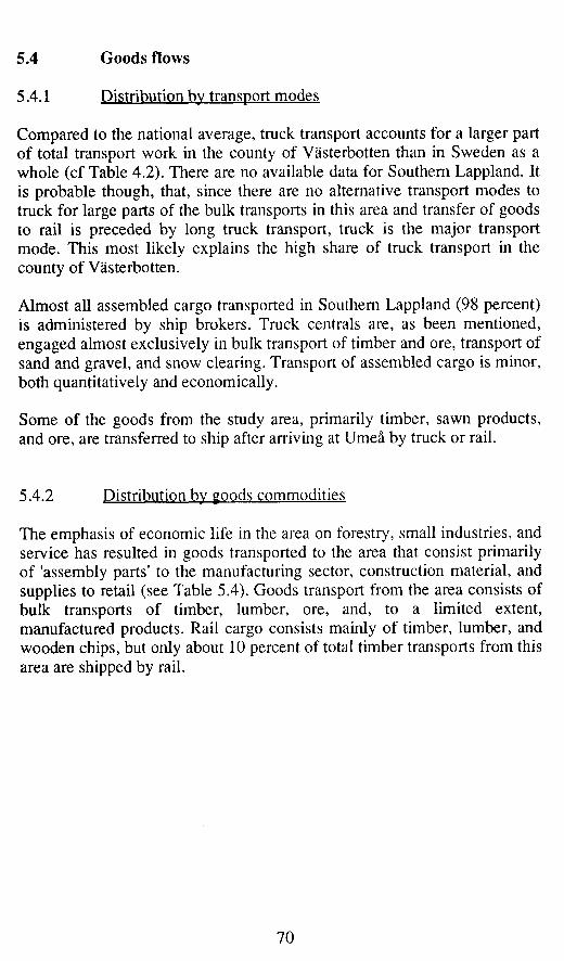
5.4 Goods flows

5.4.1 Distribution bv transport modes

Compared to the national average, truck transport accounts for a larger part of total transport work in the county of Västerbotten than in Sweden as a whole (cf Table 4.2). There are no available data for Southern Lappland. It is probable though, that, since there are no alternative transport modes to truck for large parts of the bulk transports in this area and transfer of goods to rail is preceded by long truck transport, truck is the major transport mode. This most likely explains the high share of truck transport in the county of Västerbotten.

Almost all assembled cargo transported in Southern Lappland (98 percent) is administered by ship brokers. Truck centrals are, as been mentioned, engaged almost exclusively in bulk transport of timber and ore, transport of sand and gravel, and snow clearing. Transport of assembled cargo is minor, both quantitatively and economically.

Some of the goods from the study area, primarily timber, sawn products, and ore, are transferred to ship after arriving at Umeå by truck or rail.

5.4.2 Distribution bv goods commodities

The emphasis of economic life in the area on forestry, small industries, and service has resulted in goods transported to the area that consist primarily of 'assembly parts' to the manufacturing sector, construction material, and supplies to retail (see Table 5.4). Goods transport from the area consists of bulk transports of timber, lumber, ore, and, to a limited extent, manufactured products. Rail cargo consists mainly of timber, lumber, and wooden chips, but only about 10 percent of total timber transports from this area are shipped by rail.

70

Table 5.4. Distribution of total truck goods by commodity in Southern Lappland in 1987.

Commodity 1000 ton

Assembled cargo of which foodstuff agriculture lumber, sawn products not specified

Bulk cargo of which ore petroleum timber

9671.2

29.5 12.5 52.6

9576.6 2460.0

500.0 70.0

1 890.0

TOTAL 12 131.2

Based on Nilsson & Westin, 1989a, 1989b

5.4.3 Distribution bv routes

Interaction between Southern Lappland and the coastal area of Umeå and the county of Västernorrland is considerable. A large part of the truck goods transported to and from the study area have their origin or destination in Umeå or pass the coastal area en route to the south of Sweden (see Map 5.2 and Table 5.5).

Goods transport was concentrated on certain major routes in 1987. Of assembled cargo transported to, from, and within Southern Lappland, about one fourth was transported from Lycksele to Umeå and further to southern parts of Sweden. Another fourth was transported from Umeå to Lycksele. A large part of the remaining half was due to the routes Umeå - Åsele and Umeå - Storuman.

71

Table 5.5. Distribution of assembled cargo by truck by Origin Destination in Southern Lappland in 1987.

Route 1000 tons

Within S Lappland To S Lappland of which Umeå - S Lappland Skellefteå - S Lappland Other V-botten - S Lappland S Sweden - S Lappland N Sweden - S Lappland

From S Lappland of which S Lappland - Other V-botten S Lappland - S Sweden S Lappland - N Sweden

S Lappland - Norway

38.2 6060.0

3537.7

35.3

5868.8 17.3 83.4

104.6 3372.5

60.6

83.9 6.6

Total 9671.2

Based on Nilsson & Westin, 1989b

Timber transports accounted for about 10 percent of the goods trucked from the area. Trucks operate on practically all roads. Timber transports were concentrated on major roads further east since the destinations for most timber were sawmills and paper mills in the Umeå-region and Västernorrland; demand of sawmills in the area was met (approximately 370.000 tons) and the remaining 1.5 million tons were shipped to other sawmills and paper-mills. Over 200 000 tons of timber were transported by truck to one of the four timber terminals in the area and then shipped by rail to the coast.

72

Map 5.2. Transport of assembled cargo and timber in the county of Västerbotten in 1987 Source: Nilsson & Westin, 1989b

73

6 PERCEPTION OF TRANSPORTATION CHARACTERISTICS

This chapter presents an experimental Stated Preference (SP) survey of transportation consumers' and transportation providers' valuation of a number of transportation characteristics. Various kinds of Stated Preferences including non-experimental surveys have been gathered and used transportation research. The experimental form of SP methods have been used frequently in transportation studies (Ben-Akiva & Lerman, 1985; Gärling, Uhlin & Widlert, 1989; Louviere, 1988) etc. The methods have also been applied in goods transportation studies, though to a less extent (TRANSEK, 1990).

In SP-methods the respondents are presented a set of hypothetical alternatives and, in contrast to Revealed Preference methods in which actual behavior is recorded, preferences are observed. Preferences do not necessarily express actual behavior since behavior is subject to various constraints (see chapter 3.3). This is a major criticism of SP-methods -people do not always do what they say. Such criticism does not disqualify SP-methods. Preferences are interesting if the objective is to estimate preferences and not actual behavior. If the hypothetical alternatives presented in an SP-study are realistic, SP data can be a reasonably accurate guide to underlying preferences (Wardman, 1988) and also give a hint on the direction of the revealed behavior.

6.1 Method

6.1.1 Stated-Preference methods

Methods for dealing with characteristics that cannot be directly observed are available today and allow the study of the consequences of hypothetical changes. These methods are called 'stated preferences' (SP). In contrast to 'revealed preference' methods13, SP-methods are based on hypothetical alternatives, some of which may or may not have occurred in reality.

• '3 Most studies of the choices and preferences of consumers and providers have employed methods based on observed actual behavior - so-called revealed preferences (RP). One advantage of the RP-method is that the connection between an observed actual behavior and the factors affecting this behavior can be analyzed directly. Thus, there is no need for hypothetical questions and the data collected refer to the respondents' performed actions.

74

This study analyzes the preferences and choices of consumers and providers of transportation services when some characteristics of the transportation system are changed. Some of the changes in the system may not have happened before, thus previous reactions of the actors could not be observed. Some of the changes may have occurred, but the actors' changed behavior was not recorded and cannot be reconstructed.

In SP-methods, respondents are presented a set of alternative situations described by characteristics that are varied on at least two levels. The respondents' beliefs, preferences, and intentions are measured with rating scales. Nominal, ordinal, interval, and ratio scales of measurement are used depending on the properties studied. The alternatives in this study are either ranked or rated, i.e., given scalar values. Since the alternatives presented vary in a strict order, their valuation can be estimated by a number of statistical techniques depending on the chosen scale. If the situations are ranked, logit analysis or MONANOVA analysis can be used. If the situations are valued on an interval or ratio level, traditional regression techniques can be used (Kroes & Sheldon, 1988). The level effects are given numerical values in terms of weights, monetary units, etc.

An advantage of SP-methods is that the characteristics can be described either verbally or visually to the respondents; it is not necessary to express the characteristics in numerical values (on an interval or ratio level). Another advantage of SP-methods is that situations that have not yet occurred can be valuated. SP-methods also allow the researcher to, a priori, define the variables and their levels and avoid problems of co-variation between characteristics. According to Kroes & Sheldon, a major disadvantage of the method is that it presumes that the rankings of situations given by the individual really represent the factual ranking in a real world situation. In this study preferences are used to estimate relative, rather than absolute, utility weights. SP-methods have proven to be useful under such instances.

Certain conditions must be fulfilled in order to successfully use SP-methods. The choice situation described must be seen as realistic and complete by each respondent. In addition, the characteristics presented must vary to such an extent that the levels can be separated

SP-methods are based on evaluation of various hypothetical alternatives. The task for the respondent is to evaluate a set of presented hypothetical alternatives with respect to e.g., preference. The first step is to define the characteristics and levels that describe the alternatives. For instance, a

75

goods transportation service can be defined by characteristics such as cost and time accuracy. Cost can, for example, take the levels (1) SEK 10, and (2) SEK 15, and time accuracy can take the levels (1) high, and (2) low. This gives a total of four possible alternatives to evaluate. Assume that n different characteristics are used to describe the J combined alternatives and let Uj denote the value of the j:th alternative. The utility (or preference) for the j:th alternative is then related to the levees of the characteristics (xjk) in a linear utility function (preference model). A commonly employed function is the linear additive compensatory model where ak denots the utility weight for characteristic k (Kroes & Sheldon. 1988);

U = OCjXj + c*2x2 +—ccnxn

where U = total utility. In this study it indicates preference for an

alternative and is expressed as probability of accepting the alternative.

xk = the value of characteristic k. ock = utility weights for characteristic k.

Other important issues are the choice of the context of the experiment, that is, whether the respondent is to express choices or preferences, and the measurement scale level of the dependent variable.

The next step, the experimental design, defines the combinations of the levels of the alternative transportation characteristics included in the experiment in such a way that they are uncorrelated. This objective could, however, result in a large number of alternatives if the number of characteristics and/or levels is too high and all possible combinations of all levels of each characteristic are included. If, for instance, there are three characteristics with three levels each, the number of situations in a full factorial design would be 33 or 27 alternatives.

Since it is usually advisable to let respondents evaluate a limited number of situations, generally 9 to 16, a "fractional factorial design" can be adopted. Only a selected number of all possible combinations are presented to the respondent with this design. Both the full factorial design and the fractional factorial design can be used to estimate the main effects, but all interaction effects can be estimated only when the full factorial design is used (ibid, 1988).

76

Should the number of alternatives be too large in a fractional design, it is possible to break down the exercise into smaller separate exercises. One common factor must be included in all exercises in order to link the utilities from each exercise.

The objective of this study was to estimate the sensitivity of different actors to changes in transportation service quality. An SP-method was used because some of the changes had not yet occurred, not all actors had been exposed to all changes to the same extent, and, finally, actual changes in individual characteristics had, in many cases, been relatively insignificant.

6.1.2 Choice of characteristics and levels

Two groups of actors were present in the modelled truck transportation market: transportation consumers and transportation providers. Transportation consumers included all companies in different industries in Southern Lappland that used truck for their goods transport.

The choice of characteristics was based on the intention to test characteristics that are integral parts of the Just-In-Time concept, and that had been found to be significant by other studies (Ballou, 1987; Storhagen, 1987; Tarkowski & Ireståhl, 1988; Areblom et al., 1990). According to these an application of JIT in a transportation perspective results in higher demands on distribution frequency, delivery times, time accuracy, goods safety, and correct information on deviations (see section 3.4). In a study of consumers' valuation of rail and truck transport the characteristics cost, frequency, delivery time, and time accuracy were tested (TRANSEK, 1990). Cost turned out to be the most significant characteristic.

Based on these findings consumers were asked to valuate five characteristics: transportation cost, delivery time, frequency, goods safety (loss and damage), and time accuracy (transit time variability). The objec­tive was, as stated above, to test characteristics that in other studies have been found important, thus the respondents were not given the opportunity to specify characteristics that they themselves judged to be important.

The consumers were a heterogeneous group in that they had various bases forjudging a transportation service depending on transported quantities and type of commodity. When testing the questionnaire, it proved unfeasible to specify the levels in numerical values with which all respondents could identify. Other studies (TRANSEK 1990) have shown that it is possible for

77

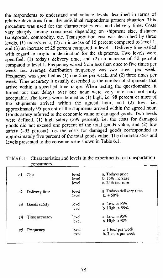
the respondents to understand and valliate levels described in terms of relative deviations from the individual respondents present situation. This procedure was used for the characteristics cost and delivery time. Costs vary sharply among consumers depending on shipment size, distance transported, commodity, etc. Transportation cost was described by three levels, (1) today's cost, (2) an increase of 15 percent compared to level 1, and (3) an increase of 25 percent compared to level 1. Delivery time varied with regard to origin or destination for the shipments. Two levels were specified, (1) today's delivery time, and (2) an increase of 50 percent compared to level 1. Frequency varied from less than once to five times per week and average distribution frequency was two times per week. Frequency was specified as (1) one time per week, and (2) three times per week. Time accuracy is usually described as the number of shipments that arrive within a specified time range. When testing the questionnaire, it turned out that delays over one hour were very rare and not fully acceptable. The levels were defined as (1) high, i.e. 98 percent or more of the shipments arrived within the agreed hour, and (2) low, i.e. approximately 95 percent of the shipments arrived within the agreed hour. Goods safety referred to the economic value of damaged goods. Two levels were defined, (1) high safety (>99 percent), i.e. the costs for damaged goods did not exceed one percent of the total goods value, and (2) low safety (-»95 percent), i.e. the costs for damaged goods corresponded to approximately five percent of the total goods value. The characteristics and levels presented to the consumers are shown in Table 6.1.

Table 6.1. Characteristics and levels in the experiments for transportation consumers.

cl Cost level a. Todays price level b. 15% increase level c. 25% increase

c2 Delivery time level a. Todays delivery time Delivery time level b. + 50%

c3 Goods safety level a. Low,^ 95% Goods safety level b. High, > 99%

c4 Time accuracy level a. Low, & 95% Time accuracy level b. High, *98%

c5 Frequency level a. 1 tour per week Frequency level b. 3 tours per week

78

Transportation services were provided by transports for hire and private truck. Transports for hire included ship brokers, truck centrals, and un­affiliated truckers.

The characteristics for providers to valuate was chosen to match the consumer experiment. When testing the questionnaire it turned out that the providers connected cost of a transportation assignment to revenue and vehicle utilization (quantity). The characteristic net cost and/or net revenue was tested but proved hard to understand and was rejected. Transportation providers were therefore asked to valuate six characteristics: cost, revenue, quantity (vehicle utilization), frequency, time accuracy (transit time variability), and goods safety (loss and damage). The providers also represented a heterogeneous group in that they operate on different levels -local, regional and national, have different business concepts (see section 6.2.2), and address different groups of customers. Thus, it proved useful to describe changes in cost and revenue in relation to present levels. Transportation cost was specified in the same three levels as for consumers, (1) today's cost, (2) an increase of 15 percent, and (3) an increase of 25 percent. Revenue was set at three levels, (1) today's revenue, (2) a decrease of 20 percent compared to level 1, and (3) an increase of 20 percent compared to level 1. The average total vehicle utilization rate was by providers estimated to a little less than 50 percent. Utilization referred to quantity and was measured as loaded quantity relation to total possible load. Since return cargoes are less frequent, quantity referred to one-way trips and was described by three levels, (1) 90 percent vehicle utilization, (2) 70 percent, and (3) 40 percent. The levels for frequency, time accuracy, and goods safety were identical to those presented to the consumers.

79

Table 6.2. Characteristics and levels in the experiments for transportation providers.

cl Cost level a. Todays cost S level b. 15% increase A level c. 25% increase F E c2 Revenue level a. Todays revenue T level b. - 20% Y level c. + 20%

G c3 Time accuracy level a. High,* 98% A level b. Low,^ 95% M E c4 Goods safety level a. High > 99%

level b. Low,^95%

F cl Cost level a. Todays cost R level b. 15% increase E level c. 25% increase Q U c2 Revenue level a. Todays revenue E level b. - 20% N level c. + 20% C Y c5 Quantity level a. 90% vehicle usage

level b. 70% vehicle usage G level c. 40% vehicle usage A

c. 40% vehicle usage

M c6 Frequency level a. 1 tour per week E level b. 3 tours per week

6.1.3 Experimental design

Consumers and providers of transportation services have different bases for assessing transportation services. They are a means of production for the transportation consumer and an item at sale for the transportation provider. This difference in the basic notion of the concept 'transportation service', means of production versus a product, required two, partly overlapping, experiments.

Given the number of characteristics and levels indicated in Tables 6.1 and 6.2, a full factorial design would have resulted in 3^x2^ or 48 alternatives

80

for the consumers to valuate. The number of alternatives presented was reduced to eight by using a fractional factorial design.

The number of possible alternatives for the providers to valuate meant that the experiment had to be divided into two smaller exercises. The first exercise, the frequency game, included cost, revenue, frequency and quantity characteristics. The second exercise, the safety game, included cost, revenue, time accuracy, and goods safety characteristics. Since the cost and revenue characteristics were included in both exercises, it was possible to express the preferences as well as the differences between levels in absolute terms. A full factorial design would have meant 33x21 or 54 alternatives in the frequency game and 32x2^ or 36 alternatives in the safety game. Applying a fractional factorial design resulted in nine alternatives for the transportation providers to valuate in both the frequency and the safety games (see Appendix B).

6.1.4 Survey

The consumer questionnaire was tested, revised, and tested again in the autumn of 1991. The questionnaires for transportation providers were tested in the early summer of 1991, revised, and retested. In addition to the hypothetical alternatives, the respondents were presented a number of background questions concerning the structure and size of their company. Shortened versions of the questionnaires are presented in appendices C and D.

The population 'transportation consumers' consisted of all companies, private as well as public, that used road transport for shipping goods. The sample was a two-step sample. In the first step a number of companies in each of the seven municipalities, proportional to the number of companies in each trade, were selected. Company was he sampling unit14 and from the public company catalogues 85 companies were selected on a random basis. Since there was no official source of companies that use trucks as a transport mode, the sample was extended with 85 alternative companies. An alternative company was used if the first-choice company did not employ truck services (and consequently did not belong to the population). The second step was realized in connection to the telephone interview (see page 83).

14This approach resulted in that many small companies with small shipmenst were drawn, and not rerepresentative for total goods flow.

81

The population 'transportation providers' consisted of all distributors of goods (excluding bulk transports of gas, timber, ore, and so on) to, from, and within the studied area. Close to 80 percent of the goods carried in 1990 were shipped by transport for hire (SM T 30, 9302). Previous studies (SPK 1991:3) have revealed that the majority of long-distant transports are administered by ship brokers with 'ASG' and 'Bilspedition' as the dominant brokers. Short-distant transport is, to a large extent, carried out by freight companies, administered either by truck centrals or internally. Private trucks constitute a larger number of vehicles, but carry less goods quantities than trucks for hire.

The provider population was stratified into three strata. The first strata consisted of the four ship brokers that operated in the area. The second strata included the truck centrals and freight companies not affiliated to brokers or truck centrals in the study area and the truck centrals in Umeå and Skellefteå who operate in the area on a less regular basis (10 companies). The third strata consisted of five companies, mainly wholesalers, with their own transportation fleet (private truck). The sample drawn included 19 transportation providers (see Table 6.3).

The consumers and providers were geographically widely scattered. For economic and time-saving reasons, a combined mail and telephone survey method was employed. A letter of introduction and the questionnaire were sent to the respondents in a sealed envelope. The letter described the study and the respondent was asked not to open the envelope until he/she was approached by an interviewer via telephone. The interviews were carried out by experienced and trained interviewers. The experiment design meant that all respondents in each actor group were given the same alternatives to evaluate, although the order varied.

A letter of introduction and the questionnaire were sent to the transportation consumers in November, 1991. The letter was addressed to the transport manager, if one existed, or to the managing director. A few days after the respondent had received the letter, he/she was contacted by an interviewer. The respondent was asked first if truck transport was used. If the answer was no, the company was excluded from the survey. A new letter was sent out to a matching alternative company in the same municipality and trade. If the company used trucking services, the respondent was asked if it was a convenient time for an interview lasting approximately 30 minutes, or if an appointment for an interview could be made. When the interview began, the respondent was asked to open the sealed envelope. He/she could then see the alternatives to be evaluated.

82

Table 6.3. Sample size and response rate.

Sample No of Response-size resp. rate, percent

CONSUMERS 85 76 89% of which by the municipality of

78% Sorsele 9 7 78% Storuman 12 11 92% Malå 8 7 88% Lycksele 25 23 92% Vilhelmina 13 12 92% Åsele 9 8 89% Dorotea 9 8 89%

of which by industry 10 Agric. & forestry 12 10 83%

95% Manufacturing 19 18 83% 95%

Construction 9 7 78% Retail 10 10 100% Transport. Communie 6 4 67% Private service 12 11 92% Public service 17 16 94%

PRODUCERS 19 15 77% of which Ship brokers 4 3 75% Truck centrals 10 7 70% Private trucks 5 5 100%

The questionnaire presented to transportation consumers was in two parts. The first part was a traditional Stated-Preference exercise. The respondent was asked to think of an existing major truck transportation service to or from the company. The transport was defined by five characteristics: transportation cost, delivery-time, goods safety, time accuracy, and frequency. The respondent's task was, first, to indicate on a nine-point rating scale (where 1 indicated very bad and 9 very good) how he/she perceived this transportation service. Second, the respondent indicated on a 100-point scale (indicating percent) the probability of accepting the transportation service. The end-points were defined as not probable at all (0 percent chance of accepting) and absolutely probable (100 percent chance of accepting).

The second part of the interview consisted of questions about the company: company size in terms of number of employees and turn-over, what transport modes were used, extent of truck transport in terms of tonnage

83

and frequency, transportation costs in relation to turnover, available transportation providers, and perception about the existing transport situation.

The questionnaire for transportation providers was also in two parts. Part one contained a traditional Stated-Preference exercise. The respondent was asked to imagine a transportation assignment to or from the study area, a distance of approximately 200 km one way. The assignment demanded a truck with a three-axel trailer. Loading at five different places was scheduled to take one hour and unloading at 10 customers was calculated to take two hours. There were no immediate possibilities for a return cargo15. The transportation assignment was defined by six characteristics: transportation cost, revenue (the price the customer was charged), quantity, frequency, goods safety, and time accuracy. The respondent's task was then to indicate on a nine-point rating scale (where 1 indicated very bad and 9 very good) how he/she perceived this transportation assignment. The respondent also indicated on a 100-point scale the probability of accepting the assignment. The end-points were defined as not probable at all (0 percent chance of accepting) and absolutely probable (100 percent chance of accepting).

The second part of the interview consisted of questions about the transportation company: local and regional market share, competition, company policy with respect to business concept and profit margins, and, finally, questions about what measures the company would take if goods quantities on single routes were to decrease.

The response rate was satisfactory, as shown in Table 6.3. In general, respondents had no problems understanding the alternatives. However, some respondents, mainly shipping agents for whom freight discounts of up to 70 percent were not unusual, regarded the difference in levels of the factor cost as very small while free trucking associations, who generally employed very small discounts, regarded the difference in levels as large.

The hypothetical transportation assignment varied with the respondents. Shipping agents and trucking associations/free truckers in the coastal area were to imagine a transportation assignment to the study area. The distance was set to 200 kilometers one-way, loading at five depots in Umeå was estimated to take one hour, and unloading at 10 customers in the study area was estimated to take two hours. Shipping agents and trucking associations/free truckers in the study area were to imagine a transportation assignment from the study area, approximately 200 kilometers one-way, loading in the study area at five depots was estimated to take one hour, and unloading at 10 places in Umeå was set to two hours. The assignment for 'company trucks' was a 200 kilometer trip to the study area.

84

6.2 Results

6.2.1 Transportation consumers

Background As Figure 6.1 shows, most companies were small, seven out of ten had less than five employees. Among the medium-sized companies with 50-100 employees were two manufacturing companies and two public service institutions. One manufacturing and one förrest company represented companies with more than 100 employed.

16T

14-

Q. E

IwlglJwiBIMH 1 3 5 7 9 12 16 18 20 23 35 70 90 150

2 4 6 8 10 15 17 19 21 25 60 72 100 No of employees

Figure 6.1. Distribution of companies in the study with respect to number of employees.

A majority of the companies had a turnover of one to four million SEK (less than 1 million US$). The range was, as shown in Figure 6.2, 1 to 170 million SEK.

In addition to using trucks as a mode of transport, more than half of the companies used public bus and postal services to a minor extent. Very few (less than 20 percent) used air or rail transport. The companies received goods twice a week on average and sent goods once a week. Transport costs corresponded to up to 40 percent of production value, but were only five percent on average.

85

IIII IIÌIBIIIi iw i ì h w 9 11 14 16 23 30 45 70 150

8 10 12 15 20 25 38 62 120 170 Turnover in mill SEK

Figure 6.2. Distribution of companies in the study with respect to turnover.

Results The consumers were presented five characteristics in one experiment. Four of the characteristics were identical with those presented to the transportations providers while the fifth concerned delivery-time. The mean value of how the transportation service was perceived in terms of good or bad and the probability of accepting the service was calculated for each level of the five characteristics. As shown in Table 6.4, the consumers assigned relatively low 'satisfaction' values to the different characteristics and levels. Further, the respondents were sensitive to changes in transportation cost and frequency. They also perceived high time accuracy to be better than low time accuracy and high goods safety to be better than low safety.

The differences between respondents within different industries are not significant. Respondents within 'construction' assigned higher 'satisfaction' values compared to other industries. Respondents in 'agriculture' indicated practically no sensitivity towards cost increases and increased delivery time, while they were more sensitive than most other respondents for changes in time accuracy. A few discrepancies can be noted, however. Respondents in the trades 'agriculture', 'transport & communication' and 'private service' indicated higher average values for increased costs than they did for today's level, i.e., they perceived higher costs to be better than

86

lower costs. This is assumed to result from the choice of method and how the alternatives presented can be conceptualized, rather than the respondents' true perception. This will be discussed further in chapter 7.

Table 6.4. Mean values of transportation consumer's perception of transportation characteristics in Southern Lappland in 1991.

Characteristic Level All Agric. Manu- Constr Retail Transp. Private Public forr fact. comm. service serv.

Cost Todays 3.4 3.0 3.3 4.1 4.4 3.5 2.9 3.0 + 15% 3.1 3.1 2.8 3.9 3.3 2.4 3.1 3.0 + 25% 2.4 2.9 1.9 2.6 3.1 3.0 2.0 2.3

Del. time Todays 3.4 3.1 2.9 4.1 3.9 3.1 3.3 3.4 + 50% 2.8 2.9 2.6 3.3 3.6 3.0 2.2 2.5

Frequency 3/week 3.8 3.7 3.1 4.8 4.8 3.8 3.3 3.6 1/week 2.1 2.0 2.3 2.1 2.3 2.0 1.9 1.8

Time accuracy High 3.4 3.7 2.7 4.0 4.4 3.5 2.9 3.2 Low 2.8 2.4 2.7 3.3 3.3 2.7 2.5 2.6

Goods safety High 3.5 3.4 3.0 4.2 4.3 3.6 3.1 3.4 Low 2.7 2.7 2.6 3.2 3.3 2.7 2.5 2.6

No. of companies 76 10 18 7 10 4 11 16 No. of cases 608 80 144 56 80 32 88 128

The values were obtained/expressed on an equal-interval rating scale ranging from 1 (very bad) to 9 (very good).

Despite the low estimates of satisfaction on the different factors, a majority of respondents (seven out of ten) found present transport conditions satisfactory and two out of ten even found present conditions very good. Most respondents, three out of four, stated that they had other transport options if the present provider disappeared from the market.

As indicated in Table 6.5, the consumers assigned very low probability values to accepting a transportation service. There were some significant differences between industries, but not with regard to company size or municipality (location). The respondents in 'retail' often indicated higher chances of accepting services than those in other industries, while the lowest chances were found in 'manufacturing' and 'public services'.

87

Table 6.5. Mean values of transportation consumer's probability of accepting transportation services in Southern Lappland in 1991.

All Agric. Manu- Constr Retail Transp. Private Public Characteristic Level for. fact. comm. service serv.

Cost Todays .27 .24 .22 .32 .42 .34 .30 .18 + 15% .25 .23 .19 .32 .26 .29 .35 .22 + 25% .18 .22 .09 .19 .27 .30 .19 .14

Delivery time Todays .24 .23 .15 .29 .32 .33 .30 .18 + 50% .22 .23 .17 .25 .32 .31 .22 .15

Frequency 3/week .33 .31 .22 .43 .49 .42 .35 .28 1/week .15 .15 .14 .15 .16 .22 .21 .08

Time accuracy High .27 .29 .19 .31 .39 .36 .31 .18 Low .22 .17 .18 .26 .29 .28 .26 .18

Goods safety High .30 .27 .21 .38 .40 .38 .31 .26 Low .21 .20 .16 .24 .31 .28 .26 .13

No. of companies 76 10 18 7 10 4 11 16 No. of cases 608 80 144 56 80 32 88 128

The values were obtained/expressed on an equal-interval rating scale ranging from 0 (not probable) to 1 (absolutely probable).

The highest level of acceptance for today's transportation costs was given by respondents in the 'retail' group. Retail customers also turned out to be the most sensitive group for cost increases, and an increase of 25 percent led to a drop in probability of accepting the service by .14. Respondents in the trade 'agriculture and forestry' were least sensitive to increased costs.

Respondents in all groups, with the exception of 'private services', stated that they were fairly indifferent to changes in move-time. Changes in goods safety and time accuracy affected the consumers more than changes in move-time. Considering that the increased demands for JIT-transport are primarily associated with manufacturing, it seems contradictory that respondents in the trade 'manufacturing' were least sensitive to lower time-accuracy.

However, regardless of industry, the respondents, particularly the 'retail' group, were sensitive to lower frequency. The probability of accepting a

88

delivery frequency of once a week was estimated at .16 while the probability estimate for three deliveries per week was .49. Representatives of 'manufacturing' and 'public services' assigned low estimates (.22 and .27 respectively) to a frequency of three times per week.

In general, transportation consumers assigned very low estimates to the existing situation. The probability estimate for accepting the present transportation situation, i.e., what they are actually paying for and accepting today, was only .27. However, this discrepancy between revealed and stated preference should not be interpreted as if SP-methods are unreliable. Stated preferences indicate what is preferred. Reality imposes a number of restrictions on behavior when action occur. The low estimates for the present transportation situation can be regarded as an indication that present conditions are unsatisfactory.

An OLS regression analysis16 showed that frequency was the most important characteristic for transportation consumers. As Table 6.6 indicates, the characteristics frequency, delivery time and time accuracy were significant. Increasing of frequency from once per week to three times per week would result in an increased probability to accept the service by .19. Differences exist among different industries. Respondents in 'private service' were more sensitive to changes in cost of transport and goods safety. A cost increase of 25 percent would result in a .17 drop in the probability of accepting the service and a change from low to high goods safety would lead to an increase in the probability of accepting by .16.

' ̂ The purpose of the regression model is to estimate the utility function, in which utility is measured as the probability of accepting a transportation service.

89

Table 6.6. Estimates of coefficients in the regression model for transportation consumer's probability of accepting a transportation service in Southern Lappland in 1991.

Charact. All Agricult. Manufac- Construc- Retail Transp. Private Public Level forestry hiring tion comm. service service

Freq. 3/week 19.4*** 19.9 8.1 28.6* 28.3** 17.5 7.3 33.7***

Cost +15% -.6 2.6 -2.5 -13.9 -13.4 -7.5 .4 10.5

Cost +25% • 00

* 2.1 -13.1* 1.0 -13.9 -7.5 -16.8 5.8 Del.time +50% -8.5*** -4.7 -3.5 9.0 -10.3 10.0 5.0 9.5

Time acc. high 9.1*** 17.2 3.3 -15.3 15.8* -5.0 -12.3 12.3*

Goods safe, high 5.8 1.6 4.7 13.4 2.9 12.5 16.4 -3.4

r2 .170 .190 .101 .381 .300 .275 .154 .292

No. of companies 76 10 18 7 10 4 11 16 of cases 608 80 144 56 80 32 88 128

The values were obtained/expressed on an equal-interval rating scale ranging from 0 (not probable) to 100 (absolutely probable).

p < .05 p < .01 p < .001

6.2.2 Transportation providers

Background The three groups of transportation providers were very different with respect to vehicle fleet size, turnover, transported quantity, business concept, etc. Ship brokers had large fleets, 50 to 100 trucks, at their disposal. Their turnover cannot be compared to the other groups, and they work primarily on the national and regional levels. The brokers each estimated their market share in the county of Västerbotten (regional market) at 40 to 50 percent.

Truck centrals handle only minor amounts of assembled cargo and their revenue emanates from other types of transport assignments. Private trucks operate on an entirely different basis. Their vehicle fleet is usually small,

90

generally they do not show a turnover specifically for transportation, and they only serve a selected group.

Results The mean values of how a transportation assignment was perceived in terms of good or bad and the probability of accepting the assignment, was calculated in the same way as for transportation consumers. The valuation of the characteristics in terms of good or bad (satisfaction) is shown in Table 6.7. As might be expected, a cost increase resulted in lower satisfaction. Increased revenue, increased quantity, and higher frequency were also perceived to be better than unvaried or decreased revenue, lower quantity, and lower frequency.

Table 6.7. Mean values of transportation provider's perception of transportation characteristics in Southern Lappland in 1991.

Charact. All Ship Truck Private Level suppl. brokers centrals trucks

Cost Todays 5.9 7.8 5.5 5.4 + 15% 4.3 5.8 3.3 4.8 + 25% 3.7 4.5 2.6 4.6

Revenue -20% 3.0 4.5 2.1 3.4 Todays 4.5 5.5 3.4 5.4 + 20% 6.4 8.0 5.9 6.0

Quantity 90% 5.4 6.9 3.8 7.0 Quantity 70% 4.7 5.7 3.8 5.4 40% 3.8 5.5 4.0 2.2

Frequency 3/week 5.0 6.9 4.6 4.5 Frequency 1/week 4.4 5.6 3.5 5.1

Time accuracy High 4.0 5.0 3.0 4.7 Time accuracy Low 5.3 7.0 4.5 5.3

Goods safety High 5.0 6.6 4.1 2.6 Goods safety Low 4.6 5.9 3.7 4.9

no of companies 15 3 7 5 no of cases 270 54 126 90

The values were obtained/expressed on an equal-interval rating scale ranging from 1 (very bad) to 9 (very good).

91

All three groups of transportation providers perceived low time accuracy to be better than high time accuracy. Nevertheless, they indicated that the customer's demand for a high or low level of time accuracy was not essential. The providers operated mostly with fixed timetables and tried to avoid deviations from these. Since a cargo usually contained goods to or from several customers, it was impossible to discriminate between different demands on time accuracy and the providers claimed that all customers got the highest level of time accuracy regardless of what they paid for.

The same line of reasoning was valid for goods safety. The providers strived to minimize damages since it would take too much time and money to settle any damage claims and safe transportation was usually part of the business concept of the various transportation providers. The results reflect these news as assignments with high safety demands were perceived to be somewhat better than those with low safety demands. However, the providers were less sensitive to changes in this factor than the consumers.

Finally, the valuation of the different characteristics and levels varied between the three strata of providers. In general, ship brokers assigned higher values to the different levels than did respondents from truck centrals and private trucks.

The estimated probabilities of accepting an assignment when the characteristics vary are presented in Table 6.8. The probability of accepting varied among the three strata of providers. Ship brokers turned out to be less sensitive to increases in transportation costs than respondents in truck centrals and private trucks. In addition, ship brokers were also more inclined than the other two groups to accept a transportation assignment despite a reduction in revenue. The brokers justified their position as a result of their national operations and their business concept of managing all kinds of assignments despite the type of goods or geographic origin and destination. If a broker could not live up to his business concept, a competing broker would soon take an increased market share. Moreover, the ship brokers worked with cross-subsidies. Potential economic losses emanating from rural transport were generally smaller than the profits made from more goods extensive routes.

The truck centrals and unaffiliated freight companies operated on an entirely different basis. Their geographical operating area was, with very few exceptions, restricted to a municipality. The respondents in this group stated that assignments outside the operating area had to yield a profit in order to be acceptable, and they did not actively strive to achieve such

92

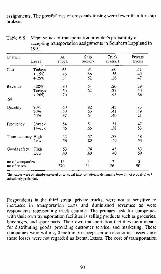
assignments. The possibilities of cross-subsidising were fewer than for ship brokers.

Table 6.8. Mean values of transportation provider's probability of accepting transportation assignments in Southern Lappland in 1991.

Charact. Level

All suppl.

Ship brokers

Truck centrals

Private trucks

Cost Todays .65 .91 .60 .57 + 15% .46 .66 .36 .49 + 25% .38 .52 .26 .47

Revenue -20% .30 .54 .20 .29 Todays .50 .62 .37 .60 + 20% .70 .93 .66

.64

Quantity 90% .60 .82 .45 .73 70% .50 .65 .41 .59 40% .37 .64 .40 .21

Frequency 3/week .54 .81 .51 .47 1/week .46 .65 .38 .53

Time accuracy High .42 .57 .33 .48 Low .56 .82 .49 .53

Goods safety High .53 .74 .45 .53 Low .49 .69 .40 .50

no of companies 15 3 7 5 no of cases 270 54 126 90

The values were obtained/expressed on an equal-interval rating scale ranging from 0 (not probable) to 1 (absolutely probable).

Respondents in the third strata, private trucks, were not as sensitive to increases in transportation costs and diminished revenues as were respondents representing truck centrals. The primary task for companies with their own transportation facilities is selling products such as groceries, beverages, and spare parts. Their own transportation facilities are a means for distributing goods, providing customer service, and marketing. These companies were willing, therefore, to accept certain economic losses since these losses were not regarded as factual losses. The cost of transportation

93

was included in the price of the product they were selling and they covered all expenses in the long run. If their own transportation services become too expensive and the price of their product uncompetitive, they would buy transportation services or somehow coordinate transport with other companies.

The two experiments have been linked together in a regression model. It was assumed that the variance in the two experiments differed, and therefore a WLS (Weighted Least Square) method was employed. Ship brokers and truck centrals/unaffiliated freight companies were sensitive for cost increases and increases in revenue as indicated in Table 6.9. A 25 percent increase in cost would result in 47 and 33 percent decreases, respectively, in the probability of accepting an assignment. Respondents in the private trucks group, on the other hand, were most sensitive to a major decrease in quantity. A decrease from 90 to 40 percent vehicle utilization would mean a 42 percent decrease in the probability of accepting the assignment. The overall differences between the three strata were significant (p<.01).

94

Table 6.9. Estimates of coefficients in the regression model for transportation provider's probability of accepting a transportation assignment in Southern Lappland in 1991.

Characteristic Level

All suppl.

Ship brokers

Truck centrals

Private trucks

Frequency, 3t/week -3.4 1.0 1.6 -20.0 Quantity, 70% -9.2 -17.4 -3.3 -20.7*** Quantity, 40% -17 4*** -18.9 -4.3 -52.0*** Revenue, -20% -24.6*** -15.4 -22.0*** -35.3*** Revenue, +20% 16.9*** 2i 7*** 20.3*** g 4*** Cost, +15% -14 9*** -16.8*** -16.8*** -9.4 Cost, +25% -24.8*** -32 0*** -29.6*** -9.6 Goods safety, high -2.7 2.5 3.1 2.0 Time accuracy, high -9.3* -15.1 -8.8 -8.2

r2 .461 .435 .612 .337

no of companies 15 3 7 5 no of cases 270 54 126 90

The values were obtained/expressed on an equal-interval rating scale ranging from 0 (not probable) to 1 (absolutely probable).

p < .05 p < .01 pc.001

Finally, the respondents were asked what measures would be taken should the goods quantity on a route fall below a critical limit, first temporarily and then in the long term. Respondents representing ship brokers and truck centrals stated that, in the short term, they would traffic the route and cover possible economic losses through cross-subsidies. In the long term ship brokers would change frequency, while truck centrals would try to coordinate the transport assignment with others or close traffic on the route. Respondents from the private truck group were more inclined to buy the transportation service from other providers or coordinate transport with other companies in both the short and long terms.

95

6.2.3 Performance of the regression models

A regression model was used to test the transportation characteristics in explaining the probability of accepting a transportation service. The regression model showed low revalues which indicate a high unexplained variance.

Differences between individual respondents account for the low revalues. Testing for individual effects showed that there are significant (pc.001) differences on a disaggregated level, but these differences evened out when the individual responses are aggregated.

Another possible reason for the low revalues is that the characteristics in the model do not fully explain the probability of accepting a service. Transportation characteristics other than those tested in the model may be important. As discussed in chapter 3.4., extra services such as packaging, customs procedures, warehousing, and information have become more important for customers. Testing the importance of other transportation characteristics is a future task. It may be also that other types of characteristics predominate. One group of transportation providers stated that, despite bad conditions for an assignment, they would accept it. Accepting all assignments would be in line with their business concept.

6.3 Changes in the transportation market

In this chapter SP-data are used for estimating changes in goods flows. The purpose is to evaluate hypothetical effects of changes of transportation characteristics. The estimated changes in the transportation market also provide a practical illustration of the valuations of different characteristics and to compare the transportation consumers and transportation providers. The examples presented below are very hypothetical. As will be further discussed in chapter 7, other studies show that one has to be careful when applying SP-data in estimating demand or in forecasting (Kroes & Sheldon, 1988; Wardman, 1988). Individuals' stated preferences among hypothetical scenarios are, however, a reasonably accurate guide to true underlying preferences (Wardman, 1988).

Assuming that the preferences for different characteristics correspond to a real choice situation the changes in the transportation market in terms of goods quantities are estimated. The estimations are based on the probability

96

values presented in tables 6.5 and 6.8. They are adjusted to 1.0 for current conditions, and the goods quantities are equal to present conditions at this level.

6.3.1 Transportation consumers

The consumers were most sensitive to changes in distribution frequency. A decrease from three times to once per week would mean a reduction of more than half in total goods quantity (see Table 6.10). A cost increase of 25 percent and lower goods safety would each result in a reduction in transported goods quantity by about one third.

Almost half of the total quantity transported was composed of goods to or from public service facilities. Respondents in this sector were very sensitive to lower frequency and a change of distribution frequency from three times to once per week would result in a 70 percent decrease in their shipments. Further, respondents in the public service sector were more sensitive to lowered goods safety than to cost increases. Respondents in the manufacturing sector were the only group that was more sensitive to a 25 percent cost increase than to lowered frequency. The manufacturing sector was the second largest transport consumer. A 25 percent increase in transportation costs would result in a 1.2 million tons reduction in goods, which is one tenth of the total transported goods quantity.

Table 6.10. Effects of changes on transportation characteristics based on transportation consumers' valuation in million tons.

Characteristic All Agric. Manu- Constr. Retail Transp. Priv. Public Change for. fact. comm. serv. serv.

Todays level 9.67 0.01 2.05 0.88 0.03 0.86 1.44 4.40 Cost + 15 percent 8.28 0.01 1.77 0.88 0.02 0.74 1.44 4.40 + 25 percent 6.48 0.01 0.84 0.52 0.02 0.76 0.91 3.42

Delivery time + 50 percent 8.38 0.01 2.05 0.76 0.03 0.81 1.05 3.67

Frequency 1.26 1 time/week 4.20 0.01 1.30 0.31 0.01 0.45 0.86 1.26

Time accuracy low 8.93 0.01 1.94 0.74 0.02 0.67 1.20 4.40

Goods safety low 6.17 0.01 1.56 0.55 0.02 0.63 1.20 2.20

97

Routes affected to a larger extent by changes in the transportation characteristics would be the same as those defined as major goods routes in chapter 3, e.g. Lycksele - Umeå - South of Sweden, Umeå - Lycksele, Umeå - Åsele, and Umeå - Storuman. About three quarters of the total goods quantity in the manufacturing sector and also three quarters of private service goods were found on these routes. Approximately 90 percent of the goods in the public service sector were transported on these routes.

In conclusion, the regression analysis on the probability of accepting a transport showed that frequency, time accuracy, and delivery time were significant for the consumers (cf Table 6.6). When estimating changes of goods quantities, a drop of frequency would cause the largest effect with a decrease of over 50 percent. Lower goods safety and a 25 percent cost increase would cause larger effects on the quantity than would lower time accuracy and increased delivery time.

Significant charact. Goods flow

1 rank frequency frequency 2 rank time accuracy goods safety 3 rank delivery time cost

6.3.2. Transportation providers

A cost increase would have the largest impact on the total goods flow for the transportation providers. An increase of 25 percent would result in a reduction from 9.7 million tons to 5.5 million tons. i.e. 40 percent. Higher demand on time accuracy from low to high would result in a 30 percent reduction in goods quantity (see Table 6.11).

Most (98 percent) of the assembled cargo transported in the area was shipped through ship brokers. Thus, their preferences have great impact on the total goods flow. A cost increase of 25 percent would result in a reduction from the 9.5 million tons transported today to 5.4 million tons, while a 15 percent cost increase would mean a reduction to 6.9 million tons. The second most obvious effect would be caused by higher demands on time accuracy.

98

Table 6.11. Effects of changes on transportation characteristics based on transportation providers' valuation, in million tons.

Characteristic Change

Total Ship brokers

Truck centrals

Private trucks

Todays level 9.67 9.51 0.12 0.04 Cost +15 percent 7.01 6.90 0.07 0.04 +25 percent 5.53 5.44 0.05 0.04

Revenue -20 percent 8.36 8.28 0.06 0.02

Quantity 0.10 0.03 70% 7.67 7.54 0.10 0.03

40% 7.53 7.42 0.10 0.01 Frequency

0.09 0.03 1 time/week 7.75 7.63 0.09 0.03 Time accuracy

0.08 0.04 high 6.73 6.61 0.08 0.04 Goods safety low 9.01 8.87 0.10 0.04

Major routes that would be affected by a cost increase are those from Lycksele to southern parts of Sweden via Umeå, and from Umeå to Lycksele, Åsele and Storuman respectively. Ship brokers administer transport of most kinds of commodities and a cost increase would affect the transportation options for all kinds of customers. The exception is foodstuffs and agricultural commodities which are delivered mainly by private truck.

A cost increase would also affect truck centrals in the sense that the goods quantities would be reduced. A 25 percent cost increase would reduce transported quantities by more than half to 60.000 tons. Should the truck centrals act in accordance with their stated probabilities of accepting it would have a large impact on the goods flows from Holmsund (the port of Umeå) to Lycksele and from Storuman to Umeå since half of the total quantity was transported on these routes. The remaining 60.000 tons were divided on many small shipments and transported on routes within municipalities or between neighbouring municipality centers.

In conclusion, the regression model indicated that increased costs, changed revenues, and a drop of transported quantity (vehicle utilization) from 90 percent to 40 percent were significant. Increased costs for the providers would also have the largest impact on the goods quantity. Higher demands

99

on time accuracy would have the second greatest impact on the goods quantity.

1 rank 2 rank 3 rank

revenue cost

quantity

cost time accuracy quantity

It is obvious that transportation consumers in a sparsely populated area valuated transportation characteristics differently, from transportation providers. Consumers were more sensitive to lowered distribution frequency, lower time accuracy, and increased delivery time than were the providers. The providers were most sensitive to increased costs and lower revenues.

6.4 Stated Preference as a method

The second aim of this study was to test Stated-Preference methods as tools for valuating goods transportation characteristics.

Several studies have emphasized the importance of great care in defining and describing the characteristics and levels. The characteristics and levels used in this study were tested and revised and retested. The respondents indicated that they understood the characteristics and levels presented to them, and that the alternatives (transportation services and assignments) were realistic. Although the alternatives represented hypothetical situations, many of them 'could happen'. For example, the adding of a 12 percent VAT on transport in January 1991 and increased fuel prices help to picture relative large changes. Therefore, relative levels such as 15 and 25 percent cost increases, could easily be conceived.

In a few cases the results differ from what can be expected. An example is that a 25 percent cost increase was perceived to be better than an increase by 15 percent (cf Table 6.4). It can be argued that this can be a result of inadequate design of characteristics and levels. As stated above, the respondents gave no indications of such misunderstanding. However, the method assumes that individuals are rational and consistent in their choices.

100

The contradictory reults may be a consequence of our lack to be completely rational.

In response to a direct question a majority (90 percent) of the consumers stated that they were satisfied, or very satisfied, with their present transport situation. However, the probabilities of accepting different levels, and even present levels, were generally low. This can be an indicator that the methods are unsuitable in estimating preferences. It is known from other studies that individuals tend to over- or understate their responses under experimental conditions. This is not a major problem as long as the objective is to estimate the relative utility or importance of characteristics. Should the intention be to predict behavior based solely on SP-data great caution must be taken. Then it is advisable to use SP-data in conjunction with RP-data (Kroes & Sheldon, 1988).

101

7 SUMMARY AND CONCLUSIONS

Round the world there are large sparsely populated areas with small and scattered population centers, and the distances between centers within these areas as well as to more populated urban areas are long. Long distances and a limited supply of transportation options contribute to high costs for transportation to, from and within sparsely populated areas. Goods quantities on individual routes are small when compared to other areas. This restricts distribution frequency since it is not economically feasible for transportation providers to traffic all routes with high frequency. For business life in sparsely populated areas, high costs, limited supply, long delivery times, and low frequency are obstructions, to being competitive. Thus, JIT-transport is not easily achieved in sparsely populated areas.

The aim of the study is to analyze how consumers and providers of goods transportation services in a sparsely populated area valuate different transportation characteristics and how these valuations might affect the total goods flows and the flows on different routes. An additional methodological aim is to test the Stated-Preference methods as tools for valuating transportation characteristics.

Two hypotheses were tested in the study. The first hypothesis, HI, was that consumers of transportation services in sparsely populated areas assign greater importance to frequency and transportation cost then they assign to the Just-In-Time characteristics delivery time, time accuracy, and goods safety. This hypothesis can only partly be verified. Results from the SP-study indicate that frequency was perceived as the most important characteristic: an increase of frequency from once to three times per week would increase the probability of accepting a service by .19. Based on this study the assumption that cost was one of the most important characteristics can be rejected: time accuracy and delivery time were perceived to be more important than cost.

The second hypothesis, H2, was that providers of transportation services are most sensitive to increased costs and/or lower revenues. This hypothesis was verified: a cost increase by 25 percent or a decrease of revenue by 20 percent were each perceived to result in .24 decrease in probability of accepting an assignment.

102

Stated Preference as a method There are some contradictions in the results of the Stated Preference study. Consumers in the industry 'transport & communication' perceive a 25 percent cost increase to be better than a 15 percent cost increase (see Table 6.4). Another contradiction is that providers in truck centrals state that lower vehicle utilization is better than higher (see Table 6.7).

This raises the question if the SP-method is an adequate tool for valuating transportation characteristics. Studies like Kroes & Sheldon (1988) have concluded that SP is useful when estimating relative utility weights. An important issue is whether respondents can evaluate a set of alternatives presented to them by expressing their preferences properly on the measurement scale. Efforts must be made to describe the factors properly. The alternatives presented must seem realistic and the researcher must insure that the respondents understand the alternatives. It is also important that the levels are expressed accurately. Absolute values for cost, revenue, quantity, and delivery time varied among the respondents in this study. Hence, the levels of such characteristics were described in relative terms, e.g., a 15 percent increase, in order to reduce the problem of individual bases for making statements.

Estimations of the respondents' assessment and stated probability of accepting transportation services showed low values. Even today's levels had low acceptance values. In response to a direct question about how they perceived the present transport situation, the consumers stated that they found it satisfactory or very satisfactory. One reason for these seemingly contradictory results is that the respondents are generally dissatisfied, but the threshold for not accepting is raised when they face a real situation. The stated preferences in this case are bad estimations of their revealed preferences. However, the SP-method is more valid if the purpose is to compare the valuation of a number of characteristics.

Despite some contradictory results the study indicates that the SP-method is a robust tool for valuation of goods transportation characteristics. The tests carried out within the framework of this study imply that SP-methods can be used to estimate relative utility values even when the list of options is deemed not fully adequate.

It would be appropriate in future studies to adopt a more heuristic approach and ask a set of actors to define their own list of important characteristics. This is important especially in areas and/or sectors where significant restrictions or limitations affect market mechanisms. An SP-study could

103

then be made to valuate characteristics and service performance of the market.

Implications for sparsely populated areas Increased application of a JIT-concept in various industries has resulted in a change in consumers' requirements on transportation services. As the results above imply consumers in sparsely populated areas assign great importance to the JIT characteristics frequency, delivery time, time accuracy, and goods safety. This raises the question if transportation providers can respond to consumer requirements. In the SP-exercise the providers indicated that cost and revenue were important characteristics. Increased requirements of frequency, time accuracy, and goods safety would not result in significant decreases in probability of accepting. This 'insensitivity' for JIT-characteristics is, according to the providers, a result of regarding demands on short delivery times, high time accuracy, and high goods safety as easy to respond to and not a question of cost. Striving to minimize deviations and provide good services is generally part of the providers' business concept. Requirements on higher frequency is also quite possible to respond to but is an economic question. In conclusion, providers respond to the demands from consumers. The consumers, in a direct question, stated that they are satisfied, or very satisfied, with their present transport situation (in principal hired truck).

A majority of the goods is transported by ship brokers. The brokers assigned higher probabilities of accepting transportation assignments than truck centrals and private trucks. One explanation for this is their business concept of providing all kinds of transportation services and covering all routes. Another explanation is the possibilities of cross-subsidies. Transport of assembled goods on minor routes, such as in Southern Lappland, account for a very small part of the brokers total operation. A large part of the brokers' assignments are transport on major routes, e.g., Umeå-Stockholm, Stockholm-Göteborg, and Stockholm-Malmö. Another important part is bulk transport of timber, ore, petroleum, etc. Profits arising from these major assignments are used to cover potential deficits arising from traffic in sparsely populated areas. Thus, consumers in sparsely populated areas benefit from the present situation with cross-subsidizing.

It can be questioned if this cross-subsidy policy will last. A current trend in economic life is deregulation and/or privatization of both private and public companies. The deregulation of air traffic resulted in new entries on

104

primarily major profitable air routes. As the possibilities of cross-subsidising were reduced traffic on a number of minor air lines was closed. The privatization of the former Swedish Telephone Company resulted in readjustment of telephone fees: each part of the operation has to cover its own cost and i.e., the cost for short distance calls has increased while that of long distance calls has decreased.

A similar development in trucking, with different routes being separate economic units, could jeopardize transport possibilities in sparsely populated areas. For brokers, however, the competitive advantages of managing transport on all routes exceed the economic deficits of transport in sparsely populated areas. In addition, the trucking industry was deregulated in the early 1980s when entry restrictions were eased. After a few years the number of trucks were lower than before the deregulation, and the major national brokers had strengthened their position.

In conclusion, goods transport conditions need not be an obstruction for development of industry in sparsely populated areas. Goods transportation systems are more favorable to sparsely populated areas than many other systems.

105

106

APPENDIX A. Counties and provincial capitals of Sweden

BD

Östersund^ ^

Harnosaa

AB Stockholms län C Uppsala län D Södermanlands län E Östergötlands län F Jönköpings län G Kronobergs län H Kalmar län I Gotlands län K Blekinge län 1 Kristianstads län M Malmöhus län N Hallands län O Göteborgs och Bohus län P Älvsborgs län R Skaraborgs län S Värmlands län T Örebro län U Västmanlands län W Kopparbergs län X Gävleborgs län Y Västernorrlands län 2 Jämtlands län AC Västerbottens län BD Norrbottens län

wW

Uppsala v»

Västerås

Karlstad Stockholm

Örebro

Nyköping Marieslid unkopm

Q /vaners-

Visby

Jonkop Goteborg®^ P

Karlskrona Kristianstad

Malmö (

107

108

APPENDIX B. Experimental design using a fractional factorial design.

CONSUMER EXPERIMENT

Experi- Characteristic ment no CI C2 C3 C4 C5

1 0 0 0 0 0 2 0 1 1 1 1 3 1 0 1 1 1 4 1 1 1 0 0 5 2 0 1 0 1 6 2 1 0 1 0 7 1 0 1 1 0 8 1 1 0 0 1

The levels were randomly set as;

CI, cost a=0 b=l C2, delivery time a=0 b=l C3, goods safety a=l b=0 C4, time accuracy a=0 b=l C5, frequency a=0 b=l

109

PRODUCER EXPERIMENT

Frequency game

Experi- Characteristic ment no CI C2 C3 C4

1 0 0 0 0 2 0 1 1 0 3 0 1 2 1 4 10 11 5 1 2 2 0 6 1 2 0 0 7 2 0 2 0 8 2 1 0 1 9 2 2 1 0

The levels were randomly set as;

CI, cost a=0 b=l c=2 C2, revenue a=2 b=0 c=l C3, quantity a=0 b=l c=2 C4, frequency a=0 b=l

Safety game

Experi­ment no

Characteristic Cl C2 C5 C6

1 2 3 4 5 6 7

0 0 0 1 1 1 2 2 2

0 1 2 0 1 2 0 1 2

0 1 0 1 1 0 0 0 1

0 0 1 1 0 0 0 1 0

The levels were randomly set as;

CI, cost a=2 b=0 C2, revenue a=l b=2 C5, time accuracy a=l b=0 C6, goods safety a=l b=0

c=l c=0

110

APPENDIX C. SP-questionnaire for transportation consumers

INSTRUCTION

We would like to ask You some questions on how You valuate goods transports to or from Your company.

Consider a recent major truck transport of goods to or from Your company. In each of the following pages a hypothetical transportation service is described in terms of

COST, refers to what Your company pays for the transportation service)

DELIVERY TIME, for door-to-door transport

GOODS SAFETY, refers to how large part of the goods that is free of damage in relation to total goods value). High safety (>99 percent) indicates that the cost for damages does not exceed 1 percent of the goods value. Low safety 95 percent) indicates that the cost for damages does not exceed 5 percent of the goods value.

TIME ACCURACY, refers to how often the goods arrives on schedule. High time accuracy (>98 percent) indicates that 98 percent or more of the deliveries arrive within the hour. Low time accuracy (<^95 percent) indicates that 95 percent of the deliveries arrive within the hour.

FREQUENCY, refers to number of deliveries per week.

A value for each characteristic is defined for every hypothetical transportation service. Assuming that in all other aspects the transportation service is unchanged, how would You rate the described transport in terms of good or bad? Indicate by circling a number on the following scale:

Very Very bad 123456789 good

If You conceive the transportation service to be very good, mark the number 9. If You perceive the service to be very bad, indicate number 1. Should You consider the transportation service to be neither good nor bad, indicate number 5.

We would also like to know how probable You think it is that Your company would accept a transportation service with these conditions/ should everything else be unchanged. Indicate Your answer on the following scale:

Not probable Absolutely at all o 10 20 30 40 50 60 70 80 90 100% probable

If You think that Your company would not accept the service, indicate 0%. If You think that Your company with absolute certainty would accept the service, indicate 100%. If You think the chance of accepting is 50 percent, indicate 50%.

I l l

Consider a recent main truck transport with goods to or from Your company. The conditions are:

#1

Cost for Your company

I i 1 + 15% 1 i i i

Delivery time door-to-door

1 1 1 Today's | i i I

Goods safety Undamaged goods in relation to total goods value

1 1 i i 1 High 1 1 (> 99%) 1 1 1 I

Time accuracy Delivery within the hour

1 1 1 1 1 Low 1 1 (^95%) 1 i

Frequency Number of deli­veries per week

1 1 1 1 1 3 per week |

How do You valuate this transportation service for Your company?

Very Very bad 123456789 good

How probable is it that Your company would accept a transportation service with these conditions?

Not probable Absolutely at all o i o 2 0 3 0 4 0 5 0 6 0 7 0 8 0 9 0 100% probable

112

APPENDIX D. SP-questionnaire for transportation producers

INSTRUCTION We would like to ask You some questions about how You valuate a number of transportation characteristics.

Imagine that a customer asks for a transportation service, with the following specifications: - a one-way transport of 200 kilometres to Southern Lapland - assembled cargo - the goods quantity means a truck with a 3-axel trailer - loading in Umeå at 5 places, expected to take 1 hour - un-loading at 10 places in Southern Lapland, approx. 2 hours - no immediate return cargo.

In each of the following pages a hypothetical transportation service is described in terms of

COST, refers to what it actually costs Your company to carry out the assignment)

REVENUE, refers to what the customer pays QUANTITY, alludes to vehicle utilization FREQUENCY, refers to number of deliveries per week. GOODS SAFETY, refers to how large part of damages the customer

accepts. High safety (>99 percent) indicates that the cost for damages does not exceed 1 percent of the goods value. Low safety (-:95 percent) indicates that the cost for damages does not exceed 5 percent of the goods value.

TIME ACCURACY refers to how large part of the deliveries that must arrive on schedule. High accuracy (»98 percent) indicates that 98 percent or more of the deliveries arrive within the hour. Low accuracy (~:95 percent) indicates that 95 percent of the deliveries arrive within the hour.

A value for each characteristic is defined for every hypothetical transportation assignment. Assuming that in all other aspects the transportation is unchanged, how would You rate the described assignment in terms of good or bad? Indicate by circling a number on the following scale:

Very Very bad 123456789 good

If You conceive the transportation assignment to be very good, mark the number 9. If You perceive the assignment to be very bad, indicate number 1. Should You consider the transportation assignment to be neither good nor bad, indicate number 5.

We would also like to know how probable You think it is that Your company would accept a transportation assignment* with these conditions, should everything else be unchanged. Indicate Your answer on the following scale:

Not probable Absolutely at all o io 20 30 40 50 60 70 80 90 100% probable

If You think that Your company would not accept the assignment , indicate 0%. If You think that Your company with absolute certainty would accept the assignment, indicate 100%. If You think the chance of accepting is 50 percent, indicate 50%.

113

FREQUENCY GAME

Imagine : - a one-way transport of 200 kilometres to Southern Lapland - assembled cargo - the goods quantity means a truck with a 3-axel trailer - loading at 5 places in Umeå, expected to take 1 hour - un-loading at 10 places in Southern Lapland, approx. 2 hours - no immediate return cargo.

# 1 - 1

1 1 Cost

1 1 1 Today1 s |

1 for Your company i 1 I

1 Revenue 1 1 i 1

1 what Your company 1 - 20% 1 1 charges the customer 1 1

I

1 Quantity 1 1 1 1

1 Vehicle utilization I 9 0% 1 1 one-way trip 1 1

I 1 Frequency

1 1 1 1

1 Number of deli­ 1 3 per week | veries per week

1 1

How do You valuate this transportation service for Your company?

Very Very bad 123456789 good

How probable is it that Your company would accept a transportation service with these conditions?

Not probable Absolutely at all o i o 2 0 3 0 4 0 5 0 ' 6 0 7 0 s o 9 0 100% probable

114

SAFETY GAME

Imagine : - a one-way transport of 200 kilometres to Southern Lapland - assembled cargo - the goods quantity means a truck with a 3-axel trailer - loading at 5 places in Umeå, expected to take 1 hour - un-loading at 10 places in Southern Lapland, approx. 2 hours - no immediate return cargo.

# 2 - 1

1 Cost for Your company

1 + 15%

Revenue what Your company charges the customer

+ 20%

Goods safety Undamaged goods in relation to total goods value

Low ( ̂ 95%)

Time accuracy Delivery within the hour

Low ( ̂ 95%)

How do You valuate this transportation service for Your company?

Very Very bad 123456789 good

How probable is it that Your company would accept a transportatior service with these conditions?

Not probable Absolutely at all o io 20 30 40 50 60 70 80 90 100% probable

115

116

REFERENCES

Abrahamsson, H. & Sandahl, F. (1990): Internationella transporter och Spedition. (International transport and shipping). Liber, S Sandby.

Andersson, Å. E. & Strömquist, U. (1988): K-Samhällets Framtid. (The Future of the C-society). Prisma, Värnamo.

Areblom, P.-A., Havner, E. & Hägertz, T. (1990): Mindresändningar i Just-In-Time-flöden. (Smaller Shipments in JIT-flows.) TFB-rapport 1990:13.

Ballou, R.H. (1987): Basic Business Logistics. Prentice-Hall. Englewood, N.J.

Bamford, H. & Robinson, C.G. (1978): Geography of Transport. Macdonald and Evans, Plymouth.

Barnes, T J. (1988): Rationality and relativism in economic geography. In Progress in Human Geography, vol 12 no 4.

Befolkningen. Sveriges National Atlas, 1991. (The Population. Swedish National Atlas).

Ben-Akiva, M. & Lerman, S.R. (1985): Discrete Choice Analysis: Theory and Application to Travel Demand. MIT Press, Cambrigde.

Bird, J. (1989) The Changing Worlds of Geography. Clarendon Press, Oxford.

Borg, J., Wandel, S. & Ågren, B. (1992): On Measuring Macro Logistic Costs and Performance In Sweden and Other Countries. Paper presented at the 6th World Conference on Transport Research (WCTR), Lyon, France July 1992.

Bovy, P.H.L. & Stern, E. (1990): Route Choice: Wayfinding in Transport Networks. Kluwer, The Netherlands.

Bowersox, D.J., Smykay, E.W. & LaLonde, B.J. (1968): Physical Distribution Management. MacMillan, New York.

Dillard, D. (1969): Västeuropas och Förenta staternas ekonomiska historia. (Economic development of the North Atlantic Community). Liber. Lund.

117

Eliot Hurst, M.E. (1974): The Geographie Study of Transportation, Its Definition, Growth, and Scope. In Eliot Hurst (ed): Transportation Geography, McGraw-Hill, New York.

Friedrich, C.J. (1928): Alfred Weber's Theory of the Location of Industries. The University of Chicago Press, Chicago.

Gilg, A. (1985): An Introduction to Rural Geogràphy. Edward Arnold, London.

Golledge, R.G. & Couclelis, H. (1984): Positivist philosophy and research on human spatial behavior. In Saarinen, T.F., Seamon, D. & Sell, J.L. (red) Environmental Perception and Behavior. University of Chicago, Research paper no 209.

Golledge, R.G. & Rushton, G. (1984): A Review of Analytic Behavioural Research in Geography. In Herbet, D.T. & Johnston, R.J. (eds) Geography and the Urban Environment Progress in Research and Applications, Vol VI. John Wiley & Sons.

Gärling, T., Uhlin, S. & Widlert, S. (1989): Validering av Stated Preference Metoder för Mätning av Resenärers Värdering av Kollektivtrafikens Standard. (Validity of Stated Preference Methods for Travelers' Evaluation of Public Transport Systems). TRUM-Rapport 1989:2, Umeå.

Haggett, P. (1965): Locational Analysis in Human Geography. Edward Arnold, London.

Hansson, L. (1991): The Pricing of Air Pollution In the Swedish Transport Policy. Paper presented at the Transportation Research Board's 70th Annual Meeting, Washington, D.C.

Heckscher, E.F. (1907): Till belysning af järnvägarnas betydelse för Sveriges ekonomiska utveckling. (The role of railways in the economic development in Sweden). Stockholm.

Hoyle, B.S. & Knowles, R.D. (1992): Transport Geography: an introduction. In Hoyle, B.S. & Knowles, R.D. (eds) Modern Transport Geography. Belhaven Press, London.

118

Hoyle, B.S. & Smith, J. (1992): Transport and Development. In Hoyle, B.S. & Knowles, R.D. (eds) Modern Transport Geography. Belhaven Press, London.

Hultén, S. (1991): Infrastruktur, industriell omvandling och produktivitet. In Produktivitetsdelegationen Infrastruktur och produktivitet (Infrastructure and productivity). Allmänna Förlaget, Stockholm.

Hägerstrand, T. (1991): What About People in Regional Science. In Carlestam, G. & Sollbe, B. (eds) Om tidens vidd och tingens ordning. BFR.

Infrastrukturen - förvaltning, kommunikationer, energi. Sveriges National Atlas, 1991. (The Infrastructure - administration, communications, energy, Swedish National Atlas).

Johnston, R.J. (1986): Philosophy and Human Geography. 2nd edition. Edward Arnold, London.

Johnston, R.J. (1991): Geography and Geographers. 4th edition. Edward Arnold, London.

Kroes, E.P. & Sheldon, R.J. (1988): Stated Preference Methods. An Introduction. In Journal of Transport Economics and Policy, vol 22 no 1.

La Londe, B., Grabner, J.R. & Robeson, J.F. (1976): Integrated Distribution Systems: a Management Perspective. In van Buijtenen, P. (ed) Business Logistics, Martinus Nijhoff, The Hague.

Louviere, B.J. (1988): Conjoint Analysis Modelling of Stated Preferences. In Journal of Transport Economics and Policy, vol 22 no 1.

Morrill, R.L. (1974): The Spatial Organization of Society. Duxbury Press, Belmont, Cal.

Munro. J.M. (1974): Depressed Regions and Transportation Investments. In Eliot Hurst, M.E. (ed) Transportation Geography. McGraw-Hill.

Nilsson, P. & Westin, K. (1989a): Godstransporter î Västerbottens och Norrbottens län - teknisk rapport. (Goods transports in Västerbotten and Norrbotten - technical report). GERUM arbetsrapport, Umeå.

119

Nilsson, P. & Westin, K. (1989b): Godstransporter i Västerbottens och Norrbottens län - teknisk rapport. (Goods transports in Västerbotten and Norrbotten - results). GERUM, Umeå.

Pirenne, H. (1936): Economic and Social History of Medieval Europe. 8th impression 1965. Routledge & Kegan Paul Ltd, London.

Sack, R.D. (1973): A Concept of Physical Space in Geography. In Geographical Analysis 5, pp 16-34.

Sarv, H., Ericsson, D. & Bäckman, G. (1985): MA idag. Materialadministration och utveckling. (Business logistics of today). Liber, Stockholm.

Smith, A. (1904): The Wealth of Nations. Cannan, E. (ed). Methuen, London.

Statistics Sweden: SCB: Statistiska Meddelanden (Notices) AM60 SM 9301 AM60 SM 9401 T30 SM 9201 T45 SM 9201 T50 SM 9201 T55 SM 9201 Årsbok för Sveriges kommuner 1991 (Yearbook for the Swedish municipalities 1991) Årsbok för Sveriges kommuner 1992 (Yearbook for the Swedish municipalities 1992) Statistical Yearbook 1963 Statistisk Årsbok 1982/83 (Statistical Yearbook 1982/83) Statistisk Årsbok 1993 (Statistical Yearbook 1993)

Storhagen, N.G. (1987): Materialadministration - grunder och möjligheter. (Business logistics - basics and possibilities). Liber, Kristianstad.

Swedish Competition Authority (1991): SPK: Pris och konkurrens 1991:3. (Price and competition).

Taffee, E.J. & Gauthier, H.L. Jr (1973): Geography of Transportation. Prentice- Hall, Englewood Cliffs NJ.

120

Tarkowski, J. & Ireståhl, B. (1988): Transportadministration. (Transport administration). Studentlitteratur, Lund.

Trafikpolitiken inför 90-talet; Proposition 1987/88:50. (Government Bill on Transport Policy for the 1990s). Stockholm.

TRANSEK (1990): Godskunders värderingar. (Transportation consumers' valuation.) Banverket, Planeringsavdelningen.

Transport Board (1983a): Transportrådet: Transporter i Sverige Del IIA -Godstransporter. (Transports in Sweden Part IIA - goods transports). TPR-Rapport 1983:3, Transportrådet.

Transport Board (1983b): Transportrådet: Transporter i Sverige Del IIA Bilaga - Godstransporter. (Transports in Sweden Part IIA Appendix - goods transports). TPR-Rapport 1983:3, Transportrådet.

Transport Board (1983c): Transportrådet: Transporter i Sverige Del Hl -Godstransportprognos. (Transports in Sweden Part III - forecast on goods transports). TPR-Rapport 1983:5, Transportrådet.

Transport Board (1986): Transportrådet: Godsterminaler - nuläge och strukturella förändringar. (Terminals - present condition and structural changes). TPR-Rapport 1986:1, Transportrådet.

Transport Board (1990a): Transportrådet: Kvartalsstatistik 1990:1-2. (Statistics).

Transport Board (1990b): Transportrådet: Kvartalsstatistik 1990:3. (Statistics).

Törnqvist, G. (1963): Studier i I ndustrilokalisering. (Studies of location of industry). Meddelanden från geografiska institutionen vid Stockholms universitet, nr 153. Esselte, Stockholm.

Ullman, E.L. (1974): Geography as Spatial Interaction. In Eliot Hurst, M.E. (red) Transportation Geography. McGraw-Hill.

Wardman, M. (1988): Comparison of RP and SP Models of Travel Behaviour. In Journal of transport economics and policy, vol 22 no 1.

121

Westin, K. & Waara, R. (1985): Gods- och personbefordran med samma buss. (Coordinated goods and passenger transportation by bus). TRUM Arbetsrapport 1985:01, Umeå.

Westlund, H. (1992): Kommunikationer, tillgänglighet, omvandling. (Comminications, Accessibility, Transformation). Umeå Studies in Economic History no 16, Umeå.

Ågren, B. (1983): Kostnader för transport-, hanterings- och lagringsverksamhet i olika branscher - mätning av effektivitet och rationaliseringsmöjligheter. (Costs for transportation, materials management and warehousing in different trades). Linköping University.

122

Geographical Reports

1. Lindberg, Olof: Ubiquity and areal transport costs. 1965.

2. Häggström, Nils: Norrland's direct foreign trade 1850-1914. (Academic thesis). 1971.

3. Lindberg, Olof: Urban settlement and income distribution. A geographic study of the city of Umeå. 1972.

4. Rice, John G: Patterns of ethnicity in a Minnesota county, 1880-1905. 1973

5. Weissglas, Gösta: Studies on service problems in the sparsely populated areas in northern Sweden. (Academic thesis). 1975.

6. Layton, Ian G: The evolution of Upper Norrland's ports and loading places 1750-1976. (Academic thesis). 1981.

7. Layton, Ian G: Trade, resource utilization and economic change in the Lule valley, northern Sweden, c. 1550-1900. (Forthcoming).

8. Abrahamsson, Kurt V (ed): Northern Land Use and Grazing Animals. Proceedings from a UNESCO - MAB Northern Science Network Symposium. 1985.

9. Malmberg, Gunnar: Metropolitan Growth and Migration in Peru. (Academic thesis). 1988.

10. Sivertun, Åke: Geographical Information Systems (GIS) as a Tool for Analysis and Communication of Complex Data. (Academic thesis). 1993.

11. Weissglas, Gösta (ed): Planning a High-Resilience Society. Papers and proceedings from the Lövånger Symposium. 1994.

12. Westin, Kerstin: Valuation of Goods Transportation Characteristics. - A Study of a Sparsely Populated Area. (Academic thesis). 1994.

-< — <" gg -o . V

Department of Geography Umeå university, Sweden

ISBN 91-7174-909-8 ISSN 0349-4683