Generic Energy Demand Profile Generation - Strath Energy Demand Profile Generation ... supply/demand...

Department of Mechanical and Aerospace Engineering

Generic Energy Demand Profile Generation

Author:

Raheal McGhee

Supervisor:

Prof. Joe Clarke

A thesis submitted in partial fulfilment for the requirement of the degree

Master of Science

Sustainable Engineering: Renewable Energy Systems and the Environment

2012

2

Copyright Declaration

This thesis is the result of the author’s original research. It has been composed by the

author and has not been previously submitted for examination which has led to the

award of a degree.

The copyright of this thesis belongs to the author under the terms of the United

Kingdom Copyright Acts as qualified by University of Strathclyde Regulation 3.50.

Due acknowledgement must always be made of the use of any material contained in,

or derived from, this thesis.

Signed: Raheal McGhee Date: 10th September 2012

3

Abstract

Electrical and thermal demand profiles were collected and analysed for a range of different

buildings. Various factors were calculated for each of these buildings, such as their annual

energy consumption per floor area, and were utilised to generate Generic Profiles for each

building type such as Schools, Offices, and Houses etc. A Profile Library was designed

which stores and provides relevant information and demand profiles of all buildings used in

this project. This database also allows the demand data for each individual building to be

exported which can then be readily imported into energy-matching tools such as Merit.

A Generic Electricity Consumption Calculator was developed which can be used to

approximate the annual electrical consumption of a specific type of building by scaling a

number of features such as floor area and average daily occupancy.

A taxonomy was created to illustrate the demand profiles contained within the Profile

Library. A range of categories were included to allow easier and clearer understanding.

For the demonstration of the latest version of Merit, two demand profiles from buildings

James Young and John Anderson, part of the University of Strathclyde, were used for

supply/demand energy matching analysis. The supply profiles used in conjunction with these

demand profiles consisted of data generation from Wind Turbines and Solar PV Cells. It was

found that, with the generated supply profiles, James Young received an optimal Match Rate

of 44.11 % when combined with 10 Proven WT600 Wind Turbines. John Anderson received

an optimal Match Rate of 2.83 % with 10 Proven WT600 Wind Turbines and 10 165 W

Sharp Poly Solar Panels.

4

Acknowledgements

I would like to thank my supervisor Prof. Joe Clarke for his support and guidance throughout

my project. I would also like to thank Jun Hong for his assistance with Merit and help

regarding the database.

Special thanks go to the following Councils/Organisations who provided me with their data

and, if mentioned, their representatives with whom I had contact:

Aberdeenshire City Council - Brian Smith; Angus City Council; Argyle & Bute Council;

BAA - Peter Chalmers; Bartlett School of Graduate Studies, University College London;

data.gov.uk; Building Research Establishment; Dumfries & Galloway Council - David Moss;

East Renfrewshire Council - Hamish Campbell; Edinburgh City Council - Alastair Maclean;

Fife Council - Janet Archibald, Helen McLaren, Laura Murray & Steven Lyzcak; Glasgow

City Council - Gavin Slater; Highland Council - Murdo MacLeod; Inverclyde Council; NHS

Greater Glasgow & Clyde; North Lanarkshire Council; South Ayrshire Council; UK Energy

Research Centre Energy Data Centre (UKERC-EDC); University of Strathclyde Estates -

Ross Simpson; West Lothian Council.

Finally, I would like to thank my family and friends for their continuous support and

encouragement throughout my project.

5

Contents

Declaration ................................................................................................................................ 2

Abstract ..................................................................................................................................... 3

Acknowledgements ................................................................................................................... 4

Contents..................................................................................................................................... 5

List of Figures, Graphs and Tables ........................................................................................ 8

Chapter 1: Introduction ........................................................................................................ 11

1.1 Overview ................................................................................................................ 11

1.2 Scope and Objective ............................................................................................... 13

Chapter 2: Literature Review ............................................................................................... 15

2.1 Renewable Electricity ............................................................................................. 15

2.2 Renewable Heat ...................................................................................................... 18

2.3 Energy-Saving Buildings ....................................................................................... 21

2.4 SMART Buildings .................................................................................................. 23

2.5 Hybrid Renewable Energy Systems ....................................................................... 24

2.6 Merit – Supply/Demand Energy Matching Tool .................................................... 25

2.6.1 Overview ................................................................................................. 25

2.6.2 Procedure ................................................................................................. 26

Chapter 3: Collection, Collation and Interpolation of Electrical/Thermal Demand

Profiles .................................................................................................................................... 28

3.1 Collection and Collation of Demand Data ............................................................. 28

3.2 Interpolation of Demand Data ................................................................................ 29

3.2.1 Format of Data ......................................................................................... 29

3.2.2 Missing Individual Data Cells ................................................................. 31

3.2.3 Missing Daily Data .................................................................................. 33

3.2.4 Missing Weekly/Monthly Data ............................................................... 35

3.2.5 Inaccurate or Unreliable Data .................................................................. 37

Chapter 4: Generic Demand Profile Generation ................................................................ 40

4.1 Care Home .............................................................................................................. 41

4.1.1 Generic Care Home ................................................................................. 42

4.2 Community Centre ................................................................................................. 43

4.2.1 Generic Community Centre ..................................................................... 44

6

4.3 Emergency Services ............................................................................................... 45

4.3.1 Generic Emergency Services ................................................................... 45

4.4 Hall/Venue .............................................................................................................. 46

4.4.1 Generic Hall/Venue ................................................................................. 47

4.5 High/Secondary School .......................................................................................... 48

4.5.1 Generic High/Secondary School ............................................................. 49

4.6 Houses .................................................................................................................... 51

4.6.1 Generic Houses ........................................................................................ 53

4.7 Leisure Centre ........................................................................................................ 54

4.7.1 Generic Leisure Centre ............................................................................ 55

4.8 Library .................................................................................................................... 56

4.8.1 Generic Library ........................................................................................ 57

4.9 Maintenance Services ............................................................................................. 58

4.9.1 Generic Maintenance Services ................................................................ 58

4.10 Museum/Art Gallery ............................................................................................. 59

4.10.1 Generic Museum/Art Gallery ................................................................ 60

4.11 Nursery/Primary School ....................................................................................... 60

4.11.1 Generic Nursery/Primary ....................................................................... 61

4.12 Office .................................................................................................................... 64

4.12.1 Generic Office ....................................................................................... 65

4.13 Specialist School .................................................................................................. 67

4.13.1 Generic Specialist School ...................................................................... 67

4.14 Transport .............................................................................................................. 68

4.14.1 Generic Transport .................................................................................. 69

4.15 University of Strathclyde ...................................................................................... 70

Chapter 5: Profile Library .................................................................................................... 73

5.1 Introduction Worksheet .......................................................................................... 74

5.2 Demand Profile Worksheets ................................................................................... 74

5.3 Supply Profile Worksheet ...................................................................................... 74

5.4 Taxonomy ............................................................................................................... 74

Chapter 6: Generic Electricity Consumption Calculator ................................................... 76

Chapter 7: Analysing the University of Strathclyde with Merit ........................................ 78

Chapter 8: Conclusions and Future Work .......................................................................... 82

8.1 Conclusion .............................................................................................................. 82

7

8.2 Future Work ........................................................................................................... 83

References ............................................................................................................................... 84

Appendix 1: Map of Scottish Regions .................................................................................. 90

Appendix 2: Location of Milton Keynes, England .............................................................. 91

8

List of Figures

Figure 1. Example of required format of demand profile.

Figure 2. Example of a missing individual data cell.

Figure 3. Example of calculated approximation on the missing individual data cell.

Figure 4. Example of a missing data cluster.

Figure 5. Example of calculated approximation on the missing data cluster.

Figure 6. Example of missing weekly/monthly data.

Figure 7. Example of calculating the average percentage difference.

Figure 8. Example of inaccurate data.

Figure 9. Example of calculated approximation on inaccurate data.

Figure 10. Example of unreliable data.

Figure 11. Percentage consumption for University buildings of overall campus demand.

Figure 12. Snapshot of the Demand Profile – Buildings Worksheet in the Profile Library.

Figure 13. Snapshot of the Generic Profile Taxonomy.

Figure 14. Snapshot of the Generic Electricity Consumption Calculator in the Profile Library.

Figure 15. Annotated snapshot of matching interface in Merit.

Figure 16. Optimal match found for James Young.

Figure 17. Optimal match found for John Anderson.

List of Graphs

Graph 1. Growth in electricity generation from renewable sources since 2010.

Graph 2. Electricity demand by sector in 2010.

Graph 3. Input of renewable energy fuel-types in 2010.

Graph 4. Annual electrical consumption/floor area for each Care Home.

Graph 5. Annual electrical consumption/floor area for each community centre.

Graph 6. Annual electrical consumption/floor area for each emergency service.

Graph 7. Annual electrical consumption/floor area for each Hall/Venue.

Graph 8. (LOW) annual electrical consumption/floor area for each High School.

9

Graph 9. (MEDIUM) annual electrical consumption/floor area for each High School.

Graph 10. (HIGH) annual electrical consumption/floor area for each High School.

Graph 11. Generic annual electrical consumption/floor area for each dwelling-type.

Graph 12. Annual electrical consumption/floor area for each Leisure Centre.

Graph 13. Annual electrical consumption/floor area for each Library.

Graph 14. Annual electrical consumption/floor area for each Maintenance Service.

Graph 15. (LOW) annual electrical consumption/floor area for each Nursery/Primary School.

Graph 16. (MEDIUM) annual electrical consumption/floor area for each Nursery/Primary

School.

Graph 17. (HIGH) annual electrical consumption/floor area for each Nursery/Primary School.

Graph 18. (LOW) annual electrical consumption/floor area for each Office.

Graph 19. (MEDIUM) annual electrical consumption/floor area for each Office.

Graph 20. (HIGH) annual electrical consumption/floor area for each Office.

Graph 21. Annual electrical consumption/floor area for each Specialist School.

Graph 22. Annual electrical consumption/floor area for each Transport.

Graph 23. Annual electrical consumption/floor area for each University building.

List of Tables

Table 1. World power generation by wind technology.

Table 2. Electricity generation by common renewable technologies.

Table 3. Predicted electricity consumption for future scenarios.

Table 4. Heat generation by common renewable technologies.

Table 5. Type, no. of electrical/thermal and location of demand profiles for given building.

Table 6. Care Home Data.

Table 7. Community Centre Data.

Table 8. Emergency Services Data.

Table 9. Hall/Venue Data.

Table 10. High/Secondary School Data.

Table 11. House Data.

Table 12. Generic House Data.

10

Table 13. Leisure Centre Data.

Table 14. Library Data.

Table 15. Maintenance Services Data.

Table 16. Museum/Art Gallery Data.

Table 17. Nursery/Primary School Data.

Table 18. Office Data.

Table 19. Specialist School Data.

Table 20. Transport Data.

Table 21. University of Strathclyde Data.

11

Chapter 1: Introduction

1.1 Overview

Renewable energy, a phenomenon which enables diverse forms of energy to be converted and

utilised, is captured by a range of technologies such as wind turbines, solar PV cells, heat

pumps etc (Abulfotuh, 2007). There is also widespread misconception amongst the general

population who believe that there were sparse amounts of renewable technologies from the

1990s compared to 2000 and beyond (Mitchell & Connor, 2004). Taking wind power

generation as an example to highlight this misunderstanding, the following table shows the

amount of World Power Generation from 1990 to 2008. It can be seen that in the 10 years

from 1990 to 2000, there has been an increase of 30.2 % of global power generation via wind.

From 1990 to 2008, the power produced rose to more than two-thirds of the initial value in

1990 to 70.7 %. This shows that there were still a significant amount of renewable wind

technologies almost 20 years ago even though a large number of people were not aware of it.

Year World Power

Generation (TWh)

% Increase of World Power

Generation compared to 1990

1990 11,821 -

2000 15,395 +30.2

2005 18,258 +54.5

2008 20,181 +70.7

Table 1. World power generation by wind technology (Energy in Sweden facts and figures 2010).

Renewable energy has become a mainstream topic in newspapers, magazines, television etc

in recent times mainly due to increasing energy costs and Government carbon-emission

targets. With the surge of renewable technologies being developed and built within the last 20

years has caused a fair proportion of the public to favour renewable energy and would prefer

nuclear power to be removed (Krohn & Damborg, 1999; Pidgeon et al, 2008).

All available renewable technologies have both positive and negative factors, therefore due

care must be taken when planning on setting up such a device (Ramakumar & Chiradeja,

12

2002). For example, it is extremely common for wind turbines to be built near the sea as there

are typically higher wind speeds when compared to areas which are more inland.

Although setting up renewable technology systems primarily depends on the given situation,

when they are suitable, they can be of great benefit by supplying electricity inadvertently

generated by the forces of nature. Combining this with the constant progression in energy-

efficiency of electrical devices provides a scenario in which a larger proportion of the

electrical demand can be supplied by ‘free’ electricity (Hvelplund, 2006).

Currently, it is common to see solar PV panels on the roofs of buildings or wind turbines built

on hills or near the coast. Vast amounts of investment are being made into the research and

development of renewable technologies with a number of Governments around the world

encouraging their inhabitants to accept such equipment being built – even if the aesthetics of

the landscape is somewhat ruined (Ackermann et al, 2001). Incentives are also available for

individuals and business to purchase these devices which could help fuel the renewable

technology market.

Taking the British Government as an example, policies which have been introduced and those

which are continuously being drafted (HM Government, 2008), are greatly pushing for the

success of a number of targets:

• improvements in building efficiency

• incentives for small-scale renewable technologies

• lower carbon-levels from electricity-generation

• higher efficiency for electrical appliances

• increased insulation levels of buildings

The main focus and end-goal for these targets is to dramatically reduce the electrical/thermal

demand of buildings (Wang et al, 2009). It has been proposed that tackling these issues

would ensure long-term sustainability for the future. In fact, the Scottish Government is so

determined in its belief of sustainable engineering (the systematic designing of a system

utilising renewable energy and resources) that it is aiming to achieve 100 % in renewable

energy production by the year 2020 (2020 Route map for Renewable Energy in Scotland,

13

2011). Whether or not this target is feasible within the next decade is a completely different

matter.

1.2 Scope and Objective

An abundance of information relating to renewable energy is available in many formats such

as books, internet and so on (Bang et al, 2000) which describes the need to harness its effects

in order to supply cheaper electricity and heat for homes, industrial buildings etc. Ironically,

there is a scarcity of high-resolution (monitored half-hourly or hourly) data available on

exactly how much electricity or gas homes, industrial buildings etc actually consume

(Fischer, 2008). The question we should ask is: Why are there very little high-resolution

electrical/gas demand data, or profiles, available?

The World Wide Web – THE largest information system in the world which presently allows

billions of pages of information to be created, viewed and shared by its 1.5 billion users

(Curran et al, 2012) – is an incredible resource to search for energy demand data. However,

after conducting a search for high-resolution demand data in the UK, little comprehensive

data could be found. Instead, there was a profound amount of data available online which

consisted of annually-recorded data and not hourly (or half-hourly). It is unsure if the reason

for this is due to confidential grounds or if the data is not seen as constructive for anyone to

use.

Therefore, obtaining such data for a diverse set of buildings involved directly contacting

councils, companies and certain individuals to determine if they possessed practical high-

resolution data. The majority of data collected are based in Scotland with some based in

England. One of the reasons that the data is kept on a local scale is due to the Scottish

Government in particular, which aims for Scotland to produce its energy entirely from

renewable technology (2020 Route map for Renewable Energy in Scotland, 2011). Therefore,

collecting data from Scottish buildings and examining how much energy is consumed would

be beneficial when comparing the amount of renewable energy produced.

This report examines implementing electrical/thermal demand profiles into a Dynamic

Computational Modelling Tool (DCMT) and scrutinising the similarities and differences for

each type of building (i.e. schools, offices, homes etc). High-resolution data was essential to

14

providing a more accurate interpretation of the profiles which were classed according to the

type of building they described. These were illustrated via taxonomy and would be capable to

support supply/demand matching analysis.

This study would generate a database of individual and Generic Profiles – a standard model

of a particular building with a set electrical/thermal demand which can be scaled to match

certain characteristics. By doing so, users can experiment how much energy demand a given

floor area of a particular building can potentially yield. When this Generic Profile database is

coalesced with Merit, a Supply/Demand Energy Matching Tool developed by the ESRU

(Energy System Research Unit) department of the University of Strathclyde and equipped

with a catalogue of various renewable technologies, it would demonstrate if such a renewable

supply would be suitable.

Chapter

2.1 Renewable Electricity

The electricity consumption within Europe has risen to approximately 21 % of the final

energy demand with the domestic sector consuming ~25 % of the final demand (

Energy and Transport, 2009) in the past few years. If we focus solely on the UK, there has

been an increasing growth in the deployment and the generation of electricity from renewa

technologies in the past decade, as shown below:

Graph 1. Growth in electricity

The year 2010 will be used as the focal point when describing the generation and

consumption of electricity as this is the latest year with the most comprehensive data. The

graphs shown were generated from the available temporal data. It was found that with

UK, the total electricity consumption in 2010 was measured to be 328 TWh, +1.7 % more

than in 2009 which was recorded at 323 TWh (DUKES, 2011). Overall demand had risen by

1 % from 379 TWh in 2009 to 384 TWh in 2010. The following

electrical demand required by the different sectors:

15

Chapter 2: Literature Review


demand with the domestic sector consuming ~25 % of the final demand (

, 2009) in the past few years. If we focus solely on the UK, there has

been an increasing growth in the deployment and the generation of electricity from renewa

technologies in the past decade, as shown below:

lectricity generation from renewable sources since 2010 (DUKES, 2011).

he year 2010 will be used as the focal point when describing the generation and


graphs shown were generated from the available temporal data. It was found that with



1 % from 379 TWh in 2009 to 384 TWh in 2010. The following graph

electrical demand required by the different sectors:


demand with the domestic sector consuming ~25 % of the final demand (DG for

, 2009) in the past few years. If we focus solely on the UK, there has

been an increasing growth in the deployment and the generation of electricity from renewable

2010 (DUKES, 2011).

he year 2010 will be used as the focal point when describing the generation and


graphs shown were generated from the available temporal data. It was found that within the



graph illustrates the

Graph 2

The total electricity generation in 2010, taking into account the renewable technologies

connected to the National Grid, was measured

which was recorded at 377 TWh. The amount of electricity generated from renewable

technologies alone accounted for 25.7 TWh, a 2 % increase than in 2009 (excluding non

biodegradable waste). For the total UK electric

renewable technologies connected to the grid accounted for 6.8 %. Below is a table depicting

the electricity generated from a given renewable technology in 2010:

16

Graph 2. Electricity demand by sector in 2010 (DUKES, 2011).


connected to the National Grid, was measured to be 381 TWh, +1.2 % more than in 2009


technologies alone accounted for 25.7 TWh, a 2 % increase than in 2009 (excluding non

biodegradable waste). For the total UK electricity generation, the contribution of all the


the electricity generated from a given renewable technology in 2010:


to be 381 TWh, +1.2 % more than in 2009


technologies alone accounted for 25.7 TWh, a 2 % increase than in 2009 (excluding non-

ity generation, the contribution of all the


17

Renewable

Technology

Electricity Generation in

2009 (TWh)

Electricity Generation in

2010 (TWh)

% Difference from

2009

Wind Onshore 7.564 7.137 -6

Wind Offshore 1.740 3.046 +75

Solar PV 0.020 0.033 +61

Small-Scale Hydro 0.598 0.511 -17

Large-Scale Hydro

(inc. Refurbished) 2.016 1.310 -53

Co-firing of Biomass

with Fossil Fuels 1.806 2.506 +39

Landfill Gas 4.592 5.037 +9

Animal Biomass 0.620 0.670 +8

Plant Biomass 1.109 1.406 +27

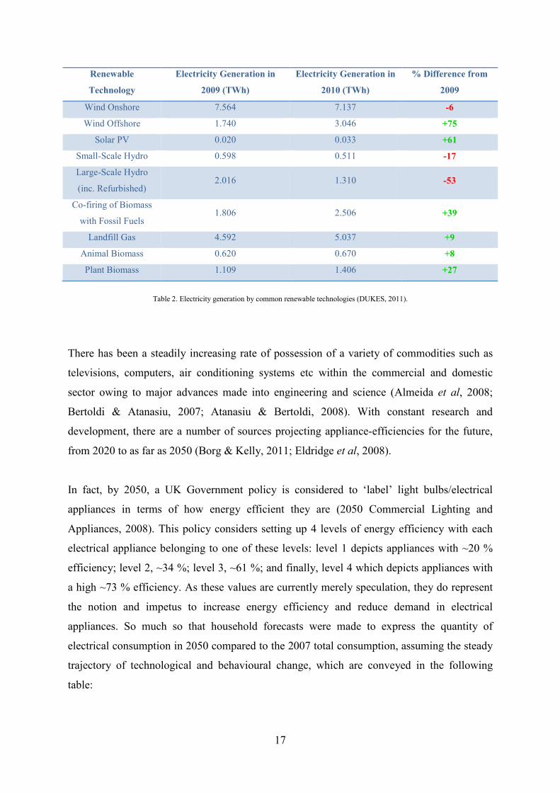
Table 2. Electricity generation by common renewable technologies (DUKES, 2011).

There has been a steadily increasing rate of possession of a variety of commodities such as

televisions, computers, air conditioning systems etc within the commercial and domestic

sector owing to major advances made into engineering and science (Almeida et al, 2008;

Bertoldi & Atanasiu, 2007; Atanasiu & Bertoldi, 2008). With constant research and

development, there are a number of sources projecting appliance-efficiencies for the future,

from 2020 to as far as 2050 (Borg & Kelly, 2011; Eldridge et al, 2008).

In fact, by 2050, a UK Government policy is considered to ‘label’ light bulbs/electrical

appliances in terms of how energy efficient they are (2050 Commercial Lighting and

Appliances, 2008). This policy considers setting up 4 levels of energy efficiency with each

electrical appliance belonging to one of these levels: level 1 depicts appliances with ~20 %

efficiency; level 2, ~34 %; level 3, ~61 %; and finally, level 4 which depicts appliances with

a high ~73 % efficiency. As these values are currently merely speculation, they do represent

the notion and impetus to increase energy efficiency and reduce demand in electrical

appliances. So much so that household forecasts were made to express the quantity of

electrical consumption in 2050 compared to the 2007 total consumption, assuming the steady

trajectory of technological and behavioural change, which are conveyed in the following

table:

18

2007 (TWh/y) 2050 – Level 1

(TWh/y)

2050 – Level 2

(TWh/y)

2050 – Level 3

(TWh/y)

2050 – Level 4

(TWh/y)

176 213 184 136 108

Table 3. Predicted electricity consumption for future scenarios (2050 Commercial Lighting and Appliances, 2008).

A clear and concise method to see the effects of energy-efficiency in appliances over a period

of time is to monitor and record the data. By doing so, annual sets of data can then be

compared and any changes witnessed. The database associated with this project can be

updated with such data for the same building over a number of years and graphs can be

shown to portray differences.

2.2 Renewable Heat

Renewable technologies play a significant role not only in electricity generation but also in

the production of heat (Nast et al, 2007). It was found that in the UK, approximately 16 % of

renewable sources were exploited to produce heat in 2010, amassing to a total of 1,212 ktoe

(kilo tonnes of oil equivalent). This is 17 % more than what was produced in 2009 and 103 %

more than in 2005 (DUKES, 2011).

Within the last few years, there has been a surge of renewable technologies being used to

generate heat after a period of decline which began more than a decade ago. The reason for

this was due to restrictions being placed on emission controls, which consequently

discouraged the onsite combustion of biomass (DUKES, 2011). Nowadays, the growth within

the domestic sector is primarily due to wood-burning (Lee et al, 2005); whereas plant

biomass has been widely used in the agricultural sector (Upreti & van der Horst, 2004). The

industrial sector are also consuming more wood than they did previously, which could be due

to financial reasons. Studies have shown that the consumption of wood has been the main

contributor in terms of renewable heat, this was found to ~32 % of the total heat produced by

renewable resources. The next 2 principal contributors, both of which summed up to 17 %

each, was the non-domestic use of wood and plant biomass (DUKES, 2011). The following

graph illustrates the input proportion of various renewable energy fuel-types:

Graph 3. Input of renewable energy f

For the first time in 2012, heat pumps (both air & ground sources) have been incorporated

into the DUKES statistics published by the Government

since 2008. It should be noted that only the net gain in energy (i.e. overall energy from heat

subtracted from the electricity used to operate the pump) is regarded as renewable energy

(DUKES, 2011). Unfortunately, heat pumps tend to use a

to power the compression cycles involved. Therefore, a Renewable Energy Directive was

drafted which considered proposing a method to surmise the possible amount of renewable

energy generated. This integrated a Seasonal

introduced in the performance of the heat pump if it is no longer considered in producing

energy from renewable means

for a heat pump to be considered

an SPF of 3 – this is the value assumed for all heat pumps set

(DUKES, 2011).

19

Input of renewable energy fuel-types in 2010 (DUKES, 2011).


into the DUKES statistics published by the Government – the data has



(DUKES, 2011). Unfortunately, heat pumps tend to use a considerable quantity of electricity



energy generated. This integrated a Seasonal Performance Factor (SPF) whereby a cut


energy from renewable means (Omer, 2008; Doherty et al, 2004). The minimum requirement

for a heat pump to be considered to generate renewable energy is for the technology to attain

this is the value assumed for all heat pumps set-up during 2008 and beyond


has been accumulated



considerable quantity of electricity



Performance Factor (SPF) whereby a cut-off is


. The minimum requirement

to generate renewable energy is for the technology to attain

up during 2008 and beyond

20

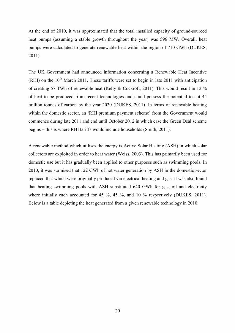
At the end of 2010, it was approximated that the total installed capacity of ground-sourced

heat pumps (assuming a stable growth throughout the year) was 596 MW. Overall, heat

pumps were calculated to generate renewable heat within the region of 710 GWh (DUKES,

2011).

The UK Government had announced information concerning a Renewable Heat Incentive

(RHI) on the 10th March 2011. These tariffs were set to begin in late 2011 with anticipation

of creating 57 TWh of renewable heat (Kelly & Cockroft, 2011). This would result in 12 %

of heat to be produced from recent technologies and could possess the potential to cut 44

million tonnes of carbon by the year 2020 (DUKES, 2011). In terms of renewable heating

within the domestic sector, an ‘RHI premium payment scheme’ from the Government would

commence during late 2011 and end until October 2012 in which case the Green Deal scheme

begins – this is where RHI tariffs would include households (Smith, 2011).

A renewable method which utilises the energy is Active Solar Heating (ASH) in which solar

collectors are exploited in order to heat water (Weiss, 2003). This has primarily been used for

domestic use but it has gradually been applied to other purposes such as swimming pools. In

2010, it was surmised that 122 GWh of hot water generation by ASH in the domestic sector

replaced that which were originally produced via electrical heating and gas. It was also found

that heating swimming pools with ASH substituted 640 GWh for gas, oil and electricity

where initially each accounted for 45 %, 45 %, and 10 % respectively (DUKES, 2011).

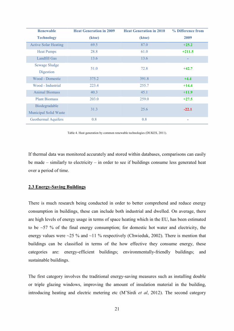
Below is a table depicting the heat generated from a given renewable technology in 2010:

21

Renewable

Technology

Heat Generation in 2009

(ktoe)

Heat Generation in 2010

(ktoe)

% Difference from

2009

Active Solar Heating 69.5 87.0 +25.2

Heat Pumps 28.8 61.0 +211.5

Landfill Gas 13.6 13.6 -

Sewage Sludge

Digestion 51.0 72.8 +42.7

Wood - Domestic 375.2 391.8 +4.4

Wood - Industrial 223.4 255.7 +14.4

Animal Biomass 40.3 45.1 +11.9

Plant Biomass 203.0 259.0 +27.5

Biodegradable

Municipal Solid Waste 31.3 25.6 -22.1

Geothermal Aquifers 0.8 0.8 -

Table 4. Heat generation by common renewable technologies (DUKES, 2011).

If thermal data was monitored accurately and stored within databases, comparisons can easily

be made – similarly to electricity – in order to see if buildings consume less generated heat

over a period of time.

2.3 Energy-Saving Buildings

There is much research being conducted in order to better comprehend and reduce energy

consumption in buildings, these can include both industrial and dwelled. On average, there

are high levels of energy usage in terms of space heating which in the EU, has been estimated

to be ~57 % of the final energy consumption; for domestic hot water and electricity, the

energy values were ~25 % and ~11 % respectively (Chwieduk, 2002). There is mention that

buildings can be classified in terms of the how effective they consume energy, these

categories are: energy-efficient buildings; environmentally-friendly buildings; and

sustainable buildings.

The first category involves the traditional energy-saving measures such as installing double

or triple glazing windows, improving the amount of insulation material in the building,

introducing heating and electric metering etc (M’Sirdi et al, 2012). The second category

22

focuses on the architecture of the building and how effective it stores/delivers energy. This

can include a building design which utilises passive solar as the main heat contributor,

underground thermal heating storage, and incorporating photovoltaic cells to name a few

methods (Yang et al, 2012). The final category concentrates on the protection of present and

future energy, water and land resources. Factors which can influence the mentioned resources

include the quality of the indoor environment, residential area and of building materials

(Hseih et al, 2011).

It is the aim of many organisations and Governments across the world to encourage and

convert all manner of buildings to those which can obtain the status of a ‘sustainable

building’. Studies have shown that the behaviours of those organisations can influence how

effective and efficient the level of energy-saving of buildings can be. This impact can be

hugely significant especially to businesses as Governments can offer grants depending on the

level of sustainability the business wishes to achieve (Xue & Li, 2011). These grants can also

be given to local housing schemes to aid consumers to invest in small-scale renewable energy

methods.

With current monitoring technologies which allows consumers to see extremely accurately

how much energy they are consuming, these monitoring devices can be applied to sustainable

buildings which could help achieve the best possible combination of technical, social,

economic and environmental factors. Sustainable buildings which boasts this type of

screening advancement are sometimes captioned ‘sustainable intelligent buildings’ and is

considered to be a significant part of a sustainable life cycle assessment (LCA) (Yu et al,

2011). The LCA is a method in which various aspects of a sustainable development are

measured (Guo et al, 2011). Some of these aspects include those which were mentioned

previously such as the amount of insulation in the building, efficient use of natural heating

and lighting etc. Different countries have differing policies and regulations, therefore the

LCA requirements can vary for buildings within these locations. If a building manages to

pass the LCA, then it can be considered to be a ‘sustainable building’ or a ‘sustainable

intelligent building’ if it is equipped with energy-reading devices.

23

2.4 SMART Buildings

A SMART building, or house, is one which has been installed with a particular system

consisting of hardware, software and wiring to allow the occupants to monitor and manage

the consumption of energy. This is accomplished by selecting which devices in the building

can be active at any given time by simply entering a single instruction when accessing the

systems network (Agarwal et al, 2010). This technology is seen as a major step in reducing

energy consumption – which in turn reduces carbon emissions.

SMART technology in buildings and dwellings are expanding swiftly along with electrical

technology with many buildings nowadays equipped with all manners of systems such as

security, entertainment, communication etc. Similar to electrical devices, there are a number

of SMART systems developed and deployed with similar and unique attributes. A typical

technology used is Powerline Carrier Systems (PCS) which involves the transmission of

encoded signals via the buildings electrical wiring network. These signals are delivered to

programmable switches which in turn are transmitted to specific devices – the signals contain

commands processed by the particular device (Yu-Ju et al, 2002).

A common procedure for PCS is a signalling method named X10, primarily used to

command electrical appliances connected to the network. The digital commands sent via X10

consist of shortwave radio-frequency pulses capable of allowing communication between

receivers and transmitters (Arora et al, 2002).

In Europe, collaboration between a number of countries had led to the creation of the

European Installation Bus (EIB) – or Instabus (Langhammer & Kays, 2011). This innovative

system utilised the use of a 2-wire bus line set up with the common electrical wiring network

and unites all connected electrical equipment to a decentralised communication mainframe.

The Instabus does not require an electrical switchboard or control console for operation,

instead a personal computer (PC) can be exploited to observe and ensure all appliances are

functioning correctly and at the scheduled time. These aspects of the Instabus aids in

decreasing power consumption and increasing comfort, security and building efficiency. In

fact, the association Konnex – which converged and improved the EIB and two other network

protocols – endeavours to regulate SMART building networks throughout Europe (Ruta et al,

2011).

24

A number of energy providers such as Scottish Power, Ofgem etc, are also developing and

improving SMART metering for consumers to see very precisely how much energy they are

using (Smart Meter Testing & Trialling Discussion Paper, 2011). This can help consumers to

manage their energy consumption much more efficiently, which provides them with the

added benefit better manage their energy costs. The SMART metering system is also

designed to let consumers know how much their monthly bill would be compared to

receiving estimated bills which would consequently cease meter-readers visiting homes. Due

to advantages of SMART metering, the UK Government hopes to have all households

installed with the meter by 2020 with the rollout of the device beginning this year

(Quantitative Research into Public Awareness, Attitudes, and Experience of Smart Meters,

2012). Although it is very beneficial and effective that SMART metering can monitor energy

consumption at high-resolution, it is unknown if any of the data monitored would be stored –

in which case, analysis of demand profiles could prove difficult.

2.5 Hybrid Renewable Energy Systems

A Hybrid Renewable Energy System integrates two or more combinations of energy-

conversion technologies in order to achieve greater system flexibility, efficiency and

productivity than an individual renewable energy device. There is a diverse range of Hybrid

Systems such as Biomass-Wind-Fuel Cell System, Photovoltaic-Wind System etc (Deshmukh

& Deshmukh, 2008). Although still in its early stages, many producers are opting to develop

low-costing Hybrid Renewable Energy Systems. This would aid in the global market’s

acceptance of such systems which in turn could provide substantial investment into research

and development (Burch, 2001).

These systems are designed to be highly resourceful by combining a selection of very

efficient technologies (such as fuel cells, progression in material-science etc). Energy storage

devices can also be used to improve reliability of a Hybrid Renewable Energy System if any

surplus energy has been generated (Rodolfo et al, 2008). Environmentally, these systems are

very capable in producing lower carbon-emissions than those systems which require fossil

fuels to operate (Ashok, 2007).

It is apparent that such systems are required, particularly since the Hybrid Systems operate

depending on environmental conditions. For example, installing Solar PV Panels in a region

25

in Scotland may provide a certain amount of energy but only if the intensity of sunlight

available is sufficient, otherwise the energy production is low. However, incorporating Wind

Turbines into the system alongside the Solar PV Panels can potentially generate much more

energy as Scotland receives a considerable amount of wind, particularly near the coast. Thus,

if there was little light present and an ample source of wind (or vice-versa), the Hybrid

Renewable Energy System could possess the ability to compensate for any limitations (Ekren

& Ekren, 2008).

Fortunately, there are DCMTs available which can analyse demand profiles with a collection

of different renewable technologies and hybrid systems: Merit is one such software which

will be used in this project.

2.6 Merit – Supply/Demand Energy Matching Tool

2.6.1 Overview

Developed by the ESRU department of the University of Strathclyde, Merit is a quantitative

evaluation software which enables the user to analyse the match between supply and demand

mechanisms and determine which combinations are the most suitable for a given scenario.

This analysing protocol processes various criterion such as matching the temporal demand of

the profile, reducing the required energy storage capacity and maximising the utilisation

factor of the renewable energy system. Within the simulation procedure, complex algorithms

exploit internal datasets, derived from weather/geographical sources and the producer’s

specifications, which are integrated to emulate physical practice. Merit can also provide the

option of recording the results in a high-resolution format such as half-hourly demand

profiles.

Although Merit can be used independently and offline, it does possess the capabilities of

exchanging data with several energy-analysing software over the internet. The type of data

communicated can range from simulated demand profiles from virtual building models to

weather conditions for a given geographical location. All these exchanges are accomplished

by the program connecting to a remote SQL (Structured Query Language) database.

26

2.6.2 Procedure

As Merit is a dynamic supply/demand matching-design tool for renewable energy systems, a

range of criteria must be entered depending on the user’s requirements. The analysis aims to

reach the highest possible temporal match between the combinations of both the supply and

demand factors - this establishes the successfulness of the combination when installed.

The procedural steps of using this supply/demand matching tool involve the user first

selecting the weather profile for their defined scenario. Next, the demand and renewable

supply profiles are chosen which form the significant prerequisite of the analysis. An

auxiliary or back-up system (battery, hot-water storage etc) can also be selected with

corresponding performance information displayed; a cost-indication of additional energy may

also be provided in the final analytical report as a function of a selected tariff. However, it is

not a compulsory option.

Once Merit collects the necessary input from the user-defined criterion, statistical techniques

are employed to analyse the supply and demand profiles. One of these techniques is based on

the Spearman’s Rank Correlation Coefficient which describes the trend between two

variables but does not take into account the relative magnitudes of the individual variables

(Scheaffer and McClave, 1982). The Correlation Coefficient, CC, results in a value which

will always lie between -1 and 1. When one variable increases towards 1 (perfect positive

correlation), the other variable decreases at exactly the same rate towards -1 (perfect negative

correlation). If CC = 0, then this would indicate that there is no correlation between the

variables.

The CC between supply and demand profiles in Merit is calculated by using Equation (1). If

the size of the supply profile was then increased in size (for example, twice as much), and the

demand profile remained the same, the CC would also remain the same regardless if the

surplus supply was greater. If, however, the supply and demand profiles possessed varying

quantities but were in perfect phase, the outcome would be a perfect correlation even though

the match would not be perfect. This technique gives a metric of potential matches which

could be possible if alterations are made, such as modifying the size of the renewable energy

system or increasing energy efficiency.

27

��

(1)

Where Dt = demand at time, t

St = supply at time, t

d = mean demand over time period, n

s = mean supply over time period, n

Another statistical technique used to analyse the match between supply and demand profiles

is based on an Inequality Coefficient described by Williamson and was primarily used to

confirm estimated thermal performance models (Williamson, 1994). The Inequality

Coefficient, IC (or Match Rate), expresses the difference of 3 variables in a time-series: the

unequal tendency (mean); the unequal variation (variance); and finally, the imperfect co-

variation (co-variance) (Born, 2001).

For Merit, the IC between supply and demand profiles is calculated by using Equation (2).

The IC results in a value which will always lie between 0 and 1. When IC = 0, the match is

perfect; when IC = 1, there is no match. Various matches due to inequalities can then be

termed by either ‘good matches’, particularly for those which range between 0 and 0.1; or

‘bad matches’ which range between 0.9 and 1 (Born, 2001).

��

(2)

This dynamic supply/demand matching method can be revised and replicated to study the

outcome of differing supply/demand parameters, time periods, weather data etc rapidly and

effortlessly.

28

Chapter 3: Collection, Collation and Interpolation of

Electrical/Thermal Demand Profiles

3.1 Collection and Collation of Demand Data

The majority of demand data collected for the purpose of this project was achieved by means

of contacting the necessary parties either by phone or email. In very few cases, the electrical

and thermal profiles were available for immediate download on dedicated websites. As

mentioned earlier, the origin of most of the data is based in Scotland; the remaining data are

located in England (excluding BAA Airport where the location will remain anonymous). All

profiles consist of annual data with a data resolution of half-hourly, hourly or monthly. The

following table shows obtained demand profiles for the type of building and the country they

are situated in:

Type of Building No. of Buildings

for Each Type

No. of Electrical

Demand Profiles

No. of Thermal Demand

Profiles Country Location

Care Home 7 7 3 Scotland

Community Centre 5 5 1 Scotland

Emergency Services 3 3 2 Scotland

Hall/Venue 3 3 1 Scotland

Houses: 2-Bed Mid-Terrace

2-Bed Semi-Detached

3-Bed Detached

3-Bed End-Terrace

3-Bed Semi-Detached

4-Bed Detached

5

24

12

6

14

18

5

24

12

6

14

18

5

24

6

-

6

18

England

England

England

England

England

England

High/Secondary School 24 24 4 Scotland

Leisure Centre 4 4 3 Scotland

Library 3 3 1 Scotland

Maintenance Services 5 5 - Scotland

Museum/Art Gallery 1 1 - Scotland

Nursery/Primary School 23 23 7 Scotland

Office 19 19 12 Scotland/England

Specialist School 5 5 - Scotland

Transport 4 4 - UK

University of Strathclyde 10 10 2 Scotland

Table 5. Type, no. of electrical/thermal and location of demand profiles for given building.

29

Although electrical demand data were acquired for ALL the buildings, only 32 % of the

buildings also possessed thermal (gas) demand data. In other words, with a combined total of

301 profiles collected: 206 are electrical; 95 are thermal. The profiles were all provided in a

Microsoft Excel format to allow data to be easily sorted, manipulated and edited if necessary.

While the profiles could still be used without the thermal consumption data, generating the

Generic profiles (which are discussed later) may have a reduction in accuracy if describing

thermal demand.

The main contributor to the data collected were various city councils such as Glasgow City

Council, Edinburgh City Council and so forth. Other sources included organisations such as

BAA, Building Research Establishment etc – all of whom are acknowledged. However, due

to the process of contacting the parties for the required information, the length of time in

which to receive the data in 80 % of the cases exceeded 3 weeks. This period of waiting for

the data could have been easily avoided had the data been made previously available online,

there would not have been any restrictions to the public accessing the data due to the

Freedom of Information Act 2000 and Freedom of Information (Scotland) Act 2002

(Legislation: Freedom of Information Act, 2000; Legislation: Freedom of Information

(Scotland) Act, 2002).

3.2 Interpolation of Demand Data

Once a profile was obtained, the data was thoroughly scrutinised to check the initial format of

the profile and to inspect for any obvious errors or missing data, in which case interpolation

techniques are employed.

3.2.1 Format of Data

The format of the collected demand profiles were important as they were to be tested in the

new supply/demand energy-matching software version of Merit. This tool requires profiles to

be in a comma-delimited format (.csv) and must not exceed 8,760 individual data cells for an

hourly resolution; 17,520 individual data cells for half-hourly resolution. The first 2 rows

must contain additional information of the data as shown in Figure 1: A1 – name of profile;

30

A2 – year of data; B2 and C2 – start and end day respectively; D2 – data resolution (1 =

hourly; 2 = half-hourly).

The data can then begin from A3 with each row representing a day and each column

representing an hour or half-hour. If hourly resolution data is used, the data for the first day

would start and end at A3 and X3 respectively (24 cells horizontally); for half-hourly

resolution, the data would start and end at A3 and AV3 respectively (48 cells horizontally).

Figure 1. Example of required format of demand profile.

31

3.2.2 Missing Individual Data Cells

It was found in a number of cases that there were missing individual pieces of data within the

profiles. An example can be seen below in Figure 2 which shows the format of a demand

profile – in this case, a Care Home in Scotland is illustrated with half-hourly data resolution.

The rows represent a day of the year; the columns represent the time in a half-hourly or

hourly period. For monthly data, all cells within the monthly duration of rows (i.e. 30 rows

for January; 28 for February etc) would be exactly the same. This level of accuracy is much

lower than that of a half-hourly or hourly resolution.

It must be noted that if the demand data contained few missing or inaccurate data – the source

will NOT be identified. This decision was made in order to protect the council/organisations’

credibility.

Figure 2. Example of a missing individual data cell.

32

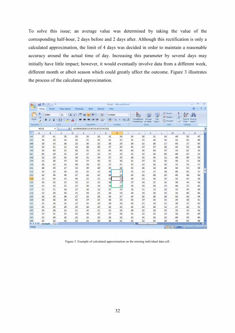
To solve this issue; an average value was determined by taking the value of the

corresponding half-hour, 2 days before and 2 days after. Although this rectification is only a

calculated approximation, the limit of 4 days was decided in order to maintain a reasonable

accuracy around the actual time of day. Increasing this parameter by several days may

initially have little impact; however, it would eventually involve data from a different week,

different month or albeit season which could greatly affect the outcome. Figure 3 illustrates

the process of the calculated approximation.

Figure 3. Example of calculated approximation on the missing individual data cell.

33

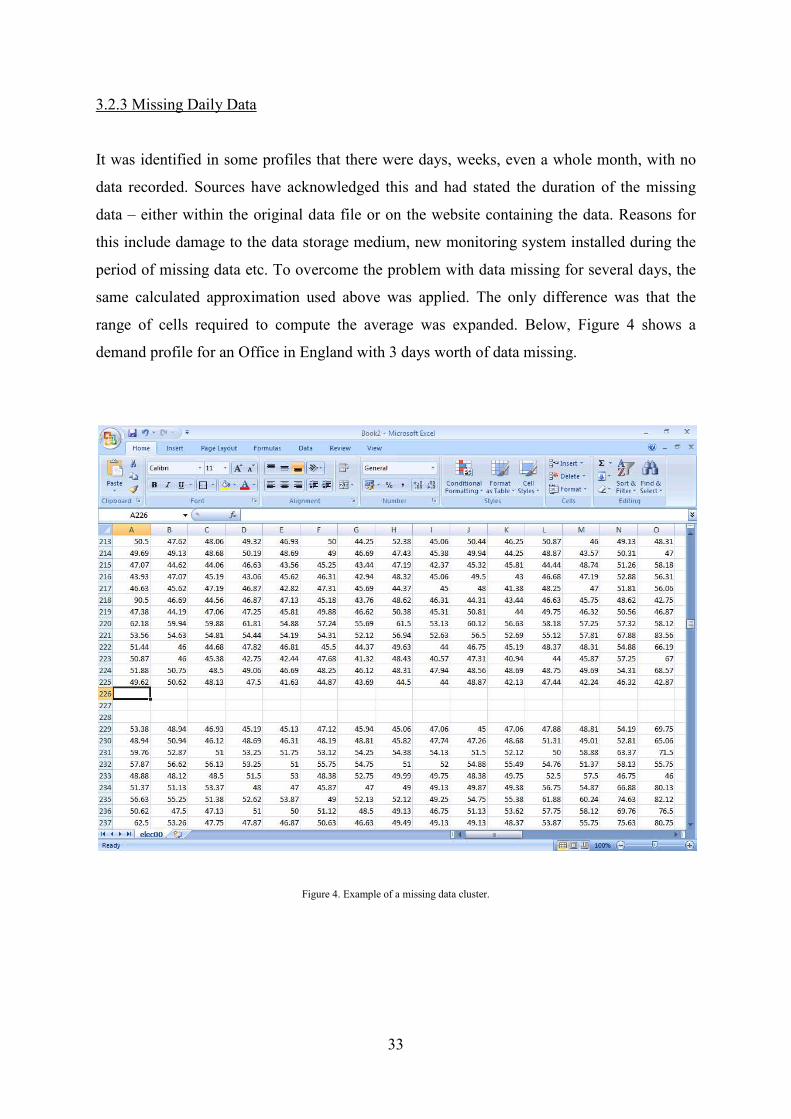
3.2.3 Missing Daily Data

It was identified in some profiles that there were days, weeks, even a whole month, with no

data recorded. Sources have acknowledged this and had stated the duration of the missing

data – either within the original data file or on the website containing the data. Reasons for

this include damage to the data storage medium, new monitoring system installed during the

period of missing data etc. To overcome the problem with data missing for several days, the

same calculated approximation used above was applied. The only difference was that the

range of cells required to compute the average was expanded. Below, Figure 4 shows a

demand profile for an Office in England with 3 days worth of data missing.

Figure 4. Example of a missing data cluster.

34

To resolve this issue, 2 data cells of the same hour but on 2 different days would be used to

estimate the individual missing cell. This can be seen more clearly in Figure 5 where the

coloured NUMBERS represent the result of the calculated approximation; the coloured

CELLS represent the data used to calculate the approximation. This process is then repeated

for the remaining missing cells.

The accuracy of this technique can be justified by explaining that those 3 days worth of data,

in a 365-days year, only accounts for 0.8 % of the annual data. Therefore, the accuracy of the

data for the missing 3 days can be viewed as insignificant – provided that the data is

reasonable and consistent with the data at the exact same time in the surrounding days.

Figure 5. Example of calculated approximation on the missing data cluster.

35

3.2.4 Missing Weekly/Monthly Data

Unfortunately, there were several demand profiles with data missing between 4 weeks and a

whole month – both of which accounts for 7.7 % and ~8.5 % respectively. These datasets

were originally collected by the Buildings Research Establishment (BRE) and describe the

hourly electrical and gas consumption rates of the houses which are examined in this project.

The reason for the missing data is due to damage to the storage medium. An example of the

problem is shown in Figure 6.

Figure 6. Example of missing weekly/monthly data.

36

No data is accessible for the month of April 1989; however, the original profile contained

data over a 2-3 year period. To resolve this problem, data from March 1989 and May 1989

were compared to March 1990 and May 1990 respectively. An average percentage difference

was calculated for each hour in March and May which was then applied to the hourly data in

April 1990. This provided a reasonable estimate to what the data would have been in April

1989 as shown in Figure 7.

Figure 7. Example of calculating the average percentage difference.

The calculated approximation of the data for April 1989 is then imported into the original

demand profile where the real data would have been. This process was applied to a small

number of demand profiles with several weeks of data missing.

37

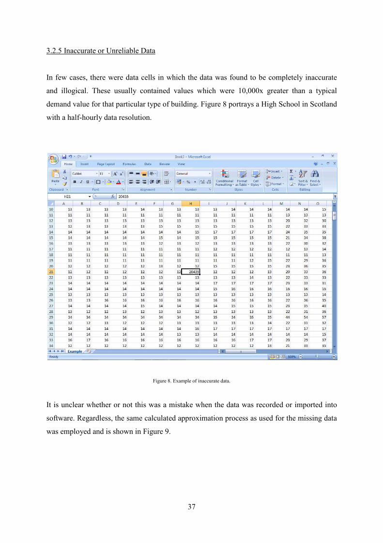
3.2.5 Inaccurate or Unreliable Data

In few cases, there were data cells in which the data was found to be completely inaccurate

and illogical. These usually contained values which were 10,000x greater than a typical

demand value for that particular type of building. Figure 8 portrays a High School in Scotland

with a half-hourly data resolution.

Figure 8. Example of inaccurate data.

It is unclear whether or not this was a mistake when the data was recorded or imported into

software. Regardless, the same calculated approximation process as used for the missing data

was employed and is shown in Figure 9.

38

Figure 9. Example of calculated approximation on inaccurate data.

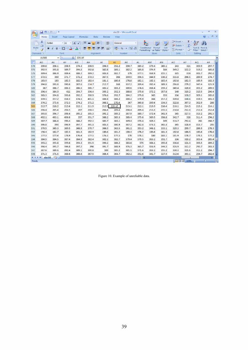
A small number of demand profiles also contained values which are considered defective.

Again the reasons for this are unclear. The sources of such profiles mention a similar

statement which basically reads the following: “numbers followed by an 'E' are unreliable

numbers”. Figure 10 shows a cell with unreliable data, this too is solved by conducting a

calculated approximation.

39

Figure 10. Example of unreliable data.

40

Chapter 4: Generic Demand Profile Generation

Once all the demand profiles were categorised, as shown in Chapter 3; Table 5, and refined,

further analysis was conducted to determine vital pieces of information for the particular

building. This included calculating and establishing the floor area, average daily occupancy,

annual energy consumption rate, annual energy consumption rate per floor area etc. The next

stage consisted of generating Generic Profiles – an electrical/thermal demand profile to

convey a typical profile for a given building type. For this, various pieces of data such as the

floor area, average daily occupancy, annual energy consumption per floor area etc were used

to calculate an overall average.

It should be noted that when constructing the Generic Profiles, not all of the demand profiles

were used for that particular building type. In order to achieve the highest accuracy possible

with the data provided, the annual electrical consumption per floor area (AECFA) was used

for Generic Profiling due to all buildings possessing electrical data. This was compared with

other profiles for the same type of building and those which had a relatively similar value

were utilised. However, the Generic Profile may also contain annual gas consumption per

floor area (AGCFA) data if the associated buildings contained sufficient thermal data. Both

Generic AECFA and Generic AGCFA were calculated by dividing the Generic annual

electric/gas consumption with the Generic floor area for each building type – another method

would have been to average the AECFA or AGCFA of the buildings to obtain a Generic

value, however, this was not done as the entire process would no longer be consistent.

The analysis of the demand profiles for the various types of buildings will now be discussed

in greater detail. Please note that only the information used for analysis and Generic Profiling

are displayed in this section. For more detailed information such as the year of build, the

councils which provided data, Energy Performance Certificate (EPC) or Display Energy

Certificate (DEC) ratings etc, please check the Profile Library (described in Chapter 5).

41

4.1 Care Home

Significant information for the 7 Care Homes, all of which were based in Scotland, is shown

in Table 6, these profiles were provided by 5 Scottish Councils. The period of the data in

which the demand profiles were recorded is 2011-2012. It is very clear that each Care Home

has differing floor areas and average daily occupancy, the results of which could have

considerable effects to energy consumption.

However, this is not always the case as can be seen with Bonnyton House Care Home from

East Renfrewshire and Muirpark Care Home from North Lanarkshire. Both of these

dwellings contain a floor area of 1,440 m2 and 1,416 m2 respectively; and an average daily

occupancy of 34 and 40 respectively. Although both these buildings are similar in these

respects, Bonnyton House consumes almost 4x more electricity (at 257,465 kWh/y) and 2x

more gas (at 802,174 kWh/y) than does Muirpark. This can be due to a number of reasons

such as the energy efficiency of the building, number and sophistication of equipment within

the building etc.

Building Annual Electrical

Consumption (kWh/y)

Annual Gas Consumption

(kWh/y)

Annual Electrical Consumption per

Floor Area (kWh/y/m2)

Annual Gas Consumption per


Floor Area (m2)

Average Daily

Occupancy

GENERIC CARE HOME

307,058.82 573,216.85 129.75 242.21 2,367 40

Bonnyton House Care

Home 257,464.56 802,173.98 178.79 557.07 1,440 34

Clermiston Care Home

735,664.00 - 294.03 - 2,502 36

Hillend House Care Home

230,023.60 - 379.58 - 606 50

Marrionville Court Care

Home 390,780.70 - 94.07 - 4,154 60

Muirpark Care Home

65,970.20 388,689.00 46.59 274.50 1,416 40

Silverlea Care Home

327,149.40 - 161.64 - 2,024 38

South Parks Care Home

146,336.11 528,787.56 85.43 308.69 1,713 32

Table 6. Care Home Data.

42

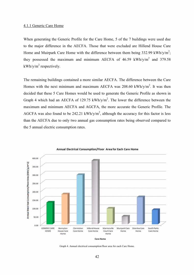
4.1.1 Generic Care Home

When generating the Generic Profile for the Care Home, 5 of the 7 buildings were used due

to the major difference in the AECFA. Those that were excluded are Hillend House Care

Home and Muirpark Care Home with the difference between them being 332.99 kWh/y/m2;

they possessed the maximum and minimum AECFA of 46.59 kWh/y/m2 and 379.58

kWh/y/m2 respectively.

The remaining buildings contained a more similar AECFA. The difference between the Care

Homes with the next minimum and maximum AECFA was 208.60 kWh/y/m2. It was then

decided that these 5 Care Homes would be used to generate the Generic Profile as shown in

Graph 4 which had an AECFA of 129.75 kWh/y/m2. The lower the difference between the

maximum and minimum AECFA and AGCFA, the more accurate the Generic Profile. The

AGCFA was also found to be 242.21 kWh/y/m2, although the accuracy for this factor is less

than the AECFA due to only two annual gas consumption rates being observed compared to

the 5 annual electric consumption rates.

Graph 4. Annual electrical consumption/floor area for each Care Home.

43

4.2 Community Centre

Five Community Centres were analysed, all of which were based in Scotland and provided by

3 Scottish Councils, the period in which these demand profiles were recorded was 2011-

2012. Table 7 shows various pieces of important information concerning the Community

Centres such as their corresponding floor areas: this varies greatly – from 272 m2 for the

Albertslund Community Centre to 1,885 m2 for the Inch Community Education Centre.

Unfortunately, the only annual gas consumption value recorded for these buildings was

54,000 kWh for the Albertslund Community Centre. This also held the lowest annual

consumption rate for electricity which was 5,948 kWh/y compared to the highest value of

140,710 kWh/y held by Inch Community Education Centre.

Building

Annual Electrical

Consumption (kWh/y)


(kWh/y)





Floor Area (m2)

Average Daily

Occupancy

GENERIC COMMUNITY

CENTRE 69,171.84 - 65.53 - 1,056 97

Albertslund Community

Centre 5,948.00 54,000.00 21.87 198.53 272 80

Burdiehouse Community

Centre 81,341.30 - 77.47 - 1,050 80

Cameron House Community

Centre 44,580.70 - 37.43 - 1,191 150

Garrel Vale Community

Centre 72,318.40 - 82.18 - 880 100

Inch Community Education

Centre

140,709.60 - 74.65 - 1,885 75

Table 7. Community Centre Data.

44

4.2.1 Generic Community Centre

Producing the Generic Profiles for the Community Centres involved all 5 of the buildings due

to the slight contrast of the AECFA. These would have little effect in reducing the overall

accuracy. These 5 Centres utilised a very similar amount of electrical energy per floor area

which contains a difference between the maximum and minimum of 60.31 kWh/y/m2.

The Generic Profile as shown in Graph 5 was calculated to have an AECFA of 65.53

kWh/y/m2.

Graph 5. Annual electrical consumption/floor area for each community centre.

45

4.3 Emergency Services

Demand profiles were obtained for only 3 Emergency Services, each one depicting a different

service building: Fire, Hospital and Police. The data was based from April 2011 to March

2012. These buildings are situated in various parts of Scotland, all of which containing

varying degrees of information as shown in Table 8. The floor area for Glasgow Royal

Infirmary is 84x and 56x greater than the Fire Station and Police Station respectively. In

terms of annual electrical consumption, the Hospital consumes 85x and 50x more than the

Fire and Police stations respectively. It is interesting to note that although the range of factors

is diverse; their AECFA is relatively similar – from 116.99 kWh/y/m2 for the Fire Station, to

118.81 kWh/y/m2 for Glasgow Royal Infirmary, and finally 133.54 kWh/y/m2 for the Police

Station.


Consumption (kWh/y)


(kWh/y)





Floor Area (m2)

Average Daily

Occupancy

Fire Station

278,323.00 382,842.00 116.99 160.93 2,379 76

Glasgow Royal

Infirmary 23,714,156.00 - 118.81 - 199,600 918

Police Station

476,990.00 908,208.00 133.54 254.26 3,572 253

Table 8. Emergency Services Data.

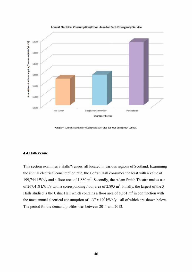
4.3.1 Generic Emergency Services

Due to the dissimilar type of Emergency Services, no Generic Profile could be made.

Nevertheless, the demand profiles for these buildings were analysed and Graph 6 illustrates

their respective AECFA.

46

Graph 6. Annual electrical consumption/floor area for each emergency service.

4.4 Hall/Venue

This section examines 3 Halls/Venues, all located in various regions of Scotland. Examining

the annual electrical consumption rate, the Corran Hall consumes the least with a value of

199,744 kWh/y and a floor area of 1,880 m2. Secondly, the Adam Smith Theatre makes use

of 267,418 kWh/y with a corresponding floor area of 2,895 m2. Finally, the largest of the 3

Halls studied is the Ushar Hall which contains a floor area of 8,861 m2 in conjunction with

the most annual electrical consumption of 1.37 x 106 kWh/y – all of which are shown below.

The period for the demand profiles was between 2011 and 2012.

47


Consumption (kWh/y)


(kWh/y)





Floor Area (m2)

Average Daily

Occupancy

GENERIC HALL

613,066.09 - 134.88 - 4,545 858

Adam Smith

Theatre 267,417.86 629,891.66 92.37 217.58 2,895 475

Corran Hall

199,744.40 - 106.25 - 1,880 600

Ushar Hall 1,371,909.80 - 154.83 - 8,861 1,500

Table 9. Hall/Venue Data.

4.4.1 Generic Hall/Venue

The Generic Profiles generated for the Hall/Venue consisted of using all 3 of the buildings as

there were no major distinctions in the AECFA. The difference between the maximum and

minimum values of the AECFA is 62.46 kWh/y/m2. The Generic Profile was computed to

have an AECFA rate of 134.88 kWh/y/m2 and is shown in Graph 7.

Graph 7. Annual electrical consumption/floor area for each Hall/Venue.

48

4.5 High/Secondary School

A large number of demand profiles for 24 High Schools (from 2011 to 2012) were obtained,

all based in Scotland with most located in Edinburgh. Although there is a large variety of data

provided, there are also similarities between several schools for numerous factors such as

AECFA and floor area. These schools range from smaller schools such as Tiree School, with

a 2,160 m2 floor area and average daily occupancy of 83, to a much larger school such as

Forrester & St Augustines High School, with a 27,865 m2 floor area and average daily

occupancy of 1,352. The annual electrical consumption rates also vary from as little as

56,090 kWh/y (Mearns Academy) to as much as 1.7 x 106 kWh/y (Forrester & St Augustines

High School). Table 10 does not provide the complete list of schools but it does quite clearly

show that buildings with a larger floor area do not necessarily consume more energy than

those with a smaller floor area (Broughton High School and Ellon Academy are two such

examples).


Consumption (kWh/y)


(kWh/y)

Annual Electrical Consumption per Floor

Area (kWh/y/m2)

Annual Gas Consumption per Floor

Area (kWh/y/m2)

Floor Area (m2)

Average Daily

Occupancy (LOW) GENERIC HIGH SCHOOL

393,956.19 - 35.13 - 11,215 742

Currie High School

526,484.70 - 43.27 - 12,167 921

James Gillespie's High

School 492,974.80 - 43.13 - 11,430 1,129

Liberton High School

446,282.50 - 33.95 - 13,145 697

Mearns Academy

56,090.10 1,710.93 7.42 0.23 7,562 603

(MEDIUM) GENERIC HIGH

SCHOOL 709,971.84 - 52.56 - 13,508 983

Broughton High School

974,471.70 - 53.91 - 18,076 895

Portobello High School

702,475.70 - 45.71 - 15,368 1,421

South Queensferry High School

562,916.00 - 48.80 - 11,535 786

Trinity Academy

554,530.40 - 47.23 - 11,742 905

(HIGH) GENERIC HIGH SCHOOL

996,083.60 - 71.08 - 14,014 747

Ellon Academy 1,225,027.60 38,686.08 74.15 2.34 16,520 1,061

Forrester & St Augustines High School

1,732,354.20 - 62.17 - 27,865 1,352

Tiree School 399,164.60 - 184.80 - 2,160 83

Tynecastle High School

825,032.40 - 63.06 - 13,084 576

Table 10. High/Secondary School Data.

49

4.5.1 Generic High/Secondary School

As a result of this many profiles and a vast range of data (regarding consumption rates, floor

areas and average daily occupancy), it was decided to categorise the schools in terms of the

AECFA in order to produce an effective and accurate Generic Profile. Therefore, 3 groups of

High Schools, each containing 8 schools, were created. To clarify: all schools are sorted from

largest to smallest in terms of their AECFA; the first 8 schools would be brought together to

create a HIGH Group; the next 8 schools would represent the MEDIUM Group; finally, the

remaining 8 with the lowest AECFA would depict the LOW Group.

As a result, 3 Generic Profiles were produced and shown below with their associated Group.

The LOW, MEDIUM and HIGH Groups have an AECFA of 35.13 kWh/y/m2, 52.56

kWh/y/m2 and 71.08 kWh/y/m2 respectively.

Graph 8. (LOW) annual electrical consumption/floor area for each High School.

50

Graph 9. (MEDIUM) annual electrical consumption/floor area for each High School.

Graph 10. (HIGH) annual electrical consumption/floor area for each High School.

51

4.6 Houses

Demand profiles for an assortment of 79 houses were scrutinised and classified according to

their type, some of which are tabulated below. The data for these houses were part of the

‘Milton Keynes Energy Park Dwellings 1990’, originally collected by the Building Research

Establishment (BRE) and provided by the UK Energy Research Centre. These dwellings

were constructed with the aim to be highly energy efficient. The name of each individual

house contains the letters ‘MK’ followed by a set of numbers to distinguish it from the other

houses.

Those of a particular dwelling-type consisting of (A) and (B) were further classed according

to their structural characteristics such as the depth of floor insulation, the U-Value of the

floor, roof, external walls etc. These characteristics can be fully viewed in the Profile Library.

The period of the data selected was based between 1989 and 1990. Although the data is

somewhat outdated, the process of analysis and Generic Profiling would still apply to data of

any period.

52

Dwelling Type

Annual Electrical Consumption

(kWh/y)


(kWh/y)

Annual Electrical Consumption per Floor

Area (kWh/y/m2)

Annual Gas Consumption per Floor Area

(kWh/y/m2)

Floor Area (m2)

Maximum Occupancy

2-BED MID-TERRACE:

MK0822 1,572.19 9,114.80 26.07 151.16 60.3 4

MK0825 3,042.76 10,533.98 50.46 174.69 60.3 4

2-BED SEMI-DETACHED

(A):

MK0819 43,475.65 8,537.97 692.29 135.95 62.8 4

MK0820 3,335.11 12,864.18 53.11 204.84 62.8 4

2-BED SEMI-DETACHED

(B):

MK0805 1,928.19 13,449.86 29.76 207.56 64.8 4

MK0811 1,261.23 4,255.10 19.46 65.67 64.8 4

3-BED

DETACHED (A):

MK0883 5,567.86 18,267.14 73.07 239.73 76.2 5

MK0884 2,731.97 9,451.13 35.85 124.03 76.2 5

3-BED

DETACHED (B):

MK0750 14,275.69 - 136.48 - 104.6 5

MK0754 14,278.38 - 136.50 - 104.6 5

3-BED END-TERRACE:

MK0751 6,705.16 - 84.45 - 79.4 5

MK0753 7,830.90 - 98.63 - 79.4 5

3-BED SEMI-DETACHED

(A):

MK0802 2,971.62 10,514.14 39.99 141.51 74.3 5

MK0803 3,407.42 11,993.75 45.86 161.42 74.3 5

3-BED SEMI-DETACHED

(B):

MK0758 7,553.87 - 86.43 - 87.4 5

MK0761 12,195.08 - 139.53 - 87.4 5

4-BED

DETACHED:

MK0890 6,519.37 19,413.77 46.87 139.57 139.1 6

MK0892 4,562.85 13,016.17 32.80 93.57 139.1 6

Table 11. House Data.

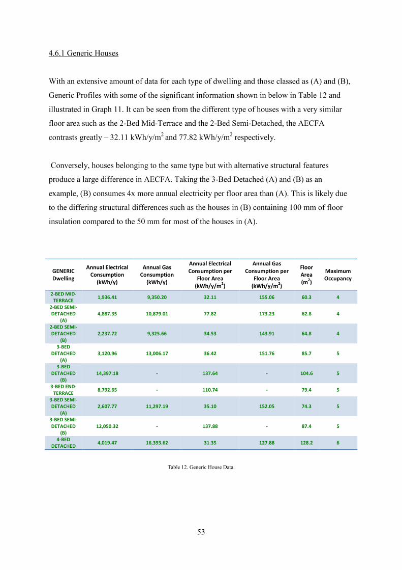
53

4.6.1 Generic Houses

With an extensive amount of data for each type of dwelling and those classed as (A) and (B),

Generic Profiles with some of the significant information shown in below in Table 12 and

illustrated in Graph 11. It can be seen from the different type of houses with a very similar

floor area such as the 2-Bed Mid-Terrace and the 2-Bed Semi-Detached, the AECFA

contrasts greatly – 32.11 kWh/y/m2 and 77.82 kWh/y/m2 respectively.

Conversely, houses belonging to the same type but with alternative structural features

produce a large difference in AECFA. Taking the 3-Bed Detached (A) and (B) as an

example, (B) consumes 4x more annual electricity per floor area than (A). This is likely due

to the differing structural differences such as the houses in (B) containing 100 mm of floor

insulation compared to the 50 mm for most of the houses in (A).

GENERIC Dwelling

Annual Electrical Consumption

(kWh/y)


(kWh/y)





Floor Area (m2)

Maximum Occupancy

2-BED MID-TERRACE

1,936.41 9,350.20 32.11 155.06 60.3 4

2-BED SEMI-DETACHED

(A) 4,887.35 10,879.01 77.82 173.23 62.8 4

2-BED SEMI-DETACHED

(B) 2,237.72 9,325.66 34.53 143.91 64.8 4

3-BED DETACHED

(A) 3,120.96 13,006.17 36.42 151.76 85.7 5

3-BED DETACHED

(B) 14,397.18 - 137.64 - 104.6 5

3-BED END-TERRACE

8,792.65 - 110.74 - 79.4 5

3-BED SEMI-DETACHED

(A) 2,607.77 11,297.19 35.10 152.05 74.3 5

3-BED SEMI-DETACHED

(B) 12,050.32 - 137.88 - 87.4 5

4-BED DETACHED

4,019.47 16,393.62 31.35 127.88 128.2 6

Table 12. Generic House Data.

54

Graph 11. Generic annual electrical consumption/floor area for each dwelling-type.

4.7 Leisure Centre

Profiles for four Leisure Centres were provided by 4 Scottish Councils, all of which are

between 2011 and 2012. There are discrepancies in terms of the annual electrical

consumption with Barrhead Leisure Centre making use of 805,844 kWh/y and an AECFA of

160.82 kWh/y/m2 compared to a Leisure Centre from the Angus region which annually

consumes 233,161 kWh/y with an AECFA of 66.94 kWh/y/m2.

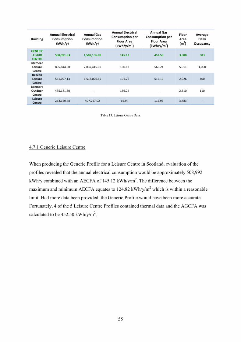
55


Consumption (kWh/y)


(kWh/y)





Floor Area (m2)

Average Daily

Occupancy

GENERIC LEISURE CENTRE

508,991.93 1,587,156.08 145.12 452.50 3,508 503

Barrhead Leisure Centre

805,844.00 2,837,415.00 160.82 566.24 5,011 1,000

Beacon Leisure Centre

561,097.13 1,513,026.65 191.76 517.10 2,926 400

Benmore Outdoor Centre

435,181.50 - 166.74 - 2,610 110

Leisure Centre

233,160.78 407,257.02 66.94 116.93 3,483 -

Table 13. Leisure Centre Data.

4.7.1 Generic Leisure Centre

When producing the Generic Profile for a Leisure Centre in Scotland, evaluation of the

profiles revealed that the annual electrical consumption would be approximately 508,992

kWh/y combined with an AECFA of 145.12 kWh/y/m2. The difference between the

maximum and minimum AECFA equates to 124.82 kWh/y/m2 which is within a reasonable

limit. Had more data been provided, the Generic Profile would have been more accurate.

Fortunately, 4 of the 5 Leisure Centre Profiles contained thermal data and the AGCFA was

calculated to be 452.50 kWh/y/m2.

56

Graph 12. Annual electrical consumption/floor area for each Leisure Centre.

4.8 Library

Data from only 3 Scottish Libraries were obtained and evaluated. The period for these

demand profiles was 2011. By far the largest of the 3 libraries is the Edinburgh Central

Library which encompasses a floor area of 6,500 m2; Glenwood Library and a library from

Angus both possessed a floor area of 349 m2 and 827 m2 respectively. Edinburgh Central

Library also consumes the most electricity annually at 366, 412 kWh/y compared to only

44,623 kWh/y for Glenwood Library. Interestingly, the smallest Library, Glenwood, has the

highest AECFA (127.86 kWh/y/m2) with the largest Library, Edinburgh Central, having the

lowest (56.37 kWh/y/m2).

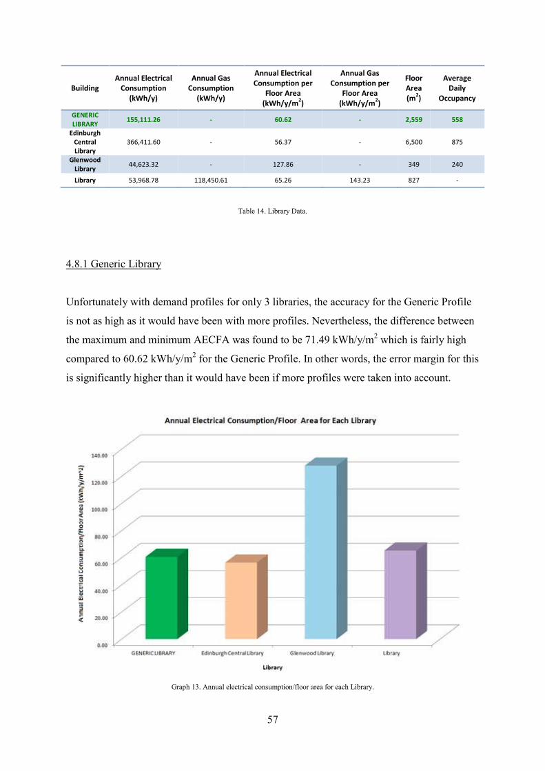
57


Consumption (kWh/y)


(kWh/y)





Floor Area (m2)

Average Daily

Occupancy

GENERIC LIBRARY

155,111.26 - 60.62 - 2,559 558

Edinburgh Central Library

366,411.60 - 56.37 - 6,500 875

Glenwood Library

44,623.32 - 127.86 - 349 240

Library 53,968.78 118,450.61 65.26 143.23 827 -

Table 14. Library Data.

4.8.1 Generic Library

Unfortunately with demand profiles for only 3 libraries, the accuracy for the Generic Profile

is not as high as it would have been with more profiles. Nevertheless, the difference between

the maximum and minimum AECFA was found to be 71.49 kWh/y/m2 which is fairly high

compared to 60.62 kWh/y/m2 for the Generic Profile. In other words, the error margin for this

is significantly higher than it would have been if more profiles were taken into account.

Graph 13. Annual electrical consumption/floor area for each Library.

58

4.9 Maintenance Services

These buildings incorporate a range of equipment and building maintenance services

alongside a number of depots. These were situated in Edinburgh with varying annual

electrical consumption rates: from a low 0.19 x 106 kWh/y for the Community Equipment

Services to as high as 1.06 x 106 kWh/y. No thermal or average daily occupancy data were

available for analysis, the demand profiles were all based in 2011. The AECFA also ranges

from as little as 42.94 kWh/y/m2 (Sighthill Roads Depot) compared to 230.47 kWh/y/m2

(Powerderhall Depot), more than 5x difference.

Building

Annual Electrical

Consumption (kWh/y)


(kWh/y)





Floor Area (m2)

Average Daily

Occupancy

Community Equipment

Services 189,938.00 - 64.74 - 2,934 -

Edinburgh Building Services

725,032.30 - 68.70 - 10,553 -

Powerderhall Depot

1,062,922.40 - 230.47 - 4,612 -

Russel Road Depot

530,520.60 - - - - -

Sighthill Roads Depot

294,630.80 - 42.94 - 6,861 -

Table 15. Maintenance Services Data.

4.9.1 Generic Maintenance Services

Due to the dissimilar type of Maintenance Services, no Generic Profile could be made.

Nevertheless, the demand profiles for these buildings were analysed and Graph 14 illustrates

their respective AECFA.

59

Graph 14. Annual electrical consumption/floor area for each Maintenance Service.

4.10 Museum/Art Gallery

Edinburgh City Council provided the only demand profile (electrical) for this type of

building. The City Arts Centre, encompassing 2,584 m2 consumed 506,632 kWh/y in 2011

with an AECFA of 196.07 kWh/y/m2.


Consumption (kWh/y)


(kWh/y)





Floor Area (m2)

Average Daily

Occupancy

City Arts Centre

506,632.00 - 196.07 - 2,584 -

Table 16. Museum/Art Gallery Data.

60

4.10.1 Generic Museum/Art Gallery

With only one demand profile, it was not possible to create a Generic Profile for this type of

building.

4.11 Nursery/Primary School

A large number of demand profiles for 22 Nursery/Primary Schools (from 2011 to 2012)

were obtained, all based in Scotland with most located in Edinburgh. With a large quantity of

statistics, similarities were distinguished in terms of AECFA. These schools range from a

small floor area of 615 m2 (Pikeman Nursery) to a large floor area of 6,980 m2 (Niddrie/St

Francis Primary School).

The Niddrie/St Francis Primary School is an example of a joint campus in which both nursery

and primary school students attend. It should be noted that both Carricknowe Nursery and

Carricknowe Primary are part of the same building and only the Nursery is shown in Table

17. The statistics for both these Schools in the Profile Library are shown to be exactly the

same due to the summation of data, however, their individual demand profiles differ greatly.

The annual electrical consumption rates also vary from as little as 36,531 kWh/y (Pikeman

Nursery) to as much as 532,080 kWh/y (Blackfriars Primary School). It can be seen from

Table 17, which does not show the complete list of schools, that a Nursery/Primary School

with larger floor area does not necessarily consume more energy than those with a smaller

floor area (Ashpark Primary School and Gylemuir Primary School are an example).

61


Consumption (kWh/y)


(kWh/y)




(kWh/y/m2)

Floor Area (m2)

Average Daily

Occupancy

(LOW) GENERIC NURSERY/PRIMARY

SCHOOL

79,921.19 499,826.63 24.45 152.93 3,268 395

Carolside Primary School

202,890.00 845,619.00 35.08 146.22 5,783 751

Crookfur Primary School

85,140.00 469,816.00 36.56 201.72 2,329 246

Gylemuir Primary School

141,959.50 - 35.48 - 4,001 383

St Joseph's Primary School

94,905.00 372,240.00 40.40 158.47 2,349 357

(MEDIUM) GENERIC NURSERY/PRIMARY

SCHOOL

169,714.82 - 44.65 - 3,801 422

Canal View Primary School

159,621.80 - 44.88 - 3,557 229

Carricknowe Nursery 208,222.20 - 49.04 - 4,246 504

Mearns Primary School

311,572.00 828,826.00 49.64 132.06 6,276 808

Pentland Primary School

166,057.70 - 46.09 - 3,603 330

(HIGH) GENERIC NURSERY/PRIMARY

SCHOOL

295,853.59 - 106.28 - 2,784 275

Ashpark Primary School

270,007.70 - 90.00 - 3,000 287

Blackfriars Primary School

532,080.10 - 224.51 - 2,370 225

Niddrie/St Francis Primary School

387,233.20 - 55.48 - 6,980 780

Parsons Primary School

422,628.00 - 168.04 - 2,515 288

Pikeman Nursery 36,531.10 - 59.40 - 615 115

Table 17. Nursery/Primary School Data.

4.11.1 Generic Nursery/Primary School

As a result of the number of profiles and a wide range of data (concerning consumption rates,

floor areas, average daily occupancy etc), it was decided to utilise the same Generic process

as conducted with High/Secondary Schools. Therefore, the Nursery/Primary Schools were

categorised in terms of their AECFA in order to produce 3 effective and accurate Generic

Profiles: LOW, MEDIUM and HIGH.

62

The LOW, MEDIUM and HIGH groups contain 7, 8 and 7 Nursery/Primary Schools

respectively according to their AECFA rate of 24.45 kWh/y/m2, 44.65 kWh/y/m2 and 106.28

kWh/y/m2 respectively. The LOW group also contained thermal data – 6 of the 7 schools – in

which it was possible to calculate the AGCFA, this was found to be 152.93 kWh/y/m2.

Graph 15. (LOW) annual electrical consumption/floor area for each Nursery/Primary School.

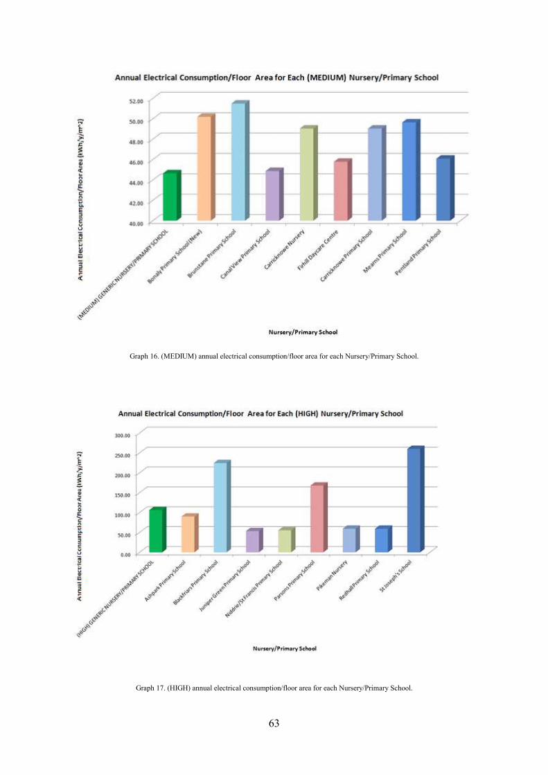
63

Graph 16. (MEDIUM) annual electrical consumption/floor area for each Nursery/Primary School.

Graph 17. (HIGH) annual electrical consumption/floor area for each Nursery/Primary School.

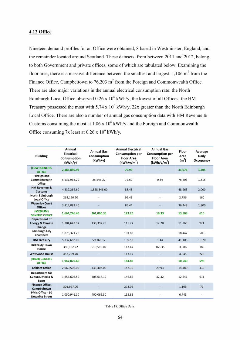
64

4.12 Office

Nineteen demand profiles for an Office were obtained, 8 based in Westminster, England, and

the remainder located around Scotland. These datasets, from between 2011 and 2012, belong

to both Government and private offices, some of which are tabulated below. Examining the

floor area, there is a massive difference between the smallest and largest: 1,106 m2 from the

Finance Office, Campbeltown to 76,203 m2 from the Foreign and Commonwealth Office.

There are also major variations in the annual electrical consumption rate: the North

Edinburgh Local Office observed 0.26 x 106 kWh/y, the lowest of all Offices; the HM

Treasury possessed the most with 5.74 x 106 kWh/y, 22x greater than the North Edinburgh

Local Office. There are also a number of annual gas consumption data with HM Revenue &

Customs consuming the most at 1.86 x 106 kWh/y and the Foreign and Commonwealth

Office consuming 7x least at 0.26 x 106 kWh/y.

Building

Annual Electrical

Consumption (kWh/y)


(kWh/y)





Floor Area (m2)

Average Daily

Occupancy

(LOW) GENERIC OFFICE

2,485,850.92 - 79.99 - 31,076 1,205

Foreign and Commonwealth

Office 5,531,964.20 25,545.27 72.60 0.34 76,203 1,815

HM Revenue & Customs

4,332,264.60 1,858,346.00 88.48 - 48,965 2,000

North Edinburgh Local Office

263,156.20 - 95.48 - 2,756 160

Waverley Court Offices

3,114,083.40 - 85.44 - 36,448 1,800

(MEDIUM) GENERIC OFFICE

1,664,246.40 261,060.30 123.25 19.33 13,503 616

Department of Energy & Climate

Change 1,304,643.97 138,397.29 115.77 12.28 11,269 924

Edinburgh City Chambers

1,878,321.20 - 101.82 - 18,447 500

HM Treasury 5,737,682.00 59,168.17 139.58 1.44 41,106 1,670

Kirkcaldy Town House

350,182.22 519,519.02 113.47 168.35 3,086 180

Westwood House 457,759.70 - 113.17 - 4,045 220

(HIGH) GENERIC OFFICE

1,947,870.60 - 184.82 - 10,540 598

Cabinet Office 2,060,506.00 433,403.00 142.30 29.93 14,480 430

Department for Culture, Media &

Sport 1,856,606.50 408,618.19 146.87 32.32 12,641 611

Finance Office, Campbeltown

301,997.00 - 273.05 - 1,106 71

PM's Office - 10 Downing Street

1,050,946.10 400,069.30 155.81 - 6,745 -

Table 18. Office Data.

65

4.12.1 Generic Office

As 19 demand profiles were collected, the same Generic Process used for High/Secondary

Schools and Nursery/Primary Schools was applied for Offices. The 3 Generic groups – LOW,

MEDIUM and HIGH – all contained 6, 7 and 6 Offices respectively and were sorted by their

AECFA. The LOW group boasted an AECFA of 79.99 kWh/y/m2; 123.25 kWh/y/m2 for

MEDIUM; and 184.82 for HIGH.

Surprisingly, when scrutinising the floor area for the Generic Profiles, the LOW group with

the lowest AECFA was calculated to have the highest floor area at 31, 076 m2; MEDIUM had

a median floor area 13, 503 m2; HIGH was computed to have the lowest floor area of 10,540

m2.

Graph 18. (LOW) annual electrical consumption/floor area for each Office.

66

Graph 19. (MEDIUM) annual electrical consumption/floor area for each Office.

Graph 20. (HIGH) annual electrical consumption/floor area for each Office.

67

4.13 Specialist School

Based in Edinburgh, 5 Specialist Schools were investigated and their corresponding data

from 2011 is shown in Table 19. No thermal data were available; however, the annual

electrical consumption rates vary from the lowest of 136,097 kWh/y (Woodlands School) to

as high as 298,716 kWh/y (Oaklands Special School).


Consumption (kWh/y)


(kWh/y)





Floor Area (m2)

Average Daily

Occupancy

GENERIC SPECIALIST

SCHOOL 182,077.58 - 69.65 - 2,614 65

Gorgie Mills School

164,542.30 - 59.70 - 2,756 54

Kaimes Special School

145,748.30 - 49.97 - 2,917 98

Oaklands Special School

298,716.30 - 81.00 - 3,688 44

St Crispins Special School

164,150.30 - 116.83 - 1,405 50

Woodlands School

136,097.70 - 59.07 - 2,304 78

Table 19. Specialist School Data.

4.13.1 Generic Specialist School

A Generic Profile was created by exploiting the datasets for all 5 Specialist Schools. It was

determined that the difference between the minimum and maximum AECFA was 66.86

kWh/y/m2; the minimum of 49.97 kWh/y/m2 belonging to Kaimes Special School and the

maximum of 116.83 kWh/y/m2 belonging to St Crispins Special School. The Generic annual

electrical consumption was then found to be 182,078 kWh/y with an AECFA of 69.65

kWh/y/m2 as exemplified below in Graph 21.

68

Graph 21. Annual electrical consumption/floor area for each Specialist School.

4.14 Transport

Demand profiles were obtained for 2 different types of Transport buildings: a BAA Airport

based in the UK (which will not be identified), and a Bus Station sited in Edinburgh. Only the

electrical consumption rate and floor area for both these buildings were obtained – however,

3 years worth of data for the BAA Airport was included, from 2009 to 2011, which clearly

shows a constant reduction in annual electrical consumption and AECFA. The main cause for

this may be due to improved energy efficiency methods employed within the Airport and

increased investment in renewable technologies such as Solar PV Panels.

69

Building Period

of Data

Annual Electrical

Consumption (kWh/y)


(kWh/y)




(kWh/y/m2)

Floor Area (m2)

Average Daily

Occupancy

BAA Airport

2009 32,410,265.20 - 595.99 - 54,381 -

BAA Airport

2010 31,205,064.50 - 573.82 - 54,381 -

BAA Airport

2011 30,039,622.20 - 552.39 - 54,381 -

Bus Station (New)

2011 836,816.50 - - - - -

Table 20. Transport Data.

4.14.1 Generic Transport

As there were only 2 types of Transport buildings, no Generic Profile could be established.

Although 3 years worth of data for the Airport was collected, a specific Generic Profile for

that particular Airport could not be ascertained due to a steady decline in annual electrical

consumption, and therefore, the AECFA. This reduction from 595.99 kWh/y/m2 to 552.39

kWh/y/m2 equates to a drop of 7.3 %.

Graph 22. Annual electrical consumption/floor area for each Transport.

70

4.15 University of Strathclyde

The University of Strathclyde boasts 2 campuses: Jordanhill and John Anderson. Half-hourly

demand profiles for 2011 were collected for both campuses equipped with a list of University

buildings with their total monthly consumption rates. By summing up the half-hourly

demand for each campus and totalling the monthly demand for each selected building, a

percentage value for each University building could be calculated. This can then be used to

identify how much electrical demand each chosen building consumes from the overall

campus demand at each half-hour as shown in Figure 11 – thus, providing high-resolution

demand data for a number of University buildings. Table 21 shows data for the selected

buildings: 4 of which are used for teaching and research; the remaining 4 buildings used for

student accommodation. All these buildings are part of the John Anderson Campus.

Figure 11. Percentage consumption for University buildings of overall campus demand.

71

Building

Annual Electrical

Consumption (kWh/y)


(kWh/y)





Floor Area (m2)

Average Daily

Occupancy

JOHN ANDERSON

CAMPUS 33,683,435.90 35,886,288.32 115.14 122.67 292,536 26,188

JORDANHILL CAMPUS

3,964,814.40 11,697,015.55 82.13 242.29 48,277 6,088

Birkbeck Court

639,060.00 - 100.01 - 6,390 384

Colville Building

1,351,230.00 - 95.01 - 14,222 1,499

Curran Building

3,656,555.00 - 128.51 - 28,454 882

Forbes Hall 130,170.00 - 48.30 - 2,695 104

James Goold Hall

217,305.00 - 60.45 - 3,595 66

James Weir Building

2,714,884.93 - 120.20 - 22,587 3,357

James Young Hall

56,101.00 - 31.24 - 1,796 66

John Anderson Building

1,266,497.19 - 120.22 - 10,535 1,544

Table 21. University of Strathclyde Data.

The John Anderson Campus encompasses a floor area of 292, 536 m2 (0.11 square miles),

this equates to an annual electrical and gas consumption rate of 33.7 x 10 6 kWh/y and 35.9 x

106 kWh/y respectively. The AECFA and AGCFA are computed to be 115.14 kWh/y/m2 and

122.67 kWh/y/m2 respectively. Jordanhill Campus being smaller than John Anderson with

only a floor area of 48,277 m2, possesses an AECFA and AGCFA of 82.13 kWh/y/m2 and

242.29 kWh/y/m2 respectively.

The University buildings used for teaching and research comprises of a larger floor area and

larger electrical/thermal consumption rates than those used for student accommodation.

Excluding the Colville Building, the remaining 3 teaching buildings contain a higher AECFA

than the student accommodations – Birbeck Court has an AECFA of 100.01 kWh/y/m2

compared to 95.01 kWh/y/m2 for Colville Building.

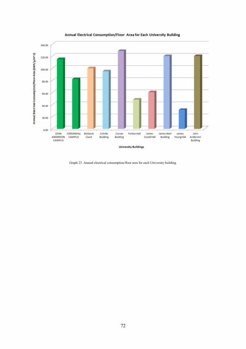
72

Graph 23. Annual electrical consumption/floor area for each University building.

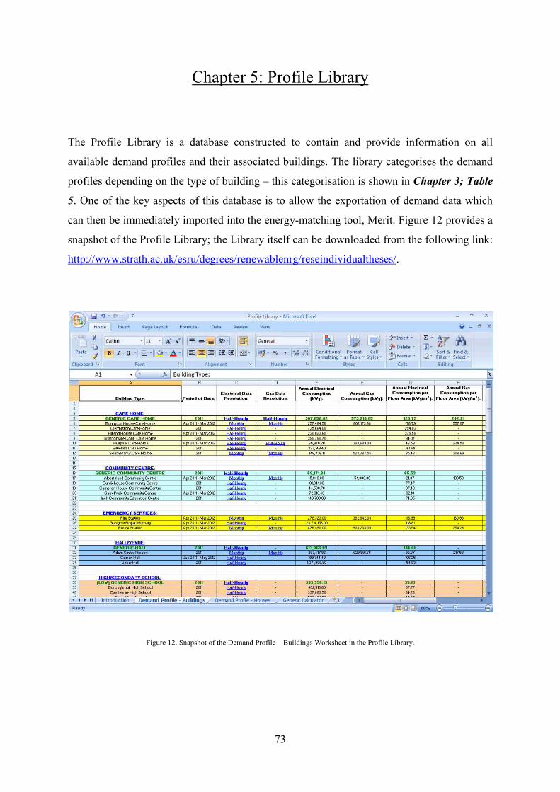
73

Chapter 5: Profile Library

The Profile Library is a database constructed to contain and provide information on all

available demand profiles and their associated buildings. The library categorises the demand

profiles depending on the type of building – this categorisation is shown in Chapter 3; Table

5. One of the key aspects of this database is to allow the exportation of demand data which

can then be immediately imported into the energy-matching tool, Merit. Figure 12 provides a

snapshot of the Profile Library; the Library itself can be downloaded from the following link:

http://www.strath.ac.uk/esru/degrees/renewablenrg/reseindividualtheses/.

Figure 12. Snapshot of the Demand Profile – Buildings Worksheet in the Profile Library.

http://www.strath.ac.uk/esru/degrees/renewablenrg/reseindividualtheses/

74

5.1 Introduction Worksheet

The Profile Library contains an Introduction Worksheet which briefly explains what the

Profile Library is, what it contains and instructions on how to navigate and export the

Demand Profiles in order for them to be imported into Merit. A list of acknowledgments is

also included.

5.2 Demand Profile Worksheets

There are two Worksheets in the Profile Library; one contains information on general

buildings, the other on a number of houses. For each Demand Profile Worksheet, various

pieces of information are shown in a table. Clicking on each building type link (such as Care

Home, Community Centre etc) will take you to the corresponding Excel file within the

database where the user can view a chart depicting the daily average energy consumption

over an annual period for each building type. Each building type Excel file contains charts

and the demand profiles for their associated buildings. These demand profiles are easier to

access through the Demand Profile Worksheets by clicking on the various Data Resolution

links. Please note that all links are highlighted in blue.

5.3 Supply Profile Worksheet

These supply profiles were generated for the demonstration of Merit (which is discussed in

Chapter 7). Similarly to the Demand Profiles, a small database contains relevant information

regarding the renewable technologies such as annual supply generation, wind turbine nominal

power, solar cell voltage at maximum power point etc. These profiles can also be viewed by

clicking on their corresponding Supply Data Resolution.

5.4 Taxonomy

A Generic Profile Taxonomy was created via the website - https://bubbl.us/. This taxonomy

illustrates the Demand Profiles contained within the Profile Library. Due to its size as shown

in Figure 13, it was not possible to fit the entire contents of the taxonomy into this

dissertation without compromising clarity. However, the following read-only link has been

https://bubbl.us/

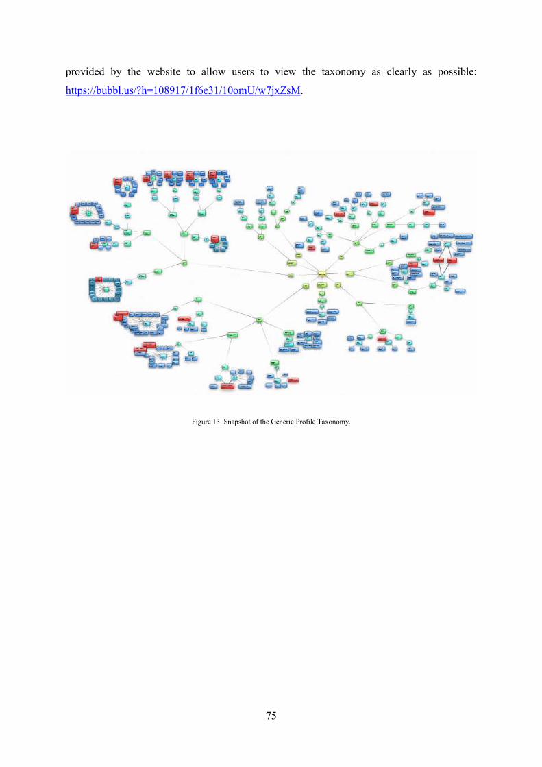
75

provided by the website to allow users to view the taxonomy as clearly as possible:

https://bubbl.us/?h=108917/1f6e31/10omU/w7jxZsM.

Figure 13. Snapshot of the Generic Profile Taxonomy.

https://bubbl.us/?h=108917/1f6e31/10omU/w7jxZsM

76

Chapter 6: Generic Electricity Consumption Calculator

A Generic Electricity Consumption Calculator was developed once all the Generic Demand

Profiles were created and analysed. The calculator, as shown in Figure 14 below, allows the

user to calculate the overall annual electrical consumption for a specific Generic-type of

building (Hall/Venue, Office etc).

Firstly, the user selects the type of building they wish to utilise from a list. Once a building

type is selected, the Generic AECFA and Generic daily occupancy for that building type are

shown in the next two cells, replacing the hyphen. The user can then enter the floor area and

average daily occupancy in the following two cells which would allow an estimated annual

electrical consumption to be calculated.

IMPORTANT: This calculator is based ONLY on the data for the Generic Demand Profiles

and as such, may not accurately match specific buildings (i.e. entering details for Bonnyton

House Care Home from the Profile Library can result in the calculator estimating a dissimilar

value).

77

Figure 14. Snapshot of the Generic Electricity Consumption Calculator in the Profile Library.

Although the Generic Electricity Consumption Calculator is in a very early development

stage, the process in which it operates is still valid and more refinement and demand data are

required in order to expand and improve the accuracy of the calculator.

78

Chapter 7: Analysing the University of Strathclyde with Merit

To better show how the latest version of Merit can be exploited and the effectiveness of such

a DCMT, an example will be used – in this case, the University of Strathclyde.

Please note that the version of Merit used during this dissertation is NOT the final

product and the images of the interface shown below may differ to the latest version.

Two buildings with an electric-demand profile will be used to showcase the supply/demand

matching tool of Merit: James Young, a student accommodation building; and John

Anderson, a teaching and research building. Both buildings consumed contrasting overall

amounts of electricity in 2011 – James Young (56,101 kWh/y) and John Anderson (1,266,497

kWh/y).

A number of supply profiles were generated using renewable technologies such as Proven

Wind Turbines and Sharp Poly Solar PV Panels. Only 3 profiles for each technology were

utilised in Merit, although there were 30 supply profiles created in total. The reason for only

6 profiles used is mainly to demonstrate the execution of Merit. The 6 profiles included

supply data for 1, 5 and 10 Proven WT600 Wind Turbines; 1, 5 and 10 Sharp Poly Solar

Panels.

These profiles were created using weather data from Glasgow in 1972. It is assumed that the

weather for Glasgow from 1972 to 2012 has not changed drastically to affect the results of

Merit.

Once the profiles were imported into Merit, the James Young and John Anderson Demand

Profiles were selected for the Demand Scenario; equally, the same was applied to the supply

profiles for the Supply Scenario. The Matching analysis could now be conducted and is

shown in Figure 15. When this is completed, a list of matches is shown and the optimal

matches for the two Demand Profiles are shown in both Figure 16 and 17.

79

Figure 15. Annotated snapshot of matching interface in Merit.

Graphical

Display

Progress Bar

Matching Analysis

Results

Supply

Profiles

Demand

Profiles

Supply

Scenarios

Demand

Scenarios

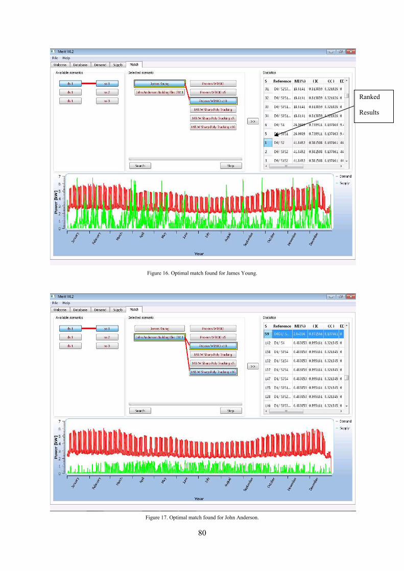
80

Figure 16. Optimal match found for James Young.

Figure 17. Optimal match found for John Anderson.

Ranked

Results

81

The results of Merit have shown that the optimal match for the James Young building with

the renewable technologies corresponded to 10 Proven WT600 wind turbines. The Match

Rate was calculated to be 41.85 %.

In terms of the John Anderson building, the optimal match corresponded to 10 Proven

WT600 wind turbines and 10 165 W Sharp Poly Solar Panels. However, the Match Rate for

this was computed to be only 2.84 %.

This demonstration has shown how Merit can be used to conduct a supply/demand matching

analysis. Those combinations with a significantly high Match Rate could benefit from the

proposed renewable technology.

82

Chapter 8: Conclusions and Future Work

8.1 Conclusion

Over 300 electrical/thermal demand profiles were obtained for various buildings from a range

of sources. These profiles were categorised, refined and analysed with their AECFA, and

AGCFA if applicable, calculated. This allowed Generic Profiles to be developed for a

number of building types such as Schools, Offices, and Houses etc. A Profile Library was

developed which contained relevant information and demand profiles regarding all buildings

used in this project. This database also allows the immediate exportation of demand data for

each individual building which can then be readily imported into a DCMT such as Merit.

Once the Generic Profiles were acquired, a Generic Electricity Consumption Calculator was

developed. This calculator, which is purely based on the data from the Generic Profiles, can

be used to estimate the annual electrical consumption of a specific type of building by scaling

the floor area and average daily occupancy.

A taxonomy was designed to illustrate the demand profiles contained within the Profile

Library and has been categorised to allow clear understanding.

Finally, demand profiles from buildings James Young and John Anderson, part of the

University of Strathclyde, were used with the supply/demand energy matching tool – Merit.

The supply profiles used in collaboration with these demand profiles comprised of data

generation from Wind Turbines and Solar PV Cells. It was found that, with the generated

supply profiles, James Young received an optimal Match Rate of 44.11 % when combined

with 10 Proven WT600 Wind Turbines. John Anderson received an optimal Match Rate of

2.83 % with 10 Proven WT600 Wind Turbines and 10 165 W Sharp Poly Solar Panels.

83

8.2 Future Work

To increase accuracy and effectiveness of the Generic Profiles, more demand profiles could

be collected and analysed. Therefore, those buildings with similar AECFA or AGCFA could

be grouped together just as those done for Offices and Schools.

A more in-depth study could be conducted to not only collect demand profiles for

electrical/thermal consumption but also take into account the electrical appliances in

buildings and how much energy each of those actually consumes, such as lighting,

computers, air-conditioning systems etc. These added factors can then be used to determine a

more accurate Generic Profile which could then be added and exploited in the Generic

Electricity Consumption Calculator where the user can define what type and how many

electrical appliances there are in a specific type of building.

By doing so, it could potentially diminish the need of creating and simulating virtual models

in order to see how much energy a building consumes – thus saving time, money and

resources.

84

References

2020 Route map for Renewable Energy in Scotland (2011). Scottish Government Publication.

Available from: http://www.scotland.gov.uk/Publications/2011/08/04110353/3.

2050 Commercial Lighting and Appliances (2008). Department of Energy & Climate

Change. Available from: 2050-calculator-tool.decc.gov.uk/assets/onepage/44.pdf.

Abulfotuh, F. (2007). 'Energy efficiency and renewable technologies: the way to sustainable

energy future.' Desalination, 209 (1-3), p275-282.

Ackermann, T., Andersson, G. & Söder, L. (2001). 'Overview of Government and market

driven programs for the promotion of renewable power generation.' Renewable Energy, 22

(1-3), p197-204.

Agarwal, Y., Balaji, B., Gupta, R., Lyles, J., Wei, M. & Wng, T. (2010). ‘Occupancy-driven

energy management for smart building automation.’ BuildSys '10 Proceedings of the 2nd

ACM Workshop on Embedded Sensing Systems for Energy-Efficiency in Building, New

York, NY, USA, p1-6.

Almeida, A. D. et al. (2008). 'Final Report REMODECE—Residential Monitoring to

Decrease Energy use and Carbon Emissions in Europe.' IEEA Program Funded Project,

University of Coimbra, Dep. of Electrical Engineering, Pólo II, 3030 290 Coimbra,

Portugal. Available from: http://www.isr.uc.pt/∼remodece/downloads/REMODECE D9

Nov2008 Final.pdf.

Arora, A., Jagannathan, R. & Yi-Min, W. (2002). ‘Model-based fault detection in powerline

networking.’ Parallel and Distributed Processing Symposium., Proceedings International,

IPDPS 2002, Abstracts and CD-ROM , p8-15.

Ashok, S. (2007). ‘Optimised model for community-based hybrid energy system.’ Renewable

Energy, 32, 1155–1164.

85

Atanasiu, B. & Bertoldi, P. (2008). 'Residential electricity consumption in new member states

and candidate countries.' Energy and Buildings, 40 (2) p112–125.

Bang, H. K., Ellinger, A. E., Hadjimarcou, J. & Traichal, P. A. (2000). ‘Consumer concern,

knowledge, belief, and attitude toward renewable energy: An application of the reasoned

action theory.’ Psychology and Marketing, 17, p449–468.

Bertoldi, P. & Atanasiu, B. (2007). 'Electricity Consumption and Efficiency Trends in the

Enlarged European Union.' Status Report 2006 – EUR 22753EN. Institute for Environment

and Sustainability, JRC European Commission.

Borg, S. P. & Kelly, N. J. (2011). 'The effect of appliance energy efficiency improvements on

domestic electric loads in European households.' Energy and Buildings, 43, p2240-2250.

Born, F. J. (2001). ‘Aiding Renewable Energy Integration through Complimentary Demand-

Supply Matching.’ PhD Thesis, University of Strathclyde.

Burch, G, D. (2001). ‘Hybrid Renewable Energy Systems.’ U.S. DOE Natural Gas /

Renewable Energy Workshops, Golden, Colorado.

Chwieduk, D. (2003). ‘Towards sustainable-energy buildings.’ Applied Energy, 76, p211-

217.

Curran, J., Fenton, N. & Freedman, D. E. S. (2012). ‘Misunderstanding the internet.’

Communication and society, Routledge.

Deshmukh, M. K. & Deshmukh, S.S. (2008). ‘Modeling of hybrid renewable energy

systems.’ Renewable and Sustainable Energy Reviews, 12 (1), p235-249.

DG for Energy and Transport, EU Energy and Transport in Figures European Commission,

DG for Energy and Transport, Brussels. (2009). Available from:

http://ec.europa.eu/energy/publications/statistics/doc/2009 energy transport figures.pdf.

86

Doherty, P. S., Al-Huthaili, S., Riffat, S. B. & Abodahab, N. (2004). 'Ground source heat

pump––description and preliminary results of the Eco House system.' Applied Thermal

Engineering, 24 (17-18), p2627-2641.

DUKES - Digest of United Kingdom Energy Statistics. (2011). Available from:

http://www.decc.gov.uk/en/content/cms/statistics/publications/dukes/dukes.aspx.

Ekren, O. & Ekren, B. Y. (2008). ‘Size optimization of a PV/wind hybrid energy conversion

system with battery storage using response surface methodology.’ Applied Energy, 85,

p1086–1101.

Eldridge, M. et al. (2008). 'Energy Efficiency: The first fuel for a clean energy future.'

Maryland Efficiency Potential, ACEEE, Report Number E082, p1-119.

Energy in Sweden facts and figures 2010. (2010). Swedish Energy Agency. Available from:

http://webbshop.cm.se/System/TemplateView.aspx?p=Energimyndigheten&view=default&

cat=/Broschyrer&id=e0a2619a83294099a16519a0b5edd26f.

Fischer, C. (2008). 'Feedback on household electricity consumption: a tool for saving

energy?' Energy Efficiency, 1 (1), p79-104.

Guo, X. L., Ni, M. F., Lin, W. P. & Wu, X. P. (2011). ‘The review and summary of the

research on Life Cycle Assessment.’ Advanced Materials Research, 347-353, p2768-2772.

HM Government (2008). ‘Improving the energy efficiency of our homes and buildings.

Energy Certificates and air-conditioning inspections for buildings.’ Department for

Communities and Local Government. Available from:

http://www.communities.gov.uk/documents/planningandbuilding/pdf/714826.pdf.

Hseih, T. T., Chiang, C. M., Ho, M., C. & Lai, K., P. (2011). ‘The Application of Green

Building Materials to Sustainable Building for Environmental Protection in Taiwan.’

Advanced Materials Research, 343-344, p267-272.

87

Hvelplund, F. (2006). 'Renewable energy and the need for local energy markets.' Energy, 31

(13), p2293-2302.

Kelly, N. J. & Cockroft, J. (2011). 'Analysis of retrofit air source heat pump performance:

Results from detailed simulations and comparison to field trial data.' Energy and Buildings,

43 (1), p239-245.

Langhammer, N. & Kays, R. (2011). ‘Evaluation of wireless smart metering technologies in

realistic indoor channels.’ Wireless Communication Systems (ISWCS), 2011 8th

International Symposium on , p387-391.

Lee, R. G. M., Coleman, P., Jones, J. L., Jones, K. C. & Lohmann, R. (2005). 'Emission

Factors and Importance of PCDD/Fs, PCBs, PCNs, PAHs and PM10 from the Domestic

Burning of Coal and Wood in the U.K.' Environmental Science & Technology, 39 (6),

p1436-1447.

Legislation: Freedom of Information Act, 2000. Available from:

http://www.legislation.gov.uk/ukpga/2000/36/contents.

Legislation: Freedom of Information (Scotland) Act, 2002. Available from:

http://www.legislation.gov.uk/asp/2002/13/contents.

Mitchell, C. & Connor, P. (2004). 'Renewable energy policy in the UK 1990–2003.' Energy

Policy, 32 (17), p1935-1947.

M’Sirdi, N., Namaane, A.,Howlett, R. J. & Lakhmi, C. J. (2012). ‘Sustainability in Energy

and Buildings: Proceedings of the 3rd International Conference in Sustainability in Energy

and Buildings.’ Smart Innovation, Systems and Technologies, 12, p1-560.

Nast, M., Langniß, O. & Leprich, U. (2007). 'Instruments to promote renewable energy in the

German heat market—Renewable Heat Sources Act.' Renewable Energy, 32 (7), p1127-

1135.

88

Omer, A. M. (2008). 'Ground-source heat pumps systems and applications.' Renewable and

Sustainable Energy Reviews, 12 (2), p344-371.

Pidgeon, N. F., Lorenzoni, I. & Poortinga, W. (2008). 'Climate change or nuclear power—No

thanks! A quantitative study of public perceptions and risk framing in Britain.' Global

Environmental Change, 18 (1) p69-85.

Quantitative Research into Public Awareness, Attitudes, and Experience of Smart Meters.

(2012). Department of Energy & Climate Change. Available from:

http://www.decc.gov.uk/assets/decc/11/tackling-climate-change/smart-meters/6194-

quantitative-research-into-public-awareness-attit.pdf.

Ramakumar, R. & Chiradeja, P. (2002). 'Distributed generation and renewable energy

systems.' Energy Conversion Engineering Conference, 2002. IECEC '02. 2002 37th

Intersociety, p716-724.

Rodolfo, D. L., José, L., Bernal A. ‘Multi-objective design of PV-wind-diesel-hydrogen

battery systems.’ Renewable Energy, 33, p2559-2572.

Ruta, M., Scioscia, F., Di Sciascio, E. & Loseto, G. (2011). ‘A semantic-based evolution of

EIB Konnex protocol standard.’ Mechatronics (ICM), 2011 IEEE International Conference

on , p773-778.

Scheaffer, R. L. & McClave, J. T. (1982). ‘Statistics for Engineers.’ PWS Publishers.

Smart Meter Testing & Trialling Discussion Paper, ERA – SRSM Group. (2011). ENERGY

RETAIL Association. Available from: http://www.energy-uk.org.uk/publication/finish/37-

smart-meter-policies/525-smart-meter-testing-and-trialling-paper.html.

Smith, L. (2011). The Green Deal. House of Commons Library. London, House of

Commons.

89

Upreti, B. R. & van der Horst, D. (2004). 'National renewable energy policy and local

opposition in the UK: the failed development of a biomass electricity plant.' Biomass and

Bioenergy, 26 (1), p61-69.

Weiss, W. W. (2003). 'Solar Heating Systems for Houses: A Design Handbook for Solar

Combisystems.' International Energy Agency. Solar Heating and Cooling Programme, p1-

313.

Williamson, T. J. (1994). ‘A confirmation technique for thermal performance simulation

models.’ University of Adelaide, Australia.

Xue, J. H. & Li, H., M. (2011). ‘Firms and Governments behaviours for sustainable-buildings

energy saving.’ Advanced Materials Research, 374-377, p14-17.

Yang, G. F., Guo, Y. & Wang, L. (2012). ‘Application of the Direct-Gain Passive Solar

House on Middle and Small-Sized Public Building.’ Advanced Materials Research, 450-

451, p1429-1434.

Yu, J. Q., Dang, B., Clements-Croome, D. & Xu, S. (2011). ‘Sustainability assessment

indicators and methodology for intelligent buildings.’ Advanced Materials Research, 368-

373, p3829-3832.

Yu-Ju, L., Latchman, H.A., Minkyu, L. & Katar, S. (2002). ‘A power line communication

network infrastructure for the smart home.’ Wireless Communications, IEEE , 9 (6), p104-

111.

90

Appendices

Appendix 1: Map of Scottish Regions

Source: http://www.scotland.gov.uk/Publications/2004/06/19506/38901.

http://www.scotland.gov.uk/Publications/2004/06/19506/38901

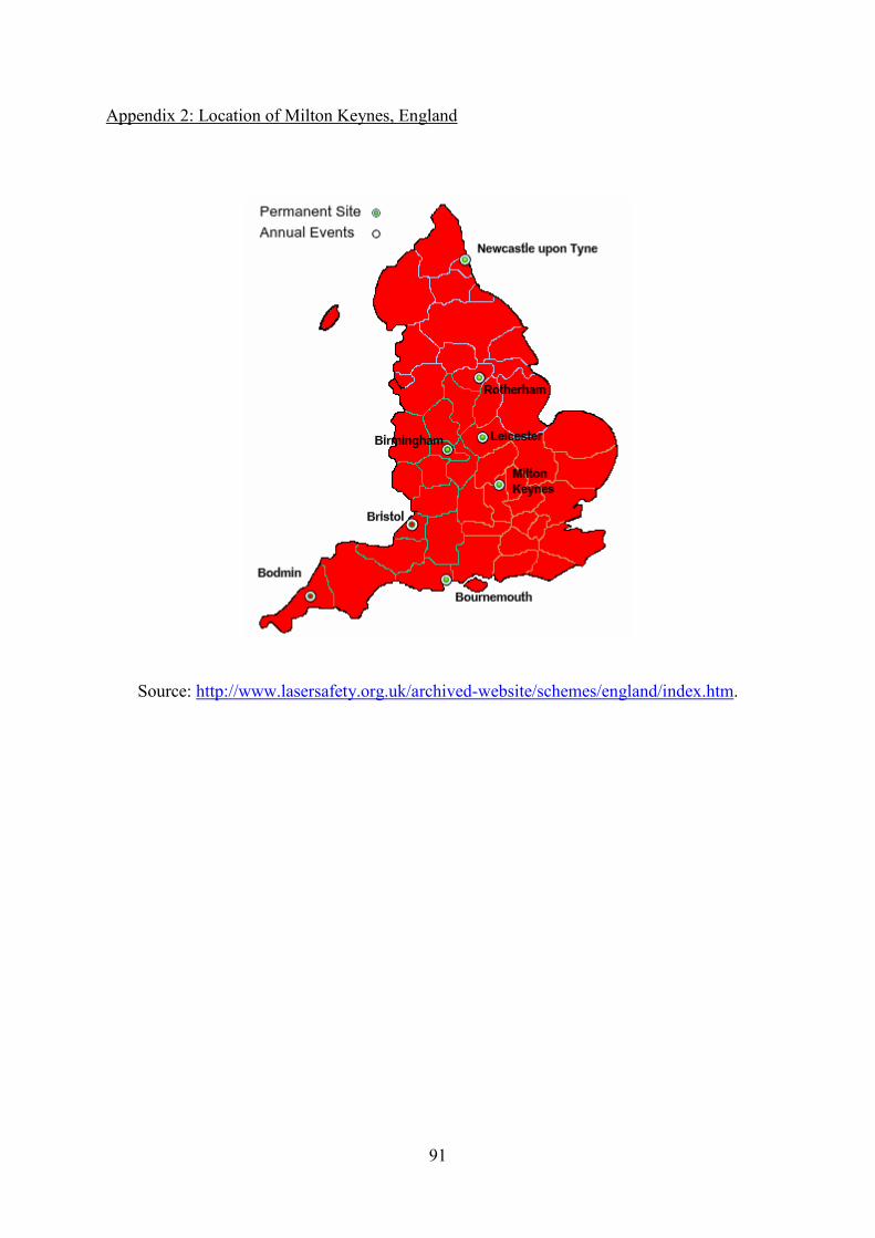
91

Appendix 2: Location of Milton Keynes, England

Source: http://www.lasersafety.org.uk/archived-website/schemes/england/index.htm.

http://www.lasersafety.org.uk/archived-website/schemes/england/index.htm

Generic Energy Demand Profile Generation - Strath Energy Demand Profile Generation ... supply/demand...

Documents

Transcript of Generic Energy Demand Profile Generation - Strath Energy Demand Profile Generation ... supply/demand...