Generalized Functions for the Fractional Calculus€¦ · Generalized Functions for the Fractional...
24
NASA/TP—1999-209424/REV1 October 1999 Carl F. Lorenzo Glenn Research Center, Cleveland, Ohio Tom T. Hartley The University of Akron, Akron, Ohio Generalized Functions for the Fractional Calculus
Transcript of Generalized Functions for the Fractional Calculus€¦ · Generalized Functions for the Fractional...

NASA/TP—1999-209424/REV1
October 1999
Carl F. LorenzoGlenn Research Center, Cleveland, Ohio
Tom T. HartleyThe University of Akron, Akron, Ohio
Generalized Functions for theFractional Calculus

The NASA STI Program Office . . . in Profile
Since its founding, NASA has been dedicated tothe advancement of aeronautics and spacescience. The NASA Scientific and TechnicalInformation (STI) Program Office plays a key partin helping NASA maintain this important role.
The NASA STI Program Office is operated byLangley Research Center, the Lead Center forNASA’s scientific and technical information. TheNASA STI Program Office provides access to theNASA STI Database, the largest collection ofaeronautical and space science STI in the world.The Program Office is also NASA’s institutionalmechanism for disseminating the results of itsresearch and development activities. These resultsare published by NASA in the NASA STI ReportSeries, which includes the following report types:
• TECHNICAL PUBLICATION. Reports ofcompleted research or a major significantphase of research that present the results ofNASA programs and include extensive dataor theoretical analysis. Includes compilationsof significant scientific and technical data andinformation deemed to be of continuingreference value. NASA’s counterpart of peer-reviewed formal professional papers buthas less stringent limitations on manuscriptlength and extent of graphic presentations.
• TECHNICAL MEMORANDUM. Scientificand technical findings that are preliminary orof specialized interest, e.g., quick releasereports, working papers, and bibliographiesthat contain minimal annotation. Does notcontain extensive analysis.
• CONTRACTOR REPORT. Scientific andtechnical findings by NASA-sponsoredcontractors and grantees.
• CONFERENCE PUBLICATION. Collectedpapers from scientific and technicalconferences, symposia, seminars, or othermeetings sponsored or cosponsored byNASA.
• SPECIAL PUBLICATION. Scientific,technical, or historical information fromNASA programs, projects, and missions,often concerned with subjects havingsubstantial public interest.
• TECHNICAL TRANSLATION. English-language translations of foreign scientificand technical material pertinent to NASA’smission.
Specialized services that complement the STIProgram Office’s diverse offerings includecreating custom thesauri, building customizeddata bases, organizing and publishing researchresults . . . even providing videos.
For more information about the NASA STIProgram Office, see the following:
• Access the NASA STI Program Home Pageat http://www.sti.nasa.gov
• E-mail your question via the Internet [email protected]
• Fax your question to the NASA AccessHelp Desk at (301) 621-0134
• Telephone the NASA Access Help Desk at(301) 621-0390
• Write to: NASA Access Help Desk NASA Center for AeroSpace Information 7121 Standard Drive Hanover, MD 21076

Carl F. LorenzoGlenn Research Center, Cleveland, Ohio
Tom T. HartleyThe University of Akron, Akron, Ohio
Generalized Functions for theFractional Calculus
NASA/TP—1999-209424/REV1
October 1999
National Aeronautics andSpace Administration
Glenn Research Center

Available from
NASA Center for Aerospace Information7121 Standard DriveHanover, MD 21076Price Code: A03
National Technical Information Service5285 Port Royal RoadSpringfield, VA 22100
Price Code: A03

NASA/TP—1999-209424 1
Generalized Functions for the Fractional Calculus
Carl F. LorenzoNational Aeronautics and Space Administration
Glenn Research CenterCleveland, Ohio 44135
Tom T. HartleyThe University of Akron
Department of Electrical EngineeringAkron, Ohio 44325–3904
Introduction Previous papers have used two important functions for the solution of fractional order
differential equations, the Mittag-Leffler function [ ]qq atE (1903a, 1903b, 1905), and the
F-function [ ]F a tq , of Hartley & Lorenzo (1998). These functions provided direct solution and
important understanding for the fundamental linear fractional order differential equation and forthe related initial value problem (Hartley and Lorenzo, 1999). This paper examines related functions and their Laplace transforms. Presented forconsideration are two generalized functions, the R -function and the G -function, useful inanalysis and as a basis for computation in the fractional calculus. The R -function is unique inthat it contains all of the derivatives and integrals of the F-function. The R -function also returnsitself on qth order differ-integration. An example application of the R -function is provided. Afurther generalization of the R -function, called the G -function brings in the effects of repeatedand partially repeated fractional poles.
Functions for the Fractional Calculus This section summarizes a number of functions that have been found useful in the solutionof problems of the fractional calculus and more particularly in the solution of fractionaldifferential equations.
Mittag-Leffler FunctionThe Mittag-Leffler (1903, 1903, 1905) function is given by the following equation
[ ] ( ) ( )1.0,10
>+Γ
=∑∞
=
qnq
ttE
n
n
q
This function will often appear with the argument −at q , its Laplace transform then, is given as
[ ]{ } ( )( ) ( ) ( )2.0
10
>+
=
+Γ−=− ∑
∞
=
qass
s
nq
taLatEL
q
q
n
nqnq
q

2
Agarwal’s FunctionThe Mittag-Leffler function is generalized by Agarwal (1953) as follows
( ) ( ) ( )∑∞
=
−
+
+Γ=
0
1
, 3.m
m
m
ttE
βα
αβ
βα
This function is particularly interesting to the fractional order system theory due to its Laplacetransform, given by Agarwal as
[ ]{ } ( )4.1, −
=−
α
βαα
βα s
stEL
This function is the ( )α β− order fractional derivative of the F-function, (of Robotnov (1969)
and Hartley (1998)), with argument a =1, to be presented later.
Erdelyi’s FunctionErdelyi (1954) has studied the following related generalization of the Mittag-Leffler function
( ) ( ) ( )5,0,,0
, >+Γ
=∑∞
=
βαβαβα
m
m
m
ttE
where the powers of t are integer. The Laplace transform of this function is given by
( ){ } ( )( ) ( )6.0,
1
01, >
+Γ+Γ=∑
∞
=+ βα
βαβαm
msm
mtEL
As this function cannot be easily generalized it will not be considered further.
Robotnov and Hartley’s FunctionTo effect the direct solution of the fundamental linear fractional order differential equation
the following function was introduced (Hartley and Lorenzo, 1998)
[ ] ( )( ) ( )7.0,
0
1 >+Γ
−=− ∑∞
=
− qqnq
tattaF
n
nqnq
q
This function had been studied earlier by Robotnov (1969, 1980) with respect to hereditaryintegrals for application to solid mechanics. The important feature of this function is the powerand simplicity of its Laplace transform, namely
[ ]{ } ( )8.0,1
, >−
= qas
taFLqq
Miller and Ross’ FunctionMiller and Ross (1993, pp.80 and 309-351) introduce another function as the basis of the
solution of the fractional order initial value problem. It is defined as the v th integral of theexponential function, that is
( ) ( ) ( )( ) ( )9,
1,,
0∑∞
=
∗−
−
++Γ===
k
kvatvat
v
v
t kv
attatvete
dt
davE γ
NASA/TP—1999-209424

3
where ( )γ ∗ v at, is the incomplete gamma function. The Laplace transform of equation (9)follows directly as
( ){ } ( ) ( )10.1Re, >−
=−
vas
savEL
v
t
Miller and Ross then show that
( ) ( )11,...,3
1,
2
1,1
1,...3,2,1,
1,1
1
1 ===−
=
−∑=
−
qvq
asajvEaL
v
jt
j
which is a special case of the F-function of Robotnov and Hartley.
The above functions are studied in considerable detail by their originators and others. Theinterested reader is directed to the supplied references.
A Generalized Function It is of significant usefulness to develop a generalized function which when fractionallydifferintegrated (by any order) returns itself. Such a function would greatly ease the analysisof fractional order differential equations. To this end the following is proposed, considerthe function
[ ] ( ) ( )( )
( )( ) ( )12.1
,,0
11
, ∑∞
=
−−+
−+Γ−≡
n
vqnn
vq vqn
ctatcaR
Our interest in this function will normally be for the solution of fractional differential equationsfor the range of .0=> ct For Rct ,< will be complex except for the cases when the exponent
( )( )vqn −−+ 11 is integer. The more compact notation
[ ] ( ) ( )( )
( )( ) ( )13,1
,0
11
, ∑∞
=
−−+
−+Γ−=−
n
vqnn
vq vqn
ctactaR
is also useful, particularly when c = 0.The Laplace transform of the R -function is
[ ]{ } ( ) ( )( )
( )( ) ( ) ( )( )
( )( ) ( )14.11
,,0
11
0
11
, ∑∑∞
=
−−+∞
=
−−+
−+Γ−=
−+Γ−=
n
vqnn
n
vqnn
vq vqn
ctLa
vqn
ctaLtcaRL
Consider first the case for c = 0, then we have
[ ]{ } ( ) ( )( )
( )( ) ( )15.1
,0,0
11
, ∑∞
=
−−+
−+Γ=
n
vqnn
vq vqn
tLataRL
Now from (Erdelyi et al, 1954)
{ } ( ) ( ) ( ) ( )16.0Re,1Re1 1 >−>+Γ= −− svsvtL vv
Then equation 15 becomes
[ ]{ } ( ) ( ) ( )( ) ( ) ( )17.0Re,01Re1
,0,0
1, ∑∞
=−+ >>−+=
nvqn
nvq svqn
sataRL
NASA/TP—1999-209424

NASA/TP—1999-209424 4
[ ]{ } ( )( ) ( )( ) ( ) ( )18.0Re,01Re
1,0,
01, ∑
∞
=+− >>−+=
nqn
n
vvq svqns
a
staRL
This can be written as a geometric series that converges when .1<qsa It can be shown, by
long division, that
( ){ } ( ) ( ) ( )19.0sRe,0Re,,0,, >>−−
= vqas
staRL
q
v
vq
Now for c ≠ 0the shifting theorem for the Laplace transform (Wylie p. 281) is
( ) ( ){ } ( ){ } ( )20,0≥=−− − btfLebtubtfL bs
where the unit step function ( )u t b− effectively causes ( )f t b− = 0for t b< . Under the
assumption that [ ] 0,,, =tcaR vq for t c< , this theorem and the result (equation 19) are applied
to yield
( ){ } ( )( ) ( )21.0Re,01Re,0,,, >>−+≥−
=−
svqncas
setcaRL
q
vcs
vq
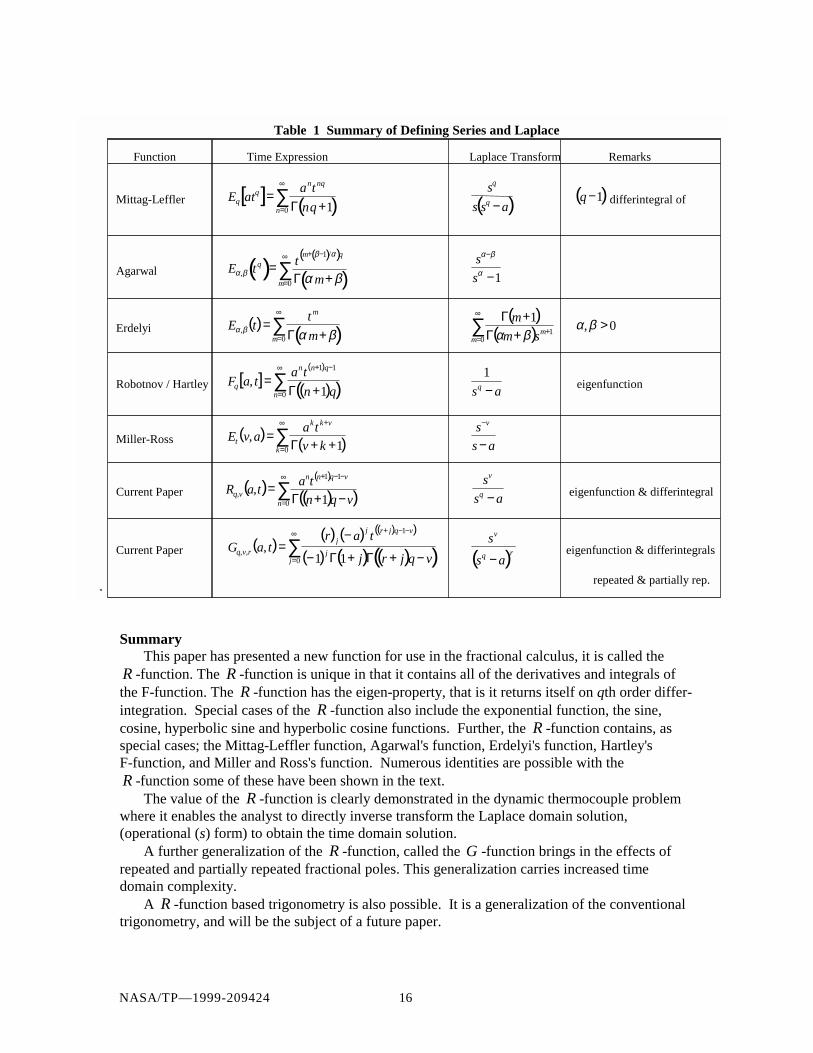
Table 1, in a later section, presents a summary of the defining series and respective Laplacetransforms for the functions discussed in this paper.
Properties of the Rq,v(a,c,t)FunctionThe general time domain character of the R -function is shown in figures 1, 2, and 3. Figure 1shows the effect of variations in q with 0=v and .1±=a The exponential character of the
function is readily observed (see, q =1). Figure 2 shows the effect of v on the behavior of the
R -function. The effect of the characteristic time a is shown in figure 3. The characteristic time is
1/ aq . For q a=1 1, / is the time constant, when q = 2 we have the natural frequency, when qtakes on other values we have the generalized characteristic time (or generalized time constant).
Figure 1b. Effect of q on ( ),,0,10, tRq −0.1,0.0 −== av
Figure 1a. Effect of q on ( ),,0,10, tRq0.1,0.0 == av

5
( )tRv v ,0,1on ,25.0 −0.1,25.0 −== aq
Figure 2b. Effect of ( )tRv v ,0,1on ,50.0 −0.1,50.0 −== aq
Figure 2c. Effect of ( )tRv v ,0,1on ,75.0 −0.1,75.0 −== aq
Figure 2a. Effect of
Figure 2d. Effect of ( )tRv v ,0,1on ,00.1 −0.1,00.1 −== aq
0 0.1 0.2 0.3 0.4 0.5 0.6 0.7 0.8 0.9 1-1
-0.5
0
0.5
1
1.5
2
t
R-F
unctionR(0.25,v,-1,0,t)
v= -0.45
v= 0.15
v= -0.45 to v= 0.15 in steps of 0.15
a= -1.0, q=0.25
v=0.00
0 0.1 0.2 0.3 0.4 0.5 0.6 0.7 0.8 0.9 1-1
-0.5
0
0.5
1
1.5
2
t
R-F
unctionR(0.50,v,-1,0,t)
v= -0.45
v= 0.45
v= -0.45 to v= 0.45 in steps of 0.15
a= -1.0, q=0.50
v=0.00
v=0.15v=0.30
0 0.1 0.2 0.3 0.4 0.5 0.6 0.7 0.8 0.9 1-1
-0.5
0
0.5
1
1.5
2
t
R-F
unctionR(0.75,v,-1,0,t)
v= -0.45
v= 0.60
v= -0.45 to v= 0.60 in steps of 0.15
a= -1.0, q=0.75
v=0.00v=0.15v=0.30
0 0.1 0.2 0.3 0.4 0.5 0.6 0.7 0.8 0.9 1-1
-0.5
0
0.5
1
1.5
2
t
R-F
unctionR(1.00,v,-1,0,t)
v= -0.45
v= 0.60
v= -0.45 to v= 0.90 in steps of 0.15
a= -1.0, q=1.00
v=0.00v=0.15v=0.30
v=0.75
v=0.90
NASA/TP—1999-209424

6
0 0.5 1 1.5 2 2.5 3-0.5
0
0.5
1
1.5
2
t
R-FunctionR(1.0,0,a,0,t)
a= 0.00
a= 0.50
a= -2.0 to 0.5 in steps of 0.5
a= -2.00
q=1.0, v= 0.0
a= -0.50
0 0.5 1 1.5 2 2.5 3
-0.5
0
0.5
1
1.5
2
t
R-FunctionR(0.50,0,a,0,t)
a= 0.00
a= 0.50a= -2.0 to 0.5 in steps of 0.5
a= -2.00
q=0.50, v= 0.0
a= -0.50
Figure 3d. Effect of a ( )taR ,0,on 0,00.1
0.0,00.1 == vq
Figure 3a. Effect of a ( )taR ,0,on 0,25.0
0.0,00.1 == vqFigure 3b. Effect of a ( )taR ,0,on 0,50.0
0.0,50.0 == vq
Figure 3c. Effect of a ( )taR ,0,on 0,75.0
0.0,75.0 == vq
0 0.5 1 1.5 2 2.5 3-0.5
0
0.5
1
1.5
2
t
R-F
unctionR(0.75,0,a,0,t)
a= 0.00
a= 0.50
a= -2.0 to 0.5 in steps of 0.5
a= -2.00
q=0.75, v= 0.0
a= -0.50
0 0.5 1 1.5 2 2.5 3-0.5
0
0.5
1
1.5
2
t
R-F
unctionR(0.25,0,a,0,t)
a= 0.00
a= 0.50
a= -2.0 to 0.5 in steps of 0.5
a= -2.00
q=0.25, v= 0.0
a= -0.50
NASA/TP—1999-209424
NASA/TP—1999-209424 7
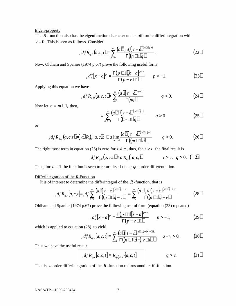
Eigen-propertyThe R -function also has the eigenfunction character under qth order differintegration with
.0=v This is seen as follows. Consider
( ) ( ) ( )( )
( )( ) ( )22.1
,,0
11
0, ∑∞
=
−+
+Γ−
=n
qnqtc
n
qqtc qn
ctdatcaRd
Now, Oldham and Spanier (1974 p.67) prove the following useful form
[ ] ( )[ ]( ) ( )23.1
1
1 −>+−Γ−+Γ=−
−
pvp
axpaxd
vppv
xa
Applying this equation we have
( ) ( ) ( )( ) ( )24.0,,
0
1
0, >Γ
−= ∑∞
=
−
qnq
ctatcaRd
n
nqn
qqtc
Now let n m= +1, then,
( ) ( )( )
( )( ) ( )25011
111
>+Γ
−= ∑∞
−=
−++
qqm
cta
m
qmm
or
( ) ( ) ( ) ( ) ( )( )
( )( ) ( )26.01
lim,,,,11
-1m0,0, >
+Γ−+=
−+
→q
qm
ctaatcaRatcaRd
qmm
qqqtc
The right most term in equation (26) is zero for ct ≠ , thus, for ct > the final result is
( ) ( ) ( )27.0,,,,, 0,0, >>= qcttcaRatcaRd qqqtc
Thus, for 1=a the function is seen to return itself under qth order differentiation.
Differintegration of the R-FunctionIt is of interest to determine the differintegral of the R -function, that is
[ ] ( ) ( )( )
( )( )( ) ( )( )
( )( ) ( )28.11
,,0 0
1111
, ∑ ∑∞
=
∞
=
−−+−−+
−+Γ−=
−+Γ−=
n n
vqnutc
nvqnnutcvq
utc vqn
ctda
vqn
ctadtcaRd
Oldham and Spanier (1974 p.67) prove the following useful form (equation (23) repeated)
[ ] ( )[ ]( ) ( )29,1
1
1 −>+−Γ−+Γ=−
−
pvp
axpaxd
vppv
xa
which is applied to equation (28) to yield
[ ] ( ) ( )( ) ( )
( ) ( )( ) ( )30.01
,,0
11
, >−+−+Γ
−= ∑∞
=
+−−+
vquvqn
ctatcaRd
n
uvqnn
vqutc
Thus we have the useful result
[ ] ( )[ ] ( )31.,,,, ,, vqtcaRtcaRd uvqvqutc >= +
That is, u order differintegration of the R -function returns another R -function.

8
Relationship Between mqq,R and 0,qR
From the definition of R we can write
( ) ( ) ( )( )
( )( ) ( ) ( ) ( )( )
( )( ) ( )32.11
,,0
11
0
11
, ∑∑∞
=
−+−
∞
=
−−+
+−Γ−−=
−+Γ−=
n
qnnmq
n
mqqnn
mqq qmn
ctact
mqqn
ctatcaR
Letting n m r− = , yields
( ) ( ) ( ) ( )( )
( )( ) ( )33,1
,,11
, ∑∞
−=
−+++−
+Γ−−=
mr
qmrmrmq
mqq qr
ctacttcaR
or
( ) ( ) ( ) ( )( )
( )( ) ( ) ( ) ( )( )
( )( ) ( )34.11
,,1 11
0
11
, ∑∑−
−=
−+∞
=
−+
+Γ−+
+Γ−=
mr
qrrm
r
qrrm
mqq qr
ctaa
qr
ctaatcaR
Recognizing the first summation on the right hand side as ( ),,,0, tcaRq gives the final result as;
( ) ( ) ( ) ( ) ( ) ( )( )
( )( ) ( )35.1
,,,,1 11
0,, ∑−
−=
−+
+Γ−+=
mr
qrrm
qm
mqq qr
ctaatcaRatcaR
It is noted, that when ( )r q+ ≤1 0 and integer the elements of the summation term vanish.
Fractional Impulse FunctionConsider the function ( ),,0,00, tRq then we can write,
( ) ( ) ( ) ( )
( )( ) ( )36.1
lim,0,lim,0,00
11
00,
00, ∑
∞
=
−+
→→ +Γ==
n
qnn
aq
aq qn
tataRtR
In the limit the terms n > 0, of the summation vanish, thus
( ) ( )( ) ( ) ( )37.lim,0,
110
00,
q
t
q
tataR
aq Γ
=Γ
=−−
→
From equation (19) the associated Laplace transform pair is given by;
( ){ } ( ) ( ) ( )38.0Re,0Re1
,0,00, >>= sqs
tRLqq
Relationship of the R-function to the Elementary Functions Many of the elementary functions are special cases of the R -function. Some of these areillustrated here.
Exponential Function Consider ( )taR ,0,0,1 , by definition, we have
( ) ( )( )
( ) ( )39,!1
,0,0 0
0,1 ∑ ∑∞
=
∞
=
=+Γ
=n n
nnn
n
at
n
tataR
thus
( ) ( )40.,0,0,1taetaR =
NASA/TP—1999-209424

9
Sine Function
Consider ( )taRa ,0,20,2 − , by definition, we have
( ) ( ) ( )
( ) ( )41,....!5!3!12
,0,5432
0
12122
0,2
−+−=+
−=− ∑∞
=
−+ tatata
n
taataRa
n
nn
thus
( ) ( ) ( )42.sin,0,20,2 attaRa =−
Cosine Function
The cosine function relates to ( ),,0,21,2 taR − again by definition
( ) ( ) ( )
( )( )( )( ) ( )43,....
!4!21
!2121,0,
4422
0
22
0
112122
1,2
−+−=−=−+Γ
−=− ∑∑∞
=
∞
=
−−+ tata
n
ta
n
tataR
n
nn
n
nn
thus
( ) ( ) ( )44.cos,0,21,2 tataR =−
Hyperbolic Sine and Cosine
Consider ( )taRa ,0,20,2 , by definition, we have
( ) ( ) ( )
( )( )( )( ) ( )45,...
!5!3!1221,0,
5533
0
122
0
12122
0,2
+++=+
=+Γ
= ∑∑∞
=
+∞
=
−+ tatata
n
taa
n
taataRa
n
nn
n
nn
thus,
( ) ( ) ( )46.sinh,0,20,2 tataRa =
In similar manner
( ) ( ) ( )47.cosh,0,21,2 tataR =
R-Function Identities
Trigonometric Based IdentitiesA number of identities involving the R -function may be readily shown based on the
elementary functions. The exponential function, equation (40)
( ) ( )48,,0,0,1xaexaR =
may be expressed as
( ) ( )49.,0,0,1 xiRe xi = Then from equation (42)
( ) ( ) ( )50,,0,sin 20,2 xaRaax −=
and expressing the sine function in complex exponential terms gives
( ) ( ) ( )51.2
1sin xixi ee
ix −−=
NASA/TP—1999-209424

10
Combining equations (49) ,(50) and (51) then yields the identity
( ) ( ) ( )( ) ( )52.,0,-02
1,0,1 1,00,10,2 xiR,xi,R
ixR −=−
In similar manner using the cosine function, equation (44)
( ) ( ) ( ) ( )53,2
1,0,1cos 1,2
xixi eexRx −+=−=
from which
( ) ( ) ( )( ) ( )54.,0,+02
1,0,1 1,00,11,2 xiR,xi,RxR −=−
The hyperbolic functions may also be used as a basis, using sinh function, yields
( ) ( ) ( )( ) ( )55.,0,1-012
1,0,1 1,00,10,2 xR,x,RxR −=
The cosh function gives
( ) ( ) ( )( ) ( )56.,0,1+012
1,0,1 1,00,11,2 xR,x,RxR −=
Many other identities may be found based on the known trigonometric identities, a few examplesfollow, from
( ) ( ) ( )57,1cossin 22 =+ xx
we have
( ) ( ) ( )58.1,0,1,0,1 22,1
22,0 =−+− xRxR
From the identity
( ) ( ) ( ) ( )59,cossin22sin xxx =
derives( ) ( ) ( ) ( )60.,0,1,0,122,0,1 1,20,20,2 xRxRxR −−=−
From the trigonometric identity
( ) ( ) ( ) ( )61,sin4sin33sin 3 xxx −=
we determine the identity
( ) ( ) ( ) ( )62.,0,14,0,133,0,1 32,00,20,2 xRxRxR −−−=−
Further IdentitiesOther identities may be derived as follows. Let v q p= − , then the Laplace transform of the
R -function may be written as
( ){ } ( ) ( )63.1s
=,0,, assastaRL
qqpq
pq
pqq +=
+− −
−
−
NASA/TP—1999-209424
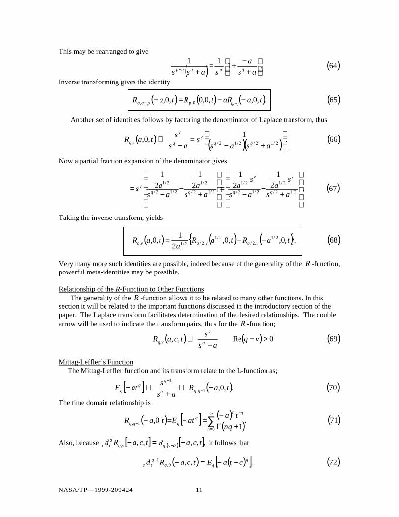
11
This may be rearranged to give
( ) ( )64.111
+−+=
+− as
a
sass qpqqp
Inverse transforming gives the identity
( ) ( ) ( ) ( )65.,0,,0,0=,0, 0,, taaRtRtaR ppqq −−−−
Another set of identities follows by factoring the denominator of Laplace transform, thus
( ) ( )( ) ( )66.1
,0,2/12/2/12/
+−
=−
⇔asas
sas
staR
v
q
v
q,v
Now a partial fraction expansion of the denominator gives
( )67.2
1
2
1
2
1
2
1
2/12/
2/1
2/12/
2/1
2/12/
2/1
2/12/
2/1
+−
−=
+−
−=
as
sa
as
sa
asa
asas
q
v
q
v
qqv
Taking the inverse transform, yields
( ) ( ) ( ){ } ( )68.,0,,0,2
1,0, 2/1
,2/2/1
,2/2/1 taRtaRa
taR vqvqq,v −−=
Very many more such identities are possible, indeed because of the generality of the R -function,powerful meta-identities may be possible.
Relationship of the R-Function to Other FunctionsThe generality of the R -function allows it to be related to many other functions. In this
section it will be related to the important functions discussed in the introductory section of thepaper. The Laplace transform facilitates determination of the desired relationships. The doublearrow will be used to indicate the transform pairs, thus for the R -function;
( ) ( ) ( )690Re,,, >−−
⇔ vqas
stcaR
q
v
vq
Mittag-Leffler’s Function The Mittag-Leffler function and its transform relate to the L-function as;
[ ] ( ) ( )70.,0,1,
1
taRas
satE qqq
q −⇔+
⇔− −
−
The time domain relationship is
( ) [ ] ( )( ) ( )71.
1,0,
01, ∑
∞
=− +Γ
−=−=−n
nqnq
qqq qn
tataEtaR
Also, because [ ] ( )[ ],,,,, ,, tcaRtcaRd vqvqtc −=− +αα it follows that
( ) ( )[ ] ( )72.,,0,1 q
qqqtc ctaEtcaRd −−=−−
NASA/TP—1999-209424
pq −,

12
Argarwal’s FunctionThe Argarwal function and its transform relate to the R -function as follows;
[ ] ( ) ( )73.,0,11 ,, tR
s
stE pqqq
pqq
pq −
−
⇔−
⇔
The time domain relationship is
( ) [ ] ( ) ( )74.,0,10
1
,, ∑∞
=
+−
− +Γ==
n
pnqq
pqpqq pnq
ttEtR
Erdelyi’s FunctionThe relationship between the Erdelyi function and the R -function is given by
( ) [ ] ( ) ( )75.,0,10
1,
1, ∑
∞
=
−−− +Γ
==n
nqq
qqq qn
tttEttR
ββ
ββ
β
Robotnov and Hartley FunctionThe F-function and its transform relate to the R -function as follows;
[ ] ( ) ( )76.,0,1
, 0, taRas
taF qqq −⇔+
⇔−
The time series common to these functions is given as;
( ) [ ] ( ) ( )
( )( ) ( )77.1
,,0,0
11
0, ∑∞
=
−+
+Γ−=−=−
n
qnn
qq qn
tataFtaR
Miller and Ross’s FunctionThe Miller and Ross function and its transform relate to the R -function as follows
( ) ( ) ( )78.,0,, ,1 taRas
savE v
v
t −
−
⇔−
⇔
The time series common to these functions is given as;
( ) ( ) ( )( ) ( )79.
1,,0,
01 ∑
∞
=
+
− ++Γ==
n
vnn
tv, vn
taavEtaR
Example - The Dynamic ThermocoupleThis problem was introduced originally in Lorenzo and Hartley 1998, and frequency domain
solutions are presented there. Here, it is desired to determine the time domain dynamic responseof the thermocouple, figure 4, which is designedto achieve rapid response. The thermocoupleconsists of two dissimilar metals with a commonjunction point. To achieve a high level ofdynamic response, the mass of the junction andthe diameter of the wire are minimized. Becausethe wires are long and insulated they will betreated as semi-infinite (heat) conductors. Thisanalysis will determine the time response of thejunction temperature ( )T sb in response to the
k1 1,α
k2 2,α
Tg
( )Q ti
( )Q t2
( )Q t1
Tb
Figure 4. Dynamic Thermocouple
NASA/TP—1999-209424

13
free stream gas temperature ( )T sg . For the semi-infinite conductors the conducted heat rate
( )Q t is given by
( ) ( )80,2/1btc
j
jj TD
ktQ
α=
where k is the thermal conductivity and α is the thermal diffusivity. For the transfer functionthe effects of initialization are not required, therefore, all ( )ψ t 's are zero. Thus the followingequations describe the time domain behavior:
( ) ( ) ( )( ) ( )81,tTtThAtQ bgi −=
( ) ( ) ( ) ( )( ) ( )82,1
211
0 tQtQtQDwc
tT itv
b −−= −
( ) ( ) ( ) ( )( ) ( )83and,,0,,, 21
12/1
0
1
12/10
1
11 taTtTd
ktTD
ktQ bbtbt ψ
αα+==
( ) ( ) ( ) ( )( ) ( )84,0,,, 21
22/1
0
2
22/10
2
22 taTtTd
ktTD
ktQ bbtbt ψ
αα+==
where h A is the product of the convection heat transfer coefficient and the surface area and
wcv is the product of the junction mass and the specific heat of the material. Taking the Laplacetransform of these equations yields
( ) ( ) ( )( ) ( )85sTsThAsQ bgi −=
( ) ( ) ( ) ( )[ ] ( ) ( )8611
321
+−−= ssQsQsQ
swcsT i
vb ψ
( ) ( ) ( )( ) ( )8712/1
1
11 ssTs
ksQ b ψ
α+=
( ) ( ) ( )( ) ( )8822/1
2
22 ssTs
ksQ b ψ
α+=
Eliminating the Q’s, and solving for ( )T sb yields
( ) ( ) ( ) ( ) ( ) ( )89,32
2
21
1
12/1
1
+−−
++
= sssk
sk
shATcbss
sT gwc
bv ψψ
αψ
α
where ,1
2
2
1
1
+=ααkk
wcb
v
and .vwc
hAc = Factoring the leading denominator and
NASA/TP—1999-209424

14
expanding in partial fractions gives
( ) ( ) ( ) ( ) ( ) ( )90,1
32
2
21
1
1
22/1
1
12/1
12112
+−−
+
++
= −− sssk
sk
shATsswc
sT gv
b ψψα
ψαββ
ββββ
where β12
2
1
24= + −
bb c and β2
2
2
1
24= − −
bb c . Then with appropriate choices for the
functions of s in the right most bracket this equation may be inverse transformed to yield the timedomain response. To demonstrate the value of the R -function, we select (determine)
( ) ( ) ,/03 sTs b=ψ Further assume ( ) ( ) ( ) ( )T t T t T s
T
s sg b gb= + ⇒ = +2 0
2 0 12 , and
( ) ( )ψ ψ1 2s s= are arbitrary functions of time. The solution may be written directly as:
( ) ( ) ( ) ( ) ( )[( ) ( ) ( ) ]
( ) ( ) ( ){ } ( )
( ) ( ) ( ) ( ){ } ( )91.,0,,0,01
,0,,0,1
,0,,0,02
,0,,0,02
20,2/110,2/112
1
0
20,2/111/2,0
2
2
1
1
12
21/2,-221/2,-1
12,2/111/2,-112
tRtRTwc
dtRtRkk
wc
tRtRT
tRtRTwc
hAtT
bv
t
v
b
bv
b
ββββ
ττψτβτβααββ
ββ
ββββ
−−−−
+−−−−−
+
−
−−−−−
−+−−
=
∫
−
Further Generalized FunctionsFunctions yet more general than the R -function may be developed. One such function will
be derived here. It is simpler here to work backward from the s-domain to the time domain. Thus,we consider the following function
( ) ( ) ( )92rq as
ssG
−=
ν
where ν , ,q and r are not constrained to be integers. Then this may be written as
( ) ( )93.1r
qqrv
s
assG
−−
−=
Now the parenthetical expression may be expanded using the binomial theorem to give
( ) ( )( ) ( ) ( )94,1,
11
1
0
<
−
−−Γ+Γ−Γ= ∑
∞
=
−q
j
j
qrq
s
a
s
a
rjj
rssG ν
or
( ) ( )( ) ( )( ) ( )95.
11
1
0∑∞
=
−−−−−Γ+Γ
−Γ=j
jqrqj sarjj
rsG ν
NASA/TP—1999-209424
15
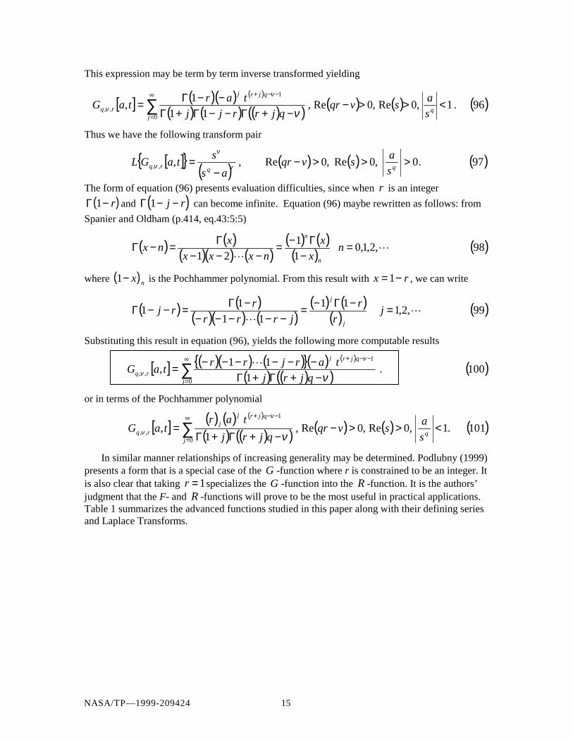
This expression may be term by term inverse transformed yielding
[ ] ( )( ) ( )
( ) ( ) ( )( ) ( ) ( ) ( )96.1,0Re,0Re,11
1,
0
1
,, <>>−−+Γ−−Γ+Γ
−−Γ=∑∞
=
−−+
qj
qjrj
rq s
asvqr
qjrrjj
tartaG
ν
ν
ν
Thus we have the following transform pair
[ ]{ } ( ) ( ) ( ) ( )97.0,0Re,0Re,,,, >>>−−
=qrqrq s
asvqr
as
staGL
ν
ν
The form of equation (96) presents evaluation difficulties, since when r is an integer
( )Γ 1− r and ( )Γ 1− −j r can become infinite. Equation (96) maybe rewritten as follows: from
Spanier and Oldham (p.414, eq.43:5:5)
( ) ( )( )( ) ( )
( ) ( )( ) ( )98,2,1,01
1
21�
�
=−Γ−=
−−−Γ=−Γ n
x
x
nxxx
xnx
n
n
where ( )1− x n is the Pochhammer polynomial. From this result with x r= −1 , we can write
( ) ( )( )( ) ( )
( ) ( )( ) ( )99,2,1
11
11
11 �
�
=−Γ−=−−−−−
−Γ=−−Γ jr
r
jrrr
rrj
j
j
Substituting this result in equation (96), yields the following more computable results
[ ] ( )( ) ( ){ }( ) ( )
( ) ( )( ) ( )100.1
11,
0
1
,, ∑∞
=
−−+
−+Γ+Γ−−−−−−=
j
qjrj
rq qjrj
tarjrrtaG
ν
ν
ν�
or in terms of the Pochhammer polynomial
[ ] ( ) ( ) ( )
( ) ( )( ) ( ) ( ) ( )101.1,0Re,0Re,1
,0
1
,, ∑∞
=
−−+
<>>−−+Γ+Γ
=j
q
qjrjj
rq s
asvqr
qjrj
tartaG
ν
ν
ν
In similar manner relationships of increasing generality may be determined. Podlubny (1999)presents a form that is a special case of the G -function where r is constrained to be an integer. Itis also clear that taking r =1specializes the G -function into the R -function. It is the authors’judgment that the F- and R -functions will prove to be the most useful in practical applications.Table 1 summarizes the advanced functions studied in this paper along with their defining seriesand Laplace Transforms.
NASA/TP—1999-209424
16
SummaryThis paper has presented a new function for use in the fractional calculus, it is called the
R -function. The R -function is unique in that it contains all of the derivatives and integrals ofthe F-function. The R -function has the eigen-property, that is it returns itself on qth order differ-integration. Special cases of the R -function also include the exponential function, the sine,cosine, hyperbolic sine and hyperbolic cosine functions. Further, the R -function contains, asspecial cases; the Mittag-Leffler function, Agarwal's function, Erdelyi's function, Hartley'sF-function, and Miller and Ross's function. Numerous identities are possible with theR -function some of these have been shown in the text.
The value of the R -function is clearly demonstrated in the dynamic thermocouple problemwhere it enables the analyst to directly inverse transform the Laplace domain solution,(operational (s) form) to obtain the time domain solution.
A further generalization of the R -function, called the G -function brings in the effects ofrepeated and partially repeated fractional poles. This generalization carries increased timedomain complexity.
A R -function based trigonometry is also possible. It is a generalization of the conventionaltrigonometry, and will be the subject of a future paper.
Table 1 Summary of Defining Series and Laplace
Function Time Expression Laplace Transform Remarks
Mittag-Leffler [ ] ( )E ata t
nqq
qn nq
n
=+=
∞
∑Γ 10 ( )s
s s a
q
q −( )q−1 differintegral of
Agarwal ( )( )( )
( )E tt
mq
m q
mα β
β α
α β,
/
=+
+ −
=
∞
∑1
0Γs
s
α β
α
−
−1
Erdelyi ( ) ( )E tt
m
m
mα β α β, =
+=
∞
∑Γ0
( )( )∑
∞
=++Γ
+Γ0
1
1
mmsm
mβα
0, >βα
Robotnov / Hartley [ ]( )
( )( )F a ta t
n qq
n n q
n
, =+
+ −
=
∞
∑1 1
0 1Γ1
s aq − eigenfunction
Miller-Ross ( ) ( )E v aa t
v kt
k k v
k
, =+ +
+
=
∞
∑Γ 10
s
s a
v−
−
Current Paper ( )( )
( )( )∑∞
=
−−+
−+Γ=
0
11
,1
,n
vqnn
vqvqn
tataR
s
s a
v
q − eigenfunction & differintegral
Current Paper ( )( ) ( ) ( )( )
( ) ( ) ( )( )G a tr a t
j r j q vq v r
jj r j q v
jj
, , , =−
− + + −
+ − −
=
∞
∑1
0 1 1Γ Γ ( )s
s a
v
q r−eigenfunction & differintegrals
repeated & partially rep.l
NASA/TP—1999-209424

17
ReferencesErdelyi, A., Editor, Magnus, W., Oberhetinger F., and Tricomi F.G., Tables of IntegralTransforms, vol. 1, McGraw-Hill Book Co., 1954, LCC Number 54–6214.
Hartley, T.T. and Lorenzo, C.F., A Solution to the Fundamental Linear Fractional OrderDifferential Equation, NASA /TP—1998-208963, December 1998.
Hartley, T.T. and Lorenzo, C.F., The Vector Linear Fractional Initialization Problem,NASA /TP—1999-208919, May 1999.
Miller, K.S. and Ross, B., An Introduction to the Fractional Calculus and Fractional DifferentialEquations, John Wiley & Sons, Inc., 1993.
Mittag-Leffler, M.G., Une generalisation de l’integrale de Laplace-Abel, Proc. Paris Academy ofScience, pp. 537–539, March 2, 1903(a).
Mittag-Leffler, M.G., Sur la nouvelle fontion ( )xEa , Proc. Paris Academy of Science,
pp. 554–558, October 21, 1903(b).
Mittag-Leffler, M.G., Sur la representation analytique d’une branche uniforme d’une fonctionmonogene, Acta Mathematica, vol. 29, pp. 101–181, 1905.
Podlubny, I., Fractional Order Systems and PI Dλ µ Controllers, IEEE Transactions on AutomaticControl, vol. 44, no. 1, January 1999.
Spanier, J. and Oldham, K.B., An Atlas of Functions, Hemisphere Publishing Corp. (Subsidiaryof Harper & Row, Publishers Inc.) 1987.
Wylie, C.R., Advanced Engineering Mathematics, Fourth Edition, McGraw-Hill Book Co., 1975.
Robotnov, Y.N., Tables of a Fractional Exponential Function of Negative Parameters and ItsIntegral (in Russian), Nauka, Russia (1969).
Robotnov, Y.N., Elements of Hereditary Solid Mechanics (in English) MIR Publishers,Moscow, 1980.
NASA/TP—1999-209424

This publication is available from the NASA Center for AeroSpace Information, (301) 621–0390.
REPORT DOCUMENTATION PAGE
2. REPORT DATE
19. SECURITY CLASSIFICATION OF ABSTRACT
18. SECURITY CLASSIFICATION OF THIS PAGE
Public reporting burden for this collection of information is estimated to average 1 hour per response, including the time for reviewing instructions, searching existing data sources,gathering and maintaining the data needed, and completing and reviewing the collection of information. Send comments regarding this burden estimate or any other aspect of thiscollection of information, including suggestions for reducing this burden, to Washington Headquarters Services, Directorate for Information Operations and Reports, 1215 JeffersonDavis Highway, Suite 1204, Arlington, VA 22202-4302, and to the Office of Management and Budget, Paperwork Reduction Project (0704-0188), Washington, DC 20503.
NSN 7540-01-280-5500 Standard Form 298 (Rev. 2-89)Prescribed by ANSI Std. Z39-18298-102
Form Approved
OMB No. 0704-0188
12b. DISTRIBUTION CODE
8. PERFORMING ORGANIZATION REPORT NUMBER
5. FUNDING NUMBERS
3. REPORT TYPE AND DATES COVERED
4. TITLE AND SUBTITLE
6. AUTHOR(S)
7. PERFORMING ORGANIZATION NAME(S) AND ADDRESS(ES)
11. SUPPLEMENTARY NOTES
12a. DISTRIBUTION/AVAILABILITY STATEMENT
13. ABSTRACT (Maximum 200 words)
14. SUBJECT TERMS
17. SECURITY CLASSIFICATION OF REPORT
16. PRICE CODE
15. NUMBER OF PAGES
20. LIMITATION OF ABSTRACT
Unclassified Unclassified
Technical Paper
Unclassified
National Aeronautics and Space AdministrationJohn H. Glenn Research Center at Lewis FieldCleveland, Ohio 44135–3191
1. AGENCY USE ONLY (Leave blank)
10. SPONSORING/MONITORING AGENCY REPORT NUMBER
9. SPONSORING/MONITORING AGENCY NAME(S) AND ADDRESS(ES)
National Aeronautics and Space AdministrationWashington, DC 20546–0001
October 1999
NASA TP—1999-209424/REV1
E–11944
WU–523–22–13–00
Unclassified -UnlimitedSubject Categories: 59, 66, and 67
23
A03
Generalized Functions for the Fractional Calculus
Carl F. Lorenzo and Tom T. Hartley
Fractional calculus; Fractional differential equations; Systems; Generalized functions;Eigenfunctions
Distribution: Standard
Carl F. Lorenzo, NASA Glenn Research Center, and Tom T. Hartley, The University of Akron, Department of ElectricalEngineering, Akron, Ohio 44325–3904. Responsible person, Carl F. Lorenzo, organization code 5500, (216) 433–3733.
Previous papers have used two important functions for the solution of fractional order differential equations, the Mittag-Leffler function Eq[atq] (1903a, 1903b, 1905), and the F-function Fq[a,t] of Hartley & Lorenzo (1998). These functionsprovided direct solution and important understanding for the fundamental linear fractional order differential equation andfor the related initial value problem (Hartley and Lorenzo, 1999). This paper examines related functions and their Laplacetransforms. Presented for consideration are two generalized functions, the R-function and the G-function, useful inanalysis and as a basis for computation in the fractional calculus. The R-function is unique in that it contains all of thederivatives and integrals of the F-function. The R-function also returns itself on qth order differ-integration. An exampleapplication of the R-function is provided. A further generalization of the R-function, called the G-function brings in theeffects of repeated and partially repeated fractional poles.