
Gene-expression programming for sediment transport in...
23
Accepted Manuscript Not Copyedited 1 Gene-expression programming for sediment transport in sewer pipe systems Aminuddin Ab. Ghani 1 and H. Md. Azamathulla, M.ASCE 2 ________________________________________________________________ Abstract Old sewerage systems were designed based on empirical rules to minimize sediment problems and a list of codes for self-cleansing sewers. These codes were applicable to non- cohesive sediments (typically storm sewers). This study presents gene-expression programming (GEP), which is an extension of genetic programming (GP), as an alternative approach to modeling the functional relationships of sediment transport in sewer pipe systems. A functional relation has been developed using GEP. The proposed relationship can be applied to different boundaries with partial flow. The proposed GEP approach gives satisfactory results (r 2 =0.97 and MSE=0.0054) compared to existing predictor. Key Words: Sewers, Sediment transport, Part-full flow, Gene-expression programming, Regression analysis. ________________________________________________________________________________________________________________ 1 Professor, River Engineering and Urban Drainage Research Centre (REDAC), Universiti Sains Malaysia, Engineering Campus, Seri Ampangan, 14300 Nibong Tebal, Pulau Pinang, Malaysia. Email: [email protected] 2 Senior Lecturer, REDAC, Universiti Sains Malaysia, Engineering Campus, Seri Ampangan, 14300 Nibong Tebal, Pulau Pinang, Malaysia; Email: [email protected] , [email protected] (author for correspondence) Journal of Pipeline Systems Engineering and Practice. Submitted August 3, 2010; accepted December 8, 2010; posted ahead of print December 10, 2010. doi:10.1061/(ASCE)PS.1949-1204.0000076 Copyright 2010 by the American Society of Civil Engineers
Transcript of Gene-expression programming for sediment transport in...

Accep
ted M
anus
cript
Not Cop
yedit
ed
1
Gene-expression programming for sediment transport in sewer pipe systems
Aminuddin Ab. Ghani1
and H. Md. Azamathulla, M.ASCE2
________________________________________________________________
Abstract
Old sewerage systems were designed based on empirical rules to minimize sediment
problems and a list of codes for self-cleansing sewers. These codes were applicable to non-
cohesive sediments (typically storm sewers). This study presents gene-expression
programming (GEP), which is an extension of genetic programming (GP), as an alternative
approach to modeling the functional relationships of sediment transport in sewer pipe
systems. A functional relation has been developed using GEP. The proposed relationship can
be applied to different boundaries with partial flow. The proposed GEP approach gives
satisfactory results (r2=0.97 and MSE=0.0054) compared to existing predictor.
Key Words: Sewers, Sediment transport, Part-full flow, Gene-expression programming,
Regression analysis.
________________________________________________________________________________________________________________
1Professor, River Engineering and Urban Drainage Research Centre (REDAC), Universiti
Sains Malaysia, Engineering Campus, Seri Ampangan, 14300 Nibong Tebal, Pulau Pinang,
Malaysia. Email: [email protected]
2Senior Lecturer, REDAC, Universiti Sains Malaysia, Engineering Campus, Seri Ampangan,
14300 Nibong Tebal, Pulau Pinang, Malaysia; Email: [email protected],
[email protected] (author for correspondence)
Journal of Pipeline Systems Engineering and Practice. Submitted August 3, 2010; accepted December 8, 2010; posted ahead of print December 10, 2010. doi:10.1061/(ASCE)PS.1949-1204.0000076
Copyright 2010 by the American Society of Civil Engineers

Accep
ted M
anus
cript
Not Cop
yedit
ed
2
Introduction
In sewer networks, the deposition of solids occurs occasionally due to the intermittent nature
of flow (Nalluri et al., 1994). The longer the deposits remain in the sewer the more likely that
the sediment properties change and can eventually become consolidated or cemented,
especially during dry weather flows. Such permanent deposits in pipe inverts will change the
nature of the velocity and boundary shear distributions, which affects the sediment carrying
capacity and hydraulic resistance of sewers. Previous work on sediment transport with no
deposition includes that by Novak and Nalluri (1975, 1984), May et al. (1996), Mayerle et al.
(1991) and Vongvisessomjai et al., 2010.
Sewer system designs must satisfy two major criteria: high flow and low flow criteria. During
high flows, sewer systems must convey the design discharge. For low flows, sewers should
be free from sediment deposit as much as possible. Traditionally, a fixed minimum flow
velocity for non-deposition, such as 0.6 m/s (ASCE 1970) is used as a low flow criterion.
This criterion may be inadequate because the loading and sediment characteristics vary
considerably under different environmental conditions (Vongvisessomjai et al., 2010).
The present study investigates the hydraulic characteristics of the flow in channels with a
circular cross-section with different bed roughness and their effects on sediment transport
capacity (Figure 1) (Nalluri and Ab. Ghani, 1996). The pipe channel can be represented by a
trapezoidal section, especially at low depths; at high depths, the cross-section is influenced by
the „crowing‟ effect of the pipe, through the changes in velocity and shear distributions due to
changes in cross-sectional shapes (Nalluri et al., 1994).
Journal of Pipeline Systems Engineering and Practice. Submitted August 3, 2010; accepted December 8, 2010; posted ahead of print December 10, 2010. doi:10.1061/(ASCE)PS.1949-1204.0000076
Copyright 2010 by the American Society of Civil Engineers
Accep
ted M
anus
cript
Not Cop
yedit
ed
3
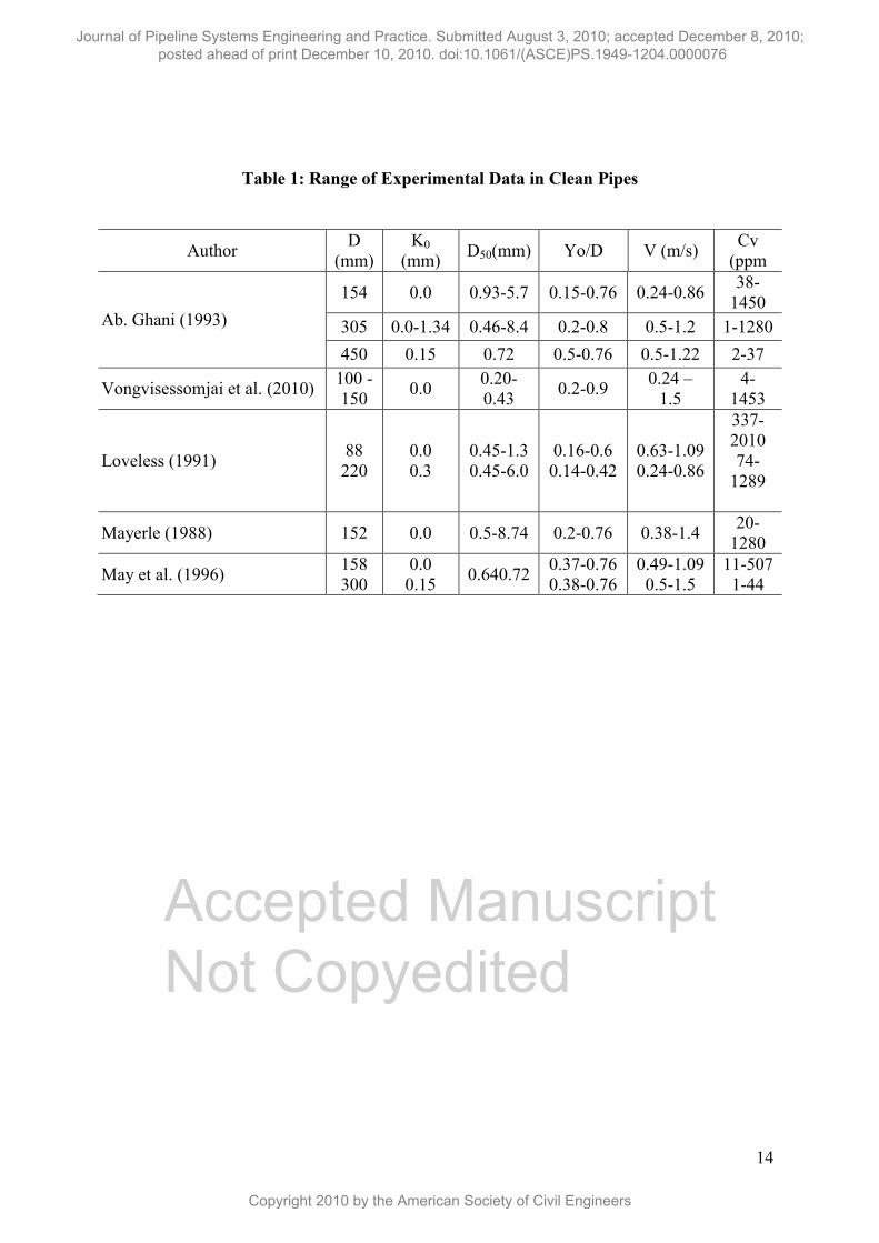
Extensive experimental work (Ab. Ghani 1993; Nalluri and Ab. Ghani 1994a, b) on bed load
transport of non-cohesive sediments with no deposition (Fig. 2) was carried out in pipe
channels with diameters of 154 mm, 305 mm, and 450 mm covering a wide range of flow
depths, sediment sizes and three different bed roughness values, as shown in Table 1. The
limiting sediment concentrations Cv(=Qs/Q) for the „no deposition‟ criterion with uniform
flow conditions were established for several flow depths (yo) over each bed roughness.
Multiple Linear Regression - Clean Pipes
The sediment transport rate in channels with a circular cross section or pipe channels depends
on many factors, such as flow depth (yo), bed slope (So), sediment size (d50), density of
sediment (ρs), kinematic viscosity (ν) and density (ρ ) of fluid, friction factor (λ), pipe
diameter (D), and gravitational constant (g).
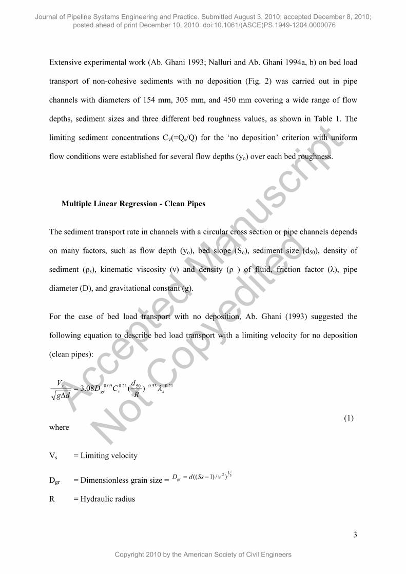
For the case of bed load transport with no deposition, Ab. Ghani (1993) suggested the
following equation to describe bed load transport with a limiting velocity for no deposition
(clean pipes):
21.053.05021.009.0 )(08.3
svgr
s
R
dCD
dg
V
(1)
where
Vs = Limiting velocity
Dgr = Dimensionless grain size = 3
12 )/)1(( SsdDgr
R = Hydraulic radius
Journal of Pipeline Systems Engineering and Practice. Submitted August 3, 2010; accepted December 8, 2010; posted ahead of print December 10, 2010. doi:10.1061/(ASCE)PS.1949-1204.0000076
Copyright 2010 by the American Society of Civil Engineers
Accep
ted M
anus
cript
Not Cop
yedit
ed
4
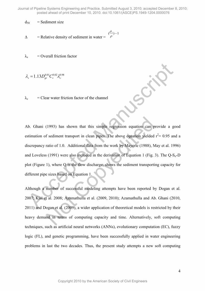
d50 = Sediment size
∆ = Relative density of sediment in water = 1)(
s
λs = Overall friction factor
98.002.001.013.1 cvgrs CD
λc = Clear water friction factor of the channel
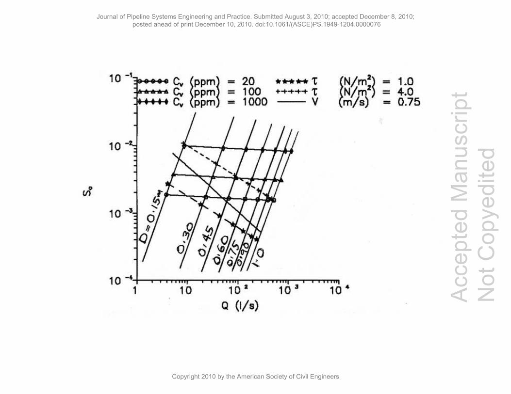
Ab. Ghani (1993) has shown that this simple regression equation can provide a good
estimation of sediment transport in clean pipes. The above equation yielded r2= 0.95 and a
discrepancy ratio of 1.0. Additional data from the work by Mayerle (1988), May et al. 1996)
and Loveless (1991) were also included in the derivation of Equation 1 (Fig. 3). The Q-So-D
plot (Figure 1), where Q is the flow discharge, shows the sediment transporting capacity for
different pipe sizes based on Equation 1.
Although a number of successful modeling attempts have been reported by Dogan et al.
2007; Kisi et al. 2008; Azamathulla et al. (2009, 2010); Azamathulla and Ab. Ghani (2010,
2011) and Dogan et al. (2009), a wider application of theoretical models is restricted by their
heavy demand in terms of computing capacity and time. Alternatively, soft computing
techniques, such as artificial neural networks (ANNs), evolutionary computation (EC), fuzzy
logic (FL), and genetic programming, have been successfully applied in water engineering
problems in last the two decades. Thus, the present study attempts a new soft computing
Journal of Pipeline Systems Engineering and Practice. Submitted August 3, 2010; accepted December 8, 2010; posted ahead of print December 10, 2010. doi:10.1061/(ASCE)PS.1949-1204.0000076
Copyright 2010 by the American Society of Civil Engineers

Accep
ted M
anus
cript
Not Cop
yedit
ed
5
technique, GEP, to obtain a new sediment transport equation for bed load transport in pipes
with no deposition
Overview of GEP
GEP, which is an extension of GP (Koza, 1992), is a search technique that involves computer
programs (e.g., mathematical expressions, decision trees, polynomial constructs, and logical
expressions). GEP computer programs are all encoded in linear chromosomes, which are then
expressed or translated into expression trees (ETs). ETs are sophisticated computer programs
that have usually evolved to solve a particular problem and are selected according to their
fitness at solving that problem.
GEP is a full-fledged genotype/phenotype system, with the genotype totally separated
from the phenotype, whereas in GP, genotype and phenotype are mixed together in a simple
replicator system. As a result, the full-fledged genotype/phenotype system of GEP surpasses
the old GP system by a factor of 100-60,000 (Ferreira 2001a, b).
Initially, the chromosomes of each individual in the population are generated randomly.
Then, the chromosomes are expressed, and each individual is evaluated based on a fitness
function and selected to reproduce with modification, leaving progeny with new traits. The
individuals in the new generation are, in their turn, subjected to some developmental
processes, such as expression of the genomes, confrontation of the selection environment,
and reproduction with modification. These processes are repeated for a predefined number of
generations or until a solution is achieved (Ferreira 2001a, b). The functionality of each
genetic operator included in GEP system has been explained by Guven and Aytek (2009).
Journal of Pipeline Systems Engineering and Practice. Submitted August 3, 2010; accepted December 8, 2010; posted ahead of print December 10, 2010. doi:10.1061/(ASCE)PS.1949-1204.0000076
Copyright 2010 by the American Society of Civil Engineers

Accep
ted M
anus
cript
Not Cop
yedit
ed
6
Derivation of Froude Number based on GEP
In this section, the sediment load is modeled using the GEP approach. Initially, the “training
set” is selected from the entire data set, and the rest is used as the “testing set”. Once the
training set is selected, one could say that the learning environment of the system is defined.
The modeling also includes five major steps to prepare to use GEP. The first is to choose the
fitness function. For this problem, the fitness, fi, of an individual program, i, is measured by:
tC
jjjii TCMf
1),(
(2)
where M is the range of selection, C(i,j) is the value returned by the individual chromosome i
for fitness case j (out of Ct fitness cases) and Tj is the target value for fitness case j. If |C(i,j) -
Tj| (the precision) ≦ 0.01, then the precision is 0, and fi = fmax = CtM. In this case, M = 100 is
used; therefore, fmax = 1000. The advantage of this kind of fitness function is that the system
can find the optimal solution by itself.
Secondly, the set of terminals T and the set of functions F are chosen to create the
chromosomes. In this problem, the terminal set consists of single independent variable, i.e., T
= {h}. The choice of the appropriate function set is not so clear; however, a good guess is
helpful if it includes all the necessary functions. In this study, four basic arithmetic operators
(+, -, *, /) and some basic mathematical functions (√) are utilized.
The third major step is to choose the chromosomal architecture, i.e., the length of the
head and the number of genes. We initially used single gene and two head lengths and
increased the number of genes and heads one at a time during each run while we monitored
the training and testing performances of each model. We observed that more than two genes
more and a head length greater than 8 did not significantly improve the training and testing
Journal of Pipeline Systems Engineering and Practice. Submitted August 3, 2010; accepted December 8, 2010; posted ahead of print December 10, 2010. doi:10.1061/(ASCE)PS.1949-1204.0000076
Copyright 2010 by the American Society of Civil Engineers

Accep
ted M
anus
cript
Not Cop
yedit
ed
7
performance of GEP models. Thus, the head length, lh = 8, and two genes per chromosome
are employed for each GEP model in this study.
The fourth major step is to choose the linking function. In this study, addition and
multiplication operators are used as linking functions, and it is observed that linking the sub-
ETs by addition gives better fitness (Eq. 2) values. The fifth and final step is to choose the set
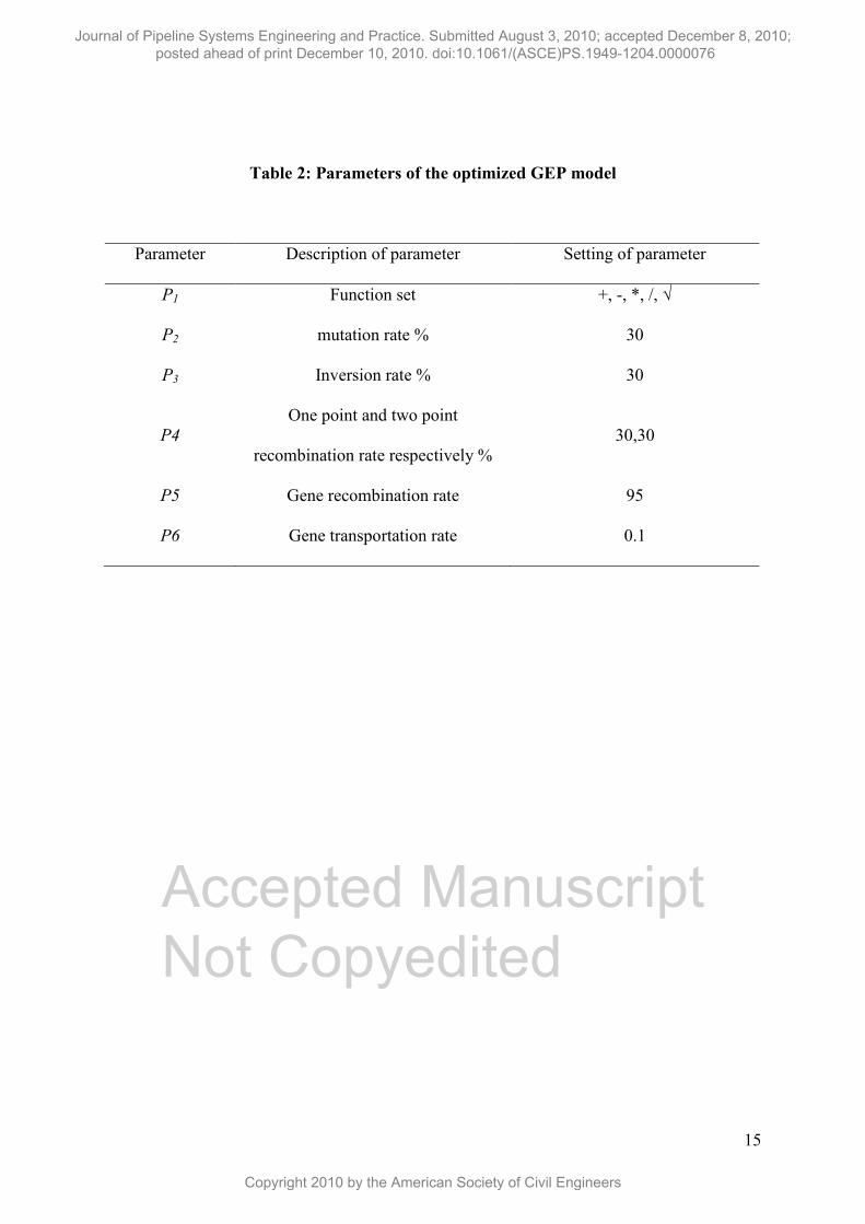
of genetic operators that cause variation and their rates. A combination of all genetic
operators (mutation, transposition and crossover) is used for this purpose (Table 2).
Table 3 compares the GEP model with one of the independent parameters removed in
each case and any independent parameter from the input set that yielded larger RMSE and
lower R2 values also removed. These five independent parameters affect Fr =
dg
Vs
; thus, the
functional relationship given in Eq. (1) is used for the GEP model in this study. The GEP
approach resulted in a highly nonlinear relationship between dg
Vs
and the input
parameters, and the GEP model had the highest accuracy and the lowest error (Table 3).
The GEP model was calibrated with 220 input-target pairs of collected data by Ab. Ghani
(1993) and Vongvisessomjai et al., 2010. Among the 220 data sets, 55 (25%) were reserved
for validation (testing), and the remaining 165 sets were used to calibrate the GP model.
The best individual in each generation has 30 chromosomes has and a fitness 780.5
fordg
Vs
. The explicit formulations of GEP for
dg
Vs
are given in Eq. (3), and the
corresponding expression trees are shown in Fig. 4.
Journal of Pipeline Systems Engineering and Practice. Submitted August 3, 2010; accepted December 8, 2010; posted ahead of print December 10, 2010. doi:10.1061/(ASCE)PS.1949-1204.0000076
Copyright 2010 by the American Society of Civil Engineers
Accep
ted M
anus
cript
Not Cop
yedit
ed
8
)34.8(
)(91.5
91.5
014.0411.0
41.0
014.0 sd
RsDs
D
C
d
Rd
R
dg
Vgr
s
gr
sVS
s
s
(3)
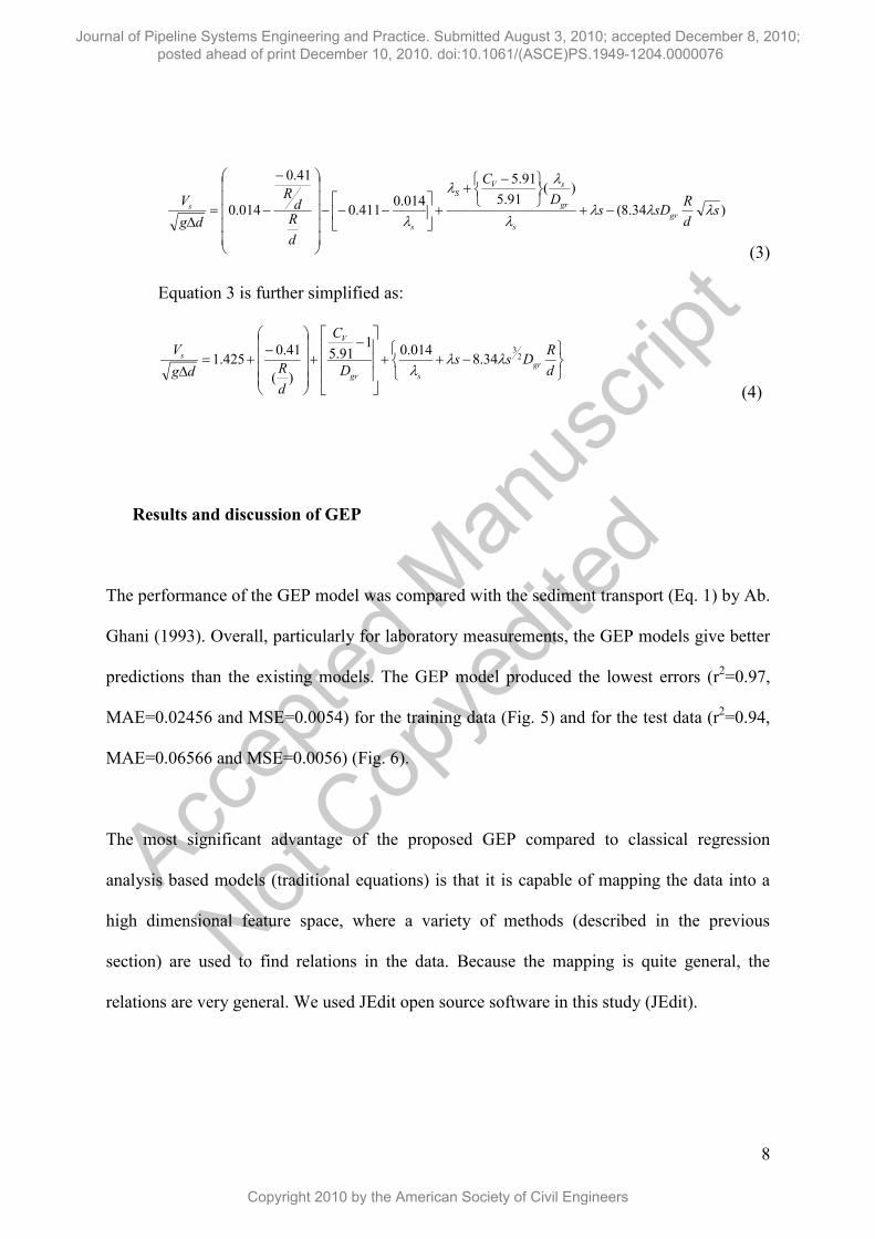
Equation 3 is further simplified as:
d
RDss
D
C
d
Rdg
Vgr
sgr
V
s 23
34.8014.0
191.5
)(
41.0425.1
(4)
Results and discussion of GEP
The performance of the GEP model was compared with the sediment transport (Eq. 1) by Ab.
Ghani (1993). Overall, particularly for laboratory measurements, the GEP models give better
predictions than the existing models. The GEP model produced the lowest errors (r2=0.97,
MAE=0.02456 and MSE=0.0054) for the training data (Fig. 5) and for the test data (r2=0.94,
MAE=0.06566 and MSE=0.0056) (Fig. 6).
The most significant advantage of the proposed GEP compared to classical regression
analysis based models (traditional equations) is that it is capable of mapping the data into a
high dimensional feature space, where a variety of methods (described in the previous
section) are used to find relations in the data. Because the mapping is quite general, the
relations are very general. We used JEdit open source software in this study (JEdit).
Journal of Pipeline Systems Engineering and Practice. Submitted August 3, 2010; accepted December 8, 2010; posted ahead of print December 10, 2010. doi:10.1061/(ASCE)PS.1949-1204.0000076
Copyright 2010 by the American Society of Civil Engineers
Accep
ted M
anus
cript
Not Cop
yedit
ed
9
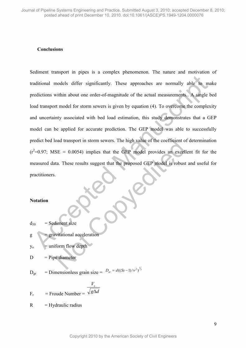
Conclusions
Sediment transport in pipes is a complex phenomenon. The nature and motivation of
traditional models differ significantly. These approaches are normally able to make
predictions within about one order-of-magnitude of the actual measurements.. A single bed
load transport model for storm sewers is given by equation (4). To overcome the complexity
and uncertainty associated with bed load estimation, this study demonstrates that a GEP
model can be applied for accurate prediction. The GEP model was able to successfully
predict bed load transport in storm sewers. The high value of the coefficient of determination
(r2=0.97; MSE = 0.0054) implies that the GEP model provides an excellent fit for the
measured data. These results suggest that the proposed GEP model is robust and useful for
practitioners.
Notation
d50 = Sediment size
g = gravitational acceleration
yo = uniform flow depth
D = Pipe diameter
Dgr = Dimensionless grain size = 3
12 )/)1(( SsdDgr
Fr = Froude Number = dg
Vs
R = Hydraulic radius
Journal of Pipeline Systems Engineering and Practice. Submitted August 3, 2010; accepted December 8, 2010; posted ahead of print December 10, 2010. doi:10.1061/(ASCE)PS.1949-1204.0000076
Copyright 2010 by the American Society of Civil Engineers
Accep
ted M
anus
cript
Not Cop
yedit
ed
10
Vs = Limiting velocity
r2 = coefficient of determination
MAE = mean average error
∆ = Relative density of sediment in water =
λs = Overall friction factor
λc = Clear water friction factor of the channel
= fluid density
s = buoyant sediment density
References
Ab. Ghani, A., (1993). Sediment transport in sewers. PhD. Thesis, University of Newcastle
upon Tyne, UK.
American Society of Civil Engineers (ASCE)(1970). Water pollution control federation,
Design and construction of sanitary and storm sewers. American Society of Civil
Engineers Manuals and Reports on Engineering Practices, No. 37.
Azamathulla, H. Md, Ab. Ghani, A. Zakaria, N. A. and Guven, A., (2010). Genetic
programming to predict bridge pier scour. ASCE Journal of Hydraulic Engineering, 2010;
136(3),165-169.
Azamathullah, H.Md., Chang, C.K. Ab Ghani, A., Ariffin, J., Zakaria, N.A., and Abu Hasan,
Z., (2009). An ANFIS-Based Approach for Predicting the Bed Load for Moderately-
Sized Rivers. Journal of Hydro-Environment Research, IAHR, Vol. 3, No. 1, pp. 35-44.
Azamathulla, H. MD. and Ab. Ghani, A., (2010). Genetic programming to predict river
pipeline scour, ASCE, Journal of Pipeline system and Engineering Practice. 1(3)127-132.
Journal of Pipeline Systems Engineering and Practice. Submitted August 3, 2010; accepted December 8, 2010; posted ahead of print December 10, 2010. doi:10.1061/(ASCE)PS.1949-1204.0000076
Copyright 2010 by the American Society of Civil Engineers

Accep
ted M
anus
cript
Not Cop
yedit
ed
11
Azamathulla, H. MD. and Ab. Ghani, A., (2011). An ANFIS-based approach for predicting
the scour depth at culvert outlet, ASCE, Journal of Pipeline system and Engineering
Practice. (In press).
Bhattacharya, B., Price, R.K., and Solomatine, D,P., (2007). Machine Learning Approach to
Modeling Sediment Transport, ASCE Journal of Hydraulic Engineering, 2007, 133(4),
440-450.
Department of Irrigation and Drainage Malaysia or DID., (2009). Study on River Sand
Mining Capacity in Malaysia.
Dogan, E., Yuksel, I. and Kisi, O., (2007). Estimation of Sediment Concentration Obtained
by Experimental Study Using Artificial Neural Networks, Environmental Fluid
Mechanics, 7, 271-288.
Dogan, E., Tripathi, S., Lyn, D. A and Govindaraju, R. S., (2009). From flumes to rivers: Can
sediment transport in natural alluvial channels be predicted from observations at the
laboratory scale?, Water Resour. Res., 114, W08433, doi:10.1029/2008WR007637.
Engelund F. and Hansen.E., (1967). A monograph on sediment transport in alluvial streams,
Teknisk Forlag, Copenhagen, Denmark.
Ferreira, C., (2001a). Gene expression programming in problem solving, 6th
Online World
Conference on Soft Computing in Industrial Applications (invited tutorial).
Ferreira, C. (2001b). Gene expression programming: A new adaptive algorithm for solving
problems. Complex Systems, 13 (2), 87–129.
Guven, A. and Gunal, M., (2008a). Prediction of scour downstream of grade-control
structures using neural networks.ASCE Journal of Hydraulic Engineering, 134(11),
1656-1660.
Journal of Pipeline Systems Engineering and Practice. Submitted August 3, 2010; accepted December 8, 2010; posted ahead of print December 10, 2010. doi:10.1061/(ASCE)PS.1949-1204.0000076
Copyright 2010 by the American Society of Civil Engineers

Accep
ted M
anus
cript
Not Cop
yedit
ed
12
Guven, A. and Gunal, M., (2008b). Genetic programming for prediction of local scour
downstream of grade-control structures. ASCE Journal of Irrigation and Drainage
Engineering, 134(2), 241-249.
Guven, A. and Aytek, A.. (2009). A new approach for stage-discharge relationship: Gene-
Expression Programming, J. Hydrologic Engineering, 14(8),812-820.
Holland, J. H. (1975). Adaptation in natural and artificial system. University of Michigan
Press, Ann Arbor, Mich.
JEdit, http://sourceforge.net/projects/jedit/
Kisi, O, Yuksel, I. and Dogan, E., (2008). Modelling daily suspended sediment of rivers in
Turkey using several data driven techniques, Hydrol. Sci. J., 53(6), 1270-1285.
Koza, J.R., (1999). Genetic Programming: On the Programming of Computers by means of
Natural Selection. The MIT Press, Cambridge, MA.
Keijzer, M., and Babovic, V., (2002). Declarative and preferential bias in GP-based scientific
discovery. Genetic Programming and Evolvable Machines, 1(3), 41-79.
Kizhisseri, A.S., Simmonds, D., Rafiq, Y., and Borthwick, M., (2005). An evolutionary
computation approach to sediment transport modeling. In: Fifth International Conference
on Coastal Dynamics, April 4–8, 2005, Barcelona, Spain.
Loveless, J. H.,( 1991). Sediment transport in rigid boundary channels with particular
reference to the condition of incipeint deposition. PhD thesis , Univeristy of London,
U.K.
Mayerle, R., (1988). Sediment transport in rigid boundary channel. PhD Thesis, University of
Newcastle upon Tyne, UK.
Mayerle, R., Nalluri, C., and Novak, P., (1991). Sediment transport in rigid bed conveyances.
Journal of Hydraulic Research, 29 (4), 475–496.
Journal of Pipeline Systems Engineering and Practice. Submitted August 3, 2010; accepted December 8, 2010; posted ahead of print December 10, 2010. doi:10.1061/(ASCE)PS.1949-1204.0000076
Copyright 2010 by the American Society of Civil Engineers

Accep
ted M
anus
cript
Not Cop
yedit
ed
13
May, R.W.P., Ackers, J.C., Butler, D. and John, S., (1996). Development of design
methodology for self-cleansing sewers. Water Science and Technology, 33 (9), 195–205.
Nalluri, C., Ghani, A.A., and El-Zaemey, A.K.S., (1994). Sediment transport over deposited
beds in sewers. Water Science and Technology, 29 (1–2), 125–133.
Nalluri, C. & Ab. Ghani, A., (1994). Sediment Transport in Sewers and Design Implications.
National Conference on Hydraulic Engineering; Hydraulic Division, ASCE, Buffalo,
USA, Vol. 2, pp. 933-938, 1 - 5 August.
Nalluri, C. & Ab. Ghani, A., (1994). Sediment Transport in Sewers with and without
Deposited Beds. 9th Congress of Asia-Pacific Division of IAHR, Singapore, Vol. 2, pp.
27-34, 24 - 26 August.
Nalluri, C. and Ab. Ghani, A., (1996). Design Options For Self-Cleansing Storm Sewers.
Journal of Water Science and Technology, IWA, Vol. 33, No. 9, pp. 215-220.
Oltean, M., and Groşan, C,, (2003). A comparison of several linear genetic programming
techniques. Complex Systems, 14(1), 1-29.
Solomatine, D.P. and Otsfeld, A., (2008). Data-driven modelling: some past experiences and
new approaches. Journal of Hydroinformatics, 2008, 10, No. 1, 3-22.
Vongvisessomjai, N., Tingsanchali, T. and Babel, M. S., (2010). Non-deposition design
criteria for sewers with part-full flow, Urban Water Journal, 7(1), 61-77.
Journal of Pipeline Systems Engineering and Practice. Submitted August 3, 2010; accepted December 8, 2010; posted ahead of print December 10, 2010. doi:10.1061/(ASCE)PS.1949-1204.0000076
Copyright 2010 by the American Society of Civil Engineers
14
Table 1: Range of Experimental Data in Clean Pipes
Author D
(mm)
K0
(mm) D50(mm) Yo/D V (m/s)
Cv
(ppm
Ab. Ghani (1993)
154 0.0 0.93-5.7 0.15-0.76 0.24-0.86 38-
1450
305 0.0-1.34 0.46-8.4 0.2-0.8 0.5-1.2 1-1280
450 0.15 0.72 0.5-0.76 0.5-1.22 2-37
Vongvisessomjai et al. (2010) 100 -
150 0.0
0.20-
0.43 0.2-0.9
0.24 –
1.5
4-
1453
Loveless (1991) 88
220
0.0
0.3
0.45-1.3
0.45-6.0
0.16-0.6
0.14-0.42
0.63-1.09
0.24-0.86
337-
2010
74-
1289
Mayerle (1988) 152 0.0 0.5-8.74 0.2-0.76 0.38-1.4 20-
1280
May et al. (1996) 158
300
0.0
0.15 0.640.72
0.37-0.76
0.38-0.76
0.49-1.09
0.5-1.5
11-507
1-44
Accepted Manuscript Not Copyedited
Journal of Pipeline Systems Engineering and Practice. Submitted August 3, 2010; accepted December 8, 2010; posted ahead of print December 10, 2010. doi:10.1061/(ASCE)PS.1949-1204.0000076
Copyright 2010 by the American Society of Civil Engineers
15
Table 2: Parameters of the optimized GEP model
Parameter Description of parameter Setting of parameter
P1 Function set +, -, *, /, √
P2 mutation rate % 30
P3 Inversion rate % 30
P4
One point and two point
recombination rate respectively %
30,30
P5 Gene recombination rate 95
P6 Gene transportation rate 0.1
Accepted Manuscript Not Copyedited
Journal of Pipeline Systems Engineering and Practice. Submitted August 3, 2010; accepted December 8, 2010; posted ahead of print December 10, 2010. doi:10.1061/(ASCE)PS.1949-1204.0000076
Copyright 2010 by the American Society of Civil Engineers

16
Table 3. Sensitivity Analysis for Independent Parameters for the Testing
Set Model MSE MAE
r2
),,,( 50svgr
s
R
dCDf
dg
V
0.0056 0.65 0.94
),,( 50sv
s
R
dCf
dg
V
0.099 0.88 0.86
),,( 50sgr
s
R
dDf
dg
V
0.094 0.95 0.79
),,( svgrs CDfdg
V
0.109 0.85 0.76
),,( 50
R
dCDf
dg
Vvgr
s
0.38 0.91 0.78
Accepted Manuscript Not Copyedited
Journal of Pipeline Systems Engineering and Practice. Submitted August 3, 2010; accepted December 8, 2010; posted ahead of print December 10, 2010. doi:10.1061/(ASCE)PS.1949-1204.0000076
Copyright 2010 by the American Society of Civil Engineers

Accep
ted M
anus
cript
Not Cop
yedit
ed
17
List of Figures:
Fig. 1: Q-S0-D plot: clean pipe (Ab. Ghani, 1993)
Fig. 2: Cross section of clean pipes (Ab. Ghani, 1993)
Fig. 3: Limiting velocity criteria for clean pipes (Ab Ghani, 1993)
Fig. 4: Expression Tree (ET) for GEP formulation
Fig. 5: Observed versus predicted sediment load by GEP for partially full pipe flow –
Training data
Fig. 6: Observed versus predicted sediment load by GEP for partially full pipe flow – Test
data
Journal of Pipeline Systems Engineering and Practice. Submitted August 3, 2010; accepted December 8, 2010; posted ahead of print December 10, 2010. doi:10.1061/(ASCE)PS.1949-1204.0000076
Copyright 2010 by the American Society of Civil Engineers
Acc
epte
d M
anus
crip
t N
ot C
opye
dite
d
Journal of Pipeline Systems Engineering and Practice. Submitted August 3, 2010; accepted December 8, 2010; posted ahead of print December 10, 2010. doi:10.1061/(ASCE)PS.1949-1204.0000076
Copyright 2010 by the American Society of Civil Engineers

Acc
epte
d M
anus
crip
t N
ot C
opye
dite
d
Journal of Pipeline Systems Engineering and Practice. Submitted August 3, 2010; accepted December 8, 2010; posted ahead of print December 10, 2010. doi:10.1061/(ASCE)PS.1949-1204.0000076
Copyright 2010 by the American Society of Civil Engineers

Acc
epte
d M
anus
crip
t N
ot C
opye
dite
d
Journal of Pipeline Systems Engineering and Practice. Submitted August 3, 2010; accepted December 8, 2010; posted ahead of print December 10, 2010. doi:10.1061/(ASCE)PS.1949-1204.0000076
Copyright 2010 by the American Society of Civil Engineers

Acc
epte
d M
anus
crip
t N
ot C
opye
dite
d
Journal of Pipeline Systems Engineering and Practice. Submitted August 3, 2010; accepted December 8, 2010; posted ahead of print December 10, 2010. doi:10.1061/(ASCE)PS.1949-1204.0000076
Copyright 2010 by the American Society of Civil Engineers

Acc
epte
d M
anus
crip
t N
ot C
opye
dite
d
Journal of Pipeline Systems Engineering and Practice. Submitted August 3, 2010; accepted December 8, 2010; posted ahead of print December 10, 2010. doi:10.1061/(ASCE)PS.1949-1204.0000076
Copyright 2010 by the American Society of Civil Engineers

Acc
epte
d M
anus
crip
t N
ot C
opye
dite
d
Journal of Pipeline Systems Engineering and Practice. Submitted August 3, 2010; accepted December 8, 2010; posted ahead of print December 10, 2010. doi:10.1061/(ASCE)PS.1949-1204.0000076
Copyright 2010 by the American Society of Civil Engineers