
Futures And Spot Commodity Prices, Options, And Forward ... · Di erent traders have di erent...
209
Futures And Spot Commodity Prices, Options, And Forward interest rates: Model And Empirical Analysis YU MIAO (B.Sc., NANJING UNIVERSITY) A THESIS SUBMITTED FOR THE DEGREE OF DOCTOR OF PHILOSOPHY DEPARTMENT OF PHYSICS NATIONAL UNIVERSITY OF SINGAPORE 2017 Supervisor: Dr. Wang Qinghai Examiners: Professor. Wang Jiansheng Associate Professor. Tan Mengchwan Professor. Emmanuel Haven, Memorial University of Newfoundland
Transcript of Futures And Spot Commodity Prices, Options, And Forward ... · Di erent traders have di erent...

Futures And Spot Commodity Prices,
Options, And Forward interest rates:
Model And Empirical Analysis
YU MIAO
(B.Sc., NANJING UNIVERSITY)
A THESIS SUBMITTED
FOR THE DEGREE OF DOCTOR OF PHILOSOPHY
DEPARTMENT OF PHYSICS
NATIONAL UNIVERSITY OF SINGAPORE
2017
Supervisor:
Dr. Wang Qinghai
Examiners:
Professor. Wang Jiansheng
Associate Professor. Tan Mengchwan
Professor. Emmanuel Haven, Memorial University of
Newfoundland


Declaration
I hereby declare that the thesis is my original work and it has been written by me in its
entirety. I have duly acknowledged all the sources which have been used in the thesis.
This thesis has also not been submitted for any degree in any university previously.
YU MIAO
JULY 2017
i


Acknowledgements
I would like to thank all people who have supported me during my graduate study.
First and foremost, I would like to express my sincerest gratitude and greatest respect to
Professor Belal E Baaquie and my supervisor Dr. Wang Qinghai. My main work is under
the guidance of Professor Baaquie. Without his encouragement, supervision, and support,
the dissertation is definitely not possible. His deep and distinctive view of quantum physics
guided me to think of the world in the language of quantum field theory. Besides the research
field, the opinion and experiences for the life that he shares with me will affect my whole life.
I thank my supervisor Dr. Wang Qinghai for vast advices and guidance for my research and
my PhD thesis.
My sincere thanks also goes to Du Xin, Jiten Bhanap, and Cao Yang for their useful
discussion and collaboration. I thank National University of Singapore and Department of
Physics for the financial support.
Last but not least, I would like to thank my parents, my father Yu Jianxin and my mother
Yu Xiuying, and my wife Tian Maoshan for their unconditional support and precious love.
iii


Summary
Financial market is a platform to improve the efficiency and convenience for all traders in the
world. Different traders have different purposes for their trading and there are three main
types of traders including hedgers, speculators and arbitrageurs, due to three vital purposes.
Whether you aim to hedge, speculate or arbitrage in the market, quantitative analysis is a
strong tool to help you make a better decision. Although recent quantitative study using
statistics and stochastic process as the basic method has already made huge achievements in
financial domain, there are still great numbers of unsolved financial fields which may require
new theories to fill in. In this thesis, quantum field theory is chosen as a new method to analyse
financial instruments. In Chapter 2, a new correlation factor among different commodities
is defined by a new microeconomics theory based on quantum field theory. In Chapter 3,
a new theory of commodity futures with two-Dimension quantum field is proposed and the
theory may fill the gap of the futures theory for financial market. In Chapter 4, an indicator is
designed by comparing option pricing with stochastic method and quantum method to reflect
the market instability. In Chapter 5, a new theory of pricing bond option is raised up to give
contract makers a better reference to price the bond option contract.
v

vi
Publication List
[1] B.E. Baaquie, Miao Yu∗, and Xin Du. ”Multiple Commodities in Statistical Microe-
conomics: Model and Market.” Physica A: Statistical Mechanics and its Applications 462
(2016): 912-929.
[2] B.E. Baaquie and Miao Yu∗. Statistical Field Theory of Futures Commodity Prices.
Submitting paper.
[3] B.E. Baaquie, Miao Yu∗. ”Option Price and Market Instability.” Physica A: Statistical
Mechanics and its Applications 471 (2017): 512-535.
[4] B.E. Baaquie, Miao Yu∗ and Jitendra Bhanap. Risky Forward Interest Rates and
Swaptions: Quantum Finance Model and Empirical Results. Submitting paper.
* Corresponding author
Contents
Declaration i
Acknowledgements iii
Summary v
List of Tables xiv
List of Figures xxi
List of Symbols xxii
1 Introduction 1
§ 1.1 Review of financial market and financial modeling . . . . . . . . . . . . . . . . 1
§ 1.2 Introduction of financial instrument . . . . . . . . . . . . . . . . . . . . . . . . 3
§ 1.2.1 Commodity price and Futures . . . . . . . . . . . . . . . . . . . . . . . 3
§ 1.2.2 Option price . . . . . . . . . . . . . . . . . . . . . . . . . . . . . . . . . 4
§ 1.2.3 Interest rate . . . . . . . . . . . . . . . . . . . . . . . . . . . . . . . . . 6
vii
CONTENTS viii
§ 1.2.4 Bond . . . . . . . . . . . . . . . . . . . . . . . . . . . . . . . . . . . . . 6
§ 1.2.5 One type of swaption: bond option . . . . . . . . . . . . . . . . . . . . 7
§ 1.3 Introduction of financial models . . . . . . . . . . . . . . . . . . . . . . . . . . . 8
§ 1.3.1 Lagrangian model based on supply and demand . . . . . . . . . . . . . 8
§ 1.3.2 Black-Scholes model for option pricing . . . . . . . . . . . . . . . . . . 10
§ 1.3.3 HJM Model for forward interest rate . . . . . . . . . . . . . . . . . . . 12
2 Multiple Commodities in Statistical Microeconomics: Model and Market 14
§ 2.1 Introduction . . . . . . . . . . . . . . . . . . . . . . . . . . . . . . . . . . . . . 14
§ 2.2 The microeconomic action functional . . . . . . . . . . . . . . . . . . . . . . . . 16
§ 2.3 Correlation Function . . . . . . . . . . . . . . . . . . . . . . . . . . . . . . . . . 20
§ 2.3.1 Expansion of Potential . . . . . . . . . . . . . . . . . . . . . . . . . . . 21
§ 2.3.2 Auto-correlation . . . . . . . . . . . . . . . . . . . . . . . . . . . . . . . 22
§ 2.3.3 Cross-correlation . . . . . . . . . . . . . . . . . . . . . . . . . . . . . . 24
§ 2.3.4 Nonlinear terms . . . . . . . . . . . . . . . . . . . . . . . . . . . . . . . 25
§ 2.4 Market data and model . . . . . . . . . . . . . . . . . . . . . . . . . . . . . . . 26
§ 2.5 Fitting with Market Data . . . . . . . . . . . . . . . . . . . . . . . . . . . . . . 28
§ 2.6 Fits for GII , GIJ . . . . . . . . . . . . . . . . . . . . . . . . . . . . . . . . . . . 33
§ 2.6.1 Two commodities . . . . . . . . . . . . . . . . . . . . . . . . . . . . . . 33
§ 2.6.2 Three commodities fit . . . . . . . . . . . . . . . . . . . . . . . . . . . . 35
§ 2.6.3 Four commodities . . . . . . . . . . . . . . . . . . . . . . . . . . . . . . 40

CONTENTS ix
§ 2.6.4 Six commodities . . . . . . . . . . . . . . . . . . . . . . . . . . . . . . . 42
§ 2.7 Comparison of single and multiple commodities fit . . . . . . . . . . . . . . . . 44
§ 2.8 Conclusion . . . . . . . . . . . . . . . . . . . . . . . . . . . . . . . . . . . . . . 46
§ 2.9 Appendix . . . . . . . . . . . . . . . . . . . . . . . . . . . . . . . . . . . . . . . 47
§ 2.9.1 Derivation of D(0)IJ . . . . . . . . . . . . . . . . . . . . . . . . . . . . . . 47
§ 2.9.2 Consistency check for D(0)IJ . . . . . . . . . . . . . . . . . . . . . . . . . 50
3 Statistical Field Theory of Futures Commodity Prices 53
§ 3.1 Futures commodity prices . . . . . . . . . . . . . . . . . . . . . . . . . . . . . . 53
§ 3.2 Single commodity; Gaussian approximation . . . . . . . . . . . . . . . . . . . . 57
§ 3.3 Propagator . . . . . . . . . . . . . . . . . . . . . . . . . . . . . . . . . . . . . . 59
§ 3.4 Propagator for spot prices . . . . . . . . . . . . . . . . . . . . . . . . . . . . . . 63
§ 3.4.1 Boundary condition . . . . . . . . . . . . . . . . . . . . . . . . . . . . . 64
§ 3.4.2 Special case γ = γ2 = γ1 . . . . . . . . . . . . . . . . . . . . . . . . . . 65
§ 3.4.3 Limit of γ → 0 . . . . . . . . . . . . . . . . . . . . . . . . . . . . . . . . 66
§ 3.5 Contour map of G(t, ξ; 0, 0) and α . . . . . . . . . . . . . . . . . . . . . . . . . 67
§ 3.6 Spot rate G(t, t; t′, t′): empirical and model . . . . . . . . . . . . . . . . . . . . 68
§ 3.7 Spot-futures G(t, ξ; 0, 0): empirical and model . . . . . . . . . . . . . . . . . . . 70
§ 3.8 Algorithm for empirical GE(z+, z−) . . . . . . . . . . . . . . . . . . . . . . . . . 72
§ 3.9 Binning of empirical D(k)E (a, b, c) . . . . . . . . . . . . . . . . . . . . . . . . . . 76
§ 3.10 Empirical results for GE(z+; z−) . . . . . . . . . . . . . . . . . . . . . . . . . . . 78

CONTENTS x
§ 3.11 Conclusion . . . . . . . . . . . . . . . . . . . . . . . . . . . . . . . . . . . . . . 80
§ 3.12 Appendix I(τ, θ) . . . . . . . . . . . . . . . . . . . . . . . . . . . . . . . . . . . 82
§ 3.12.1 Appendix: Algorithm for binning the propagator . . . . . . . . . . . . . 82
4 Option Price and Market Instability 85
§ 4.1 Introduction . . . . . . . . . . . . . . . . . . . . . . . . . . . . . . . . . . . . . 85
§ 4.2 Quantum finance formulation . . . . . . . . . . . . . . . . . . . . . . . . . . . . 87
§ 4.3 Transition amplitude K . . . . . . . . . . . . . . . . . . . . . . . . . . . . . . . 89
§ 4.4 BY Model option price . . . . . . . . . . . . . . . . . . . . . . . . . . . . . . . . 90
§ 4.4.1 Martingale condition . . . . . . . . . . . . . . . . . . . . . . . . . . . . 92
§ 4.4.2 BY Option: market time . . . . . . . . . . . . . . . . . . . . . . . . . . 94
§ 4.5 Mapping BY Model to data . . . . . . . . . . . . . . . . . . . . . . . . . . . . . 97
§ 4.6 Calibration of the BY Model . . . . . . . . . . . . . . . . . . . . . . . . . . . . 101
§ 4.7 Fitting Results . . . . . . . . . . . . . . . . . . . . . . . . . . . . . . . . . . . . 102
§ 4.8 Global crisis . . . . . . . . . . . . . . . . . . . . . . . . . . . . . . . . . . . . . 108
§ 4.9 Result for five major FX options . . . . . . . . . . . . . . . . . . . . . . . . . . 110
§ 4.9.1 Euro . . . . . . . . . . . . . . . . . . . . . . . . . . . . . . . . . . . . . 110
§ 4.9.2 Australia Dollar . . . . . . . . . . . . . . . . . . . . . . . . . . . . . . . 111
§ 4.9.3 Swiss Franc . . . . . . . . . . . . . . . . . . . . . . . . . . . . . . . . . 111
§ 4.9.4 British Pound . . . . . . . . . . . . . . . . . . . . . . . . . . . . . . . . 113
§ 4.9.5 Japanese Yen . . . . . . . . . . . . . . . . . . . . . . . . . . . . . . . . 114

CONTENTS xi
§ 4.10 Conclusion . . . . . . . . . . . . . . . . . . . . . . . . . . . . . . . . . . . . . . 114
§ 4.11 Appendix . . . . . . . . . . . . . . . . . . . . . . . . . . . . . . . . . . . . . . . 115
§ 4.11.1 Classical Solution . . . . . . . . . . . . . . . . . . . . . . . . . . . . . . 115
5 Risky Forward Interest Rates and Swaptions: Quantum Finance Model and
Empirical Results 121
§ 5.1 Introduction . . . . . . . . . . . . . . . . . . . . . . . . . . . . . . . . . . . . . 121
§ 5.2 Quantum finance model of forward interest rates . . . . . . . . . . . . . . . . . 123
§ 5.3 Correlation functions . . . . . . . . . . . . . . . . . . . . . . . . . . . . . . . . . 126
§ 5.4 Stiff propagator . . . . . . . . . . . . . . . . . . . . . . . . . . . . . . . . . . . . 129
§ 5.5 Market correlators . . . . . . . . . . . . . . . . . . . . . . . . . . . . . . . . . . 131
§ 5.6 Empirical volatility and propagators . . . . . . . . . . . . . . . . . . . . . . . . 135
§ 5.6.1 Stand-alone Singapore rates . . . . . . . . . . . . . . . . . . . . . . . . 137
§ 5.7 Calibration of US and Singapore models . . . . . . . . . . . . . . . . . . . . . . 138
§ 5.8 Determination of ∆(θ, θ′): Coupling of US-Singapore rates . . . . . . . . . . . . 140
§ 5.8.1 Malaysian forward interest rates . . . . . . . . . . . . . . . . . . . . . . 143
§ 5.9 Summary of Calibration Results . . . . . . . . . . . . . . . . . . . . . . . . . . 145
§ 5.10 Interest rate swaptions . . . . . . . . . . . . . . . . . . . . . . . . . . . . . . . . 147
§ 5.10.1 US swaptions . . . . . . . . . . . . . . . . . . . . . . . . . . . . . . . . 150
§ 5.10.2 Singapore swaptions . . . . . . . . . . . . . . . . . . . . . . . . . . . . . 152
§ 5.10.3 Malaysian swaptions . . . . . . . . . . . . . . . . . . . . . . . . . . . . 153

CONTENTS xii
§ 5.11 Conclusions . . . . . . . . . . . . . . . . . . . . . . . . . . . . . . . . . . . . . . 154
§ 5.12 Appendix 1: Risky coupon bond option . . . . . . . . . . . . . . . . . . . . . . 156
§ 5.13 Appendix 2: Swaptions . . . . . . . . . . . . . . . . . . . . . . . . . . . . . . . 163
§ 5.14 Appendix 3: Black’s Model for Swaption . . . . . . . . . . . . . . . . . . . . . . 167
§ 5.14.1 Par value of fixed payments . . . . . . . . . . . . . . . . . . . . . . . . 169
§ 5.15 Appendix 4: Zero coupon bonds from coupon bonds . . . . . . . . . . . . . . . 169
§ 5.16 Appendix 5: Forward interest rates and zero coupon bonds . . . . . . . . . . . 173

List of Tables
2.1 Number and Type of Commodity . . . . . . . . . . . . . . . . . . . . . . . . . 29
2.2 Gold-Silver. η = 0.7; λ = 0.1004 . . . . . . . . . . . . . . . . . . . . . . . . . . 34
2.3 Crude oil-Heating oil-Brent oil. η = 0.7; λ = 0.775 . . . . . . . . . . . . . . . . 35
2.4 Orangejuice-Cattle-Soybean. η = 0.7;λ = 1.132 . . . . . . . . . . . . . . . . . 36
2.5 Gold-Silver-Platinum. η = 0.7; λ = 0.344 . . . . . . . . . . . . . . . . . . . . . 38
2.6 Crude oil-Platinum-Cocoa. η = 0.70; λ = 0.54 . . . . . . . . . . . . . . . . . . 39
2.7 Gold-Silver-Crude oil-Natural gas. η = 0.70; λ = 0.260. . . . . . . . . . . . . . 41
2.8 Gold-Silver-Crude oil-Natural gas-Soybean oil-Cattle. η = 0.70; λ = 0.699. . . 42
2.9 Comparison of Single-Commodity fit(S-) with Multiple-Commodities fit(M-).
Group 1 is Gold-Silver-Crude oil (GSC) and Group 2 is Crude Oil-Platinum-
Cocoa (CPC) . . . . . . . . . . . . . . . . . . . . . . . . . . . . . . . . . . . . 45
3.1 Calibration: Spot-Futures Correlations . . . . . . . . . . . . . . . . . . . . . . 72
3.2 Crude oil Calibration . . . . . . . . . . . . . . . . . . . . . . . . . . . . . . . . 80
4.1 Fitting Parameters for Group 1 and 2 . . . . . . . . . . . . . . . . . . . . . . . 95
xiii

LIST OF TABLES xiv
4.2 Parameters for EURUSD Fitting . . . . . . . . . . . . . . . . . . . . . . . . . 105
5.1 Model’s parameters . . . . . . . . . . . . . . . . . . . . . . . . . . . . . . . . . 146

List of Figures
1.1 Option payoffs . . . . . . . . . . . . . . . . . . . . . . . . . . . . . . . . . . . . 5
1.2 Supply and Demand in economics . . . . . . . . . . . . . . . . . . . . . . . . . 8
1.3 Supply and Demand as potential . . . . . . . . . . . . . . . . . . . . . . . . . 9
1.4 Random paths of the security . . . . . . . . . . . . . . . . . . . . . . . . . . . 11
2.1 α = 0.1, β = 0.15, φ = 30, θ = 20 . . . . . . . . . . . . . . . . . . . . . . . . . . 25
2.2 α = 0.1, β = 0.15, φ = 20, θ = 20 . . . . . . . . . . . . . . . . . . . . . . . . . . 25
2.3 Matrix of ∆ij for 18 commodities. Note that for all pairs, |∆IJ | < 0.08 but one
case. . . . . . . . . . . . . . . . . . . . . . . . . . . . . . . . . . . . . . . . . . 31
2.4 Silver and Gold with η = 0.7; λ = 0.1004 . . . . . . . . . . . . . . . . . . . . . 34
2.5 Crude oil-Heating oil-Brent oil (a)Autocorrelation and (b)Crosscorrelation with
η = 0.7; λ = 0.775 . . . . . . . . . . . . . . . . . . . . . . . . . . . . . . . . . . 35
2.6 Orange juice-Cattle-Soybean (a)Autocorrelation and (b)Crosscorrelation with
η = 0.7;λ = 1.132 . . . . . . . . . . . . . . . . . . . . . . . . . . . . . . . . . . 36
2.7 Gold-Silver-Platinum (a)Autocorrelation and (b)Crosscorrelation with η = 0.7;
λ = 0.344 . . . . . . . . . . . . . . . . . . . . . . . . . . . . . . . . . . . . . . 38
xv

LIST OF FIGURES xvi
2.8 Crude oil-Platinum-Cocoa (a)Autocorrelation and (b)Crosscorrelation with η =
0.70; λ = 0.54. . . . . . . . . . . . . . . . . . . . . . . . . . . . . . . . . . . . . 39
2.9 Gold-Silver-Crude oil-Natural gas (a)Autocorrelation and (b)Crosscorrelation
with η = 0.70; λ = 0.260. . . . . . . . . . . . . . . . . . . . . . . . . . . . . . . 41
2.10 Gold-Silver-Crude oil-Natural gas-Soybean oil-Cattle (a)Autocorrelation and
(b)Crosscorrelation with η = 0.70; λ = 0.699. . . . . . . . . . . . . . . . . . . . 42
3.1 Points on the boundary are calendar time (t, t); (t′, t′) and points (t, ξ); (t′, ξ′)
are in future time. . . . . . . . . . . . . . . . . . . . . . . . . . . . . . . . . . 55
3.2 Theoretical plot of G(z+; z−) as a function of z+, z−, with α=1,L=1, γ1=1,γ2=2 61
3.3 Shape of the model for futures for a) α = 1, b) α > 1 and c) α < 1. . . . . . . 67
3.4 Fitting spot rates for a) Gold, b) Soybeans and c) Corn. The smooth curve is
the model’s best fit to data. (Jan 1 2011- Oct 18 2011) . . . . . . . . . . . . . 69
3.5 Model and market correlators for crude oil, with R2 = 0.93. (Sep 20 2014- June
11 2015) . . . . . . . . . . . . . . . . . . . . . . . . . . . . . . . . . . . . . . . 69
3.6 Spot and futures prices correlation G(t, ξ; 0, 0), plotted against t, ξ, of corn
futures prices with the spot price. a) The empirical propagator. b) The model
propagator. (Jan 1 2011- Oct 18 2011) . . . . . . . . . . . . . . . . . . . . . . 70
3.7 G(t, ξ; 0, 0) of Crude oil futures data. (Jan 1 2011- Oct 18 2011) . . . . . . . . 71
3.8 G(t, ξ; 0, 0) of Rice futures data. (Jan 1 2011- Oct 18 2011) . . . . . . . . . . . 71
3.9 G(t, ξ; 0, 0) of Gold futures data. (Jan 1 2011- Oct 18 2011) . . . . . . . . . . 71

LIST OF FIGURES xvii
3.10 Binning of 10 years oil futures data of D(k)E (a, b, c). a) With α=19.98 and for
14 sample points. b) With α=1 and for 40 sample points. (Nov 20 2015- Sep
8 2016) . . . . . . . . . . . . . . . . . . . . . . . . . . . . . . . . . . . . . . . . 77
3.11 a) Empirical GE(z+; z−) and b) Model GE(z+; z−) for market Oil futures prices.
(Nov 20 2015- Sep 8 2016) . . . . . . . . . . . . . . . . . . . . . . . . . . . . . 79
4.1 ν2(τ) . . . . . . . . . . . . . . . . . . . . . . . . . . . . . . . . . . . . . . . . . 92
4.2√ν2/τ . . . . . . . . . . . . . . . . . . . . . . . . . . . . . . . . . . . . . . . . 92
4.3 ξ(τ) . . . . . . . . . . . . . . . . . . . . . . . . . . . . . . . . . . . . . . . . . 92
4.4 ζ(τ) . . . . . . . . . . . . . . . . . . . . . . . . . . . . . . . . . . . . . . . . . 92
4.5 Shape of parameters with a = 5; b = 8; c = 100. τ is remaining time. . . . . . 92
4.6 The Forex martingale process. . . . . . . . . . . . . . . . . . . . . . . . . . . . 93
4.7 The t and z values when η < 1 . . . . . . . . . . . . . . . . . . . . . . . . . . . 94
4.8 ν2(z) for Group 1 . . . . . . . . . . . . . . . . . . . . . . . . . . . . . . . . . . 96
4.9 ν2(z) for Group 2 . . . . . . . . . . . . . . . . . . . . . . . . . . . . . . . . . . 96
4.10 ξ(z) for Group 1 . . . . . . . . . . . . . . . . . . . . . . . . . . . . . . . . . . 96
4.11 ξ(z) for Group 2 . . . . . . . . . . . . . . . . . . . . . . . . . . . . . . . . . . 96
4.12 ζ(z) for Group 1 . . . . . . . . . . . . . . . . . . . . . . . . . . . . . . . . . . 96
4.13 ζ(z) for Group 2 . . . . . . . . . . . . . . . . . . . . . . . . . . . . . . . . . . 96
4.14 (a) The model variable x(t, τ) with different calendar times t, t′ but with the
same remaining time τ . (b) Model variable for fixed maturity time T , with
remaining time τ(t) 6= τ(t′). . . . . . . . . . . . . . . . . . . . . . . . . . . . . 98

LIST OF FIGURES xviii
4.15 (a) Model velocity for fixed remaining time τ . (b) Model velocity for fixed
maturity time T is found by comparing x(t, z(τ) to x(t− δ, z(τ + δ). . . . . . . 99
4.16 Pattern A, 2009-09-23 . . . . . . . . . . . . . . . . . . . . . . . . . . . . . . . 103
4.17 Pattern B, 2009-02-02 . . . . . . . . . . . . . . . . . . . . . . . . . . . . . . . 103
4.18 The fourth pattern C, 2013-12-18 . . . . . . . . . . . . . . . . . . . . . . . . . 103
4.19 Irregular data, 2008-08-28 . . . . . . . . . . . . . . . . . . . . . . . . . . . . . 104
4.20 Option price fitting . . . . . . . . . . . . . . . . . . . . . . . . . . . . . . . . . 106
4.21 ν2 . . . . . . . . . . . . . . . . . . . . . . . . . . . . . . . . . . . . . . . . . . 106
4.22 ξ . . . . . . . . . . . . . . . . . . . . . . . . . . . . . . . . . . . . . . . . . . . 106
4.23 ζ . . . . . . . . . . . . . . . . . . . . . . . . . . . . . . . . . . . . . . . . . . . 106
4.24 Option price fitting R2 . . . . . . . . . . . . . . . . . . . . . . . . . . . . . . . 107
4.25 Option fitting rmse . . . . . . . . . . . . . . . . . . . . . . . . . . . . . . . . . 107
4.26 r . . . . . . . . . . . . . . . . . . . . . . . . . . . . . . . . . . . . . . . . . . . 107
4.27 ω . . . . . . . . . . . . . . . . . . . . . . . . . . . . . . . . . . . . . . . . . . . 107
4.28 λ . . . . . . . . . . . . . . . . . . . . . . . . . . . . . . . . . . . . . . . . . . . 107
4.29 η . . . . . . . . . . . . . . . . . . . . . . . . . . . . . . . . . . . . . . . . . . . 107
4.30 TED and the financial crisis in 2008. . . . . . . . . . . . . . . . . . . . . . . . 108
4.31 (a) R2 of EURUSD and (b) Fx volatility of EURUSD . . . . . . . . . . . . . . 110
4.32 (a) R2 of AUDUSD and (b) Fx volatility of AUDUSD . . . . . . . . . . . . . . 111
4.33 (a) R2 of CHFUSD and (b) Fx volatility of CHFUSD . . . . . . . . . . . . . . 111

LIST OF FIGURES xix
4.34 (a) R2 of GBPUSD and (b) Fx volatility of GBPUSD . . . . . . . . . . . . . . 113
4.35 (a) R2 of JPYUSD and (b) Fx volatility of JPYUSD . . . . . . . . . . . . . . 114
5.1 a) The semi-infinite domain with two boundaries on which f(t, x) and A(t, x)
are defined. b) The zero coupon bond for two different times t0 and T0. . . . . 123
5.2 (a) Volatility of US forward interest rates. (b) Volatility of the spread of the
Singapore -US forward interest rates. Period from 9 May 2011 to 18 January,
2012. . . . . . . . . . . . . . . . . . . . . . . . . . . . . . . . . . . . . . . . . . 135
5.3 Empirical volatility function σ(θ) =√E[δf 2(t, θ)]c and kurtosis κ(t, θ) = E[δf(t, θ)4]/σ4(t, θ)−
3 of the forward interest rates; θ = x− t. (Reference: [1]). . . . . . . . . . . . 136
5.4 (a) Volatility of the Singapore stand-alone forward interest rates. (b) Compar-
ison of volatility of Singapore stand-alone forward interest rates of the US and
spread of the Singapore -US forward interest rates. Period from 9 May 2011 to
18 January, 2012. . . . . . . . . . . . . . . . . . . . . . . . . . . . . . . . . . . 138
5.5 US forward interest rates. (a) The empirical correlator DE(θ, θ′). (b) The
model correlator D(θ, θ′). Data from 9 May 2011 to 18 January, 2012. . . . . . 139
5.6 Singapore forward interest rates. (a) The empirical correlator CE(θ, θ′). (b)
The model correlator C(θ, θ′). Data from 9 May 2011 to 18 January, 2012. . . 139
5.7 Joint US-Singapore forward curve. (a) The empirical spread correlator CE(θ, θ′).
(b) The model spread correlator C(θ, θ′). Data from 9 May 2011 to 18 January,
2012. . . . . . . . . . . . . . . . . . . . . . . . . . . . . . . . . . . . . . . . . . 140
5.8 Inverse of propagator: (a) D−1DE (b) C−1CE (c) The Dirac delta function
δ(θ − θ′). Data from 9 May 2011 to 18 January, 2012. . . . . . . . . . . . . . . 141

LIST OF FIGURES xx
5.9 Correlation of Singapore - US forward interest rates spread with the US forward
interest rates. (a) The cross-correlator TE. (b) ∆E of the US forward interest
rates with the spread with the Singapore forward interest rates. (c) The model
coefficient function ∆. Data from 9 May 2011 to 18 January, 2012. . . . . . . . 142
5.10 (a) The Malaysian forward interest rates volatility v2(θ); half-yearly time steps
in the future time direction. (b) The volatility ζ(θ) of the Malaysian spread
over the US forward interest rates. Data from 9 May 2011 to 18 January, 2012. 144
5.11 (a) The Malaysian stand-alone propagator H(θ, θ′). (b) Propagator for the
spread, given by H(θ, θ′), of the Malaysian above the US forward interest rates.
(c) The model fitting the spread for Malaysian forward interest rates. Data from
9 May 2011 to 18 January, 2012. . . . . . . . . . . . . . . . . . . . . . . . . . . 144
5.12 Domain for Gij. (a) For the case of Ti = Tj. (b) For the case of Ti 6= Tj. . . . . 149
5.13 The circles signify payment dates, except at T0;; the first payment is at T1 and
the last payment is at TN ; the interest rate swap becomes operational at time
T0. The shaded area inside the rectangles indicate the set of forward interest
rates that determine the price of a swap. (a) A midcurve forward swap is
entered into at time t0 and exercised at time t∗, before T0. (b) A forward swap
is entered into at time t0 and exercised at time T0. . . . . . . . . . . . . . . . . 150
5.14 The daily price of a US Dollar 1x10 swaption for the period 2013-2015. The
heavy (red) line is data. The blue line is the full model value of the swaption
with C2 The broken line is the value of the swaption withoutthe C2 coefficient.
(b) The value of C2 as a function of time. . . . . . . . . . . . . . . . . . . . . . 151

LIST OF FIGURES xxi
5.15 (a) Swaption of US, Singapore stand-alone and Singapore spread interest rates.
(b) Swaption of US and stand-alone Malaysian interest rates . Data for the
period 12 January 2012 to 20 October 2012. . . . . . . . . . . . . . . . . . . . 151
5.16 The shaded area is the domain of integration Ri. . . . . . . . . . . . . . . . . 157
5.17 The shaded domain of the forward interest rates contribute to Gij. For a typical
point t in the time integration, the figure shows the typical correlation function
M(x, x′; t) connecting two different values of the forward interest rates at future
time x and x′. . . . . . . . . . . . . . . . . . . . . . . . . . . . . . . . . . . . . 163
5.18 Forward interest rate and future time lattice. . . . . . . . . . . . . . . . . . . . 174
5.19 The 3x6 block structure, with three elements overlapping between successive
rows, is shown in the figure. . . . . . . . . . . . . . . . . . . . . . . . . . . . . 177

List of Symbols
Symbol Definition
p commodity price
x = ln p logarithmic commodity price
y = x−xσx
x after rescaled
D(p) demand function
S(p) supply function
V(p) potential
S,L action and Lagrangian
CIJ(t, t′) non-equal empirical correlation
GIJ(t, t′) non-equal time propagator
E(...) expectation of variable in the bracket
∆IJ correlation factor
z = λ(t/λ)η market time
C call option price
P put option price
K strike price of option
K(x, x′; v, v′; t) transition amplitude
P(x, x′; v, v′; t) conditional probability
xxii

xxiii
Symbol Definition
r spot rate
f(t, x) forward interest rate, at calendar time t, interest rate for
instantaneous deposit at future time x
for a loan from Tn to Tn + `
` Bond tenor, 90 days
B(t, T ) coupon bond price
R(t) Gaussian white noise
A(t, x) Gaussian quantum field
α(t, x) drift
σ(t, x) volatility
ζ(t, x) drift
D(t;x, x′), C(t;x, x′) forward rate propagator for different products
DE(t;x, x′), CE(t;x, x′) empirical forward rate propagators

Chapter 1
Introduction
§ 1.1 Review of financial market and financial modeling
The financial market is originally formed for easy transactions between buyers and sellers from
all over the world. As economics developing rapidly, bond, equity, commodity, option, futures
and other derivatives were invented to satisfy different requirements of different customers. In
comparison to the traditional economics, the finance nowadays becomes paperless transactions
and a platform for investor to predict the trend of the global economics and make money.
However, anyone interested in financial market soon discovers that the trend of the market is
always hard to forecast by experiences.
Due to the difficulty to predict the market, the quantitative finance is introduced to analyse
the trend of the market and help the country and people avoid the market inflation risk.
Although the mathematicians use quite complicated stochastic theories, partial differential
equations and other theories to analyse the market, some important factors and big waves
like the financial crisis cannot be predicted by these theories. New angle of view and theory
need to be considered to model the market.
As Simon Benninga said in his book [2], I liken the modeling of market to cooking and the
market data to the vegetables; the way one used in the financial modeling is like the sauce
1

§ 1.1. Review of financial market and financial modeling 2
you use. In this dissertation, the path integral and the quantum mechanics are the new sauce.
Quantum mechanics is firstly proposed by Max Planck in 1900. Quantum theory nowadays
has been developed and fully applied to optics, life science, cosmology, and so on, except the
finance. Baaquie opened the quantum finance chapter in 2001. The word “quantum” refers to
the quantum mathematics and theoretical methods of quantum mechanics and quantum field
theory which is powerful for analysing financial market data. Quantum mechanics represents
a random system by elements of a state space, and the time evolution of states is determined
by the Hamiltonian differential operator [3]. The main tool in analysing finance data, path
integral, is used for solving the time-series case in the financial market. The Feynman path
integral [3] calculates the probability amplitude of the element by multiplying together the
contributions of all paths in configuration space. Therefore the Feynman path integral is
efficient and logical for analysing the time dependent behaviour of the market data.
The path integral in finance is applied to the commodity market [4] modeled by an action
functional according to statistical microeconomics. The correlation functions are studied by
using perturbation expansion in Feynman path integral. The calibration fitting shows a very
good result which the index r-square is more than 0.97(1 means perfect fitting) for nine
main commodities. Although the model describes the market data very well, it ignores the
correlations between different commodities. Only in the whole market, the model is complete.
Hence the multiple commodities model and the correlations between the multiple commodities
still remain to be investigated.
Another application of the path integral is to describe and predict financial crisis by
modeling the Forex option pricing. Baaquie and Yang modelled the Forex option price by
the acceleration Lagrangian with the classical solution under strict boundary conditions [5].
Although the signal she found in her model is enough to illustrate the 2008 financial crisis, the
model has a shortage that one typical shape of the data can not be fitted by Baaquie-Yang
model. Some revisions need to be done to find out more reasonable model for the Forex option

§ 1.2. Introduction of financial instrument 3
price.
In addition, future is another important derivative in the market. However, it is very
difficult to model future price because the future price depends on two time parameters - one
is the calendar time; the other one is the future time. In physics, two time parameters are
described by the two-dimensional Lagrangians. Because of this reason, no one has worked out
a well-accepted model for the future price yet.
Finally the risk forward interest rate is a quite complicated concept in financial derivatives.
The model needs to be considered in two parts. Firstly, the risk-free forward interest rate,
US forward interest rate, has its own model. Secondly, the risk forward interest rate, such as
other country’s rate, depends on the risk-free rate and the behaviour of its own development.
So the model for both the risk-free and risk forward rate need to be designed properly. The
biggest challenge for this project is how to keep balance with this two parts.
§ 1.2 Introduction of financial instrument
§ 1.2.1 Commodity price and Futures
In finance, when we talk about commodity, it refers to the basic product instead of the
industrial product. Commodities in financial market are divided into two types. The first
type is called soft commodity, which are mainly agricultural products such as corn, soybean,
and wheat. The other type is called hard commodity, which consists of metal and oil such as
gold, silver, and crude oil. In the old time, people took their products to the market and tried
to sell them at a good price. The trading price is the“spot” price for the current market and
current time. In modern finance, commodity futures are one of the most original investing way
in commodity trading. Hence the spot price that shown on the screen is no longer the “spot”

§ 1.2. Introduction of financial instrument 4
price as before. It generates from a couple of different future contracts on the corresponding
commodity. Futures contract is a forward contract that allow the buyer or seller to buy or sell
some products at a deal price at an exact time in the future. The deal price that the buyer
and seller agreed is called the forward price. The exact time in the future is the time that the
seller delivers the product and the buyer pays for that.
§ 1.2.2 Option price
Option is another derivative in financial market. Due to its special design, it gives a broad
space for quantitative analysis.
There are two types of option, call option and put option, separately. A call option gives
the right to the holder to buy the underlying asset on an exact price on a determined date.
The put option is just the opposite guarantee for the holder to keep the right to sell the
underlying asset on an exact price on an determined date. The fixed price in option is called
strike price. It is a comparable price with the spot price of the underlying asset and should be
determined after discounting and premium. The exact date in option is called option expiry.
the option expiry is when the option goes to its maturity. When an option has expired, it can
no longer be traded.
There are two popular options that are highly active, which are European option and
American option respectively. The holder of the European option is able to exercise the right
of the option at the expiration date. In contrast, the American option gives the holder the
right to exercise at any time before the option expires.
Similarly as futures, each option has a maturity date in the future. Option is a derivative
that allows the holder to exercise or not. Therefore, assuming that there is an underlying
security S, let K be the strike price, T be the time expiry. For an European option, the pay

§ 1.2. Introduction of financial instrument 5
off functions are shown in the figure 1.1 .
Figure 1.1: Option payoffs
The figures are Long call (buy call option), Long Put (buy put option), Short Call (write calloption) and Short Put (write put option) and from https://en.wikipedia.org/wiki/Option.
Take the call option as an example for illustration. When time goes to the maturity date
T , the call option payoff function is as below
§ 1.2. Introduction of financial instrument 6
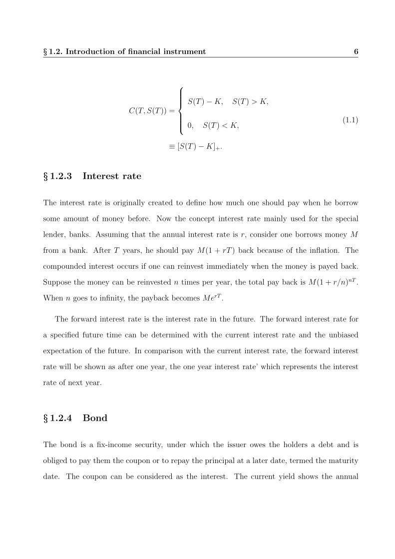
C(T, S(T )) =
S(T )−K, S(T ) > K,
0, S(T ) < K,
≡ [S(T )−K]+.
(1.1)
§ 1.2.3 Interest rate
The interest rate is originally created to define how much one should pay when he borrow
some amount of money before. Now the concept interest rate mainly used for the special
lender, banks. Assuming that the annual interest rate is r, consider one borrows money M
from a bank. After T years, he should pay M(1 + rT ) back because of the inflation. The
compounded interest occurs if one can reinvest immediately when the money is payed back.
Suppose the money can be reinvested n times per year, the total pay back is M(1 + r/n)nT .
When n goes to infinity, the payback becomes MerT .
The forward interest rate is the interest rate in the future. The forward interest rate for
a specified future time can be determined with the current interest rate and the unbiased
expectation of the future. In comparison with the current interest rate, the forward interest
rate will be shown as after one year, the one year interest rate’ which represents the interest
rate of next year.
§ 1.2.4 Bond
The bond is a fix-income security, under which the issuer owes the holders a debt and is
obliged to pay them the coupon or to repay the principal at a later date, termed the maturity
date. The coupon can be considered as the interest. The current yield shows the annual

§ 1.2. Introduction of financial instrument 7
return calculated with the annual coupon payments and the current price of the bond. Let
the current market price be MP and the annual coupon paid be C. The current Yield is CMP
.
The current yield simply shows the return for the total year but it doesn’t include the time
variance. The yield to maturity (YTM) is introduced to show the interest rate including the
future cash flow. The expression of the bond price B is as below
B =C1
(1 + y)1+
C2
(1 + y)2+ ...+
Clast(1 + y)n
, (1.2)
where
Cn is the nth coupon payment,
B is the bond price,
y is the yield to maturity,
Clast is equal to the principal P + CN and
N is the total number of payment.
§ 1.2.5 One type of swaption: bond option
Bond option is a typical swaption that gives the holder the right to buy a bond at the maturity
date. Because both option and bond are including the future time, Bond option is invested
highly depending on the personal prospection of the future market and since the Black-Sholes
model assumes constant volatility [6], which cannot describe the bond option, the Black-Sholes
model cannot easily be used in the bond option.

§ 1.3. Introduction of financial models 8
§ 1.3 Introduction of financial models
§ 1.3.1 Lagrangian model based on supply and demand
In microeconomics, the “supply and demand” is the basic model of price determination for
commodities. It describes the market that in a competitive market, the price of any commodity
will keep changing until it reaches to a point that the quantity demanded equals the quantity
supplied.
Figure 1.2: Supply and Demand in economics
Figure copies from http://www.investopedia.com/university/economics/economics3.asp
The point (P ∗, Q∗) in figure 1.2 is the equilibrium point for one commodity. In physics,
the potential is defined based on supply and demand. The equilibrium point is the deepest
point of the potential V as showed in figure 1.3.
The potential V is designed as below

§ 1.3. Introduction of financial models 9
Figure 1.3: Supply and Demand as potential
V [p] = D[p] + S[p]
= m
[N∑i=1
dipaii
+N∑i=1
sipbii
]; di, si > 0 ; a, b > 0, (1.3)
where di, si, ai, bi are independent constants for each commodity. The Lagrangian is combined
with the potential term and kinetic term. The dynamics of the market are described by the
kinetic term of the Lagrangian. With the numerical analyse, the total Lagrangian is optimised
as the following
L(t) =1
2
N∑i,j=1
[Lij
∂2xi∂t2
∂2xj∂t2
+ Lij∂xi∂t
∂xj∂t
]+
N∑i=1
dipaii
+N∑i=1
sipbii (1.4)
The quantities Lij, Lij, di, si, ai, bi are all real and independent parameters. Matrix Lij is
symmetric and positive definite. Because prices (and quantities) are always positive and
hence represented by exponential variables as pi = pi0exi . The Lagrangian is given by

§ 1.3. Introduction of financial models 10
L(t) =1
2
N∑i,j=1
[Lij
∂2xi∂t2
∂2xj∂t2
+ Lij∂xi∂t
∂xj∂t
]+
N∑i=1
dip0i
e−aixi +N∑i=1
sip0iebixi (1.5)
The Lagrangian given in Eq. (1.5) is nonlinear.
§ 1.3.2 Black-Scholes model for option pricing
In 1973, Fisher Black, Myron Scholes, and Robert Merton gives a mathematical model for a
European option price [6], which is well known as the Black-Sholes model. This model is now
widely used in options market.
The assumptions of the Black-Scholes model are shown as the following:
• No arbitrage opportunity in the market (efficient market)
• People can borrow or lend money at a risk-free rate
• Volatility of the underlying is known and constant
• No transaction fees or dividends during the life of the option
• The log security (return of the security) follows a normal distribution
Let t be the calendar time. The underlying asset price S(t) yields
dS(t)
dt= αS(t) + σS(t)R(t), (1.6)
where α is the drift and σ is the volatility of underlying. The white noise R(t) satisfies
E[R(t)] = 0; E[R(t)R(t′)] = δ(t− t′). (1.7)
§ 1.3. Introduction of financial models 11
Baaquie [7] gave the derivation of Black-Scholes model using path integrals. Let x be lnS.
The Lagrangian and action are simply as below
LBS = −1
2R(t)2, (1.8)
SBS = − 1
2σ2
∫ τ
0
(dx
dt+ α
)2
. (1.9)
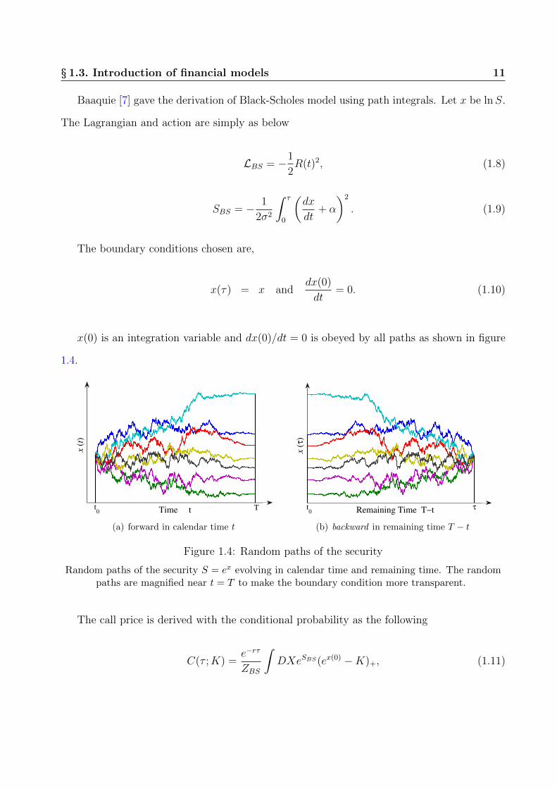
The boundary conditions chosen are,
x(τ) = x anddx(0)
dt= 0. (1.10)
x(0) is an integration variable and dx(0)/dt = 0 is obeyed by all paths as shown in figure
1.4.
Time t
x (
t)
t0
T
(a) forward in calendar time t
Remaining Time T−t
x (
τ)
t0
τ
(b) backward in remaining time T − t
Figure 1.4: Random paths of the security
Random paths of the security S = ex evolving in calendar time and remaining time. The randompaths are magnified near t = T to make the boundary condition more transparent.
The call price is derived with the conditional probability as the following
C(τ ;K) =e−rτ
ZBS
∫DXeSBS(ex(0) −K)+, (1.11)

§ 1.3. Introduction of financial models 12
where
ZBS =∞∏n=0
N∏i=1
∫ ∞−∞
dxnieSBS . (1.12)
From Eq. (1.11), Black-Scholes formula can be derived with the boundary condition as in
Eq. (1.10) and is shown as below
C = SN(d+)− e−rτKN(d−),
d± =ln(S/K) +
(r ± σ2
2
)τ
σ√τ
,
(1.13)
where K is the strike price of the option, σ is the volatility, r is the spot interest rate, and
σ√τ is the standard deviation of x. N(x) is the cumulative distribution given by
N(x) =1√2π
∫ x
−∞e−
12z2dz. (1.14)
The volatility can be calculated by historical data. Since the Black-Sholes model is recog-
nized by financial market, the market quotes the price of option in implied volatility.
§ 1.3.3 HJM Model for forward interest rate
The most widely used model in bond and interest rate field nowadays is Health-Jarraw-
Morton(HJM) model [8]. The forward interest rate f(t, x), is the prediction of interest rate
fixed by future time x > t at time t. The bond market is determined by f(t, x). Let R(t) be
Gaussian white noise and the expectation and correlation of R(t) is given by
E[R(t)] = 0 ; E[R(t)R(t′)] = δ(t− t′).

§ 1.3. Introduction of financial models 13
The HJM model is a linear model
∂f(t, x)
∂t= α(t, x) + σ(t, x)R(t). (1.15)
where α(t, x) is the drift and σ(t, x) is the volatility of data. A single white noise R(t) is
used to describe the forward interest rates but it cannot fully cover the evolution of forward
rate correlation. It is proper to replace the one-dimension white noise by a two-dimension
quantum field A(t, x).
The derivation of the quantum HJM model [1] is shown as below
∂f
∂t(t, x) = α(t, x) + σ(t, x)A(t, x), (1.16)
f(t∗, x) = f(t0, x) +
∫ t∗
t0
dtα(t, x) +
∫ t∗
t0
dtσ(t, x)A(t, x), (1.17)
where the drift can be calculated by martingale as the following
α∗(t, x) = σ(t, x)
∫ x
t∗
dx′D(x, x′; t)σ(t, x′). (1.18)

Chapter 2
Multiple Commodities in Statistical
Microeconomics: Model and Market
§ 2.1 Introduction
The theory of prices proposed in [9] is based on the concept of the action functional; the
subsequent publication [4] provides strong empirical evidence in support of this formulation for
the case of single commodities. The present paper extends the analysis to multi-commodities
by modifying the single commodity model in a parsimonious manner.
The theory of commodity prices [10] is one of the bedrocks of microeconomics and usually
starts with the concept of the utility function of a typical consumer [11, 12] . A maximization
of the utility function with a budget constraint yields the demand for the commodities as a
function of price. The supply function is obtained by maximizing the profit for the producers
and the market prices of commodities in conventional microeconomics are fixed by equating
supply with the demand[11, 12].
In contrast to conventional microeconomics, in statistical microeconomics [9] the prices
of all commodities are taken to be intrinsically random – and the probability distribution
function of prices is fixed by the exponential of the so called action functional. The action
14

§ 2.1. Introduction 15
functional in turn is the sum of two parts, a ‘kinetic’ term that determines the dynamical
evolution of commodity prices and a microeconomic potential that is the sum of the supply
and demand functions. The action functional contains all the information of the market and
determines the distribution of market prices as well as the change in market prices as the
prices evolve in time [13, 14, 15].
The primary focus in the statistical microeconomic formulation is to describe the unequal
time correlation functions of market prices. The auto- and cross-correlation [16, 17] functions
for multiple commodities is modeled using the action functional and the Feynman path inte-
gral. The action functional is calibrated by matching the prediction of the model’s correlation
functions with the observed market and provides a stringent test of the accuracy of the model.
The microeconomic potential for commodity with price p is given by V [p] and has been
introduced in [9]; the potential has its minimum value at its extrema p, given by
∂V [p]/∂p = 0.
The price p is taken to be the average commodity price.
What happens when the price p is not equal to the average price p, that is, p 6= p? The
microeconomic potential V [p] in this case causes the prices to ‘move’, that is, to change and
tend towards p. Clearly, the more abrupt the change, the more unlikely it is; the change of
price should, for normal market conditions, be gradual and relatively ‘smooth’. To achieve this
smooth movement of the prices in general, a ‘kinetic term’ T [p(t)] is introduced. Although
the concept of the kinetic term is taken from physics, it finds a natural expression in the
evolution of the prices of commodities: the specific form of the kinetic term is determined by
the study of market data [9]. The kinetic term in the action functional is seen to be strongly
supported by market data, and as of now has no clear theoretical explanation. One can only
speculate that demand and supply are determined by consumers and producers, respectively

§ 2.2. The microeconomic action functional 16
and that the kinetic term reflects the process of circulation, distribution and exchange – as
well as the degree of market liquidity – that is necessary for the products to make a transition
from the producer to the final consumer in the market.
One rather unexpected result is that the kinetic term in the action functional has a domi-
nant role in the evolution of commodity prices; due to the high time derivative of prices in the
kinetic term, the short term evolution of commodity prices is completely dominated by the
kinetic term, with the microeconomic potential, containing the supply and demand functions,
come into play for the long term evolution.
§ 2.2 The microeconomic action functional
Consider N commodities, with market prices given by pI ; I = 1, .., N . Prices are always pos-
itive and can be represented by exponential variables as pI = p0exI ; the normalized logarithm
of prices, denoted by xI , is defined as follow
pI = p0IexI ; xI(t) = ln(pI(t)/p0I) ; I = 1, .., N.
The demand function and the supply function are modeled to be [9]
D[p] =N∑i=1
dip0ie−aixi ; S[p] =
N∑i=1
sip0iebixi ; di, si > 0 ; a, b > 0. (2.1)
The coefficients di, si, according to [9], are determined by macroeconomic factors such as
interest rates, unemployment, inflation and so on.
For the purpose of modeling, prices in statistical microeconomics are expressed in terms
of variables that are measured from the average value and normalized by the volatility of the

§ 2.2. The microeconomic action functional 17
stock.
yi(t) =xi(t)− xi
σi; i = 1, .., N. (2.2)
xI and σI are the average value of yI . The volatility of xI(t) for the time period being
considered and are given by
xi = E[xi] ; σ2i = E[
(xi − xi
)2].
The normalized variables yi are all of O(1) and hence one can model and compare commodities
with vastly different volatilities and prices. In the statistical microeconomic approach, the
microeconomic potential is the fundamental quantity that combines supply and demand by
considering their sum [9]. The supply and demand yield the microeconomic potential given
by
V =N∑i=1
[dip0ie
aixie−aiσiyi + sip0ie−bixiebiσiyi
]≡
N∑i=1
[die−aiyi + sie
biyi], (2.3)
where
di = dip0ieaixi ; si = sip0ie
−bixi ; ai = aiσi ; bi = biσi.
For the case of multiple commodities, the microeconomic potential for the N -commodities
is further generalized by including a term that depends on the product of the prices of com-
modities – and which cannot be placed either in the demand or in the supply component of
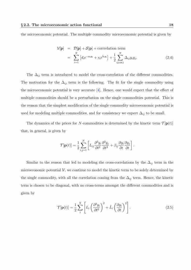
§ 2.2. The microeconomic action functional 18
the microeconomic potential. The multiple commodity microeconomic potential is given by
V [p] = D[p] + S[p] + corrrelation term
=N∑i=1
[die−aiyi + sie
biyi]
+1
2
N∑ij;i 6=j
∆ijyiyj. (2.4)
The ∆ij term is introduced to model the cross-correlation of the different commodities.
The motivation for the ∆ij term is the following. The fit for the single commodity using
the microeconomic potential is very accurate [4]. Hence, one would expect that the effect of
multiple commodities should be a perturbation on the single commodities potential. This is
the reason that the simplest modification of the single commodity microeconomic potential is
used for modeling multiple commodities, and for consistency we expect ∆ij to be small.
The dynamics of the prices for N -commodities is determined by the kinetic term T [p(t)]
that, in general, is given by
T [p(t)] =1
2
N∑i,j=1
[Lij
∂2yi∂t2
∂2yj∂t2
+ βij∂yi∂t
∂yj∂t
].
Similar to the reason that led to modeling the cross-correlations by the ∆ij term in the
microeconomic potential V , we continue to model the kinetic term to be solely determined by
the single commodity, with all the correlation coming from the ∆ij term. Hence, the kinetic
term is chosen to be diagonal, with no cross-terms amongst the different commodities and is
given by
T [p(t)] =1
2
N∑i
[Li
(∂2yi∂t2
)2
+ Li
(∂yi∂t
)2]. (2.5)

§ 2.2. The microeconomic action functional 19
The Lagrangian is given by the sum of the kinetic and potential factors and yields [9]
L(t) = T [p(t)] + V [p(t)].
The Lagrangian, from Eqs. (2.4) and (2.5), is the following
L(t) =1
2
N∑i
[Li
(∂2yi∂t2
)2
+ Li
(∂yi∂t
)2]
+N∑i=1
[die−aiyi + sie
biyi]− 1
2
N∑ij;i 6=j
∆ijyiyj. (2.6)
The Lagrangian given in Eq. (2.6) is nonlinear.
The action functional determines the dynamics (time evolution) of market prices and is
given by
A[p] =
∫ +∞
−∞dtL(t) =
∫ +∞
−∞dt(T [p(t)] + V [p(t)]
).
All prices of commodities are considered to be stochastic variables and the action functional
is assumed to determine the probability distribution, which is given by
Probability distribution for a specific time evolution ∝ e−A[y]
All correlation functions of the prices are given by the Feynman path integral [9, 3]
D123...n(t1, t2, ...tn) = E[y1(t1)y2(t2) · · · yn(tn)] =1
Z
∫Dye−A[y]y1(t1)y2(t2) · · · yn(tn)
with
Z =
∫Dye−A[y].

§ 2.3. Correlation Function 20
§ 2.3 Correlation Function
We study the leading terms in the Lagrangian by doing a Taylor expansion of the potential
term V about its minima, which will turn out to coincide with an expansion of V in a power
series in yi.
The minima xi is defined by
∂V(x)
∂xi= 0.
Hence from Eq. (2.4)
∂V(x)
∂xi= −aidip0ie
aixi + bisip0iebixi −
∑j,i6=j
∆ij(xj − xjσj
) = 0. (2.7)
In our model, we assume that the equilibrium price of the commodities x is given by its
average value x and yields
xi = xi. (2.8)
Hence, from Eq. (2.7)
− aidieaixi + bisiebixi = 0. (2.9)
Note that Eq. (2.9) is independent of p0i and hence p0i does not enter the calibration of the
model’s parameters. Eq. (2.9) yields
exi =
(aidi
bisi
)(1/(ai+bi))
. (2.10)
Eqs. (2.3), (2.8) and (2.10) yield
aidi = bisi. (2.11)

§ 2.3. Correlation Function 21
§ 2.3.1 Expansion of Potential
From the definition of yi given in Eq. (2.2), the minima of the action is about yi = 0. Hence,
expanding the Lagrangian about yi = 0 yields
L =∑i
(1
2Liyi
2 +1
2Liyi
2 +γi2y2i +
αi3!y3i +
βi4!y4i + · · · )− 1
2
∑ij,i6=j
∆ijyiyj.
Define the Lagrangian in terms of the quadratic and nonlinear terms as follow
L = L2 + L3 + L4 +O(y5).
L2(x) are the quadratic terms in the expansion of the Lagrangian given above and L3(x),L4(x)
are the cubic and quartic terms.
The quadratic Lagrangian is given by
L2 = L0 + Lc,
L0 =1
2
∑i
[Liyi
2 + Liyi2 + γiy
2i
]; Lc = −1
2
∑ij;i 6=j
∆ijyiyj,
and the nonlinear terms are
L3 =αi3!y3i ; L4 =
βi4!y4i .
The action is given by the following
A = A0 +Ac +AI =
∫dtL;
A0 =
∫dtL0 ; Ac =
∫dtLc
AI =
∫dt(L3 + L4).

§ 2.3. Correlation Function 22
From above we have
γi =1
2(dia
2i + sib
2i ), (2.12)
αi = (−a3i di + b3
i si) = (bi − ai)γi, (2.13)
βi = (a4i di + b4
i si) = (a2i − aibi + b2
i )γi. (2.14)
The linear term in yi is zero due to Eq. (2.11). We will determine the values of α, β, γ, y from
market data; the potential parameter of ai, bi, si, di are then given by the following
ai =±√
4βiγi − 3α2i − αi
2γi; bi = ai +
αiγi
;
si =γi
bi(ai + bi); di =
γiai(ai + bi)
.
The positive branch for ai is used since ai > 0.
§ 2.3.2 Auto-correlation
The correlation function for the A0 is given by the Gaussian propagator
D(0)(t− t′) =1
Z
∫Dye−A0[y]yI(t)yJ(t′).
and the auto-correlation function is given by
D(0)II (t− t′) ≡ D
(0)I (t− t′) =
1
Z
∫Dye−A0[y]yI(t)yI(t
′) +O(∆2).

§ 2.3. Correlation Function 23
Using a Fourier transform to evaluate the propagator for the prices, and dropping the
subscript I, yields
D(0)(t− t′) ≡∫ ∞−∞
dk
2π
eik(t−t′)
Lk4 + Lk2 + γ=
e−√a−|t−t′|√a−
− e−√a+|t−t′|√a+
2L(a+ − a−);
a± =L
2L± | L
2L|
√1− 4Lγ
L2.
Case I: Real branch. 4Lγ < L2 and a± is real; let
ω = (γ
L)14 , a± =
√γ
Le±2ϑ, e±2ϑ =
√L2
4Lγ+
√L2
4Lγ− 1.
Hence D(0)(t− t′) is given by
D(0)(t− t′) =ωe−ω|t−t
′| cosh(ϑ)
2γ sinh(2ϑ)sinh[ϑ+ ω|t− t′| sinh(ϑ)].
Case II: Complex branch. 4Lγ > L2 and a± are complex; let
ω = (γ
L)14 , a± =
√γ
Le±i2φ, cos(2φ) =
√L2
4Lγ, sin(2φ) =
√1− L2
4γL. (2.15)
We hence obtain the complex branch propagator
D(0)(t− t′) =ωe−ω|t−t
′| cos(φ)
2γ sin(2φ)sin[φ+ ω|t− t′| sin(φ)].
Define the normalization constant
N =ω
2γ sin 2φ.

§ 2.3. Correlation Function 24
and yields the complex branch propagator
D(0)(t− t′) = N e−ω|t−t′| cos(φ) sinφ+ ω|t− t′| sin(φ). (2.16)
The auto-correlation function of commodities will be seen to follow the behavior given by the
complex branch. The real branch cannot describe the data from market.
§ 2.3.3 Cross-correlation
The cross-correlation function is given by I 6= J. The model yields
E[yI(0)yJ(τ)] = DIJ(t) =1
Z
∫Dye−(A0+Ac)yI(0)yJ(τ)
=1
Z
∫Dye−A0[y]yI(0)yJ(τ)
[1 +
1
2
∑ij;i 6=j
∆ij
∫dtyi(t)yj(t) +O(∆2)
].
The first term is zero and hence
DIJ(τ) ' D(0)IJ (t), (2.17)
where
D(0)IJ (t) ≡
∫ ∞−∞
D(0)I (t)D
(0)J (t− τ)dt.
From Appendix Eq. (2.28):
D(0)IJ (t) =
C
LILJ
( 1
αe−|t|α cosφ[
1
R(h1/R) cos φ− (h2/R) sin φ − 1
T(h3/T ) cos φ− (h4/T ) sin φ]
+1
βe−|t|βcosθ[
1
P(h5/P ) cos θ − (h6/P ) sin θ − 1
Q(h7/Q) cos θ − (h8/Q) sin θ]
),
(2.18)
§ 2.3. Correlation Function 25
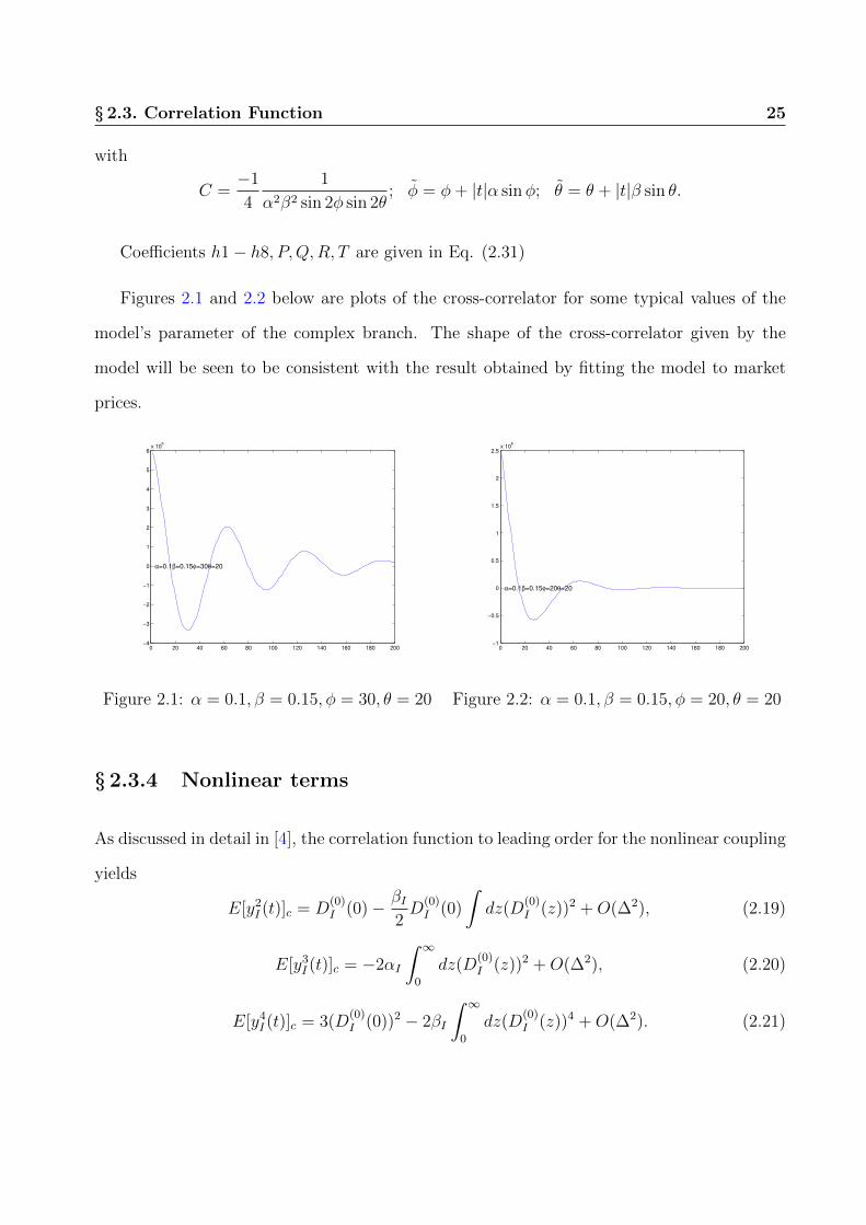
with
C =−1
4
1
α2β2 sin 2φ sin 2θ; φ = φ+ |t|α sinφ; θ = θ + |t|β sin θ.
Coefficients h1− h8, P,Q,R, T are given in Eq. (2.31)
Figures 2.1 and 2.2 below are plots of the cross-correlator for some typical values of the
model’s parameter of the complex branch. The shape of the cross-correlator given by the
model will be seen to be consistent with the result obtained by fitting the model to market
prices.
0 20 40 60 80 100 120 140 160 180 200−4
−3
−2
−1
0
1
2
3
4
5
6x 10
6
α=0.1β=0.15φ=30θ=20
Figure 2.1: α = 0.1, β = 0.15, φ = 30, θ = 20
0 20 40 60 80 100 120 140 160 180 200−1
−0.5
0
0.5
1
1.5
2
2.5x 10
6
α=0.1β=0.15φ=20θ=20
Figure 2.2: α = 0.1, β = 0.15, φ = 20, θ = 20
§ 2.3.4 Nonlinear terms
As discussed in detail in [4], the correlation function to leading order for the nonlinear coupling
yields
E[y2I (t)]c = D
(0)I (0)− βI
2D
(0)I (0)
∫dz(D
(0)I (z))2 +O(∆2), (2.19)
E[y3I (t)]c = −2αI
∫ ∞0
dz(D(0)I (z))2 +O(∆2), (2.20)
E[y4I (t)]c = 3(D
(0)I (0))2 − 2βI
∫ ∞0
dz(D(0)I (z))4 +O(∆2). (2.21)

§ 2.4. Market data and model 26
Some integrations that are useful to solve the potential prameters a, b, s, d are the following
[3] ∫ ∞0
D(0)(τ)dτ = N sin 2φ
ω,
∫ ∞0
(D(0)(τ))2dτ = N 2 secφ− cos 3φ
4ω,
∫ ∞0
(D(0)(τ))3dτ = N 3 2 sin3 φ(11 cosφ+ 2 cos 3φ)
4ω,
∫ ∞0
(D(0)(τ))4dτ = N 4 sinφ3(50 cos 2φ+ 6 cos 4φ+ 47) tanφ
16ω(3 cos 2φ+ 5).
Using four equations 2.11, 2.19, 2.20 and 2.21, potential parameters ai, bi, si, di can be ob-
tained.
§ 2.4 Market data and model
The empirical correlator is denoted by the notation of GIJ(t) and is defined by the expectation
value of the market prices. For a time series data set with time interval of ε, the prices are
given by yI(t) = yI(n), where t = nε and we have τ = kε; for N data points, the correlator is
given by the moving average
GIJ(τ) = GIJ(k) = E[yI(0)yJ(k)]c
∣∣∣market
=1
N
N−k∑n=0
yI(n)yJ(n+ k).
The numerical evaluation of the correlators is obtained by taking the moving average over the
data set. The model always yields a correlator that is a symmetric function of IJ , which is
not necessarily the case for the market correlator [9]. To equate the market correlator with
the model, it is made symmetrically, namely
GIJ(τ) = GJI(τ).

§ 2.4. Market data and model 27
and in terms of the underlying data we have
GIJ(τ) =1
2[
1
N
N−k∑n=0
yI(n)yJ(n+ k) +1
N
N−k∑n=0
yJ(n)yI(n+ k)].
The parameter of time for the market and model are not the same. The reason being that
time for traders is determined by the liquidity of the market and rate of transactions [7]. To
reflect this feature of the market, define market time z(τ) by
τ → z(τ).
The empirical correlator G(τ) is given by the exact model correlator D(τ) by the relation
GIJ(t) = DIJ(z(t)). (2.22)
For single commodity fit
D(0)II (z(t)) = N e−ωIz(t) cos(φI) sinφI + ωIz(t) sin(φI).
For cross-correlation DIJ , we use Eq. (2.18) to fit the market cross-correlator.
According to Ref. [4], for single commodity fit, using GII(t) ≡ GI(t), we have
GI(t) = D(0)I (z(t))− βI
2D
(0)I (0)
∫dτD
(0)I (z(t)− τ)D
(0)I (τ) +O(∆2). (2.23)
Let∫dτ(D
(0)I (τ))2 = CI . When τ equals to zero,
GI(0) ' D(0)I (0)− βI
2D
(0)I (0)CI = D
(0)I (0)(1− βI
2CI). (2.24)

§ 2.5. Fitting with Market Data 28
For the auto-correlation GII , note that the empirical definition of x and σ implies that
GI(0) = 1.
Hence
1 = GI(0) = D(0)I (0)− βI
2D
(0)I (0)CI ⇒ D
(0)I (0) =
1
1− βI2CI. (2.25)
Eq. (2.25) is consistent with Eq. (2.24). Substituting D(0)I (0) into GI(t), for t > 0 – using
Eq. (2.16) for the numerator and denominator – we obtain1
GI(t) =D
(0)I (z(t))
D(0)I (0)
=1
sinφe−ωz(t) cos(φ) sinφ+ ωz(t) sin(φ). (2.26)
We use D(0)I (z(t))/D
(0)I (0) to fit GI(t) in the single commodity case. Hence, once we have
obtained φI , ωI all the parameters of the complex branch of the model can be determined.
§ 2.5 Fitting with Market Data
As a rule, the correlators evaluated from the data are denoted by GIJ and the result obtained
by fitting the model are denoted by DIJ . The numbering for the indices I, J for the various
commodities is the one given in Table 2.1.
We analyze 18 commodities daily data drawn from four major groups of energy, metal,
food, grain, from 2014/01/01 to 2015/02/03 download from
Investing.com/commodities/real-time-futures.2 Since the correlators are symmetric, there are
1The approximation makes the result consistent with the value of GI(0) = 1.2Real-time streaming quotes for the top commodities futures CFDs. The quotes are available for a variety
of futures such as Gold, Crude Oil, Silver, Copper and many more Metals, Energies and Softs futures. Thelatest price as well as the daily high, low and the change for each future. The ”Base” price is the last close of

§ 2.5. Fitting with Market Data 29
153 correlators in total, with 18 auto-correlation functions and 153 cross-correlation functions.
Table 2.1: Number and Type of Commodity
Number commodity Type Number commodity Type
1 Crudeoil Energy 10 Cocoa Food
2 Heatingoil 11 Soybeansoil
3 Brentoil 12 Orangejuice
4 Natural gas 13 Livecattle
5 Copper Metal 14 Wheat Grain
6 Gold 15 Corn
7 Silver 16 Soybean
8 Platinum 17 Roughrice
9 Palladium 18 Cotton Misc
All the auto-correlation functions can be fit to a high degree of accuracy and confirms the
results found in [4] for single commodities.
The model can fit the majority of the cross-correlators Gij(i 6= j) which are generically
similar to the shape that the model generates from Eq. (2.18) and shown in Figures 2.1 and
2.2. Of the 153 cross-correlators, 110 are of the shape that the model can fit quite well. The
rest of the cross-correlators Gij have features that the model cannot fit; in particular, if the
each future contract (as of 16:30 ET). The change is calculated from the ”Base” price.

§ 2.5. Fitting with Market Data 30
cross-correlator has a maximum value at a time lag that is non-zero, then there are no choice
of parameters for Gij that can fit the cross-correlator.
The fitting is based on Eqs. (2.17) and (2.22)
GIJ(τ) = DIJ(z(τ)) ; I 6= J.
To leading order we approximate DIJ(t) by the Gaussian approximation D(0)IJ (t) given in
Appendix § 4.11.1 and obtain
GIJ(τ) ' D(0)IJ (z(τ)) = ∆IJ
∫ ∞−∞
dtD(0)I (t)D
(0)J (t− z(τ)) ; I 6= J.
Hence, the cross-correlation coupling ∆IJ is given by
GIJ(0) = ∆IJ
∫ ∞−∞
dtD(0)I (t)D
(0)J (t) ; I 6= J. (2.27)
The empirical cross-correlation of 18 commodities has been studied. Anticipating results
derived later on in the paper, the parameters ∆IJ are given in Figure 2.3 for all the cross-
correlators.

§ 2.5. Fitting with Market Data 31
5
10
15
0
5
10
15
20
−0.04
−0.02
0
0.02
0.04
0.06
0.08
0.1
0.12
Figure 2.3: Matrix of ∆ij for 18 commodities. Note that for all pairs, |∆IJ | < 0.08 but onecase.
The fitting of market correlator to the model is done in the following.
• Simultaneously fit all the auto-correlation functions DII(z(t)) = DI(z(t)) with the G(t),
as in Eq. (2.26), and evaluate the parameters ω, φ, η, λ. The value of η, λ does not enter
into the calibration of the other parameters.
• Using the values of ω, φ, as in Eq. (2.26), and the nonlinear terms given Eq.(2.19),
(2.20), (2.21), we evaluate L, L, γ, α and β.
• Use the parameters L, L, γ, α and β as in Eq. (2.11), (2.12), (2.13), (2.14) and find [a,
b, s, d].
• Evaluate the cross-correlation function DIJ ; I 6= J and determine ∆IJ .
• The correlators are fitted for a maximum time of lag τ = 200 days.
Note the remarkable fact, that ignoring one cross-correlator, the value of all the ∆IJ ’s is
such that |∆IJ | < 0.08. The fact |∆IJ | < 0.08 provides strong evidence of the correctness

§ 2.5. Fitting with Market Data 32
of our approach of considering the multi-commodities model as a perturbation of the single
commodities, which requires |∆IJ | << 1.
Note in extending the statistical model from single to N commodities, N(N − 1)/2 new
parameters ∆IJ are introduced, which in turn are fixed by only a single value of the cross-
correlators GIJ(0), as given in Eq. (2.27).
For our model, the entire dependence of GIJ(τ) for time lag τ > 0 is determined by the
auto-correlation functions D(0)I (z(τ)) and its convolution with itself – as given in Eq. (2.17).
The fact that the model can accurately describe all the auto- and cross-correlators, up to
N = 4 commodities, provides evidence for the correctness of the model. We will discuss
later how the model can be extended to accurately describe a collection of commodities with
arbitrary N .
Calibration for cocoa
1. Use cross-correlation Eq. (2.18) and auto-correlation Eq. (2.16) to fit each data to find ω
φ, λ, and η.
2. Substitute ω, φ, λ, and η into Eq. (2.19), (2.20), (2.21) and (2.15) to get γ, L, L, αI , βI
3. Using the value of all parameters obtained above as in Eq. (2.11), (2.12), (2.13), (2.14),
we can determine the indices [a, b, s, d] [4] of supply and demand function. The result obtained
in Table § 2.6.2 for cocoa from the fitting of the Crude oil, Platinum and Cocoa group is used

§ 2.6. Fits for GII , GIJ 33
below to illustrate the fitting procedure.
ω = 0.1535, φ = 1.2229, λ = 0.700, η = 0.54
⇒ γ = 0.113, L = 203.37, L = −7.35, α = 0.0199, β = 0.0747
⇒∫ ∞
0
dτG(τ) = 4.4413;
∫ ∞0
dτG2(τ) = 6.9973;∫ ∞0
dτG3(τ) = 4.5490;
∫ ∞0
dτG4(τ) = 4.2909
⇒ a = 0.72, b = 0.90, s = 0.094, d = 0.075
§ 2.6 Fits for GII , GIJ
All the fits of the model with data are carried out using the equations for the correlation
functions given in Eqs. (2.16) and (2.18). All auto-correlators are normalized such that
GII(0) = DII(0) = 1. However, for displaying the results clearly, the entire auto-correlator
is rescaled – such that sometimes we scale to GII(0) > 1 or GII(0) < 1 – so that the results
for the different commodities do not overlap and can be viewed clearly. Similarly, the cross-
correlators are also scaled and for four or more commodities are also shifted to avoid an overlap
of the graphs.
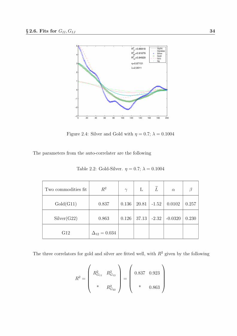
§ 2.6.1 Two commodities
Any two commodities, from different types as given in Table 2.1, can be fit to a high degree
of accuracy. The fit is even better if the two commodities belong to the same type. Figure
2.4 shows the fit for Gold and Silver.
§ 2.6. Fits for GII , GIJ 34
0 20 40 60 80 100 120 140 160 180 200−3
−2
−1
0
1
2
3
4
5
R2
11=0.86918
R2
22=0.91679
R2
12=0.84929
η=0.87151
λ=2.0011
Gij(fit)
Gij(data)
Silver
Gold
G(ii)
Gjj
Figure 2.4: Silver and Gold with η = 0.7; λ = 0.1004
The parameters from the auto-correlater are the following
Table 2.2: Gold-Silver. η = 0.7; λ = 0.1004
Two commodities fit R2 γ L L α β
Gold(G11) 0.837 0.136 20.81 -1.52 0.0102 0.257
Silver(G22) 0.863 0.126 37.13 -2.32 -0.0320 0.230
G12 ∆12 = 0.034
The three correlators for gold and silver are fitted well, with R2 given by the following
R2 =
R2G11
R2G12
* R2G22
=
0.837 0.923
* 0.863

§ 2.6. Fits for GII , GIJ 35
§ 2.6.2 Three commodities fit
We study commodities from the same group and from different groups as well.
Three commodities in same group
The figures for three commodities in one group are given below.
Crude oil-Heating oil-Brent oil:
0 20 40 60 80 100 120 140 160 180 200−4
−2
0
2
4
6
8
10
Crudoil(G11)
Heatoil(G22)
Brentoil(G33)
D11
D22
D33
0 20 40 60 80 100 120 140 160 180 200−10
0
10
20
30
40
50
D13(fit)
G13(data)
D23(fit)
G23(data)
D12(fit)
G12(data)
(a) (b)
Figure 2.5: Crude oil-Heating oil-Brent oil (a)Autocorrelation and (b)Crosscorrelation withη = 0.7; λ = 0.775
Table 2.3: Crude oil-Heating oil-Brent oil. η = 0.7; λ =
0.775
Three commodities fit R2 γ L L α β
Crude oil(G11) 0.804 0.0539 171.4 -1.434 0.0613 0.0813
Heating oil(G22) 0.797 0.0537 158.6 -1.182 0.0677 0.0688

§ 2.6. Fits for GII , GIJ 36
Brent oil(G33) 0.798 0.0536 167.4 -1.329 0.0638 0.0738
GIJ ∆12 = 0.032 ∆13 = 0.031 ∆23 = 0.032
R2 =
0.804 0.918 0.921
* 0.797 0.923
* * 0.798
Orange juice-Cattle-Soybean:
0 20 40 60 80 100 120 140 160 180 200−4
−2
0
2
4
6
8
10
Orangejuice(G11)
Cattle(G22)
Soybean(G33)
D11
D22
D33
0 20 40 60 80 100 120 140 160 180 200−30
−20
−10
0
10
20
30
40
D13(fit)
G13(data)
D23(fit)
G23(data)
D12(fit)
G12(data)
(a) (b)
Figure 2.6: Orange juice-Cattle-Soybean (a)Autocorrelation and (b)Crosscorrelation with η =0.7;λ = 1.132
Table 2.4: Orangejuice-Cattle-Soybean. η = 0.7;λ =
1.132
Three commodities fit R2 γ L L α β

§ 2.6. Fits for GII , GIJ 37
Orange juice(G11) 0.609 0.0512 116.06 0.0032 -0.0049 0.0057
Cattle(G22) 0.733 0.0477 236.95 -1.48 0.0290 0.0776
Soybean(G33) 0.685 0.0425 225.14 -0.308 -0.0576 0.0595
GIJ ∆12 = −0.030 ∆13 = 0.021 ∆23 = −0.019
R2 =
0.609 0.875 0.727
* 0.733 0.781
* * 0.685

§ 2.6. Fits for GII , GIJ 38
Gold-Silver-Platinum:
0 20 40 60 80 100 120 140 160 180 200−5
0
5
10
Gold(G11)
Silver(G22)
Plati(G33)
D11
D22
D33
0 20 40 60 80 100 120 140 160 180 200−10
0
10
20
30
40
50
D13(fit)
G13(data)
D23(fit)
G23(data)
D12(fit)
G12(data)
(a) (b)
Figure 2.7: Gold-Silver-Platinum (a)Autocorrelation and (b)Crosscorrelation with η = 0.7;λ = 0.344
Table 2.5: Gold-Silver-Platinum. η = 0.7; λ = 0.344
Three commodities fit R2 γ L L α β
Gold(G11) 0.827 0.0908 58.6 -1.863 0.0071 0.179
Silver(G22) 0.803 0.0752 88.1 -4.17 -0.0217 0.159
Platinum(G33) 0.799 0.0726 112.1 -2.26 -0.0320 0.180
GIJ ∆12 = 0.033 ∆13 = 0.031 ∆23 = 0.025

§ 2.6. Fits for GII , GIJ 39
R2 =
0.827 0.931 0.910
* 0.803 0.895
* * 0.799
Three commodities from different groups
Crude oil-Platinum-Cocoa:
0 20 40 60 80 100 120 140 160 180 200−4
−2
0
2
4
6
8
10
Crudoil(G11)
Plati(G22)
Cocoa(G33)
D11
D22
D33
0 20 40 60 80 100 120 140 160 180 200−15
−10
−5
0
5
10
15
20
25
30
35
G13(fit)
G13(data)
G23(fit)
G23(data)
G12(fit)
G12(data)
(a) (b)
Figure 2.8: Crude oil-Platinum-Cocoa (a)Autocorrelation and (b)Crosscorrelation with η =0.70; λ = 0.54.
Table 2.6: Crude oil-Platinum-Cocoa. η = 0.70; λ = 0.54
Three commodities fit R2 γ L L α β
Crude oil(G11) 0.871 0.0560 286.3 -3.54 0.0566 0.0742
Platinum(G22) 0.835 0.0585 305.2 -4.17 -0.0241 0.1346

§ 2.6. Fits for GII , GIJ 40
Cocoa(G33) 0.920 0.113 203.4 -7.35 0.0199 0.0747
GIJ ∆12 = 0.021 ∆13 = 0.045 ∆23 = 0.023
R2 =
0.871 0.612 0.920
* 0.835 0.943
* * 0.920
The R2 of three commodities fit are normally between 0.8-1. Although they are not quite
high, the values are high enough to be convincing.
§ 2.6.3 Four commodities
When we consider taking more commodities into the fit, such as 4 and 6 commodities, the fit
is not so good.

§ 2.6. Fits for GII , GIJ 41
0 20 40 60 80 100 120 140 160 180 200−30
−25
−20
−15
−10
−5
0
Silver(G11)
Gold(G22)
Crudeoil(G33)
Gas(G44)
D11
D22
D(33)
D(44)
0 20 40 60 80 100 120 140 160 180 200−20
0
20
40
60
80
100
D14(fit)
G14(data)
D24(fit)
G24(data)
D34(fit)
G34(data)
D13(fit)
G13(data)
D23(fit)
G23(data)
D12(fit)
G12(data)
(a) (b)
Figure 2.9: Gold-Silver-Crude oil-Natural gas (a)Autocorrelation and (b)Crosscorrelation withη = 0.70; λ = 0.260.
Four commodities fit R2 γ L L α β
Gold(G11) 0.834 0.0973 54.9 -2.051 0.0074 0.186
Silver(G22) 0.827 0.0835 105.2 -2.940 -0.0220 0.159
Crude oil(G33) 0.749 0.0769 35.3 -0.041 0.0962 0.128
Natural gas(G44) 0.377 0.0667 81.8 -0.921 0.0850 0.015
Table 2.7: Gold-Silver-Crude oil-Natural gas. η = 0.70;
λ = 0.260.

§ 2.6. Fits for GII , GIJ 42
R2 =
0.834 0.885 0.507 0.074
* 0.827 0.725 0.435
* * 0.749 0.809
* * * 0.377
As can can be seen from Table 2.7, the R2 of four commodities fit goes down to 0.7-0.9 and
for some is in the range 0.4-0.7. So the fit seems to fail to give a good result when we consider
four commodities.
§ 2.6.4 Six commodities
0 20 40 60 80 100 120 140 160 180 200−30
−20
−10
0
10
20
30
40
Gold(G11)
D(11)
Silver(G22)
D(22)
Crudoil(G33)
D(33)
Gas(G44)
D(44)
Soyboil(G55)
D(55)
Cattle(G66)
D(66)
0 20 40 60 80 100 120 140 160 180 200−40
−20
0
20
40
60
80
D12fitG12dataD13fitG13dataD14fitG14dataD15fitG15dataD16fitG16dataD23fitG23dataD24fitG24dataD25fitG25dataD26fitG26dataD34fitG34dataD35fitG35dataD36fitG36data’D45fitG45data’D46fitG46data’D56fitG56data
(a) (b)
Figure 2.10: Gold-Silver-Crude oil-Natural gas-Soybean oil-Cattle (a)Autocorrelation and(b)Crosscorrelation with η = 0.70; λ = 0.699.
Table 2.8: Gold-Silver-Crude oil-Natural gas-Soybean
oil-Cattle. η = 0.70; λ = 0.699.

§ 2.6. Fits for GII , GIJ 43
Six commodities fit R2 γ L L α β
Gold(G11) 0.825 0.0794 92.02 -2.259 0.0062 0.155
Silver(G22) 0.566 0.0637 15.36 1.948 -0.0269 0.203
Crude oil(G44) 0.512 0.0863 6.09 1.448 0.1351 0.184
Natural gas(G44) 0.443 0.0520 185.1 -1.394 0.0654 0.0118
Soybean oil(G55) 0.447 0.116 2.51 1.078 -0.1718 0.268
Cattle(G66) 0.447 0.198 2.270 1.050 0.0987 0.2717
R2 =
0.825 0.935 0.281 0.011 0.265 0.727
* 0.566 0.573 0.483 0.291 0.701
* * 0.512 0.789 0 0.033
* * * 0.443 0 0.064
* * * * 0.447 0
* * * * * 0.447
The R2 of six commodities fit can not be considered to be a good fit.

§ 2.7. Comparison of single and multiple commodities fit 44
§ 2.7 Comparison of single and multiple commodities fit
There are two different procedures for doing the fit for a given commodity: by using the
single commodity data and the other by doing a fit for multiple commodities. The purpose
of this exercise is to ascertain how much do the prices of other commodities affect a given
commodity’s prices. We also need to verify that the multi-commodity prices are in fact a
perturbation to the single commodity fit of the prices of a given commodity.
• A given commodity is calibrated using only the data for the given commodity. This is
denoted by S-commodity in Table 2.9.
• The same commodity is calibrated by doing a fit for the commodities for all the groups
and maximizing the goodness of fit for this collection of commodities, including choosing
the best value for the cross-correlation parameters ∆ij’s. This fit is denoted by M-
commodity in Table 2.9.
• In Table 2.9, Group A is a simultaneous fit for three commodities, with two commodities
from metal and the other from energy. In Group B of Table 2.9, three commodities
from different groups, namely one from energy, one from metal and one from food are
calibrated using our model.
• The single commodity fit has an R2 above 0.94 whereas when the multiple commodity
fit is done, R2 is still good but now about 0.80.
Most of the parameters between single commodity fit and multiple commodities fit are
similar. The potential constants a, b, s, d given in Eq.(2.1), as well as the market time param-
eters η, λ changes by about 10% in going from the single to the three commodities fit. This
verifies our intuition that the price of a single commodity is mostly, up to 90%, determined
by its own dynamics, with the other commodities being a perturbation on its prices. Hence,

§ 2.7. Comparison of single and multiple commodities fit 45
while it is true that single commodity fit is more accurate than the multiple fit, the multiple
commodity fit contains the influence from other commodities and hence reflects the market
more accurately.
Table 2.9: Comparison of Single-Commodity fit(S-) with
Multiple-Commodities fit(M-). Group 1 is Gold-Silver-
Crude oil (GSC) and Group 2 is Crude Oil-Platinum-
Cocoa (CPC)
Group1
GSC R2 γ L L α β η λ a b s d
M-Gold 0.78 0.076 111.7 -2.16 0.056 0.073 0.7 0.41 0.38 1.1 0.046 0.14
S-Gold 0.95 0.056 22.6 2.24 0.041 0.059 0.7 0.83 0.44 1.2 0.030 0.08
M-Silver 0.83 0.063 59.7 -2.30 0.006 0.146 0.7 0.41 1.5 1.6 0.013 0.014
S-Silver 0.94 0.056 168.1 -1.68 -0.021 0.127 0.7 0.1 1.7 1.3 0.015 0.012
M-Crudeoil 0.80 0.060 350.1 -4.97 -0.018 0.131 0.7 0.41 1.5 1.5 0.014 0.013
S-Crudeoil 0.99 0.058 144.6 -1.45 0.020 0.107 0.72 0.1 1.2 1.5 0.015 0.019
Group2
CPC R2 γ L L α β η λ a b s d
M-Crudeoil 0.75 0.056 286.3 -3.54 0.057 0.074 0.7 0.54 1.1 1.2 0.020 0.022

§ 2.8. Conclusion 46
M-Platinum 0.90 0.059 305.2 -4.17 -0.024 0.135 0.7 0.54 1.5 1.5 0.013 0.013
S-Platinum 0.94 0.056 167.7 -1.663 -0.043 0.098 0.7 0.1 1.7 1.3 0.016 0.012
M-Cocoa 0.83 0.11 203.4 -7.35 0.020 0.075 0.7 0.54 0.72 0.90 0.094 0.075
S-Cocoa 0.94 0.061 193.4 -2.801 0.016 0.062 0.76 0.51 0.85 1.11 0.028 0.037
In conclusion, the result encoded in Table 2.9 supports our basic premise that the multiple-
commodity behaviour of the market should be considered to be a perturbation on the prices
of single commodities.
§ 2.8 Conclusion
The theory of commodity prices needs to explain the behavior of all commodities, including
their cross-correlations, and the action functional based statistical microeconomic modeling
must provide such a description. The study of multiple commodities provides empirical evi-
dence supporting the approach of statistical microeconomics. The fits have R2 ≈ 0.8 for up
to three commodities, which is reasonable but not excellent.
One of the main empirical result of this chapter is that the market of single commodities
can be viewed as being partially complete, with other commodities affecting the price of any
given commodity only perturbatively, with correlation terms contributing less than 10% to
the price of a single commodity. This result provides an explanation for the excellent results
obtained for the single commodities considered in isolation, as was obtained in [4].
Note a minimal extension of the single commodity action was made, motivated by the need
to preserve the accurate results for the single commodities. One can improve the accuracy of

§ 2.9. Appendix 47
the model by including cubic, quartic and higher order terms of prices and involving different
commodities. This would make the calibration more difficult, but would have the advantage
of being able to simultaneously fit a large number of commodities.
The results of this chapter place the statistical microeconomic theory of commodity prices
on a firm footing. The significance of the various terms in the action functional in terms of
the functioning of the underlying economy need further study.
Future research can study after aspects of market prices. One is for some extreme cases in
the history of the market. For example, the prices of all precious metals increased together in
1976-1980. This created a high cross-correlation between them. To see such a peak value of
cross-correlation, one must use a long time interval, which the model in this chapter cannot
achieve. The other interesting aspect is to investigate the time delay between the behaviour
of two different commodities. It may happen that commodity A triggers a delayed change in
the price of commodity B.
§ 2.9 Appendix
The cross-correlation function is evaluated analytically and a few consistency checks are made
by reducing it to special cases obtained earlier for the single commodity auto-correlator.
§ 2.9.1 Derivation of D(0)IJ
The Gaussian propagate is given by
D(0)IJ (t) =
∫ ∞−∞
dτD(0)I (τ)D
(0)J (t− τ)
=
∫ ∞−∞
dk′
2π
∫ ∞−∞
dk
2π
∫ ∞−∞
dτeikτ
LIk4 + LIk2 + γI
eik′(t−τ)
LJk′4 + LJk′4 + γJ(2.28)

§ 2.9. Appendix 48
Performing two integration yields
D(0)IJ (t) =
1
LILJ
∫ ∞−∞
dk
2π
eikt
(k2 + λ2)(k2 + λ2∗)(k
2 + ω2)(k2 + ω2∗)
with
λ2 =LI2LI
(1 +
√1− 4γILI
LI2
), λ2∗ =
LI2LI
(1−
√1− 4γILI
LI2
),
ω2 =LJ2LJ
(1 +
√1− 4γJLJ
LJ2
), ω2∗ =
LJ2LJ
(1−
√1− 4γJLJ
LJ2
)Define
D(0)IJ (t) =
1
LILJζ(t)
Then
ζ(λ, ω, t) =
∫ ∞−∞
dk
2π
eikt
(k2 + λ2)(k2 + λ2∗)(k
2 + ω2)(k2 + ω2∗)
(2.29)
λ2 = α2e2iφ ; ω2 = β2e2iθ ; λ2∗ = α2e−2iφ ; ω2
∗ = β2e−2iθ
Hence
ζ(λ, ω, t) =1
(λ2 − λ∗)(ω2 − ω2∗)
∫ ∞−∞
dk
2πeikt(
1
k2 + λ2∗− 1
k2 + λ2)(
1
k2 + ω2∗− 1
k2 + ω2)
Define the normalization constant
C =1
(λ2 − λ2∗)(ω
2 − ω2∗)
=−1
4
1
α2β2 sin 2φ sin 2θ
Note the identity
I(z) =
∫ ∞−∞
dk
2π
eikt
k2 + z2=
1
2ze−|t|z

§ 2.9. Appendix 49
Thus
C−1ζ(λ, ω, t) = I(λ)(1
λ2 − ω2∗− 1
λ2 − ω2) + I(λ∗)(
1
λ2∗ − ω2
− 1
λ2∗ − ω2
∗)
+I(ω)(1
ω2 − λ2∗− 1
ω2 − λ2) + I(ω∗)(
1
ω2∗ − λ2
− 1
ω2∗ − λ2
∗)
(2.30)
We make the following definition
C−1ζ(λ, ω, t) = ζ1(λ, ω, t) + ζ1(ω, λ, t)
where
ζ1(λ, ω, t) = I(λ)(1
λ2 − ω2∗− 1
λ2 − ω2) + C.C.
and ζ1(ω, λ, t) = I(ω)(1
ω2 − λ2∗− 1
ω2 − λ2) + C.C.
Define
h1 = α2 cos 2φ− β2 cos 2θ;h2 = α2 sin 2φ+ β2 sin 2θ;
h3 = α2 cos 2φ− β2 cos 2θ;h4 = α2 sin 2φ− β2 sin 2θ;
h5 = −α2 cos 2φ+ β2 cos 2θ;h6 = α2 sin 2φ+ β2 sin 2θ;
h7 = −α2 cos 2φ+ β2 cos 2θ;h8 = −α2 sin 2φ+ β2 sin 2θ;
and
R = h21 + h2
2;T = h23 + h2
4;
P = h25 + h2
6;Q = h27 + h2
8
Let
φ = φ+ |t|α sinφ ; θ = θ + |t|β sin θ;

§ 2.9. Appendix 50
We obtain
ζ1(λ, ω, t) =1
αe−|t|α cosφ
1
R[(h1/R) cos φ− (h2/R) sin φ]− 1
T[(h3/T ) cos φ− (h4/T ) sin φ]
ζ1(ω, λ, t) =1
βe−|t|βcosθ
1
P[(h5/P ) cos θ − (h6/P ) sin θ]− 1
Q[(h7/Q) cos θ − (h8/Q) sin θ]
We obtain the final result that is used for the cross-correlator
ζ(λ(α, φ), ω(β, θ), t) = C(ζ1(λ, ω, t) + ζ1(ω, λ, t))
D(0)IJ (t) =
C
LILJ(ζ1(λ, ω, t) + ζ1(ω, λ, t))
§ 2.9.2 Consistency check for D(0)IJ
We take the limit of t = 0 and λ→ ω as well as the limit of β →∞.
λ→ ω; t = 0
Recall from Eq. (2.30)
ζ(λ, ω, t) =
∫ ∞−∞
dk
2π
eikt
(k2 + λ2)(k2 + λ2∗)(k
2 + ω2)(k2 + ω2∗)
C−1ζ(λ, ω) =1
λ2 − ω2(I(ω)− I(λ)) + C.C.+ (
1
λ2 − ω2∗I(λ)− 1
λ2∗ − ω2
I(ω)) + C.C.
We take the limit of t = 0;λ → ω taking care to cancel the divergent terms that appear
in the expansion. This yields
C−1ζ(λ, ω, 0) =1
2
1
λ2 − ω2(
1
ω− 1
λ) + C.C.+
1
2(
1
λ2 − ω2∗
1
λ− 1
λ2∗ − ω2
1
ω) + C.C.

§ 2.9. Appendix 51
=1
2
1
(λ+ ω)λω+ C.C.+
1
2λ(
1
λ2 − ω2∗− 1
λ2∗ − ω2
) + C.C.
=1
4
e3iφ
α3+ C.C.+
1
2
1
α3
e−iφ
e2iφ − e−2iφ+ C.C.
= − 1
2α2(secφ− cos 3φ)
We hence obtain
ζ(λ, λ, 0) =1
8α7 sin 2φ2 (secφ− cos 3φ)
and we have recovered the result given in [4].
β →∞
From Eq. (2.30) we obtain the following
ζ(λ, ω, t) =
∫ ∞−∞
dk
2π
eikt
(k2 + λ2)(k2 + λ2∗)(k
2 + ω2)(k2 + ω2∗)
Taking the limit
β →∞ : ω2 = β2e2iθ →∞
yields the single commodity auto-correlator
ζ(λ, ω, t) =1
β4
∫ ∞−∞
dk
2π
eikt
(k2 + λ2)(k2 + λ2∗)
(2.31)
In this limit, the coefficients are given by
h1 = h3 = −h5 = −h7 = −β2 cos 2θ;
h2 = −h4 = h6 = h8 = β2 sin 2θ;

§ 2.9. Appendix 52
and
R = T = P = Q = β2
Hence, after some simplifications
ζ(λ, ω, t) =−1
4α2β2 sin 2φ sin 2θ
1
αe−α|t| cosφ 1
β2
(cos(|t|α sinφ+φ−2θ)− cos(|t|α sinφ+φ+2θ)
)
=1
β4
e−|t|α cosφ
2α3 sin 2φsin(|t|α sinφ+ φ)
The final result agrees with the result obtained in [4].

Chapter 3
Statistical Field Theory of Futures
Commodity Prices
§ 3.1 Futures commodity prices
The study of futures prices is fundamental to microeconomics and to the theory of commodity
pricing. Studies of forecasting commodity futures from the point of view of economics and
finance have been carried out in [20, 21]; the dynamics of futures commodity prices have been
carried out by [22, 23] and the effect of financialization on the commodities markets have been
studied by [24].
In this chapter, a statistical field theory for the modeling of futures commodity prices is
proposed. Futures commodity prices are modeled by generalizing earlier work in studying the
spot commodity prices [9, 4, 25]. The model is calibrated and tested using daily data for
commodity futures prices.
The futures commodity price is a futures contract for the price of a commodity, locked-in
at present calendar time t, for buying the said commodity at a future time, denoted by ξ > t
– at which date in the future the contract matures. Exchange traded futures contracts require
53

§ 3.1. Futures commodity prices 54
margin calls. At future time ξ, the buyer of the contract makes the payment and takes delivery
of the commodity. The traders can either buy (long) or sell (short) the contract before the
contract matures at time ξ.
The futures commodity price depends on the price of the underlying commodity, and hence
a futures contract is a derivative product. The futures commodity contracts are fungible and
can be traded; nearly 80% of all futures contracts do not result in the actual delivery of
the said commodity, since long and short positions can be offset. Futures contracts are used
largely for speculating and for hedging.
Market price pi(t) of a commodity, labeled by i, called the spot price, for calendar time t,
is given by
pi(t) = p0exi(t).
The normalized spot commodities prices are given by
yi(t) =xi(t)− xi
σi. (3.1)
The multiple spot Lagrangian is defined in terms of the normalized multiple commodities
prices [25], and is the following
L(t) =1
2
N∑i
Li
[(∂2yi∂t2
)2
+LiLi
(∂yi∂t
)2]
+N∑i=1
[die−aiyi + sie
biyi]− 1
2
N∑ij;i 6=j
∆ijyiyj. (3.2)
Market futures prices pi(t, ξ) of a commodity, labeled by i – for calendar time t and future
time ξ – are given by
pi(t, ξ) = p0exi(t,ξ).
The spot and future prices are shown in Figure 3.1. Similar to Eq. (3.1), the normalized

§ 3.1. Futures commodity prices 55
variables for the futures prices are defined by
yi(t, ξ) =xi(t, ξ)− xi(t, t)
σ(xi)⇒ E[yi(t, ξ)] = 0 ; E[y2
i (t, ξ)] = 1. (3.3)
The normalized futures price of a commodity is given by
ξ ≥ t : yi(t, ξ) : futures price.
The normalized spot price of a commodity is given by
yi(t) = yi(t, t) : spot price.
(t’,x’)
(t,t)
t
x(0,0)
Figure 3.1: Points on the boundary are calendar time (t, t); (t′, t′) and points (t, ξ); (t′, ξ′) arein future time.
The spot Lagrangian, given in Eq. (3.2), needs to generalized to a Lagrangian that is valid
for the futures prices of commodities. One needs to add new terms to the spot Lagrangian
that attenuates the fluctuations in the ξ direction. A symmetric generalization of the multiple

§ 3.1. Futures commodity prices 56
spot Lagrangian [25] is given by
L(t, ξ) =1
2
N∑i
Li
[(∂2yi∂t2
+ α2i
∂2yi∂ξ2
)2
+LiLi
((∂yi∂t
)2+ α2
i
(∂yi∂ξ
)2)]
+N∑i=1
[die−aiyi + sie
biyi]− 1
2
N∑ij;i 6=j
∆ijyiyj. (3.4)
The futures Lagrangian has new terms ∂2yi/∂ξ2, ∂yi/∂ξ that are purely ‘kinetic’ in the sense
that they attenuate and dampen out fluctuations in the future time ξ direction. The microe-
conomic potential – containing the supply and demand terms as well as the correlation term
∆ij – is extended into the future direction.
Higher derivative actions, similar to Eq. (3.4) but in four spacetime dimensions have been
applied to the study of cosmology, quantum and conformal gravity by [26] and [27]. The
Euclidean model was studied by [28] for its role in quantum gravity and D-brane dynamics;
the Euclidean path integral was used by [29] for analyzing the ghost states for Minkowski
time.
Present time is taken to be t = 0; the value of the futures price at present time yi(0, ξ) is
fixed by the market. On the semi-infinite plane with a boundary at ξ = t, as shown Figure
3.1, the action is
S =
∫ ∞0
dt
∫ ∞t
dξL(t, ξ).
The spot commodity price y(t, t) on the boundary is a random variable since the value of
the future spot price is not known at the present time. Hence, the futures commodity price
must obey the Neumann boundary condition and yields
∂yi(t, ξ)
∂ξ
∣∣∣ξ=t
= 0. (3.5)

§ 3.2. Single commodity; Gaussian approximation 57
The range of time is extended to −∞ as the boundary at t = 0 will play no important
role in subsequent analysis. The action is given by
S =
∫ ∞−∞
dt
∫ ∞t
dξL(t, ξ). (3.6)
The partition function for futures commodity prices is given by the Feynman path integral
Z =
∫Dye−S. (3.7)
We see from Eq. (3.7) that the futures prices are modeled by yi(t, ξ), which are nonlin-
ear two dimensional statistical fields. The Lagrangian given in Eq. (3.4) is mathematically
equivalent to a two dimensional nonlinear Euclidean quantum field theory. Due to the higher
derivatives in the Lagrangian the quantum field theory is completely finite, with no divergent
Feynman diagrams.
§ 3.2 Single commodity; Gaussian approximation
The first step in studying a nonlinear quantum field is usually to linearize the Lagrangian by
keeping only the quadratic terms, and study it as a Gaussian (free) quantum field. To simplify
the discussion, consider a single commodity and an expansion about the small fluctuations of
y(t, ξ) by expanding the Lagrangian given in Eq. (3.4) for small values of y(t, ξ).
As in the case of single commodities, for having the minimum of the microeconomic po-
tential at y(t, ξ) = 0, the following condition is chosen [9]
ad = bs.

§ 3.2. Single commodity; Gaussian approximation 58
The Gaussian quantum field, after integration by parts using the Neumann boundary condi-
tion, has the following Lagrangian – given in terms of parameters L, γ1, γ2.
L(t, ξ) =L
2y( ∂4
∂t4+ α4 ∂
4
∂ξ4+ 2α2 ∂4
∂ξ2∂t2− (γ2
1 + γ22)(α2 ∂
2
∂ξ2+∂2
∂t2) + γ2
1γ22
)y. (3.8)
Eq. (3.4) and (3.8) yield the following
γ21 + γ2
2 =L
L; γ2
1γ22 = a2d+ b2s.
The Lagrangian has three branches: real, complex and critical [3]. For convergence of the
path integral, all branches require L > 0 and a2d+ b2s > 0.
The modeling of single and multiple commodities are described by the complex branch,
which requires complex γ1, γ2 [4, 25]; a2d + b2s > 0 imposes the condition that γ1, γ2 are a
complex conjugate pair.
Hence, for the complex branch
γ1 = reiφ ; γ2 = re−iφ ⇒ 2r2 cos(2φ) =L
L.
L can be negative or positive for the complex branch and yields
−1 ≤ cos(2φ) ≤ +1 ⇒ − π
2≤ φ ≤ +
π
2.
In the empirical studies of futures and spot prices, it is found that π/4 ≤ φ ≤ +π/2.
The Gaussian approximation yields a quadratic action S given in Eq. (3.8). The supply
and demand, via the microeconomic potential, yield only a single term in the action, which is
Lγ21γ
22y
2/2; all the remaining terms arise from the kinetic terms dampening rapid fluctuations

§ 3.3. Propagator 59
in the direction of calendar time t and future time ξ.
However, the term Lγ21γ
22y
2/2 is crucial for stabilizing the path integral; without this
term, the path integral given by Eq. (3.7) is divergent. This divergence can be seen clearly
in the calculation of the Gaussian propagator, given in Section § 3.4.3, which is divergent for
γ21 = 0 = γ2
2 .
The semi-infinite domain over which y(t, ξ) is defined, together with the Neumann bound-
ary condition given in Eq. (3.5), yields the following Fourier expansion
y(t, ξ) =
∫ ∞−∞
dω
2π
∫ ∞0
dk
π/2eiωt cos(k(ξ − t))y(ω, k) ; y∗(ω, k) = y(−ω, k).
The action is given by
S =1
2π2
∫ ∞−∞
dω
∫ ∞0
dk y(−ω, k)∆−1(ω, k)(ω, k)y(ω, k), (3.9)
and
∆−1(ω, k) = L(ω2 + α2k2 + γ21)(ω2 + α2k2 + γ2
2). (3.10)
§ 3.3 Propagator
Using Gaussian path integration, the propagator is given by
G(t, ξ; t′ξ′) = E[y(t, ξ)y(t′, ξ′)] =1
Z
∫Dye−Sy(t, ξ)y(t′, ξ′)
=1
π2
∫ ∞−∞
dω
∫ ∞0
dkeiω(t−t′) cos(k(ξ − t)) cos(k(ξ′ − t′))∆(ω, k). (3.11)

§ 3.3. Propagator 60
Note, as expected, the propagator obeys the Neumann boundary conditions
∂G
∂ξ
∣∣∣ξ=t
= 0 =∂G
∂ξ′
∣∣∣ξ′=t′
. (3.12)
Let
θ = ξ − t ; θ′ = ξ′ − t′.
Simplifying Eq. (3.11) yields
G(t, ξ; t′, ξ′) =1
4π2
∫ ∞−∞
dω
∫ ∞0
dkeiω(t−t′)(eikθ + e−ikθ)(eikθ′+ e−ikθ
′)∆(ω, k)
=1
4π2
∫ ∞−∞
dω
∫ ∞−∞
dkeiω(t−t′)(eik(θ+θ′) + eik(θ−θ′))∆(ω, k)
= D(t− t′; θ − θ′) +D(t− t′; θ + θ′) (3.13)
Using identity
∆ =1
L
1
γ21 − γ2
2
( 1
ω2 + α2k2 + γ22
− 1
ω2 + α2k2 + γ21
)
yields
D(τ, θ) =1
L(
1
γ22 − γ2
1
)
∫ ∞−∞
dωdk
4π2eiωτ+ikθ(
1
ω2 + α2k2 + γ21
− 1
ω2 + α2k2 + γ22
) (3.14)
From Appendix Eq. (3.41)
I(τ, θ) =
∫ ∞−∞
dωdk
4π2eiωτ+ikθ(
1
ω2 + α2k2 + γ2) =
1
2παK0(γ
√τ 2 + (
θ
α)2)
where K0 is the modified Bessel function of second kind. Hence
D(τ, θ) =1
2Lπα
1
γ22 − γ2
1
[K0(γ1
√τ 2 + (
θ
α)2)−K0(γ2
√τ 2 + (
θ
α)2)]
(3.15)

§ 3.3. Propagator 61
From Eqs. (3.13) and (3.15), for τ = t− t′, the propagator is given by
G(t, ξ, ; t′ξ′)
=1
2Lπα
1
γ22 − γ2
1
[K0(γ1
√τ 2 + (
θ + θ′
α)2)−K0(γ2
√τ 2 + (
θ + θ′
α)2)
+K0(γ1
√τ 2 + (
θ − θ′α
)2)−K0(γ2
√τ 2 + (
θ − θ′α
)2)]
Define
z2+ = τ 2 + (
θ + θ′
α)2 ; z2
− = τ 2 + (θ − θ′
α)2 (3.16)
τ = t− t′ ; θ = ξ − t ; θ′ = ξ′ − t′
0
2
4
6
8
10
0
2
4
6
8
10
0
0.05
0.1
0.15
0.2
0.25
0.3
0.35
0.4
0.45
Figure 3.2: Theoretical plot of G(z+; z−) as a function of z+, z−, with α=1,L=1, γ1=1,γ2=2
Then
G(t, ξ, ; t′ξ′) =1
2Lπα
1
γ22 − γ2
1
[K0(γ1z+)−K0(γ2z+) +K0(γ1z−)−K0(γ2z−)
].
≡ G(z+; z−) (3.17)

§ 3.3. Propagator 62
A plot of G(z+; z−) as a function of z+, z− – for some typical values of the parameters – is
given in Figure 3.2.
Using the normalization condition G(0, 0) = 1 derived later in Eq. (3.24) yields the final
result1
G(z+; z−) = ln(γ1
γ2
)[K0(γ1z+)−K0(γ2z+) +K0(γ1z−)−K0(γ2z−)
]. (3.18)
Note the important fact that the propagator, which can in general depend on four variables
t, t′; ξ, ξ′, is required by the model to depend on only two variables, given by z+, z−. The
empirical study will take this into account and leads to some very stringent conditions of
market data if their model is to work. This point is addressed at length in the empirical
study.
For the complex branch with γ1 = reiφ = γ∗2 , the propagator is given by2
G(z+; z−) = −4φ=[K0(γ1z+) +K0(γ1z−)
]: Real (3.19)
Eq. (3.19) is the key equation in the empirical study of this model
The concept of market time [7, 1] is fundamental for mapping the model’s propagators to
empirically determined correlation functions. Traders operate in the market based on their
subjective perception of time, and this fact is captured by the idea of market time. Both
calendar and future time are modified by the concept of market time: in all propagators and
correlation functions in general, the following replacement is made.
τ → λ(τ
λ)η ; θ → λ(
θ
λ)η ; θ′ → λ(
θ′
λ)η ⇒ z± → m(z±). (3.20)
1The limit of γ1 → γ2 is non-singular and discussed in Section § 3.4.2.2=(f) is the imaginary part of a complex valued function f .
§ 3.4. Propagator for spot prices 63
where the function m(x) can be read off from the definition of market time given in Eq. (3.20).
The connection of the empirical propagator GE(z+; z−) to model’s propagator is given by
GE(z+; z−) = G(m(z+);m(z−)). (3.21)
In fitting the model’s correlators to the empirical correlators, the substitution given in Eq.
(3.21) is always made. To keep the notation simple, the variables t, ξ continue to be used
everywhere – keeping in mind that all fits are made with market time replacing all calendar
and future time variables that appear in the model’s propagators.
§ 3.4 Propagator for spot prices
The spot prices y(t, t) provide a model for commodity prices that is distinct from the model
proposed in [9]. Calibration shows that both the models provide a fairly accurate represen-
tation of commodity spot prices correlation functions. For spot prices, from Eq. (3.16), we
have
ξ = t ; ξ′ = t′ ⇒ z+ = z− = τ.
Hence, from Eqs. (3.11) and (3.17), the spot prices propagator is given by
G(t, t; t′, t′) = E[y(t, t)y(t′, t′) =1
Lπα
1
γ22 − γ2
1
[K0(γ1τ)−K0(γ2τ)] ; τ = t− t′. (3.22)
For taking the limit of t = t′, note that
limx→0
K0(x)→ − ln(x
2),

§ 3.4. Propagator for spot prices 64
Eq 3.22 yields the following limit
E[y2(t, t)] = limt′→t
G(t, t; t′, t′) =1
Lπα
1
γ22 − γ2
1
limτ→0
[K0(γ1τ)−K0(γ1τ)]
=1
Lπα
1
γ22 − γ2
1
[− ln(γ1τ
2) + ln(
γ2τ
2)] =
1
Lπα
1
γ22 − γ2
1
ln(γ2
γ1
). (3.23)
The normalization given in Eq. (3.3) yields, from Eq. (3.23)
E[y2(t, t)] =1
Lπα
1
γ22 − γ2
1
ln(γ2
γ1
) = 1. (3.24)
Eq. (3.24) fixes one of the parameters of the model. For the complex branch of the propagator
recall that γ1 = γ∗2 = reiφ. The normalization condition in Eq. (3.24) yields
1 =1
Lπαr2| φ
sin(2φ)| ⇒ L =
1
παr2|φ.sin(2φ)| > 0 (3.25)
Note the nontrivial result that L > 0 for both the complex and real branches, as indeed it
must be for the path integral to be convergent. The model has five independent parameters
and the constraint Eq. (3.25) reduces this to four. Incorporating the constraint Eqs. (3.24)
and (3.25) yields the following spot rate propagator
G(t, t; t′, t′) = E[y(t, t)y(t′, t′) = ln(γ1
γ2
)[K0(γ1τ)−K0(γ2τ)] ; τ = t− t′. (3.26)
§ 3.4.1 Boundary condition
It is verified that the explicit expression for the propagator obeys the Neumann conditions.
From Eq. (3.17), the propagator is given by
G(t, ξ; t′, ξ′) =1
2Lπα
1
γ22 − γ2
1
[K0(γ1z+)−K0(γ2z+) +K0(γ1z−)−K0(γ2z−)
].

§ 3.4. Propagator for spot prices 65
Note that
∂z±∂ξ
∣∣∣ξ=t
= ± 1
α2wθ′ ; w2 = τ 2 +
(θ′)2
α2; lim
ξ→tz± → w
Hence, since dK0(x)/dx = −K1(x), we obtain
∂G(t, ξ; t′, ξ′)
∂ξ
∣∣∣ξ=t
=1
2Lπα
1
wα2(γ22 − γ2
1)×[
− γ1θ′K1(γ1w) + γ2θ
′K1(γ2w) + γ1θ′K1(γ1w)− γ2θ
′K1(γ2w)]
= 0
Hence the result satisfies the Neumann boundary condition.
§ 3.4.2 Special case γ = γ2 = γ1
The special case constitutes a critical point for the acceleration Lagrangian of the spot rates
[3]. For the futures prices, from Eq. (3.13), the propagator is given by
G(t, ξ; t′, ξ′) = D(t− t′; θ − θ′) +D(t− t′; θ + θ′)
with
D(τ, θ) =1
L
∫ ∞−∞
dωdk
4π2
eiωτ+ikθ
(ω2 + α2k2 + γ2)2= − 1
2γL
∂
∂γI(τ, θ)
where, from Appendix Eq. (3.41)
I(τ, θ) =1
2παK0(γ
√τ 2 + (
θ
α)2)
Using dK0/dx = −K1 yields the critical propagator
G(z+, z−) =1
4πLαγz+K1(γz+) + z−K1(γz−) (3.27)

§ 3.4. Propagator for spot prices 66
The result above is the analog for futures prices of the result obtained for the critical point for
the spot commodity prices given in [3]. The normalization, from Eq. (3.25), for limφ→0 γ =
reiφ has the limit
L = limφ→0
1
παr2| φ
sin(2φ)| = 1
2παr2=
1
2παγ2(3.28)
§ 3.4.3 Limit of γ → 0
For x→ 0 the Bessel function of the second kind has the following asymptotic expansion
K1(x) ≈ 1
x
From Eq. (3.27), the propagator has the limit
limγ→0
G(z+, z−) =1
4πLαγz+
1
γz+
+ z−1
γz+
=1
2πLαγ2
This is a noteworthy result as it shows that all three quantities, namely L, α, γ2 have to be
non-zero for the path integral to converge. These are the coefficients of the three distinct
types of terms in the Lagrangian, and all three coefficients are required to yields a finite path
integral.
Consider imposing the constraint G(0, 0) = 1 on the path integral; then Eq. (3.28) and
above yields
limγ→0
G(0, 0) = 1
In other words, once one imposes the normalization G(0, 0) = 1, the dependent parameter
ensures that the path integral will always converge and in doing so maintains the constraint

§ 3.5. Contour map of G(t, ξ; 0, 0) and α 67
to be G(0, 0) = 1. In particular, note that
G(0, 0) = 1 ⇒ 2πLαγ2 = 1 ⇒ L, α, γ2 > 0
§ 3.5 Contour map of G(t, ξ; 0, 0) and α
G(0
,0;t
,x)
calendar time t(day)
0future time(day)
G(0
,0;t
,x)
calendar time t(day)
0future time(day)
G(0
,0;t
,x)
future time(day)
calendar time t(day)
0
Figure 3.3: Shape of the model for futures for a) α = 1, b) α > 1 and c) α < 1.
The value of G(t, ξ; 0, 0) for three different values of α is shown in Figure 3.3. Recall from Eq.
(3.16) that the definition of z± is given by
z2+ = τ 2 + (
θ + θ′
α)2 ; z2
− = τ 2 + (θ − θ′
α)2;
τ = t− t′ ; θ = ξ − t ; θ′ = ξ′ − t′.
α is a dimensionless pure number, and the numerical value of α determines how important is
future time in the behavior of the correlation of futures price. This is because it is the ratio
(θ ± θ′)/α that determines the contribution of future time to the propagator.
• α = 1: Figure 3.3 (a) shows that the value of G(t, ξ; 0, 0) is constant for equal distance
in future time and calendar time, which implies futures prices affect the spot price for
an equal length of time a given future calendar time.
• α > 1: Figure 3.3 (b) shows that the value of G(t, ξ; 0, 0) for future time greater than

§ 3.6. Spot rate G(t, t; t′, t′): empirical and model 68
calendar have the same values, from which one can conclude futures prices affect the
spot prices for a given future calendar time of shorter duration.
• α < 1 : Figure 3.3 (c) shows that future time smaller than calendar time affects the
spot prices for a given future calendar time.
We see that a small value of α increases the contribution of near future time to the
correlation at future calendar time and a large value of α requires a large future time to affect
future calendar time.
Consider the following example, discussed later in Section § 3.10. Data of daily futures
price of crude oil are given till 10 years into the future yields 10 data points; these are in turn
splined into 50 points. The analysis in Section § 3.10 shows that α = 20 is the best value for
this case, and which implies that future time becomes important for spot prices after four
years.
From the study of the contour map of G(t, ξ; 0, 0) and empirical results for α, one can
conclude that it is primarily the spot rates – reflected in the τ term in z± – that determine
the behavior of futures prices in the near future. It is only far into the future, from about
three years onwards, that the dynamics of futures prices come into play.
§ 3.6 Spot rate G(t, t; t′, t′): empirical and model
The single commodity spot market prices are used for fitting the model’s spot propagator
G(t, t; t′, t′), given in Eq. (3.22), to the empirical propagator. The fitting is at the boundary
of futures price, as in Figure 3.1; both γ1, γ2 are complex. For all cases, the model predicts
the shape of the correlation function for a few hundred points based on four parameters.
Some typical fits are shown in Figure 3.4: the correlation from data have an irregular

§ 3.6. Spot rate G(t, t; t′, t′): empirical and model 69
shape, whereas the smooth lines are the model’s fit and prediction.
When the shape has a deep valley like the case of corn data as shown in Figure 3.4(c), the
model cannot fit such a deep case and the best fit can only give R2 = 0.608.
0 20 40 60 80 100 120 140 160 180 200−0.2
0
0.2
0.4
0.6
0.8
1
1.2
τ(time lag/day)
G(τ)
R2= 0.9714
0 20 40 60 80 100 120 140 160 180 200−0.2
0
0.2
0.4
0.6
0.8
1
1.2
τ(time lag/day)
G(τ)
R2= 0.97601
0 20 40 60 80 100 120 140 160 180 200−0.6
−0.4
−0.2
0
0.2
0.4
0.6
0.8
1
τ(time lag/day)
G(τ)
R2=0.60818
Figure 3.4: Fitting spot rates for a) Gold, b) Soybeans and c) Corn. The smooth curve is themodel’s best fit to data. (Jan 1 2011- Oct 18 2011)
From Figures 3.4(a) and (b) it is seen that the pattern at the boundary for commodities
like gold and soybeans can be fit almost perfectly, with R2 = 0.971, 0.976, respectively. More
recent data for crude oil, given in Figure 3.5, shows that for different regimes of the time, the
model fits market spot prices quite well (R2 = 0.93).
0 20 40 60 80 100 120 140 160 180 200−0.4
−0.2
0
0.2
0.4
0.6
0.8
1
τ(time lag/day)
G(τ)
Figure 3.5: Model and market correlators for crude oil, with R2 = 0.93. (Sep 20 2014- June11 2015)

§ 3.7. Spot-futures G(t, ξ; 0, 0): empirical and model 70
§ 3.7 Spot-futures G(t, ξ; 0, 0): empirical and model
The propagator G(t, ξ; 0, 0) measures the correlation of the spot and futures prices of com-
modities. This is the first measure of how well the futures Lagrangian can model the behavior
of the futures prices.
The fit of the correlation – determined from market data – of the spot and futures prices
for the corn is very accurate and yields R2=0.96. Figure 3.6(a) shows the market correlation
of the spot price of corn with its forward price G(t, ξ; 0, 0) with the model’s propagator given
in Figure 3.6(b). Similarly, Figures 3.7 and 3.8 show excellent fits of crude oil and rice for the
correlation between spot and futures prices, with R2 = 0.93, 0.98 respectively.
Figure 3.6: Spot and futures prices correlation G(t, ξ; 0, 0), plotted against t, ξ, of corn futuresprices with the spot price. a) The empirical propagator. b) The model propagator. (Jan 12011- Oct 18 2011)

§ 3.7. Spot-futures G(t, ξ; 0, 0): empirical and model 71
Figure 3.7: G(t, ξ; 0, 0) of Crude oil futures data. (Jan 1 2011- Oct 18 2011)
Figure 3.8: G(t, ξ; 0, 0) of Rice futures data. (Jan 1 2011- Oct 18 2011)
Figure 3.9: G(t, ξ; 0, 0) of Gold futures data. (Jan 1 2011- Oct 18 2011)

§ 3.8. Algorithm for empirical GE(z+, z−) 72
Table 3.1: Calibration: Spot-Futures Correlations
Commodity α L γ1 = γ∗2 R2 λ η
Crude oil 6.22 256.97 0.0553-0.0866i 0.93 0.784 0.7043
Corn 10.00 9.93× 10³ 0.0072-0.0080i 0.96 71.76 1.809
Rice 6.6922 156.85 0.00066-0.1248i 0.98 1.3748 0.7150
Gold 9.418 4.15× 10³ 0.0161-0.04006i 0.41 47.32 0.1000
The case of gold is included to show that the model cannot fit the prices of all commodities.
Due to the highly irregular shape of the correlation between gold spot and futures, the fit fails
with R2 = 0.41.
The results of the fits for spot and futures prices are shown in Table 3.1.
§ 3.8 Algorithm for empirical GE(z+, z−)
The propagator is empirically evaluated from market data and then matched with the model.
This procedure both calibrates the model’s parameters as well as tests the accuracy of the
model. The main features of the algorithm are summarized below.
• The propagator
G(t, ξ; t′, ξ′) (3.29)
in general depends on four variables, given by t, ξ; t′, ξ′.
• The symmetry of the model yields the result
G(t, ξ; t′, ξ′) = D(t− t′, ξ − t, ξ′ − t′). (3.30)
This shows that the model’s propagator depends on only three variables, given by t −

§ 3.8. Algorithm for empirical GE(z+, z−) 73
t′, x−t, x′−t′. This feature of the model is used for evaluating the empirical propagator.
• The model further requires the following
D(t− t′, ξ − t, ξ′ − t′) = G(z+, z−). (3.31)
In other words the model’s propagator depends on only two variables.
The evaluation and calibration of the empirical propagator will be based on algorithms that
reduce the dependence of the empirical propagator from four variables to two variables.
The market data of the futures commodity prices y(t, ξ) are interpreted as the outcome
of sampling stochastic futures prices. A basic assumption of statistical theory of prices is
that the expectation value of stochastic prices is equal to the historical average of the futures
prices. To perform the average over historical data, note from Eq. (3.30), that the model
propagator G(t, ξ; t′, ξ′) depends only on three variables since for constant z
G(t, ξ; t′, ξ′) = G(t+ z, ξ + z; t′ + z, ξ′ + z) : Invariant under time translations (3.32)
Invariance under time translation is a reflection of the assumption that there is no special
instant of time for the model. Of the four variables t, ξ; t′, ξ′, one is auxiliary; in Eq. (3.32)
let the auxiliary variable be z = −t and yields
D(a, b, c) = D(t− t′, ξ − t, ξ′ − t′) ≡ G(0, t− t′, ξ − t, ξ′ − t′). (3.33)
In Eq. (3.33), the following choice variables (for future convenience) is made
ξ − t = b ; t′ − t = −a ; ξ′ − t = c− a
⇒ ξ = b+ t ; t′ = t− a ; ξ′ = t+ c− a (3.34)

§ 3.8. Algorithm for empirical GE(z+, z−) 74
The three variables, labeled a, b, c, yield D(a, b, c), which is given by the following
D(a, b, c) = G(t, b+ t, t− a, c− a+ t) = G(t, ξ; t′, ξ′). (3.35)
Eq. (3.35) is the theoretical basis of connecting the model with data. Since D(a, b, c) does
not depend on t, the variable t is taken to be an index labeling the random samples of the
propagator D(a, b, c).
The empirical propagator, denoted by DE(a, b, c), is defined by summing over the random
samples in the following manner. Discretize t → tn = nε, and let ε = 0.2 years. Then the
expectation value required for evaluating the empirical propagator is given by
D(a, b, c) = E[y(t, b+ t)y(t− a, c− a+ t)]
⇒ DE(a, b, c) =1
N
N∑n=1
y(tn, b+ tn)y(tn − a, c− a+ tn). (3.36)
The empirical analysis is carried out using a finite sample size, and N = 200 days is chosen
for commodity data.
From Eq. (3.31), the propagator has a further reduction in the number of independent
variables from
a, b, c → z+, z−.
According to the definition of z+, z− given in Eq. (3.16), and from Eq. (3.34)
z2+ = τ 2 +
(θ + θ′
)2
α2; z2
− = τ 2 +
(θ − θ′
)2
α2
τ = t− t′ = a ; θ = ξ − t = b ; θ′ = ξ′ − t′ = c
⇒ z+ =
√a2 +
(b+ c)2
α2; z− =
√a2 +
(b− c)2
α2(3.37)

§ 3.8. Algorithm for empirical GE(z+, z−) 75
A major test for the viability of the model is whether data supports the reduction in the
dependence of the underlying coordinates from a, b, c → z+, z−.
A key link in the mapping from DE(a, b, c) to GE(z+, z−) is that the propagator DE(a, b, c)
is binned into a matrix with coordinates (z+, z−) for all points (a, b, c) with the same value of
z+, z−. The mapping of points (a, b, c) to z+, z− is a mapping of many points to one.
In the model for futures prices, for all points (a, b, c) that are mapped into (z+, z−), the
propagator DE(a, b, c) should approximately have the same value, and yield a sample value
of GE(z+, z−).
No model has so far been assumed for the empirical propagator DE(a, b, c). Consider the
three dimensional parameter space E3 = (a, b, c). The parametric equation for a surface
z+ = A ; z− = B ; A,B > 0 (3.38)
defines a two dimensional surface S(A,B) inside E3. One expects that the appropriate choice
for quantity α should lead to DE(a, b, c) = GE(z+, z−): a constant on the surface S(A,B);
changing A,B changes the surface, and in turn DE(a, b, c) has another numerical value. The
behavior of DE(a, b, c) being constant on surfaces S(A,B), for the appropriate choice of α,
would indicate that market data has a pattern that is required and predicted by the model.
Each point a, b, c is mapped to a unique bin, labeled by [z+, z−]. The samples of DE(a, b, c),
obtained by varying a, b, c, are denoted by
D(k)E (a, b, c) ≡ G
(k)E (z+, z−) : k = 1, 2 · · · , K ; K = K(z+, z−). (3.39)
The number of samples depend on the bin and yields K = K(z+, z−). The average value is
taken of all the sample values D(k)E (a, b, c) that are collected in a given bin. The average is

§ 3.9. Binning of empirical D(k)E (a, b, c) 76
taken to be equal to empirical GE(z+, z−). More precisely
GE(z+, z−) =1
K
K∑k=1
D(k)E (a, b, c)
∣∣∣(a,b,c)→(z+,z−)
=1
K
K∑k=1
G(k)E (z+, z−) (3.40)
The optimum value of α is recursively chosen, together with γ1, γ2, for which the sample
values of G(k)E (z+, z−) yield the best fit of the empirical propagator with the model’s propa-
gator. In other words, from Eq. (3.21)
GE(z+, z−) ≈ G(m(z+),m(z−)) : optimum value for α, γ1, γ2, λ, η
The model’s propagator, from Eq. (3.18), is given by
G(z+; z−) = ln(γ1
γ2
)[K0(γ1z+)−K0(γ2z+) +K0(γ1z−)−K0(γ2z−)
].
To find the best fit, the program has to run through many values of
gamma1, γ2, λ, η. For each choice of γ1, γ2, λ, η, the entire binning process has to be repeated
to find the best α. This is the reason that the algorithm is very slow: because the binning
of the propagator D(k)E (a, b, c) requires the mapping of a three dimensional parameter space,
specified by a, b, c, to coordinates z±, and which is computationally very intensive.
§ 3.9 Binning of empirical D(k)E (a, b, c)
Figure 3.10(a) shows the binning of D(k)E (a, b, c) for a fixed value of z+, z−; the value of α=19.98
gives the best of empirical GE(z+; z−) with the model’s G(z+; z−); recall from Eq. (3.39) that
k stands for the different sample values of D(k)E (a, b, c) in a bin, which is labeled by z+, z−.
The values of D(k)E (a, b, c) are randomly distributed about its mean value in the bin: this is
what one expects since ideally all the D(k)E (a, b, c) differ from the expected value D(a, b, c) due
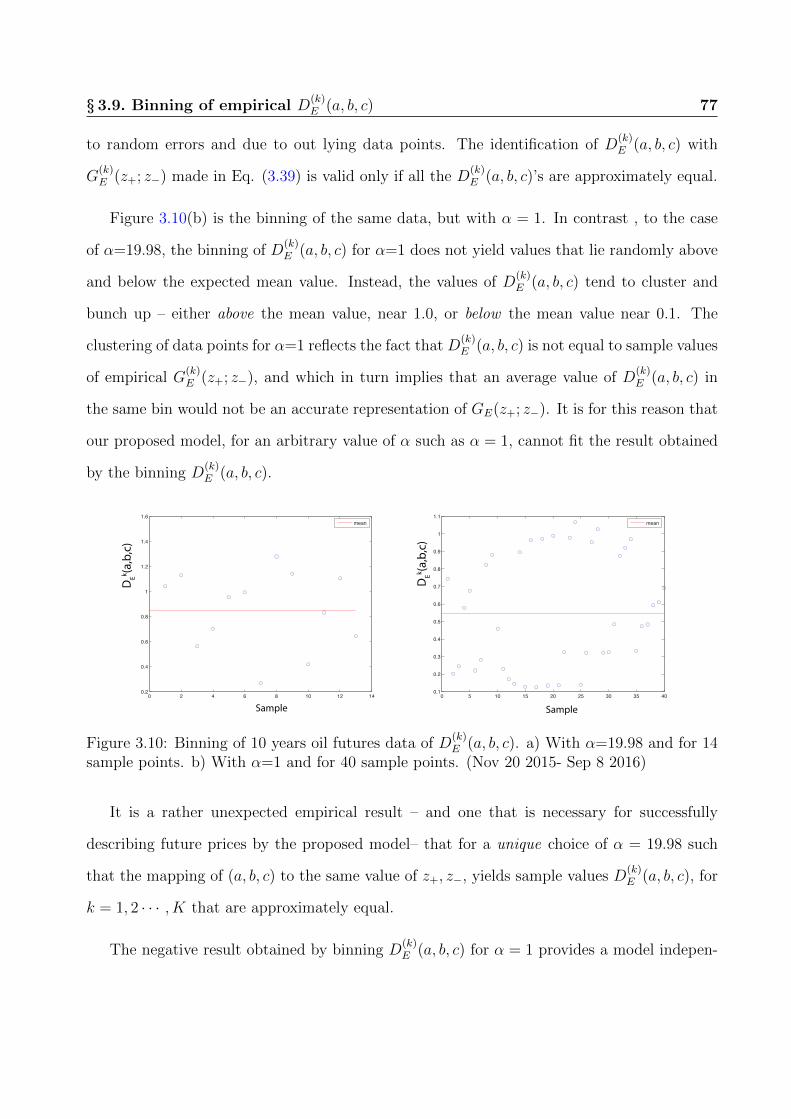
§ 3.9. Binning of empirical D(k)E (a, b, c) 77
to random errors and due to out lying data points. The identification of D(k)E (a, b, c) with
G(k)E (z+; z−) made in Eq. (3.39) is valid only if all the D
(k)E (a, b, c)’s are approximately equal.
Figure 3.10(b) is the binning of the same data, but with α = 1. In contrast , to the case
of α=19.98, the binning of D(k)E (a, b, c) for α=1 does not yield values that lie randomly above
and below the expected mean value. Instead, the values of D(k)E (a, b, c) tend to cluster and
bunch up – either above the mean value, near 1.0, or below the mean value near 0.1. The
clustering of data points for α=1 reflects the fact that D(k)E (a, b, c) is not equal to sample values
of empirical G(k)E (z+; z−), and which in turn implies that an average value of D
(k)E (a, b, c) in
the same bin would not be an accurate representation of GE(z+; z−). It is for this reason that
our proposed model, for an arbitrary value of α such as α = 1, cannot fit the result obtained
by the binning D(k)E (a, b, c).
0 2 4 6 8 10 12 140.2
0.4
0.6
0.8
1
1.2
1.4
1.6
mean
Sample
DE
k(a,b,c)
0 5 10 15 20 25 30 35 400.1
0.2
0.3
0.4
0.5
0.6
0.7
0.8
0.9
1
1.1
mean
DE
k(a,b,c)
Sample
Figure 3.10: Binning of 10 years oil futures data of D(k)E (a, b, c). a) With α=19.98 and for 14
sample points. b) With α=1 and for 40 sample points. (Nov 20 2015- Sep 8 2016)
It is a rather unexpected empirical result – and one that is necessary for successfully
describing future prices by the proposed model– that for a unique choice of α = 19.98 such
that the mapping of (a, b, c) to the same value of z+, z−, yields sample values D(k)E (a, b, c), for
k = 1, 2 · · · , K that are approximately equal.
The negative result obtained by binning D(k)E (a, b, c) for α = 1 provides a model indepen-

§ 3.10. Empirical results for GE(z+; z−) 78
dent test of the validity of the specific Lagrangian chosen in this chapter. By choosing an
arbitrary α and evaluating the value of the propagators for fixed values of (z+, z−), Figure
3.10(b) shows that for an arbitrary α the values of D(k)E (a, b, c) do not show the reduction of
the number of variables from a, b, c to (z+, z−): the values of D(k)E (a, b, c) are not approximately
equal.
One can do a model independent variation of α to determine the optimum α for which
the binning from a, b, c to (z+, z−) effectively results in a D(k)E (a, b, c) that is approximately a
constant; in this case, an optimum α would be a completely model independent result. It is
of course the expectation from the model that the model independent result for optimum α
would be close to the one obtained from the model.
In summary, Figure 3.10(a) provides reasonable evidence that there is a unique α for which
the binning yields an approximately constant value for DE(a, b, c); hence, one can conclude
that there exists a parameter α that encodes an inherent and model independent property of
the market’s behavior. The choice of α = 19.98 is guided by the requirement of obtaining the
best fit of the empirical propagator with the model’s propagator.
§ 3.10 Empirical results for GE(z+; z−)
The value of GE(z+; z−) for different values of z+, z− is shown in Figure 3.11(a), with the best
fit for the model’s G(z+; z−) shown in Figure 3.11(b). Given the complexity of the fit, a value
of R2 = 0.695 is reasonable. A more computationally intensive study needs to be carried out
for determining GE(z+; z−) more accurately.
The results of the calibration and fitting of the model are summarized in Table 3.2. The
calibration of the model has three distinct sources, namely the correlation function for (a)
spot-spot prices, (b) spot-futures prices and (c) futures-futures prices.

§ 3.10. Empirical results for GE(z+; z−) 79
0 2 4 6 8 10 12 14 160
10
20
−3
−2.5
−2
−1.5
−1
−0.5
0
0.5
1
1.5
0 2 4 6 8 10 12 14 16
0
5
10
15
20
−2
−1.5
−1
−0.5
0
0.5
1
1.5
2
Figure 3.11: a) Empirical GE(z+; z−) and b) Model GE(z+; z−) for market Oil futures prices.(Nov 20 2015- Sep 8 2016)
• Calibration using the spot-spot correlation function yields values consistent with the
results given in Table 3.1. The value of α is approximately 1 since it does not appear in
the spot-spot propagator G(t, t; t′, t′).
• The spot-future results for oil are also similar to the one obtained in Table 3.1. The
value of α is approximately 10.
• The value of L for the results given in Table 3.1 and Table 3.2 are very different, by
a factor of almost 1000 for spot-spot and spot-futures results. It is not clear why the
value of L should differ so much. Tables 3.1 and 3.2 refer to two different periods of
time, Jan 1 2011- Oct 18 2011 and Nov 20 2015- Sep 8 2016, receptively. It is possible
that the value of L has changed so dramatically due to the different periods used for
the calibration.
• The value of α = 19.98 is highest for the futures-futures case, as can be seen from Table
3.2. The reason, from the discussion in Section § 3.5, is that the highest contributions
to the propagator is only futures prices which are far in the future.
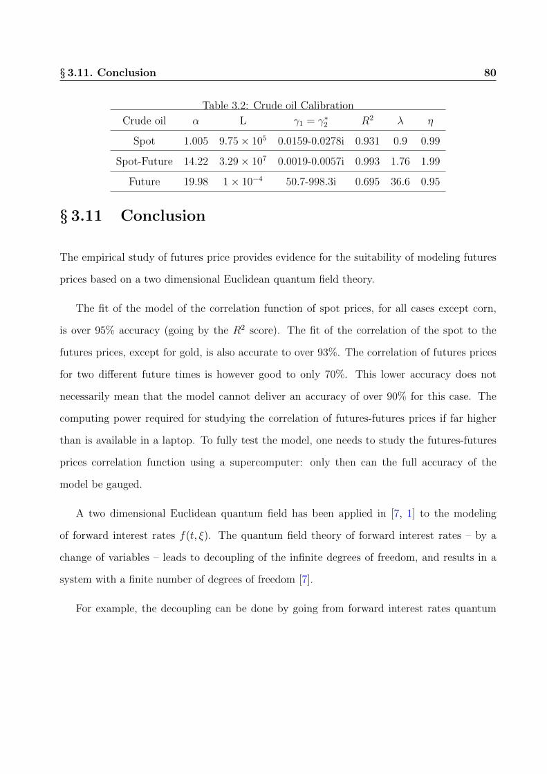
§ 3.11. Conclusion 80
Table 3.2: Crude oil Calibration
Crude oil α L γ1 = γ∗2 R2 λ η
Spot 1.005 9.75× 10⁵ 0.0159-0.0278i 0.931 0.9 0.99
Spot-Future 14.22 3.29× 10⁷ 0.0019-0.0057i 0.993 1.76 1.99
Future 19.98 1× 10⁻⁴ 50.7-998.3i 0.695 36.6 0.95
§ 3.11 Conclusion
The empirical study of futures price provides evidence for the suitability of modeling futures
prices based on a two dimensional Euclidean quantum field theory.
The fit of the model of the correlation function of spot prices, for all cases except corn,
is over 95% accuracy (going by the R2 score). The fit of the correlation of the spot to the
futures prices, except for gold, is also accurate to over 93%. The correlation of futures prices
for two different future times is however good to only 70%. This lower accuracy does not
necessarily mean that the model cannot deliver an accuracy of over 90% for this case. The
computing power required for studying the correlation of futures-futures prices if far higher
than is available in a laptop. To fully test the model, one needs to study the futures-futures
prices correlation function using a supercomputer: only then can the full accuracy of the
model be gauged.
A two dimensional Euclidean quantum field has been applied in [7, 1] to the modeling
of forward interest rates f(t, ξ). The quantum field theory of forward interest rates – by a
change of variables – leads to decoupling of the infinite degrees of freedom, and results in a
system with a finite number of degrees of freedom [7].
For example, the decoupling can be done by going from forward interest rates quantum

§ 3.11. Conclusion 81
field f(t, ξ) to a two dimensional quantum field A(t, ξ) by the following change of variables
∂f(t, ξ)
∂t= β(t, ξ) + σ(t, ξ)A(t, ξ)
where β(t, ξ), σ(t, ξ) are deterministic functions [1]. The quantum field A(t, ξ) is decoupled
in the time direction t and the action functional is effectively many copies (labeled by t) of a
quantum mechanical system, with role of ‘time’ being played by ξ.
If one moves from the path integral to the Hamiltonian, the degree of freedom is f(t, ξ) and
the infinitely many coupled degrees of freedom cannot be decoupled. But if one is interested
in only the correlation functions of f(t, ξ), then these are evaluated using the path integral
and the system is effectively quantum mechanical.
In contrast, the model for futures prices is an irreducible two dimensional nonlinear quan-
tum field. Due to the high order derivatives in the action functional, this theory is completely
finite. There is no need for the procedure of renormalization, which is necessary for obtaining
finite results from nonlinear quantum fields without the higher derivative term; these quantum
fields occur in high energy physics and in the theory of phase transitions.
Many questions remain, including studying the nonlinear terms of the model that are
required for determining the potential of the commodities that yield the futures prices. An-
other open question is the coupling of the futures prices of different commodities – and the
calibration and empirical tests for these models.
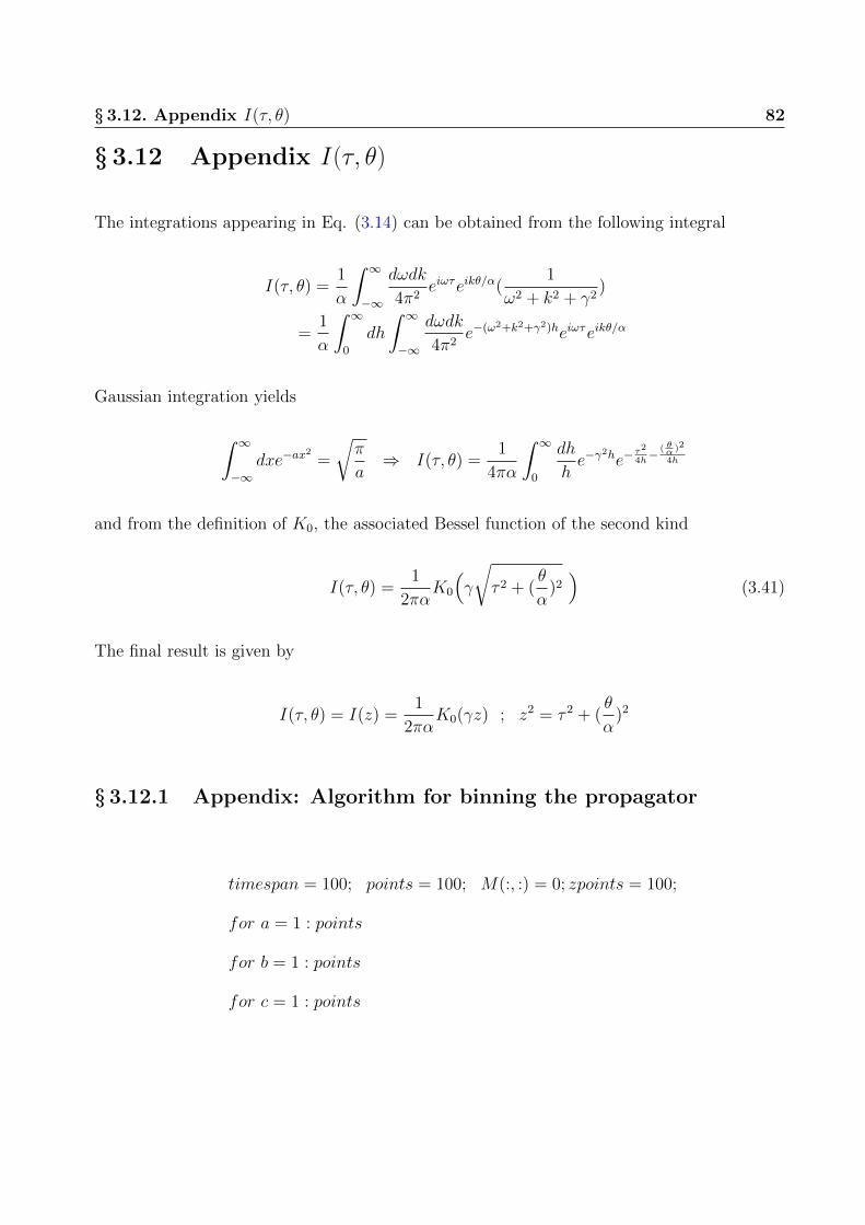
§ 3.12. Appendix I(τ, θ) 82
§ 3.12 Appendix I(τ, θ)
The integrations appearing in Eq. (3.14) can be obtained from the following integral
I(τ, θ) =1
α
∫ ∞−∞
dωdk
4π2eiωτeikθ/α(
1
ω2 + k2 + γ2)
=1
α
∫ ∞0
dh
∫ ∞−∞
dωdk
4π2e−(ω2+k2+γ2)heiωτeikθ/α
Gaussian integration yields
∫ ∞−∞
dxe−ax2
=
√π
a⇒ I(τ, θ) =
1
4πα
∫ ∞0
dh
he−γ
2he−τ2
4h− ( θα )2
4h
and from the definition of K0, the associated Bessel function of the second kind
I(τ, θ) =1
2παK0
(γ
√τ 2 + (
θ
α)2)
(3.41)
The final result is given by
I(τ, θ) = I(z) =1
2παK0(γz) ; z2 = τ 2 + (
θ
α)2
§ 3.12.1 Appendix: Algorithm for binning the propagator
timespan = 100; points = 100; M(:, :) = 0; zpoints = 100;
for a = 1 : points
for b = 1 : points
for c = 1 : points

§ 3.12. Appendix I(τ, θ) 83
n = 0;
D(a, b, c) = 0;
for t = 1 : timespan
t′ = t+ a;
x = t+ b;
x′ = c+ a+ t;
D(a, b, c) = D(a, b, c) +G(t, x; t′, x′);
[Note: transforming from (t, x; t′x′) to (t− t′, x− t, x′ − t′)]
n = n+ 1;
end
D(a, b, c) = D(a, b, c)/n;
z+ = round
(√a2 +
(b+ c)2
α2
)
z− = round
(√a2 +
(b− c)2
α2
)M(z+, z−) = M(z+, z−) + 1
GE(z+, z−,M(z+, z−)) = D(a, b, c);
end
end
end

§ 3.12. Appendix I(τ, θ) 84
for z+ = 1 : zpoints
for z− = 1 : zpoints
G(z+, z−) = 0;
for k = 1 : M(z+, z−)
G(z+, z−) = G(z+, z−) +GE(z+, z−, k);
end
G(z+, z−) = G(z+, z−)/M(z+, z−);
end
end

Chapter 4
Option Price and Market Instability
§ 4.1 Introduction
Baaquie introduced the action functional for pricing the Black-Scholes (BS) model in [7] and
the Black-Scholes price was given a path integral derivation starting from the action functional.
In 2014, Baaquie and Yang postulated another action functional for the option pricing; the
Baaquie and Yang (BY) option price depends on the stock price and its velocity – and is
essentially Gaussian since the action functional is quadratic in the logarithm of the security
(equity) or FX rate [5]. The BY model following the Gaussian model provides analytical
solution and explanation in comparison to Non-Gaussian model [30, 31].
The FX option for the exchange rate of various currencies against the US Dollar are studied
for the period from 2011 to 2015; the following behavior is observed.
• For all currencies, there are ‘normal’ periods where the BY model fits the data fairly
well.
• There are sudden intermittent periods that punctuate the normal period. And for these
periods, the model fails dramatically due to market instability.
• The volatility of the underlying FX rate is not a suitable as an indicator of market
85

§ 4.1. Introduction 86
instability.
Our hypothesis is that the failure of the BY model to fit market data is due to the effects
of instability that are not captured by the BY model since it is essentially Gaussian. This
simplicity of the BY model is used to our advantage by postulating that market instability
introduces nonlinear effects causing the model to fail. This very failure of the model in turn
is used as a barometer and as a gauge for concluding that the FX market has entered an
unstable and potentially a crisis phase.
The behavior of FX options is an accurate gauge of the state of the international financial
system. The FX markets are international and operate 24 hours a day – and are expected to
quickly respond to the changing tides of the major economic powers[32]. Furthermore, there
is a high volume of daily FX transaction: trading in foreign exchange markets averaged $5.3
trillion per day in April 20131. High liquidity and the key role of currencies in the major
economies, in our opinion, makes FX options a sensitive gauge of the international financial
system.
The industry bench mark for pricing European call option is based on the Black-Scholes
model. Let the price of security be S = ex. For concreteness, consider a vanilla call option
with a payoff function [ex − K]+ and maturing at some future time T . The option price in
general has the following time parameters
t : present calendar time ; T : maturity time ; τ : remaining time.
The BS option price is given by[33, 34, 35]
CBS(S(t), K, r, σ, (T − t)) = SN(d+)− e−r(T−t)KN(d−),
1https://en.wikipedia.org/wiki/Foreign exchange market.

§ 4.2. Quantum finance formulation 87
where
d± =ln(S/K) + r(T − t)± σ2
0(T − t)/2σ0
√(T − t)
; N(x) =1√2π
∫ x
−∞e−
12z2dz.
§ 4.2 Quantum finance formulation
Let x = dx/dt be the velocity of the logarithm of S. In general, the option price C can depend
on the price and velocity of the security. A payoff function H(x, v;K) can depend on both
the final stock value and velocity; for remaining time τ = T − t
C(x(t), x(t), τ,K) =
∫dxdx′P (x, x;x′, x′; τ)H(x′, x′;K),
where expression
P (x, x;x′, x′; τ).
is the conditional probability that the future value is x′, x′ at time T , given the value of x, x
at present time t. Furthermore, let
P (x, x;x′; τ) =
∫dx′P (x, x;x′, x′; τ),
where P (x, x;x′; τ) is the marginal conditional probability.
In the quantum finance formulation of option prices, the conditional probability P (x, x;x′, x′; τ)
is given by what is called the transition amplitude
K(x, x;x′, x′; τ).
The conditional probability P(x, x;x′, x′; τ) is given by appropriately normalizing the tran-

§ 4.2. Quantum finance formulation 88
sition amplitude and yields
P (x, x;x′, x′; τ) =K(x, x;x′, x′; τ)∫
dx′dx′K(x, x;x′, x′; τ),
P (x, x;x′; τ) =
∫dx′P (x, x;x′, x′; τ). (4.1)
The description of the stochastic evolution of a security is defined by the Hamiltonian H
operator for the security [7]. The transition amplitude, in general, is given by the matrix
element of the Hamiltonian operator [3]
K(x, x;x′, x′; τ) = 〈x, x|e−τH |x′, x′〉. (4.2)
The transition amplitude K(x, x;x′, x′;T, t) has another representation defined by the (Eu-
clidean) Feynman path integral over all possible paths x(t) of the security from its initial value
x′, x′ at time τ = 0 to its final value of x, x at time τ [3]. More precisely,
K =
∫DxeS . (4.3)
Up to a normalization, the path integral measure is given by
∫Dx =
τ∏t=0
∫ ∞−∞
dx(t).
The boundary conditions for all the allowed paths in the Feynman path integral given in Eq.
(4.3) is the following [36]
x(0) = x′, x(0) = x′; x(τ) = x, x(τ) = x. (4.4)

§ 4.3. Transition amplitude K 89
§ 4.3 Transition amplitude K
The model Hamiltonian H for the option price is given by [3]
H = − 1
2a
∂2
∂x2− x ∂
∂x+ bx2 +
1
2cx2. (4.5)
The Hamiltonian given in Eq. (4.5) yields the following ‘acceleration’ Lagrangian, derived in
[3] and given by
L = −1
2
(ax2 + 2b(x+ j)2 + cx2
); S =
∫ τ
0
dtL. (4.6)
Since the Lagrangian given in Eq. (4.6) is quadractic, the path integral can be solved
exactly using the classical solutions. The stochastic variable x is separated into two parts:
the classical solution xc and stochastic part ξ.
x = xc + ξ (4.7)
with the classical solution xc given by
δS[xc]
δx(t)= 0.
The classical solution has boundary conditions as Eq. (4.4) and we hence obtain
xc(0) = x′, xc(0) = x′; xc(τ) = x, xc(τ) = x. (4.8)
Hence, Eqs. (4.7) and (4.8) yield the boundary condition as below
ξ(0) = 0; ξ(τ) = 0; ξ(0) = 0; ξ(τ) = 0. (4.9)

§ 4.4. BY Model option price 90
The acceleration action S separates into two parts [5] and is given by
S = S[xc] + S[ξ]. (4.10)
Note S[ξ] is independent of x, x, x′, x′ and depends only on τ . The transition amplitude is
given by
K =
∫DxeS =
∫DξeSξ+Sc = N eSc . (4.11)
The functional integration is defined by
∫Dx =
τ∏t=0
∫ ∞−∞
dx(t) ;
∫Dξ =
τ∏t=0
∫ ∞−∞
dξ(t),
and the normalization is given by
N (τ) =
∫DξeSξ .
We obtain the final result that
K(x, x;x′, x′; τ) = N (τ) expSc(x, x;x′, x′; τ). (4.12)
§ 4.4 BY Model option price
The BY (Baaquie-Yang) model for option pricing – proposed in [37] – is based on the La-
grangian and action given in Eq. (4.6), and is unlike the Black-Scholes case. The BY price
for the European call option, at time t, is given by
CBY (x(t), x(t), τ,K) =
∫dx′P (x, x;x′; τ)[ex
′ −K]+.

§ 4.4. BY Model option price 91
Since the Lagrangian and action S[xc] given by Eq. (4.6) yields [3]
S[xc] = −1
2
∫ τ
0
dt(ax2c + 2b(xc + j)2 + cx2
c). (4.13)
The classical solution S[xc] with the boundary condition Eq. (4.4) is solved in the Appendix
§ 4.11.1. The conditional possibility is given by Eq. (4.59)
P (x, x;x′; τ) =
∫dv′P (x, x;x′, x′; τ) =
√1
2πν2exp− 1
2ν2(−x′ + ζx+ ξx+ j)
2.
The solution for the classical action Sc yields the following
ν2 =2Ωrω[ω sinh(2rτ)− r sin(2ωτ)]
a (r2 + ω2),
ζ = 4Ωrω[(r2 − ω2
)sinh(rτ) sin(ωτ) + 2rω cosh(rτ) cos(ωτ)],
ξ = −4Ωrω[ω sinh(rτ) cos(ωτ) + r cosh(rτ) sin(ωτ)], (4.14)
where
Ω =1
(r2 + ω2)2 − r2 (r2 − 3ω2) cos(2ωτ)− ω2 (ω2 − 3r2) cosh(2rτ). (4.15)
r and ω are defined in the Appendix Eq. (4.42) and given below
r ≡ Re
√b+ i√ac− b2
a
; ω ≡ Im
√b+ i√ac− b2
a
.
Some typical shapes of ν2, ξ, ζ, as a function of τ , are shown in Figures 4.1, 4.2, 4.3 and
4.4.

§ 4.4. BY Model option price 92
0 0.5 1 1.5 2 2.5 30
0.005
0.01
0.015
0.02
τ(year)
ν2
Figure 4.1: ν2(τ)
0 0.5 1 1.5 2 2.5 30
0.02
0.04
0.06
0.08
0.1
0.12
0.14
τ(year)
Figure 4.2:√ν2/τ
0 0.5 1 1.5 2 2.5 3−0.4
−0.35
−0.3
−0.25
−0.2
−0.15
−0.1
−0.05
0
0.05
τ(year)
Figure 4.3: ξ(τ)
0 0.5 1 1.5 2 2.5 3−0.2
0
0.2
0.4
0.6
0.8
1
1.2
τ(year)
Figure 4.4: ζ(τ)
Figure 4.5: Shape of parameters with a = 5; b = 8; c = 100. τ is remaining time.
§ 4.4.1 Martingale condition
Consider the case of FX options. Let the domestic currency be $ and the value of a foreign
currency is given by $ex. and let rf and rd be the risk free foreign and the domestic interest
rates, respectively. As discussed in [5], the Forex option martingale condition[38] is given by
e−rf τex = e−rdτ∫ +∞
−∞dx′P(x, x;x′; τ)ex
′. (4.16)
The Forex exchange martingale process is shown by Fig. 4.6
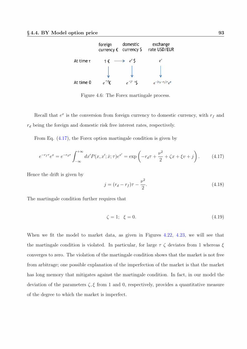
§ 4.4. BY Model option price 93
Figure 4.6: The Forex martingale process.
Recall that ex is the conversion from foreign currency to domestic currency, with rf and
rd being the foreign and domestic risk free interest rates, respectively.
From Eq. (4.17), the Forex option martingale condition is given by
e−rf τex = e−rdτ∫ +∞
−∞dx′P (x, x′; x; τ)ex
′= exp
(−rdτ +
ν2
2+ ζx+ ξv + j
). (4.17)
Hence the drift is given by
j = (rd − rf )τ −ν2
2. (4.18)
The martingale condition further requires that
ζ = 1; ξ = 0. (4.19)
When we fit the model to market data, as given in Figures 4.22, 4.23, we will see that
the martingale condition is violated. In particular, for large τ ζ deviates from 1 whereas ξ
converges to zero. The violation of the martingale condition shows that the market is not free
from arbitrage; one possible explanation of the imperfection of the market is that the market
has long memory that mitigates against the martingale condition. In fact, in our model the
deviation of the parameters ζ, ξ from 1 and 0, respectively, provides a quantitative measure
of the degree to which the market is imperfect.

§ 4.4. BY Model option price 94
§ 4.4.2 BY Option: market time
The FX call option BY price CBY (x, x;K, τ) is given by
CBY (x, x; τ,K) = e−rdτ∫ +∞
−∞dx′P (x, x′; x; τ)
[ex′ −K
]+
= e−rf τeζx+ξxN(d+)− e−rdτKN(d−),
where d± =ζx+ ξx− ln(K) + (rd − rf )τ ± ν2
2
ν.
We introduce two new parameter λ and η such that
t→ z = λ(t
λ)η. (4.20)
The function z(t) [7] is called market time to differentiate it from calendar time t. Market
time is the subjetive estimate of time in the minds of the traders whereas calendar time is
physical time. The parameters λ, η is a measure of market time, which is greater than calendar
time for t < λ and less for t > λ. The difference between t and z, when η < 1, is shown in
Figure 4.7.
0
y
t
y=t
y=
Figure 4.7: The t and z values when η < 1
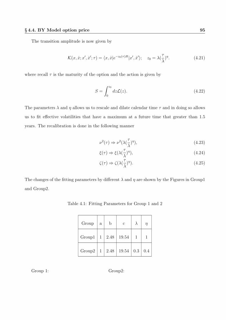
§ 4.4. BY Model option price 95
The transition amplitude is now given by
K(x, x;x′, x′; τ) = 〈x, x|e−z0(τ)H |x′, x′〉; z0 = λ(τ
λ)η. (4.21)
where recall τ is the maturity of the option and the action is given by
S =
∫ z0
0
dzL(z). (4.22)
The parameters λ and η allows us to rescale and dilate calendar time τ and in doing so allows
us to fit effective volatilities that have a maximum at a future time that greater than 1.5
years. The recalibration is done in the following manner
ν2(τ)⇒ ν2(λ(τ
λ)η), (4.23)
ξ(τ)⇒ ξ(λ(τ
λ)η), (4.24)
ζ(τ)⇒ ζ(λ(τ
λ)η). (4.25)
The changes of the fitting parameters by different λ and η are shown by the Figures in Group1
and Group2.
Table 4.1: Fitting Parameters for Group 1 and 2
Group a b c λ η
Group1 1 2.48 19.54 1 1
Group2 1 2.48 19.54 0.3 0.4
Group 1: Group2:

§ 4.4. BY Model option price 96
0 500 1000 1500 2000 2500 30000
0.01
0.02
0.03
0.04
0.05
0.06
0.07
0.08
0.09
Figure 4.8: ν2(z) for Group 1
0 0.5 1 1.5 2 2.5 30
0.01
0.02
0.03
0.04
0.05
ν2
τ(year)
Figure 4.9: ν2(z) for Group 2
0 500 1000 1500 2000 2500 3000−0.35
−0.3
−0.25
−0.2
−0.15
−0.1
−0.05
0
0.05
Figure 4.10: ξ(z) for Group 1
0 0.5 1 1.5 2 2.5 3−0.35
−0.3
−0.25
−0.2
−0.15
−0.1
−0.05
0
τ(year)
Figure 4.11: ξ(z) for Group 2
0 500 1000 1500 2000 2500 3000−0.2
0
0.2
0.4
0.6
0.8
1
1.2
Figure 4.12: ζ(z) for Group 1
0 0.5 1 1.5 2 2.5 30.7
0.75
0.8
0.85
0.9
0.95
1
τ(year)
Figure 4.13: ζ(z) for Group 2
It is obvious that when λ and η change from [1, 1] to [0.3, 0.4], the shape of the parameters

§ 4.5. Mapping BY Model to data 97
[µ, ξ, ζ] also varies significantly. For example, Figures. 4.16 and 4.17 can be fit very well with
λ = 1, but it is graphs of the type shown in Figure 4.18 that can only be fitted by the model
with λ 6= 1.
§ 4.5 Mapping BY Model to data
Every option has a remaining time τ = T − t; the option price is studied for a fixed remaining
time τ . Options can be studied for which remaining time τ remains constant, namely a
collection of options issued at different calendar time and maturing at a constant time in the
future. Another class of options is having a maturity time at some fixed calendar τ = T − t,
for which T is held fixed. Both these options are shown in Figure 4.14. In this chapter, we
find the options for which τ is held fixed, which is even complicated than the LIBOR market
[39].
For each instant t, the value of the security is represented by the model variable x(z(τ)).
To make the mapping of the model variables to market data more clear, let t be calendar time
and x = τ + t be the future time, as shown in Figure 4.14(a). We adopt the notation that
x(z) = x(t, z(τ)) : z(τ) = λ(τ
λ)η ; τ = x− t : constant τ
For the case of options with remaining time τ that is fixed, as shown in Figure 4.14(a), the
notation x(t, z(τ)) means the value of the stock price at time t for an option maturing at
future time t + τ . For options that mature at some fixed time T in the future, as shown in
Figure 4.14(b), we have the notation
x(z) = x(t, z(T − t)) : z(τ) = λ(T − tλ
)η ; τ = T − t : constant T

§ 4.5. Mapping BY Model to data 98
future time0
x(t’,τ)
x(t,τ)
t’
t
τ
t(calendar time)
future time0
t’
t
T
T
(a) (b)
x(t’,τ)
x(t,τ)
x(t’,τ(t’))
x(t,τ(t))
t(calendar time)
Figure 4.14: (a) The model variable x(t, τ) with different calendar times t, t′ but with thesame remaining time τ . (b) Model variable for fixed maturity time T , with remaining timeτ(t) 6= τ(t′).
Let xD(t) be the value of the data at time t. The calibration of the model is based on the
following mapping
xD(t) = x(t, z(τ)) : constant τ (4.26)
xD(t) = x(t, z(T − t)) : constant T (4.27)
The mapping from t to z, and the connection of data xD(t) to its representation in the model
x(z(t)), is shown in Figure 4.15. Eqs. (4.26) and (4.27) may look a bit strange since xD(t)
does not depend on τ ; the role played by τ in mapping the model to data will become more
clear when we compute the velocity of the model.
The velocity in the model is defined by
dx
dz=dt
dz
dx
dt.

§ 4.5. Mapping BY Model to data 99
From the definition of market time we have
dz
dt=
d
dt
(λ(x− tλ
)η)
= −η(τ
λ)η−1.
To relate the model velocity to the velocity given by data, we compare the value of data at
two nearby instants given by t and t− δ – as shown in Figure 4.15. For fixed remaining time
τ , as shown in Figure 4.15(a), we have the following
dx(t, z(τ))
dz=
(−η(
τ
λ)η−1
)−1 dx(z)
dt
=(−η(
τ
λ)η−1
)−1 x(t, z(τ))− x(t− δ, z(τ))
δ.
From the mapping given in Eq. (4.26) we obtain
dx
dz= −1
η
(τλ
)1−η· xD(t)− xD(t− δ)
δ. (4.28)
In the analysis of this chapter δ is chosen equal to 1 day=1/360 years.
. . . . . .
xD(t-δ))=x(t-δ,τ)
t
. . . . . .
x(T,Z(τ))
x(T,Z(T-t+δ))ε
(a) (b)
xD(t-δ))=x(t-δ,τ)
xD(t)=x(t,τ)xD(t)=x(t,τ)t
t-δ t-δx(t-δ,τ)
0 0T1 T1
t(calendar time) t(calendar time)
future time future time
Figure 4.15: (a) Model velocity for fixed remaining time τ . (b) Model velocity for fixedmaturity time T is found by comparing x(t, z(τ) to x(t− δ, z(τ + δ).

§ 4.5. Mapping BY Model to data 100
The mapping for the option with fixed maturity time T is given in Eq. (4.27) and yields
dx
dz=
x(t, z(T − t))− x(t− δ, z(T − t)− ε)ε
=xD(t)− xD(t− δ)
ε(4.29)
ε = λ(τ
λ)η − λ(
τ + δ
λ)η = −η(
τ
λ)η−1δ +O(δ2) : τ = T − t
where ε is shown in Figure 4.15(b). From Eq. (4.29), note that a change of δ in calendar time
is equal to a change of ε in market time z(T − t).
Note that the result given in Eq. (4.29) for an option with a fixed maturity T is the same
as the result for constant remaining time τ given in Eq. (4.28).
The mapping of the model velocity to data is given in Eq. (4.28). Note that dx/dz is the
velocity for an option maturing after remaining time τ , as shown in Figure 4.15. The options
for different remaining times have the empirical velocity dxD/dt scaled by the remaining time
τ for obtaining the effective model velocity dx/dz. The scaling factor is the same for options
with constant remaining time and with a fixed maturity time, and is the following
1
η
(τλ
)1−η.
Since η < 1 we see that the model’s velocity is enhanced for large remaining time τ , with the
effect of market time become more significant for τ >> λ.
Note for η → 1, z(τ) → τ , and hence market time becomes equal to remaining calendar
time, and the scaling factor becomes 1 as expected.

§ 4.6. Calibration of the BY Model 101
§ 4.6 Calibration of the BY Model
The fitting of the data is with the price of call option given by Eq. (4.20) 2
Cdata(τ) = CBY (rf , rd, z(τ), x, x). (4.30)
The market price Cdata is obtained from the Black-Sholes formula
Cdata(τ) = CBS(S,K, rf , rd, σATM , T − t0). (4.31)
Where σATM is provided by the market. The testing and calibration is given by using
Eqs. (4.30) and (4.31).
The at-the-money (ATM) options are often used to calculate the implied volatility because
they are the most traded contracts; implied volatility differs with strike prices and time to
expiration as well as depending on calendar time. We use the data from Bloomberg to obtain
implied volatility σATM in the form of a dimensionless number τG2data(τ), with at-the-money
implied volatility given by
σATM =√τG2
data(τ).
The FX volatility data is downloaded from Bloomberg and the following moving remaining
times are chosen as
τn|n = 1, 2, ...8 = [0.0833, 0.1667, 0.25, 0.5, 1, 1.5, 2, 3] years.
2The calibration of the model in [5] is for market ATM volatility Gdata and uses the formula
ν2(τη) = G2data(τ)τ
The shortcoming of this calibration is that the parameters λ is not used. This leads to the maximum of theeffective volatility in the paper being fixed to be at around 1.5 years in the future, and hence is unable to fitmany cases.

§ 4.7. Fitting Results 102
R-square and root mean square (RMSE) error are chosen to measure the goodness of fit. For
each calendar date t, there is a fit of volatility Cdata, so the R-square and RMSE error are
functions of calendar time t. R2 is defined as
R2(t) = 1−
8∑n=1
[Cdata(t, τn)− Cfit(t, τn)]2
8∑n=1
[Cdata(t, τn)− Cdata(t, τn)]2
. (4.32)
where τn is the remaining time and Cdata(t, τn) is the mean of Cdata(t) at calendar time t.
Higher R2 means better fit, and the exact fit has an R2 value equal to 1.
RMS error is defined by
RMSE(t) =
√√√√ 1
N
N∑n=1
[Cdata(t, τn)− Cfit(t, τn)
Cdata(t, τn)
]2
. (4.33)
§ 4.7 Fitting Results
In general, the data results in three typical shapes that can be fitted by the model and irregular
shapes that have no fit. The pattern C is in fact the same as pattern A; with the difference
that for pattern C the maximum has been pushed out far into the future. Pattern C can be
fitted by choosing a suitable λ.
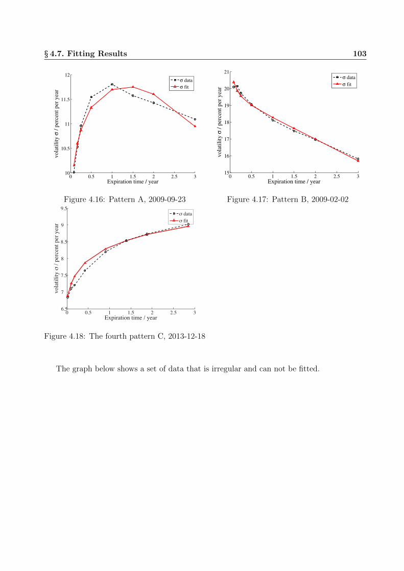
§ 4.7. Fitting Results 103
0 0.5 1 1.5 2 2.5 310
10.5
11
11.5
12
Expiration time / year
vola
tili
ty σ
/ p
erce
nt
per
yea
r
σ data
σ fit
Figure 4.16: Pattern A, 2009-09-23
0 0.5 1 1.5 2 2.5 315
16
17
18
19
20
21
Expiration time / year
vola
tili
ty σ
/ p
erce
nt
per
yea
r
σ data
σ fit
Figure 4.17: Pattern B, 2009-02-02
0 0.5 1 1.5 2 2.5 36.5
7
7.5
8
8.5
9
9.5
Expiration time / year
vo
lati
lity
σ /
per
cen
t p
er y
ear
σ data
σ fit
Figure 4.18: The fourth pattern C, 2013-12-18
The graph below shows a set of data that is irregular and can not be fitted.

§ 4.7. Fitting Results 104
0 0.5 1 1.5 2 2.5 310.3
10.32
10.34
10.36
10.38
10.4
10.42
10.44
10.46
10.48
Expiration time / year
vo
lati
lity
σ /
per
cen
t p
er y
ear
σ data
σ fit
Figure 4.19: Irregular data, 2008-08-28
The model has five free parameters, as shown in Table 1, and options with 8 different
remaining time are being fitted. The fits are usually very good, except for exceptional periods.
To test our hypothesis, we mark those periods for which the fit fails, namely for which R2 <
0.99.
We analyze the exchange rate of the major international currencies against the US Dollar,
namely the Euro, the Pound (GBP), the Japanese Yen, the Swiss Franc (CHF), the Australian
Dollar (AUD), the Canadian Dollar and the New Zealand Dollar.
Of these we analyze the option of the exchange rate of five major currencies against the US
Dollar, which are the Euro, GBP, CHF, Yen, AUD. The Canadian Dollar is highly correlated
with the US Dollar and the New Zealand Dollar to the AUD, and hence their analysis does
not give any new insights.
The scheme of our analysis is the following.
• We find the periods for which the model fails.
• We seek to explain the reason of their failure as being due to market turbulence.
• If the failure of model for a time period occurs only for a particular a country, we look

§ 4.7. Fitting Results 105
for reasons such as policy changes or international developments that specifically impact
on that country.
• If for a time period the model fails for all the major currencies, we seek an explanation
that originates in the international financial system.
The graphs below shows one example of the EURUSD fitting at 2, January, 2008.
Table 4.2: Parameters for EURUSD Fitting
R2 a b c λ η
0.9992 23.96 0.801 2.48 0.843 0.325

§ 4.7. Fitting Results 106
0 0.5 1 1.5 2 2.5 30.02
0.03
0.04
0.05
0.06
0.07
0.08
0.09
0.1
0.11
data
fit
(year)Remaining time
Figure 4.20: Option price fitting
0 0.5 1 1.5 2 2.5 30
0.005
0.01
0.015
0.02
0.025
0.03
0.035
(year)
Remaining time
Figure 4.21: ν2
0 0.5 1 1.5 2 2.5 3−1.5
−1.4
−1.3
−1.2
−1.1
−1
−0.9
−0.8
−0.7
−0.6
−0.5
(year)
Remaining time
Figure 4.22: ξ
0 0.5 1 1.5 2 2.5 30.994
0.995
0.996
0.997
0.998
0.999
1
1.001
(year)Remaining time
Figure 4.23: ζ

§ 4.7. Fitting Results 107
The graphs below shows the parameters fitting for EURUSD from 2009/01/01 to 2009/04/21.
0 10 20 30 40 50 60 700.9997
0.9997
0.9998
0.9998
0.9999
0.9999
1
time lag(day)
Figure 4.24: Option price fitting R2
0 10 20 30 40 50 60 702
3
4
5
x 10−4
time lag(day)
Figure 4.25: Option fitting rmse
0 10 20 30 40 50 60 700
0.1
0.2
0.3
0.4
0.5
0.6
0.7
time lag(day)
Figure 4.26: r
0 10 20 30 40 50 60 700
0.05
0.1
0.15
0.2
0.25
0.3
0.35
0.4
0.45
0.5
time lag(day)
Figure 4.27: ω
0 10 20 30 40 50 60 700.5
1
1.5
2
2.5
3
time lag(day)
Figure 4.28: λ
0 10 20 30 40 50 60 700.32
0.34
0.36
0.38
0.4
0.42
0.44
0.46
(time lag(day)
Figure 4.29: η

§ 4.8. Global crisis 108
§ 4.8 Global crisis
Our focus is from 2008 to the present (2016). Before embarking on a study of specific cur-
rencies, we expect that events that have had a major impact on the international financial
system should be enumerated and we should be able to find signals of these globally. This
would provide a check on our analysis as well as show the consistency of using FX option
price as a gauge of the international financial system.
Two international events with a potentially significant impact on almost all countries of
the world are discussed below.
• The period of international significance is the 2007-2008 financial crisis – that is indicated
by dashed lines for all the currencies.3
Figure 4.30: TED and the financial crisis in 2008.4
The TED spread is an acronym for the difference between the interest rates on interbank
loans and on short-term U.S. government debt. The TED spread is calculated in the
3https://en.wikipedia.org/wiki/Financial crisis of 2007%E2%80%9308.

§ 4.8. Global crisis 109
market by measuring the difference between the three-month LIBOR and the three-
month US Treasury-bills interest rate. A large TED spread indicates an increase in
the risk of short term commercial loans and a lack of liquidity. The sudden spike in
TED reaching almost 5%, as shown in Figure 4.30 (where USGG3M is the US 3-month
treasury bill), is a reflection of the 2008 financial meltdown.
The model in [5] showed that the Euro FX option price data could also be used to gauge
the market. The model could correctly reflect the occurrence of the global financial crisis
on the EURUSD exchange rate. This result is re-produced in Figure 4.31 and indicated
by I.
• We examine the impact of the 2007-2008 financial separately for the five major curren-
cies.
• United States debt-ceiling crisis of 2013 lasted January-October, 2013. 5 Our study
shows that the crisis had a strong impact on Europe and Japan but little impact on
Australia and Switzerland; this is because both Australia and Switzerland are not that
closely tied to the US financial policy as are Europe and Japan.
• According to our model based on the pricing of FX options for 2014-2015, the Euro,
British and Swiss Franc were impacted by the drastic fall in oil-prices and the deterio-
ration of the relation of the US and Europe with Russian.
• The black swan event for the Swiss Franc was caused internally by removing the pegging
of the Swiss Franc to the Euro.
Our study also shows many other instabilities, some of which are country specific.
5https://en.wikipedia.org/wiki/United States debt-ceiling crisis of 2013.

§ 4.9. Result for five major FX options 110
§ 4.9 Result for five major FX options
From the graphs we can see that all of Europe except the Swiss Franc were heavily influenced
by the 2008 financial crisis. Each graph for the FX options is alongside another graph showing
the volatility of the FX rate. We compare these graphs to see if the FX volatility is also an
accurate gauge of market instability. We find that the volatility of the FX rate is not a very
precise criterion of financial instability. For example, as shown in Fig. 4.31 (b), although
FX rate had a high volatility during the 2008 financial crisis, there are other periods of large
volatility with apparently no market instability.
§ 4.9.1 Euro
2008 2009 2010 2011 2012 2013 2014 2015 Date(year)0
50
100
150
200
250
300
350
400
450
500
2
0.975
0.98
0.985
0.99
0.995
1
1.005
2008 2009 2010 2011 2012 2013 2014 2015
Op
tio
n p
rice
R2
Date(year)
(a) (b)
(I) (II)
Ex
ch
an
ge
Vo
lati
lity
Figure 4.31: (a) R2 of EURUSD and (b) Fx volatility of EURUSD
The price of EURUSD option was disordered for a short period after the 2008 financial crisis.
The 2008 financial crisis, however, triggered sovereign debt crisis in Europe in 2013, and this
is marked as II in Figure 4.31. The crisis denoted by II could also have had contributions
from the US financial crisis of 2013. Hence, financial instability was correctly gauged by the
failure of the model.

§ 4.9. Result for five major FX options 111
§ 4.9.2 Australia Dollar
2008 2009 2010 2011 2012 2013 2014 2015 Date(year)0
80
160
240
320
400
480
560
640
720
800
2
Date(year)0
0.1
0.2
0.3
0.4
0.5
0.6
0.7
0.8
0.9
1
2008 2009 2010 2011 2012 2013 2014 2015
Op
tio
n p
rice
R2
(a) (b)E
xc
ha
ng
e V
ola
tili
ty
Figure 4.32: (a) R2 of AUDUSD and (b) Fx volatility of AUDUSD
The graph shows that for the period of the 2008 crisis, the model correctly reflects the financial
meltdown.
§ 4.9.3 Swiss Franc
2008 2009 2010 2011 2012 2013 2014 2015 Date(year)0
50
100
150
200
250
300
350
400
450
500
2
0.75
0.8
0.85
0.9
0.95
1
2008 2009 2010 2011 2012 2013 2014 2015 Date(year)
Op
tio
n p
rice
R2
(a) (b)
(I)
(II)
Ex
ch
an
ge
Vo
lati
lity
Figure 4.33: (a) R2 of CHFUSD and (b) Fx volatility of CHFUSD

§ 4.9. Result for five major FX options 112
The behavior of the model for the case of the Swiss Franc is one of the most interesting.
To start with, the 2007-2008 financial crisis left the Swiss Franc untouched since it did not
take part in the leveraging and high risk instruments that primarily the US and UK banks,
and to a lesser extent the European banks were engaged in. The fittings above confirms
our expectation that the Swiss Franc was not affected much in 2008; in constrast, the Euro,
including the British Pound, were highly impacted.
The Swiss dollar has a very big FX volatility from 2010 to 2012 as shown in Fig 4.33 (b).
This is because of a policy of the Swiss government. After the crisis broke out in 2008, there
was a flight to safety in Europe, with large flows of money to Swiss Bank. This raised the
value of the Swiss Franc and led to the Swiss policy, announced in September 2011, that set
an upper limit to the valuation of the CHF to EURO to be capped at 1.2. So the fluctuations
marked II in Figure 4.33(b) describes this high volatility period.
In 2015,January, 15th, the Swiss suddenly canceled the upper limit of CHF against the
Euro, which is a rare and unpredictable event and can be called a ”Black Swan” event. This
rare event is correctly captured by the failure of the model, and is marked by I in Figure
4.33(a).

§ 4.9. Result for five major FX options 113
§ 4.9.4 British Pound
2008 2009 2010 2011 2012 2013 2014 2015 Date(year)0
50
100
150
200
250
300
350
400
450
500
22008 2009 2010 2011 2012 2013 2014 2015 Date(year)
0.95
0.955
0.96
0.965
0.97
0.975
0.98
0.985
0.99
0.995
1
Op
tio
n p
ric
e R
2
(a) (b)
Ex
ch
an
ge
Vo
lati
lity
Figure 4.34: (a) R2 of GBPUSD and (b) Fx volatility of GBPUSD
The British Pound, as can be seen from Figure 4.34, was highly unstable in 2007 leading to the
crash of 2008. This is because it is closely tied to the behavior of the US Dollar. The British
Pound was fairly stable after 2008, becoming unstable in 2013-2014. It is relatively stable
now, compared to other major currencies. The volatility of the FX rate does not provide
any sign of instability, in contrast to the instability shown by the failure of the model for the
period of 2013 and end of 2014.

§ 4.10. Conclusion 114
§ 4.9.5 Japanese Yen
2008 2009 2010 2011 2012 2013 2014 2015 Date(year)0
50
100
150
200
250
300
350
400
450
500
Ex
ch
an
ge
Vo
lati
lity
2
Date(year)0.93
0.94
0.95
0.96
0.97
0.98
0.99
1
2008 2009 2010 2011 2012 2013 2014 2015
Op
tio
n p
rice
R2
(a) (b)
Figure 4.35: (a) R2 of JPYUSD and (b) Fx volatility of JPYUSD
According to Figures 4.31(a) and 4.34(a), from 2008 to 2009, the EUR and GBP has imme-
diately disordered when the crisis of 2007-2008 occurred. The Japanese Yuan option, as seen
in Figures 4.35, was immediately affected between 2009 and 2010. This fact seems to show
that although Japan has the same financial policy as the Western countries, the crisis had a
delayed effect on Japan.
§ 4.10 Conclusion
The model for FX options is based on a Gaussian Lagrangian. The hypothesis that the option
price cannot fit the market’s behavior when the market is undergoing large scale fluctuations
and changes seems to be borne out by data. The accuracy of the fit of the model to the market
value of the FX option price is seen to be quite sensitive to the markets characteristics, with
the model’s accuracy falling suddenly with the onset of instability.
The BY option model is sensitive enough to represent the differences in the various markets.

§ 4.11. Appendix 115
For example, the BY model for the FX options for CHF behaves quite differently from those
for the AUD. The fittings double demonstrates that the model could accurately describe the
trend of each country.
The volatility of the FX rates do not seem to be an accurate gauge of the market’s insta-
bility, with the FX volatility providing no clear signal of the onset of market instability.
§ 4.11 Appendix
§ 4.11.1 Classical Solution
From Eq. (4.6), the lagrangian is given by
L = −1
2
(ax2 + 2b(x+ j)2 + cx2
); S =
∫ τ
0
dtL (4.34)
The transition amplitude in Feynman path integral is given by Eq. (4.12)
K = N eSC (4.35)
B.C : x(0) = x′, x(0) = v′; x(τ) = x, x(τ) = v (4.36)
The classical solution satisfies the equation below
∂S
∂x(t)|x(t)=xc(t) = 0 (4.37)
From the Euler-Lagrangian equation, the classical solution xc(t) satisfies equation as below
a....x c(t)− 2bxc(t) + cxc(t) = 0. (4.38)

§ 4.11. Appendix 116
According to the market data, the solution should in the complex root and hence
b2 − ac < 0 (4.39)
Difine yc as the four conjugate roots of the equation
ay4c − 2by2
c + c = 0 (4.40)
The four complex solution are as below
y = ±r ± iω (4.41)
Where,
r ≡ Re
√b+ i√ac− b2
a
(4.42)
ω ≡ Im
√b+ i√ac− b2
a
(4.43)
Then the relationship from [a, b, c] to [r, ω] is as below
b = −a(r2 − ω2)
c = a(r2 + ω2)2
Using the notation of r and ω, the general solution of xc(t) is given by
xc(t) = ert(a1 sinωt+ a2 cosωt)e−rt(a3 sinωt+ a4 cosωt) (4.44)
where a1,2,3,4 are constants solved by the boundary conditions 4.36.

§ 4.11. Appendix 117
The action S yields
S = S[xc + ε]
= −1
2
∫ τ
0
dt(a(xc + ε)2 + 2b(xc + ε+ j)2 + c(xc + ε)2
)= S[xc] + S[ε] +R (4.45)
where Sc is the classical action
S[xc] = −1
2
∫ τ
0
dt(ax2
c + 2b(xc + j)2 + cx2c
)(4.46)
S[ε] = −1
2
∫ τ
0
dt(aε2c + 2bε2 + cε2 + 2b · 2jε
)
The residual term R is
R = −∫ τ
0
dt (axcε+ 2bxcε+ cxcε)
= (−axcε− 2bxcε+...x cε)|τ0 −
∫ τ
0
dt ε(a....x − 2bxc + cxc). (4.47)
From Eqs. (4.38) and (4.9),
R = 0. (4.48)
Integrating the classical action Sc in Eq. (4.46) by part, and applying the equations of

§ 4.11. Appendix 118
motion, the action can be expressed only in terms of the boundary conditions
Sc = −1
2
∫ τ
0
dt d(−a...x cxc + axcxc + 2bxcxc + 4bjxc + bj2) + xc(a
....x c − 2bxc + cxc)
= − 1
2
(−a...
x cxc + axcxc + 2bxcxc + 4bjxc + bj2)∣∣∣∣τ
0
= −1
2
4∑I,J=1
xIMIJxJ − 2bjx1 + 2bjx4 − bj2τ. (4.49)
To find out coefficient MIJ , assuming j=0,
Sc = −1
2
4∑I,J=1
xIMIJxJ (4.50)
For the notation, we rewrite the xi, vi, xf , vf as
xi = x1; vi = x2; (4.51)
xf = x3; vf = x4 (4.52)
From Eq. (4.49), the derivatives of Sc yield MIJ given by
MIJ = − ∂2S
∂xI∂xJ(4.53)
According to the symmetry of the transition amplitude discussed in [3]
M11 = M33;M22 = M44;M12 = −M34; M14 = −M23; (4.54)
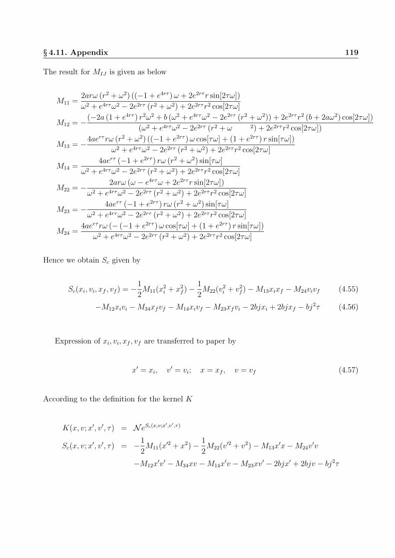
§ 4.11. Appendix 119
The result for MIJ is given as below
M11 =2arω (r2 + ω2) ((−1 + e4rτ )ω + 2e2rτr sin[2τω])
ω2 + e4rτω2 − 2e2rτ (r2 + ω2) + 2e2rτr2 cos[2τω]
M12 = −(−2a (1 + e4rτ ) r2ω2 + b (ω2 + e4rτω2 − 2e2rτ (r2 + ω2)) + 2e2rτr2 (b+ 2aω2) cos[2τω])
(ω2 + e4rτω2 − 2e2rτ (r2 + ω 2) + 2e2rτr2 cos[2τω])
M13 = −4aerτrω (r2 + ω2) ((−1 + e2rτ )ω cos[τω] + (1 + e2rτ ) r sin[τω])
ω2 + e4rτω2 − 2e2rτ (r2 + ω2) + 2e2rτr2 cos[2τω]
M14 =4aerτ (−1 + e2rτ ) rω (r2 + ω2) sin[τω]
ω2 + e4rτω2 − 2e2rτ (r2 + ω2) + 2e2rτr2 cos[2τω]
M22 = − 2arω (ω − e4rτω + 2e2rτr sin[2τω])
ω2 + e4rτω2 − 2e2rτ (r2 + ω2) + 2e2rτr2 cos[2τω]
M23 = − 4aerτ (−1 + e2rτ ) rω (r2 + ω2) sin[τω]
ω2 + e4rτω2 − 2e2rτ (r2 + ω2) + 2e2rτr2 cos[2τω]
M24 =4aerτrω (− (−1 + e2rτ )ω cos[τω] + (1 + e2rτ ) r sin[τω])
ω2 + e4rτω2 − 2e2rτ (r2 + ω2) + 2e2rτr2 cos[2τω]
Hence we obtain Sc given by
Sc(xi, vi, xf , vf ) = −1
2M11(x2
i + x2f )−
1
2M22(v2
i + v2f )−M13xixf −M24vivf (4.55)
−M12xivi −M34xfvf −M14xivf −M23xfvi − 2bjxi + 2bjxf − bj2τ (4.56)
Expression of xi, vi, xf , vf are transferred to paper by
x′ = xi, v′ = vi; x = xf , v = vf (4.57)
According to the definition for the kernel K
K(x, v;x′, v′, τ) = N eSc(x,v;x′,v′,τ)
Sc(x, v;x′, v′, τ) = −1
2M11(x′2 + x2)− 1
2M22(v′2 + v2)−M13x
′x−M24v′v
−M12x′v′ −M34xv −M14x
′v −M23xv′ − 2bjx′ + 2bjv − bj2τ

§ 4.11. Appendix 120
The conditional probability distribution is given by
P (x, v;x′, v′, τ) =eSc(x,v;x′,v′,τ)∫
dx′dv′eSc(x,v;x′,v′,τ)(4.58)
The marginal conditional probability distribution is given by
P (x, v;x′; τ) =
∫dv′P (x, v;x′, v′; τ)
=
√1
2πν2exp− 1
2ν2(−x′ + ζx+ ξv + j)
2 (4.59)
where
ν2 =2Ωrω[ω sinh(2rτ)− r sin(2ωτ)]
a (r2 + ω2)
ζ = 4Ωrω[(r2 − ω2
)sinh(rτ) sin(ωτ) + 2rω cosh(rτ) cos(ωτ)]
ξ = −4Ωrω[ω sinh(rτ) cos(ωτ) + r cosh(rτ) sin(ωτ)] (4.60)
and
Ω =1
(r2 + ω2)2 − r2 (r2 − 3ω2) cos(2ωτ)− ω2 (ω2 − 3r2) cosh(2rτ)(4.61)

Chapter 5
Risky Forward Interest Rates and
Swaptions: Quantum Finance Model
and Empirical Results
Both the US forward interest rates and the term structure for the spread are modeled by a two
dimensional Euclidean quantum field. As a precursor to the evaluation of put option of the
Singapore coupon bond, the quantum finance model for swaptions is tested using empirical
study of swaptions for the US Dollar – showing that the model is quite accurate. A prediction
for the market price of the put option for the Singapore coupon bonds is obtained. The
quantum finance model is generalized to study the Malaysian case and the Malaysian forward
interest rates are shown to have anomalies absent for the US and Singapore case. The model’s
prediction for a Malaysian interest rate swap is obtained.
§ 5.1 Introduction
Coupon and zero coupon bonds form the bedrock of the debt market [40, 41, 42]. Quantum
finance models of risk free coupon bonds match market data very well [1] and so it is natural
121

§ 5.1. Introduction 122
to extend the analysis to coupon bonds that carry issuer country’s risk of default. The
possibility of default results, as is well known, results in an issuer having to pay coupons on
risky bonds[43, 44] that are higher than the risk free case – the spread being determined by
rating agencies.
In Sections § 5.2, § 5.3 and § 5.4, the quantum finance model for the risk free and risky
forward interest rates are defined; the correlation functions of the model are evaluated and
an explicit expression for the stiff propagator is obtained. The market correlator is defined
in Section § 5.5, and the empirical calibration of all the parameters of the model, for the US,
Singapore and Malaysian forward interest rates are obtained and summarized in Sections § 5.6,
§ 5.8 and § 5.9. The swaption for the forward interest rates is defined in Section § 5.10 and the
US, Singapore and Malaysian markets are empirically analyzed. The results of the paper are
summarized in Section § 5.11.
Sections § 5.12 to § 5.16 are Appedicies to the main text. The derivation of the risky
coupon bond option is carried out in Section § 5.12, and in Section§ 5.13 the equations used
in the empirical analysis are derived from first principles. Swaption data in the market is
given in terms of Black’s swaption formula, and a derivation of this is given in Section § 5.14.
Section § 5.15 is a summary of the algorithm required to obtained the zero coupon bonds from
coupon bonds and Section § 5.16 derives an efficient algorithm to obtain an accurate result fo
the forward interest rates from the zero coupon bonds.
Although we did not use Sections § 5.15 and § 5.16 in our empirical analysis since we
obtained risk free and risky forward interest rates from Bloomberg, for many emerging mar-
kets forward interest rates data is not available and only the sovereign coupon bond data is
available; for these cases one needs the results of Sections § 5.15 and § 5.16 to carry out the
analysis.

§ 5.2. Quantum finance model of forward interest rates 123
§ 5.2 Quantum finance model of forward interest rates
The risk free US zero coupon bonds B(t, T ) are determined by the forward interest rates
f(t, x) as follows
B(t, T ) = exp−∫ T
t
dxf(t, x).
As shown in Figure 5.1(a), let calendar time t be the vertical axis, and let the horizontal
axis x > t be future time. The shaded portion represents the forward interest rates f(t, x):
every point in the shaded domain corresponds to one forward interest rate.
t0
t0Future Time x
Cal
endar
Tim
e t
x = t
f(t0, x)
0T
0t
0T iT
Future Time
Cal
endar
Tim
e
0t
B ( , )0T iT
B ( , )0t iT
Figure 5.1: a) The semi-infinite domain with two boundaries on which f(t, x) and A(t, x) aredefined. b) The zero coupon bond for two different times t0 and T0.
The zero coupon bonds B(t, T ) is shown in Figure 5.1(b) at two different calendar time t0
and T0 . The shaded domain shows the forward interest rates that are bounded by the two
coupon bonds.
In the quantum finance formulation of forward interest rates, the two-dimensional Eu-
clidean quantum field A(t, x) is a random stochastic field driving the forward interest rates;
the forward rates f(t, x) are given by [1]
∂f
∂t(t, x) = α(t, x) + σ(t, x)A(t, x) (5.1)
⇒ f(t, x) = f(t0, x) +
∫ t
t0
dt′α(t′, x) +
∫ t
t0
dt′σ(t′, x)A(t′, x). (5.2)
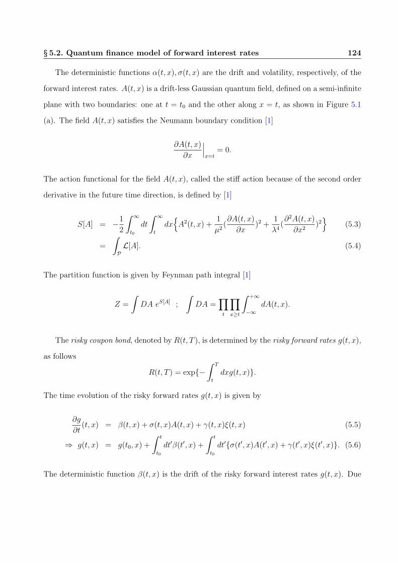
§ 5.2. Quantum finance model of forward interest rates 124
The deterministic functions α(t, x), σ(t, x) are the drift and volatility, respectively, of the
forward interest rates. A(t, x) is a drift-less Gaussian quantum field, defined on a semi-infinite
plane with two boundaries: one at t = t0 and the other along x = t, as shown in Figure 5.1
(a). The field A(t, x) satisfies the Neumann boundary condition [1]
∂A(t, x)
∂x
∣∣∣x=t
= 0.
The action functional for the field A(t, x), called the stiff action because of the second order
derivative in the future time direction, is defined by [1]
S[A] = −1
2
∫ ∞t0
dt
∫ ∞t
dxA2(t, x) +
1
µ2(∂A(t, x)
∂x)2 +
1
λ4(∂2A(t, x)
∂x2)2
(5.3)
=
∫PL[A]. (5.4)
The partition function is given by Feynman path integral [1]
Z =
∫DA eS[A] ;
∫DA =
∏t
∏x≥t
∫ +∞
−∞dA(t, x).
The risky coupon bond, denoted by R(t, T ), is determined by the risky forward rates g(t, x),
as follows
R(t, T ) = exp−∫ T
t
dxg(t, x).
The time evolution of the risky forward rates g(t, x) is given by
∂g
∂t(t, x) = β(t, x) + σ(t, x)A(t, x) + γ(t, x)ξ(t, x) (5.5)
⇒ g(t, x) = g(t0, x) +
∫ t
t0
dt′β(t′, x) +
∫ t
t0
dt′σ(t′, x)A(t′, x) + γ(t′, x)ξ(t′, x). (5.6)
The deterministic function β(t, x) is the drift of the risky forward interest rates g(t, x). Due

§ 5.2. Quantum finance model of forward interest rates 125
to the trapezoidal structure of the domain of the forward interest rates, one can consistently
choose
α(t, x) = α(θ) ; β(t, x) = β(θ) ; σ(t, x) = σ(θ) ; γ(t, x) = γ(θ)
, where remaining future time θ is defined by
θ = x− t ≥ 0.
The basic assumption of our model is that the risky forward interest rates are driven by
the risk free forward interest rates f(t, x) – with the risky rates having a spread above the
risk free rates. The spread is given by the quantum field for the spread term structure, and is
denoted by ξ(t, x). The volatility of the spread is given by the deterministic function γ(t, x)
and is determined by its correlation function.
The spread also obeys the Neumann boundary condition
∂ξ(t, x)
∂x
∣∣∣x=t
= 0.
The stiff action functional for the risky forward interest rates is obtained by extending the
risk free case given in Eq. (5.3), and yields
S[A; ξ] = −1
2
∫ ∞t0
dt
∫ ∞t
dxA2(t, x) +
1
µ2(∂A(t, x)
∂x)2 +
1
λ4(∂2A(t, x)
∂x2)2
− 1
2
∫ ∞t0
dt
∫ ∞t
dxξ2(t, x) +
1
µ2(∂ξ(t, x)
∂x)2 +
1
λ2(∂2ξ(t, x)
∂x2)2
+
∫ ∞t0
dt
∫ ∞t
dxdx′∆(x− t, x′ − t)A(t, x)ξ(t, x′) (5.7)
=
∫PL[A; ξ].
The cross-term ∆(x− t, x′ − t) connects the fields A(t, z), ξ(t, z′) at the same calendar time,

§ 5.3. Correlation functions 126
but for different future times: this is consistent with the other terms in the Lagrangian, for
which all the terms are defined for the same calendar time.
The partition function is given by Feynman path integral
Z =
∫DADξ eS[A;ξ]. (5.8)
§ 5.3 Correlation functions
The auto- and cross-correlation functions of the risky and risk free interest rates can be
computed from the correlation functions of the quantum fields A(t, x), ξ(t, x). Using the
Neumann condition for the fields A(t, x), ξ(t, x), the action given in Eq. (5.7) yields, after an
integration by parts and in matrix notation, the following
S[A; ξ] = −1
2
∫ ∞t0
dt
∫ ∞t
dxdx′
[A(t, x) ξ(t, x)
]
×
(1− 1
µ2∂2
∂x2+ 1
λ4∂∂x4
)δ(x− x′) −∆(x− t, x′ − t)
−∆T (x− t, x′ − t) (1− 1µ2
∂2
∂x2+ 1
λ4∂∂x4
)δ(x− x′)
A(t, x′)
ξ(t, x′)
≡ −1
2
∫ ∞t0
dt
∫ ∞t
dxdx′
[A(t, x) ξ(t, x)
]M−1(x− t, x′ − t)
A(t, x′
ξ(t, x′)
(5.9)
where
M−1(x− t, x′ − t) =
D−1(x− t, x′ − t) −∆(x− t, x′ − t)
−∆T (x− t, x′ − t) C−1(x− t, x′ − t)
(5.10)

§ 5.3. Correlation functions 127
The risk free forward interest rates f(t, x) should be weakly correlated with the risky
forward interest rates g(t, x) since one does not expect, for instance, the Singapore bonds to
strongly influence the US zero coupon bonds. Hence, we expect that
|∆(x− t, x′ − t)| ≤ 0.1 ∀ x− t, x′ − t
An empirical analysis, discussed later in Section § 5.8, will approximately confirm this expec-
tation. All the calculations are done to O(∆).
Let
θ = x− t ; θ′ = x′ − t
To leading order in ∆, we have, in matrix notation
M(θ, θ′) ≡
M11(θ, θ′) M12(θ, θ′)
M21(θ, θ′) M22(θ, θ′)
=
D(θ, θ′) (D∆C)(θ, θ′)
(C∆TD)(θ, θ′) C(θ, θ′)
+O(∆2)(5.11)
The correlation function between the field’s fluctuations at two different future times is
given by the
E[A(t, x)A(t′, x′)] =1
Z
∫DADξ A(t, x)A(t′, x′)eS[A;ξ]
= M11(θ, θ′) = δ(t− t′)D(θ, θ′) +O(∆2). (5.12)
where the δ(t− t′) has been factored out for future convenience. The correlation function of
the spread is determined by
E[ξ(t, x)ξ(t′, x′)] =1
Z
∫DADξ ξ(t, x)ξ(t′, x′)eS[A;ξ]
= M22(θ, θ′) = δ(t− t′)C(θ, θ′) +O(∆2). (5.13)

§ 5.3. Correlation functions 128
For the action given in Eq. (5.7), it follows that
1− 1
µ2
∂2
∂x2+
1
λ4
∂4
∂x4
D(θ, θ′)
∣∣∣Neumann
= δ(x− x′) +O(∆2), (5.14)
and
1− 1
µ2
∂2
∂x2+
1
λ4
∂4
∂x4
C(θ, θ′)
∣∣∣Neumann
= δ(x− x′) +O(∆2). (5.15)
D(θ, θ′), C(θ, θ′) are propagators that measure the effect that the fluctuations of the fields
A(t, θ+ t), ξ(t, θ+ t) at point t, x has on the fluctuations of A(t′, θ′+ t), ξ(t′, θ′+ t′) at another
point t′, x′, respectively.
The cross-correlation function of the risk free forward rates f(t, x) with the spread ξ(t, x)
is given by
E[A(t, x)ξ(t′, x′)] =1
Z
∫DADξ A(t, x)ξ(t′, x′)eS[A;ξ]
= M12(θ, θ′) = δ(t− t′)(D∆C)(θ, θ′) +O(∆2). (5.16)
Note that the result above for E[A(t, x)ξ(t′, x′)] is not a symmetric matrix since the two fields
are in-equivalent.
The concept of market time is required for relating the action functional to the empirical
correlation functions. The Lagrangian is written in terms of market future time z given by
x→ z = ω
(x− tω
)η: x ∈ [t,∞] ⇒ z ∈ [0,∞]

§ 5.4. Stiff propagator 129
The action functional describing the market’s behavior is given by [1]
S[A; ξ] = −1
2
∫ ∞t0
dt
∫ ∞0
dzA2(t, z) +
1
µ2(∂A(t, z)
∂z)2 +
1
λ4(∂2A(t, z)
∂z2)2
− 1
2
∫ ∞t0
dt
∫ ∞0
dzξ2(t, z) +
1
µ2(∂ξ(t, z)
∂z)2 +
1
λ4(∂2ξ(t, x)
∂z2)2
+
∫ ∞t0
dt
∫ ∞0
dzdz′∆(z, z′)A(t, z)ξ(t, z′) (5.17)
=
∫PL[A; ξ].
§ 5.4 Stiff propagator
The Neumann boundary condition leads to the following Fourier expansion
A(t, x) =
∫ +∞
0
dk
π/2eiωt cos(kθ)A(t, k) ; θ = x− t (5.18)
The stiff propagator is given by [1]
D(θ; θ′) = λ4
∫ +∞
0
dk
π/2
cos(k(x− t)) cos(k(x′ − t))λ4 + λ4
µ2k2 + k4
= λ4
∫ +∞
−∞
dk
2π· e
ik(x+x′−2t) + eik(x−x′)
λ4 + λ4
µ2k2 + k4
(5.19)
Note that
λ4 + (λ2/µ)2k2 + k4 = (k2 + α+)(k2 + α−)
with α± =λ4
2µ2[1±
√1− 4(
µ
λ)4 ]

§ 5.4. Stiff propagator 130
and yields
1
λ4 + (λ2/µ)2k2 + k4=( 1
α+ − α−)[
1
k2 + α−− 1
k2 + α+
] (5.20)
Define new variables
θ± = θ ± θ′ where θ = x− t ; θ′ = x′ − t (5.21)
Eqs. (5.19) and (5.20) yield
D(θ+; θ−) =( λ4
α+ − α−)[ 1
α−d(θ+; θ−;
√α−)− 1
α+
d(θ+; θ−;√α+)
](5.22)
where
d(θ+; θ−;√α±) =
√α±
2
[e−√α±θ+ + e−
√α±|θ−|
](5.23)
The solution for α± yields three distinct cases, namely, when α± is real, complex or
degenerate, each with unique characteristics [3]. From the previous studies of quantum finance
models of interest rates, the real branch of the stiff propagator is realized in the debt market
[1], for which
µ <√
2λ ⇒ α± : Real
Choose the following parametrization
α± = λ2e±b ; e±b =λ2
2µ2
[1±√
1− 4(µ
λ)4]
; b ≥ 0 (5.24)

§ 5.5. Market correlators 131
Note the system is critical for λ2 = 2µ2 ⇒ b = 0, and yields
α+ = α−
In this parametrization, from Eqs.(5.22) and (5.23)
Gb(θ+; θ−) =λ
2 sinh(2b)
[e−λθ+ cosh(b) sinhb+ λθ+ sinh(b)+
e−λ|θ−| cosh(b) sinhb+ λ|θ−| sinh(b)]
(5.25)
§ 5.5 Market correlators
Both calendar and future time are discretized; for ease of notation, only calendar time is
explicitly discretized and future time is written in the continuum notation. Hence
f(t, x) = f(t, θ + t)→ f(tn, θ + tn) ; g(t, x)→ g(tn, θ + tn) ; tn = εn ; θ = x− tn.
Time derivative is approximated by a finite difference and
∂f(t, x)
∂t→ 1
ε(f(tn, θ + tn)− f(tn−1, θ + tn−1)) ≡ 1
εδf(tn, θ + tn)
similarly
∂g(t, x)
∂t→ 1
εδg(tn, θ + tn)
The evolution equation yields
δf(tn, θ + tn) = εα(tn, θ + tn) + εσA(tn, θ + tn), (5.26)
δg(tn, θ + tn) = εβ(tn, θ + tn) + εσA(tn, θ + tn) + εγξ(tn, θ + tn). (5.27)

§ 5.5. Market correlators 132
All correlation functions depend only on remaining time θ = x − t; this property of the
quantum field theory model is crucial in the empirical analysis.For any correlation function
O(t, x; t′x′), one has for the expectation value
E[O(t, x; t′, x′)] = E[O (t, t+ (x− t); t′, t′ + (x′ − t′))] = δ(t− t′)Φ(θ, θ′).
Setting t = t′, and using the fact that for discretized time, we have
δ(0) =1
ε
yields
E[O(t, x; t, x′)] = E[O (t, θ + t; t, θ′ + t)] =1
εΦ(θ, θ′). (5.28)
Correlation functions are evaluated by assuming averages over historical data are equal to
ensemble averaging. Hence, due to Eq. (5.28), holding θ, θ′ fixed, a sum is taken over the past
historical data to yield
Φ(θ, θ′) = εE[O(t, x; t, x′)] ≡ ε
N
n=−1∑−N
O (tn; tn + θ; tn + θ′) .
Define the connected correlator by
E[AB]c = E[AB]− E[A]E[B].

§ 5.5. Market correlators 133
The connected correlation functions, for t = t′, from Eqs. (5.12) and (5.16) and using δ(0) =
1/ε, are given by
E[δf(t, x)δf(t′, x′)]c = δ(t− t′)ε2σ(θ)DE(θ, θ′)σ(θ′) = εσ(θ)DE(θ, θ′)σ(θ′) (5.29)
E[δ(g − f)(t, x)δ(g − f)(t′, x′)]c = δ(t− t′)ε2γ(θ)CE(θ, θ′)γ(θ′) = εγ(θ)CE(θ, θ′)γ(θ′) (5.30)
For equal time t = t′, note that the definition of volatilities σ, γ in the defining equations Eq.
(5.1) and (5.5) can be changed up to a scaling factor, which is taken to be equal to 1/εD(θ, θ)
and 1/εC(θ, θ), respectively. Using this scale factor, one obtains [7]
εDE(θ, θ) = 1 = εCEθ, θ) (5.31)
To simplify the notation, for equal time one can ignore the time index since the correlator
does not depend on it. We adopt the notation
E[δf(t, t+ θ)δg(t, t+ θ′)] ≡ E[δfδg](θ, θ′) (5.32)
In this notation, the result given in Eqs. (5.29) and (5.30) is written as
E[δfδf ]c(θ, θ′) = σ(θ)DE(θ, θ′)σ(θ′) ; E[δ(g − f)δ(g − f)]c(θ, θ
′) = γ(θ)CE(θ, θ′)γ(θ′)
The normalization given in Eq. (5.31) yields, from Eqs. (5.29) and (5.30), that
E[(δf(t, x)
)2
]c = E[δfδf ]c(θ, θ) = σ2(θ) (5.33)
E[(δ(g − f)(t, x)
)2
]c = E[δ(g − f)δ(g − f)]c(θ, θ) = γ2(θ) (5.34)
The empirical propagators DE(θ, θ′), CE(θ, θ′) and volatilities σ, γ are evaluated from Eqs.

§ 5.5. Market correlators 134
(5.29), (5.30), (5.33) and (5.34). Note the important result that the volatilities σ, γ are not
model dependent but rather, are directly obtained from the market without any fitting. This
greatly increases the accuracy of the model and incorporates important market information
into the results of the model.
The models propagators D(z(θ), z(θ′)), C(z(θ), z(θ′)) provide a fit of the model’s param-
eter using the relation
DE(θ, θ′) = D(z(θ), z(θ′)) = D(z, z′) ; CE(θ, θ′) = C(z(θ), z(θ′)) = C(z, z′)
where recall market time is given by
z(θ) = ω
(θ
ω
)η; θ = x− t
The cross-correlator is fixed uniquely by Eqs. (5.33) and (5.34) and yields
E[δfδ(g − f)]c(θ, θ′) = σ(θ)(DE∆ECE)(θ, θ′)γ(θ′)
Define the empirical cross-correlator
TE(θ, θ′) ≡ E[δfδ(g − f)]c(θ, θ′)
σ(θ)γ(θ′)(5.35)
The empirical cross-correlator, in matrix notation, is given by
∆E(θ, θ′) =(D−1E TEC
−1E
)(θ, θ′) (5.36)
The model cross-correlator ∆(z(θ), z(θ′)) is given by the mapping from the empirical cross-

§ 5.6. Empirical volatility and propagators 135
correlator ∆E(θ, θ′) using the concept of market time z(θ). We hence obtain
∆(z(θ), z(θ′)) = ∆E(θ, θ′)
Defining
z−1(θ) = ω(θ
ω)1/η ⇒ ∆(θ, θ′) = ∆E(z−1(θ), z−1(θ′)) (5.37)
It is the coefficient function ∆(θ, θ′) that appears in Lagrangian, with θ, θ′ being replaced by
independent integration variables z, z′ in the action.
In summary, the calibration of the risky forward rates yields the following results.
• Parameters µ, λ, µ, λ and ω, η.
• Functions σ(θ), γ(θ).
• Function ∆(z, z′).
§ 5.6 Empirical volatility and propagators
0
0.5
1
1.5
2
2.5
3
3.5
4x 10
−6
0 1 2 3 4 5 6 7 8 9 10
Time to maturity(year)
σ2(θ
) (\
ye
ar)
0
0.5
1
1.5
2
2.5
3
3.5
4
4.5x 10
−6
0 1 2 3 4 5 6 7 8 9 10
Time to maturity(year)
σ2(θ
) (\
ye
ar)
Figure 5.2: (a) Volatility of US forward interest rates. (b) Volatility of the spread of theSingapore -US forward interest rates. Period from 9 May 2011 to 18 January, 2012.

§ 5.6. Empirical volatility and propagators 136
All the data for the US, Singapore and Malaysian forward interest rates is daily data taken
from Bloomberg, for the period from 9 May 2011 to 18 January, 2012.
The volatility of the US forward interest rates f(t, x) and of the Singapore spread ξ(t, x) =
g(t, x)−f(t, x) is determined from market data using Eqs. (5.33) and (5.34) respectively, and
shown in Figure 5.2. Both the volatilities are of the same order of magnitude. The volatility
of the spread ξ(t, x) follows the US case, as is to be expected since the US debt market drives
the international debt market.
Compared to earlier period of 1999-2001, there has been a dramatic change in the volatility
of the US forward interest rates since – or more likely due to – the 2008 financial meltdown,
and shown in Figure 5.3. The volatility for 2011-2012 is seen, in Figure 5.2, to increase
indefinitely as one goes to future time, as opposed to the volatility for the 1999-2001 period,
which has a maximum for future time of about 1.5 years in the future around 2001-2 and then
leveling off as one goes indefinitely into the future.
Figure 5.3: Empirical volatility function σ(θ) =√E[δf 2(t, θ)]c and kurtosis κ(t, θ) =
E[δf(t, θ)4]/σ4(t, θ)− 3 of the forward interest rates; θ = x− t. (Reference: [1]).
One can interpret the change of behavior of the US forward interest rates from 2000 to
2011 as implying that, unlike during the pre-2008 period, the volatility – and hence the risk
of the debt market – since 2008 has been increasing indefinitely for future time pointing to a
future that is increasingly unstable.

§ 5.6. Empirical volatility and propagators 137
The test of the model is to compare the model’s correlators of the forward rates for the
risk free and risky case, given by D(z(θ), z(θ′)), C(z(θ), z(θ′)), with the empirical correlators
DE(θ, θ′), CE(θ, θ′). The calibration is done via the equation
D(z, z′) = D(z(θ), z(θ′)) = DE(θ, θ′) =E[δfδf ]c(θ, θ
′)
σ(θ)σ(θ′)
and
C(z, z′) = C(z(θ), z(θ′)) = CE(θ, θ′) =E[δ(g − f)δ(g − f)]c(θ, θ
′)
γ(θ)γ(θ′)
One of the major advantages of the model is that the functions σ(θ), γ(θ) and ∆(z, z′) can be
directly obtained from the empirical correlator without the need to do any fits. This feature
greatly increases the accuracy of the model.
§ 5.6.1 Stand-alone Singapore rates
Consider a stand-alone model for the Singapore forward rates g(t, x), similar to the risk free
case as in Eq. (5.1) and given by
∂g
∂t(t, x) = d(t, x) + s(t, x)B(t, x) (5.38)
and the Euclidean quantum field B(t, x) has an action similar to A(t, x). The stand-alone
empirical volatility is given by
s2(t, x) = E[(δg)2]c
Note that
E[(δ(g − f))2]c = E[(δg)2]c + E[(δf))2]c − 2E[δgδf)]c (5.39)

§ 5.7. Calibration of US and Singapore models 138
This yields
γ2 = s2 + σ2 − 2E[δgδf)]c (5.40)
Eq. (5.40) is shown in Figure 5.4, and the volatilities are consistent.
0
0.2
0.4
0.6
0.8
1
1.2x 10
−6
0 1 2 3 4 5 6 7 8 9 10
Time to maturity(year)
σ2(θ
) (\
ye
ar)
0
0.5
1
1.5
2
2.5
3
3.5
4
4.5x 10
−6
γ2
s2+σ
2−2E[dgdf]
0 1 2 3 4 5 6 7 8 9 10
σ2(θ
) (\
ye
ar)
Time to maturity(year)
Figure 5.4: (a) Volatility of the Singapore stand-alone forward interest rates. (b) Comparisonof volatility of Singapore stand-alone forward interest rates of the US and spread of theSingapore -US forward interest rates. Period from 9 May 2011 to 18 January, 2012.
The model’s propagator is given by
C(z(θ), z(θ′)) = CE(θ, θ′) =E[δgδg]c(θ, θ
′)
s(θ)s(θ′)
A fit of the model’s parameters with the empirical result is carried out to ascertain the accuracy
of the stand-alone simplified model.
§ 5.7 Calibration of US and Singapore models
The models of the forward interest rates for the US and Singapore are calibrated using the
empirical correlators. The empirical value and the best fit of the model is evaluated for the

§ 5.7. Calibration of US and Singapore models 139
0
5
10
15
0
2
4
6
8
10
12
14−0.2
0
0.2
0.4
0.6
0.8
1
1.2
0
2
4
6
8
10
12
0
2
4
6
8
10
12
0
0.2
0.4
0.6
0.8
1
Figure 5.5: US forward interest rates. (a) The empirical correlator DE(θ, θ′). (b) The modelcorrelator D(θ, θ′). Data from 9 May 2011 to 18 January, 2012.
0
2
4
6
8
10
12
0
2
4
6
8
10
12
0.5
0.6
0.7
0.8
0.9
1
0
2
4
6
8
10
12
0
2
4
6
810
12
0.4
0.5
0.6
0.7
0.8
0.9
1
Figure 5.6: Singapore forward interest rates. (a) The empirical correlator CE(θ, θ′). (b) Themodel correlator C(θ, θ′). Data from 9 May 2011 to 18 January, 2012.
US forward interest rates as follows
DE(θ, θ′) =E[δfδf ]c(θ, θ
′)
σ(θ)σ(θ′)= D(z(θ), z(θ′))
The results are shown in Figure 5.5. For the stand alone Singapore forward interest rates
CE(θ, θ′) =E[δgδg]c(θ, θ
′)
s(θ)s(θ′)= C(z(θ), z(θ′))
and the results are shown in Figure 5.6.

§ 5.8. Determination of ∆(θ, θ′): Coupling of US-Singapore rates 140
The empirical correlator for the spread of the Singapore forward interest rates above the
US forward interest rates is given by
C(z, z′) = CE(θ, θ′) =E[δ(g − f)δ(g − f)]c(θ, θ
′)
γ(θ)γ(θ′)= C(z(θ), z(θ′))
The results of calibrating the propagators is given in Table 5.1.
02
46
810
12
0
2
4
6
8
10
12
−0.2
0
0.2
0.4
0.6
0.8
1
1.2
0
2
4
6
8
10
12
0
2
4
6
8
10
12
0
0.2
0.4
0.6
0.8
1
Figure 5.7: Joint US-Singapore forward curve. (a) The empirical spread correlator CE(θ, θ′).(b) The model spread correlator C(θ, θ′). Data from 9 May 2011 to 18 January, 2012.
Note that the unit of the axis in the 3D graphs from Section 8 to Section 9 are for the
payment period, which is half a year in this chapter.
§ 5.8 Determination of ∆(θ, θ′): Coupling of US-Singapore
rates
The empirical cross-correlator, from Eq. (5.36) and in matrix notation, is given by
∆E(θ, θ′) =(D−1E TC−1
E
)(θ, θ′)

§ 5.8. Determination of ∆(θ, θ′): Coupling of US-Singapore rates 141
Note that all the matrices on the right hand side of above equation are empirically determined.
The value of ∆E(θ, θ′) evaluated from above equation has large errors. The reason is that on
numerically inverting DE and CE, both D−1E and C−1
E have large errors, of order 107. This is
due to the fact that both are differential operator, and which are approximately given by the
model’s values as in Eqs. (5.14) and (5.15).
0
5
10
1520
0
5
10
15
20
−0.2
0
0.2
0.4
0.6
0.8
1
1.2
0
5
10
15
20
0
5
10
15
20
−0.4
−0.2
0
0.2
0.4
0.6
0.8
1
1.2
0
5
10
15
20
0
5
10
15
20
0
0.2
0.4
0.6
0.8
1
Figure 5.8: Inverse of propagator: (a) D−1DE (b) C−1CE (c) The Dirac delta function δ(θ−θ′).Data from 9 May 2011 to 18 January, 2012.
Hence, instead of inverting the empirical propagators DE and CE, the empirical inverses
are replaced by the model’s value for their inverses D−1, C−1 given by Eqs. (5.14) and (5.15);
more precisely
(D−1DE)(θ, θ′) =
(1− 1
µ2D
∂2
∂θ2+
1
λ4D
∂4
∂θ4
)DE(θ, θ′) = δ(θ − θ′)
and
(C−1CE)(θ, θ′) =
(1− 1
µ2c
∂2
∂θ′2+
1
λ4c
∂4
∂θ′4
)CE(θ, θ′) = δ(θ − θ′)
Figure 5.8(a) and (b) shows that the model’s values for the inverse of DE and CE is fairly
accurate, with the off-diagonal elements all falling to small values. Comparing Figure 5.8 with
the numerical representation of the Dirac δ−function, given in Figure 5.8(c), shows that there
are significant errors. Approximating D−1E and C−1
E by the models values given by D−1, C−1
introduce errors that are far smaller than inverting DE and CE.

§ 5.8. Determination of ∆(θ, θ′): Coupling of US-Singapore rates 142
The model’s inverse of the propagator yields the empirical cross-correlator, which in matrix
notation is given by
∆E(θ, θ′) =(D−1TEC
−1)
(θ, θ′)
Rrecall the matrix TE(θ, θ′) is empirically evaluated by
TE(θ, θ′) ≡ E[δfδ(g − f)]c(θ, θ′)
σ(θ)γ(θ′)
Hence, one obtains the following final result for ∆E(θ, θ′)
∆E(θ, θ′) =
(1− 1
µ2D
∂2
∂θ2+
1
λ4D
∂4
∂θ4
)(1− 1
µ2c
∂2
∂θ′2+
1
λ4c
∂4
∂θ′4
)TE(θ, θ′) (5.41)
The computation of ∆E(θ, θ′) requires, as can be seen from Eq. (5.41), both the empirical
value of the cross-correlator TE as well as the inverse of model’s propagators. The empirical
result for TE is shown in Figure 5.9(c) and ∆E(θ, θ′) is shown in Figure 5.9(b). The coefficient
function, from Eq. (5.37), is given by
∆(θ, θ′) = ∆E(z−1(θ), z−1(θ′))
and is shown in Figure 5.9(c).
0
5
10
15
20
0
5
10
15
20−1
−0.8
−0.6
−0.4
−0.2
0
0.2
0.4
05
1015
20
05
1015
20−1.4
−1.2
−1
−0.8
−0.6
−0.4
−0.2
0
0.2
0.4
0.6
0
2
4
6
8
10
0
2
4
6
8
10−1.2
−1
−0.8
−0.6
−0.4
−0.2
0
0.2
0.4
0.6
Figure 5.9: Correlation of Singapore - US forward interest rates spread with the US forwardinterest rates. (a) The cross-correlator TE. (b) ∆E of the US forward interest rates with thespread with the Singapore forward interest rates. (c) The model coefficient function ∆. Datafrom 9 May 2011 to 18 January, 2012.

§ 5.8. Determination of ∆(θ, θ′): Coupling of US-Singapore rates 143
The diagonal value of ∆(θ, θ) is near the value of 1, with the off-diagonal values of ∆(θ, θ′)
being less than 0.4. We can tentatively conclude that our assumption of the US and Singapore
forward interest rates being weakly coupled is approximately correct. The fact that ∆(θ, θ) ' 1
can be due to the fact that the spread ξ(t, z) is most strongly correlated with A(t, z) for equal
future time.
§ 5.8.1 Malaysian forward interest rates
The Malaysian forward interest rates h(t, x) are irregular, with features that are absent for
both the US and Singapore cases. The model for the Malaysian forward interest rates and its
spread over the US is defined by the following
∂h
∂t(t, x) = m(t, x) + v(t, x)M(t, x) (5.42)
∂(h− f)
∂t(t, x) = n(t, x) + ζ(t, x)(M − A)(t, x) (5.43)
The Euclidean quantum field M(t, x) and the spread M(t, x) − A(t, x) has an action similar
to A(t, x).
The volatility function, defined similar to the US and Singapore case, is given by
E[(δh(t, θ))2]c = v2(θ) ; θ = x− t
The empirical volatility of the Malaysian forward interest rates, v2(θ), is shown in Figure 5.10.
A noteworthy feature is that unlike the US forward interest rates, volatility v2(θ) plateaus
after 9 years.

§ 5.8. Determination of ∆(θ, θ′): Coupling of US-Singapore rates 144
2
4
6
8
10
12
14x 10
−4
0 1 2 3 4 5 6 7 8 9 10
Time to maturity(year)
σ(θ
) (\
ye
ar)
2
4
6
8
10
12
14
16x 10
−4
Time to maturity(year)
σ(θ
) (\
ye
ar)
0 1 2 3 4 5 6 7 8 9 10
Figure 5.10: (a) The Malaysian forward interest rates volatility v2(θ); half-yearly time steps inthe future time direction. (b) The volatility ζ(θ) of the Malaysian spread over the US forwardinterest rates. Data from 9 May 2011 to 18 January, 2012.
The propagator is given by the normalized correlation function (θ = x− t; θ′ = x′ − t)
H(θ, θ′) =E[δh(t, θ)δh(t, θ′)]
v(θ)v(θ′); H(θ, θ′) =
E[δ(h− f)(t, θ)δ(h− f)(t, θ′)]
ζ(θ)ζ(θ′)
The propagator H(θ, θ′) has values that are negative for future times such that |θ − θ′| >
1.5 years, as shown in Figure 5.11(a). This implies that the forward interest rates 1.5 years
in the future move in the opposite direction to present day rates. Negative correlations
are almost absent in both the US (only a few points are slightly negative) and Singapore
correlation functions. It needs to be studied if there are any regulations on the Malaysian
debt market that is responsible for this behavior.
0
5
10
15
20
0
5
10
15
20
−0.6
−0.4
−0.2
0
0.2
0.4
0.6
0.8
1
1.2
0
5
10
15
20
0
5
10
15
20
−0.6
−0.4
−0.2
0
0.2
0.4
0.6
0.8
1
1.2
0
5
10
15
20
0
5
10
15
20
0
0.2
0.4
0.6
0.8
1
Figure 5.11: (a) The Malaysian stand-alone propagator H(θ, θ′). (b) Propagator for thespread, given by H(θ, θ′), of the Malaysian above the US forward interest rates. (c) Themodel fitting the spread for Malaysian forward interest rates. Data from 9 May 2011 to 18January, 2012.

§ 5.9. Summary of Calibration Results 145
If one studies the spread of the Malaysian forward interest rates above the US, given by
h(t, x) − f(t, x), one obtains the result given in Figure 5.11(b); the negative correlation is
alleviated a bit.
The model generates only positive values propagators, as can be seen from the fit of the
US and Singapore forward interest rates. The spread for the Malaysian can be fit by the
model , but with large errors, and the result is shown in Figure 5.11(c). The R2 = 0.58 for
the Malaysian spread is not a very good fit, primarily because of the negative values of the
empirical propagator.
§ 5.9 Summary of Calibration Results
Recall, from Eq. (5.24), the following are the parameters of the action
α± = λ2e±b ; e±b =λ2
2µ2
[1±√
1− 4(µ
λ)4]
; b ≥ 0
The calibration of the US, Singapore and Malaysian forward interest rates yields the results
given in Table 5.1.
The calibration for the forward interest rates has a number of key features. Firstly, the
accuracy of the calibration of the US and Singapore stand-alone model is comparable, with
R2 equal to 0.79 and 0.74 respectively. Secondly, modeling the Singapore forward interest
rates as being driven by the US rates is marginally more accurate, yielding a R2 equal to 0.80.
Lastly, the value of market time, given by η, ω, for the two cases for the Singapore forward
interest rates is quite different from the US.
Different model’s propagators R2 λ b η ω µ
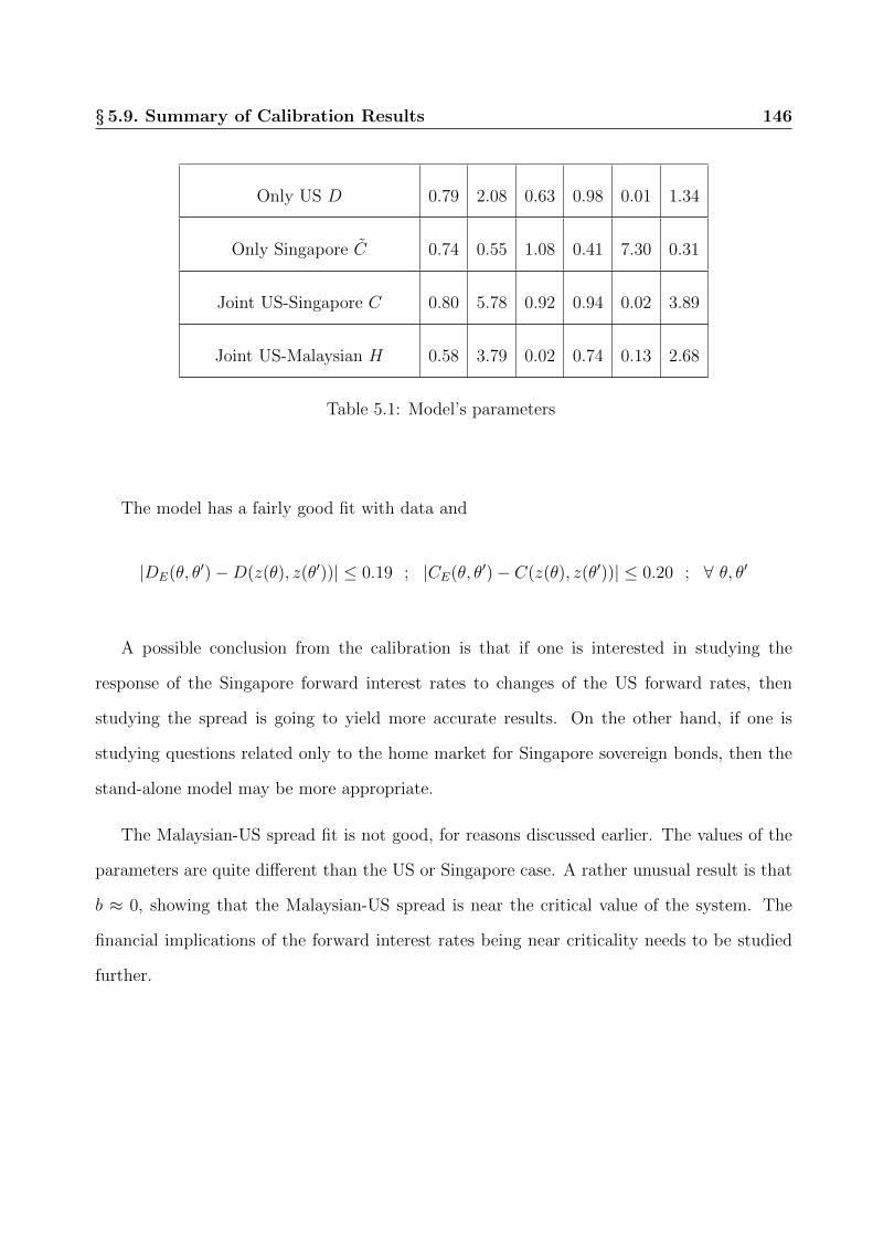
§ 5.9. Summary of Calibration Results 146
Only US D 0.79 2.08 0.63 0.98 0.01 1.34
Only Singapore C 0.74 0.55 1.08 0.41 7.30 0.31
Joint US-Singapore C 0.80 5.78 0.92 0.94 0.02 3.89
Joint US-Malaysian H 0.58 3.79 0.02 0.74 0.13 2.68
Table 5.1: Model’s parameters
The model has a fairly good fit with data and
|DE(θ, θ′)−D(z(θ), z(θ′))| ≤ 0.19 ; |CE(θ, θ′)− C(z(θ), z(θ′))| ≤ 0.20 ; ∀ θ, θ′
A possible conclusion from the calibration is that if one is interested in studying the
response of the Singapore forward interest rates to changes of the US forward rates, then
studying the spread is going to yield more accurate results. On the other hand, if one is
studying questions related only to the home market for Singapore sovereign bonds, then the
stand-alone model may be more appropriate.
The Malaysian-US spread fit is not good, for reasons discussed earlier. The values of the
parameters are quite different than the US or Singapore case. A rather unusual result is that
b ≈ 0, showing that the Malaysian-US spread is near the critical value of the system. The
financial implications of the forward interest rates being near criticality needs to be studied
further.

§ 5.10. Interest rate swaptions 147
§ 5.10 Interest rate swaptions
Interest rate swaps for US$ are widely traded instruments. The empirical study of swaptions
– options on swaps – can be used for testing and calibrating the quantum finance models for
coupon bond options.
There are swaptions traded in the market in which the floating rate is paid at ` = 90 days
intervals, and the fixed rate payments are paid at 2` = 180 days intervals. For a swaption
with fixed rate payments at 90 days intervals – at times T0 +n`, with n = 1, 2.., N – there are
N payments. For payments made at 180 days intervals, there are only N/2 payments 1 made
at times T0 + 2n` , n = 1, 2, ..., N/2, and of amount 2RS.
Define the following positive valued function
[A]+ =
A : A ≥ 0
0 : A < 0
The payoff function for a swaption is2
CL(t, T0;RS) = V[B(t, T0)−B(T0, T0 +N`)− 2`RS
N/2∑n=1
B(t, T0 + 2n`)]
+
= V[B(t, T0)−
N/2∑n=1
cnB(t, T0 + 2n`)]
+. (5.44)
The equivalent coupon bond put option, maturing at time t∗ and with payoff function is
1Suppose the swaption has a duration such that N is even. Note that for N = 4 the underlying swap hasa duration of one year.
2The price of CR for the case of 90 days floating and 180 days fixed interest payments is given from CL byusing the put-call relation similar to the one given in [1].
§ 5.10. Interest rate swaptions 148
given by
(K −
N/2∑n=1
cnB(t∗, T0 + 2n`))
+. (5.45)
and has the coefficients ci and strike price given by
cn = 2lRs; n = 1, 2....(N − 1)/2 : semi− annual payments at T0 + 2n`
cn/2 = 1 + 2lRs; : annual payments at T0 + n`
K = B(t, T0)
For the US Dollar swaption, let
Ji = ciFi ; F = exp−∫ Ti
t∗dxf(t0, x) ; F =
∑i
Ji
where f(t, x) is the risk free US Dollar forward yield curve; f(t0, x) is the yield curve at time
t0 and is taken from the market. The value of the risk free swaption – receiving floating Libor
and paying fixed interest rate – in the quantum finance model is given by [1]
C(t0, t∗, K) = B(t0, t∗)
√C2
2π− 1
2B(t0, t∗)(K − F ) +O(X2) (5.46)
The put swaption – for receiving fixed interest rate and paying the floating Libor rate – is
given by put-call parity and yields [1]
P (t0, t∗, K) = B(t0, t∗)
√C2
2π+
1
2B(t0, t∗)(K − F ) +O(X2) (5.47)

§ 5.10. Interest rate swaptions 149
From Eq. (5.81)
C2 =N∑ij=1
JiJj[eGij − 1] '
N∑ij=1
JiJjGij +O(σ2γ2, σγ3, σ3γ) (5.48)
Ti--t
0
Ti-t
0t*-t
0
t*-t
0
‘Tj-t
0
Ti-t
0t*-t
0
t*-t
0
‘
0 0
(a) (b)
Figure 5.12: Domain for Gij. (a) For the case of Ti = Tj. (b) For the case of Ti 6= Tj.
The integrations for Gij are written in terms of future time θ = x− t, θ′ = x′ − t as this
is required for the empirical analysis. Hence
Gij =
∫ t∗
t0
dt
∫ Ti
t∗
dx
∫ Tj
t∗
dx′σ(x− t)D(x− t, x′ − t)σ(x′ − t)
=
∫ t∗
t0
dt
∫ Ti−t
t∗−tdθ
∫ Tj−t
t∗−tdθ′E[δfδf ]c(θ, θ
′) (5.49)
The quantum finance model for the forward interest rates yield the expression for the option
price C(t0, t∗, K) in terms of the correlators E[δfδf ]c(θ, θ′). The correlator in turn is taken
directly from the market data.
Note that the integrand of Gij in Eq. (5.49) is over future calendar time – from t0 to t∗.
However, using the fact that the correlators depend only on θ, θ′ one can re-write the integral
entirely in terms of the correlators evaluated from historical data that precede time t0. The
various domains for different values of Gij are shown in Figure 5.12.
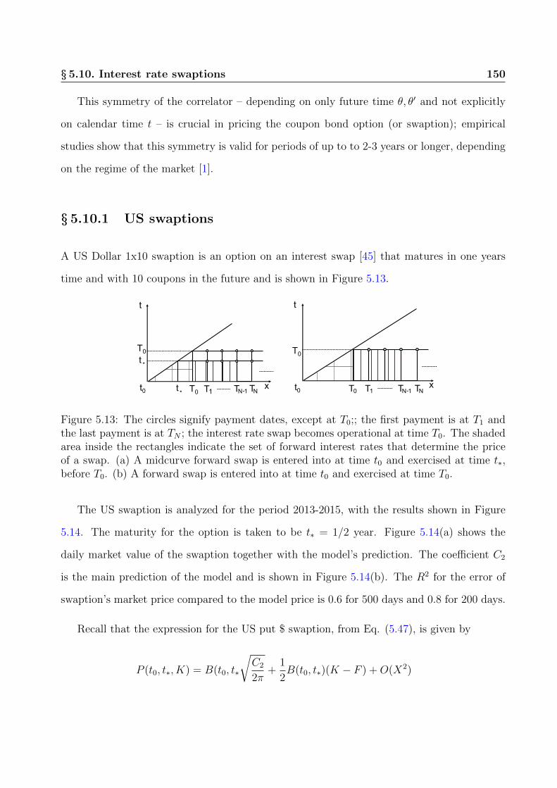
§ 5.10. Interest rate swaptions 150
This symmetry of the correlator – depending on only future time θ, θ′ and not explicitly
on calendar time t – is crucial in pricing the coupon bond option (or swaption); empirical
studies show that this symmetry is valid for periods of up to to 2-3 years or longer, depending
on the regime of the market [1].
§ 5.10.1 US swaptions
A US Dollar 1x10 swaption is an option on an interest swap [45] that matures in one years
time and with 10 coupons in the future and is shown in Figure 5.13.
1 - -
Figure 5.13: The circles signify payment dates, except at T0;; the first payment is at T1 andthe last payment is at TN ; the interest rate swap becomes operational at time T0. The shadedarea inside the rectangles indicate the set of forward interest rates that determine the priceof a swap. (a) A midcurve forward swap is entered into at time t0 and exercised at time t∗,before T0. (b) A forward swap is entered into at time t0 and exercised at time T0.
The US swaption is analyzed for the period 2013-2015, with the results shown in Figure
5.14. The maturity for the option is taken to be t∗ = 1/2 year. Figure 5.14(a) shows the
daily market value of the swaption together with the model’s prediction. The coefficient C2
is the main prediction of the model and is shown in Figure 5.14(b). The R2 for the error of
swaption’s market price compared to the model price is 0.6 for 500 days and 0.8 for 200 days.
Recall that the expression for the US put $ swaption, from Eq. (5.47), is given by
P (t0, t∗, K) = B(t0, t∗
√C2
2π+
1
2B(t0, t∗)(K − F ) +O(X2)

§ 5.10. Interest rate swaptions 151
0 50 100 150 200 250 300 350 400 450 5000.06
0.08
0.1
0.12
0.14
0.16
0.18
0.2
0.22
Red(heavy): data
Blue(light): model
Black(break): model without c2
0 50 100 150 200 250 300 350 400 450 5000.015
0.02
0.025
0.03
0.035
0.04
0.045
Figure 5.14: The daily price of a US Dollar 1x10 swaption for the period 2013-2015. Theheavy (red) line is data. The blue line is the full model value of the swaption with C2 Thebroken line is the value of the swaption withoutthe C2 coefficient. (b) The value of C2 as afunction of time.
consists of two parts: a contribution due to C2 and another contribution that is model inde-
pendent and given by (1/2)B(t0, t∗)(K−F ). Both terms are of the same magnitude and both
are essential. The stochastic behavior of the swaption is captured by (1/2)B(t0, t∗)(K − F );
the C2 coefficient changes the overall drift of the swaption and corrects the behavior of the
model’s price, as shown in Figure 5.14(b) so as to provide an accurate price of the swaption,
as shown in Figure 5.14(a).
0 20 40 60 80 100 120 140 160 180 2000.08
0.09
0.1
0.11
0.12
0.13
0.14
0.15
0.16
0.17
0.18
US Option
Singapore Option depending on US
Singapore Option
0 20 40 60 80 100 120 140 160 180 2000.05
0.1
0.15
0.2
0.25
0.3
US
malaysia1
malaysia2
Figure 5.15: (a) Swaption of US, Singapore stand-alone and Singapore spread interest rates.(b) Swaption of US and stand-alone Malaysian interest rates . Data for the period 12 January2012 to 20 October 2012.

§ 5.10. Interest rate swaptions 152
§ 5.10.2 Singapore swaptions
Let g(t, x) be the Singapore forward yield curve. The quantum finance model for g(t, x) is
based on the assumption that it is driven by the US Dollar yield curve, plus a spread yield
curve given by ξ(t, x), as given in Eq. (5.5). The Singapore bond is given by
Ri = exp−∫ Ti
t∗
dxg(t0, x) ; R =N∑i=1
ciRi
The price of the risky coupon bond put option, from Eq. (5.47), is given
C(t0, t∗, K) = R(t0, t∗)
√C2
2π+
1
2R(t0, t∗)(K −R) +O(X2) (5.50)
with
C2 '∑ij
cicjRiRjGij
The C2 coefficients given in Eq. (5.82) for the risky bond are directly computed from
market correlators and yield the following
Gij =
∫ t∗
t0
dt
∫ Ti−t
t∗−tdθ
∫ Tj−t
t∗−tdθ′
×σ(θ)D(θ, θ′)σ(θ′) + γ(θ)C(θ, θ′)γ(θ′) + 2σ(θ)(D∆C)(θ, θ′)γ(θ′)
(5.51)
Expressing the result given above in Eq. (5.51) directly in terms of the empirically evaluated
correlators yields the following
Gij =
∫ t∗
t0
dt
∫ Ti−t
t∗−tdθ
∫ Tj−t
t∗−tdθ′
×E[δfδf ]c(θ, θ
′) + E[δ(g − f)δ(g − f)]c(θ, θ′) + 2E[δfδ(g − f)]c(θ, θ
′)
(5.52)
§ 5.10. Interest rate swaptions 153
The expression of Gij in terms of the correlators is a result of the general framework
of the quantum finance model for forward interest rates; however, the empirical correlators
themselves are model independent, and encode the full information of the market.
Eq. (5.52) above is evaluated using empirical results. Clearly using the market correlators
will yield more accurate results since a specific choice of an action is calibrated against the
market’s correlators.
Singapore and Malaysian currency based interest rate swaptions are not traded instru-
ments. The price of a swaption given in Eq. (5.47) can be used to generate the model’s
predictions on the value of the Singapore and Malaysian swaptions, and is shown in Figures
5.15(a) and (b).
The Singapore swaptions – for modeling both the spread of the Singapore forward interest
rates above the US forward interest rates as well as for the stand-alone Singapore forward
interest rates – are seen to follow the US swaption values. As can be seen from Figure 5.15(a),
whenever the Singapore swaption value deviates from the US swaption, the value of the
Singapore swaption changes and criss-crosses the US swaption value. It is logical to expect
the US swaption market should drive the value of Singapore swaption, given that the US
swaption is the most liquid instrument and has the greatest range of maturities and coupon
payments.
§ 5.10.3 Malaysian swaptions
The model’s fit for the Malaysian forward interest rates, discussed in Section § 5.8.1, is not
very good with R2 = 0.58; the general framework of quantum finance nevertheless can still be
applied to the Malaysian case. The reason being that the specific form of the action chosen in
Eq. (5.7) is not necessary, and instead one can instead start with a generic propagator for the

§ 5.11. Conclusions 154
action denoted by H−1(θ, θ′) without specifying its dependence on θ, θ′. One can generalize
the action given in Eq. (5.7) to the following
S[A; ξ] = −1
2
∫ ∞t0
dt
∫ ∞t
dxA2(t, x) +
1
µ2(∂A(t, x)
∂x)2 +
1
λ4(∂2A(t, x)
∂x2)2
− 1
2
∫ ∞t0
dt
∫ ∞t
dxM(t, x)− A(t, x)
H−1(θ, θ′)
M(t, x′)− A(t, x′)
+
∫ ∞t0
dt
∫ ∞t
dxdx′∆M(x− t, x′ − t)A(t, x)(M(t, x′)− A(t, x′))
where M(t, x)−A(t, x) yields the spread of the Malaysian over the US forward interest rates.
The earlier analysis for the price of the swaption goes through and one only needs to
empirically evaluate the propagator H(θ, θ′). Gij given in Eq. (5.52) required for pricing a
swaption is evaluated empirically and hence the expression of Gij can be evaluated in terms
of the empirical correlators. Evaluating Gij empirically for the Malaysian swaption, the gen-
eralized quantum finance model’s prediction for the Malaysian swaption, using the Malaysian
empirical propagator, is given in Eq. (5.15)(b).
The Malaysian swaption seems to be fairly insensitive to the movements of the US swap-
tion, which can be attributed to the Malaysian debt market being decorrelated from the
US debt market. The Malaysian swaption’s price is always much higher than the US swap-
tion, which can be explained by the higher risk of Malaysian swaptions compared to the US
sovereign swaptions.
§ 5.11 Conclusions
The study of risky coupon bonds reveals many new features of the forward interest rates of
emerging markets, of which Singapore is one of the more robust examples. The Singapore
forward interest rates were studied both as stand-alone and as being driven by the US forward

§ 5.11. Conclusions 155
interest rates. The empirical study shows that both approaches give reasonable results.
The modeling the Singapore forward interest rates by a spread over the US extends the
quantum finance formulation of forward interest rates to the study of two coupled forward
interest rates as given by the action in Eq. (5.7), with the coupling ∆ being small. This allows
one to study the two rates perturbatively. The extension of the martingale condition for two
coupled forward interest rates leads to new terms for the drift, as in Eq. (5.75), that couple
both the forward interest rates through the spread of the Singapore forward interest rates.
The result of the empirical calibration show that modeling the Singapore forward interest
rates by a spread over the US is more in line with the parameters of the US rates, in contrast
to the value of market time index η from the calibration of the stand-alone US forward interest
rates.
The Malaysian forward interest rates seem to have anomalies not present in the US or
the Singapore case; for this reason, an accurate fit of the model could not be obtained for
the Malaysian case. However, one can extend the model, as discussed in Section § 5.10.3, by
using the quantum finance framework of an action functional and path integrals, by letting
the propagator in the action be determined empirically. Such a generalization of the quantum
finance framework allows one to study the Malaysian forward interest rates and to price its
options – such as the interest rate swaptions and coupon bond call and put options.
In summary, if one is concerned with only the home market, one can model the forward
interest rates as a stand-alone case and ignore its coupling to the international debt market.
However, if an emerging economy wants to issue sovereign debt in the international capital
markets, it is more consistent with the international market to model the emerging markets
debt market as being driven by the US debt markets.

§ 5.12. Appendix 1: Risky coupon bond option 156
§ 5.12 Appendix 1: Risky coupon bond option
The price of the risk free coupon bond option has been evaluated in [1]. The derivation is
generalized to the case of the risky bond.
A coupon bond is a portfolio of zero coupon bonds with fixed coupons an paid out at
pre-determined future times Tn = n`, where ` is the tenor. The risky coupon bond, having a
principal L and maturing at future time TN , is given by
R(t) =N∑i=1
anR(t, Tn) + LR(t, TN) ≡N∑i=1
cnR(t, Tn)
Let C(t) be the price of a call option at time t. A call option for the risky coupon bond,
maturing at future time t∗ and with strike price K, has a payoff function given by [1]
C(t∗) = [R(t∗)−K]+
The price of a call option at time t is defined to be the discounted value of the conditional
expectation value of the payoff function, given the value of the security at time t, which in
our case are the forward interest rates at time t given by g(t, x). There is a wide choice of
instruments that can be used for discounting future cash flows, all of which yield a martingale
evolution of the underlying security. For coupon bond options, the most suitable numeraire
for discounting is the forward bond measure, with the zero coupon bond R(t, t∗) used for
discounting future cash flows. The call option is then given by
C(t0)
R(t0, t∗)= E[
C(t∗)R(t∗, t∗)
] : Martingale condition

§ 5.12. Appendix 1: Risky coupon bond option 157
and which yields the option price at time t0 given by
C(t0) = R(t0, t∗)[R(t∗)−K]+ (5.53)
The risky zero coupon bond is represented as follows
R(t∗, Ti) = exp−∫ Ti
t∗
dxg(t∗, x) = e−βi−QiRi(t0, t∗, Ti) (5.54)
where we make the following defintions
Ri = R(t0, t∗, Ti) = exp−∫ Ti
t∗
dxg(t0, x) (5.55)
Qi =
∫Di
[σ(t, x)A(t, x) + γ(t, x)ξ(t, x)]
≡∫ t∗
t0
dt
∫ Ti
t∗
dx[σ(t, x)A(t, x) + γ(t, x)ξ(t, x)] (5.56)
*
*
Figure 5.16: The shaded area is the domain of integration Ri.
The domain of integration Di is given in Figure 5.16. The coefficient βi, the integrated
form of the forward measure drift, and is fixed (later) by the martingale condition and is given

§ 5.12. Appendix 1: Risky coupon bond option 158
by
βi =
∫Di
β(t, x) =
∫ t∗
t0
dt
∫ Ti
t∗
dxβ(t, x) (5.57)
The payoff requires the price of the coupon bond at time t∗, which is re-written as
N∑i=1
ciR(t∗, Ti) =N∑i=1
ciRi +N∑i=1
ci[R(t∗, Ti)−Ri] ≡ R + V
with forward bond price R =∑i
ciRi =∑i
Ji (5.58)
The break-up of the coupon bond into R + V is based on the fact that all deviations of the
coupon bond from it’s forward price R are due to fluctuations in the forward interest rates
that are controlled by it’s volatility σ(t, x). In fact, V has an order of magnitude equal to
O(σ) + O(γ) and hence an expansion in power of V results in the volatility expansion that
one is aiming for [1].
From Eq. (5.54), the potential is given by
V ≡N∑i=1
ci[R(t∗, Ti)−Ri] =N∑i=1
ci[Rie
−βi−Qi −Ri
]=
N∑i=1
Ji[e−βi−Qi − 1
](5.59)
Hence, from Eqs. (5.56) and (5.59)
V =N∑i=1
Ji[e−βie
−∫Di
(σA+γξ) − 1]
(5.60)
and the payoff function is given by
[ N∑i=1
ciR(t∗, Ti)−K]
+=[R +
N∑i=1
Ji(e−βi−Qi − 1)−K
]+
(5.61)
=[R + V −K
]+

§ 5.12. Appendix 1: Risky coupon bond option 159
The payoff function is re-written using the properties of the Dirac delta function as follows
( N∑i=1
ciR(t∗, Ti)−K)
+=
1
2π
∫ +∞
−∞dpdηeiη(V−p)(F + p−K
)+
The price of the call option, from Eq. (5.53), can be written as
C(t0, t∗, K) = R(t0, t∗)1
2π
∫ +∞
−∞dpdη
(R + p−K
)+e−iηpZ(η) (5.62)
with the partition function for the call option price is given by
Z(η) =1
Z
∫DADξeSeiηV ; Z =
∫DADξeS (5.63)
From the expression for the partition function given above, the effective action for the
pricing of the coupon bond option, from Eqs. (5.60) and (5.63), is given by
SEff ≡ S[A; ξ] + iηV (5.64)
= S[A; ξ] + iηN∑i=1
Ji[e−βi−Qi − 1
]= S[A; ξ] + iη
N∑i=1
Ji[e−βie
−∫Di
(σA+γξ) − 1]
(5.65)
where recall
Ji = ciFi ; Fi = exp−∫ Ti
t∗dxg(t0, x) (5.66)
A cumulant expansion [46] of the partition function in a power series in η yields
Z(η) = eiηC1− 12η2C2−i 1
3!η3C3+ 1
4!η4C4+... (5.67)

§ 5.12. Appendix 1: Risky coupon bond option 160
The coefficients C2, C3, C4, ... are evaluated using Feynman diagrams.
Expanding the right hand side of Eq. (5.63) in a power series to fourth order in η yields
Z(η) =1
Z
∫DADξeiηV eS[A;ξ]
=1
Z
∫DADξeS[A;ξ]
[1 + iηV +
1
2!(iη)2V 2 +
1
3!(iη)3V 3 +
1
4!(iη)4V 4 + · · ·
](5.68)
Comparing Eqs. (5.67) and (5.68) yields, to fourth order in η, the following
C1 = E[V ] (5.69)
C2 = E[V 2]− C21 (5.70)
C3 = E[V 3]− C31 (5.71)
C4 = E[V 4]− 3C22 − C4
1 (5.72)
As shown in [1], the coefficient C1 must be exactly zero to obey the martingale condition for
the forward measure. Hence, the martingale condition fixes the drift β by the requirement
that
C1 = E[V ] =N∑i=1
Ji[EF(e−βi−
∫Di
(σA+γξ))− 1]
= 0 (5.73)
Recall the volatility functions σ, γ are functions of only x− t. Performing the Feynman path
integration yields, in matrix notation
eβi = EF (e−
∫Di
(σA+γξ))=
∫DADξeSe
−∫Di
(σA+γξ)(5.74)
= exp1
2
∫ t∗
t0
dt
∫ Ti
t∗
dx
∫ Ti
t∗
dx′[σ(x− t) , γ(x− t)]M(x− t;x′ − t)
σ(x′ − t)
ξ(x′ − t)

§ 5.12. Appendix 1: Risky coupon bond option 161
Hence the drift is given by
β(x− t) =
∫ x
t
dx′[σ(x− t) , γ(x− t)]M(x− t;x′ − t)
σ(x′ − t)
ξ(x′ − t)
(5.75)
and yields
C1 = 0
The drift α(t, x) for the risk free forward interest rates f(t, x) can be obtained by setting γ to
zero and yields the result given in [1]
α(t, x) =
∫ x
t
dx′σ(x− t)D(x− t;x′ − t)σ(x′ − t)
It is shown in [1] that the put-call parity for the coupon bond requires two conditions
Z(0) = 1 ; C1 = 0
The condition Z(0) = 1 is fulfilled by the normalization of the partition function Z(η) and the
second condition follows from the martingale condition. The call option partition function is
given by
Z(η) = e−12η2C2−i 1
3!η3C3+ 1
4!η4C4... (5.76)
The price of the call option, from Eqs. (5.53) and (5.62)
C(t0, t∗, K) = R(t0, t∗)1
2π
∫ +∞
−∞dpdη
(F + p−K
)+e−iηpZ(η) (5.77)

§ 5.12. Appendix 1: Risky coupon bond option 162
and yields the following for the price of a coupon bond call option [1]
C(t0, t∗, K) = R(t0, t∗)
√C2
2π− 1
2R(t0, t∗)(K − F ) +O(X2) (5.78)
To evaluate C2, using the martingale condition given in Eq. (5.74), we have
C2 = EF [V 2] =N∑ij=1
JiJjEF[(e−βi−
∫Di
(σA+γξ) − 1)(e−βj−
∫Dj
(σA+γξ) − 1)]
⇒ C2 =N∑ij=1
JiJjEF[e−βi−βj−
∫Di
(σA+γξ)−∫Dj
(σA+γξ) − 1]
≡N∑ij=1
JiJj(eGij − 1) '
N∑ij=1
JiJjG2ij : Ji = ciRi (5.79)
Performing the Gaussian integration to evaluate Gij yields two types of terms.
• Terms that depend only on the individual domains Di, Dj. The drifts βi, βj cancel these
term.
• Terms that link domains Di and Dj, and which are generically shown in Figure 5.17
Hence, the C2 coefficient for the risky bond is given by
Gij = G(1)ij +G
(2)ij +G
(3)ij ; θ = x− t ; θ′ = x′ − t (5.80)
G(1)ij =
∫ t∗
t0
dt
∫ Ti
t∗
dx
∫ Tj
t∗
dx′σ(θ)D(θ, θ′)σ(θ′)
G(2)ij =
∫ t∗
t0
dt
∫ Ti
t∗
dx
∫ Tj
t∗
dx′γ(θ)C(θ, θ′)γ(θ′)
G(3)ij = 2
∫ t∗
t0
dt
∫ Ti
t∗
dx
∫ Tj
t∗
dx′σ(θ)(D∆C)(θ, θ′)γ(θ′)
The integration domain for Gij is illustrated in Figure 5.17, and shows it’s dependence on
Ti and Tj. Gij is the forward bond propagator that expresses the correlation in the fluctuations

§ 5.13. Appendix 2: Swaptions 163
t
0t
0t jTiT
Future Time
Cal
endar
Tim
e
jFiF
M(t,x,x’)
x x’
t*
t*
Figure 5.17: The shaded domain of the forward interest rates contribute to Gij. For a typicalpoint t in the time integration, the figure shows the typical correlation function M(x, x′; t)connecting two different values of the forward interest rates at future time x and x′.
of the forward bond prices Fi = F (t0, t∗, Ti) and Fj = F (t0, t∗, Tj). The computation for the
cumulant’s coefficients yields, from Eq. (5.79), the result
C2 'N∑ij=1
JiJjGij +O(σ2γ2, σγ3, σ3γ) (5.81)
The integrations for Gij are written in terms of future time θ = x − t as this is required
for the empirical analysis. Hence, we obtain
Gij =
∫ t∗
t0
dt
∫ Ti−t
t∗−tdθ
∫ Tj−t
t∗−tdθ′
× σ(θ)D(θ, θ′)σ(θ′) + γ(θ)C(θ, θ′)γ(θ′) + 2σ(θ)(D∆C)(θ, θ′)γ(θ′) (5.82)
§ 5.13 Appendix 2: Swaptions
Interest swaptions are studied in detail in [7] and we summarize the results.
To quantify the value of the swap, let the swap start at Libor time T0, with payments
made at fixed times Tn = T0 + n`, with n = 1, 2, ..., N ; the first payment is made at T1 and

§ 5.13. Appendix 2: Swaptions 164
the last payment is made at time TN + `TN . Summing upIn summary, at time t0, the values
of the forward swaplets – corresponding to the interest rate payments made at future times
Tn – yields the following forward price for the floating rate receiver swap
swapL(t0, RS) = `VN∑n=0
N − 1B(t0, Tn + `)[L(t0, Tn)−RS
](5.83)
and fixed rate receiver swap
swapR(t0, RS) = `VN∑n=0
N − 1B(t0, Tn + `)[RS − L(t0, Tn)
](5.84)
They obey the identity
swapL(t0, RS) + swapR(t0, RS) = 0 (5.85)
One can simplify the expression for the swaps. The Libor Zero Coupon Yield Curve
represents Libor in terms of Libor zero coupon bonds, and yields [1]
L(t, T ) =1
`
B(t, T )−B(t, T + `)
B(t, T + `)
Hence
`V
N∑n=0
N − 1B(t0, Tn + `)L(t0, Tn) = V
N∑n=0
N − 1[B(t0, Tn)−B(t0, Tn + `)
]= V
[B(t0, T0)−B(t0, TN + `TN)
]Hence, from Eq. (5.83)
swapL(t0, RS) = V[B(t0, T0)−B(t0, TN + `TN)− `RS
N∑n=0
N − 1B(t0, Tn + `)]
(5.86)

§ 5.13. Appendix 2: Swaptions 165
with a similar expression for swapR.
An interest rate swaption, denoted by CL and CR, is an option on a floating or a fixed
interest rate receiver swap, swapL and swapR, respectively.
Consider a swap with N payments dates given by Tn = T0 + n` ; n = 1, 2...., N ; the swap
starts at time T0, the first payment is made at time T1 and the last payment is made at time
TN + `TN . A midcurve swaption, similar to a midcurve caplet, is contracted at time t0 and
matures at time t∗ < T0. The payoff function for a midcurve swaption is given in Figure
5.13(a) and is the same as a midcurve forward swap. The swaption is an option on the swap
and hence has the same cash flow as a swap if it is exercised.
The swaption that will studied henceforth is the one that matures at t∗ = T0, when
the swap becomes operational and is shown in Figure 5.13(b). Almost all market data on
swaptions is exclusively given for this case and is, consequently, the most important one for
empirical studies of swaptions.
The swaption, on maturing, will be exercised only if the value of the swap at time T0 is
greater than it’s initial par value of zero. Hence, the payoff function for the swaption for the
floating and fixed receivers swap, from Eqs. (5.83) and (5.84), is given respectively by the
following
CL(T0, T0;RS) =[swapL(t0, RS)
]+
= `V[ N∑n=0
N − 1B(t0, Tn + `)(L(t0, Tn)−RS)]
+(5.87)
CR(t, T0, RS) =[swapR(t0, RS)
]+
= `V[ N∑n=0
N − 1B(t0, Tn + `)(RS − L(t0, Tn)
)]+
(5.88)

§ 5.13. Appendix 2: Swaptions 166
In terms of zero coupon bonds, the swaption payoff function, from Eq. (5.86), is given by
CL(t0, T0;RS) = V[B(t0, T0)−B(t0, TN)− `RS
N∑n=1
B(t, T0 + n`)]
+(5.89)
and a similar expression for CR. The value of the swaption at an earlier time t < T0 can be
obtained by discounting the payoff function using the money market numeraire and yields
CL(t0, T0, RS) = V E[e−
∫ T0t0
r(t′)dt′CL(T0;RS)]
= V E[e−
∫ T0t0
r(t′)dt′(B(t0, T0)−B(T0, TN)− `RS
N∑n=1
B(T0, T0 + n`))
+
](5.90)
and similarly for CR(t, T0, RS). One can see that a swap is equivalent to a particular portfolio
of coupon bonds, and all techniques that are used for coupon bonds options can be used for
analyzing swaptions.
Discounting by the forward bond numeraire B(t, T0), similar to the case of coupon bond
options given in Eq. (5.53), makes the swaption price computationally more tractable; the
price of the swaption, from Eq. (5.89), is given by
CL(t, T0, RS)
B(t, T0)= V E
[CL(T0;RS)
]⇒ CL(t, T0, RS) = V B(t, T0)E
[B(t, T0)−B(t, TN)− `RS
N∑n=1
B(t, T0 + n`)]
+(5.91)
A change of numeraire changes the drift for the forward interest rates [1].
§ 5.14. Appendix 3: Black’s Model for Swaption 167
§ 5.14 Appendix 3: Black’s Model for Swaption
Market data for swaptions, including the data provided by Bloomberg, is quoted as an effective
volatility for the swaption based on Black’s model – similar to the implied volatility surface
being provided for the price of vanilla stock options. From the effective volatility, the swaption
price can be re-constructed. Hence, to obtain the empirical value of the swaptions, we briefly
discuss Black formula for a swaption [47].
Consider coupon payments paid at fixed times Ti = `i. In our case ` = 90 days. Tn is the
time for each payment. m is the times of swaption payments per year; we take m = 2 for
semiannual swaptions. The total number of payments is N . The last payment of the coupon
bond, which includes the payment of the principal, is given at time TN . Hence
N = mn ; TN = `mn (5.92)
The payer swaption has the value, at time t when it is issued, given by [1]
Cps (t) = V [swap(t)]+
For payments at equal time intervals Ti − Ti−1 = `, which is the period for each fixed
payment, the swaption is given by
Cps (t) = V
[R(t, T0)−R(t, TN)− `Rk
N∑i=1
R(t, Ti)]]
+
Let Πt = Cps (t) be the value of the payer swaption at present time t; we use `L
∑Ni=1R(t, Ti)
as the numeraire. The discounted value of payoff function of an option maturing at future

§ 5.14. Appendix 3: Black’s Model for Swaption 168
time t∗ is given by
Πt
`L∑N
i=1R(t, Ti)= E[t,t∗]
[ Cps (t∗)
`L∑N
i=1R(t∗, Ti)
]= V E[t,t∗]
[[R(t∗, T0)−R(t∗, TN)]− `Rk
∑Ni=1R(t∗, Ti)+
`L∑N
i=1R(t∗, Ti)
]= E[t,t∗][
R(t∗, T0)−R(t∗, TN)
`∑N
i=1R(t∗, Ti)−Rk+]
= E[t,t∗]
[S(t∗, T0, TN)−Rk
]+
The forward swap rate S is defined as
S(t, T0, TN) =R(t, T0)−R(t, TN)
`∑N
i=1R(t, Ti)(5.93)
The Black-76 model for the value of the swaption is based on the assumtion that forward
swap rate S follows a geometric Brownian Motion with constant volatility. The value of the
swaption is given by
Πt = `V( N∑i=1
R(t, Ti))× E[t,t∗]
[S(t∗, T0, TN)−Rk
]+
(5.94)
Based on the Black-Scholes analysis, the value of swaption is given by the following
Cs(t) = `V( N∑i=1
R(t, Ti))× [S(t, T0, TN)N(d1)−RkN(d2)] (5.95)
where N(x) is the cumulative normal distribution with
d1 =ln(S(t, T0, TN)/Rk) + 1
2σ2T
σ√T
; T = t∗ − t (5.96)
d2 = d1 − σ√T (5.97)

§ 5.15. Appendix 4: Zero coupon bonds from coupon bonds 169
Bloomberg provides the daily value of σ as well as the fixed value of the fixed leg of the
swaption, given by Rk. The daily value of the zero coupon bonds R(t, Ti) are available from
Bloomberg, and one can then compute the daily price of the swaption using Eq. (5.95).
§ 5.14.1 Par value of fixed payments
The forward price, at time t0 for a swaption maturing at time t∗ is given by
Cps (t, t∗;Rk) = L
[F (t, t∗, T0)− F (t, t∗, TN)− `Rk
N∑i=1
F (t, t∗, Ti)]
+
where the forward bond price is given by
F (t, t∗, Ti) = exp−∫ Ti
t∗
dxf(t, x)
The par value RP of the swaption is given by the forward swaption being zero. Hence
Cps (t0, t∗;RP ) = 0
and yields
`RP =F (t0, t∗, T0)− F (t0, t∗, TN)∑N
i=1 F (t0, t∗, Ti)
§ 5.15 Appendix 4: Zero coupon bonds from coupon
bonds
In this Section, we discuss how to use the boot-strapping method to extract the zero coupon
bonds from coupon bonds. The data provider, such as Bloomberg, gives the yield to maturity
§ 5.15. Appendix 4: Zero coupon bonds from coupon bonds 170
yi(t) (YTM), every day t and for the coupon payments at future time, specified by i.3
Consider a coupon bond, denoted by CN(t). The coupons can be annual, semi-annual or
quarterly; a coupon bond have coupons that are paid pay quarterly, semiannual or annual. As
in Eq. (5.92), define ` = 90 days. Payments can be made annually, semiannually or quarterly,
and yield the following
N = mn ; TN = `mn : m = 4 annual ; m = 2 semiannual ; m = 1 quarterly
Note that the maturity of the bond is given by n = TN/(`m), m` is the tenor of the coupon
bond, N is the total number of payments and TN is the total number of years for the coupon
bond to expire. The coupon payments are made at times
Ti = `mi ; i = 1, 2, · · · , N
The coupon bond pays N fixed coupons at time Ti = `mi, with the final payment made
at time TN . The principal L is returned the end of TN years. The price of the coupon bond
is the sum is the sum of the discounted future cash flows. Fix t = 0 and let the coupon for
the ith payment be fixed at ci; the coupon bond has the following expansion in terms of the
zero coupon bonds
CN(t) =N∑i=1
ciB(t, Ti) + LB(t, TN)
=N∑i=1
ci(1 + 1
myi(t))i
+L
(1 + 1myN(t))N
(5.98)
where the YTM discounting factor yi(t) is given yearly. Hence, in terms of the discounting
3Some data providers give the price of the coupon bond by varying the coupons ci so that the bond hasits the par value. We will not analyze this case.

§ 5.15. Appendix 4: Zero coupon bonds from coupon bonds 171
factors, the zero coupon bond is given by
B(t, Ti) =1
(1 + 1myi(t))i
(5.99)
The price of a coupon bond CN(t) = CN is written in terms of yield to maturity (YTM)
y(t) = y by the following equation
CN(t) ≡ CN =c1
1 + 1my
+c2
(1 + 1my)2
+ · · · cn(1 + 1
my)N
+L
1m
(1 + y)N(5.100)
If the coupon if fixed at cn = c, we have
CN(y) =c
y/m+y/m− c/L
y/m· L
(1 + y/m)N(5.101)
The par value of YTM is y/m = c/L and the price of the bond is then equal to its face value
L. In other words
CN(y) = L : y = cm/L = par YTM
The data is usually given by the yield to maturity y = y(t); hence
CN(y(t)) : price of coupon bond
Each issuer of coupon bonds, be it a sovereign bond or a corporate bond, has its own
complete forward yield curve. The price for the coupon bond of a given issuer is provided by
the data provider by specifying all the coupons cn as well as giving the daily price using the
YTM y(t).
Consider a coupon bond with one payment of coupon c1 and let the YTM be y(t) = y;

§ 5.15. Appendix 4: Zero coupon bonds from coupon bonds 172
then, from Eqs. (5.98) and (5.100)
C1 =c1
(1 + 1my1)
+L
(1 + 1my1)
=c1
(1 + 1my)
+L
(1 + 1my)⇒ y1 = y : y1 is fixed
For a coupon bond with two payments, let the coupons be c1, c2 and let the YTM be y; one
has, from Eqs. (5.100) and (5.98)
c2
(1 + 1my)2
+c1
(1 + 1my)
+L
(1 + 1my)2
= C2 =c2
(1 + 1my2)2
+c1
(1 + 1my1)
+L
(1 + 1my2)2
⇒ c2 + L
(1 + 1my2)2
=c2
(1 + 1my)2
+c1
(1 + 1my)
+L
(1 + 1my)2− c1
(1 + 1my1)
: y2 is fixed
Similar to above relation, once the values of y1, y2, · · · , yn−1 have been evaluated, the value of
yn can be determined recursively.
Hence, of all the discounting factors y1, y2, · · · , yn, · · · , yN can be obtained from the price
of coupon bonds C1, C2, · · · , CN with the different of coupon payments given by c1, c2, · · · , cN .
We can then obtain the zero coupon bond from Eq. (5.99).
In general, for coupons cn and for time t in between Tm−1 and Tm, the coupon bond price
is given in terms of YTM y by the following
CN(t) = (1 +1
my)t−Tm−1
×(
cm(1 + 1
my)1
+cm+1
(1 + 1my)2
+ ...+cN
(1 + 1my)N−m+1
+L
(1 + 1my)N−m+1
)Tm−1 ≤ t ≤ Tm
Suppose that the data is given in a manner in which the maturity of the coupon bond is
always at a fixed θi = t + Ti. The coupon bond then has a price, similar to Eq. (5.98), at

§ 5.16. Appendix 5: Forward interest rates and zero coupon bonds 173
time t given by
CN(t) =N∑i=1
ciB(t, t+ Ti) + LB(t, t+ TN) ; ciL = αi
CN(t)
L=
N∑i=1
αi(1 + 1
myi(θi))i
+1
(1 + 1myN(θN))N
; θi = t+ Ti (5.102)
The yield to maturity yi(θi) can be extracted exactly as the case where the coupon bond
data is given with coupon bonds have a fixed maturity. Eq. (5.99) is then modified to yield
the zero coupon bond as follows
B(t, t+ Ti) =1
(1 + 1myi(t+ Ti))i
= exp−∫ t+Tn
t
dxf(t, x) = exp−∫ Tn
0
dθf(t, θ)(5.103)
§ 5.16 Appendix 5: Forward interest rates and zero coupon
bonds
The forward interest rates are sometimes given directly, as is the case for the US. In other
cases, the price of coupon bonds for different maturities is given, from which the zero coupon
bond price can be obtained as discussed in Section § 5.15 and given in Eq. (5.99).
In this Section, the forward interest rates f(t, x) are obtained from the price of zero coupon
bonds B(t, Tn).
Consider a collection of zero coupon bonds B(t, Tn) maturing at future time Tn in the
future. Let the present time t = 0 to simplify the notation, and define
B(0, Tn) ≡ B(Tn) ; f(0, x) ≡ f(x)

§ 5.16. Appendix 5: Forward interest rates and zero coupon bonds 174
The forward interest rates, from Eq. (5.99) (suppressing the index t = 0) are given by
B(Tn) = exp−∫ Tn
0
dxf(x) =1
(1 + 1myn)n
(5.104)
The future times Tn define a lattice for the zero coupon bond. The forward interest rates
are defined on the future lattice in the following manner
f(x) = fn(x) ; x ∈ [Tn−1, Tn]
The forward interest rates and the corresponding future times are shown as the Figure 5.18.
Hence
B(Tn) = exp−N∑n=1
∫ Tn
Tn−1
dxfn(x)
and
ln(B(Tn−1)
B(Tn)) =
∫ Tn
Tn−1
dxfn(x)
Note that
................0 1 2 N-1 N
f1 f
2 ................ f
N
T1 T
2 ................. T
N-1 T
N
Figure 5.18: Forward interest rate and future time lattice.
The forward interest rates are assumed, piecewise, to be second order polynomials and
given below
fn(x) = an + bnx+ cnx2 (5.105)

§ 5.16. Appendix 5: Forward interest rates and zero coupon bonds 175
Hence
ln(B(Tn−1)
B(Tn)) =
∫ Tn
Tn−1
dxfn(x)
= an(Tn − Tn−1) +1
2bn(T 2
n − T 2n−1) +
1
3cn(T 3
n − T 3n−1) (5.106)
Let
f ′n−1(Tn) =dfn−1(x)
dx
∣∣∣x=Tn
For each period from Tn−1 to Tn, to ensure that the forward interest rates yield a smooth
function for f(x), the following conditions are imposed.
• fn−1(Tn) = fn(Tn) : forward interest rates are continuous. Hence
an−1 + bn−1Tn + cn−1T2n = an + bnTn + cnT
2n (5.107)
• f ′n−1(Tn) = f ′n(Tn) : forward interest rates first derivatives are continuous. Hence
bn−1 + 2cn−1Tn = bn + 2cnTn (5.108)
We count the number of independent equations that the scheme provides.
• There are N conditions are in Eq. (5.106).
• The boundary conditions given in Eqs. (5.107) and (5.108) are for points from 1 to
N − 1, and hence yield 2(N − 1) conditions.
• One more conditions is that the spot interest rate r is obtained from the market. Using
f(t, t) = r yields
f1(0) = r = a1 (5.109)
§ 5.16. Appendix 5: Forward interest rates and zero coupon bonds 176
• The last condition is the Neumann condition at the end point, that is f ′N(TN) = 0; this
follows from the fact that the final value of the interest rate is taken to be random.
Hence
f ′N(TN) = 0 = bN + 2cNTN (5.110)
In summary, from Eqs. (5.106), (5.107), (5.108), (5.109) and (5.110), the number of
equation we have is
N + 2(N − 1) + 2 = 3N
and this is sufficient to fix the 3N unknown parameters an, bn, cn.
There are 3N parameters and 3N linear equations. These linear equation are written as
AX = b, where the matrix A is defined by Eqs. (5.106), (5.107), (5.108), (5.109) and (5.110)
and given below. The structure of matrix A is in overlapping blocks of size 3x6 and organized
as shown in Figure 5.19. More precisely, each block has the following entries
• The first row is the continuity equation given in Eq. (5.107). The first entry A11 = 1 is
due to the boundary condition given in Eq. (5.109). In general, there are 6 entries to
this row.
• The second row enters the data given in Eq. (5.106). In general, there are 3 entries to
this row.
• The third row is the condition given in Eq. (5.108), with 4 entries per row. The last
row of A encodes the boundary condition given in Eq. (5.110).
The matrix structure of A is shown in Figure 5.19.

§ 5.16. Appendix 5: Forward interest rates and zero coupon bonds 177
. . . . . .
. . . . . .
3 conditions
6 parameters
A=
Figure 5.19: The 3x6 block structure, with three elements overlapping between successiverows, is shown in the figure.
The matrix elements are written as follows.
1 2 3 4 5 6 ... 3n− 2 3n− 1 3n 3n+ 1 3n+ 2 3n+ 3 ... 3N − 2 3N − 1 3N
1 0 0 0 0 0... 0 0 0 0 0 0... 0 0 0
T112T
21
13T
31 0 0 0... 0 0 0 0 0 0... 0 0 0
0 1 2T1 0 −1 −2T1... 0 0 0 0 0 0... 0 0 0
... ... ... ... ... ...... ... ... ... ... ... ...... ... ... ...
... ... ... ... ... ...... 1 Tn T 2n −1 −Tn −T 2
n ... 0 0 0
... ... ... ... ... ...... 0 0 0 Tn − Tn−112(T 2
n − T 2n−1) 1
3(T 3n − T 3
n−1) 0 0 0
... ... ... ... ... ...... 0 1 2Tn 0 −1 −2Tn... 0 0 0
... ... ... ... ... ...... ... ... ... ... ... ...... ... ... ...
... ... ... ... ... ...... 0 0 0 0 0 0... 0 1 2TN

§ 5.16. Appendix 5: Forward interest rates and zero coupon bonds 178
×
a1
b1
c1
...
an−1
bn−1
cn−1
an
bn
cn
...
aN
bN
cN
=
r
ln(B(0)/B(T1))
0
...
0
0
ln(B(Tn − 1)/B(Tn))
...
0
The solution to the forward interest rates determination is given by
AX = b ⇒ X = A−1b (5.111)
From N data points, we could obtain a fit with 3N parameters for the forward interest rates, and
hence obtaining a far superior result that using only the N data points would yield. The reason being

§ 5.16. Appendix 5: Forward interest rates and zero coupon bonds 179
we used the continuity and differentiability of the forward interest rates, and in this way encoding
more information into the fit for the forward interest rates. One can of course, use a higher power
fit to get even better results, but in our studies we find the quadratic fit to be adequate [48].

Bibliography
[1] Belal E. Baaquie. Interest Rates and Coupon Bonds in Quantum Finance. Cambridge
University Press, UK, 1st edition, 2010.
[2] Simon Benninga et al. Financial modeling. MIT Press Books, 1, 2008.
[3] Belal E Baaquie. Path Integrals and Hamiltonians: Principles and Methods. Cambridge
University Press, 2014.
[4] Belal E Baaquie, Xin Du, and Winson Tanputraman. Empirical microeconomics action
functionals. Physica A: Statistical Mechanics and its Applications, 428:19–37, 2015.
[5] B. E. Baaquie and Cao Yang. Option volatility and the acceleration lagrangian. Physica
A, 393:337–363, 2014.
[6] F. Black and M. Scholes. The pricing of options and corporate liabilities. Journal of
Political Economy, (bf 81):637–654, 1973.
[7] Belal E Baaquie. Quantum finance: Path integrals and Hamiltonians for options and
interest rates. Cambridge University Press, 2004.
[8] D. Heath, R. Jarrow, and A. Morton. Bond pricing and the term structure of interest
rates: A new methodology for contingent claim valuation. Econometrica, 60:77–105,
1992.
i
BIBLIOGRAPHY ii
[9] Belal E. Baaquie. Statistical microeconomics. Physica A: Statistical Mechanics and
its Applications, 392(19):4400 – 4416, 2013. ISSN 0378-4371. URL http://www.
sciencedirect.com/science/article/pii/S0378437113004135.
[10] Jean-Philippe Bouchaud and Marc Potters. Theory of financial risk and derivative pricing:
from statistical physics to risk management. Cambridge university press, 2003.
[11] William Baumol and Alan Blinder. Microeconomics: Principles and policy. Cengage
Learning, 2015.
[12] Hal Varian. Microeconomic theory. W. W. Norton & Company, New York, 1992.
[13] Harold L Cole and Maurice Obstfeld. Commodity trade and international risk sharing:
How much do financial markets matter? Journal of Monetary Economics, 28(1):3–24,
1991.
[14] Emmanuel Haven and Andrei Khrennikov. Quantum social science. Cambridge University
Press, 2013.
[15] Andrei Khrennikov. Quantum-like microeconomics: Statistical model of distribution of
investments and production. Physica A: Statistical Mechanics and its Applications, 387
(23):5826–5843, 2008.
[16] Rosario N Mantegna and H Eugene Stanley. Introduction to econophysics: correlations
and complexity in finance. Cambridge university press, 1999.
[17] Vasiliki Plerou, Parameswaran Gopikrishnan, Bernd Rosenow, Luıs A Nunes Amaral,
and H Eugene Stanley. Universal and nonuniversal properties of cross correlations in
financial time series. Physical Review Letters, 83(7):1471, 1999.

BIBLIOGRAPHY iii
[18] Ole E Barndorff-Nielsen. Econometric analysis of realized volatility and its use in esti-
mating stochastic volatility models. Journal of the Royal Statistical Society: Series B
(Statistical Methodology), 64(2):253–280, 2002.
[19] A Ian McLeod. Distribution of the residual cross-correlation in univariate arma time
series models. Journal of the American Statistical Association, 74(368):849–855, 1979.
[20] Thomas F Cargill and Gordon C Rausser. Temporal price behavior in commodity futures
markets. The Journal of Finance, 30(4):1043–1053, 1975.
[21] William G Tomek. Commodity futures prices as forecasts. Review of Agricultural
Economics, pages 23–44, 1997.
[22] Aaron Smith. Partially overlapping time series: a new model for volatility dynamics in
commodity futures. Journal of Applied Econometrics, 20(3):405–422, 2005.
[23] Robert S Pindyck. The dynamics of commodity spot and futures markets: a primer. The
Energy Journal, pages 1–29, 2001.
[24] Scott H Irwin and Dwight R Sanders. Index funds, financialization, and commodity
futures markets. Applied Economic Perspectives and Policy, 33(1):1–31, 2011.
[25] Belal E Baaquie, Yu Miao, and Xin Du. Multiple commodities in statistical microeco-
nomics: Model and market. Physica A: Statistical Mechanics and its Applications, 462:
912–929, 2016.
[26] P.D. Mannheim. Comprehensive solution to the cosmological constant, zero-point energy,
and quantum gravity problems. Gen. Rel. Gravitation, page 703, 2011.
[27] P.D. Mannheim. Making the case for conformal gravity. Foundations of Physics, page
532, 2011.
BIBLIOGRAPHY iv
[28] S. W. Hawking and Thomas Hertog. Living with ghosts. Phys. Rev. D, 65:103515, May
2002. URL http://link.aps.org/doi/10.1103/PhysRevD.65.103515.
[29] Michele Fontanini and Mark Trodden. Tackling higher derivative ghosts with the eu-
clidean path integral. Phys. Rev. D, 83:103518, May 2011. URL http://link.aps.org/
doi/10.1103/PhysRevD.83.103518.
[30] Lisa Borland. Option pricing formulas based on a non-gaussian stock price model.
Physical review letters, 89(9):098701, 2002.
[31] Vito Latora, Andrea Rapisarda, and Constantino Tsallis. Non-gaussian equilibrium in a
long-range hamiltonian system. Physical Review E, 64(5):056134, 2001.
[32] Mark B Garman and Steven W Kohlhagen. Foreign currency option values. Journal of
international Money and Finance, 2(3):231–237, 1983.
[33] Lishang Jiang and Canguo Li. Mathematical modeling and methods of option pricing.
World Scientific, 2005.
[34] J Orlin Grabbe. The pricing of call and put options on foreign exchange. Journal of
International Money and Finance, 2(3):239–253, 1983.
[35] Paul Wilmott, Jeff Dewynne, and Sam Howison. Option pricing: mathematical models
and computation. Oxford financial press, 1993.
[36] B. E. Baaquie and Cui Liang. American option pricing for interest rate caps and coupon
bonds in quantum finance. Physica A, 38:285–316, 2007.
[37] Belal E. Baaquie, Xin Du, and Jitendra Bhanap. Option pricing: Stock price, stock veloc-
ity and the acceleration lagrangian. Physica A: Statistical Mechanics and its Applications,
416:564 – 581, 2014. ISSN 0378-4371. URL http://www.sciencedirect.com/science/
article/pii/S0378437114007778.

BIBLIOGRAPHY v
[38] Francis A Longstaff. Option pricing and the martingale restriction. Review of Financial
Studies, 8(4):1091–1124, 1995.
[39] Pan Tang, Belal E Baaquie, Xin Du, and Ying Zhang. Linearized hamiltonian of the
libor market model: analytical and empirical results. Applied Economics, 48(10):878–
891, 2016.
[40] Jesus Saa-Requejo and Pedro Santa-Clara. Bond pricing with default risk. Finance, 1997.
[41] Don M Chance. Default risk and the duration of zero coupon bonds. The journal of
finance, 45(1):265–274, 1990.
[42] Robert A Jarrow and Stuart M Turnbull. Pricing derivatives on financial securities
subject to credit risk. The journal of finance, 50(1):53–85, 1995.
[43] Robert C Merton. On the pricing of corporate debt: The risk structure of interest rates.
The Journal of finance, 29(2):449–470, 1974.
[44] CH Hui and CF Lo. A note on risky bond valuation. International Journal of Theoretical
and Applied Finance, 3(03):575–580, 2000.
[45] Ravi Jagannathan, Andrew Kaplin, and Steve Sun. An evaluation of multi-factor cir
models using libor, swap rates, and cap and swaption prices. Journal of Econometrics,
116(1):113–146, 2003.
[46] J. Zinn-Justin. Quantum Field Theory and Critical Phenomenon. Oxford University
Press, UK, 1993.
[47] Bram van den Hoek. Alternative swaption valuation methods. Tilburg University, 2012.
[48] Ken Adams. Smooth interpolation of zero curves. Algo Research Quarterly, 4(1/2):
11–22, 2001.


![arXiv:1903.10507v1 [astro-ph.EP] 25 Mar 2019vironments. We know that stars in di erent parts of the sky and di erent birth environments have di erent properties (West et al. 2008;](https://static.fdocuments.net/doc/165x107/5fe721e5415617432f159b0f/arxiv190310507v1-astro-phep-25-mar-2019-vironments-we-know-that-stars-in-di.jpg)
