Fungicide dose-response trials in wheat: the basis for ...
119
Project Report No. 373 September 2005 Price: £5.00 Fungicide dose-response trials in wheat: the basis for choosing ‘Appropriate Dose’ by D. Lockley 1 and W.S. Clark 2 1 ADAS Mamhead, Exeter, EX6 8HD 2 ADAS Boxworth, Cambridge, CB3 8NN This is the final report of HGCA-funded Project No. 2497 which started in May 2001, lasted for 38 months and was funded with a contract £289,379. It was then extended for a further 12 months by a contract of £82,320. The work was co-ordinated by N D Paveley, ADAS High Mowthorpe. Participants included S Oxley, SAC Edinburgh, A Ainsley, York, M Self, TAG, Morley, W S Clark, ADAS, Boxworth and K D Lockley, ADAS, Mamhead. The Home-Grown Cereals Authority (HGCA) has provided funding for this project but has not conducted the research or written this report. While the authors have worked on the best information available to them, neither HGCA nor the authors shall in any event be liable for any loss, damage or injury howsoever suffered directly or indirectly in relation to the report or the research on which it is based. Reference herein to trade names and proprietary products without stating that they are protected does not imply that they may be regarded as unprotected and thus free for general use. No endorsement of named products is intended nor is it any criticism implied of other alternative, but unnamed, products.
Transcript of Fungicide dose-response trials in wheat: the basis for ...
Project Report No. 373 September 2005 Price: £5.00
Fungicide dose-response trials in wheat: the basis for
choosing ‘Appropriate Dose’
by
D. Lockley 1 and W.S. Clark 2
1ADAS Mamhead, Exeter, EX6 8HD 2ADAS Boxworth, Cambridge, CB3 8NN
This is the final report of HGCA-funded Project No. 2497 which started in May 2001, lasted for 38 months and was funded with a contract £289,379. It was then extended for a further 12 months by a contract of £82,320. The work was co-ordinated by N D Paveley, ADAS High Mowthorpe. Participants included S Oxley, SAC Edinburgh, A Ainsley, York, M Self, TAG, Morley, W S Clark, ADAS, Boxworth and K D Lockley, ADAS, Mamhead. The Home-Grown Cereals Authority (HGCA) has provided funding for this project but has not conducted the research or written this report. While the authors have worked on the best information available to them, neither HGCA nor the authors shall in any event be liable for any loss, damage or injury howsoever suffered directly or indirectly in relation to the report or the research on which it is based. Reference herein to trade names and proprietary products without stating that they are protected does not imply that they may be regarded as unprotected and thus free for general use. No endorsement of named products is intended nor is it any criticism implied of other alternative, but unnamed, products.

CONTENTS
PAGE
ABSTRACT 1
1.0 SUMMARY 2
2.0 INTRODUCTION 3
2.1 The dose-response curve 3
2.2 The recommended dose 4
2.3 Appropriate fungicide doses 4
2.4 Variation in dose-response curves 5
3.0 MATERIALS AND METHODS 7
3.1 Sites 7
3.2 Site selection and establishment 8
3.3 Experiment design 8
3.4 Fungicide treatments 8
3.5 Assessments and records 22
3.6 Data handling 23
3.7 Statistical analysis 23
4.0 RESULTS 25
4.1 Stagonospora nodorum experiments 25
4.2 Yellow rust experiments 43
4.3 Septoria tritici experiments 67
4.4 Brown rust experiments 96
4.5 Mildew experiments 104
5.0 CONCLUSIONS 112
Appendix 1 List of active ingredients and products 116
Appendix 2 List of products and active ingredients 117
1
ABSTRACT
Robust, comparative dose-response data sets were produced for the most widely used fungicides applied to
wheat in the UK. This includes active ingredients from azole, morpholine, strobilurin, spiroketalamine,
benzamide and carboxanilide fungicide groups. Up to three years of data on fungicides launched in 2005 were
obtained from these experiments. These included boscalid (in mixture with epoxiconazole in Tracker),
dimoxystrobin (in mixture with epoxiconazole in Swing Gold), fluoxastrobin (in mixture with prothioconazole
in Fandango), metrafenone (Flexity) and prothioconazole (Proline).
Information on these new products was published in the ‘Wheat Disease Management Guide - 2005
Update‘(published in February 2005) and on the HGCA web site (www.hgca.com) as an interactive tool in
March 2005.
Data on strobilurin performance against S. tritici clearly show a dramatic reduction in efficacy over the period
2002 – 2004. Despite measurements of the frequency of the resistance allele (G143A) conferring resistance to
strobilurin fungicides indicating that resistance levels in the UK were generally 80-100%, there was still a
measurable effect of strobilurin fungicides against S. tritici in these experiments. This phenomenon is not fully
understood.
Analysis of data since 1994 indicates a significant reduction in the activity of epoxiconazole (and by inference,
all other azole fungicides) against S. tritici. The observation of this effect in field trials was supported by
laboratory-based data showing changes in the sensitivity of isolates of S. tritici.
In spite of these changes in sensitivity in populations of mildew and S. tritici, most pathogens attacking wheat
crops are well-controlled by modern fungicides. The main pathogen of wheat, S. tritici, is well controlled by the
azole fungicides, chlorothalonil and boscalid. The morpholines, in mixture with azoles, also add to the control
of septoria. Although control of mildew by the strobilurin fungicides has almost been lost completely in the last
few years, it is still well controlled by cyprodinil, metrafenone, the morpholines, quinoxyfen, and spiroxamine.
The azoles also still add to mildew control. Yellow and brown rust are well controlled by many of the azole and
strobilurin fungicides.
Data from experiments were used to fit exponential curves describing the effect of fungicides on disease, green
leaf area, yield and grain quality. These data typically explained a very high proportion (over 90%) of the
variance. The fitted curves and their parameters are given in the report.

2
1.0 SUMMARY
Within the period of experimentation in this project there was a loss of activity of the strobilurins against
wheat powdery mildew and Septoria tritici. This had a dramatic effect on the efficacy of these products.
Analysis of data from the appropriate dose experiments since 1994 also showed a decline in activity of the
azole fungicides against S. tritici.
Robust, comparative dose-response data sets were gathered for the most widely used fungicides applied to
wheat. This includes active ingredients from azole, morpholine, strobilurin, spiroketalamine, benzamide
and carboxanilide fungicide groups. Up to three years of data on fungicides launched in 2005 were
gathered. These included boscalid (in mixture with epoxiconazole in Tracker), dimoxystrobin (in mixture
with epoxiconazole in Swing Gold), fluoxastrobin (in mixture with prothioconazole in Fandango),
metrafenone (Flexity) and prothioconazole (Proline).
Data on strobilurin performance against S. tritici clearly show a dramatic reduction in efficacy from 2002 to
2004. In other HGCA LINK experiments, measurements of the frequency of the resistance allele (G143A)
in the population of S. tritici indicated that resistance levels were generally greater than 80%. However, in
these experiments there was still a measurable effect of strobilurin fungicides against S. tritici.
Analysis of data since 1994 indicates a significant reduction in activity of epoxiconazole (and by inference,
all other azole fungicides) against S. tritici. The observation of this effect in field trials was supported by
laboratory-based data showing changes in the sensitivity of isolates of S. tritici. Information on these new
products was published in the HGCA ‘Wheat Disease Management Guide - 2005 Update’ (published in
February 2005) and on the HGCA web site as an interactive tool in March 2005. Opus (epoxiconazole)
provided the most effective and consistent control of S. tritici. Of the new fungicide introductions in 2005,
Tracker (epoxiconazole plus boscalid), Proline (prothioconazole) and Fandango (prothioconazole plus
fluoxastrobin) all gave control of S. tritici comparable to Opus.
The patterns of dose-response for yellow-rust control are substantially different than those for S. tritici. The
majority of the control of yellow rust is obtained from the first quarter dose. Provided sprays are well
timed, effective and consistent, control of yellow rust can be obtained with between a quarter and a half of
the label-recommended dose of most azole fungicides. There is no evidence of any shift in the sensitivity of
yellow rust to the triazoles since the mid 90s. The strobilurins continue to be very effective against yellow
and brown rust.
Flexity, Neon and Tern gave good control of mildew, particularly at higher doses. Proline, also gave good
control of mildew, particularly at higher doses.

3
2.0 INTRODUCTION
Advances in fungicide chemistry have helped cereal growers respond to the increased economic pressures
arising from European agricultural policies and falling world prices, by reducing unit cost of production.
Despite considerable rationalisation in the agrochemical industry, the flow of novel active ingredients continues,
with many new active ingredients being recently introduced. New products command premium prices, so it is
important that growers have access to independent data on their performance, in order to weigh benefits against
costs. Fungicides can also remain on the market for many years and some of the established materials offer
useful disease control at a lower price. However, the performance of pesticides is not static. Over time, less
sensitive pathogen strains are selected, resulting in a shift in the dose-response curve. Within the period of
experimentation in this report we saw a loss of activity of the strobilurins against wheat powdery mildew and S.
tritici. This had a dramatic effect on the efficacy of these products. Analysis of data from the appropriate dose
experiments since 1994 shows a decline in activity of the azole fungicides against S. tritici. This can be seen
from changes in the shape of the dose response curves over this time. Clearly the dose (and hence input cost)
required to achieve effective control can change over time.
2.1 The dose-response curve
If the severity of foliar disease is measured in experimental plots that received fungicide treatment, at a range of
doses, some time before, the results will typically look like those in Figure 2.1. Those plots that receive no
treatment will suffer a level of disease determined by the local 'disease pressure'. Fungicide treated plots will
suffer less disease and the higher the dose, the lower the disease severity. However, a law of diminishing returns
operates and each successive increase in dose causes a smaller additional effect. The decrease in disease with
increasing dose is commonly represented by a line, rather than bars, and is described as a 'dose-response curve'.
Figure 2.1 . Disease severity following fungicide treatment at a range of doses and the dose-response curve

4
The maximum dose that can be used is specified on the product label, as the recommended dose, and must not
be exceeded. However, there is no legal limit to the minimum dose that should be applied, and the majority of
crops now receive fungicides at doses substantially below those recommended on the product label. To
understand why, it is helpful to consider how the recommended dose is set.
2.2 The recommended dose
Complete disease control is usually either technically unachievable in the field on a consistent basis, or is not
cost effective. Furthermore, when the same fungicide is applied to control the same disease at a range of
locations, the response to the applied chemical varies from place to place. The dose that gives 90% control in
one field can be quite different to that which gives 90% control in another. To allow for this inherent variability
and to avoid product dissatisfaction, the label recommended dose is usually set at a level that consistently gives
a high level of control across locations and seasons, typically 80-90% control 80-90% of the time. During the
late 1980's and early 1990's, growers began to appreciate the safety margin built into the label recommended
dose and, under pressure to reduce input costs, began to reduce the doses of fungicides applied to cereal crops.
Survey data suggest that these reductions were, and still are, often made in an arbitrary manner.
2.3 Appropriate fungicide doses
Fungicide cost increases in direct proportion to the dose applied. As the loss of yield and grain quality is
proportional to the level of disease, a point can be found on the dose-response curve, beyond which the cost of
any further increase in dose would not be paid for by the resulting yield increase. At this point, profit is
maximised (Figure 2) and unnecessary pesticide use minimised - by definition the appropriate dose to apply.
Figure 2.2. Dose-response curve, margin over fungicide cost and appropriate dose
At doses below the appropriate dose, profit is reduced by ineffective disease control. At doses above the
appropriate dose, profit is reduced by excessive fungicide cost. It is important to note that the loss of profit is
more severe if the dose is reduced below the appropriate dose than if increased above it. Hence, where there is
5
uncertainty about the appropriate dose to apply, it is prudent to apply more, rather than less. The greater the
uncertainty, the greater the safety margin required.
On what basis can a crop manager decide on the appropriate dose to apply - given that, as the shape of the dose-
response curve varies from site to site and season to season, so must the appropriate dose? And how can the
uncertainty surrounding the choice of dose be minimised, to allow doses to be applied that are consistently close
to the economic optimum, without suffering occasional severe losses due to under-application? The answers
must come from taking account of the causes of the variation in disease control between sites and seasons.
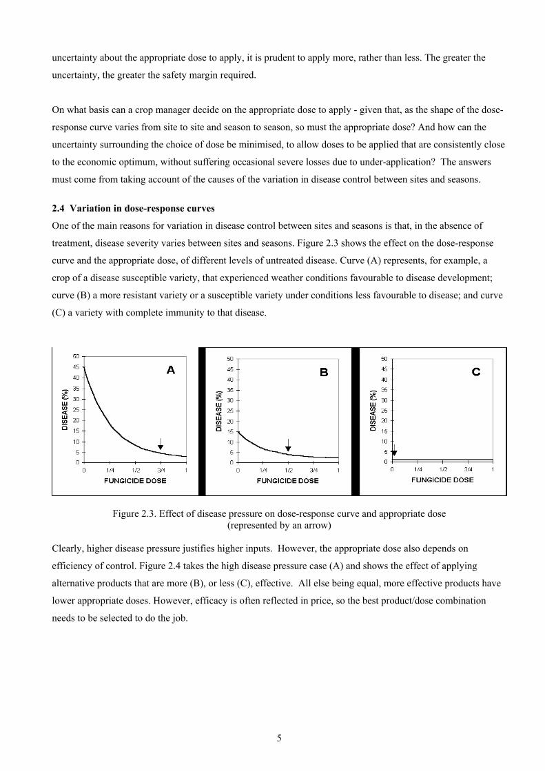
2.4 Variation in dose-response curves
One of the main reasons for variation in disease control between sites and seasons is that, in the absence of
treatment, disease severity varies between sites and seasons. Figure 2.3 shows the effect on the dose-response
curve and the appropriate dose, of different levels of untreated disease. Curve (A) represents, for example, a
crop of a disease susceptible variety, that experienced weather conditions favourable to disease development;
curve (B) a more resistant variety or a susceptible variety under conditions less favourable to disease; and curve
(C) a variety with complete immunity to that disease.
Figure 2.3. Effect of disease pressure on dose-response curve and appropriate dose (represented by an arrow)
Clearly, higher disease pressure justifies higher inputs. However, the appropriate dose also depends on
efficiency of control. Figure 2.4 takes the high disease pressure case (A) and shows the effect of applying
alternative products that are more (B), or less (C), effective. All else being equal, more effective products have
lower appropriate doses. However, efficacy is often reflected in price, so the best product/dose combination
needs to be selected to do the job.

6
Figure 2.4. Effect of fungicide activity on dose-response curves and appropriate dose. It can be seen, from the examples shown above, that the appropriate dose in a range of circumstances can vary
between the recommended dose and zero. A crop manager who is better able to quantify disease pressure and
predict efficiency of control, will be able to apply doses that are consistently closer to the economic optimum.
This will reduce unit cost of production and provide a sound rationale for the dose of pesticide used.

7
3.0 MATERIALS AND METHODS
3.1 Sites
This report covers work conducted over four harvest years at sites selected to target the main foliar diseases of
winter wheat – Septoria tritici, Stagonospora nodorum, yellow rust, brown rust and powdery mildew. The
location of sites and varieties used are listed in Table 3.1.
Table 3.1 Experiment numbers, sites, harvest years, varieties and target diseases
Experiment
number Site
Harvest
year Variety Target disease
1 Pelynt, Looe, Cornwall 2001 Savannah S. nodorum
2 Terrington-St Clement, Norfolk 2001 Brigadier Yellow rust
3 Henley, Ipswich, Suffolk 2001 Equinox Yellow rust
4 Morley, Wymondham, Norfolk 2001 Riband Brown rust/S. tritici
5 Milton, Leuchars, Fife 2001 Consort S. tritici
6 Dunecht, Aberdeenshire 2001 Riband Powdery mildew
7 Pelynt, Looe, Cornwall 2002 Savannah S. nodorum
8 Terrington-St Clement, Norfolk 2002 Brigadier Yellow rust
9 Morley, Wymondham, Norfolk 2002 Brigadier Yellow rust
10 Otley, Suffolk 2002 Shamrock Brown rust
11 Kilrie, Kirkcaldy, Fife 2002 Consort S. tritici
12 Dunecht, Aberdeenshire 2002 Claire Powdery mildew
13 Pelynt, Looe, Cornwall 2003 Savannah S. nodorum
14 Terrington-St Clement, Norfolk 2003 Brigadier Yellow rust
15 Morley, Wymondham, Norfolk 2003 Consort S. tritici
16 Otley, Suffolk 2003 Shamrock Brown rust
17 Coatown of Balgonie, Glenrothes, Fife 2003 Consort S. tritici
18 Dunecht, Alford, Aberdeenshire 2003 Claire Powdery mildew
19 Carlow, Ireland 2003 Madrigal S. tritici
20 Pelynt, Cornwall 2004 Savannah S. nodorum
21 Terrington-St Clement, Norfolk 2004 Brigadier Yellow rust
22 Morley, Wymondham, Norfolk 2004 Consort S. tritici
23 Otley, Suffolk 2004 Shamrock Brown rust
24 Coaltown of Balgonie, Glenrothes, Fife 2004 Consort S. tritici
25 Dunecht, Aberdeenshire 2004 Claire Powdery mildew
26 Carlow, Ireland 2004 Madrigal S. tritici

8
3.2 Site selection and establishment
First wheat sites with at least a one-year break from cereals (excluding oats) were chosen. Soil was sampled for
pH and nutrient analysis and plots were drilled using a suitable plot drill (e.g. Øyjord) at a seed rate appropriate
for the locality and soil type. Plot size was variable to fit in with local farm tramlines, but was in the range of 20
- 60m². All inputs other than fungicides were applied to ensure that the crop remained free from nutritional
deficiencies, or severe pest or weed infestations. At yellow rust sites and some brown rust sites, pots of rust-
infected plants were planted out in a regular grid pattern in the spring to maximise the chance of disease
development.
3.3 Experiment design
A randomised block design incorporating between 33 and 45 treatments with three replicates was used for all
experiments. At sites targeting rusts or mildew, guard plots of a variety resistant to the target disease were
drilled alternately with treatment plots wherever possible.
3.4 Fungicide treatments
Fungicide treatments were applied as single sprays. The target stage for fungicide application was determined
by pathogen development. At the S. tritici sites, the target timing was at the emergence of eventual leaf 2. This
was usually at GS 33, but may have occurred at GS 32 in some crops. Crop development was checked regularly
from the beginning of GS 31 to ensure that the emergence of this leaf was identified correctly. This growth
stage was also the timing for the yellow rust and mildew sites, but at these sites, the timing was adjusted earlier
if early epidemic development required. Brown rust and S. nodorum are characterised by rapid development
late in the season, so the target timing for these sites was at GS 37-39 rather than GS 33 unless there was a risk
of severe disease development at GS 33.
Sprays were applied in 200-300 litres water/ha using hand-held pressurised plot spraying equipment fitted with
flat fan nozzles, selected to produce a medium spray quality at 200-300 kPa pressure. Each fungicide product
was applied at quarter, half, full and double the label recommended dose. Double dose treatments were applied
for specific experimental purposes and must not be applied by farmers to farm crops. . Crop that received double
dose treatments was disposed of safely at harvest.
Details of fungicide treatments at each site in each year are given in Tables 3.2 – 3.14.

9
Table 3.2 Treatments for Experiment 1 (Site 1, 2001)
Treatment code Active ingredient Product Dose product/ha
Standards
1 Epoxiconazole Opus 2.00 litre
2 Epoxiconazole Opus 1.00 litre
3 Epoxiconazole Opus 0.50 litre
4 Epoxiconazole Opus 0.25 litre
5 Azoxystrobin Amistar 2.00 litre 6 Azoxystrobin Amistar 1.00 litre
7 Azoxystrobin Amistar 0.50 litre
8 Azoxystrobin Amistar 0.25 litre
Test actives
9 Trifloxystrobin Twist 4.00 litre
10 Trifloxystrobin Twist 2.00 litre
11 Trifloxystrobin Twist 1.00 litre
12 Trifloxystrobin Twist 0.50 litre
13 Picoxystrobin Acanto 2.00 litre
14 Picoxystrobin Acanto 1.00 litre
15 Picoxystrobin Acanto 0.50 litre
16 Picoxystrobin Acanto 0.25 litre
17 Pyraclostrobin Vivid 2.00 litre
18 Pyraclostrobin Vivid 1.00 litre
19 Pyraclostrobin Vivid 0.50 litre
20 Pyraclostrobin Vivid 0.25 litre
21 Metconazole Caramba 3.00 litre
22 Metconazole Caramba 1.50 litre
23 Metconazole Caramba 0.75 litre
24 Metconazole Caramba 0.375 litre
25 Fluquinconazole Flamenco 2.50 litre
26 Fluquinconazole Flamenco 1.25 litre
27 Fluquinconazole Flamenco 0.625 litre
28 Fluquinconazole Flamenco 0.3125 litre
29 Cyprodinil Unix 2.00 kg
30 Cyprodinil Unix 1.00 kg
31 Cyprodinil Unix 0.5 kg
32 Cyprodinil Unix 0.25 kg
33 Untreated - -
34 Untreated - -

10
Table 3.3 Treatments for Experiments 2, 3, 4 & 5 (Sites 2, 3, 4 & 5, 2001)
Treatment code Active ingredient Product Dose product/ha
Standards
1 Epoxiconazole Opus 2.00 litre
2 Epoxiconazole Opus 1.00 litre
3 Epoxiconazole Opus 0.50 litre
4 Epoxiconazole Opus 0.25 litre
5 Azoxystrobin Amistar 2.00 litre 6 Azoxystrobin Amistar 1.00 litre
7 Azoxystrobin Amistar 0.50 litre
8 Azoxystrobin Amistar 0.25 litre
Test actives
9 Trifloxystrobin Twist 4.00 litre
10 Trifloxystrobin Twist 2.00 litre
11 Trifloxystrobin Twist 1.00 litre
12 Trifloxystrobin Twist 0.50 litre
13 Picoxystrobin Acanto 2.00 litre
14 Picoxystrobin Acanto 1.00 litre
15 Picoxystrobin Acanto 0.50 litre
16 Picoxystrobin Acanto 0.25 litre
17 Pyraclostrobin Vivid 2.00 litre
18 Pyraclostrobin Vivid 1.00 litre
19 Pyraclostrobin Vivid 0.50 litre
20 Pyraclostrobin Vivid 0.25 litre
21 Famoxadone -
22 Famoxadone -
23 Famoxadone -
24 Famoxadone -
25 Metconazole Caramba 3.00 litre
26 Metconazole Caramba 1.50 litre
27 Metconazole Caramba 0.75 litre
28 Metconazole Caramba 0.375 litre
29 Fluquinconazole Flamenco 2.50 litre
30 Fluquinconazole Flamenco 1.25 litre
31 Fluquinconazole Flamenco 0.625 litre
32 Fluquinconazole Flamenco 0.3125 litre
33 Untreated - -
34 Untreated - -

11
Table 3.4 Treatments for Experiment 6 (Site 6, 2001)
Treatment code Active ingredient Product Dose product/ha
Standards
1 Epoxiconazole Opus 2.00 litre
2 Epoxiconazole Opus 1.00 litre
3 Epoxiconazole Opus 0.50 litre
4 Epoxiconazole Opus 0.25 litre
5 Fenpropidin Tern 2.00 litre 6 Fenpropidin Tern 1.00 litre
7 Fenpropidin Tern 0.50 litre
8 Fenpropidin Tern 0.25 litre
Test actives
9 Fluquinconazole Flamenco 2.50 litre
10 Fluquinconazole Flamenco 1.25 litre
11 Fluquinconazole Flamenco 0.625 litre
12 Fluquinconazole Flamenco 0.3125 litre
13 Metconazole Caramba 3.00 litre
14 Metconazole Caramba 1.50 litre
15 Metconazole Caramba 0.75 litre
16 Metconazole Caramba 0.375 litre
17 Spiroxamine Neon 3.00 litre
18 Spiroxamine Neon 1.50 litre
19 Spiroxamine Neon 0.75 litre
20 Spiroxamine Neon 0.375 litre
21 Cyprodinil Unix 2.00 kg
22 Cyprodinil Unix 1.00 kg
23 Cyprodinil Unix 0.5 kg
24 Cyprodinil Unix 0.25 kg
25 Quinoxyfen Fortress 0.60 litre
26 Quinoxyfen Fortress 0.30 litre
27 Quinoxyfen Fortress 0.15 litre
28 Quinoxyfen Fortress 0.075 litre
29
30
31
32
33 Untreated - -
34 Untreated - -
12
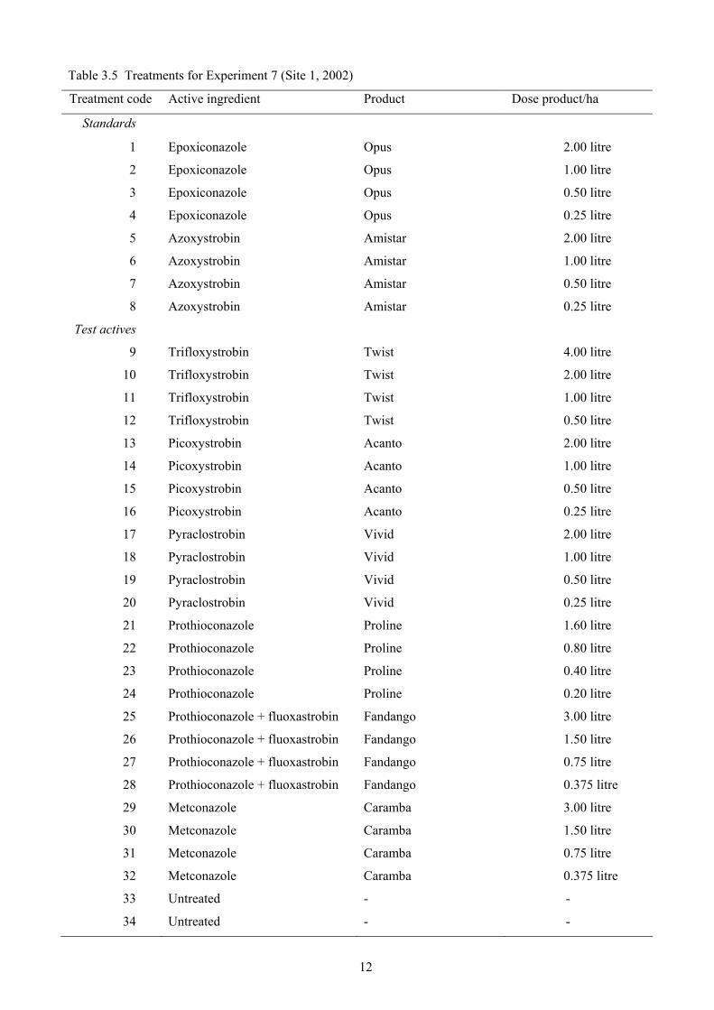
Table 3.5 Treatments for Experiment 7 (Site 1, 2002)
Treatment code Active ingredient Product Dose product/ha
Standards
1 Epoxiconazole Opus 2.00 litre
2 Epoxiconazole Opus 1.00 litre
3 Epoxiconazole Opus 0.50 litre
4 Epoxiconazole Opus 0.25 litre
5 Azoxystrobin Amistar 2.00 litre 6 Azoxystrobin Amistar 1.00 litre
7 Azoxystrobin Amistar 0.50 litre
8 Azoxystrobin Amistar 0.25 litre
Test actives
9 Trifloxystrobin Twist 4.00 litre
10 Trifloxystrobin Twist 2.00 litre
11 Trifloxystrobin Twist 1.00 litre
12 Trifloxystrobin Twist 0.50 litre
13 Picoxystrobin Acanto 2.00 litre
14 Picoxystrobin Acanto 1.00 litre
15 Picoxystrobin Acanto 0.50 litre
16 Picoxystrobin Acanto 0.25 litre
17 Pyraclostrobin Vivid 2.00 litre
18 Pyraclostrobin Vivid 1.00 litre
19 Pyraclostrobin Vivid 0.50 litre
20 Pyraclostrobin Vivid 0.25 litre
21 Prothioconazole Proline 1.60 litre
22 Prothioconazole Proline 0.80 litre
23 Prothioconazole Proline 0.40 litre
24 Prothioconazole Proline 0.20 litre
25 Prothioconazole + fluoxastrobin Fandango 3.00 litre
26 Prothioconazole + fluoxastrobin Fandango 1.50 litre
27 Prothioconazole + fluoxastrobin Fandango 0.75 litre
28 Prothioconazole + fluoxastrobin Fandango 0.375 litre
29 Metconazole Caramba 3.00 litre
30 Metconazole Caramba 1.50 litre
31 Metconazole Caramba 0.75 litre
32 Metconazole Caramba 0.375 litre
33 Untreated - -
34 Untreated - -

13
Table 3.6 Treatments for Experiments 8, 9, 10 & 11 (Sites 2, 3, 4 & 5, 2002)
Treatment code Active ingredient Product Dose product/ha
Standards
1 Epoxiconazole Opus 2.00 litre
2 Epoxiconazole Opus 1.00 litre
3 Epoxiconazole Opus 0.50 litre
4 Epoxiconazole Opus 0.25 litre
5 Azoxystrobin Amistar 2.00 litre 6 Azoxystrobin Amistar 1.00 litre
7 Azoxystrobin Amistar 0.50 litre
8 Azoxystrobin Amistar 0.25 litre
Test actives
9 Trifloxystrobin Twist 4.00 litre
10 Trifloxystrobin Twist 2.00 litre
11 Trifloxystrobin Twist 1.00 litre
12 Trifloxystrobin Twist 0.50 litre
13 Picoxystrobin Acanto 2.00 litre
14 Picoxystrobin Acanto 1.00 litre
15 Picoxystrobin Acanto 0.50 litre
16 Picoxystrobin Acanto 0.25 litre
17 Pyraclostrobin Vivid 2.00 litre
18 Pyraclostrobin Vivid 1.00 litre
19 Pyraclostrobin Vivid 0.50 litre
20 Pyraclostrobin Vivid 0.25 litre
21 Prothioconazole Proline 1.60 litre
22 Prothioconazole Proline 0.80 litre
23 Prothioconazole Proline 0.40 litre
24 Prothioconazole Proline 0.20 litre
25 Prothioconazole + fluoxastrobin Fandango 3.00 litre
26 Prothioconazole + fluoxastrobin Fandango 1.50 litre
27 Prothioconazole + fluoxastrobin Fandango 0.75 litre
28 Prothioconazole + fluoxastrobin Fandango 0.375 litre
29 Fluquinconazole Flamenco 2.50 litre
30 Fluquinconazole Flamenco 1.25 litre
31 Fluquinconazole Flamenco 0.625 litre
32 Fluquinconazole Flamenco 0.3125 litre
33 Untreated - -
34 Untreated - -

14
Table 3.7 Treatments for Experiment 12 (Site 6, 2002)
Treatment code Active ingredient Product Dose product/ha
Standards
1 Epoxiconazole Opus 2.00 litre
2 Epoxiconazole Opus 1.00 litre
3 Epoxiconazole Opus 0.50 litre
4 Epoxiconazole Opus 0.25 litre
5 Fenpropidin Tern 2.00 litre 6 Fenpropidin Tern 1.00 litre
7 Fenpropidin Tern 0.50 litre
8 Fenpropidin Tern 0.25 litre
9 Fenpropimorph Corbel 2.00 litre
10 Fenpropimorph Corbel 1.00 litre
11 Fenpropimorph Corbel 0.50 litre
12 Fenpropimorph Corbel 0.25 litre
Test actives
13 Prothioconazole Proline 1.60 litre
14 Prothioconazole Proline 0.80 litre
15 Prothioconazole Proline 0.40 litre
16 Prothioconazole Proline 0.20 litre
17 Metrafenone + fenpropimorph Flexity + Corbel 1.00+1.08 litre
18 Metrafenone + fenpropimorph Flexity + Corbel 0.50+0.54 litre
19 Metrafenone + fenpropimorph Flexity + Corbel 0.25+0.27 litre
20 Metrafenone + fenpropimorph Flexity + Corbel 0.125+0.135 litre
21 Spiroxamine Neon 3.00 litre
22 Spiroxamine Neon 1.50 litre
23 Spiroxamine Neon 0.75 litre
24 Spiroxamine Neon 0.375 litre
25 Cyprodinil Unix 2.00 kg
26 Cyprodinil Unix 1.00 kg
27 Cyprodinil Unix 0.5 kg
28 Cyprodinil Unix 0.25 kg
29 Quinoxyfen Fortress 0.60 litre
30 Quinoxyfen Fortress 0.30 litre
31 Quinoxyfen Fortress 0.15 litre
32 Quinoxyfen Fortress 0.075 litre
33 Untreated - -
34 Untreated - -

15
Table 3.8 Treatments for Experiment 13 (Site 1, 2003)
Treatment code Active ingredient Product Dose product/ha
Standards
1 Epoxiconazole Opus 2.00 litre
2 Epoxiconazole Opus 1.00 litre
3 Epoxiconazole Opus 0.50 litre
4 Epoxiconazole Opus 0.25 litre
5 Azoxystrobin Amistar 2.00 litre 6 Azoxystrobin Amistar 1.00 litre
7 Azoxystrobin Amistar 0.50 litre
8 Azoxystrobin Amistar 0.25 litre
Test actives
9 Trifloxystrobin Swift 1.00 litre
10 Trifloxystrobin Swift 0.50 litre
11 Trifloxystrobin Swift 0.25 litre
12 Trifloxystrobin Swift 0.125 litre
13 Picoxystrobin Acanto 2.00 litre
14 Picoxystrobin Acanto 1.00 litre
15 Picoxystrobin Acanto 0.50 litre
16 Picoxystrobin Acanto 0.25 litre
17 Pyraclostrobin Vivid 2.00 litre
18 Pyraclostrobin Vivid 1.00 litre
19 Pyraclostrobin Vivid 0.50 litre
20 Pyraclostrobin Vivid 0.25 litre
21 Prothioconazole Proline 1.60 litre
22 Prothioconazole Proline 0.80 litre
23 Prothioconazole Proline 0.40 litre
24 Prothioconazole Proline 0.20 litre
25 Prothioconazole + fluoxastrobin Fandango 3.00 litre
26 Prothioconazole + fluoxastrobin Fandango 1.50 litre
27 Prothioconazole + fluoxastrobin Fandango 0.75 litre
28 Prothioconazole + fluoxastrobin Fandango 0.375 litre
29 Epoxiconazole + dimoxystrobin Swing Gold 3.00 litre
30 Epoxiconazole + dimoxystrobin Swing Gold 1.50 litre
31 Epoxiconazole + dimoxystrobin Swing Gold 0.75 litre
32 Epoxiconazole + dimoxystrobin Swing Gold 0.375 litre
33 Untreated - -
34 Untreated - -

16
Table 3.9 Treatments for Experiments 14, 15, 16, 17 & 19 (Sites 2, 3, 4, 5 & 7, 2003)
Treatment code Active ingredient Product Dose product/ha
Standards
1 Epoxiconazole Opus 2.00 litre
2 Epoxiconazole Opus 1.00 litre
3 Epoxiconazole Opus 0.50 litre
4 Epoxiconazole Opus 0.25 litre
Test actives
Pyraclostrobin + epoxiconazole Vivid + Opus 2.00+2.00 litre
Pyraclostrobin + epoxiconazole Vivid + Opus 1.00+1.00 litre
Pyraclostrobin + epoxiconazole Vivid + Opus 0.50+0.50 litre
Pyraclostrobin + epoxiconazole Vivid + Opus 0.25+0.25 litre
9 Trifloxystrobin Swift 1.00 litre
10 Trifloxystrobin Swift 0.50 litre
11 Trifloxystrobin Swift 0.25 litre
12 Trifloxystrobin Swift 0.125 litre
13 Picoxystrobin Acanto 2.00 litre
14 Picoxystrobin Acanto 1.00 litre
15 Picoxystrobin Acanto 0.50 litre
16 Picoxystrobin Acanto 0.25 litre
17 Pyraclostrobin Vivid 2.00 litre
18 Pyraclostrobin Vivid 1.00 litre
19 Pyraclostrobin Vivid 0.50 litre
20 Pyraclostrobin Vivid 0.25 litre
21 Prothioconazole Proline 1.60 litre
22 Prothioconazole Proline 0.80 litre
23 Prothioconazole Proline 0.40 litre
24 Prothioconazole Proline 0.20 litre
25 Prothioconazole + fluoxastrobin Fandango 3.00 litre
26 Prothioconazole + fluoxastrobin Fandango 1.50 litre
27 Prothioconazole + fluoxastrobin Fandango 0.75 litre
28 Prothioconazole + fluoxastrobin Fandango 0.375 litre
29 Trifloxystrobin + epoxiconazole Swift + Opus 1.00+2.00 litre
30 Trifloxystrobin + epoxiconazole Swift + Opus 0.50+1.00 litre
31 Trifloxystrobin + epoxiconazole Swift + Opus 0.25+0.50 litre
32 Trifloxystrobin + epoxiconazole Swift + Opus 0.125+0.25 litre
33 Untreated - -
34 Untreated - -

17
Table 3.10 Treatments for Experiment 17 (Site 6, 2003)
Treatment code Active ingredient Product Dose product/ha
Standards
1 Epoxiconazole Opus 2.00 litre
2 Epoxiconazole Opus 1.00 litre
3 Epoxiconazole Opus 0.50 litre
4 Epoxiconazole Opus 0.25 litre
5 Fenpropidin Tern 2.00 litre 6 Fenpropidin Tern 1.00 litre
7 Fenpropidin Tern 0.50 litre
8 Fenpropidin Tern 0.25 litre
9 Fenpropimorph Corbel 2.00 litre
10 Fenpropimorph Corbel 1.00 litre
11 Fenpropimorph Corbel 0.50 litre
12 Fenpropimorph Corbel 0.25 litre
Test actives
13 Prothioconazole Proline 1.60 litre
14 Prothioconazole Proline 0.80 litre
15 Prothioconazole Proline 0.40 litre
16 Prothioconazole Proline 0.20 litre
17 Metrafenone + fenpropimorph Flexity + Corbel 1.00+1.08 litre
18 Metrafenone + fenpropimorph Flexity + Corbel 0.50+0.54 litre
19 Metrafenone + fenpropimorph Flexity + Corbel 0.25+0.27 litre
20 Metrafenone + fenpropimorph Flexity + Corbel 0.125+0.135 litre
21 Spiroxamine Neon 3.00 litre
22 Spiroxamine Neon 1.50 litre
23 Spiroxamine Neon 0.75 litre
24 Spiroxamine Neon 0.375 litre
25 Cyprodinil Unix 2.00 kg
26 Cyprodinil Unix 1.00 kg
27 Cyprodinil Unix 0.5 kg
28 Cyprodinil Unix 0.25 kg
29 Quinoxyfen Fortress 0.60 litre
30 Quinoxyfen Fortress 0.30 litre
31 Quinoxyfen Fortress 0.15 litre
32 Quinoxyfen Fortress 0.075 litre
33 Untreated - -
34 Untreated - -

18
Table 3.11 Treatments for Experiment 20 (Site 1, 2004)
Treatment code Active ingredient Product Dose product/ha Standards
1 Epoxiconazole Opus 2.00 litre 2 Epoxiconazole Opus 1.00 litre 3 Epoxiconazole Opus 0.50 litre 4 Epoxiconazole Opus 0.25 litre 5 Chlorothalonil Bravo 4.00 litre 6 Chlorothalonil Bravo 2.00 litre 7 Chlorothalonil Bravo 1.00 litre 8 Chlorothalonil Bravo 0.50 litre
Test actives 9 Pyraclostrobin Vivid 2.00 litre
10 Pyraclostrobin Vivid 1.00 litre 11 Pyraclostrobin Vivid 0.50 litre 12 Pyraclostrobin Vivid 0.25 litre 13 Trifloxystrobin Swift 1.00 litre 14 Trifloxystrobin Swift 0.50 litre 15 Trifloxystrobin Swift 0.25 litre 16 Trifloxystrobin Swift 0.125 litre 17 Famoxadone + flusilazole Charisma 3.00 litres 18 Famoxadone + flusilazole Charisma 1.50 litres 19 Famoxadone + flusilazole Charisma 0.75 litre 20 Famoxadone + flusilazole Charisma 0.375 litre 21 Prothioconazole Proline 1.60 litre 22 Prothioconazole Proline 0.80 litre 23 Prothioconazole Proline 0.40 litre 24 Prothioconazole Proline 0.20 litre 25 Prothioconazole + fluoxastrobin Fandango 3.00 litre 26 Prothioconazole + fluoxastrobin Fandango 1.50 litre 27 Prothioconazole + fluoxastrobin Fandango 0.75 litre 28 Prothioconazole + fluoxastrobin Fandango 0.375 litre 29 Dimoxystrobin + epoxiconazole Swing Gold 3.00 litre 30 Dimoxystrobin + epoxiconazole Swing Gold 1.50 litre 31 Dimoxystrobin + epoxiconazole Swing Gold 0.75 litre 32 Dimoxystrobin + epoxiconazole Swing Gold 0.375 litre 33 Boscalid + epoxiconazole Tracker 3.00 litres 34 Boscalid + epoxiconazole Tracker 1.50 litres 35 Boscalid + epoxiconazole Tracker 0.75 litre 36 Boscalid + epoxiconazole Tracker 0.375 litre 37 HGCA9 Folpan 80WDG 4.00 kg 38 HGCA9 Folpan 80WDG 2.00 kg 39 HGCA9 Folpan 80WDG 1.00 kg 40 HGCA9 Folpan 80WDG 0.50 kg 41 Untreated --- --- 42 Untreated --- ---
19
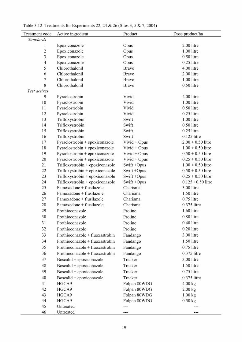
Table 3.12 Treatments for Experiments 22, 24 & 26 (Sites 3, 5 & 7, 2004)
Treatment code Active ingredient Product Dose product/ha Standards
1 Epoxiconazole Opus 2.00 litre 2 Epoxiconazole Opus 1.00 litre 3 Epoxiconazole Opus 0.50 litre 4 Epoxiconazole Opus 0.25 litre 5 Chlorothalonil Bravo 4.00 litre 6 Chlorothalonil Bravo 2.00 litre 7 Chlorothalonil Bravo 1.00 litre 8 Chlorothalonil Bravo 0.50 litre
Test actives 9 Pyraclostrobin Vivid 2.00 litre
10 Pyraclostrobin Vivid 1.00 litre 11 Pyraclostrobin Vivid 0.50 litre 12 Pyraclostrobin Vivid 0.25 litre 13 Trifloxystrobin Swift 1.00 litre 14 Trifloxystrobin Swift 0.50 litre 15 Trifloxystrobin Swift 0.25 litre 16 Trifloxystrobin Swift 0.125 litre 17 Pyraclostrobin + epoxiconazole Vivid + Opus 2.00 + 0.50 litre 18 Pyraclostrobin + epoxiconazole Vivid + Opus 1.00 + 0.50 litre 19 Pyraclostrobin + epoxiconazole Vivid + Opus 0.50 + 0.50 litre 20 Pyraclostrobin + epoxiconazole Vivid + Opus 0.25 + 0.50 litre 21 Trifloxystrobin + epoxiconazole Swift +Opus 1.00 + 0.50 litre 22 Trifloxystrobin + epoxiconazole Swift +Opus 0.50 + 0.50 litre 23 Trifloxystrobin + epoxiconazole Swift +Opus 0.25 + 0.50 litre 24 Trifloxystrobin + epoxiconazole Swift +Opus 0.125 +0.50 litre 25 Famoxadone + flusilazole Charisma 3.00 litre 26 Famoxadone + flusilazole Charisma 1.50 litre 27 Famoxadone + flusilazole Charisma 0.75 litre 28 Famoxadone + flusilazole Charisma 0.375 litre 29 Prothioconazole Proline 1.60 litre 30 Prothioconazole Proline 0.80 litre 31 Prothioconazole Proline 0.40 litre 32 Prothioconazole Proline 0.20 litre 33 Prothioconazole + fluoxastrobin Fandango 3.00 litre 34 Prothioconazole + fluoxastrobin Fandango 1.50 litre 35 Prothioconazole + fluoxastrobin Fandango 0.75 litre 36 Prothioconazole + fluoxastrobin Fandango 0.375 litre 37 Boscalid + epoxiconazole Tracker 3.00 litre 38 Boscalid + epoxiconazole Tracker 1.50 litre 39 Boscalid + epoxiconazole Tracker 0.75 litre 40 Boscalid + epoxiconazole Tracker 0.375 litre 41 HGCA9 Folpan 80WDG 4.00 kg 42 HGCA9 Folpan 80WDG 2.00 kg 43 HGCA9 Folpan 80WDG 1.00 kg 44 HGCA9 Folpan 80WDG 0.50 kg 45 Untreated --- --- 46 Untreated --- ---

20
Table 3.13 Treatments for Experiments 21 & 23 (Sites 2 & 4, 2004)
Treatment code Active ingredient Product Dose product/ha Standards
1 Epoxiconazole Opus 2.00 litre 2 Epoxiconazole Opus 1.00 litre 3 Epoxiconazole Opus 0.50 litre 4 Epoxiconazole Opus 0.25 litre
Test actives 5 Pyraclostrobin Vivid 2.00 litre 6 Pyraclostrobin Vivid 1.00 litre 7 Pyraclostrobin Vivid 0.50 litre 8 Pyraclostrobin Vivid 0.25 litre 9 Trifloxystrobin Swift 1.00 litre
10 Trifloxystrobin Swift 0.50 litre 11 Trifloxystrobin Swift 0.25 litre 12 Trifloxystrobin Swift 0.125 litre 13 Azoxystrobin Amistar 2.00 litre 14 Azoxystrobin Amistar 1.00 litre 15 Azoxystrobin Amistar 0.50 litre 16 Azoxystrobin Amistar 0.25 litre 17 Famoxadone + flusilazole Charisma 3.00 litre 18 Famoxadone + flusilazole Charisma 1.50 litre 19 Famoxadone + flusilazole Charisma 0.75 litre 20 Famoxadone + flusilazole Charisma 0.375 litre 21 Prothioconazole Proline 1.60 litre 22 Prothioconazole Proline 0.80 litre 23 Prothioconazole Proline 0.40 litre 24 Prothioconazole Proline 0.20 litre 25 Prothioconazole + fluoxastrobin Fandango 3.00 litre 26 Prothioconazole + fluoxastrobin Fandango 1.50 litre 27 Prothioconazole + fluoxastrobin Fandango 0.75 litre 28 Prothioconazole + fluoxastrobin Fandango 0.375 litre 29 Boscalid + epoxiconazole Tracker 3.00 litre 30 Boscalid + epoxiconazole Tracker 1.50 litre 31 Boscalid + epoxiconazole Tracker 0.75 litre 32 Boscalid + epoxiconazole Tracker 0.375 litre 33 HGCA9 Folpan 80WDG 4.00 kg 34 HGCA9 Folpan 80WDG 2.00 kg 35 HGCA9 Folpan 80WDG 1.00 kg 36 HGCA9 Folpan 80WDG 0.50 kg 37 Untreated --- --- 38 Untreated --- ---
21
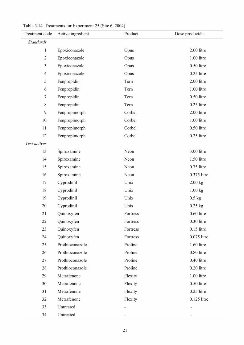
Table 3.14 Treatments for Experiment 25 (Site 6, 2004)
Treatment code Active ingredient Product Dose product/ha
Standards
1 Epoxiconazole Opus 2.00 litre
2 Epoxiconazole Opus 1.00 litre
3 Epoxiconazole Opus 0.50 litre
4 Epoxiconazole Opus 0.25 litre
5 Fenpropidin Tern 2.00 litre 6 Fenpropidin Tern 1.00 litre
7 Fenpropidin Tern 0.50 litre
8 Fenpropidin Tern 0.25 litre
9 Fenpropimorph Corbel 2.00 litre
10 Fenpropimorph Corbel 1.00 litre
11 Fenpropimorph Corbel 0.50 litre
12 Fenpropimorph Corbel 0.25 litre
Test actives
13 Spiroxamine Neon 3.00 litre
14 Spiroxamine Neon 1.50 litre
15 Spiroxamine Neon 0.75 litre
16 Spiroxamine Neon 0.375 litre
17 Cyprodinil Unix 2.00 kg
18 Cyprodinil Unix 1.00 kg
19 Cyprodinil Unix 0.5 kg
20 Cyprodinil Unix 0.25 kg
21 Quinoxyfen Fortress 0.60 litre
22 Quinoxyfen Fortress 0.30 litre
23 Quinoxyfen Fortress 0.15 litre
24 Quinoxyfen Fortress 0.075 litre
25 Prothioconazole Proline 1.60 litre
26 Prothioconazole Proline 0.80 litre
27 Prothioconazole Proline 0.40 litre
28 Prothioconazole Proline 0.20 litre
29 Metrafenone Flexity 1.00 litre
30 Metrafenone Flexity 0.50 litre
31 Metrafenone Flexity 0.25 litre
32 Metrafenone Flexity 0.125 litre
33 Untreated - -
34 Untreated - -
22
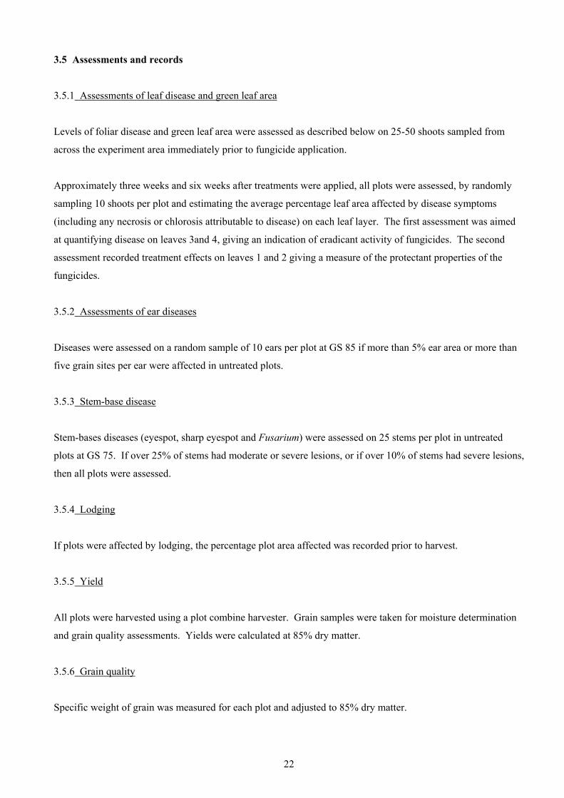
3.5 Assessments and records
3.5.1 Assessments of leaf disease and green leaf area
Levels of foliar disease and green leaf area were assessed as described below on 25-50 shoots sampled from
across the experiment area immediately prior to fungicide application.
Approximately three weeks and six weeks after treatments were applied, all plots were assessed, by randomly
sampling 10 shoots per plot and estimating the average percentage leaf area affected by disease symptoms
(including any necrosis or chlorosis attributable to disease) on each leaf layer. The first assessment was aimed
at quantifying disease on leaves 3and 4, giving an indication of eradicant activity of fungicides. The second
assessment recorded treatment effects on leaves 1 and 2 giving a measure of the protectant properties of the
fungicides.
3.5.2 Assessments of ear diseases
Diseases were assessed on a random sample of 10 ears per plot at GS 85 if more than 5% ear area or more than
five grain sites per ear were affected in untreated plots.
3.5.3 Stem-base disease
Stem-bases diseases (eyespot, sharp eyespot and Fusarium) were assessed on 25 stems per plot in untreated
plots at GS 75. If over 25% of stems had moderate or severe lesions, or if over 10% of stems had severe lesions,
then all plots were assessed.
3.5.4 Lodging
If plots were affected by lodging, the percentage plot area affected was recorded prior to harvest.
3.5.5 Yield
All plots were harvested using a plot combine harvester. Grain samples were taken for moisture determination
and grain quality assessments. Yields were calculated at 85% dry matter.
3.5.6 Grain quality
Specific weight of grain was measured for each plot and adjusted to 85% dry matter.

23
Agronomic records
Details of site, soil type and all agrochemical inputs were recorded.
3.6 Data handling
Disease, green leaf area, yield and grain quality data were collected manually or directly onto portable
computers. All data were transferred to Microsoft Excel worksheets after collection.
3.7 Statistical analysis
3.7.1 Individual season and site assessments
Each season, each assessment (site, variate, date, leaf layer) was summarised by analysis of variance and the
validity of the analysis was checked by examination of residuals. An over-assessment analysis of data from the
previous Appropriate Fungicide Dose project provides a more powerful assessment of the need for transformation
than can be obtained from analysis of a single assessment. Such an analysis has shown that, whilst no
transformation is needed for yield or specific weights, a logit transformation of %disease and %green leaf area
provides a more valid analysis. Thus disease and green leaf area were analysed on a logit scale and back-
transformed for presentation.
A small number of extreme outliers were removed from the data after consultation as to the cause.
In some cases plots of residuals against plot number showed a linear trend in the residuals within some of the
blocks. These trends were removed by using covariates on plot number within each block.
For each disease assessment, dose-response curves were plotted for each fungicide and exponential curves, of the
form y=a+bekx , where y = % disease and x = proportion of the recommended dose were fitted. Exponential
curves were also fitted to the green leaf areas and harvest variables. All curves were constrained to pass through
the mean of the untreated (dose=0) plots.
Variates that did not contribute useful information were excluded from further analysis. These were defined to be
variates for which there was no significant effect of treatment and of differences between products or doses,
disease variates for which there was an average of less than 5% disease on untreated plots, and green leaf areas
for which there was more than an average of 90% green leaf area on the untreated plots. In addition, assessments
where more than one disease was recorded on a particular date were examined to check whether they were
reliable. Any assessments felt to be unsafe were excluded from over-assessment means.
Over-assessment means were calculated for each site and disease, together with corresponding green leaf area
means. Means for all transformed variables were calculated on the logit scale and then back-transformed for
24
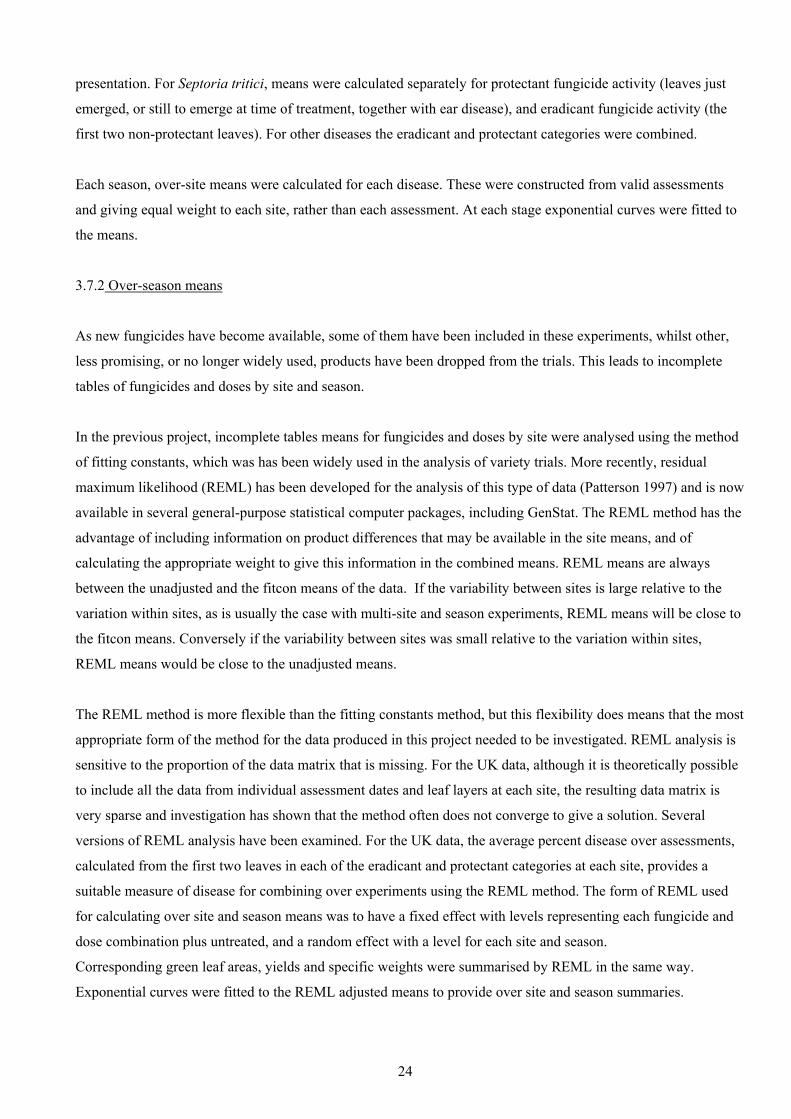
presentation. For Septoria tritici, means were calculated separately for protectant fungicide activity (leaves just
emerged, or still to emerge at time of treatment, together with ear disease), and eradicant fungicide activity (the
first two non-protectant leaves). For other diseases the eradicant and protectant categories were combined.
Each season, over-site means were calculated for each disease. These were constructed from valid assessments
and giving equal weight to each site, rather than each assessment. At each stage exponential curves were fitted to
the means.
3.7.2 Over-season means
As new fungicides have become available, some of them have been included in these experiments, whilst other,
less promising, or no longer widely used, products have been dropped from the trials. This leads to incomplete
tables of fungicides and doses by site and season.
In the previous project, incomplete tables means for fungicides and doses by site were analysed using the method
of fitting constants, which was has been widely used in the analysis of variety trials. More recently, residual
maximum likelihood (REML) has been developed for the analysis of this type of data (Patterson 1997) and is now
available in several general-purpose statistical computer packages, including GenStat. The REML method has the
advantage of including information on product differences that may be available in the site means, and of
calculating the appropriate weight to give this information in the combined means. REML means are always
between the unadjusted and the fitcon means of the data. If the variability between sites is large relative to the
variation within sites, as is usually the case with multi-site and season experiments, REML means will be close to
the fitcon means. Conversely if the variability between sites was small relative to the variation within sites,
REML means would be close to the unadjusted means.
The REML method is more flexible than the fitting constants method, but this flexibility does means that the most
appropriate form of the method for the data produced in this project needed to be investigated. REML analysis is
sensitive to the proportion of the data matrix that is missing. For the UK data, although it is theoretically possible
to include all the data from individual assessment dates and leaf layers at each site, the resulting data matrix is
very sparse and investigation has shown that the method often does not converge to give a solution. Several
versions of REML analysis have been examined. For the UK data, the average percent disease over assessments,
calculated from the first two leaves in each of the eradicant and protectant categories at each site, provides a
suitable measure of disease for combining over experiments using the REML method. The form of REML used
for calculating over site and season means was to have a fixed effect with levels representing each fungicide and
dose combination plus untreated, and a random effect with a level for each site and season.
Corresponding green leaf areas, yields and specific weights were summarised by REML in the same way.
Exponential curves were fitted to the REML adjusted means to provide over site and season summaries.

25
4.0 RESULTS
4.1 Stagonospora nodorum experiments
4.1.1 Disease control.
All currently available commercial varieties that are susceptible to S. nodorum are also susceptible to Septoria
tritici. Since both diseases are favoured by similar weather conditions, mixed infections frequently occur. It is
rarely possible to differentiate in the field between the foliar symptoms caused by the two fungi and activity of
fungicides against S. nodorum can therefore best be assessed by the ear symptoms known as glume blotch.
Figure 4.1 shows the dose response curves fitted from parameters given in Table 4.1 derived from data from the
2001 site (Experiment 1). A prolonged dry spell during May 2001 limited the development of disease on upper
leaves. Control of glume blotch from fungicides applied, as in this case, on 18 May, well before ear emergence,
largely reflects the fungicides’ ability to protect the upper leaves from infection from where inoculum could be
spread to the ears when wet weather returned during June. All fungicides showed activity against S. nodorum,
most azoles required between a half and full dose to achieve maximum control. The control of glume blotch
given by Flamenco, however, did not increase above quarter dose. All strobilurin fungicides reduced glume
blotch. The greatest reduction was given by Acanto at high doses but Amistar, Twist and Vivid gave good
control at between half and quarter dose.
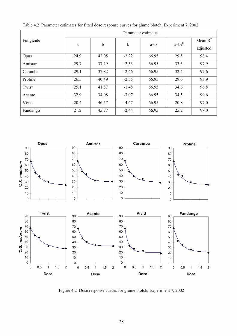
Wet weather during May 2002 delayed spray application until 31 May (GS 49), a week after flag leaf
emergence. As a consequence, a severe epidemic of glume blotch developed. Fungicide performance largely
reflects eradicant activity on the flag leaf with the possibility of some protection of the ear. Again, all
fungicides gave some control of glume blotch, but most required a full dose to give reasonable control. The
exception was Vivid, which at half dose gave a level of control that was equivalent to, or better than, a full dose
of most other fungicides tested (Figure 4.2).
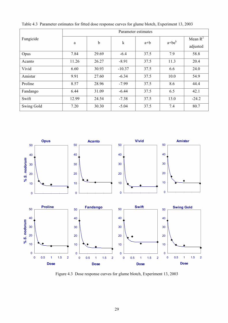
A moderate epidemic of S. nodorum developed in 2003. Spray timing coincided with the emergence of Leaf 2
(9 May) and therefore the control of glume blotch reflects the protectant activity of fungicides (Table 4.3 and
Figure 4.3). All products show low (more negative) k values and achieve maximum control of glume blotch at
between half and full dose. The two azole fungicides (Opus and Proline) gave similar control. Vivid remained
the most active of the strobilurin products and Swift (Twist SC) the least active. Azole/strobilurin mixtures
(Fandango and Swing Gold) showed a small improvement in disease control over the corresponding azole.
Glume blotch did not develop to any great extent at the Cornish site in 2004, possibly due to a severe epidemic
of S. tritici causing competition for infection sites on the upper leaves. Fungicides were applied on 10 May
when leaf 2 was just fully emerged, so disease control was due mainly to the protectant activity of products.

26
With low disease levels, it would be wrong to try to draw too many conclusions about fungicide activity.
However, Charisma, a azole/strobilurin mixture gave poor control relative to other azole/strobilurin mixtures.
Bravo, brought back into the experiment in 2004 because of increased popularity following concerns over S.
tritici resistance to strobilurin fungicides, proved to be a reasonable protectant option for S. nodorum control.
HGCA9, which was also a protectant fungicide was less effective (Table 4.4 and Figure 4.4).

27
Table 4.1 Parameter estimates for fitted dose response curves for glume blotch, Experiment 1, 2001
Parameter estimates
Fungicide a b k a+b a+bek
Mean R2
adjusted
Opus 12.28 5.81 -3.11 18.09 12.54 95.5
Amistar 12.20 5.89 -5.32 18.09 12.23 76.2
Twist 12.37 5.72 -4.62 18.09 12.43 90.6
Acanto 10.87 8.10 -2.23 18.09 10.87 95.1
Vivid 12.91 5.18 -16.63 18.09 12.91 53.4
Proline 14.46 3.98 -4.42 18.09 14.46 8.7
Caramba 13.58 4.67 -3.43 18.09 13.58 95.6
Flamenco 14.15 3.95 -20 18.09 14.15 50.1
Figure 4.1 Dose-response curves for glume blotch, Experiment 1, 2001
Opus
0
5
10
15
20
Sept
oria
nod
orum
(%)
Caramba
0
5
10
15
20
0 0.5 1 1.5 2
Dose
Sept
oria
nod
orum
(%)
Amistar
0
5
10
15
20Twist
0
5
10
15
20
Flamenco
0
5
10
15
20
0 0.5 1 1.5 2
Dose
Acanto
0
5
10
15
20
0 0.5 1 1.5 2
Dose
Vivid
0
5
10
15
20
Proline
0
5
10
15
20
0 0.5 1 1.5 2
Dose
28
Table 4.2 Parameter estimates for fitted dose response curves for glume blotch, Experiment 7, 2002
Parameter estimates
Fungicide a b k a+b a+bek
Mean R2
adjusted
Opus 24.9 42.05 -2.22 66.95 29.5 98.4
Amistar 29.7 37.29 -2.33 66.95 33.3 97.9
Caramba 29.1 37.82 -2.46 66.95 32.4 97.6
Proline 26.5 40.49 -2.55 66.95 29.6 93.9
Twist 25.1 41.87 -1.48 66.95 34.6 96.8
Acanto 32.9 34.08 -3.07 66.95 34.5 99.6
Vivid 20.4 46.57 -4.67 66.95 20.8 97.0
Fandango 21.2 45.77 -2.44 66.95 25.2 98.0
Figure 4.2 Dose response curves for glume blotch, Experiment 7, 2002
Proline
0
10
20
30
40
50
60
70
80
90
Fandango
01020
30405060
708090
0 0.5 1 1.5 2
Dose
Opus
0
10
20
30
40
50
60
70
80
90
% S
. nod
orum
Twist
0102030405060708090
0 0.5 1 1.5 2
Dose
% S
. nod
orum
Amistar
0
10
20
30
40
50
60
70
80
90Caramba
0
10
20
30
40
50
60
70
80
90
Acanto
0102030405060708090
0 0.5 1 1.5 2
Dose
Vivid
0102030405060708090
0 0.5 1 1.5 2
Dose
29
Table 4.3 Parameter estimates for fitted dose response curves for glume blotch, Experiment 13, 2003
Parameter estimates
Fungicide a b k a+b a+bek
Mean R2
adjusted
Opus 7.84 29.69 -6.4 37.5 7.9 58.8
Acanto 11.26 26.27 -8.91 37.5 11.3 20.4
Vivid 6.60 30.93 -10.37 37.5 6.6 24.0
Amistar 9.91 27.60 -6.34 37.5 10.0 54.9
Proline 8.57 28.96 -7.99 37.5 8.6 44.4
Fandango 6.44 31.09 -6.44 37.5 6.5 42.1
Swift 12.99 24.54 -7.38 37.5 13.0 -24.2
Swing Gold 7.20 30.30 -5.04 37.5 7.4 80.7
Figure 4.3 Dose response curves for glume blotch, Experiment 13, 2003
Opus
0
10
20
30
40
50
% S
. nod
orum
Proline
0
10
20
30
40
50
0 0.5 1 1.5 2
Dose
% S
. nod
orum
Acanto
0
10
20
30
40
50Vivid
0
10
20
30
40
50
Fandango
0
10
20
30
40
50
0 0.5 1 1.5 2
Dose
Swift
0
10
20
30
40
50
0 0.5 1 1.5 2
Dose
Amistar
0
10
20
30
40
50
Swing Gold
0
10
20
30
40
50
0 0.5 1 1.5 2
Dose

30
Table 4.4 Parameter estimates for fitted dose response curves for glume blotch, Experiment 20, 2004
Parameter estimates
Fungicide a b k a+b a+bek
Mean R2
adjusted
Opus 6.3 4.6 -2.6 10.8 6.6 95.2
Swing Gold 5.8 5.0 -4.7 10.8 5.9 93.9
Tracker 5.0 5.9 -5.4 10.8 5.0 99.3
Bravo 6.5 4.4 -4.9 10.8 6.5 89.2
HGCA9 7.8 3.0 -16.0 10.8 7.8 66.7
Proline 6.5 4.4 -5.3 10.8 6.5 96.3
Fandango 6.2 4.7 -12.4 10.8 6.2 95.1
Charisma 8.0 2.9 -6.0 10.8 8.0 87.0
Vivid 6.8 4.0 -7.9 10.8 6.8 95.3
Swift 7.4 3.4 -11.4 10.8 7.4 96.7
Figure 4.4 Dose response curves for glume blotch, Experiment 20, 2004
Opus
0
5
10
% S
. nod
orum
Proline
0
5
10
0 0.5 1 1.5 2
Dose
% S
. nod
orum
Swing Gold
0
5
10
Tracker
0
5
10
Fandango
0
5
10
0 0.5 1 1.5 2
Dose
Charisma
0
5
10
0 0.5 1 1.5 2
Dose
Bravo
0
5
10
HGCA9
0
5
10
Vivid
0
5
10
0 0.5 1 1.5 2
Dose
Swift
0
5
10
0 0.5 1 1.5 2
Dose

31
4.1.2 Green leaf area
Because leaves were usually affected by a mixture of S. nodorum and S. tritici, green leaf area assessments
usually reflect the damage done by a combination of the two diseases. However, leaf 4 was primarily affected
by S. nodorum at the early assessment in 2001, and this leaf has been used to give an indication of how the
fungicides affected green leaf area at that site.
The effects of fungicides on the green leaf area on leaf 4 are an indication of their ability to eradicate disease
present at the time of spraying, some three weeks after that leaf emerged. All of the strobilurin fungicides,
except Amistar, maintained green leaf area well. Opus was the most effective azole, giving good levels of green
leaf area, even at half dose. Flamenco and Caramba were considerably less effective, suggesting that their
eradicant activity was being stretched too far, even at full dose (Table 4.5 and Figure 4.5)

32
Table 4.5 Parameter estimates for fitted dose response curves for green leaf area (leaf 4), Experiment 1, 2001
Parameter estimates
Fungicide a b k a+b a+bek
Mean R2
adjusted
Opus 54.6 -46.3 -3.29 8.3 52.9 89.1
Amistar 30.0 -21.7 -1.03 8.3 22.3 56.3
Twist 56.3 -48.0 -2.67 8.3 53.0 78.6
Acanto 77.7 -69.4 -0.91 8.3 49.8 86.3
Vivid 68.4 -60.1 -2.40 8.3 63.0 82.3
Proline -80.7 89.0 0.21 8.3 28.8 82.8
Caramba 88.0 -79.7 -0.34 8.3 31.4 98.6
Flamenco -105.1 113.4 0.09 8.3 19.5 92.3
Figure 4.5 Dose response curves for green leaf area (leaf 4), Experiment 1, 2001
Opus
0
10
20
30
40
50
60
70
80
90
% g
reen
leaf
are
a
Vivid
0102030405060708090
0 0.5 1 1.5 2
Dose
% g
reen
leaf
are
a
Amistar
0
10
20
30
40
50
60
70
80
90Twist
0
10
20
30
40
50
60
70
80
90
Proline
0102030405060708090
0 0.5 1 1.5 2
Dose
Caramba
0102030405060708090
0 0.5 1 1.5 2
Dose
Acanto
0
10
20
30
40
50
60
70
80
90
Flamenco
0102030405060708090
0 0.5 1 1.5 2
Dose
33
4.1.3 Yield
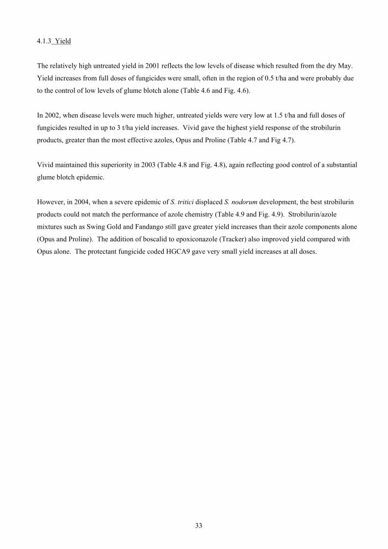
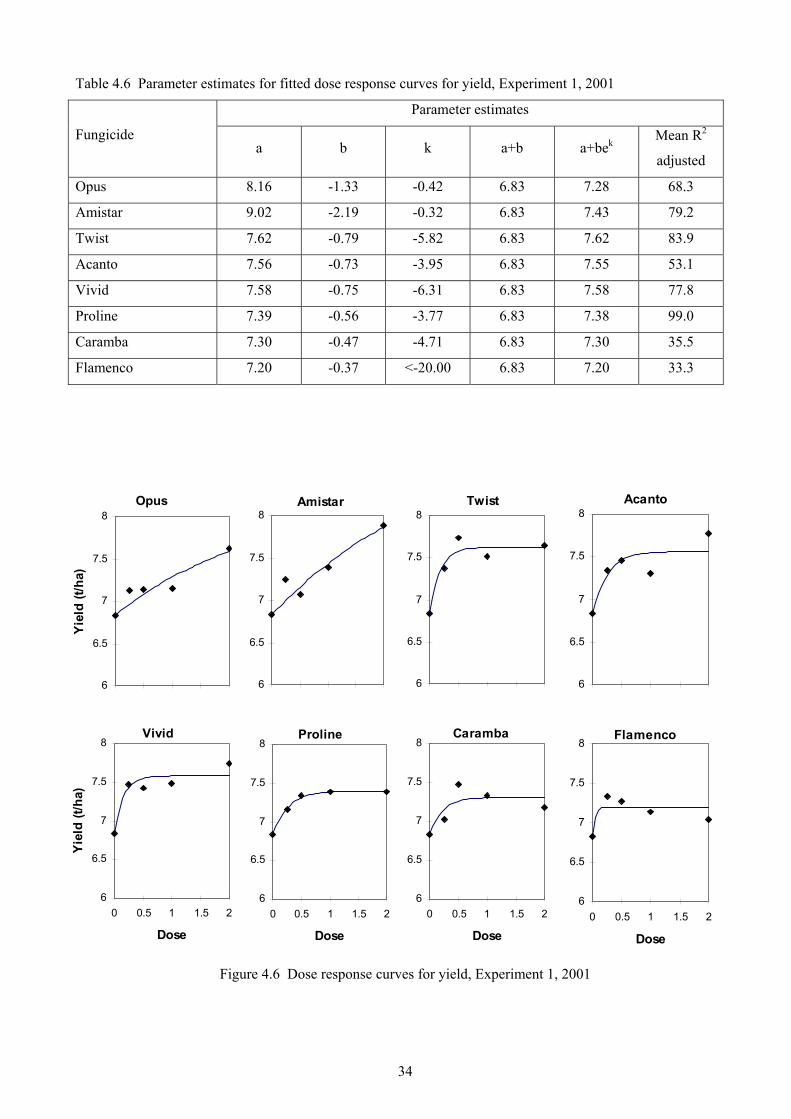
The relatively high untreated yield in 2001 reflects the low levels of disease which resulted from the dry May.
Yield increases from full doses of fungicides were small, often in the region of 0.5 t/ha and were probably due
to the control of low levels of glume blotch alone (Table 4.6 and Fig. 4.6).
In 2002, when disease levels were much higher, untreated yields were very low at 1.5 t/ha and full doses of
fungicides resulted in up to 3 t/ha yield increases. Vivid gave the highest yield response of the strobilurin
products, greater than the most effective azoles, Opus and Proline (Table 4.7 and Fig 4.7).
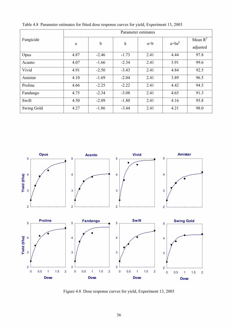
Vivid maintained this superiority in 2003 (Table 4.8 and Fig. 4.8), again reflecting good control of a substantial
glume blotch epidemic.
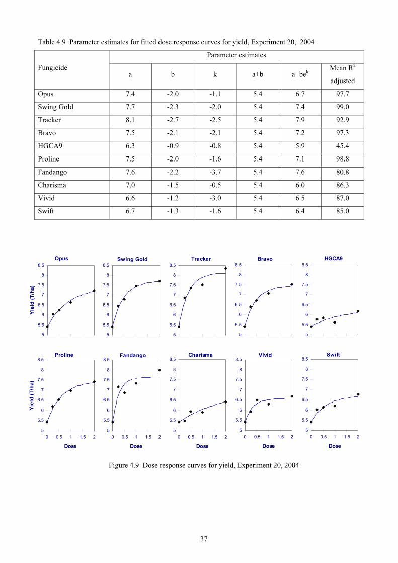
However, in 2004, when a severe epidemic of S. tritici displaced S. nodorum development, the best strobilurin
products could not match the performance of azole chemistry (Table 4.9 and Fig. 4.9). Strobilurin/azole
mixtures such as Swing Gold and Fandango still gave greater yield increases than their azole components alone
(Opus and Proline). The addition of boscalid to epoxiconazole (Tracker) also improved yield compared with
Opus alone. The protectant fungicide coded HGCA9 gave very small yield increases at all doses.
34
Opus
6
6.5
7
7.5
8
Yie
ld (t
/ha)
Vivid
6
6.5
7
7.5
8
0 0.5 1 1.5 2
Dose
Yie
ld (t
/ha)
Amistar
6
6.5
7
7.5
8Twist
6
6.5
7
7.5
8
Proline
6
6.5
7
7.5
8
0 0.5 1 1.5 2
Dose
Caramba
6
6.5
7
7.5
8
0 0.5 1 1.5 2
Dose
Acanto
6
6.5
7
7.5
8
Flamenco
6
6.5
7
7.5
8
0 0.5 1 1.5 2
Dose
Table 4.6 Parameter estimates for fitted dose response curves for yield, Experiment 1, 2001
Parameter estimates
Fungicide a b k a+b a+bek
Mean R2
adjusted
Opus 8.16 -1.33 -0.42 6.83 7.28 68.3
Amistar 9.02 -2.19 -0.32 6.83 7.43 79.2
Twist 7.62 -0.79 -5.82 6.83 7.62 83.9
Acanto 7.56 -0.73 -3.95 6.83 7.55 53.1
Vivid 7.58 -0.75 -6.31 6.83 7.58 77.8
Proline 7.39 -0.56 -3.77 6.83 7.38 99.0
Caramba 7.30 -0.47 -4.71 6.83 7.30 35.5
Flamenco 7.20 -0.37 <-20.00 6.83 7.20 33.3
Figure 4.6 Dose response curves for yield, Experiment 1, 2001

35
Table 4.7 Parameter estimates for fitted dose response curves for yield, Experiment 7, 2002
Parameter estimates
Fungicide a b k a+b a+bek
Mean R2
adjusted
Opus 5.46 -3.97 -0.76 1.49 3.60 93.9
Amistar 3.73 -2.24 -1.32 1.49 3.13 90.9
Caramba 3.57 -2.08 -1.47 1.49 3.09 95.4
Proline 5.57 -4.08 -0.76 1.49 3.65 99.5
Twist 4.09 -2.60 -1.02 1.49 3.16 98.9
Acanto 3.39 -1.90 -1.59 1.49 3.01 99.2
Vivid 5.61 -4.12 -1.95 1.49 5.02 98.7
Fandango 4.59 -3.10 -1.31 1.49 3.76 97.6
Figure 4.7 Dose response curves for yield, Experiment 7, 2002
Opus
1
2
3
4
5
6
Yie
ld (t
/ha)
Twist
1
2
3
4
5
6
0 0.5 1 1.5 2
Dose
Yie
ld (t
/ha)
Amistar
1
2
3
4
5
6Caramba
1
2
3
4
5
6
Acanto
1
2
3
4
5
6
0 0.5 1 1.5 2
Dose
Vivid
1
2
3
4
5
6
0 0.5 1 1.5 2
Dose
Proline
1
2
3
4
5
6
Fandango
1
2
3
4
5
6
0 0.5 1 1.5 2
Dose
36
Table 4.8 Parameter estimates for fitted dose response curves for yield, Experiment 13, 2003
Parameter estimates
Fungicide a b k a+b a+bek
Mean R2
adjusted
Opus 4.87 -2.46 -1.73 2.41 4.44 97.8
Acanto 4.07 -1.66 -2.34 2.41 3.91 99.6
Vivid 4.91 -2.50 -3.43 2.41 4.84 92.5
Amistar 4.10 -1.69 -2.04 2.41 3.89 96.5
Proline 4.66 -2.25 -2.22 2.41 4.42 94.5
Fandango 4.75 -2.34 -3.08 2.41 4.65 91.3
Swift 4.50 -2.09 -1.80 2.41 4.16 95.8
Swing Gold 4.27 -1.86 -3.44 2.41 4.21 98.0
Figure 4.8 Dose response curves for yield, Experiment 13, 2003
Amistar
2
3
4
5
Swing Gold
2
3
4
5
0 0.5 1 1.5 2
Dose
Opus
2
3
4
5
Yie
ld (t
/ha)
Proline
2
3
4
5
0 0.5 1 1.5 2
Dose
Yie
ld (t
/ha)
Acanto
2
3
4
5Vivid
2
3
4
5
Fandango
2
3
4
5
0 0.5 1 1.5 2
Dose
Swift
2
3
4
5
0 0.5 1 1.5 2
Dose
37
Table 4.9 Parameter estimates for fitted dose response curves for yield, Experiment 20, 2004
Parameter estimates
Fungicide a b k a+b a+bek
Mean R2
adjusted
Opus 7.4 -2.0 -1.1 5.4 6.7 97.7
Swing Gold 7.7 -2.3 -2.0 5.4 7.4 99.0
Tracker 8.1 -2.7 -2.5 5.4 7.9 92.9
Bravo 7.5 -2.1 -2.1 5.4 7.2 97.3
HGCA9 6.3 -0.9 -0.8 5.4 5.9 45.4
Proline 7.5 -2.0 -1.6 5.4 7.1 98.8
Fandango 7.6 -2.2 -3.7 5.4 7.6 80.8
Charisma 7.0 -1.5 -0.5 5.4 6.0 86.3
Vivid 6.6 -1.2 -3.0 5.4 6.5 87.0
Swift 6.7 -1.3 -1.6 5.4 6.4 85.0
Figure 4.9 Dose response curves for yield, Experiment 20, 2004
Opus
5
5.5
6
6.5
7
7.5
8
8.5
Yiel
d (T
/ha)
Proline
5
5.5
6
6.5
7
7.5
8
8.5
0 0.5 1 1.5 2
Dose
Yie
ld (T
/ha)
Swing Gold
5
5.5
6
6.5
7
7.5
8
8.5Tracker
5
5.5
6
6.5
7
7.5
8
8.5
Fandango
5
5.5
6
6.5
7
7.5
8
8.5
0 0.5 1 1.5 2
Dose
Charisma
5
5.5
6
6.5
7
7.5
8
8.5
0 0.5 1 1.5 2
Dose
Bravo
5
5.5
6
6.5
7
7.5
8
8.5HGCA9
5
5.5
6
6.5
7
7.5
8
8.5
Vivid
5
5.5
6
6.5
7
7.5
8
8.5
0 0.5 1 1.5 2
Dose
Swift
5
5.5
6
6.5
7
7.5
8
8.5
0 0.5 1 1.5 2
Dose

38
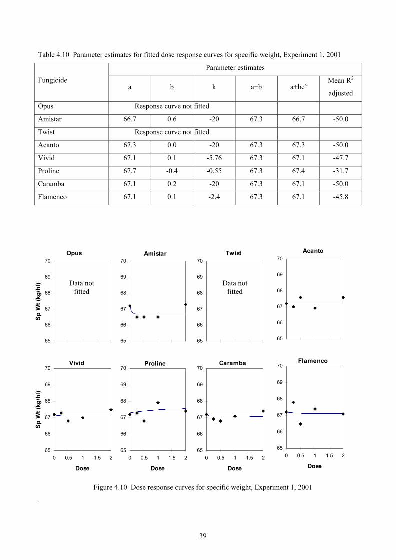
4.1.4 Specific weight
Specific weight of grain was not significantly affected by fungicide treatments at the S. nodorum site in the low
disease year 2001, and for some products it was not possible to fit curves to the data (Table 4.10 and Figure
4.10).
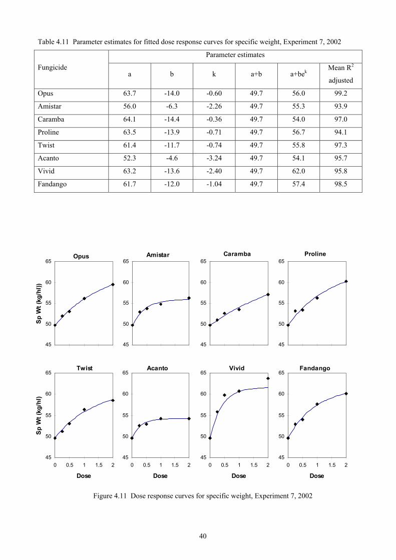
Poor specific weights in untreated plots were increased substantially by fungicide treatments in 2002 as a result
of the control of severe glume blotch (Table 4.11 and Figure 4.11). The effect of different products on specific
weights was in line with their effect on yield.
The shapes of the dose-response curves for specific weights in 2003 (Figure 4.12) were similar to those obtained
for yield. Fandango gave greater specific weights than Proline at quarter dose and half dose, but not at full dose.
Vivid was the most effective strobilurin product at increasing specific weight, equivalent to Opus.
In 2004, the improvement shown by Tracker over straight epoxiconazole in yield was also evident in specific
weights (Table 4.13 and Figure 4.13). Specific weight was not increased by Swift beyond a quarter dose. The
fitted curves for Fandango and Swing Gold were flat beyond a half dose.
39
Table 4.10 Parameter estimates for fitted dose response curves for specific weight, Experiment 1, 2001
Parameter estimates
Fungicide a b k a+b a+bek
Mean R2
adjusted
Opus Response curve not fitted
Amistar 66.7 0.6 -20 67.3 66.7 -50.0
Twist Response curve not fitted
Acanto 67.3 0.0 -20 67.3 67.3 -50.0
Vivid 67.1 0.1 -5.76 67.3 67.1 -47.7
Proline 67.7 -0.4 -0.55 67.3 67.4 -31.7
Caramba 67.1 0.2 -20 67.3 67.1 -50.0
Flamenco 67.1 0.1 -2.4 67.3 67.1 -45.8
Figure 4.10 Dose response curves for specific weight, Experiment 1, 2001
.
Opus
65
66
67
68
69
70
Sp W
t (kg
/hl)
Vivid
65
66
67
68
69
70
0 0.5 1 1.5 2
Dose
Sp W
t (kg
/hl)
Amistar
65
66
67
68
69
70Twist
65
66
67
68
69
70
Proline
65
66
67
68
69
70
0 0.5 1 1.5 2
Dose
Caramba
65
66
67
68
69
70
0 0.5 1 1.5 2
Dose
Acanto
65
66
67
68
69
70
Flamenco
65
66
67
68
69
70
0 0.5 1 1.5 2
Dose
Data not fitted
Data not fitted
40
Table 4.11 Parameter estimates for fitted dose response curves for specific weight, Experiment 7, 2002
Parameter estimates
Fungicide a b k a+b a+bek
Mean R2
adjusted
Opus 63.7 -14.0 -0.60 49.7 56.0 99.2
Amistar 56.0 -6.3 -2.26 49.7 55.3 93.9
Caramba 64.1 -14.4 -0.36 49.7 54.0 97.0
Proline 63.5 -13.9 -0.71 49.7 56.7 94.1
Twist 61.4 -11.7 -0.74 49.7 55.8 97.3
Acanto 52.3 -4.6 -3.24 49.7 54.1 95.7
Vivid 63.2 -13.6 -2.40 49.7 62.0 95.8
Fandango 61.7 -12.0 -1.04 49.7 57.4 98.5
Figure 4.11 Dose response curves for specific weight, Experiment 7, 2002
Opus
45
50
55
60
65
Sp
Wt (
kg/h
l))
Twist
45
50
55
60
65
0 0.5 1 1.5 2
Dose
Sp
Wt (
kg/h
l)
Amistar
45
50
55
60
65Caramba
45
50
55
60
65
Acanto
45
50
55
60
65
0 0.5 1 1.5 2
Dose
Vivid
45
50
55
60
65
0 0.5 1 1.5 2
Dose
Proline
45
50
55
60
65
Fandango
45
50
55
60
65
0 0.5 1 1.5 2
Dose

41
Table 4.12 Parameter estimates for fitted dose response curves for specific weight, Experiment 13, 2003
Parameter estimates
Fungicide a b k a+b a+bek
Mean R2
adjusted
Opus 70.7 -4.80 -2.59 65.9 70.4 99.5
Acanto 69.5 -3.57 -1.98 65.9 69.0 73.6
Vivid 70.9 -4.95 -3.09 65.9 70.7 97.3
Amistar 69.8 -3.90 -1.73 65.9 69.1 82.6
Proline 71.2 -5.31 -2.24 65.9 70.7 94.2
Fandango 70.5 -4.56 -4.21 65.9 70.4 99.6
Swift 69.9 -4.01 -2.24 65.9 69.5 91.6
Swing Gold 69.7 -3.80 -3.86 65.9 69.7 99.7
Figure 4.12 Dose response curves for specific weight, Experiment 13, 2003
Opus
65
66
67
68
69
70
71
72
Sp
Wt (
kg/h
l)
Proline
65
66
67
68
69
70
71
72
0 0.5 1 1.5 2
Dose
Sp
Wt (
kg/h
l)
Acanto
65
66
67
68
69
70
71
72Vivid
65
66
67
68
69
70
71
72
Fandango
65
66
67
68
69
70
71
72
0 0.5 1 1.5 2
Dose
Swift
65
66
67
68
69
70
71
72
0 0.5 1 1.5 2
Dose
Amistar
65
66
67
68
69
70
71
72
Swing Gold
65
66
67
68
69
70
71
72
0 0.5 1 1.5 2
Dose

42
Table 4.13 Parameter estimates for fitted dose response curves for specific weight, Experiment 20, 2004
Parameter estimates
Fungicide a b k a+b a+bek
Mean R2
adjusted
Opus 69.0 -6.2 -0.8 62.8 66.1 94.1
Swing Gold 68.0 -5.2 -6.1 62.8 67.9 94.2
Tracker 69.3 -6.6 -3.1 62.8 69.0 96.6
Bravo 67.4 -4.6 -3.2 62.8 67.2 89.8
HGCA9 66.1 -3.4 -1.0 62.8 64.9 48.2
Proline 67.7 -5.0 -2.0 62.8 67.0 98.0
Fandango 68.0 -5.3 -8.7 62.8 68.0 94.6
Charisma 66.5 -3.8 -1.7 62.8 65.8 76.0
Vivid 68.2 -5.5 -1.0 62.8 66.2 89.4
Swift 66.2 -3.4 -16.0 62.8 66.2 88.0
Figure 4.13 Dose response curves for specific weight, Experiment 20, 2004
Opus
62
63
64
65
66
67
68
69
70
Sp W
t (kg
/hl)
Proline
62
63
64
65
66
67
68
69
70
0 0.5 1 1.5 2
Dose
Sp W
t (kg
/hl)
Swing Gold
62
63
64
65
66
67
68
69
70Tracker
62
63
64
65
66
67
68
69
70
Fandango
62
63
64
65
66
67
68
69
70
0 0.5 1 1.5 2
Dose
Charisma
62
63
64
65
66
67
68
69
70
0 0.5 1 1.5 2
Dose
Bravo
62
63
64
65
66
67
68
69
70HGCA9
62
63
64
65
66
67
68
69
70
Vivid
62
63
64
65
66
67
68
69
70
0 0.5 1 1.5 2
Dose
Swift
62
63
64
65
66
67
68
69
70
0 0.5 1 1.5 2
Dose
43
4.2 Yellow rust experiments
4.2.1 Disease control
With the exception of Experiment 4 in 2001, which was conducted on Equinox, all yellow rust experiments used
the very susceptible variety Brigadier. Occasionally, when weather conditions favoured epidemics of both S.
tritici and yellow rust, the effect of fungicides on yellow rust alone was difficult to assess, particularly late in the
season. Where possible, protectant and eradicant activity of fungicides has been separated.
Parameter estimates for protectant activity of fungicides against yellow rust in 2001 are given in Table 4.14.
and the fitted dose-response curves are shown in Fig. 4.14. Although the levels of yellow rust are low, the
curves suggest that Opus, Proline, Amistar and Acanto all provide very good control of yellow rust, at
quarter/half dose, when applied as protectant sprays.
In 2002, yellow rust data were obtained from two sites, Terrington and Morley. Pooled data from both sites
have been analysed to provide information on protectant and eradicant activity of fungicides. Parameter
estimates and fitted dose-response curves are shown in Table 4.15 and Fig. 4.15 for protectant sprays and in
Table 4.16 and Fig 4.16 for eradicant applications. Individual fungicide products behaved similarly in
protectant and eradicant situations. Opus was very effective, giving good control at a quarter dose. Other azole
products were slightly less effective. Prothioconazole (Proline) was slightly improved by the addition of
fluoxastrobin (Fandango) and Flamenco was the least active of the azoles tested. Vivid was the most active of
the strobilurin products and at half dose gave as good control of yellow rust as full doses of other strobilurins.
Data for protectant and eradicant situations were combined in 2003 and are presented in Table 4.17 and Fig.
4.17. Opus remained slightly more effective than Proline. Vivid appeared to be slightly less effective than in
previous years, but it remained the most effective strobilurin fungicide. Strobilurin/azole mixtures were also
very effective in controlling yellow rust.
Eradicant and protectant data were also combined in 2004 and are shown in Table 4.18 and Fig 4.18. Under
lower disease pressure in 2004, both Opus and Proline were equally effective in protectant situations. Other
strobilurin treatments were similar, although Swift was the least effective. The strobilurin/azole mixture
Charisma was not as effective as the best azoles or strobilurin products alone.

44
Table 4.14 Parameter estimates for fitted dose response curves for yellow rust (protectant), Experiment 2, 2001
Parameter estimates
Fungicide a b k a+b a+bek
Mean R2
adjusted
Opus 0.1 5.5 -8.37 5.5 0.1 95.0 Caramba 1.5 4.1 -20 5.5 1.5 -50.0 Amistar 0.3 5.2 -9.3 5.5 0.3 20.3 Vivid 1.6 4.0 -7.52 5.5 1.6 65.5 Proline 0.4 5.2 -20 5.5 0.4 -50.0 Flamenco 1.7 3.9 -20 5.5 1.7 -50.0 Acanto 0.1 5.4 -20 5.5 0.1 -50.0 Twist 0.4 5.1 -5.58 5.5 0.5 -28.3
Figure 4.14 Dose-response curves for yellow rust (protectant), Experiment 2, 2001
Opus
0
2
4
6
8
% Y
ello
w ru
st
Proline
0
2
4
6
8
0 0.5 1 1.5 2
Dose
% Y
ello
w ru
st
Caramba
0
2
4
6
8Amistar
0
2
4
6
8
Flamenco
0
2
4
6
8
0 0.5 1 1.5 2
Dose
Acanto
0
2
4
6
8
0 0.5 1 1.5 2
Dose
Vivid
0
2
4
6
8
Twist
0
2
4
6
8
0 0.5 1 1.5 2
Dose

45
Table 4.15 Parameter estimates for fitted dose-response curves for yellow rust (protectant),
Experiments 8 & 9, 2002
Parameter estimates
Fungicide a b k a+b a+bek
Mean R2
adjusted
Opus 2.9 28.0 -20 30.9 2.9 -50.0 Proline 3.2 27.7 -4.79 30.9 3.4 92.0 Fandango 2.7 28.2 -6.64 30.9 2.8 86.3 Flamenco 6.0 24.9 -4.63 30.9 6.3 50.3 Amistar 1.7 29.2 -2.61 30.9 3.9 79.0 Acanto 1.9 29.1 -1.48 30.9 8.5 96.3 Vivid 3.6 27.4 -8.74 30.9 3.6 63.8 Twist 3.9 27.0 -1.77 30.9 8.5 91.7
Figure 4.15 Dose-response curves for yellow rust (protectant), Experiments 8 & 9, 2002
Opus
0
10
20
30
40
% Y
ello
w ru
st
Amistar
0
10
20
30
40
0 0.5 1 1.5 2
Dose
% Y
ello
w ru
st
Proline
0
10
20
30
40Fandango
0
10
20
30
40
Acanto
0
10
20
30
40
0 0.5 1 1.5 2
Dose
Vivid
0
10
20
30
40
0 0.5 1 1.5 2
Dose
Flamenco
0
10
20
30
40
Twist
0
10
20
30
40
0 0.5 1 1.5 2
Dose
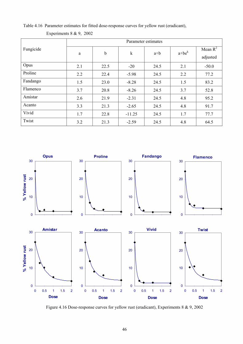
46
Table 4.16 Parameter estimates for fitted dose-response curves for yellow rust (eradicant),
Experiments 8 & 9, 2002
Parameter estimates
Fungicide a b k a+b a+bek
Mean R2
adjusted
Opus 2.1 22.5 -20 24.5 2.1 -50.0 Proline 2.2 22.4 -5.98 24.5 2.2 77.2 Fandango 1.5 23.0 -8.28 24.5 1.5 83.2 Flamenco 3.7 20.8 -8.26 24.5 3.7 52.8 Amistar 2.6 21.9 -2.31 24.5 4.8 95.2 Acanto 3.3 21.3 -2.65 24.5 4.8 91.7 Vivid 1.7 22.8 -11.25 24.5 1.7 77.7 Twist 3.2 21.3 -2.59 24.5 4.8 64.5
Figure 4.16 Dose-response curves for yellow rust (eradicant), Experiments 8 & 9, 2002
Opus
0
10
20
30
% Y
ello
w ru
st
Amistar
0
10
20
30
0 0.5 1 1.5 2
Dose
% Y
ello
w ru
st
Proline
0
10
20
30Fandango
0
10
20
30
Acanto
0
10
20
30
0 0.5 1 1.5 2
Dose
Vivid
0
10
20
30
0 0.5 1 1.5 2
Dose
Flamenco
0
10
20
30
Twist
0
10
20
30
0 0.5 1 1.5 2
Dose
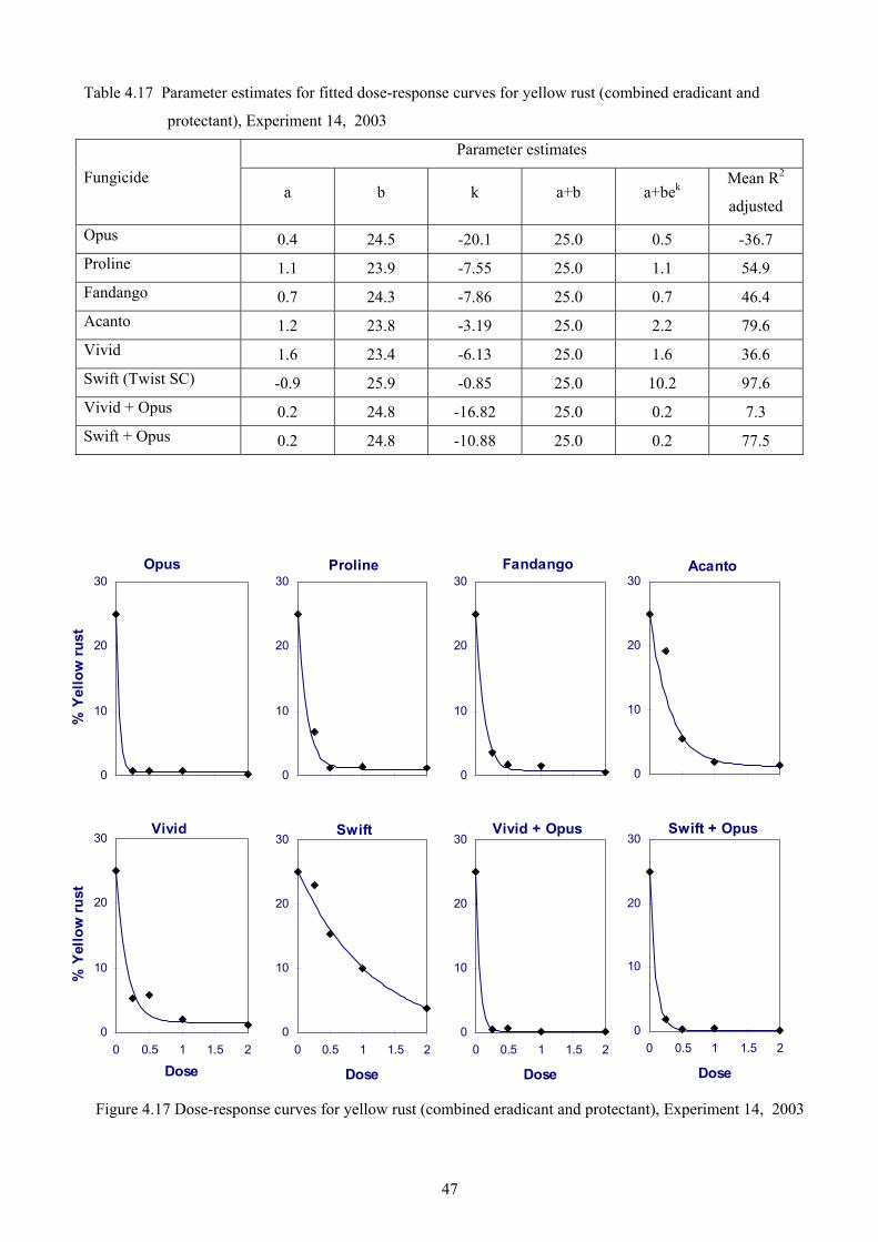
47
Table 4.17 Parameter estimates for fitted dose-response curves for yellow rust (combined eradicant and
protectant), Experiment 14, 2003
Parameter estimates
Fungicide a b k a+b a+bek
Mean R2
adjusted
Opus 0.4 24.5 -20.1 25.0 0.5 -36.7 Proline 1.1 23.9 -7.55 25.0 1.1 54.9 Fandango 0.7 24.3 -7.86 25.0 0.7 46.4 Acanto 1.2 23.8 -3.19 25.0 2.2 79.6 Vivid 1.6 23.4 -6.13 25.0 1.6 36.6 Swift (Twist SC) -0.9 25.9 -0.85 25.0 10.2 97.6 Vivid + Opus 0.2 24.8 -16.82 25.0 0.2 7.3 Swift + Opus 0.2 24.8 -10.88 25.0 0.2 77.5
Figure 4.17 Dose-response curves for yellow rust (combined eradicant and protectant), Experiment 14, 2003
Opus
0
10
20
30
% Y
ello
w ru
st
Vivid
0
10
20
30
0 0.5 1 1.5 2
Dose
% Y
ello
w ru
st
Proline
0
10
20
30Fandango
0
10
20
30
Swift
0
10
20
30
0 0.5 1 1.5 2
Dose
Vivid + Opus
0
10
20
30
0 0.5 1 1.5 2
Dose
Acanto
0
10
20
30
Swift + Opus
0
10
20
30
0 0.5 1 1.5 2
Dose

48
Table 4.18 Parameter estimates for fitted dose response curves for yellow rust (combined eradicant and
protectant), Experiment 21, 2004
Parameter estimates
Fungicide a b k a+b a+bek
Mean R2
adjusted
Opus 0.2 19.8 -16.0 19.9 0.2 90.5 Proline 0.1 19.8 -16.0 19.9 0.1 77.5 Fandango 0.2 19.7 -16.0 19.9 0.2 98.9 Tracker 0.2 19.7 -13.8 19.9 0.2 99.6 Amistar 0.5 19.4 -8.4 19.9 0.5 81.9 Vivid 0.7 19.2 -13.4 19.9 0.7 96.6 Swift (Twist SC) 2.4 17.5 -14.1 19.9 2.4 63.6 Charisma 1.4 18.5 -5.1 19.9 1.5 95.6
Figure 4.18 Dose-response curves for yellow rust (combined eradicant and protectant), Experiment 21, 2004
Opus
0
5
10
15
20
% Y
ello
w ru
st
Amistar
0
5
10
15
20
0 0.5 1 1.5 2
Dose
% Y
ello
w ru
st
Proline
0
5
10
15
20Fandango
0
5
10
15
20
Vivid
0
5
10
15
20
0 0.5 1 1.5 2
Dose
Swift
0
5
10
15
20
0 0.5 1 1.5 2
Dose
Tracker
0
5
10
15
20
Charisma
0
5
10
15
20
0 0.5 1 1.5 2
Dose
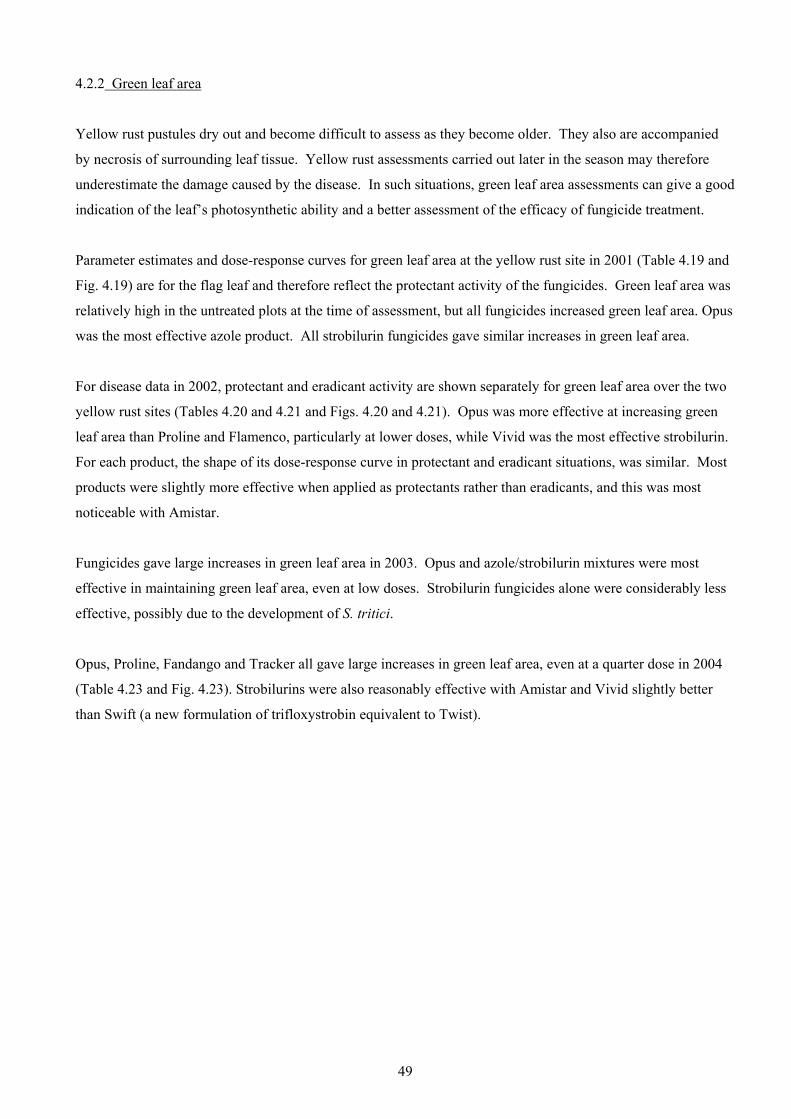
49
4.2.2 Green leaf area
Yellow rust pustules dry out and become difficult to assess as they become older. They also are accompanied
by necrosis of surrounding leaf tissue. Yellow rust assessments carried out later in the season may therefore
underestimate the damage caused by the disease. In such situations, green leaf area assessments can give a good
indication of the leaf’s photosynthetic ability and a better assessment of the efficacy of fungicide treatment.
Parameter estimates and dose-response curves for green leaf area at the yellow rust site in 2001 (Table 4.19 and
Fig. 4.19) are for the flag leaf and therefore reflect the protectant activity of the fungicides. Green leaf area was
relatively high in the untreated plots at the time of assessment, but all fungicides increased green leaf area. Opus
was the most effective azole product. All strobilurin fungicides gave similar increases in green leaf area.
For disease data in 2002, protectant and eradicant activity are shown separately for green leaf area over the two
yellow rust sites (Tables 4.20 and 4.21 and Figs. 4.20 and 4.21). Opus was more effective at increasing green
leaf area than Proline and Flamenco, particularly at lower doses, while Vivid was the most effective strobilurin.
For each product, the shape of its dose-response curve in protectant and eradicant situations, was similar. Most
products were slightly more effective when applied as protectants rather than eradicants, and this was most
noticeable with Amistar.
Fungicides gave large increases in green leaf area in 2003. Opus and azole/strobilurin mixtures were most
effective in maintaining green leaf area, even at low doses. Strobilurin fungicides alone were considerably less
effective, possibly due to the development of S. tritici.
Opus, Proline, Fandango and Tracker all gave large increases in green leaf area, even at a quarter dose in 2004
(Table 4.23 and Fig. 4.23). Strobilurins were also reasonably effective with Amistar and Vivid slightly better
than Swift (a new formulation of trifloxystrobin equivalent to Twist).

50
Table 4.19 Parameter estimates for fitted dose response curves for green leaf area, Experiment 2, 2001
Parameter estimates
Fungicide a b k a+b a+bek
Mean R2
adjusted
Opus 98.7 -10.1 -10.9 88.6 98.7 99.4 Caramba 96.7 -8.1 -20 88.6 96.8 82.4 Amistar 98.0 -9.4 -7.9 88.6 98.0 97.2 Vivid 96.9 -8.3 -7.65 88.6 97.0 95.9 Proline 97.6 -9.0 -20 88.6 97.6 98.9 Flamenco 96.3 -7.7 -20 88.6 96.3 82.0 Acanto 98.0 -9.4 -20 88.6 98.0 99.4 Twist 97.9 -9.3 -8.1 88.6 98.0 92.4
Figure 4.19 Dose-response curves for green leaf area, Experiment 2, 2001
Opus
85
90
95
100
% G
reen
leaf
are
a
Proline
85
90
95
100
0 0.5 1 1.5 2
Dose
% G
reen
leaf
are
a
Caramba
85
90
95
100Amistar
85
90
95
100
Flamenco
85
90
95
100
0 0.5 1 1.5 2
Dose
Acanto
85
90
95
100
0 0.5 1 1.5 2
Dose
Vivid
85
90
95
100
Twist
85
90
95
100
0 0.5 1 1.5 2
Dose
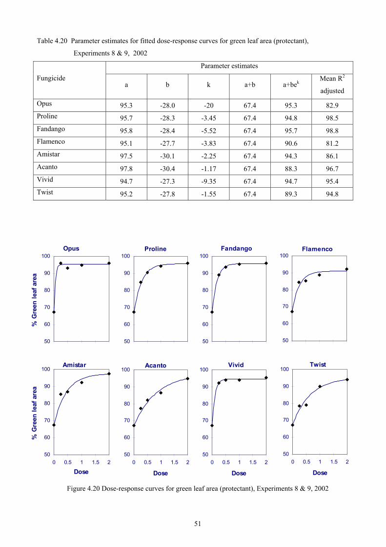
51
Table 4.20 Parameter estimates for fitted dose-response curves for green leaf area (protectant),
Experiments 8 & 9, 2002
Parameter estimates
Fungicide a b k a+b a+bek
Mean R2
adjusted
Opus 95.3 -28.0 -20 67.4 95.3 82.9 Proline 95.7 -28.3 -3.45 67.4 94.8 98.5 Fandango 95.8 -28.4 -5.52 67.4 95.7 98.8 Flamenco 95.1 -27.7 -3.83 67.4 90.6 81.2 Amistar 97.5 -30.1 -2.25 67.4 94.3 86.1 Acanto 97.8 -30.4 -1.17 67.4 88.3 96.7 Vivid 94.7 -27.3 -9.35 67.4 94.7 95.4 Twist 95.2 -27.8 -1.55 67.4 89.3 94.8
Figure 4.20 Dose-response curves for green leaf area (protectant), Experiments 8 & 9, 2002
Opus
50
60
70
80
90
100
% G
reen
leaf
are
a
Amistar
50
60
70
80
90
100
0 0.5 1 1.5 2
Dose
% G
reen
leaf
are
a
Proline
50
60
70
80
90
100Fandango
50
60
70
80
90
100
Acanto
50
60
70
80
90
100
0 0.5 1 1.5 2
Dose
Vivid
50
60
70
80
90
100
0 0.5 1 1.5 2
Dose
Flamenco
50
60
70
80
90
100
Twist
50
60
70
80
90
100
0 0.5 1 1.5 2
Dose

52
Table 4.21 Parameter estimates for fitted dose-response curves for green leaf area (eradicant),
Experiments 8 & 9, 2002
Parameter estimates
Fungicide a b k a+b a+bek
Mean R2
adjusted
Opus 93.1 -39.6 -20 53.5 93.1 98.6 Proline 93.1 -39.6 -4.92 53.5 83.4 95.3 Fandango 93.3 -39.7 -8.13 53.5 61.2 95.2 Flamenco 89.6 -36.1 -7.78 53.5 65.2 96.7 Amistar 91.5 -38.0 -2.91 53.5 87.7 94.8 Acanto 90.7 -37.1 -3.19 53.5 86.3 94.6 Vivid 93.7 -40.2 -12.73 53.5 75.7 99.4 Twist 91.9 -38.4 -3.5 53.5 53.9 81.1
Figure 4.21 Dose-response curves for green leaf area (eradicant), Experiments 8 & 9, 2002
Opus
50
60
70
80
90
100
% G
reen
leaf
are
a
Amistar
50
60
70
80
90
100
0 0.5 1 1.5 2
Dose
% G
reen
leaf
are
a
Proline
50
60
70
80
90
100Fandango
50
60
70
80
90
100
Acanto
50
60
70
80
90
100
0 0.5 1 1.5 2
Dose
Vivid
50
60
70
80
90
100
0 0.5 1 1.5 2
Dose
Flamenco
50
60
70
80
90
100
Twist
50
60
70
80
90
100
0 0.5 1 1.5 2
Dose

53
Table 4.22 Parameter estimates for fitted dose-response curves for green leaf area (combined eradicant and
protectant), Experiment 14, 2003
Parameter estimates
Fungicide a b k a+b a+bek
Mean R2
adjusted
Opus 95.7 -48.9 -12.44 46.8 95.7 91.1 Proline 94.1 -47.3 -3.95 46.8 93.1 99.9 Fandango 93.2 -46.5 -12.79 46.8 93.2 73.1 Acanto 91.1 -44.3 -2.39 46.8 87.0 71.3 Vivid 86.0 -39.2 -4.89 46.8 85.7 82.2 Swift (Twist SC) 35.8 11.0 0.75 46.8 59.0 94.1 Vivid + Opus 96.1 -49.3 -13.15 46.8 96.1 95.7 Swift + Opus 96.7 -50.0 -7.28 46.8 96.7 92.5
Table 4.22 Dose-response curves for green leaf area (combined eradicant and protectant), Experiment 14, 2003
Opus
40
50
60
70
80
90
100
% G
reen
leaf
are
a
Vivid
40
50
60
70
80
90
100
0 0.5 1 1.5 2
Dose
% G
reen
leaf
are
a
Proline
40
50
60
70
80
90
100Fandango
40
50
60
70
80
90
100
Swift
40
50
60
70
80
90
100
0 0.5 1 1.5 2
Dose
Vivid + Opus
40
50
60
70
80
90
100
0 0.5 1 1.5 2
Dose
Acanto
40
50
60
70
80
90
100
Swift + Opus
40
50
60
70
80
90
100
0 0.5 1 1.5 2
Dose

54
Table 4.23 Parameter estimates for fitted dose-response curves for green leaf area (combined eradicant and
protectant), Experiment 21, 2004
Parameter estimates
Fungicide a b k a+b a+bek
Mean R2
adjusted
Opus 98.2 -32.1 -13.0 66.1 98.2 88.4 Proline 99.1 -32.9 -16.0 66.1 99.1 93.9 Fandango 98.8 -32.7 -15.3 66.1 98.8 100.0 Tracker 98.4 -32.3 -10.8 66.1 98.4 99.8 Amistar 95.7 -29.6 -6.4 66.1 95.6 94.8 Vivid 95.2 -29.0 -9.4 66.1 95.2 98.9 Swift (Twist SC) 90.8 -24.7 -16.0 66.1 90.8 85.8 Charisma 95.3 -29.2 -3.9 66.1 94.7 98.5
Figure 4.23 Dose-response curves for green leaf area (combined eradicant and protectant), Experiment 21,
2004
Opus
60
70
80
90
100
% G
reen
leaf
are
a
Amistar
60
70
80
90
100
0 0.5 1 1.5 2
Dose
% G
reen
leaf
are
a
Proline
60
70
80
90
100Fandango
60
70
80
90
100
Vivid
60
70
80
90
100
0 0.5 1 1.5 2
Dose
Swift
60
70
80
90
100
0 0.5 1 1.5 2
Dose
Tracker
60
70
80
90
100
Charisma
60
70
80
90
100
0 0.5 1 1.5 2
Dose

55
4.2.3 Grain yield
The yield data at Terrington in 2001 (Table 4.24 and Fig. 4.24) are difficult to reconcile with the yellow rust
activity of treatments. Most products increased yield by about 1.0 t/ha at quarter or half dose, and beyond that
point, the fitted dose-response curve was flat. Exceptions were Caramba and Twist, which, although not giving
the best yellow rust control, continued to increase yield at higher doses.
Mean yield data over two sites (Terrington and Morley) are presented in Table 4.25 and Fig. 4.25. At each
dose, Opus gave a greater yield increase than any other product. The benefit from the addition of fluoxastrobin
to prothioconazole in Fandango, compared with Proline, which was evident in the rust assessments, was also
reflected in improved yield.
The performance of Proline relative to Opus improved in 2003, although it was still less effective at quarter dose
(Table 4.26 and Fig. 4.26). The new formulation of trifloxystrobin (Swift), used for the first time in 2003,
appeared to be less effective than the original formulation (Twist). However, mixtures of both Swift plus Opus
and Vivid plus Opus gave good yield increases.
In 2004, the experiment at Terrington (Experiment 21) was severely affected by S. tritici in addition to yellow
rust and the yield data therefore reflect the level of control of both diseases. The relatively poor performance of
Amistar, Swift and Vivid may be explained by poor control of strobilurin-resistant S. tritici (Table 4.27 and Fig.
4.27). Proline, Tracker and Fandango gave yield responses similar to Opus. Proline gave poorer control of
yellow rust than Opus but had similar yield.
Mean yield data across all yellow rust sites between 2001 and 2003 are presented in Table 4.28 and Fig. 4.28.
Data for 2004 have not been included because of the overriding effect of S. tritici in that year. Of the azole
fungicides, Opus gave the overall greatest yield increases. All strobilurin products, with the exception of Vivid,
gave yield increases up to double dose; the dose response curve for Vivid flattened out at half dose. The new
formulation of trifloxystrobin did not appear to offer any yield advantage over the original formulation. The
greatest mean yield increases over the yellow rust sites were given by the azole/strobilurin mixtures, Vivid +
Opus, Swift + Opus and Fandango.
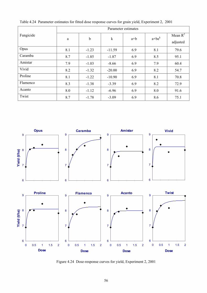
56
Table 4.24 Parameter estimates for fitted dose response curves for grain yield, Experiment 2, 2001
Parameter estimates
Fungicide a b k a+b a+bek
Mean R2
adjusted
Opus 8.1 -1.23 -11.59 6.9 8.1 79.6 Caramba 8.7 -1.85 -1.87 6.9 8.5 95.1 Amistar 7.9 -1.03 -8.66 6.9 7.9 60.4 Vivid 8.2 -1.32 -20.00 6.9 8.2 54.7 Proline 8.1 -1.22 -10.90 6.9 8.1 70.8 Flamenco 8.3 -1.38 -3.39 6.9 8.2 72.9 Acanto 8.0 -1.12 -6.96 6.9 8.0 91.6 Twist 8.7 -1.78 -3.09 6.9 8.6 75.1
Figure 4.24 Dose-response curves for yield, Experiment 2, 2001
Opus
6
7
8
9
Yie
ld (t
/ha)
Proline
6
7
8
9
0 0.5 1 1.5 2
Dose
Yiel
d (t/
ha)
Caramba
6
7
8
9Amistar
6
7
8
9
Flamenco
6
7
8
9
0 0.5 1 1.5 2
Dose
Acanto
6
7
8
9
0 0.5 1 1.5 2
Dose
Vivid
6
7
8
9
Twist
6
7
8
9
0 0.5 1 1.5 2
Dose
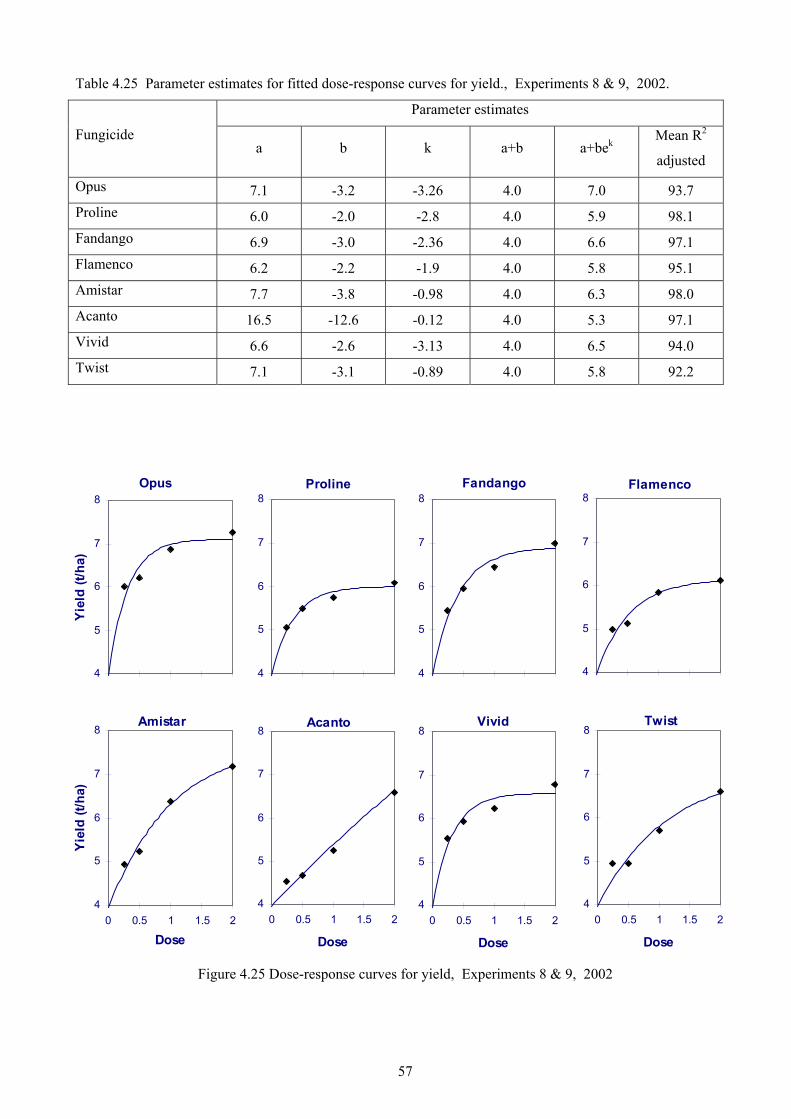
57
Table 4.25 Parameter estimates for fitted dose-response curves for yield., Experiments 8 & 9, 2002.
Parameter estimates
Fungicide a b k a+b a+bek
Mean R2
adjusted
Opus 7.1 -3.2 -3.26 4.0 7.0 93.7 Proline 6.0 -2.0 -2.8 4.0 5.9 98.1 Fandango 6.9 -3.0 -2.36 4.0 6.6 97.1 Flamenco 6.2 -2.2 -1.9 4.0 5.8 95.1 Amistar 7.7 -3.8 -0.98 4.0 6.3 98.0 Acanto 16.5 -12.6 -0.12 4.0 5.3 97.1 Vivid 6.6 -2.6 -3.13 4.0 6.5 94.0 Twist 7.1 -3.1 -0.89 4.0 5.8 92.2
Figure 4.25 Dose-response curves for yield, Experiments 8 & 9, 2002
Opus
4
5
6
7
8
Yie
ld (t
/ha)
Amistar
4
5
6
7
8
0 0.5 1 1.5 2
Dose
Yiel
d (t/
ha)
Proline
4
5
6
7
8Fandango
4
5
6
7
8
Acanto
4
5
6
7
8
0 0.5 1 1.5 2
Dose
Vivid
4
5
6
7
8
0 0.5 1 1.5 2
Dose
Flamenco
4
5
6
7
8
Twist
4
5
6
7
8
0 0.5 1 1.5 2
Dose

58
Table 4.26 Parameter estimates for fitted dose-response curves for yield, Experiment 14, 2003
Parameter estimates
Fungicide a b k a+b a+bek
Mean R2
adjusted
Opus 8.9 -2.5 -13.14 6.4 8.9 88.9 Proline 8.8 -2.4 -4.51 6.4 8.8 98.9 Fandango 9.1 -2.7 -6.43 6.4 9.1 93.2 Acanto 8.6 -2.2 -2.66 6.4 8.4 92.4 Vivid 8.4 -2.0 -4.24 6.4 8.4 94.9 Swift (Twist SC) 8.1 -1.7 -1.51 6.4 7.7 90.2 Vivid + Opus 9.4 -3.0 -9.16 6.4 9.4 98.1 Swift + Opus 9.3 -2.9 -5.41 6.4 9.3 99.4
Figure 4.26 Dose-response curves for yield, Experiment 14, 2003
Opus
6
7
8
9
10
Yie
ld (t
/ha)
Vivid
6
7
8
9
10
0 0.5 1 1.5 2
Dose
Yiel
d (t/
ha)
Proline
6
7
8
9
10Fandango
6
7
8
9
10
Swift (Twist SC)
6
7
8
9
10
0 0.5 1 1.5 2
Dose
Vivid + Opus
6
7
8
9
10
0 0.5 1 1.5 2
Dose
Acanto
6
7
8
9
10
Swift + Opus
6
7
8
9
10
0 0.5 1 1.5 2
Dose

59
Table 4.27 Parameter estimates for fitted dose-response curves for yield, Experiment 21, 2004
Parameter estimates
Fungicide a b k a+b a+bek
Mean R2
adjusted
Opus 9.0 -4.0 -5.0 5.0 9.0 93.5
Proline 8.7 -3.7 -6.5 5.0 8.7 99.2
Fandango 9.2 -4.2 -5.3 5.0 9.2 97.8
Tracker 9.2 -4.2 -4.1 5.0 9.2 99.7
Amistar 7.3 -2.3 -3.9 5.0 7.3 97.4
Vivid 7.2 -2.2 -4.3 5.0 7.2 97.3
Swift 6.5 -1.4 -10.6 5.0 6.5 93.5
Charisma 7.4 -2.3 -2.0 5.0 7.1 100.0
Figure 4.27 Dose-response curves for yield, Experiment 21, 2004
Opus
5
6
7
8
9
10
Yiel
d t/h
a
Amistar
5
6
7
8
9
10
0 0.5 1 1.5 2
Dose
Yie
ld t/
ha
Proline
5
6
7
8
9
10Fandango
5
6
7
8
9
10
Vivid
5
6
7
8
9
10
0 0.5 1 1.5 2
Dose
Swift
5
6
7
8
9
10
0 0.5 1 1.5 2
Dose
Tracker
5
6
7
8
9
10
Charisma
5
6
7
8
9
10
0 0.5 1 1.5 2
Dose

60
Table 4.28 Parameter estimates for fitted dose-response curves for yield, mean data for all yellow rust sites
2001-2003 (Experiment s 2, 8, 9 & 14)
Parameter estimates
Fungicide a b k a+b a+bek
Mean R2
adjusted
Opus 7.75 -2.45 -5.02 5.3 7.73 96.2 Caramba 7.53 -2.23 -2.87 5.3 7.40 95.9 Flamenco 7.26 -1.96 -2.42 5.3 7.09 95.1 Proline 7.20 -1.90 -4.01 5.3 7.16 99.5 Fandango 7.95 -2.65 -3.03 5.3 7.83 96.8 Acanto 7.50 -2.20 -1.30 5.3 6.90 97.9 Amistar 7.99 -2.69 -1.46 5.3 7.37 96.3 Vivid 7.30 -2.00 -5.74 5.3 7.30 95.7 Twist 7.90 -2.60 -1.34 5.3 7.22 92.1 Swift (Twist SC) 6.91 -1.61 -1.05 5.3 6.35 89.0 Vivid + Opus 8.05 -2.75 -8.71 5.3 8.05 98.5 Swift + Opus 7.92 -2.62 -5.07 5.3 7.91 99.5
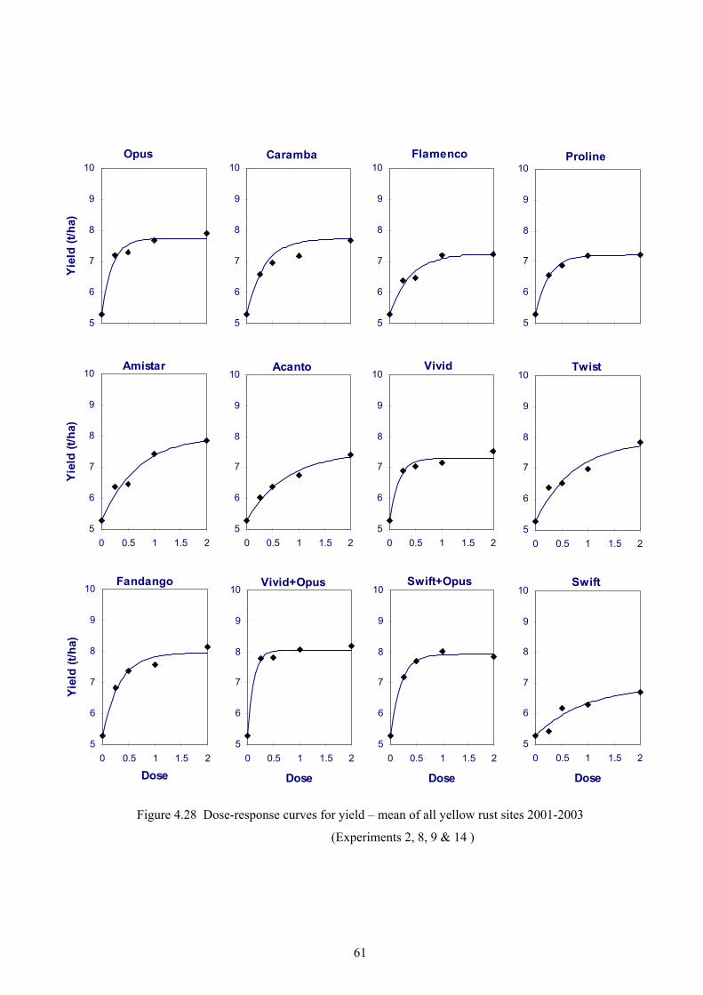
61
Figure 4.28 Dose-response curves for yield – mean of all yellow rust sites 2001-2003
(Experiments 2, 8, 9 & 14 )
Opus
5
6
7
8
9
10
Yiel
d (t/
ha)
Amistar
5
6
7
8
9
10
0 0.5 1 1.5 2
Yiel
d (t/
ha)
Caramba
5
6
7
8
9
10Flamenco
5
6
7
8
9
10
Acanto
5
6
7
8
9
10
0 0.5 1 1.5 2
Vivid
5
6
7
8
9
10
0 0.5 1 1.5 2
Fandango
5
6
7
8
9
10
0 0.5 1 1.5 2
Dose
Yiel
d (t/
ha)
Vivid+Opus
5
6
7
8
9
10
0 0.5 1 1.5 2
Dose
Swift+Opus
5
6
7
8
9
10
0 0.5 1 1.5 2
Dose
Swift
5
6
7
8
9
10
0 0.5 1 1.5 2
Dose
Proline
5
6
7
8
9
10
Twist
5
6
7
8
9
10
0 0.5 1 1.5 2

62
4.2.4 Specific weights
Some of the specific weight data for Terrington in 2001 were variable and in particular, the fitted curves for
Caramba and Flamenco were not good fits with the observed data (Table 4.29 and Fig. 4.29). Specific weight
curves for other products were generally better fits and are similar in shape to the yield curves. Most products
did not increase specific weight beyond full dose, but Twist was an exception giving an additional 1.0 kg/hl at
double dose.
In 2002, the specific weight dose-response curves fitted the observed mean data for Terrington and Morley well
(Table 4.30 and Fig. 4.30). Specific weight was not increased above full dose for azole products, but
strobilurins gave increases in specific weight up to double dose, much in line with the yield data.
The shapes of the fitted dose-response curves for specific weights at Terrington in 2003 (Table 4.31 and Fig.
4.31) correlated well with the yield curves. The poorer performance of Proline compared with Opus at quarter
doses was also evident. Swift was slightly less effective in increasing specific weight than other strobilurin
fungicides at the 2003 site.
In 2004, however, Swift gave considerably greater specific weights than other strobilurins, corresponding to its
yield advantage at this site where S. tritici was also a factor. (Table 4.32 and Fig. 4.32). Opus was again
superior to Proline (and Fandango). Tracker and Charisma gave the greatest increases in specific weights
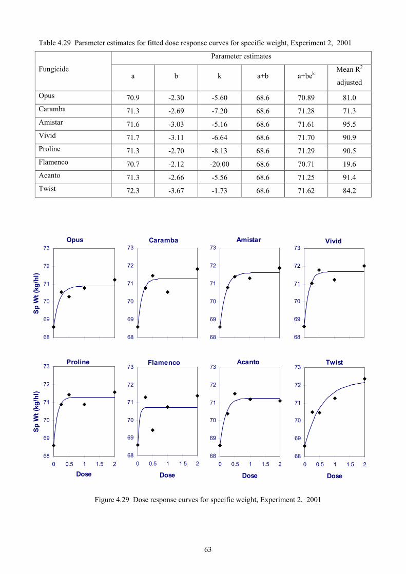
63
Table 4.29 Parameter estimates for fitted dose response curves for specific weight, Experiment 2, 2001
Parameter estimates
Fungicide a b k a+b a+bek
Mean R2
adjusted
Opus 70.9 -2.30 -5.60 68.6 70.89 81.0 Caramba 71.3 -2.69 -7.20 68.6 71.28 71.3 Amistar 71.6 -3.03 -5.16 68.6 71.61 95.5 Vivid 71.7 -3.11 -6.64 68.6 71.70 90.9 Proline 71.3 -2.70 -8.13 68.6 71.29 90.5 Flamenco 70.7 -2.12 -20.00 68.6 70.71 19.6 Acanto 71.3 -2.66 -5.56 68.6 71.25 91.4 Twist 72.3 -3.67 -1.73 68.6 71.62 84.2
Figure 4.29 Dose response curves for specific weight, Experiment 2, 2001
Opus
68
69
70
71
72
73
Sp W
t (kg
/hl)
Proline
68
69
70
71
72
73
0 0.5 1 1.5 2
Dose
Sp
Wt (
kg/h
l)
Caramba
68
69
70
71
72
73Amistar
68
69
70
71
72
73
Flamenco
68
69
70
71
72
73
0 0.5 1 1.5 2
Dose
Acanto
68
69
70
71
72
73
0 0.5 1 1.5 2
Dose
Vivid
68
69
70
71
72
73
Twist
68
69
70
71
72
73
0 0.5 1 1.5 2
Dose

64
Table 4.30 Parameter estimates for fitted dose-response curves for specific weight, Experiments 8 & 9, 2002.
Parameter estimates
Fungicide a b k a+b a+bek
Mean R2
adjusted
Opus 66.1 -5.4 -2.68 60.7 65.7 99.5 Proline 64.7 -4.0 -3.74 60.7 64.6 95.5 Fandango 66.2 -5.5 -2.45 60.7 65.7 91.5 Flamenco 64.0 -3.3 -4.6 60.7 63.9 82.1 Amistar 69.6 -8.9 -0.66 60.7 65.0 98.2 Acanto 69.0 -8.4 -0.41 60.7 63.5 98.4 Vivid 65.6 -4.9 -1.72 60.7 64.7 98.9 Twist 69.7 -9.0 -0.46 60.7 64.0 99.3
Figure 4.30 Dose-response curves for specific weight, Experiments 8 & 9, 2002
Opus
60
61
62
63
64
65
66
67
68
Sp W
t (kg
/hl)
Amistar
60
61
62
63
64
65
66
67
68
0 0.5 1 1.5 2
Dose
Sp
Wt (
kg/h
l)
Proline
60
61
62
63
64
65
66
67
68Fandango
60
61
62
63
64
65
66
67
68
Acanto
60
61
62
63
64
65
66
67
68
0 0.5 1 1.5 2
Dose
Vivid
60
61
62
63
64
65
66
67
68
0 0.5 1 1.5 2
Dose
Flamenco
60
61
62
63
64
65
66
67
68
Twist
60
61
62
63
64
65
66
67
68
0 0.5 1 1.5 2
Dose

65
Table 4.31 Parameter estimates for fitted dose-response curves for specific weight, Experiment 14, 2003
Parameter estimates
Fungicide a b k a+b a+bek
Mean R2
adjusted
Opus 66.6 -5.38 -9.96 61.2 66.6 96.9 Proline 66.1 -4.87 -3.4 61.2 65.9 77.9 Fandango 65.6 -4.43 -19.88 61.2 65.6 61.9 Acanto 65.1 -3.89 -2.73 61.2 64.8 67.8 Vivid 65.6 -4.42 -2.83 61.2 65.5 62.1 Swift (Twist SC) 65.0 -3.76 -2.24 61.2 64.6 95.4 Vivid + Opus 67.0 -5.77 -20 61.2 67.0 98.4 Swift + Opus 66.9 -5.66 -5.26 61.2 66.8 96.1
Figure 4.31 Dose-response curves for specific weight, Experiment 14, 2003
Opus
60
61
62
63
64
65
66
67
68
Sp W
t (kg
/hl)
Vivid
60
61
62
63
64
65
66
67
68
0 0.5 1 1.5 2
Dose
Sp
Wt (
kg/h
l)
Proline
60
61
62
63
64
65
66
67
68Fandango
60
61
62
63
64
65
66
67
68
Swift (Twist SC)
60
61
62
63
64
65
66
67
68
0 0.5 1 1.5 2
Dose
Vivid + Opus
60
61
62
63
64
65
66
67
68
0 0.5 1 1.5 2
Dose
Acanto
60
61
62
63
64
65
66
67
68
Swift + Opus
60
61
62
63
64
65
66
67
68
0 0.5 1 1.5 2
Dose

66
Table 4.32 Parameter estimates for fitted dose-response curves for specific weight, Experiment 21, 2004
Parameter estimates
Fungicide a b k a+b a+bek
Mean R2
adjusted
Opus 74.1 -8.0 -9.7 66.1 74.1 94.5 Proline 71.8 -5.7 -3.2 66.1 71.6 65.4 Fandango 69.8 -3.7 -1.8 66.1 69.2 54.0 Tracker 75.7 -9.6 -3.4 66.1 75.4 97.0 Amistar 70.2 -4.1 -16.0 66.1 70.2 72.8 Vivid 68.5 -2.4 -6.2 66.1 68.5 78.6 Swift (Twist SC) 73.5 -7.3 -6.2 66.1 73.4 98.4 Charisma 75.0 -8.9 -7.1 66.1 75.0 99.5
Figure 4.32 Dose-response curves for specific weight, Experiment 21, 2004
Opus
666768697071727374757677
Sp W
t (kg
/hl)
Amistar
666768697071727374757677
0 0.5 1 1.5 2
Dose
Sp
Wt (
kg/h
l)
Proline
666768697071727374757677
Fandango
666768697071727374757677
Vivid
666768697071727374757677
0 0.5 1 1.5 2
Dose
Swift (Twist SC)
666768697071727374757677
0 0.5 1 1.5 2
Dose
Tracker
666768697071727374757677
Charisma
666768697071727374757677
0 0.5 1 1.5 2
Dose

67
4.3 Septoria tritici experiments
4.3.1 Disease control
There were a larger number of sites targeting S. tritici than any other disease, and it is therefore possible to
present cross-site mean data for some years. By assessing each leaf layer separately, it is also possible to show
data for the protectant and eradicant activity of fungicides.
The cross-site analysis for 2001 (Suffolk, Norfolk and Fife) showed that Opus was equally effective as a
protectant or eradicant treatment (Tables 4.33 and 4.34 and Figures 4.33 and 4.34). Proline and Flamenco were
more effective as protectants, while Caramba gave better control of S. tritici when applied as an eradicant, at
least at higher doses. Most of the strobilurin fungicides (Amistar, Acanto and Twist) were more effective when
applied as protectants. Vivid was equally effective applied as a protectant or eradicant.
There was only one S. tritici site in 2002 (Fife). All fungicides applied as protectant sprays gave good control of
relatively low levels of disease. Proline, Twist and Vivid gave almost complete control at a quarter dose (Table
4.35 and Figure 4.35). Levels of S. tritici were greater on lower leaves but most fungicides applied as eradicant
sprays continued to give good control at half or full dose. Amistar was the weakest product (Table 4.36 and
Figure 4.36).
The first indication of poor control of S. tritici by strobilurin fungicides was seen in 2003. Mean data from three
sites in eastern England, Scotland and Ireland, showed that Acanto, Swift and Vivid were less effective
protectant sprays than in previous years (Table 4.37 and Figure 4.37). When applied as eradicant sprays, these
strobilurins gave very poor control of S. tritici (Table 4.38 and Figure 4.38). Mixture of strobilurins with azoles
(Fandango, Swift + Opus and Vivid + Opus) gave better disease control.
By 2004, Vivid and Swift were giving very little control of S. tritici at a quarter dose, and increasing dose, even
to double the label dose had no effect (Tables 4.39 and 4.40 and Figures 4.39 and 4.40). The lack of dose
response beyond a quarter dose by the strobilurins was also seen when Swift and Vivid were applied in mixtures
with half dose Opus. The level of control from the mixture was just slightly better than the equivalent control
given by half dose Opus alone. There was also an indication that azoles such as Opus, were becoming less
effective against S. tritici.

68
Table 4.33 Parameter estimates for fitted dose response curves for S. tritici (protectant)
Experiments 3, 4 & 5, 2001
Parameter estimates
Fungicide a b k a+b a+bek
Mean R2
adjusted
Opus 5.9 20.3 -3.53 26.2 6.5 95.2 Proline 4.4 21.8 -2.05 26.2 7.2 98.6 Caramba 11.0 15.3 -7.2 26.2 11.0 89.7 Flamenco 8.5 17.7 -2.96 26.2 9.5 86.0 Amistar 7.7 18.5 -3.42 26.2 8.3 99.5 Acanto 5.3 20.9 -4.06 26.2 5.7 80.0 Vivid 7.4 18.9 -6.49 26.2 7.4 96.9 Twist 4.2 22.0 -11.29 26.2 4.2 99.7
Figure 4.33 Dose-response curves for S. tritici (protectant), Experiments 3, 4 & 5, 2001
Opus
0
5
10
15
20
25
30
% S
. tri
tici
Amistar
0
5
10
15
20
25
30
0 0.5 1 1.5 2
Dose
% S
. tri
tici
Proline
0
5
10
15
20
25
30Caramba
0
5
10
15
20
25
30
Acanto
0
5
10
15
20
25
30
0 0.5 1 1.5 2
Dose
Vivid
0
5
10
15
20
25
30
0 0.5 1 1.5 2
Dose
Flamenco
0
5
10
15
20
25
30
Twist
0
5
10
15
20
25
30
0 0.5 1 1.5 2
Dose
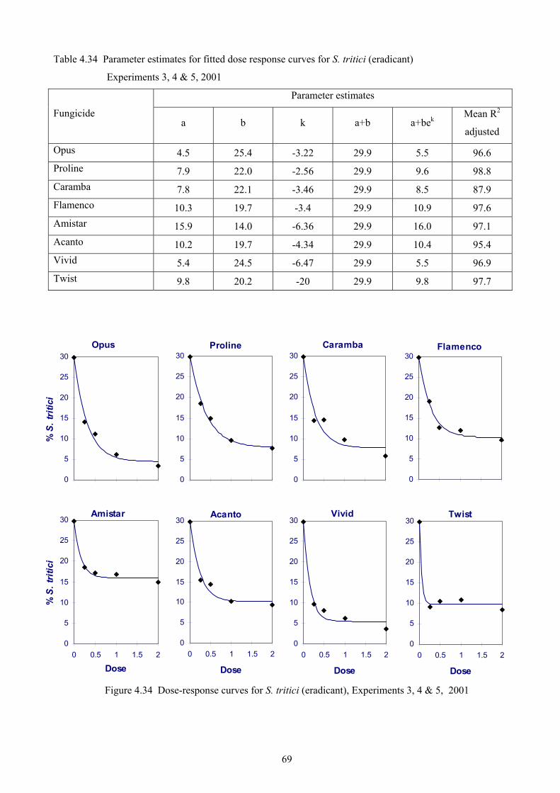
69
Table 4.34 Parameter estimates for fitted dose response curves for S. tritici (eradicant)
Experiments 3, 4 & 5, 2001
Parameter estimates
Fungicide a b k a+b a+bek
Mean R2
adjusted
Opus 4.5 25.4 -3.22 29.9 5.5 96.6 Proline 7.9 22.0 -2.56 29.9 9.6 98.8 Caramba 7.8 22.1 -3.46 29.9 8.5 87.9 Flamenco 10.3 19.7 -3.4 29.9 10.9 97.6 Amistar 15.9 14.0 -6.36 29.9 16.0 97.1 Acanto 10.2 19.7 -4.34 29.9 10.4 95.4 Vivid 5.4 24.5 -6.47 29.9 5.5 96.9 Twist 9.8 20.2 -20 29.9 9.8 97.7
Figure 4.34 Dose-response curves for S. tritici (eradicant), Experiments 3, 4 & 5, 2001
Opus
0
5
10
15
20
25
30
% S
. tri
tici
Amistar
0
5
10
15
20
25
30
0 0.5 1 1.5 2
Dose
% S
. tri
tici
Proline
0
5
10
15
20
25
30Caramba
0
5
10
15
20
25
30
Acanto
0
5
10
15
20
25
30
0 0.5 1 1.5 2
Dose
Vivid
0
5
10
15
20
25
30
0 0.5 1 1.5 2
Dose
Flamenco
0
5
10
15
20
25
30
Twist
0
5
10
15
20
25
30
0 0.5 1 1.5 2
Dose
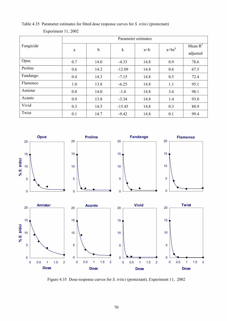
70
Table 4.35 Parameter estimates for fitted dose response curves for S. tritici (protectant)
Experiment 11, 2002
Parameter estimates
Fungicide a b k a+b a+bek
Mean R2
adjusted
Opus 0.7 14.0 -4.33 14.8 0.9 78.6 Proline 0.6 14.2 -12.09 14.8 0.6 67.5 Fandango 0.4 14.3 -7.15 14.8 0.5 72.4 Flamenco 1.0 13.8 -6.25 14.8 1.1 95.1 Amistar 0.8 14.0 -1.6 14.8 3.6 98.1 Acanto 0.9 13.8 -3.34 14.8 1.4 93.0 Vivid 0.3 14.5 -15.45 14.8 0.3 80.9 Twist 0.1 14.7 -9.42 14.8 0.1 99.4
Figure 4.35 Dose-response curves for S. tritici (protectant), Experiment 11, 2002
Opus
0
5
10
15
20
% S
. tri
tici
Amistar
0
5
10
15
20
0 0.5 1 1.5 2
Dose
% S
. tri
tici
Proline
0
5
10
15
20Fandango
0
5
10
15
20
Acanto
0
5
10
15
20
0 0.5 1 1.5 2
Dose
Vivid
0
5
10
15
20
0 0.5 1 1.5 2
Dose
Flamenco
0
5
10
15
20
Twist
0
5
10
15
20
0 0.5 1 1.5 2
Dose
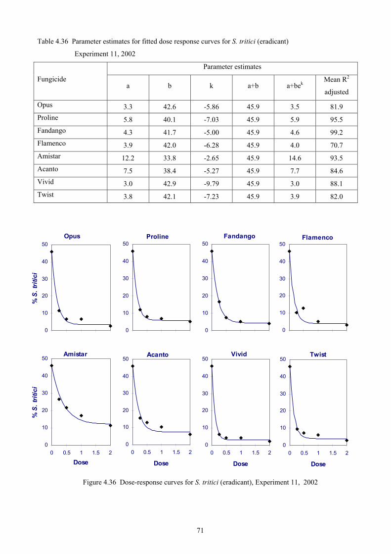
71
Table 4.36 Parameter estimates for fitted dose response curves for S. tritici (eradicant)
Experiment 11, 2002
Parameter estimates
Fungicide a b k a+b a+bek
Mean R2
adjusted
Opus 3.3 42.6 -5.86 45.9 3.5 81.9 Proline 5.8 40.1 -7.03 45.9 5.9 95.5 Fandango 4.3 41.7 -5.00 45.9 4.6 99.2 Flamenco 3.9 42.0 -6.28 45.9 4.0 70.7 Amistar 12.2 33.8 -2.65 45.9 14.6 93.5 Acanto 7.5 38.4 -5.27 45.9 7.7 84.6 Vivid 3.0 42.9 -9.79 45.9 3.0 88.1 Twist 3.8 42.1 -7.23 45.9 3.9 82.0
Figure 4.36 Dose-response curves for S. tritici (eradicant), Experiment 11, 2002
Opus
0
10
20
30
40
50
% S
. tri
tici
Amistar
0
10
20
30
40
50
0 0.5 1 1.5 2
Dose
% S
. tri
tici
Proline
0
10
20
30
40
50Fandango
0
10
20
30
40
50
Acanto
0
10
20
30
40
50
0 0.5 1 1.5 2
Dose
Vivid
0
10
20
30
40
50
0 0.5 1 1.5 2
Dose
Flamenco
0
10
20
30
40
50
Twist
0
10
20
30
40
50
0 0.5 1 1.5 2
Dose
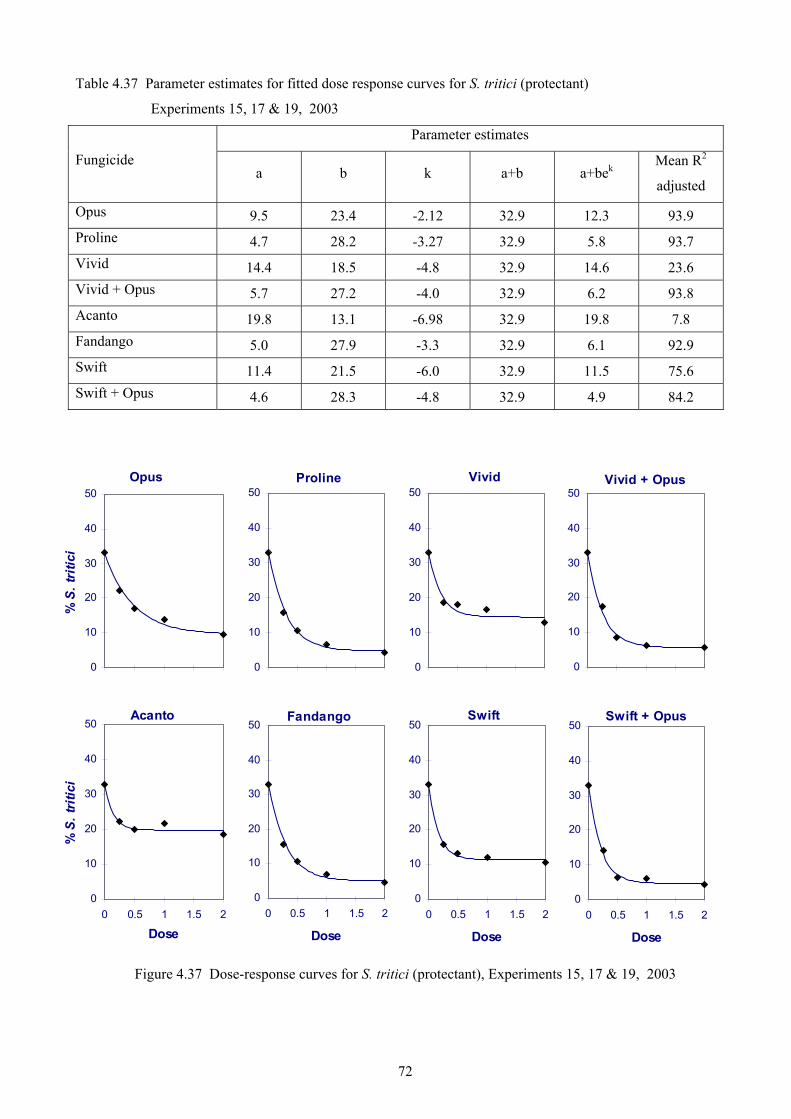
72
Table 4.37 Parameter estimates for fitted dose response curves for S. tritici (protectant)
Experiments 15, 17 & 19, 2003
Parameter estimates
Fungicide a b k a+b a+bek
Mean R2
adjusted
Opus 9.5 23.4 -2.12 32.9 12.3 93.9 Proline 4.7 28.2 -3.27 32.9 5.8 93.7 Vivid 14.4 18.5 -4.8 32.9 14.6 23.6 Vivid + Opus 5.7 27.2 -4.0 32.9 6.2 93.8 Acanto 19.8 13.1 -6.98 32.9 19.8 7.8 Fandango 5.0 27.9 -3.3 32.9 6.1 92.9 Swift 11.4 21.5 -6.0 32.9 11.5 75.6 Swift + Opus 4.6 28.3 -4.8 32.9 4.9 84.2
Figure 4.37 Dose-response curves for S. tritici (protectant), Experiments 15, 17 & 19, 2003
Opus
0
10
20
30
40
50
% S
. tri
tici
Acanto
0
10
20
30
40
50
0 0.5 1 1.5 2
Dose
% S
. tri
tici
Proline
0
10
20
30
40
50Vivid
0
10
20
30
40
50
Fandango
0
10
20
30
40
50
0 0.5 1 1.5 2
Dose
Swift
0
10
20
30
40
50
0 0.5 1 1.5 2
Dose
Vivid + Opus
0
10
20
30
40
50
Swift + Opus
0
10
20
30
40
50
0 0.5 1 1.5 2
Dose

73
Table 4.38 Parameter estimates for fitted dose response curves for S. tritici (eradicant)
Experiments 15, 17 & 19, 2003
Parameter estimates
Fungicide a b k a+b a+bek
Mean R2
adjusted
Opus 8.4 56.7 -2.11 65.2 15.3 91.2 Proline 8.1 57.1 -2.85 65.2 11.4 79.5 Vivid 28.6 36.6 -2.36 65.2 32.1 77.9 Vivid + Opus 4.4 60.8 -3.91 65.2 5.6 97.0 Acanto 45.8 19.4 -2.22 65.2 47.9 74.9 Fandango 12.0 53.2 -3.42 65.2 13.7 87.4 Swift 19.9 45.3 -0.92 65.2 38.0 91.7 Swift + Opus 5.9 59.2 -4.43 65.2 6.6 81.2
Figure 4.38 Dose-response curves for S. tritici (eradicant), Experiments 15, 17 & 19, 2003
Opus
0
10
20
30
40
50
60
70
% S
. tri
tici
Acanto
0
10
20
30
40
50
60
70
0 0.5 1 1.5 2
Dose
% S
. tri
tici
Proline
0
10
20
30
40
50
60
70Vivid
0
10
20
30
40
50
60
70
Fandango
0
10
20
30
40
50
60
70
0 0.5 1 1.5 2
Dose
Swift
0
10
20
30
40
50
60
70
0 0.5 1 1.5 2
Dose
Vivid + Opus
0
10
20
30
40
50
60
70
Swift + Opus
0
10
20
30
40
50
60
70
0 0.5 1 1.5 2
Dose
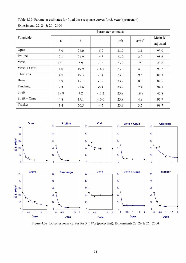
74
Table 4.39 Parameter estimates for fitted dose response curves for S. tritici (protectant)
Experiments 22, 24 & 26, 2004
Parameter estimates
Fungicide a b k a+b a+bek
Mean R2
adjusted
Opus 3.0 21.0 -5.2 23.9 3.1 93.0 Proline 2.1 21.9 -4.8 23.9 2.2 98.6 Vivid 18.1 5.9 -1.6 23.9 19.2 29.6 Vivid + Opus 4.0 19.9 -14.7 23.9 4.0 97.2 Charisma 4.7 19.3 -1.4 23.9 9.5 80.3 Bravo 5.9 18.1 -1.9 23.9 8.5 89.5 Fandango 2.3 21.6 -5.4 23.9 2.4 94.1 Swift 19.8 4.2 -11.2 23.9 19.8 45.8 Swift + Opus 4.8 19.1 -16.0 23.9 4.8 96.7 Tracker 3.4 20.5 -4.5 23.9 3.7 98.7
Figure 4.39 Dose-response curves for S. tritici (protectant), Experiments 22, 24 & 26, 2004
Opus
0
10
20
30
40
50
% S
. tri
tici
Bravo
0
10
20
30
40
50
0 0.5 1 1.5 2
Dose
% S
. tri
tici
Proline
0
10
20
30
40
50Vivid
0
10
20
30
40
50
Fandango
0
10
20
30
40
50
0 0.5 1 1.5 2
Dose
Swift
0
10
20
30
40
50
0 0.5 1 1.5 2
Dose
Vivid + Opus
0
10
20
30
40
50Charisma
0
10
20
30
40
50
Swift + Opus
0
10
20
30
40
50
0 0.5 1 1.5 2
Dose
Tracker
0
10
20
30
40
50
0 0.5 1 1.5 2
Dose

75
Table 4.40 Parameter estimates for fitted dose response curves for S. tritici (eradicant)
Experiments 22, 24 & 26, 2003
Parameter estimates
Fungicide a b k a+b a+bek
Mean R2
adjusted
Opus 8.9 33.2 -2.0 42.1 13.5 96.5 Proline 11.5 30.6 -2.5 42.1 14.0 94.6 Vivid 33.3 8.8 -16.0 42.1 33.3 61.9 Vivid + Opus 15.2 26.9 -16.0 42.1 15.2 95.1 Charisma 15.5 26.6 -1.0 42.1 25.0 92.0 Bravo 23.5 18.7 -3.8 42.1 23.9 93.5 Fandango 9.6 32.5 -2.2 42.1 13.3 99.9 Swift 34.0 8.2 -16.0 42.1 34.0 85.7 Swift + Opus 15.5 26.7 -7.9 42.1 15.5 97.3 Tracker 14.3 27.8 -2.5 42.1 16.6 99.3
Figure 4.40 Dose-response curves for S. tritici (eradicant), Experiments 22, 24 & 26, 2004
Opus
0
10
20
30
40
50
% S
. tri
tici
Bravo
0
10
20
30
40
50
0 0.5 1 1.5 2
Dose
% S
. tri
tici
Proline
0
10
20
30
40
50Vivid
0
10
20
30
40
50
Fandango
0
10
20
30
40
50
0 0.5 1 1.5 2
Dose
Swift
0
10
20
30
40
50
0 0.5 1 1.5 2
Dose
Vivid + Opus
0
10
20
30
40
50Charisma
0
10
20
30
40
50
Swift + Opus
0
10
20
30
40
50
0 0.5 1 1.5 2
Dose
Tracker
0
10
20
30
40
50
0 0.5 1 1.5 2
Dose

76
The contrast in activity of the strobilurin fungicides during the period of the experiments, due to the appearance
of fungicide-resistant strains in the population, is striking. This is illustrated in figures 4.40 and 4.41 which
clearly show the loss of protectant and eradicant activity of Vivid (pyraclostrobin) over the period 2002-2004.
These data clearly show the rapid decline in performance of the strobilurin fungicides against S. tritici during
this period.
2002 2003 2004
Figure 4.41 Dose-response curves for S. tritici (protectant) over period 2002-2004
2002 2003 2004
Figure 4.42 Dose-response curves for S. tritici (eradicant) over period 2002-2004
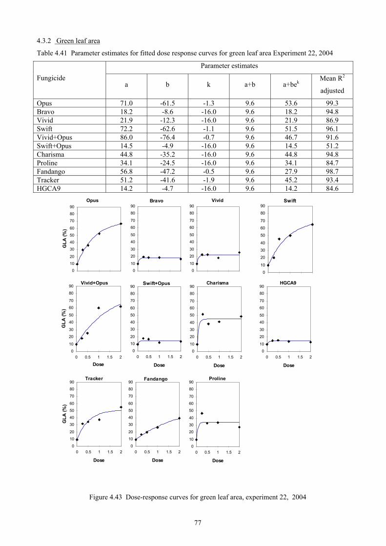
77
4.3.2 Green leaf area
Table 4.41 Parameter estimates for fitted dose response curves for green leaf area Experiment 22, 2004
Parameter estimates
Fungicide a b k a+b a+bek
Mean R2
adjusted
Opus 71.0 -61.5 -1.3 9.6 53.6 99.3 Bravo 18.2 -8.6 -16.0 9.6 18.2 94.8 Vivid 21.9 -12.3 -16.0 9.6 21.9 86.9 Swift 72.2 -62.6 -1.1 9.6 51.5 96.1 Vivid+Opus 86.0 -76.4 -0.7 9.6 46.7 91.6 Swift+Opus 14.5 -4.9 -16.0 9.6 14.5 51.2 Charisma 44.8 -35.2 -16.0 9.6 44.8 94.8 Proline 34.1 -24.5 -16.0 9.6 34.1 84.7 Fandango 56.8 -47.2 -0.5 9.6 27.9 98.7 Tracker 51.2 -41.6 -1.9 9.6 45.2 93.4 HGCA9 14.2 -4.7 -16.0 9.6 14.2 84.6
Figure 4.43 Dose-response curves for green leaf area, experiment 22, 2004
Opus
0
10
20
30
40
50
60
70
80
90
GLA
(%)
Bravo
0
10
20
30
40
50
60
70
80
90Vivid
0
10
20
30
40
50
60
70
80
90
Vivid+Opus
0
10
20
30
40
50
60
70
80
90
0 0.5 1 1.5 2
Dose
GLA
(%)
Swift+Opus
0
10
20
30
40
50
60
70
80
90
0 0.5 1 1.5 2
Dose
Charisma
0
10
20
30
40
50
60
70
80
90
0 0.5 1 1.5 2
Dose
Tracker
0
10
20
30
40
50
60
70
80
90
0 0.5 1 1.5 2
Dose
GLA
(%)
Fandango
0
10
20
30
40
50
60
70
80
90
0 0.5 1 1.5 2
Dose
Proline
0
10
20
30
40
50
60
70
80
90
0 0.5 1 1.5 2
Dose
Swift
0
10
20
30
40
50
60
70
80
90
HGCA9
0
10
20
30
40
50
60
70
80
90
0 0.5 1 1.5 2
Dose

78
Table 4.42 Parameter estimates for fitted dose response curves for green leaf area Experiment 24, 2004
Parameter estimates
Fungicide a b k a+b a+bek
Mean R2
adjusted
Opus 81.1 -26.2 -5.2 54.9 81.0 76.2 Bravo 75.1 -20.2 -16.0 54.9 75.1 71.6 Vivid 73.0 -18.1 -7.6 54.9 73.0 99.4 Swift 95.3 -40.3 -1.8 54.9 88.4 87.1 Vivid+Opus 87.5 -32.6 -3.5 54.9 86.6 92.2 Swift+Opus 71.3 -16.4 -16.0 54.9 71.3 64.5 Charisma 86.1 -31.2 -7.5 54.9 86.1 97.5 Proline 85.4 -30.4 -7.6 54.9 85.3 83.8 Fandango 76.4 -21.5 -3.7 54.9 75.9 71.9 Tracker 84.5 -29.6 -3.8 54.9 83.9 94.1 HGCA9 88.3 -33.3 -0.3 54.9 64.4 13.9
Figure 4.44 Dose-response curves for green leaf area, experiment 24, 2004
Opus
40
50
60
70
80
90
100
GLA
(%)
Bravo
40
50
60
70
80
90
100Vivid
40
50
60
70
80
90
100
Vivid+Opus
40
50
60
70
80
90
100
0 0.5 1 1.5 2
Dose
GLA
(%)
Swift+Opus
40
50
60
70
80
90
100
0 0.5 1 1.5 2
Dose
Charisma
40
50
60
70
80
90
100
0 0.5 1 1.5 2
Dose
Tracker
40
50
60
70
80
90
100
0 0.5 1 1.5 2
Dose
GLA
(%)
Fandango
40
50
60
70
80
90
100
0 0.5 1 1.5 2
Dose
Proline
40
50
60
70
80
90
100
0 0.5 1 1.5 2
Dose
Swift
40
50
60
70
80
90
100
HGCA9
40
50
60
70
80
90
100
0 0.5 1 1.5 2
Dose
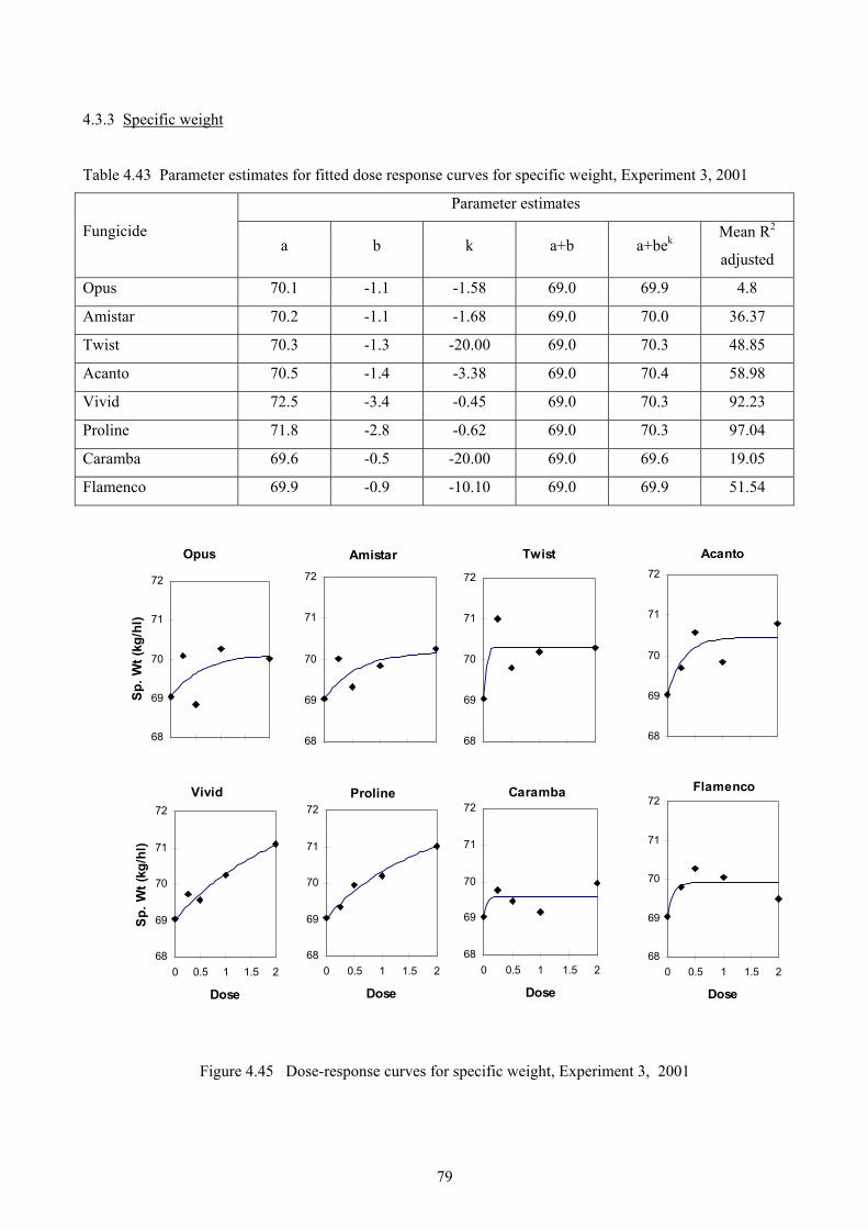
79
4.3.3 Specific weight
Table 4.43 Parameter estimates for fitted dose response curves for specific weight, Experiment 3, 2001
Parameter estimates
Fungicide a b k a+b a+bek
Mean R2
adjusted
Opus 70.1 -1.1 -1.58 69.0 69.9 4.8
Amistar 70.2 -1.1 -1.68 69.0 70.0 36.37
Twist 70.3 -1.3 -20.00 69.0 70.3 48.85
Acanto 70.5 -1.4 -3.38 69.0 70.4 58.98
Vivid 72.5 -3.4 -0.45 69.0 70.3 92.23
Proline 71.8 -2.8 -0.62 69.0 70.3 97.04
Caramba 69.6 -0.5 -20.00 69.0 69.6 19.05
Flamenco 69.9 -0.9 -10.10 69.0 69.9 51.54
Figure 4.45 Dose-response curves for specific weight, Experiment 3, 2001
Opus
68
69
70
71
72
Sp. W
t (kg
/hl)
Vivid
68
69
70
71
72
0 0.5 1 1.5 2
Dose
Sp. W
t (kg
/hl)
Amistar
68
69
70
71
72
Twist
68
69
70
71
72
Proline
68
69
70
71
72
0 0.5 1 1.5 2
Dose
Caramba
68
69
70
71
72
0 0.5 1 1.5 2
Dose
Acanto
68
69
70
71
72
Flamenco
68
69
70
71
72
0 0.5 1 1.5 2
Dose

80
Table 4.44 Parameter estimates for fitted dose response curves for specific weight, Experiment 4, 2001
Parameter estimates
Fungicide a b k a+b a+bek
Mean R2
adjusted
Opus 73.2 -0.5 -4.46 72.7 73.2 -0.6
Amistar 73.0 -0.3 -20.00 72.7 73.0 -50.0
Twist 74.2 -1.5 -0.36 72.7 73.2 82.9
Acanto 73.1 -0.4 -7.74 72.7 73.1 -49.3
Vivid 73.1 -0.4 -1.45 72.7 73.0 -4.2
Proline 73.2 -0.5 -20.00 72.7 73.2 -50.0
Caramba 73.2 -0.5 -5.20 72.7 73.2 -20.4
Flamenco 73.1 -0.4 -20.00 72.7 73.1 -50.0
Figure 4.46 Dose-response curves for specific weight, Experiment 4, 2001
Opus
71
72
73
74
Sp.
Wt (
kg/h
l)
Vivid
71
72
73
74
0 0.5 1 1.5 2
Dose
Sp.
Wt (
kg/h
l)
Amistar
71
72
73
74Twist
71
72
73
74
Proline
71
72
73
74
0 0.5 1 1.5 2
Dose
Caramba
71
72
73
74
0 0.5 1 1.5 2
Dose
Acanto
71
72
73
74
Flamenco
71
72
73
74
0 0.5 1 1.5 2
Dose

81
Table 4.45 Parameter estimates for fitted dose response curves for specific weight, Experiment 15, 2003
Parameter estimates
Fungicide a b k a+b a+bek
Mean R2
adjusted
Opus 75.7 -2.8 -2.71 73.0 75.5 62.2
Proline 75.4 -2.4 -1.71 73.0 74.9 94.8
Acanto 74.3 -1.3 -3.24 73.0 74.2 -40.5
Vivid 74.0 -1.1 -7.65 73.0 74.0 42.0
Fandango 75.4 -2.5 -4.51 73.0 75.4 48.6
Swift 75.4 -2.4 -2.04 73.0 75.1 2.7
Vivid+Opus 76.0 -3.0 -5.52 73.0 75.9 46.8
Swift+Opus 76.3 -3.3 -3.86 73.0 76.2 70.8
Figure 4.47 Dose-response curves for specific weight, Experiment 15, 2003
Opus
72
73
74
75
76
77
Sp
Wt.(
kg/h
l)
Fandango
72
73
74
75
76
77
0 0.5 1 1.5 2
Dose
Sp W
t.(kg
/hl)
Proline
72
73
74
75
76
77Acanto
72
73
74
75
76
77
Swift
72
73
74
75
76
77
0 0.5 1 1.5 2
Dose
Vivid+Opus
72
73
74
75
76
77
0 0.5 1 1.5 2
Dose
Vivid
72
73
74
75
76
77
Swift+Opus
72
73
74
75
76
77
0 0.5 1 1.5 2
Dose
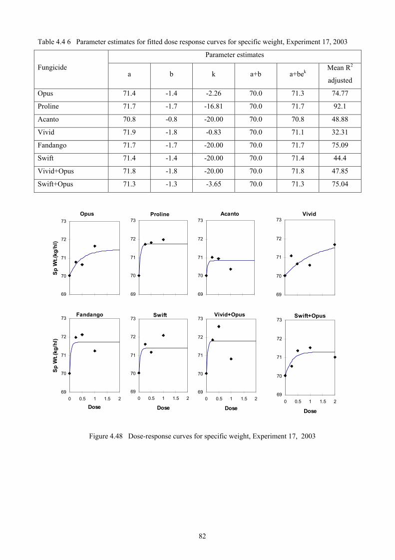
82
Table 4.4 6 Parameter estimates for fitted dose response curves for specific weight, Experiment 17, 2003
Parameter estimates
Fungicide a b k a+b a+bek
Mean R2
adjusted
Opus 71.4 -1.4 -2.26 70.0 71.3 74.77
Proline 71.7 -1.7 -16.81 70.0 71.7 92.1
Acanto 70.8 -0.8 -20.00 70.0 70.8 48.88
Vivid 71.9 -1.8 -0.83 70.0 71.1 32.31
Fandango 71.7 -1.7 -20.00 70.0 71.7 75.09
Swift 71.4 -1.4 -20.00 70.0 71.4 44.4
Vivid+Opus 71.8 -1.8 -20.00 70.0 71.8 47.85
Swift+Opus 71.3 -1.3 -3.65 70.0 71.3 75.04
Figure 4.48 Dose-response curves for specific weight, Experiment 17, 2003
Opus
69
70
71
72
73
Sp
Wt.(
kg/h
l)
Fandango
69
70
71
72
73
0 0.5 1 1.5 2
Dose
Sp W
t.(kg
/hl)
Proline
69
70
71
72
73Acanto
69
70
71
72
73
Swift
69
70
71
72
73
0 0.5 1 1.5 2
Dose
Vivid+Opus
69
70
71
72
73
0 0.5 1 1.5 2
Dose
Vivid
69
70
71
72
73
Swift+Opus
69
70
71
72
73
0 0.5 1 1.5 2
Dose
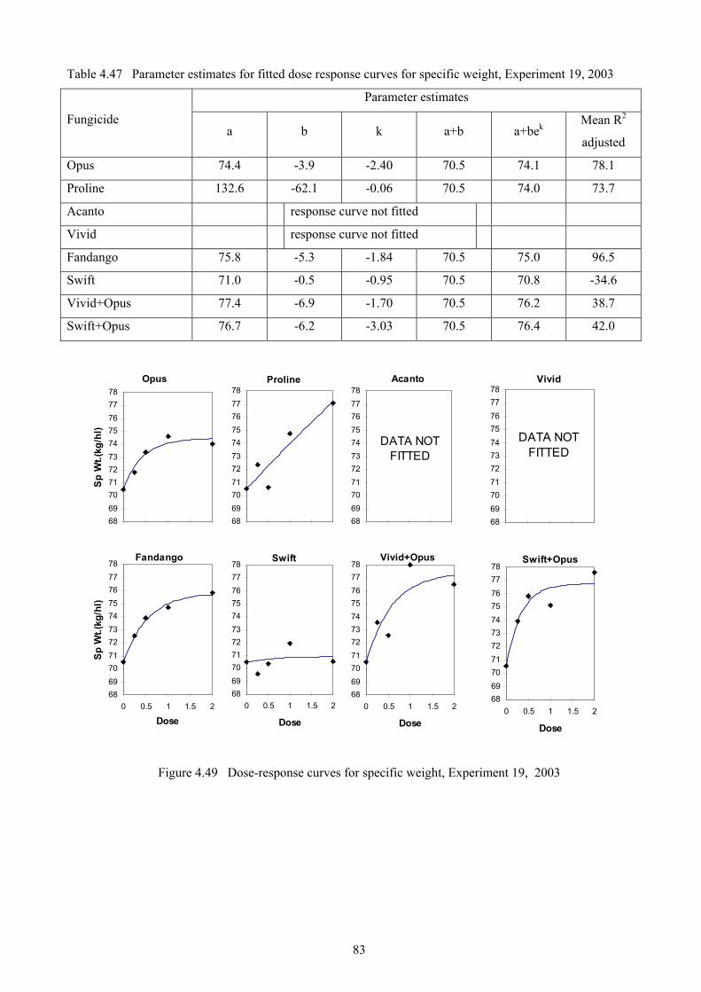
83
Table 4.47 Parameter estimates for fitted dose response curves for specific weight, Experiment 19, 2003
Parameter estimates
Fungicide a b k a+b a+bek
Mean R2
adjusted
Opus 74.4 -3.9 -2.40 70.5 74.1 78.1
Proline 132.6 -62.1 -0.06 70.5 74.0 73.7
Acanto response curve not fitted
Vivid response curve not fitted
Fandango 75.8 -5.3 -1.84 70.5 75.0 96.5
Swift 71.0 -0.5 -0.95 70.5 70.8 -34.6
Vivid+Opus 77.4 -6.9 -1.70 70.5 76.2 38.7
Swift+Opus 76.7 -6.2 -3.03 70.5 76.4 42.0
Figure 4.49 Dose-response curves for specific weight, Experiment 19, 2003
Opus
6869707172737475767778
Sp
Wt.(
kg/h
l)
Fandango
6869707172737475767778
0 0.5 1 1.5 2
Dose
Sp W
t.(kg
/hl)
Proline
6869707172737475767778
Acanto
6869707172737475767778
DATA NOTFITTED
Swift
6869707172737475767778
0 0.5 1 1.5 2
Dose
Vivid+Opus
6869707172737475767778
0 0.5 1 1.5 2
Dose
Vivid
6869707172737475767778
DATA NOTFITTED
Swift+Opus
6869707172737475767778
0 0.5 1 1.5 2
Dose

84
Table 4.48 Parameter estimates for fitted dose response curves for specific weight, Experiment 22, 2004
Parameter estimates
Fungicide a b k a+b a+bek
Mean R2
adjusted
Opus 68.6 -4.0 -2.3 64.6 68.2 87.3 Bravo 67.6 -3.1 -2.8 64.6 67.5 87.9 Vivid 65.6 -1.1 -2.6 64.6 65.6 79.3 Swift 65.6 -1.0 -3.1 64.6 65.5 15.5 Vivid+Opus 67.7 -3.1 -16.0 64.6 67.7 87.0 Swift+Opus 68.1 -3.5 -13.4 64.6 68.1 94.3 Charisma 67.8 -3.2 -2.3 64.6 67.4 92.4 Proline 68.8 -4.3 -2.1 64.6 68.3 78.5 Fandango 68.4 -3.8 -5.9 64.6 68.4 89.6 Tracker 69.1 -4.6 -2.9 64.6 68.9 86.6 HGCA9 66.9 -2.3 -0.5 64.6 65.5 28.2
Figure 4.50 Dose-response curves for specific weight, Experiment 22, 2004
Opus
64
65
66
67
68
69
70
Sp W
t.(kg
/hl)
Bravo
64
65
66
67
68
69
70Vivid
64
65
66
67
68
69
70Swift
64
65
66
67
68
69
70
Vivid+Opus
64
65
66
67
68
69
70
0 0.5 1 1.5 2
Dose
Sp W
t.(kg
/hl)
Swift+Opus
64
65
66
67
68
69
70
0 0.5 1 1.5 2
Dose
Charisma
64
65
66
67
68
69
70
0 0.5 1 1.5 2
Dose
Tracker
64
65
66
67
68
69
70
0 0.5 1 1.5 2
Dose
Sp.
Wt.(
kg/h
l)
Fandango
64
65
66
67
68
69
70
0 0.5 1 1.5 2
Dose
Proline
64
65
66
67
68
69
70
0 0.5 1 1.5 2
Dose
HGCA9
64
65
66
67
68
69
70
0 0.5 1 1.5 2
Dose

85
Table 4.49 Parameter estimates for fitted dose response curves for specific weight, Experiment 24, 2004
Parameter estimates
Fungicide a b k a+b a+bek
Mean R2
adjusted
Opus 68.9 -1.0 -0.7 67.9 68.4 13.8 Bravo 67.9 0.0 16.0 67.9 67.9 25.6 Vivid 69.0 -1.1 0.2 67.9 67.7 -91.9 Swift 67.4 0.5 -16.0 67.9 67.4 77 Vivid+Opus 68.8 -0.8 -4.1 67.9 68.8 58.2 Swift+Opus 68.3 -0.3 -16.0 67.9 68.3 47.1 Charisma 67.9 0.0 0.7 67.9 68.0 -31.1 Proline 68.4 -0.4 -16.0 67.9 68.4 -26.8 Fandango 70.1 -2.1 -0.3 67.9 68.5 72.9 Tracker 70.3 -2.4 0.1 67.9 67.7 -27.5 HGCA9 68.3 -0.4 0.1 67.9 67.9 -63.1
Figure 4.51 Dose-response curves for specific weight, Experiment 24, 2004
Opus
64
65
66
67
68
69
70
Sp
Wt.(
kg/h
l)
Bravo
64
65
66
67
68
69
70Vivid
64
65
66
67
68
69
70
Vivid+Opus
64
65
66
67
68
69
70
0 0.5 1 1.5 2
Dose
Sp W
t.(kg
/hl)
Swift+Opus
64
65
66
67
68
69
70
0 0.5 1 1.5 2
Dose
Charisma
64
65
66
67
68
69
70
0 0.5 1 1.5 2
Dose
Tracker
64
65
66
67
68
69
70
0 0.5 1 1.5 2
Dose
Sp. W
t.(kg
/hl)
Fandango
64
65
66
67
68
69
70
0 0.5 1 1.5 2
Dose
Proline
64
65
66
67
68
69
70
0 0.5 1 1.5 2
Dose
Swift
64
65
66
67
68
69
70
HGCA9
64
65
66
67
68
69
70
0 0.5 1 1.5 2
Dose
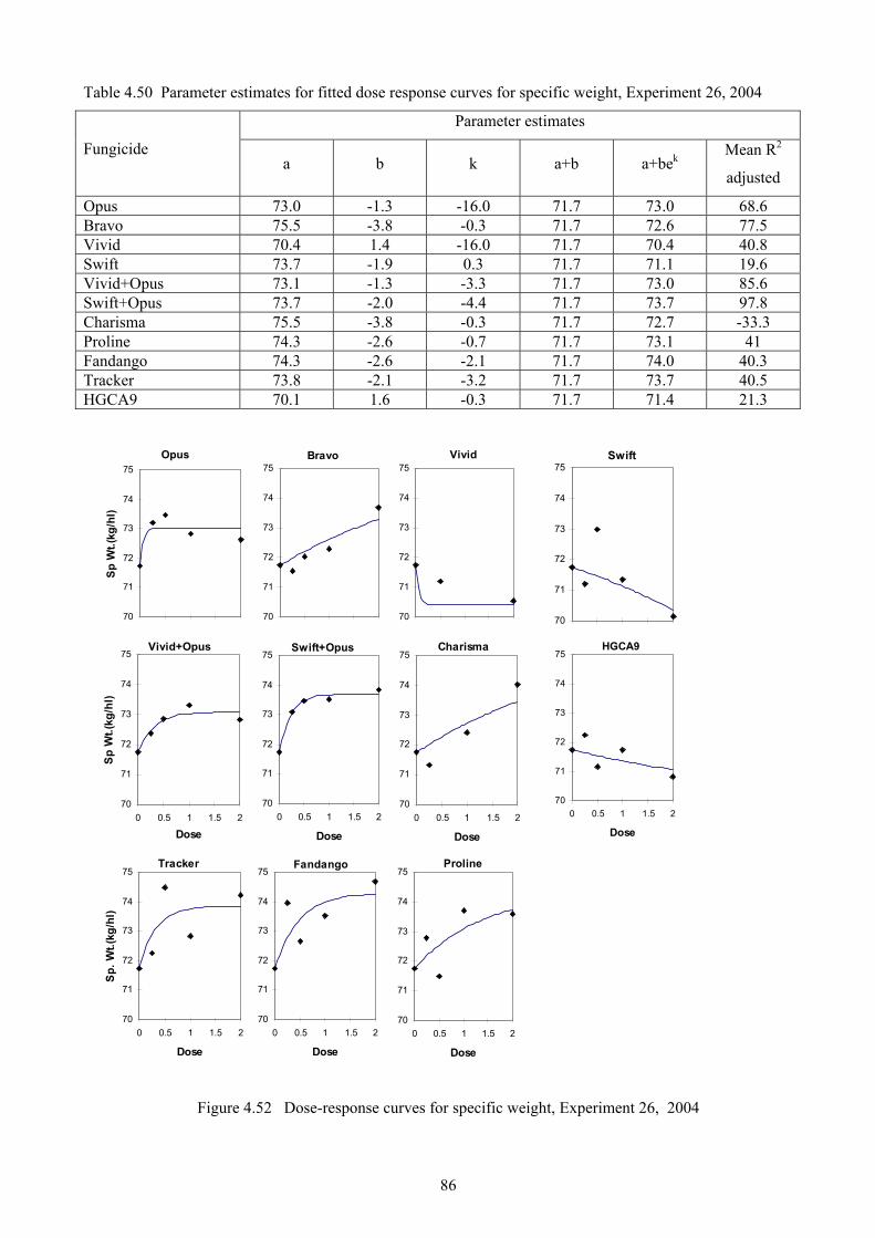
86
Table 4.50 Parameter estimates for fitted dose response curves for specific weight, Experiment 26, 2004
Parameter estimates
Fungicide a b k a+b a+bek
Mean R2
adjusted
Opus 73.0 -1.3 -16.0 71.7 73.0 68.6 Bravo 75.5 -3.8 -0.3 71.7 72.6 77.5 Vivid 70.4 1.4 -16.0 71.7 70.4 40.8 Swift 73.7 -1.9 0.3 71.7 71.1 19.6 Vivid+Opus 73.1 -1.3 -3.3 71.7 73.0 85.6 Swift+Opus 73.7 -2.0 -4.4 71.7 73.7 97.8 Charisma 75.5 -3.8 -0.3 71.7 72.7 -33.3 Proline 74.3 -2.6 -0.7 71.7 73.1 41 Fandango 74.3 -2.6 -2.1 71.7 74.0 40.3 Tracker 73.8 -2.1 -3.2 71.7 73.7 40.5 HGCA9 70.1 1.6 -0.3 71.7 71.4 21.3
Figure 4.52 Dose-response curves for specific weight, Experiment 26, 2004
Opus
70
71
72
73
74
75
Sp
Wt.(
kg/h
l)
Bravo
70
71
72
73
74
75Vivid
70
71
72
73
74
75
Vivid+Opus
70
71
72
73
74
75
0 0.5 1 1.5 2
Dose
Sp
Wt.(
kg/h
l)
Swift+Opus
70
71
72
73
74
75
0 0.5 1 1.5 2
Dose
Charisma
70
71
72
73
74
75
0 0.5 1 1.5 2
Dose
Tracker
70
71
72
73
74
75
0 0.5 1 1.5 2
Dose
Sp. W
t.(kg
/hl)
Fandango
70
71
72
73
74
75
0 0.5 1 1.5 2
Dose
Proline
70
71
72
73
74
75
0 0.5 1 1.5 2
Dose
Swift
70
71
72
73
74
75
HGCA9
70
71
72
73
74
75
0 0.5 1 1.5 2
Dose

87
4.3.4 Yield
Table 4.51 Parameter estimates for fitted dose response curves for yield, Experiment 4, 2001
Parameter estimates
Fungicide a b k a+b a+bek
Mean R2
adjusted
Opus 9.9 -0.8 -3.33 9.1 9.9 10.0
Amistar 9.8 -0.7 -2.26 9.1 9.8 17.5
Twist 9.7 -0.6 -20.00 9.1 9.7 -50.0
Acanto 10.3 -1.2 -2.70 9.1 10.2 77.8
Vivid 10.1 -1.0 -6.02 9.1 10.1 88.9
Proline 10.4 -1.3 -1.42 9.1 10.1 37.8
Caramba 9.9 -0.8 -19.45 9.1 9.9 -50.0
Flamenco 9.8 -0.7 -1.50 9.1 9.6 60.6
Figure 4.53 Dose-response curves for yield, Experiment 4, 2001
Opus
8
9
10
11
Yie
ld t/
ha
Vivid
8
9
10
11
0 0.5 1 1.5 2
Dose
Yie
ld t/
ha
Amistar
8
9
10
11
Twist
8
9
10
11
Proline
8
9
10
11
0 0.5 1 1.5 2
Dose
Caramba
8
9
10
11
0 0.5 1 1.5 2
Dose
Acanto
8
9
10
11
Flamenco
8
9
10
11
0 0.5 1 1.5 2
Dose
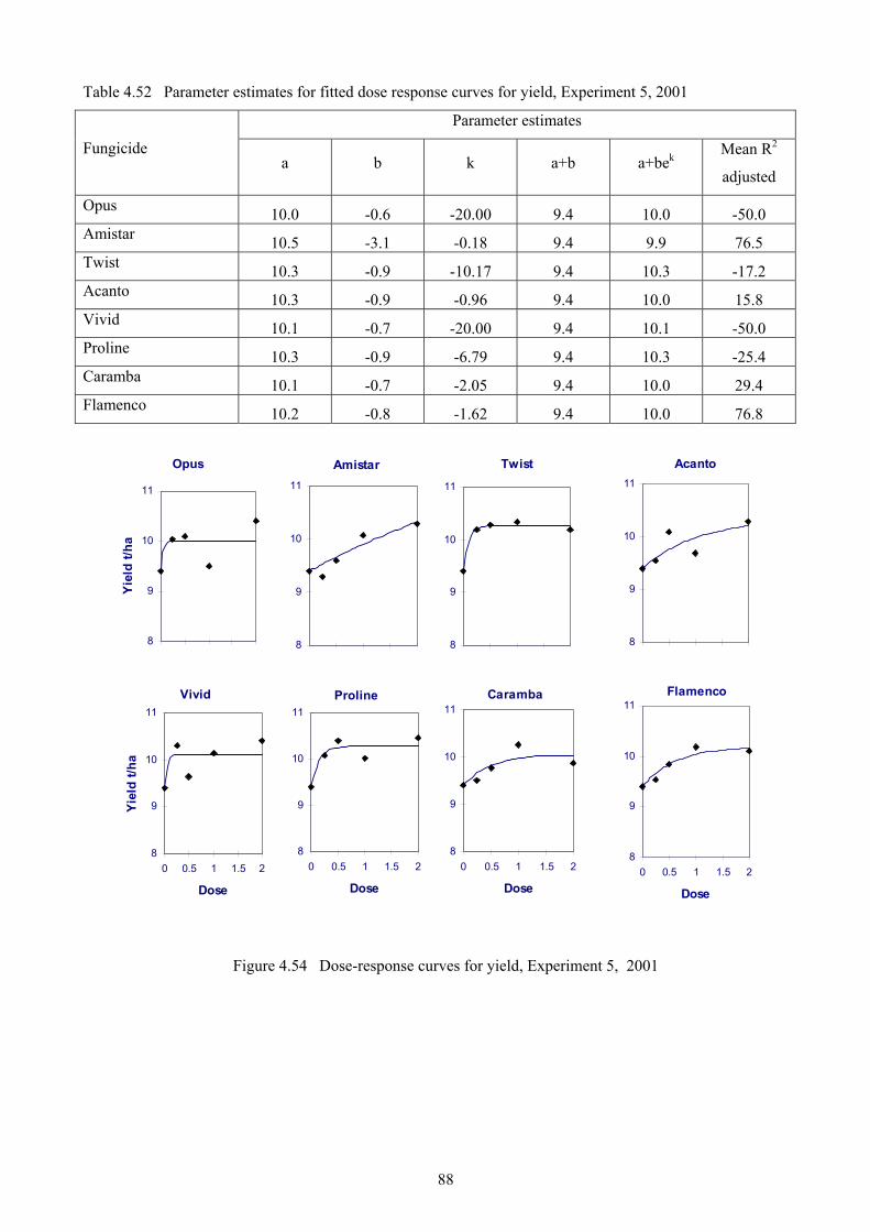
88
Table 4.52 Parameter estimates for fitted dose response curves for yield, Experiment 5, 2001
Parameter estimates
Fungicide a b k a+b a+bek
Mean R2
adjusted
Opus 10.0 -0.6 -20.00 9.4 10.0 -50.0 Amistar 10.5 -3.1 -0.18 9.4 9.9 76.5 Twist 10.3 -0.9 -10.17 9.4 10.3 -17.2 Acanto 10.3 -0.9 -0.96 9.4 10.0 15.8 Vivid 10.1 -0.7 -20.00 9.4 10.1 -50.0 Proline 10.3 -0.9 -6.79 9.4 10.3 -25.4 Caramba 10.1 -0.7 -2.05 9.4 10.0 29.4 Flamenco 10.2 -0.8 -1.62 9.4 10.0 76.8
Figure 4.54 Dose-response curves for yield, Experiment 5, 2001
Acanto
8
9
10
11
Flamenco
8
9
10
11
0 0.5 1 1.5 2
Dose
Opus
8
9
10
11
Yie
ld t/
ha
Vivid
8
9
10
11
0 0.5 1 1.5 2
Dose
Yiel
d t/h
a
Amistar
8
9
10
11
Twist
8
9
10
11
Proline
8
9
10
11
0 0.5 1 1.5 2
Dose
Caramba
8
9
10
11
0 0.5 1 1.5 2
Dose
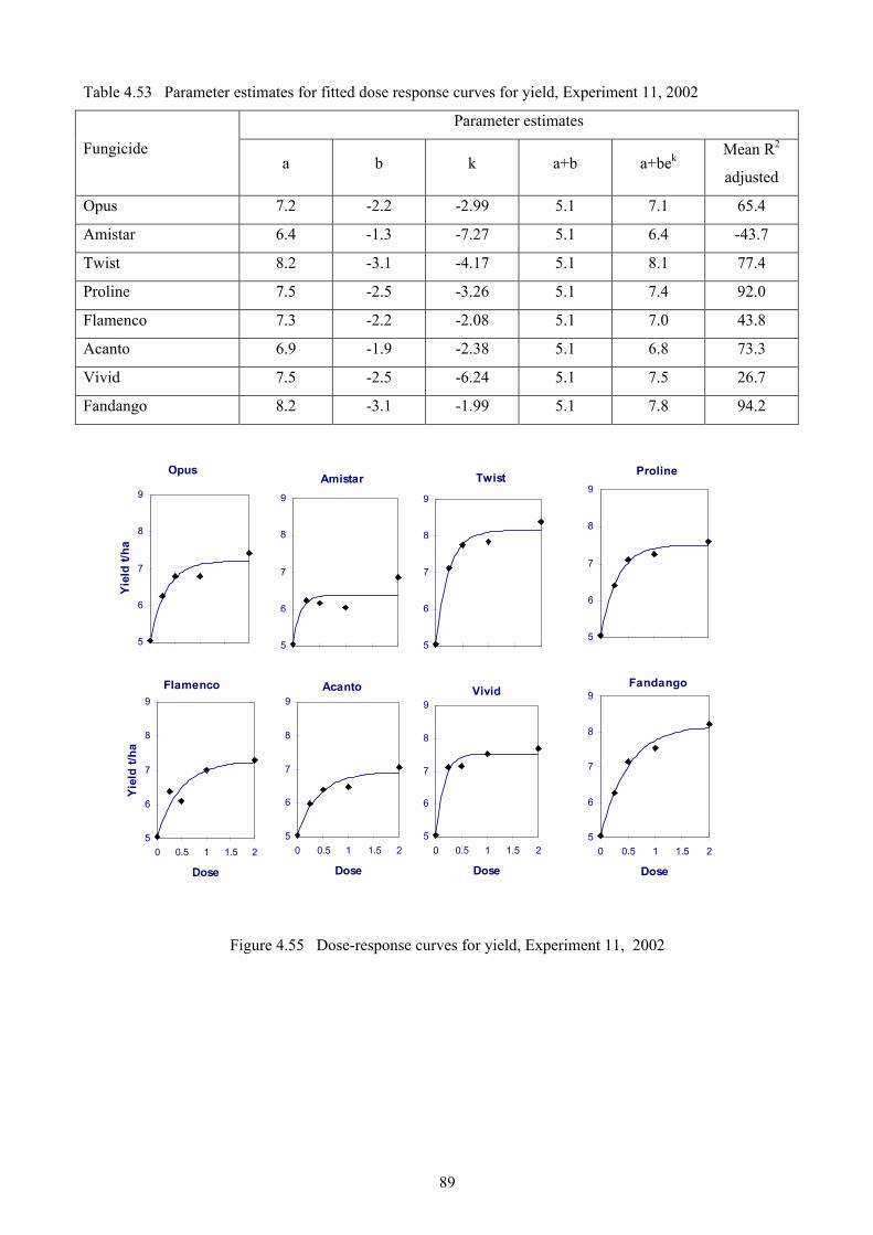
89
Table 4.53 Parameter estimates for fitted dose response curves for yield, Experiment 11, 2002
Parameter estimates
Fungicide a b k a+b a+bek
Mean R2
adjusted
Opus 7.2 -2.2 -2.99 5.1 7.1 65.4
Amistar 6.4 -1.3 -7.27 5.1 6.4 -43.7
Twist 8.2 -3.1 -4.17 5.1 8.1 77.4
Proline 7.5 -2.5 -3.26 5.1 7.4 92.0
Flamenco 7.3 -2.2 -2.08 5.1 7.0 43.8
Acanto 6.9 -1.9 -2.38 5.1 6.8 73.3
Vivid 7.5 -2.5 -6.24 5.1 7.5 26.7
Fandango 8.2 -3.1 -1.99 5.1 7.8 94.2
Figure 4.55 Dose-response curves for yield, Experiment 11, 2002
Opus
5
6
7
8
9
Yiel
d t/h
a
Flamenco
5
6
7
8
9
0 0.5 1 1.5 2
Dose
Yiel
d t/h
a
Amistar
5
6
7
8
9
Twist
5
6
7
8
9
Acanto
5
6
7
8
9
0 0.5 1 1.5 2
Dose
Vivid
5
6
7
8
9
0 0.5 1 1.5 2
Dose
Proline
5
6
7
8
9
Fandango
5
6
7
8
9
0 0.5 1 1.5 2
Dose

90
Table 4.54 Parameter estimates for fitted dose response curves for yield, Experiment 15, 2003
Parameter estimates
Fungicide a b k a+b a+bek
Mean R2
adjusted
Opus 10.0 -1.1 -2.52 8.9 9.9 99.2
Proline 10.1 -1.2 -1.79 8.9 9.9 97.3
Acanto 9.5 -0.6 -3.06 8.9 9.5 89.3
Vivid 9.6 -0.7 -3.54 8.9 9.6 45.5
Fandango 10.3 -1.4 -2.11 8.9 10.2 86.3
Swift 9.6 -0.6 -20.00 8.9 9.6 -50.0
Vivid+Opus 10.3 -1.4 -3.99 8.9 10.3 77.3
Swift+Opus 10.5 -1.6 -2.95 8.9 10.5 88.0
Figure 4.56 Dose-response curves for yield, Experiment 15, 2003
Opus
8
9
10
11
Yie
ld t/
ha
Fandango
8
9
10
11
0 0.5 1 1.5 2
Dose
Yie
ld t/
ha
Proline
8
9
10
11
Swift
8
9
10
11
0 0.5 1 1.5 2
Dose
Vivid+Opus
8
9
10
11
0 0.5 1 1.5 2
Dose
Acanto
8
9
10
11
Swift+Opus
8
9
10
11
0 0.5 1 1.5 2
Dose
Vivid
8
9
10
11
0 0.5 1 1.5 2

91
Table 4.55 Parameter estimates for fitted dose response curves for yield, Experiment 17, 2003
Parameter estimates
Fungicide a b k a+b a+bek
Mean R2
adjusted
Opus 9.4 -0.8 -2.64 8.7 9.4 65.86
Proline 9.9 -1.2 -4.68 8.7 9.8 87.16
Acanto 9.0 -0.4 -2.85 8.7 9.0 7.91
Vivid 9.4 -0.7 -3.16 8.7 9.3 65.87
Fandango 9.9 -1.2 -2.65 8.7 9.8 84.04
Swift 9.5 -0.8 -20.00 8.7 9.5 33.91
Vivid+Opus 9.5 -0.9 -9.37 8.7 9.5 93.75
Swift+Opus 10.1 -1.4 -1.62 8.7 9.8 88.53
Figure 4.57 Dose-response curves for yield, Experiment 17, 2003
Opus
8
9
10
11
Yie
ld t/
ha
Fandango
8
9
10
11
0 0.5 1 1.5 2
Dose
Yie
ld t/
ha
Proline
8
9
10
11
Swift
8
9
10
11
0 0.5 1 1.5 2
Dose
Vivid+Opus
8
9
10
11
0 0.5 1 1.5 2
Dose
Acanto
8
9
10
11
Swift+Opus
8
9
10
11
0 0.5 1 1.5 2
Dose
Vivid
8
9
10
11
0 0.5 1 1.5 2
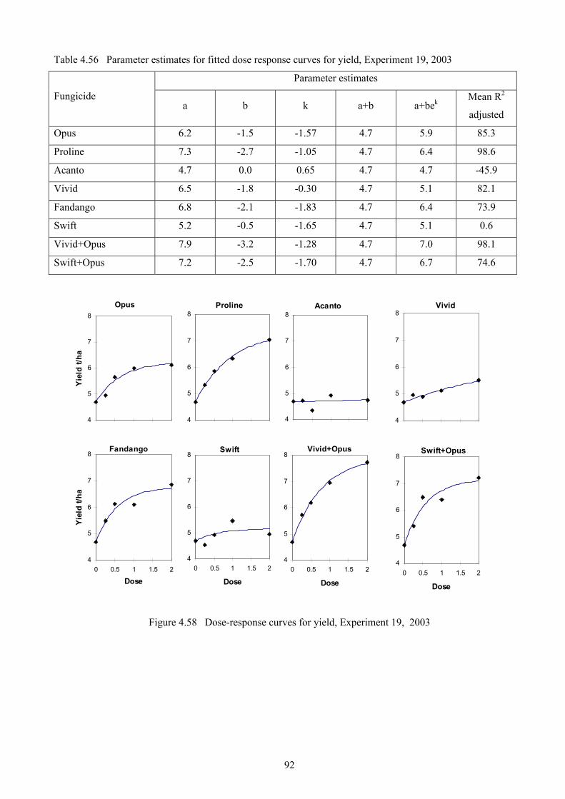
92
Table 4.56 Parameter estimates for fitted dose response curves for yield, Experiment 19, 2003
Parameter estimates
Fungicide a b k a+b a+bek
Mean R2
adjusted
Opus 6.2 -1.5 -1.57 4.7 5.9 85.3
Proline 7.3 -2.7 -1.05 4.7 6.4 98.6
Acanto 4.7 0.0 0.65 4.7 4.7 -45.9
Vivid 6.5 -1.8 -0.30 4.7 5.1 82.1
Fandango 6.8 -2.1 -1.83 4.7 6.4 73.9
Swift 5.2 -0.5 -1.65 4.7 5.1 0.6
Vivid+Opus 7.9 -3.2 -1.28 4.7 7.0 98.1
Swift+Opus 7.2 -2.5 -1.70 4.7 6.7 74.6
Figure 4.58 Dose-response curves for yield, Experiment 19, 2003
Opus
4
5
6
7
8
Yie
ld t/
ha
Fandango
4
5
6
7
8
0 0.5 1 1.5 2
Dose
Yie
ld t/
ha
Proline
4
5
6
7
8
Swift
4
5
6
7
8
0 0.5 1 1.5 2
Dose
Vivid+Opus
4
5
6
7
8
0 0.5 1 1.5 2
Dose
Acanto
4
5
6
7
8
Swift+Opus
4
5
6
7
8
0 0.5 1 1.5 2
Dose
Vivid
4
5
6
7
8
0 0.5 1 1.5 2

93
Table 4.57 Parameter estimates for fitted dose response curves for yield, Experiment 22, 2004
Parameter estimates
Fungicide a b k a+b a+bek
Mean R2
adjusted
Opus 10.1 -2.3 -1.9 7.8 9.7 98.6 Bravo 9.1 -1.3 -0.5 7.8 8.3 95.5 Vivid 8.5 -0.7 -0.2 7.8 7.9 55.9 Swift 7.9 -0.1 -0.1 7.8 7.8 -56.9 Vivid+Opus 9.4 -1.6 -16.0 7.8 9.4 96.5 Swift+Opus 9.4 -1.6 -12.8 7.8 9.4 99.3 Charisma 9.5 -1.7 -0.7 7.8 8.6 99.4 Proline 10.1 -2.3 -2.3 7.8 9.8 97.6 Fandango 10.6 -2.8 -1.2 7.8 9.8 87.2 Tracker 10.0 -2.3 -2.7 7.8 9.9 96.7 HGCA9 9.0 -1.2 -0.2 7.8 8.0 16.3
Figure 4.59 Dose-response curves for yield, Experiment 22, 2004
HGCA9
7
8
9
10
11Opus
7
8
9
10
11
Yie
ld t/
ha
Bravo
7
8
9
10
11Vivid
7
8
9
10
11
Tracker
7
8
9
10
11
0 0.5 1 1.5 2
Dose
Yiel
d t/h
a
Fandango
7
8
9
10
11
0 0.5 1 1.5 2
Dose
Proline
7
8
9
10
11
0 0.5 1 1.5 2
Dose
Vivid+Opus
7
8
9
10
11
0 0.5 1 1.5 2
Dose
Yie
ld t/
ha
Swift+Opus
7
8
9
10
11
0 0.5 1 1.5 2
Dose
Charisma
7
8
9
10
11
0 0.5 1 1.5 2
Dose
Swift
7
8
9
10
11
0 0.5 1 1.5 2
Dose
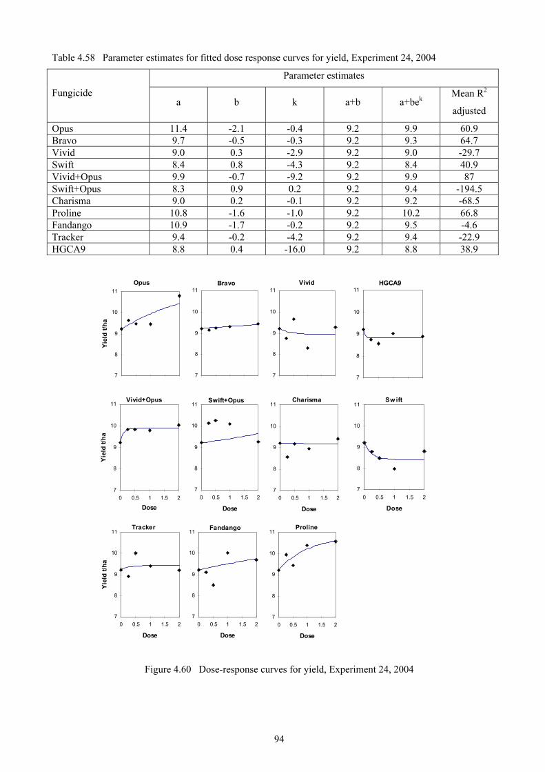
94
Table 4.58 Parameter estimates for fitted dose response curves for yield, Experiment 24, 2004
Parameter estimates
Fungicide a b k a+b a+bek
Mean R2
adjusted
Opus 11.4 -2.1 -0.4 9.2 9.9 60.9 Bravo 9.7 -0.5 -0.3 9.2 9.3 64.7 Vivid 9.0 0.3 -2.9 9.2 9.0 -29.7 Swift 8.4 0.8 -4.3 9.2 8.4 40.9 Vivid+Opus 9.9 -0.7 -9.2 9.2 9.9 87 Swift+Opus 8.3 0.9 0.2 9.2 9.4 -194.5 Charisma 9.0 0.2 -0.1 9.2 9.2 -68.5 Proline 10.8 -1.6 -1.0 9.2 10.2 66.8 Fandango 10.9 -1.7 -0.2 9.2 9.5 -4.6 Tracker 9.4 -0.2 -4.2 9.2 9.4 -22.9 HGCA9 8.8 0.4 -16.0 9.2 8.8 38.9
Figure 4.60 Dose-response curves for yield, Experiment 24, 2004
Opus
7
8
9
10
11
Yiel
d t/h
a
Bravo
7
8
9
10
11Vivid
7
8
9
10
11
Vivid+Opus
7
8
9
10
11
0 0.5 1 1.5 2
Dose
Yie
ld t/
ha
Swift+Opus
7
8
9
10
11
0 0.5 1 1.5 2
Dose
Charisma
7
8
9
10
11
0 0.5 1 1.5 2
Dose
Tracker
7
8
9
10
11
0 0.5 1 1.5 2
Dose
Yiel
d t/h
a
Fandango
7
8
9
10
11
0 0.5 1 1.5 2
Dose
Proline
7
8
9
10
11
0 0.5 1 1.5 2
Dose
HGCA9
7
8
9
10
11
Sw ift
7
8
9
10
11
0 0.5 1 1.5 2
Dose
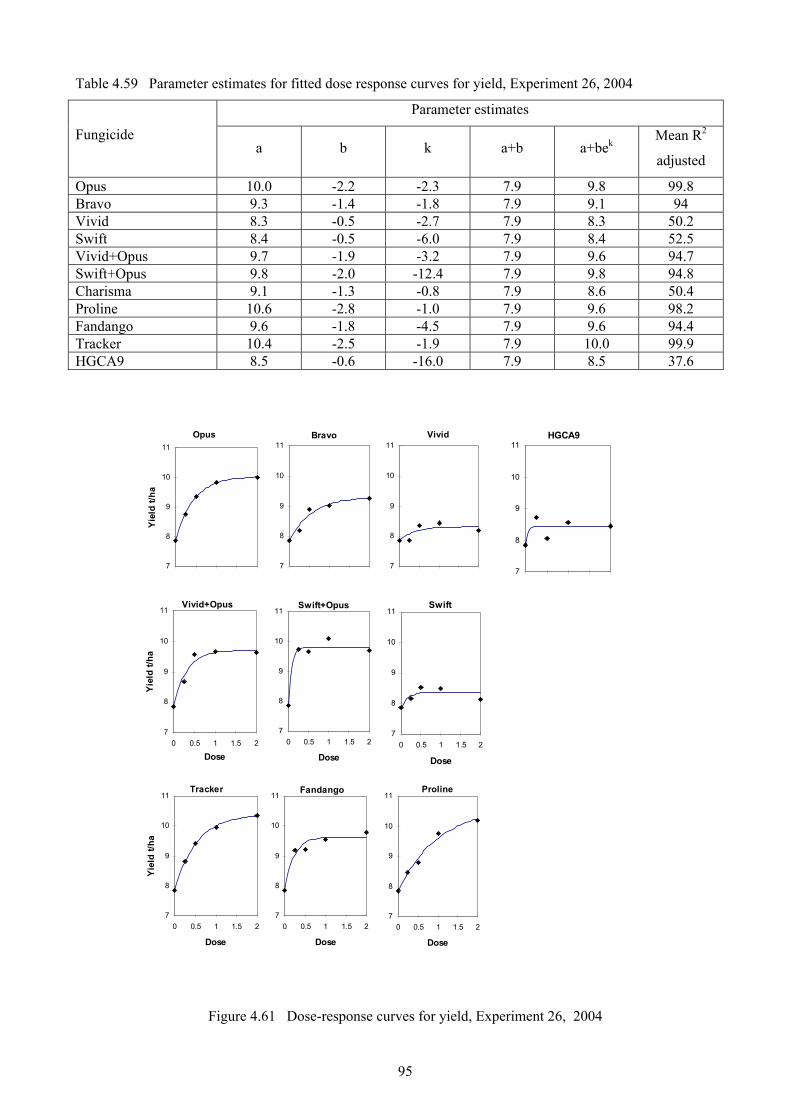
95
Table 4.59 Parameter estimates for fitted dose response curves for yield, Experiment 26, 2004
Parameter estimates
Fungicide a b k a+b a+bek
Mean R2
adjusted
Opus 10.0 -2.2 -2.3 7.9 9.8 99.8 Bravo 9.3 -1.4 -1.8 7.9 9.1 94 Vivid 8.3 -0.5 -2.7 7.9 8.3 50.2 Swift 8.4 -0.5 -6.0 7.9 8.4 52.5 Vivid+Opus 9.7 -1.9 -3.2 7.9 9.6 94.7 Swift+Opus 9.8 -2.0 -12.4 7.9 9.8 94.8 Charisma 9.1 -1.3 -0.8 7.9 8.6 50.4 Proline 10.6 -2.8 -1.0 7.9 9.6 98.2 Fandango 9.6 -1.8 -4.5 7.9 9.6 94.4 Tracker 10.4 -2.5 -1.9 7.9 10.0 99.9 HGCA9 8.5 -0.6 -16.0 7.9 8.5 37.6
Figure 4.61 Dose-response curves for yield, Experiment 26, 2004
Opus
7
8
9
10
11
Yie
ld t/
ha
Bravo
7
8
9
10
11Vivid
7
8
9
10
11
Vivid+Opus
7
8
9
10
11
0 0.5 1 1.5 2
Dose
Yiel
d t/h
a
Swift+Opus
7
8
9
10
11
0 0.5 1 1.5 2
Dose
Charisma
7
8
9
10
11
0 0.5 1 1.5 2
Dose
Tracker
7
8
9
10
11
0 0.5 1 1.5 2
Dose
Yiel
d t/h
a
Fandango
7
8
9
10
11
0 0.5 1 1.5 2
Dose
Proline
7
8
9
10
11
0 0.5 1 1.5 2
Dose
HGCA9
7
8
9
10
11
Swift
7
8
9
10
11
0 0.5 1 1.5 2
Dose
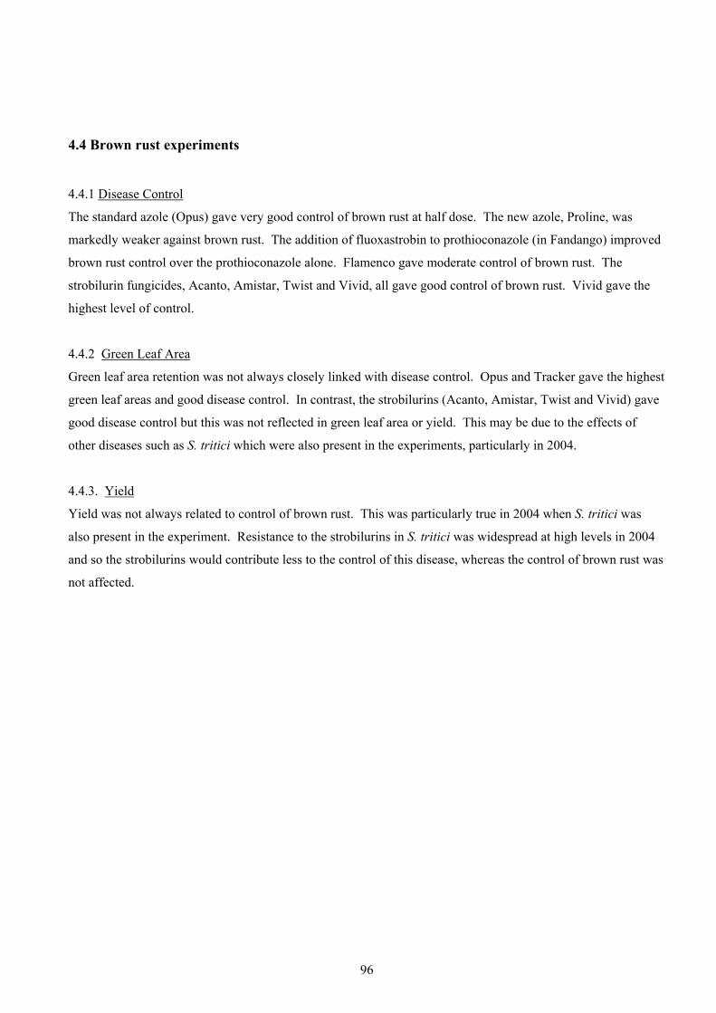
96
4.4 Brown rust experiments
4.4.1 Disease Control
The standard azole (Opus) gave very good control of brown rust at half dose. The new azole, Proline, was
markedly weaker against brown rust. The addition of fluoxastrobin to prothioconazole (in Fandango) improved
brown rust control over the prothioconazole alone. Flamenco gave moderate control of brown rust. The
strobilurin fungicides, Acanto, Amistar, Twist and Vivid, all gave good control of brown rust. Vivid gave the
highest level of control.
4.4.2 Green Leaf Area
Green leaf area retention was not always closely linked with disease control. Opus and Tracker gave the highest
green leaf areas and good disease control. In contrast, the strobilurins (Acanto, Amistar, Twist and Vivid) gave
good disease control but this was not reflected in green leaf area or yield. This may be due to the effects of
other diseases such as S. tritici which were also present in the experiments, particularly in 2004.
4.4.3. Yield
Yield was not always related to control of brown rust. This was particularly true in 2004 when S. tritici was
also present in the experiment. Resistance to the strobilurins in S. tritici was widespread at high levels in 2004
and so the strobilurins would contribute less to the control of this disease, whereas the control of brown rust was
not affected.
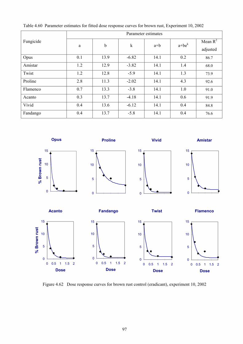
97
Table 4.60 Parameter estimates for fitted dose response curves for brown rust, Experiment 10, 2002
Parameter estimates
Fungicide a b k a+b a+bek
Mean R2
adjusted
Opus 0.1 13.9 -6.82 14.1 0.2 86.7
Amistar 1.2 12.9 -3.82 14.1 1.4 68.0
Twist 1.2 12.8 -5.9 14.1 1.3 73.9
Proline 2.8 11.3 -2.02 14.1 4.3 92.6
Flamenco 0.7 13.3 -3.8 14.1 1.0 91.0
Acanto 0.3 13.7 -4.18 14.1 0.6 91.9
Vivid 0.4 13.6 -6.12 14.1 0.4 84.8
Fandango 0.4 13.7 -5.8 14.1 0.4 76.6
Opus
0
5
10
15
% B
row
n ru
st
Proline
0
5
10
15
Vivid
0
5
10
15
Amistar
0
5
10
15
Acanto
0
5
10
15
0 0.5 1 1.5 2
Dose
% B
row
n ru
st
Fandango
0
5
10
15
0 0.5 1 1.5 2
Dose
Twist
0
5
10
15
0 0.5 1 1.5 2
Dose
Flamenco
0
5
10
15
0 0.5 1 1.5 2
Dose
Figure 4.62 Dose response curves for brown rust control (eradicant), experiment 10, 2002

98
Table 4.61 Parameter estimates for fitted dose response curves for brown rust, Experiment 10, 2002
Parameter estimates
Fungicide a b k a+b a+bek
Mean R2
adjusted
Opus 4.4 26.3 -4.15 30.7 4.8 72
Amistar 4.0 26.7 -1.63 30.7 9.2 60
Twist 4.7 26.0 -1.27 30.7 12.0 74
Proline 13.7 17.0 -1.91 30.7 16.2 51
Flamenco 4.5 26.2 -1.77 30.7 8.9 98
Acanto 1.9 28.8 -1.69 30.7 7.2 97
Vivid 4.7 26.0 -3.48 30.7 5.5 75
Fandango 5.5 25.2 -2.93 30.7 6.8 75
Figure 4.63 Dose response curves for brown rust control (protectant), experiment 10, 2002
Opus
0
5
10
15
20
25
30
35
% B
row
n ru
st
Flamenco
0
5
10
15
20
25
30
35
0 0.5 1 1.5 2
Dose
% B
row
n ru
st
Amistar
0
5
10
15
20
25
30
35
Twist
0
5
10
15
20
25
30
35
Acanto
0
5
10
15
20
25
30
35
0 0.5 1 1.5 2
Dose
Vivid
0
5
10
15
20
25
30
35
0 0.5 1 1.5 2
Dose
Proline
0
5
10
15
20
25
30
35
Fandango
0
5
10
15
20
25
30
35
0 0.5 1 1.5 2
Dose

99
Table 4.62 Parameter estimates for fitted dose response curves for yield, Experiment 10, 2002
Parameter estimates
Fungicide a b k a+b a+bek
Mean R2
adjusted
Opus 8.2 -1.8 -3.74 6.4 8.2 84.87
Amistar 8.0 -1.5 -4.15 6.4 7.9 95.45
Twist 8.1 -1.7 -4.35 6.4 8.0 98.38
Proline 8.2 -1.7 -0.56 6.4 7.2 55.77
Flamenco 7.4 -1.0 -3.49 6.4 7.4 71.74
Acanto 7.8 -1.4 -7.59 6.4 7.8 91.85
Vivid 8.3 -1.9 -5.47 6.4 8.3 94.77
Fandango 8.1 -1.6 -4.51 6.4 8.0 86.80
Figure 4.64 Dose response curves for yield, experiment 10, 2002
Opus
6
7
8
9
Yiel
d t/h
a
Flamenco
6
7
8
9
0 0.5 1 1.5 2
Dose
Yiel
d t/h
a
Amistar
6
7
8
9
Twist
6
7
8
9
Acanto
6
7
8
9
0 0.5 1 1.5 2
Dose
Vivid
6
7
8
9
0 0.5 1 1.5 2
Dose
Proline
6
7
8
9
Fandango
6
7
8
9
0 0.5 1 1.5 2
Dose

100
Table 4.63 Parameter estimates for fitted dose response curves for specific weight, Experiment 10, 2002
Parameter estimates
Fungicide a b k a+b a+bek
Mean R2
adjusted
Opus 77.5 -2.4 -3.82 75.2 77.5 89.7
Amistar 77.6 -2.5 -2.09 75.2 77.3 72.1
Twist 77.8 -2.6 -3.67 75.2 77.7 93.1
Proline 77.4 -2.2 -1.86 75.2 77.0 73.5
Flamenco 78.0 -2.8 -2.2 75.2 77.7 94.5
Acanto 77.9 -2.7 -2.62 75.2 77.7 94.2
Vivid 77.6 -2.4 -20 75.2 77.6 -50.0
Fandango 77.8 -2.6 -3.92 75.2 77.7 58.3
Figure 4.65 Dose response curves for specific weight, experiment 10, 2002
Opus
75
76
77
78
Sp.
Wt (
kg/h
l)
Flamenco
75
76
77
78
0 0.5 1 1.5 2
Dose
Sp. W
t (kg
/hl)
Amistar
75
76
77
78
Twist
75
76
77
78
Acanto
75
76
77
78
0 0.5 1 1.5 2
Dose
Vivid
75
76
77
78
0 0.5 1 1.5 2
Dose
Proline
75
76
77
78
Fandango
75
76
77
78
0 0.5 1 1.5 2
Dose

101
Table 4.64 Parameter estimates for fitted dose response curves for brown rust, Experiment 23 , 2004
Parameter estimates
Fungicide a b k a+b a+bek
Mean R2
adjusted
Opus 0.3 8.3 -4.9 8.5 0.3 94.0 Amistar 0.0 8.5 -3.5 8.5 0.2 98.9 Vivid 0.9 7.6 -5.5 8.5 0.9 80.7 Proline 3.6 4.9 -16.0 8.5 3.6 90.9 Fandango 0.9 7.6 -3.6 8.5 1.2 89.1 Swift 0.1 8.4 -4.4 8.5 0.2 95.8 Charisma 0.7 7.8 -2.1 8.5 1.7 85.7 Tracker 0.1 8.4 -4.3 8.5 0.2 88.6 HGCA9 6.7 1.8 -2.7 8.5 6.9 27.2
Figure 4.66 Dose response curves for brown rust control (eradicant), experiment 23, 2004
Opus
0
5
10
15
% B
row
n ru
st
Fandango
0
5
10
15
0 0.5 1 1.5 2
Dose
% B
row
n ru
st
Amistar
0
5
10
15Vivid
0
5
10
15
Swift
0
5
10
15
0 0.5 1 1.5 2
Dose
Charisma
0
5
10
15
0 0.5 1 1.5 2
Dose
HGCA9
0
5
10
15
0 0.5 1 1.5 2
Dose
% B
row
n ru
st
Proline
0
5
10
15
0 0.5 1 1.5 2
Dose
Tracker
0
5
10
15
0 0.5 1 1.5 2
Dose

102
Table 4.65 Parameter estimates for fitted dose response curves for GLA, Experiment 23, 2004
Parameter estimates
Fungicide a b k a+b a+bek
Mean R2
adjusted
Opus 93.95 -16.9 -2.26 77.05 92.18 87.62 Amistar 96.46 -19.41 -0.5 77.05 84.66 95.3 Vivid 88.82 -11.77 -2.62 77.05 87.96 89.04
Proline 90.83 -13.78 -5.79 77.05 90.79 77.55 Fandango 95.11 -18.06 -1.65 77.05 91.65 90.98
Swift 84.72 -7.67 -3.88 77.05 84.56 77.95 Charisma 90.01 -12.96 -1.43 77.05 86.9 93.72 Tracker 93.35 -16.3 -5.74 77.05 93.3 94.6 HGCA9 106.59 -29.54 -0.17 77.05 81.55 86.04
Figure 4.67 Dose response curves for GLA, experiment 23, 2004
Opus
60
70
80
90
100
% G
LA
Fandango
60
70
80
90
100
0 0.5 1 1.5 2
Dose
% G
LA
Amistar
60
70
80
90
100Vivid
60
70
80
90
100
Swift
60
70
80
90
100
0 0.5 1 1.5 2
Dose
Charisma
60
70
80
90
100
0 0.5 1 1.5 2
Dose
HGCA9
60
70
80
90
100
0 0.5 1 1.5 2
Dose
% G
LA
Proline
60
70
80
90
100
0 0.5 1 1.5 2
Dose
Tracker
60
70
80
90
100
0 0.5 1 1.5 2
Dose

103
Table 4.66 Parameter estimates for fitted dose response curves for yield, Experiment 23, 2004
Parameter estimates
Fungicide a b k a+b a+bek
Mean R2
adjusted
Opus 8.3 -1.8 -0.3 6.6 7.0 78.8 Amistar 7.1 -0.5 -1.2 6.6 7.0 26.3 Vivid 7.1 -0.5 -14.1 6.6 7.1 55.2
Proline 7.3 -0.7 -0.9 6.6 7.0 81.7 Fandango 7.1 -0.6 -16.0 6.6 7.1 84.2
Swift 7.0 -0.4 -10.1 6.6 7.0 41.5 Charisma 6.8 -0.2 -16.0 6.6 6.8 7.8 Tracker 8.8 -2.3 -0.3 6.6 7.2 81.9 HGCA9 7.3 -0.7 -0.3 6.6 6.8 20.3
Figure 4.68 Dose response curves for yield, experiment 23, 2004
Opus
6
7
8
9
Yiel
d t/h
a
Fandango
6
7
8
9
0 0.5 1 1.5 2
Dose
Yiel
d t/h
a
Amistar
6
7
8
9Vivid
6
7
8
9
Swift
6
7
8
9
0 0.5 1 1.5 2
Dose
Charisma
6
7
8
9
0 0.5 1 1.5 2
Dose
HGCA9
6
7
8
9
0 0.5 1 1.5 2
Dose
Yie
ld t/
ha
Proline
6
7
8
9
0 0.5 1 1.5 2
Dose
Tracker
6
7
8
9
0 0.5 1 1.5 2
Dose

104
4.5 Mildew experiments
4.5.1 Disease Control Much of the mildew data collected from these experiments represents a combination of eradicant and protectant
activity, with fungicides applied when mildew is already present at the time of application. Under these
conditions at experiment 25 in 2004, Fortress (a largely protectant fungicide) performed poorly. Flexity, Neon
and Tern gave good control of mildew, particularly at higher doses. The new azole, Proline, also gave good
control of mildew, particularly at higher doses. Opus gave some mildew control but was very weak at low
doses. Unix gave good control at high doses. Corbel was significantly poorer than Tern.
Experiment 23 in 2004 was aimed primarily at brown rust but useful data on mildew control were gathered. The
strobilurin fungicides Amistar, Swift and Vivid were all very weak against mildew, reflecting the high levels of
resistance to strobilurins present in the mildew population. Opus gave some useful control of mildew, as did
Proline. The addition of fluoxastrobin to prothioconazole (in Fandango) gave no additional activity against
mildew. Similarly, the addition of boscalid to epoxiconazole (in Tracker) gave no additional control of mildew
over Opus alone. Charisma gave little control of mildew.
4.5.2 Green Leaf Area
The effects of fungicides on mildew did not always reflect in improved green leaf areas. The relatively poor
control of mildew by Corbel, compared with Tern was clearly visible in the improvements in green leaf area
given by Tern but not by Corbel. Flexity, although giving good control of mildew, particularly at high rates, did
not have a marked effect on green leaf area.
Opus and Proline both gave some control of mildew and significant improvement in green leaf area, as did Neon
and Unix – reflecting their mildew control.
4.5.3 Specific Weight
Effects on specific weight largely matched effects on yield. The largest yield effects were usually associated
with improved specific weights.

105
Table 4.67 Parameter estimates for fitted dose response curves for mildew (protectant) Experiment 12, 2002
Parameter estimates
Fungicide a b k a+b a+bek
Mean R2
adjusted
Opus -3.7 6.4 -0.11 2.7 2.0 85.3 Proline 0.5 2.2 -2.05 2.7 0.8 98.8 Corbel 1.5 1.3 -20 2.7 1.5 -32.4 Tern 0.2 2.5 -2.5 2.7 0.4 99.5 Fortress 1.3 1.4 -20 2.7 1.3 60.3 Neon -1.5 4.2 -0.43 2.7 1.2 94.9 Unix 0.9 1.8 -2.68 2.7 1.0 71.7 Flexity + Corbel 0.4 2.3 -3.16 2.7 0.5 81.2
Figure 4.69 Dose-response curves for mildew (protectant), Experiment 12, 2002
Opus
0
1
2
3
4
5
% m
ildew
Fortress
0
1
2
3
4
5
0 0.5 1 1.5 2
Dose
% m
ildew
Proline
0
1
2
3
4
5Corbel
0
1
2
3
4
5
Neon
0
1
2
3
4
5
0 0.5 1 1.5 2
Dose
Unix
0
1
2
3
4
5
0 0.5 1 1.5 2
Dose
Tern
0
1
2
3
4
5
Flexity + Corbel
0
1
2
3
4
5
0 0.5 1 1.5 2
Dose
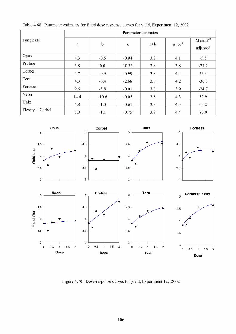
106
Table 4.68 Parameter estimates for fitted dose response curves for yield, Experiment 12, 2002
Parameter estimates
Fungicide a b k a+b a+bek
Mean R2
adjusted
Opus 4.3 -0.5 -0.94 3.8 4.1 -5.5 Proline 3.8 0.0 10.73 3.8 3.8 -27.2 Corbel 4.7 -0.9 -0.99 3.8 4.4 53.4 Tern 4.3 -0.4 -2.68 3.8 4.2 -30.5 Fortress 9.6 -5.8 -0.01 3.8 3.9 -24.7 Neon 14.4 -10.6 -0.05 3.8 4.3 57.9 Unix 4.8 -1.0 -0.61 3.8 4.3 63.2 Flexity + Corbel 5.0 -1.1 -0.75 3.8 4.4 80.0
Figure 4.70 Dose-response curves for yield, Experiment 12, 2002
Opus
3
3.5
4
4.5
5
Yiel
d t/h
a
Neon
3
3.5
4
4.5
5
0 0.5 1 1.5 2
Dose
Yiel
d t/h
a
Corbel
3
3.5
4
4.5
5Unix
3
3.5
4
4.5
5
Proline
3
3.5
4
4.5
5
0 0.5 1 1.5 2
Dose
Tern
3
3.5
4
4.5
5
0 0.5 1 1.5 2
Dose
Fortress
3
3.5
4
4.5
5
Corbel+Flexity
3
3.5
4
4.5
5
0 0.5 1 1.5 2
Dose

107
Table 4.69 Parameter estimates for fitted dose response curves for mildew control, experiment 25, 2004
Parameter estimates
Fungicide a b k a+b a+bek
Mean R2
adjusted
Opus 1.4 12.9 -0.33 14.3 10.7 63.7
Corbel 6.0 8.3 -0.89 14.3 9.4 93.4
Unix -2.2 16.5 -0.61 14.3 6.8 93.3
Fortress 8.4 5.9 -16.0 14.3 8.4 71.1
Neon 2.1 12.2 -1.78 14.3 4.2 71.3
Proline 2.3 12.0 -1.9 14.3 4.1 85.3
Tern 4.1 10.2 -3.2 14.3 4.5 74.8
Flexity 3.8 10.5 -2.6 14.3 4.6 72.4
Figure 4.71 Dose response curves for mildew control, experiment 25, 2004
Opus
0
5
10
15
20
25
% M
ildew
Neon
0
5
10
15
20
25
0 0.5 1 1.5 2
Dose
% M
ildew
Corbel
0
5
10
15
20
25Unix
0
5
10
15
20
25
Proline
0
5
10
15
20
25
0 0.5 1 1.5 2
Dose
Tern
0
5
10
15
20
25
0 0.5 1 1.5 2
Dose
Fortress
0
5
10
15
20
25
Flexity
0
5
10
15
20
25
0 0.5 1 1.5 2
Dose
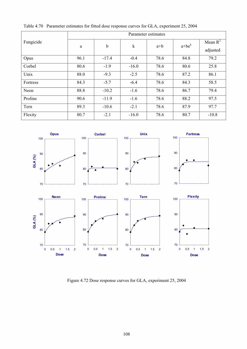
108
Table 4.70 Parameter estimates for fitted dose response curves for GLA, experiment 25, 2004
Parameter estimates
Fungicide a b k a+b a+bek
Mean R2
adjusted
Opus 96.1 -17.4 -0.4 78.6 84.8 79.2
Corbel 80.6 -1.9 -16.0 78.6 80.6 25.8
Unix 88.0 -9.3 -2.5 78.6 87.2 86.1
Fortress 84.3 -5.7 -6.4 78.6 84.3 58.5
Neon 88.8 -10.2 -1.6 78.6 86.7 79.4
Proline 90.6 -11.9 -1.6 78.6 88.2 97.5
Tern 89.3 -10.6 -2.1 78.6 87.9 97.7
Flexity 80.7 -2.1 -16.0 78.6 80.7 -10.8
Figure 4.72 Dose response curves for GLA, experiment 25, 2004
Opus
70
80
90
100
GLA
(%)
Neon
70
80
90
100
0 0.5 1 1.5 2
Dose
GLA
(%)
Corbel
70
80
90
100Unix
70
80
90
100
Proline
70
80
90
100
0 0.5 1 1.5 2
Dose
Tern
70
80
90
100
0 0.5 1 1.5 2
Dose
Fortress
70
80
90
100
Flexity
70
80
90
100
0 0.5 1 1.5 2
Dose

109
Table 4.71 Parameter estimates for fitted dose response curves for yield, experiment 25, 2004
Parameter estimates
Fungicide a b k a+b a+bek
Mean R2
adjusted
Opus 8.8 -3.1 -0.2 5.7 6.2 87.9
Corbel 6.4 -0.7 -1.1 5.7 6.2 49.7
Unix 5.5 0.2 -0.6 5.7 5.6 -32.6
Fortress 7.2 -1.5 -0.4 5.7 6.2 38.3
Neon 6.4 -0.7 -2.5 5.7 6.4 89.3
Proline 6.3 -0.6 -2.7 5.7 6.3 20.0
Tern 7.3 -1.6 -1.2 5.7 6.8 80.4
Flexity 6.6 -0.9 -1.8 5.7 6.5 20.3
Figure 4.73 Dose response curves for yield, experiment 25, 2004
Opus
5
6
7
8
Yie
ld t/
ha
Neon
5
6
7
8
0 0.5 1 1.5 2
Dose
Yiel
d t/h
a
Corbel
5
6
7
8Unix
5
6
7
8
Proline
5
6
7
8
0 0.5 1 1.5 2
Dose
Tern
5
6
7
8
0 0.5 1 1.5 2
Dose
Fortress
5
6
7
8
Flexity
5
6
7
8
0 0.5 1 1.5 2
Dose

110
Table 4.72 Parameter estimates for fitted dose response curves for specific weight, experiment 25, 2004
Parameter estimates
Fungicide a b k a+b a+bek
Mean R2
adjusted
Opus 71.0 -3.2 -0.3 67.8 68.7 50.8
Corbel 68.6 -0.7 -16.0 67.8 68.6 25.0
Unix 67.6 0.2 -0.3 67.8 67.8 -36.0
Fortress 70.7 -2.9 -0.7 67.8 69.2 80.9
Neon 69.6 -1.7 -1.2 67.8 69.0 78.1
Proline 69.6 -1.8 -1.2 67.8 69.1 83.9
Tern 70.4 -2.6 -2.1 67.8 70.1 88.5
Flexity 71.1 -3.2 -1.4 67.8 70.2 86.0
Figure 4.74 Dose response curves for specific weight, experiment 25, 2004
Opus
65
66
67
68
69
70
71
72
Sp
Wt.
Neon
65
66
67
68
69
70
71
72
0 0.5 1 1.5 2
Dose
Sp
Wt.
Corbel
65
66
67
68
69
70
71
72Unix
65
66
67
68
69
70
71
72
Proline
65
66
67
68
69
70
71
72
0 0.5 1 1.5 2
Dose
Tern
65
66
67
68
69
70
71
72
0 0.5 1 1.5 2
Dose
Fortress
65
66
67
68
69
70
71
72
Flexity
65
66
67
68
69
70
71
72
0 0.5 1 1.5 2
Dose
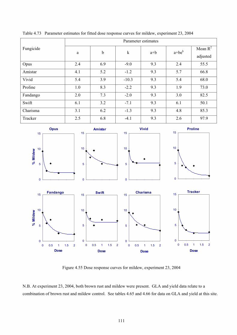
111
Table 4.73 Parameter estimates for fitted dose response curves for mildew, experiment 23, 2004
Parameter estimates
Fungicide a b k a+b a+bek
Mean R2
adjusted
Opus 2.4 6.9 -9.0 9.3 2.4 55.5
Amistar 4.1 5.2 -1.2 9.3 5.7 66.8
Vivid 5.4 3.9 -10.3 9.3 5.4 68.0
Proline 1.0 8.3 -2.2 9.3 1.9 73.0
Fandango 2.0 7.3 -2.0 9.3 3.0 82.5
Swift 6.1 3.2 -7.1 9.3 6.1 50.1
Charisma 3.1 6.2 -1.3 9.3 4.8 85.3
Tracker 2.5 6.8 -4.1 9.3 2.6 97.9
Figure 4.55 Dose response curves for mildew, experiment 23, 2004
N.B. At experiment 23, 2004, both brown rust and mildew were present. GLA and yield data relate to a
combination of brown rust and mildew control. See tables 4.65 and 4.66 for data on GLA and yield at this site.
Opus
0
5
10
15
% M
ildew
Fandango
0
5
10
15
0 0.5 1 1.5 2
Dose
% M
ildew
Amistar
0
5
10
15Vivid
0
5
10
15
Swift
0
5
10
15
0 0.5 1 1.5 2
Dose
Charisma
0
5
10
15
0 0.5 1 1.5 2
Dose
Proline
0
5
10
15
Tracker
0
5
10
15
0 0.5 1 1.5 2
Dose

112
5.0 CONCLUSIONS
• Robust, comparative dose-response data sets were gathered for the most widely used fungicides used on
wheat. This includes active ingredients from azole, morpholine, strobilurin, spiroketalamine,
benzamide and carboxanilide fungicide groups.
• Up to three years of data on fungicides launched in 2005 were gathered. These included boscalid (in
mixture with epoxiconazole in Tracker), dimoxystrobin (in mixture with epoxiconazole in Swing Gold),
fluoxastrobin (in mixture with prothioconazole in Fandango), metrafenone (Flexity) and
prothioconazole (Proline).
• The exponential function : y=a+be k dose described the range of dose-response variation across a wide
range of circumstances. The a, b and k parameters all have clear biological meaning.
• Fitted exponential curves describing the effect of fungicides on disease, green leaf area, yield and grain
quality typically explained a very high proportion (over 90%) of the variance in the data.
• The conclusions on individual treatments relate to single applications, applied under high disease
pressure, on a disease-susceptible variety. Where more resistant varieties are grown, disease pressure is
lower or the treatment forms part of a 2- or 3-spray programme, the appropriate dose will be lower.
This aspect of ‘Appropriate Dose’ is addressed in the new HGCA project No. 3026 Appropriate
Fungicide Dose sequences and mixtures in winter wheat according to disease risk
• Data on strobilurin performance against S. tritici clearly show a dramatic reduction in efficacy over the
period 2002 –2004. Despite measurements of the resistance allele (G143A) frequency indicating that
resistance levels were generally greater than 80% in 2004 there was still a measurable effect of
strobilurin fungicides against S. tritici.
• Analysis of data since 1994 indicate a significant reduction in activity of epoxiconazole (and by
inference, all other azole fungicides) against S. tritici. The observation of this effect in field trials has
been supported by laboratory-based data showing changes in the sensitivity of isolates of S. tritici.
• Information on these new products was published in the Wheat Disease Management Guide Update
2005 (published in February 2005) and on the HGCA web site as an interactive tool in March 2005.
113
• There were very substantial differences in dose-response curves between treatments. Significant
economic benefits would arise by using such data when selecting products and deciding on the dose to
apply.
Septoria tritici
• Opus (epoxiconazole) provided the most effective and consistent control of S. tritici.
• Tracker (a mixture of epoxiconazole and boscalid) gave equivalent control to epoxiconazole, despite
containing only 80% of the epoxiconazole dose in Opus.
• Proline (prothioconazole) gave control of S. tritici comparable to Opus.
• Fandango (prothioconazole plus fluoxastrobin) gave control of S. tritici comparable to Opus.
• Under high disease pressure, on a susceptible variety a three-quarter dose of Opus was needed for
consistent control.
• Compared with data from the mid 1990s there has been a clear loss of performance of the azoles against
S. tritici.
• The performance of strobilurins against S. tritici declined markedly during the period 2002-2004.
• Despite high levels of resistance to strobilurins in the S. tritici population at the start of 2004,
trifloxystrobin and pyraclostrobin both gave about 30% control of septoria in high disease pressure
situations.
Yellow rust
• The patterns of dose-response for yellow-rust control are substantially different from those for S. tritici.
The disease-control curves are very steep – i.e. the majority of the control of yellow rust is obtained
from the first quarter dose.
114
• Provided sprays are well timed, effective and consistent control of yellow rust can be obtained with
between a quarter and a half of the label-recommended dose.
• There is no evidence of any shift in activity of the triazoles against yellow rust since the mid 90s.
• The active ingredient prothioconazole (in Proline and Fandango) is slightly weak on yellow rust
compared with epoxiconazole. However, even in the very high disease-risk situations in these
experiments prothioconazole performed well.
• The strobilurins continue to be very effective against yellow rust. The addition of fluoxastrobin to
prothioconazole (in Fandango) eliminates the slight weakness of prothioconazole alone (as Proline).
Mildew
• There has been an almost complete loss of activity of the strobilurins against mildew during the course
of these experiments due to the development of resistance in the mildew population in the UK.
• There have been a number of new mildew fungicides introduced which has helped to compensate for
the loss of activity of the strobilurins. New active ingredients with specific activity against mildew
include metrafenone (Flexity), quinoxyfen (Fortress) and spiroxamine (Neon), all of which give good
control of the disease, particularly in when applied in a protectant situation.
Yield
• The full yield potential of disease-susceptible varieties such as Consort and Brigadier will not be
achieved in these experiments as only a single treatment is applied. Nevertheless, significant yield
responses were obtained in the experiments. Comparisons of full and untreated yields on Consort in
2004 showed a yield response of 1.1 t/ha for Opus, and 1.3 t/ha for Proline, Fandango and Tracker.
• The yield response to strobilurin treatment in these experiments is variable depending on the main
pathogens present and the resistance status of the S. tritici population. In 2001 and 2002 Vivid, on
average, gave yield responses 15-20% higher than Opus at S. tritici sites. In 2003 yield responses were
very similar but in 2004 Vivid treatment gave only 27% of the yield response of Opus treatment at
predominantly S. tritici sites.
• In brown rust experiments in 2002 yield responses to strobilurin treatment were often high because
additional control of S. tritici was obtained. This was not the case in 2004 when majority of the S. tritici
population was resistant to strobilurin fungicides.

115
• At septoria sites in 2004 yield responses to strobilurins were variable. At some sites no yield response
was obtained (Expt 24) but at others, (Expt 20) responses of 1.1 t/ha were achieved from a full dose of
Vivid. Some of this yield response is likely to be due to the control of other diseases such as brown rust
and S. nodorum but there was clearly significant control of S. tritici at some of these sites, despite very
high levels of resistance in the S. tritici population. The reasons for the variability in response to
strobilurin treatment at septoria sites are not fully understood although possible mechanisms are
discussed in a paper to be presented by W. S. Clark at the BCPC Conference – Crop Science &
Technology 2005 entitled “QoI resistance in Septoria tritici in the UK: implications for future use of
QoI fungicides”.
• In yellow rust experiments yield responses to low doses of fungicide were very large. In 2003 yield
responses to single applications at full label dose were on average 3.0 t/ha, with responses of 2.4 t/ha to
a quarter dose of Opus. In 2004 a yield response of 3.0t/ha was achieved from a single application of
one quarter of the label dose of Opus. A single full dose gave a yield response of over 3.5 t/ha. Vivid
and Swift gave yield responses of 1.5 t/ha to a quarter dose and 2.1 t/ha to a full dose. The recently
introduced products Fandango, Proline and Tracker all gave yield responses similar to Opus.
ACKNOWLEDGMENTS
These experiments were funded by the Home-Grown Cereals Authority. Thanks are due to the many
workers involved, including staff from ADAS, SAC and TAG who gathered the field data. Dr Anne
Ainsley, who carried out all of the statistical analysis, has our particular thanks.
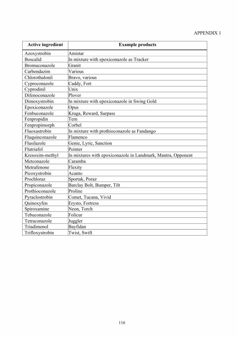
116
APPENDIX 1
Active ingredient Example products
Azoxystrobin Amistar Boscalid In mixture with epoxiconazole as Tracker Bromuconazole Granit Carbendazim Various Chlorothalonil Bravo, various Cyproconazole Caddy, Fort Cyprodinil Unix Difenoconazole Plover Dimoxystrobin In mixture with epoxiconazole in Swing Gold Epoxiconazole Opus Fenbuconazole Kruga, Reward, Surpass Fenpropidin Tern Fenpropimorph Corbel Fluoxastrobin In mixture with prothioconazole as Fandango Fluquinconazole Flamenco Flusilazole Genie, Lyric, Sanction Flutriafol Pointer Kresoxim-methyl In mixtures with epoxiconazole in Landmark, Mantra, Opponent Metconazole Caramba Metrafenone Flexity Picoxystrobin Acanto Prochloraz Sportak, Poraz Propiconazole Barclay Bolt, Bumper, Tilt Prothioconazole Proline Pyraclostrobin Comet, Tucana, Vivid Quinoxyfen Erysto, Fortress Spiroxamine Neon, Torch Tebuconazole Folicur Tetraconazole Juggler Triadimenol Bayfidan Trifloxystrobin Twist, Swift

117
APPENDIX 2
Products Active ingredient
Acanto Picoxystrobin Amistar Azoxystrobin Bayfidan Triadimenol Bravo Chlorothalonil Bumper Propiconazole Caddy Cyproconazole Caramba Metconazole Comet Pyraclostrobin Corbel Fenpropimorph Erysto Quinoxyfen Fandango Fluoxastrobin + prothioconazole Flamenco Fluquinconazole Flexity Metrafenone Folicur Tebuconazole Fort Cyproconazole Fortress Quinoxyfen Genie Flusilazole Granit Bromuconazole Juggler Tetraconazole Kruga Fenbuconazole Landmark Kresoxim-methyl + epoxiconazole Lyric Flusilazole Mantra Kresoxim-methyl + epoxiconazole + fenpropimorph Neon Spiroxamine Opponent Kresoxim-methyl + epoxiconazole + pyraclostrobin Opus Epoxiconazole Plover Difenoconazole Pointer Flutriafol Poraz Prochloraz Proline Prothioconazole Reward Fenbuconazole Sanction Flusilazole Sportak Prochloraz Surpass Fenbuconazole Swift Trifloxystrobin Swing Gold Dimoxystrobin + epoxiconazole Tern Fenpropidin Tilt Propiconazole Torch Spiroxamine Tracker Boscalid + epoxiconazole Tucana Pyraclostrobin Twist Trifloxystrobin Unix Cyprodinil Vivid Pyraclostrobin