FUNDAMENTALS OF THERMAL-FLUID SCIENCES...

22–1 THE VIEW FACTORRadiation heat transfer between surfaces depends on the orientation of thesurfaces relative to each other as well as their radiation properties and tem-peratures, as illustrated in Fig. 22–1. For example, a camper will make themost use of a campfire on a cold night by standing as close to the fire as pos-sible and by blocking as much of the radiation coming from the fire by turn-ing her front to the fire instead of her side. Likewise, a person will maximizethe amount of solar radiation incident on him and take a sunbath by lyingdown on his back instead of standing up on his feet.

To account for the effects of orientation on radiation heat transfer betweentwo surfaces, we define a new parameter called the view factor, which is apurely geometric quantity and is independent of the surface properties andtemperature. It is also called the shape factor, configuration factor, and anglefactor. The view factor based on the assumption that the surfaces are diffuseemitters and diffuse reflectors is called the diffuse view factor, and the viewfactor based on the assumption that the surfaces are diffuse emitters but spec-ular reflectors is called the specular view factor. In this book, we will considerradiation exchange between diffuse surfaces only, and thus the term view fac-tor will simply mean diffuse view factor.

The view factor from a surface i to a surface j is denoted by Fi → j or just Fij,and is defined as

Fij � the fraction of the radiation leaving surface i that strikes surface j directly

The notation Fi → j is instructive for beginners, since it emphasizes that theview factor is for radiation that travels from surface i to surface j. However,this notation becomes rather awkward when it has to be used many times in aproblem. In such cases, it is convenient to replace it by its shorthand ver-sion Fij.

Therefore, the view factor F12 represents the fraction of radiation leavingsurface 1 that strikes surface 2 directly, and F21 represents the fraction of theradiation leaving surface 2 that strikes surface 1 directly. Note that the radia-tion that strikes a surface does not need to be absorbed by that surface. Also,radiation that strikes a surface after being reflected by other surfaces is notconsidered in the evaluation of view factors.

To develop a general expression for the view factor, consider two differen-tial surfaces dA1 and dA2 on two arbitrarily oriented surfaces A1 and A2, re-spectively, as shown in Fig. 22–2. The distance between dA1 and dA2 is r, andthe angles between the normals of the surfaces and the line that connects dA1

and dA2 are u1 and u2, respectively. Surface 1 emits and reflects radiation dif-fusely in all directions with a constant intensity of I1, and the solid angle sub-tended by dA2 when viewed by dA1 is dv21.

The rate at which radiation leaves dA1 in the direction of u1 is I1 cos u1dA1.Noting that dv21 � dA2 cos u2 /r 2, the portion of this radiation that strikesdA2 is

d → d � I1 cos u1 dA1 dv21 � I1 cos u1 dA1 (22–1)dA2 cos u2

r 2A2A1

�Q

■

986FUNDAMENTALS OF THERMAL-FLUID SCIENCES

Pointsource

Surface 3

Surface 1Surface 2

FIGURE 22–1Radiation heat exchange betweensurfaces depends on the orientationof the surfaces relative to each other,and this dependence on orientation isaccounted for by the view factor.

dA1

d 21�

dA2

A1

A21θ

2θn2

n1

r

FIGURE 22–2Geometry for the determination of theview factor between two surfaces.

cen54261_ch22.qxd 1/25/04 3:00 PM Page 986

The total rate at which radiation leaves dA1 (via emission and reflection) in alldirections is the radiosity (which is J1 � pI1) times the surface area,

d � J1 dA1 � pI1 dA1 (22–2)

Then the differential view factor dFd → d , which is the fraction of radiationleaving dA1 that strikes dA2 directly, becomes

dFd → d � � dA2 (22–3)

The differential view factor dFd → d can be determined from Eq. 22–3 byinterchanging the subscripts 1 and 2.

The view factor from a differential area dA1 to a finite area A2 can bedetermined from the fact that the fraction of radiation leaving dA1 that strikesA2 is the sum of the fractions of radiation striking the differential areas dA2.Therefore, the view factor Fd → is determined by integrating dFd → dover A2,

Fd → � dA2 (22–4)

The total rate at which radiation leaves the entire A1 (via emission and re-flection) in all directions is

� J1A1 � pI1A1 (22–5)

The portion of this radiation that strikes dA2 is determined by considering theradiation that leaves dA1 and strikes dA2 (given by Eq. 22–1), and integratingit over A1,

→ d � d → d � dA1 (22–6)

Integration of this relation over A2 gives the radiation that strikes the entire A2,

→ � → d � dA1 dA2 (22–7)

Dividing this by the total radiation leaving A1 (from Eq. 22–5) gives the frac-tion of radiation leaving A1 that strikes A2, which is the view factor F → (orF12 for short),

F12 � F → � � dA1 dA2 (22–8)

The view factor F → is readily determined from Eq. 22–8 by interchangingthe subscripts 1 and 2,

F21 � F → � � dA1 dA2 (22–9)�A2 �A1

cos u1 cos u2

pr 21A2

Q·A2 → A1

Q·A2

A1A2

A1A2

�A2 �A1

cos u1 cos u2

pr 21A1

Q·A1 → A2

Q·A1

A2A1

A2A1

�A2 �A1

I1 cos u1 cos u2

r 2A2A1

�Q�

A2

A2A1

�Q

�A1

I1 cos u1 cos u2 dA2

r 2A2A1

�Q�

A1

A2A1

�Q

A1

�Q

�A2

cos u1 cos u2

pr 2A2A1

A2A1A2A1

A1A2

cos u1 cos u2

pr 2

Q·dA1 → dA2

Q·dA1

A2A1

A2A1

A1

�Q

CHAPTER 22987

cen54261_ch22.qxd 1/25/04 3:00 PM Page 987

Note that I1 is constant but r, u1, and u2 are variables. Also, integrations can beperformed in any order since the integration limits are constants. These rela-tions confirm that the view factor between two surfaces depends on their rel-ative orientation and the distance between them.

Combining Eqs. 22–8 and 22–9 after multiplying the former by A1 and thelatter by A2 gives

A1F12 � A2F21 (22–10)

which is known as the reciprocity relation for view factors. It allows the cal-culation of a view factor from a knowledge of the other.

The view factor relations developed above are applicable to any two sur-faces i and j provided that the surfaces are diffuse emitters and diffuse reflec-tors (so that the assumption of constant intensity is valid). For the special caseof j � i, we have

Fi → i � the fraction of radiation leaving surface i that strikes itself directly

Noting that in the absence of strong electromagnetic fields radiation beamstravel in straight paths, the view factor from a surface to itself will be zero un-less the surface “sees” itself. Therefore, Fi → i � 0 for plane or convex surfacesand Fi → i � 0 for concave surfaces, as illustrated in Fig. 22–3.

The value of the view factor ranges between zero and one. The limiting caseFi → j � 0 indicates that the two surfaces do not have a direct view of eachother, and thus radiation leaving surface i cannot strike surface j directly. Theother limiting case Fi → j � 1 indicates that surface j completely surrounds sur-face i, so that the entire radiation leaving surface i is intercepted by surface j.For example, in a geometry consisting of two concentric spheres, the entireradiation leaving the surface of the smaller sphere (surface 1) will strike thelarger sphere (surface 2), and thus F1 → 2 � 1, as illustrated in Fig. 22–4.

The view factor has proven to be very useful in radiation analysis because itallows us to express the fraction of radiation leaving a surface that strikes an-other surface in terms of the orientation of these two surfaces relative to eachother. The underlying assumption in this process is that the radiation a surfacereceives from a source is directly proportional to the angle the surface sub-tends when viewed from the source. This would be the case only if theradiation coming off the source is uniform in all directions throughout itssurface and the medium between the surfaces does not absorb, emit, or scatterradiation. That is, it will be the case when the surfaces are isothermal anddiffuse emitters and reflectors and the surfaces are separated by a non-participating medium such as a vacuum or air.

The view factor F1 → 2 between two surfaces A1 and A2 can be determined ina systematic manner first by expressing the view factor between two differen-tial areas dA1 and dA2 in terms of the spatial variables and then by performingthe necessary integrations. However, this approach is not practical, since, evenfor simple geometries, the resulting integrations are usually very complex anddifficult to perform.

View factors for hundreds of common geometries are evaluated and the re-sults are given in analytical, graphical, and tabular form in several publica-tions. View factors for selected geometries are given in Tables 22–1 and 22–2in analytical form and in Figs. 22–5 to 22–8 in graphical form. The view


F1 → 1 = 01

2

3

F2 → 2 = 0

F3 → 3 ≠ 0

(a) Plane surface

(b) Convex surface

(c) Concave surface

FIGURE 22–3The view factor from a surfaceto itself is zero for plane orconvex surfaces and nonzerofor concave surfaces.

Outersphere

2

F1 → 2 = 1

Innersphere

1

FIGURE 22–4In a geometry that consists of twoconcentric spheres, the view factorF1 → 2 � 1 since the entire radiationleaving the surface of the smallersphere will be intercepted by thelarger sphere.

cen54261_ch22.qxd 1/25/04 3:00 PM Page 988

factors in Table 22–1 are for three-dimensional geometries. The view factorsin Table 22–2, on the other hand, are for geometries that are infinitely longin the direction perpendicular to the plane of the paper and are thereforetwo-dimensional.

22–2 VIEW FACTOR RELATIONSRadiation analysis on an enclosure consisting of N surfaces requires the eval-uation of N2 view factors, and this evaluation process is probably the mosttime-consuming part of a radiation analysis. However, it is neither practicalnor necessary to evaluate all of the view factors directly. Once a sufficientnumber of view factors are available, the rest of them can be determined byutilizing some fundamental relations for view factors, as discussed next.

■

CHAPTER 22989

TABLE 22–1

View factor expressions for some common geometries of finite size (3D)

L

YX

i

j

j

i

rj

ri L

Z

Y Xi

j

2——πXY

(1 + X2)(1 + Y 2)———————1 + X2 + Y 2

X = X/L and Y = Y/LAligned parallel rectangles

Geometry Relation––

Fi → j =

Fi → j = S – ( )

ln–––– –––– ––

––

––

X———–—(1 + Y 2)1/2

+ X(1 + Y 2)1/2 tan–1––––––

––

Y———–—(1 + X2)1/2

+ Y(1 + X2)1/2 tan–1––––

– X tan–1 X – Y tan–1 Y–– –– ––––

––––

1—–πW

1—W

1—H

H = Z /X and W = Y/XPerpendicular rectangleswith a common edge

Fi → j = W tan–1 + H tan–1

1———–——(H2 + W2)1/2

– (H2 + W2)1/2 tan–1

(1 + W2)(1 + H2)———————1 + W2 + H2

1–4

+ ln

1 + Rj2

——–Ri

2

rj—ri

Ri = ri /L and Rj = rj /LCoaxial parallel disks

S = 1 +

S2 – 4

(

)

2 1/2

W2W2(1 + W2 + H2)————————

(1 + W2)(W2 + H2)×

H2H2(1 + H2 + W2)————————

(1 + H2)(H2 + W2)×

1–2

1/2

cen54261_ch22.qxd 1/25/04 3:00 PM Page 989

1 The Reciprocity RelationThe view factors Fi → j and Fj → i are not equal to each other unless the areas ofthe two surfaces are. That is,

Fj → i � Fi → j when Ai � Aj

Fj → i � Fi → j when Ai � Aj


TABLE 22–2

View factor expressions for some infinitely long (2D) geometries

Parallel plates with midlinesconnected by perpendicular line

Geometry Relation

Fi → j = 1 – sin α

Perpendicular plates with a common edge

Three-sided enclosure

Infinite plane and row of cylinders

Inclined plates of equal widthand with a common edge

1–2

Fi → j =

Wi = wi /L and Wj = wj /L

[(Wi + Wj)2 + 4]1/2 – (Wj – Wi)

2 + 4]1/2

———————————————2Wi

Fi → j =wi + wj – wk—————

2wi

j

iwi

wj

L

i

j

wi

j

iα

w

w

k j

i

i

jD

wj

wj

wi

wk

s

Fi → j = ( )wj—wi

1 +wj—wi

1 + –2 1/21–

2

Fi → j = 1 – 1 – ( )( )

D—s

D—s

+ tan–1

2 1/2

1/2s2 – D2———

D2

cen54261_ch22.qxd 1/25/04 3:00 PM Page 990

CHAPTER 22991

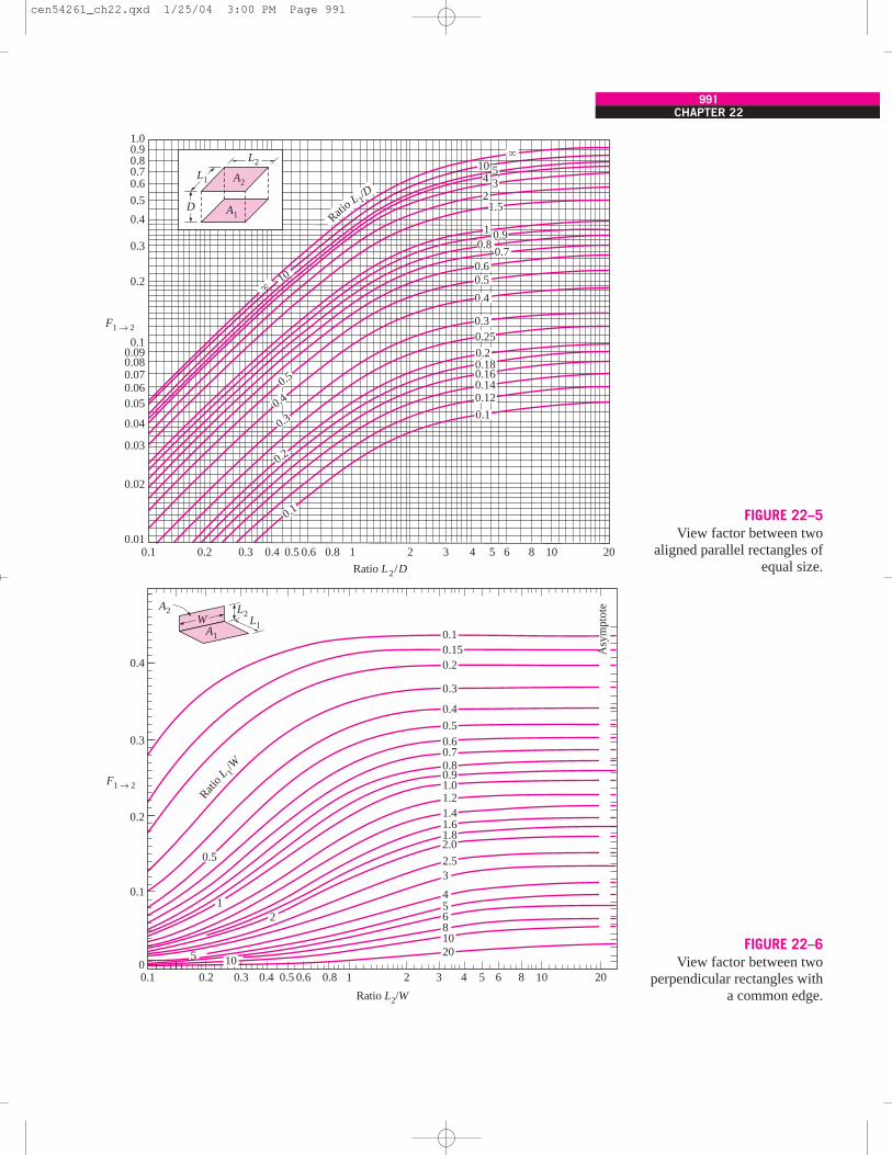
FIGURE 22–5View factor between two

aligned parallel rectangles ofequal size.

10

0.9

1.5

0.80.7

0.60.5

0.4

0.30.25

0.2

0.1

0.1

0.2

0.30.4

0.5

10�

�

0.140.16

0.12

53

1

A2

A1

L2

L1

Ratio L 1

/D

Ratio L2/D

0.1 0.2 0.3 0.4 0.5 0.6 0.8 1 2 3 4 5 6 8 10 20

1.00.90.80.70.6

0.5

0.4

0.3

0.2

0.1

0.01

0.02

0.03

0.04

0.050.060.070.080.09

4

2

0.18

F1 → 2

DRati

o L 1/W

0.150.1

0.2

0.3

0.4

0.50.60.70.8

1.01.21.41.6

2.50.5

2

Ratio L2/W

0.20.1 0.3 0.4 0.5 0.6 0.8 1 2 3 4 5 6 8 10 20

145

810

5

0.9

1.82.0

20

6

3

A2

A1

L2L1

W

0.4

0.3

0.2

0.1

0

Asy

mpt

ote

10

F1 → 2

FIGURE 22–6View factor between two

perpendicular rectangles witha common edge.

cen54261_ch22.qxd 1/25/04 3:00 PM Page 991


FIGURE 22–7View factor between twocoaxial parallel disks.

54

3

2 1.5

1.25

1.0

0.8

0.60.50.4

r2 /L = 0.3

r2 /L = 8

6

r2

r1

L /r1

2

1

1.0

0.9

0.8

0.7

0.6

0.5

0.4

0.3

0.2

0.1

00.1 0.2 0.3 0.4 0.6 1.0 2 3 4 5 6 8 10

F1 → 2

L

FIGURE 22–8View factors for two concentric cylinders of finite length: (a) outer cylinder to inner cylinder; (b) outer cylinder to itself.

r1/r2

L/r2 = �

L/r 2 =

�

4

2

1

1.0

0.9

0.8

0.7

0.6

0.5

0.4

0.3

0.2

0.1

0

0.5

0.25

0.25

0 0.2 0.4 0.6 0.8 1.00.1 0.3 0.5 0.7 0.9

r1/r2

0 0.2 0.4 0.6 0.8 1.0

0.5

0.1

12

1.0

0.8

0.6

0.4

0.2

A1

L

r1

r2

A2

F2 → 1

F2 → 2

cen54261_ch22.qxd 1/25/04 3:00 PM Page 992

We have shown earlier the pair of view factors Fi → j and Fj → i are related toeach other by

AiFi → j � AjFj → i (22–11)

This relation is referred to as the reciprocity relation or the reciprocity rule,and it enables us to determine the counterpart of a view factor from a knowl-edge of the view factor itself and the areas of the two surfaces. When deter-mining the pair of view factors Fi → j and Fj → i, it makes sense to evaluate firstthe easier one directly and then the more difficult one by applying the reci-procity relation.

2 The Summation RuleThe radiation analysis of a surface normally requires the consideration of theradiation coming in or going out in all directions. Therefore, most radiationproblems encountered in practice involve enclosed spaces. When formulatinga radiation problem, we usually form an enclosure consisting of the surfacesinteracting radiatively. Even openings are treated as imaginary surfaces withradiation properties equivalent to those of the opening.

The conservation of energy principle requires that the entire radiation leav-ing any surface i of an enclosure be intercepted by the surfaces of the enclosure. Therefore, the sum of the view factors from surface i of an en-closure to all surfaces of the enclosure, including to itself, must equal unity.This is known as the summation rule for an enclosure and is expressed as(Fig. 22–9)

Fi → j � 1 (22–12)

where N is the number of surfaces of the enclosure. For example, applying thesummation rule to surface 1 of a three-surface enclosure yields

F1 → j � F1 → 1 � F1 → 2 � F1 → 3 � 1

The summation rule can be applied to each surface of an enclosure by vary-ing i from 1 to N. Therefore, the summation rule applied to each of the N sur-faces of an enclosure gives N relations for the determination of the viewfactors. Also, the reciprocity rule gives N(N � 1) additional relations. Thenthe total number of view factors that need to be evaluated directly for anN-surface enclosure becomes

N2 � [N � N(N � 1)] � N(N � 1)

For example, for a six-surface enclosure, we need to determine only � 6(6 � 1) � 15 of the 62 � 36 view factors directly. The remaining

21 view factors can be determined from the 21 equations that are obtained byapplying the reciprocity and the summation rules.

12

12

12

12

�3

j�1

�N

j�1

CHAPTER 22993

Surface i

FIGURE 22–9Radiation leaving any surface i ofan enclosure must be interceptedcompletely by the surfaces of theenclosure. Therefore, the sum of

the view factors from surface i toeach one of the surfaces of the

enclosure must be unity.

cen54261_ch22.qxd 1/25/04 3:00 PM Page 993


EXAMPLE 22–1 View Factors Associated with Two ConcentricSpheres

Determine the view factors associated with an enclosure formed by two spheres,shown in Fig. 22–10.

SOLUTION The view factors associated with two concentric spheres are to bedetermined.Assumptions The surfaces are diffuse emitters and reflectors.Analysis The outer surface of the smaller sphere (surface 1) and inner surfaceof the larger sphere (surface 2) form a two-surface enclosure. Therefore, N � 2and this enclosure involves N 2 � 22 � 4 view factors, which are F11, F12, F21,and F22. In this two-surface enclosure, we need to determine only

N(N � 1) � � 2(2 � 1) � 1

view factor directly. The remaining three view factors can be determined by theapplication of the summation and reciprocity rules. But it turns out that we candetermine not only one but two view factors directly in this case by a simpleinspection:

F11 � 0, since no radiation leaving surface 1 strikes itself

F12 � 1, since all radiation leaving surface 1 strikes surface 2

Actually it would be sufficient to determine only one of these view factors byinspection, since we could always determine the other one from the summationrule applied to surface 1 as F11 � F12 � 1.

The view factor F21 is determined by applying the reciprocity relation to sur-faces 1 and 2:

A1F12 � A2F21

which yields

F21 � F12 � � 1 �

Finally, the view factor F22 is determined by applying the summation rule to sur-face 2:

F21 � F22 � 1

and thus

F22 � 1 � F21 � 1 �

Discussion Note that when the outer sphere is much larger than the innersphere (r2 r1), F22 approaches one. This is expected, since the fraction ofradiation leaving the outer sphere that is intercepted by the inner sphere will benegligible in that case. Also note that the two spheres considered above do notneed to be concentric. However, the radiation analysis will be most accurate forthe case of concentric spheres, since the radiation is most likely to be uniformon the surfaces in that case.

�r1

r2�2

�r1

r2�24pr 2

1

4pr 22

A1

A2

12

12

r1r2

21

FIGURE 22–10The geometry consideredin Example 22–1.

cen54261_ch22.qxd 1/25/04 3:00 PM 94

3 The Superposition RuleSometimes the view factor associated with a given geometry is not availablein standard tables and charts. In such cases, it is desirable to express the givengeometry as the sum or difference of some geometries with known view fac-tors, and then to apply the superposition rule, which can be expressed as theview factor from a surface i to a surface j is equal to the sum of the view fac-tors from surface i to the parts of surface j. Note that the reverse of this is nottrue. That is, the view factor from a surface j to a surface i is not equal to thesum of the view factors from the parts of surface j to surface i.

Consider the geometry in Fig. 22–11, which is infinitely long in thedirection perpendicular to the plane of the paper. The radiation that leavessurface 1 and strikes the combined surfaces 2 and 3 is equal to the sum of theradiation that strikes surfaces 2 and 3. Therefore, the view factor from surface1 to the combined surfaces of 2 and 3 is

F1 → (2, 3) � F1 → 2 � F1 → 3 (22–13)

Suppose we need to find the view factor F1 → 3. A quick check of the view fac-tor expressions and charts in this section will reveal that such a view factorcannot be evaluated directly. However, the view factor F1 → 3 can be deter-mined from Eq. 22–13 after determining both F1 → 2 and F1 → (2, 3) from thechart in Table 22–2. Therefore, it may be possible to determine some difficultview factors with relative ease by expressing one or both of the areas as thesum or differences of areas and then applying the superposition rule.

To obtain a relation for the view factor F(2, 3) → 1, we multiply Eq. 22–13 by A1,

A1F1 → (2, 3) � A1F1 → 2 � A1F1 → 3

and apply the reciprocity relation to each term to get

(A2 � A3)F(2, 3) → 1 � A2F2 → 1 � A3F3 → 1

or

F(2, 3) → 1 � (22–14)

Areas that are expressed as the sum of more than two parts can be handled ina similar manner.

A2 F2 → 1 � A3 F3 → 1

A2 � A3

CHAPTER 22995

= +

1

2

1

2

3

1

3

F1 → (2, 3) = F1 → 2 + F1 → 3

FIGURE 22–11The view factor from a surface to a

composite surface is equal to the sumof the view factors from the surface to

the parts of the composite surface.

r1 = 10 cm1

2

r3 = 8 cm

r2 = 5 cm3

FIGURE 22–12The cylindrical enclosure

considered in Example 22–2.

EXAMPLE 22–2 Fraction of Radiation Leavingthrough an Opening

Determine the fraction of the radiation leaving the base of the cylindrical en-closure shown in Fig. 22–12 that escapes through a coaxial ring opening at itstop surface. The radius and the length of the enclosure are r1 � 10 cm andL � 10 cm, while the inner and outer radii of the ring are r2 � 5 cm andr3 � 8 cm, respectively.

cen54261_ch22.qxd 1/25/04 3:00 PM Page 995

4 The Symmetry RuleThe determination of the view factors in a problem can be simplified furtherif the geometry involved possesses some sort of symmetry. Therefore, it isgood practice to check for the presence of any symmetry in a problem beforeattempting to determine the view factors directly. The presence of symmetrycan be determined by inspection, keeping the definition of the view factor inmind. Identical surfaces that are oriented in an identical manner with respectto another surface will intercept identical amounts of radiation leaving thatsurface. Therefore, the symmetry rule can be expressed as two (or more) sur-faces that possess symmetry about a third surface will have identical view fac-tors from that surface (Fig. 22–13).

The symmetry rule can also be expressed as if the surfaces j and k are sym-metric about the surface i then Fi → j � Fi → k. Using the reciprocity rule, wecan show that the relation Fj → i � Fk → i is also true in this case.


SOLUTION The fraction of radiation leaving the base of a cylindrical enclosurethrough a coaxial ring opening at its top surface is to be determined.Assumptions The base surface is a diffuse emitter and reflector.Analysis We are asked to determine the fraction of the radiation leaving thebase of the enclosure that escapes through an opening at the top surface.Actually, what we are asked to determine is simply the view factor F1 → ring fromthe base of the enclosure to the ring-shaped surface at the top.

We do not have an analytical expression or chart for view factors between acircular area and a coaxial ring, and so we cannot determine F1 → ring directly.However, we do have a chart for view factors between two coaxial parallel disks,and we can always express a ring in terms of disks.

Let the base surface of radius r1 � 10 cm be surface 1, the circular area ofr2 � 5 cm at the top be surface 2, and the circular area of r3 � 8 cm be sur-face 3. Using the superposition rule, the view factor from surface 1 to surface 3can be expressed as

F1 → 3 � F1 → 2 � F1 → ring

since surface 3 is the sum of surface 2 and the ring area. The view factors F1 → 2

and F1 → 3 are determined from the chart in Fig. 22–7.

� 1 and � 0.5 → F1 → 2 � 0.11(Fig. 22–7)

� 1 and � 0.8 → F1 → 3 � 0.28(Fig. 22–7)

Therefore,

F1 → ring � F1 → 3 � F1 → 2 � 0.28 � 0.11 � 0.17

which is the desired result. Note that F1 → 2 and F1 → 3 represent the fractions ofradiation leaving the base that strike the circular surfaces 2 and 3, respectively,and their difference gives the fraction that strikes the ring area.

r3

L�

8 cm10 cm

Lr1

�10 cm10 cm

r2

L�

5 cm10 cm

Lr1

�10 cm10 cm

1

23

F1 → 2 = F1 → 3

F2 → 1 = F3 → 1 ) (Also,

FIGURE 22–13Two surfaces that are symmetric abouta third surface will have the sameview factor from the third surface.

cen54261_ch22.qxd 1/25/04 3:00 PM Page 996

CHAPTER 22997

EXAMPLE 22–3 View Factors Associated with a Tetragon

Determine the view factors from the base of the pyramid shown in Fig. 22–14to each of its four side surfaces. The base of the pyramid is a square, and itsside surfaces are isosceles triangles.

SOLUTION The view factors from the base of a pyramid to each of its four sidesurfaces for the case of a square base are to be determined.Assumptions The surfaces are diffuse emitters and reflectors.Analysis The base of the pyramid (surface 1) and its four side surfaces (sur-faces 2, 3, 4, and 5) form a five-surface enclosure. The first thing we noticeabout this enclosure is its symmetry. The four side surfaces are symmetricabout the base surface. Then, from the symmetry rule, we have

F12 � F13 � F14 � F15

Also, the summation rule applied to surface 1 yields

F1j � F11 � F12 � F13 � F14 � F15 � 1

However, F11 � 0, since the base is a flat surface. Then the two relationsabove yield

F12 � F13 � F14 � F15 � 0.25

Discussion Note that each of the four side surfaces of the pyramid receiveone-fourth of the entire radiation leaving the base surface, as expected. Alsonote that the presence of symmetry greatly simplified the determination of theview factors.

�5

j �1

1

4

5

3

2

FIGURE 22–14The pyramid considered

in Example 22–3.

EXAMPLE 22–4 View Factors Associated with a Triangular Duct

Determine the view factor from any one side to any other side of the infinitelylong triangular duct whose cross section is given in Fig. 22–15.

SOLUTION The view factors associated with an infinitely long triangular ductare to be determined.Assumptions The surfaces are diffuse emitters and reflectors.Analysis The widths of the sides of the triangular cross section of the duct areL1, L2, and L3, and the surface areas corresponding to them are A1, A2, and A3,respectively. Since the duct is infinitely long, the fraction of radiation leavingany surface that escapes through the ends of the duct is negligible. Therefore,the infinitely long duct can be considered to be a three-surface enclosure,N � 3.

This enclosure involves N 2 � 32 � 9 view factors, and we need to determine

N(N � 1) � � 3(3 � 1) � 312

12

1

23L3 L2

L1

FIGURE 22–15The infinitely long triangular duct


cen54261_ch22.qxd 1/25/04 3:00 PM Page 997

View Factors between Infinitely Long Surfaces:The Crossed-Strings MethodMany problems encountered in practice involve geometries of constant crosssection such as channels and ducts that are very long in one direction relative


of these view factors directly. Fortunately, we can determine all three of them byinspection to be

F11 � F22 � F33 � 0

since all three surfaces are flat. The remaining six view factors can be deter-mined by the application of the summation and reciprocity rules.

Applying the summation rule to each of the three surfaces gives

F11 � F12 � F13 � 1

F21 � F22 � F23 � 1

F31 � F32 � F33 � 1

Noting that F11 � F22 � F33 � 0 and multiplying the first equation by A1, thesecond by A2, and the third by A3 gives

A1F12 � A1F13 � A1

A2F21 � A2F23 � A2

A3F31 � A3F32 � A3

Finally, applying the three reciprocity relations A1F12 � A2F21, A1F13 � A3F31,and A2F23 � A3F32 gives

A1F12 � A1F13 � A1

A1F12 � A2F23 � A2

A1F13 � A2F23 � A3

This is a set of three algebraic equations with three unknowns, which can besolved to obtain

F12 � �

F13 � �

F23 � � (22–15)

Discussion Note that we have replaced the areas of the side surfaces by theircorresponding widths for simplicity, since A � Ls and the length s can be fac-tored out and canceled. We can generalize this result as the view factor from asurface of a very long triangular duct to another surface is equal to the sum ofthe widths of these two surfaces minus the width of the third surface, dividedby twice the width of the first surface.

L2 � L3 � L1

2L2

A2 � A3 � A1

2A2

L1 � L3 � L2

2L1

A1 � A3 � A2

2A1

L1 � L2 � L3

2L1

A1 � A2 � A3

2A1

cen54261_ch22.qxd 1/25/04 3:00 PM Page 998

to the other directions. Such geometries can conveniently be considered to betwo-dimensional, since any radiation interaction through their end surfaceswill be negligible. These geometries can subsequently be modeled as beinginfinitely long, and the view factor between their surfaces can be determinedby the amazingly simple crossed-strings method developed by H. C. Hottel inthe 1950s. The surfaces of the geometry do not need to be flat; they can beconvex, concave, or any irregular shape.

To demonstrate this method, consider the geometry shown in Fig. 22–16,and let us try to find the view factor F1 → 2 between surfaces 1 and 2. The firstthing we do is identify the endpoints of the surfaces (the points A, B, C, and D)and connect them to each other with tightly stretched strings, which areindicated by dashed lines. Hottel has shown that the view factor F1 → 2 can beexpressed in terms of the lengths of these stretched strings, which are straightlines, as

F1 → 2 � (22–16)

Note that L5 � L6 is the sum of the lengths of the crossed strings, and L3 � L4

is the sum of the lengths of the uncrossed strings attached to the endpoints.Therefore, Hottel’s crossed-strings method can be expressed verbally as

Fi → j � (22–17)

The crossed-strings method is applicable even when the two surfaces consid-ered share a common edge, as in a triangle. In such cases, the common edgecan be treated as an imaginary string of zero length. The method can also beapplied to surfaces that are partially blocked by other surfaces by allowing thestrings to bend around the blocking surfaces.

� (Crossed strings) � � (Uncrossed strings)2 � (String on surface i)

(L5 � L6) � (L3 � L4)2L1

CHAPTER 22999

L2

L1

L5

L3

AB

DC

L4

L6

1

2

FIGURE 22–16Determination of the view factor

F1 → 2 by the application ofthe crossed-strings method.

EXAMPLE 22–5 The Crossed-Strings Method for View Factors

Two infinitely long parallel plates of widths a � 12 cm and b � 5 cm are lo-cated a distance c � 6 cm apart, as shown in Fig. 22–17. (a) Determine theview factor F1 → 2 from surface 1 to surface 2 by using the crossed-stringsmethod. (b) Derive the crossed-strings formula by forming triangles on the givengeometry and using Eq. 22–15 for view factors between the sides of triangles.

SOLUTION The view factors between two infinitely long parallel plates are tobe determined using the crossed-strings method, and the formula for the viewfactor is to be derived.Assumptions The surfaces are diffuse emitters and reflectors.Analysis (a) First we label the endpoints of both surfaces and draw straightdashed lines between the endpoints, as shown in Fig. 22–17. Then we identifythe crossed and uncrossed strings and apply the crossed-strings method(Eq. 22–17) to determine the view factor F1 → 2:

F1 → 2 �� (Crossed strings) � � (Uncrossed strings)

2 � (String on surface 1)�

(L5 � L6) � (L3 � L4)2L1

C D

b = L2 = 5 cm

c = 6 cm

a = L1 = 12 cm

A B

L3

L5L6

L4

1

2

FIGURE 22–17The two infinitely long parallel

plates considered in Example 22–5.

cen54261_ch22.qxd 1/25/04 3:00 PM Page 999

22–3 RADIATION HEAT TRANSFER:BLACK SURFACES

So far, we have considered the nature of radiation, the radiation properties ofmaterials, and the view factors, and we are now in a position to consider therate of heat transfer between surfaces by radiation. The analysis of radiationexchange between surfaces, in general, is complicated because of reflection: aradiation beam leaving a surface may be reflected several times, with partialreflection occurring at each surface, before it is completely absorbed. Theanalysis is simplified greatly when the surfaces involved can be approximated

■


where

L1 � a � 12 cm L4 � � 9.22 cm

L2 � b � 5 cm L5 � � 7.81 cm

L3 � c � 6 cm L6 � � 13.42 cm

Substituting,

F1 → 2 � � 0.250

(b) The geometry is infinitely long in the direction perpendicular to the plane ofthe paper, and thus the two plates (surfaces 1 and 2) and the two openings(imaginary surfaces 3 and 4) form a four-surface enclosure. Then applying thesummation rule to surface 1 yields

F11 � F12 � F13 � F14 � 1

But F11 � 0 since it is a flat surface. Therefore,

F12 � 1 � F13 � F14

where the view factors F13 and F14 can be determined by considering the trian-gles ABC and ABD, respectively, and applying Eq. 22–15 for view factors be-tween the sides of triangles. We obtain

F13 � , F14 �

Substituting,

F12 � 1 �

�

which is the desired result. This is also a miniproof of the crossed-stringsmethod for the case of two infinitely long plain parallel surfaces.

(L5 � L6) � (L3 � L4)2L1

L1 � L3 � L6

2L1�

L1 � L4 � L5

2L1

L1 � L4 � L5

2L1

L1 � L3 � L6

2L1

[(7.81 � 13.42) � (6 � 9.22)] cm2 � 12 cm

2122 � 62

252 � 62

272 � 62

cen54261_ch22.qxd 1/25/04 3:00 PM Page 1000

as blackbodies because of the absence of reflection. In this section, we con-sider radiation exchange between black surfaces only; we will extend theanalysis to reflecting surfaces in the next section.

Consider two black surfaces of arbitrary shape maintained at uniform tem-peratures T1 and T2, as shown in Fig. 22–18. Recognizing that radiation leavesa black surface at a rate of Eb � sT 4 per unit surface area and that the viewfactor F1 → 2 represents the fraction of radiation leaving surface 1 that strikessurface 2, the net rate of radiation heat transfer from surface 1 to surface 2 canbe expressed as

1 → 2 �

� A1Eb1 F1 → 2 � A2Eb2 F2 → 1 (W) (22–18)

Applying the reciprocity relation A1F1 → 2 � A2F2 → 1 yields

1 → 2 � A1F1 → 2 s (W) (22–19)

which is the desired relation. A negative value for 1 → 2 indicates that net ra-diation heat transfer is from surface 2 to surface 1.

Now consider an enclosure consisting of N black surfaces maintained atspecified temperatures. The net radiation heat transfer from any surface i ofthis enclosure is determined by adding up the net radiation heat transfers fromsurface i to each of the surfaces of the enclosure:

i � i → j � Ai Fi → js (W) (22–20)

Again a negative value for indicates that net radiation heat transfer is tosurface i (i.e., surface i gains radiation energy instead of losing). Also, the netheat transfer from a surface to itself is zero, regardless of the shape of thesurface.

�Q

(T 4i � T 4

j )�N

j � 1

�Q�

N

j � 1

�Q

�Q

(T 41 � T 4

2 )�

Q

£ Radiation leavingthe entire surface 1

that strikes surface 2≥� £ Radiation leaving

the entire surface 2that strikes surface 1

≥�Q

CHAPTER 221001

T1A1

T2A2

Q12·

21

FIGURE 22–18Two general black surfaces maintained

at uniform temperatures T1 and T2.

EXAMPLE 22–6 Radiation Heat Transfer in a Black Furnace

Consider the 5-m � 5-m � 5-m cubical furnace shown in Fig. 22–19, whosesurfaces closely approximate black surfaces. The base, top, and side surfacesof the furnace are maintained at uniform temperatures of 800 K, 1500 K, and500 K, respectively. Determine (a) the net rate of radiation heat transfer be-tween the base and the side surfaces, (b) the net rate of radiation heat transferbetween the base and the top surface, and (c) the net radiation heat transferfrom the base surface.

SOLUTION The surfaces of a cubical furnace are black and are maintained atuniform temperatures. The net rate of radiation heat transfer between the baseand side surfaces, between the base and the top surface, and from the basesurface are to be determined.Assumptions The surfaces are black and isothermal.

1

T2 = 1500 K

T3 = 500 K

T1 = 800 K

3

2

FIGURE 22–19The cubical furnace of black surfaces


cen54261_ch22.qxd 1/25/04 3:00 PM Page 1001


Analysis (a) Considering that the geometry involves six surfaces, we may betempted at first to treat the furnace as a six-surface enclosure. However, thefour side surfaces possess the same properties, and thus we can treat them asa single side surface in radiation analysis. We consider the base surface to besurface 1, the top surface to be surface 2, and the side surfaces to be surface3. Then the problem reduces to determining 1 → 3, 1 → 2, and 1.

The net rate of radiation heat transfer 1 → 3 from surface 1 to surface 3 canbe determined from Eq. 22–19, since both surfaces involved are black, by re-placing the subscript 2 by 3:

1 → 3 � A1F1 → 3s

But first we need to evaluate the view factor F1 → 3. After checking the view fac-tor charts and tables, we realize that we cannot determine this view factor di-rectly. However, we can determine the view factor F1 → 2 directly from Fig. 22–5to be F1 → 2 � 0.2, and we know that F1 → 1 � 0 since surface 1 is a plane. Thenapplying the summation rule to surface 1 yields

F1 → 1 � F1 → 2 � F1 → 3 � 1

or

F1 → 3 � 1 � F1 → 1 � F1 → 2 � 1 � 0 � 0.2 � 0.8

Substituting,

1 → 3 � (25 m2)(0.8)(5.67 � 10�8 W/m2 · K4)[(800 K)4 � (500 K)4]

� 394 � 103 W � 394 kW

(b) The net rate of radiation heat transfer 1 → 2 from surface 1 to surface 2 isdetermined in a similar manner from Eq. 22–19 to be

1 → 2 � A1F1 → 2s

� (25 m2)(0.2)(5.67 � 10�8 W/m2 · K4)[(800 K)4 � (1500 K)4]

� �1319 � 103 W � �1319 kW

The negative sign indicates that net radiation heat transfer is from surface 2 tosurface 1.

(c) The net radiation heat transfer from the base surface 1 is determined fromEq. 22–20 by replacing the subscript i by 1 and taking N � 3:

1 � 1 → j � 1 → 1 � 1 → 2 � 1 → 3

� 0 � (�1319 kW) � (394 kW)

� �925 kW

Again the negative sign indicates that net radiation heat transfer is to surface 1.That is, the base of the furnace is gaining net radiation at a rate of about925 kW.

�Q

�Q

�Q

�Q�

3

j � 1

�Q

�Q

(Τ 41 � Τ 4

2 )�Q

�Q

�Q

(T 41 � T 4

3 )�

Q

�Q

�Q

�Q

�Q

cen54261_ch22.qxd 1/25/04 3:00 PM Page 1002

22–4 RADIATION HEAT TRANSFER:DIFFUSE, GRAY SURFACES

The analysis of radiation transfer in enclosures consisting of black surfaces isrelatively easy, as we have seen, but most enclosures encountered in practiceinvolve nonblack surfaces, which allow multiple reflections to occur. Radia-tion analysis of such enclosures becomes very complicated unless some sim-plifying assumptions are made.

To make a simple radiation analysis possible, it is common to assume thesurfaces of an enclosure to be opaque, diffuse, and gray. That is, the surfacesare nontransparent, they are diffuse emitters and diffuse reflectors, and theirradiation properties are independent of wavelength. Also, each surface of theenclosure is isothermal, and both the incoming and outgoing radiation are uni-form over each surface. But first we review the concept of radiosity discussedin Chap. 21.

RadiositySurfaces emit radiation as well as reflect it, and thus the radiation leaving asurface consists of emitted and reflected parts. The calculation of radiationheat transfer between surfaces involves the total radiation energy streamingaway from a surface, with no regard for its origin. The total radiation energyleaving a surface per unit time and per unit area is the radiosity and isdenoted by J (Fig. 22–20).

For a surface i that is gray and opaque (ei � ai and ai � ri � 1), theradiosity can be expressed as

Ji �

� eiEbi � riGi

� eiEbi � (1 � ei )Gi (W/m2) (22–21)

where Ebi � sTi4 is the blackbody emissive power of surface i and Gi is

irradiation (i.e., the radiation energy incident on surface i per unit time perunit area).

For a surface that can be approximated as a blackbody (ei � 1), the radios-ity relation reduces to

Ji � Ebi � sTi4 (blackbody) (22–22)

That is, the radiosity of a blackbody is equal to its emissive power. This isexpected, since a blackbody does not reflect any radiation, and thus radiationcoming from a blackbody is due to emission only.

Net Radiation Heat Transfer to or from a SurfaceDuring a radiation interaction, a surface loses energy by emitting radiation andgains energy by absorbing radiation emitted by other surfaces. A surface ex-periences a net gain or a net loss of energy, depending on which quantity islarger. The net rate of radiation heat transfer from a surface i of surface area Ai

is denoted by i and is expressed as�

Q

aRadiation emittedby surface i

b� aRadiation reflectedby surface i

b

■

CHAPTER 221003

Surface

Incidentradiation

Reflectedradiation

Emittedradiation

Radiosity, J

G

EbG ερ

FIGURE 22–20Radiosity represents the sum of the

radiation energy emitted andreflected by a surface.

cen54261_ch22.qxd 1/25/04 3:00 PM Page 1003

i �

� Ai(Ji � Gi) (W) (22–23)

Solving for Gi from Eq. 22–21 and substituting into Eq. 22–23 yields

i � Ai (Ebi � Ji) (W) (22–24)

In an electrical analogy to Ohm’s law, this equation can be rearranged as

i � (W) (22–25)

where

Ri � (22–26)

is the surface resistance to radiation. The quantity Ebi � Ji corresponds to apotential difference and the net rate of radiation heat transfer corresponds tocurrent in the electrical analogy, as illustrated in Fig. 22–21.

The direction of the net radiation heat transfer depends on the relative mag-nitudes of Ji (the radiosity) and Ebi (the emissive power of a blackbody at thetemperature of the surface). It will be from the surface if Ebi Ji and to thesurface if Ji Ebi. A negative value for i indicates that heat transfer is tothe surface. All of this radiation energy gained must be removed from theother side of the surface through some mechanism if the surface temperatureis to remain constant.

The surface resistance to radiation for a blackbody is zero since ei � 1 andJi � Ebi. The net rate of radiation heat transfer in this case is determineddirectly from Eq. 22–23.

Some surfaces encountered in numerous practical heat transfer applicationsare modeled as being adiabatic since their back sides are well insulated andthe net heat transfer through them is zero. When the convection effects on thefront (heat transfer) side of such a surface is negligible and steady-state con-ditions are reached, the surface must lose as much radiation energy as it gains,and thus i � 0. In such cases, the surface is said to reradiate all the radiationenergy it receives, and such a surface is called a reradiating surface. Setting

i � 0 in Eq. 22–25 yields

Ji � Ebi � sTi4 (W/m2) (22–27)

Therefore, the temperature of a reradiating surface under steady conditionscan easily be determined from the equation above once its radiosity is known.Note that the temperature of a reradiating surface is independent of its emis-sivity. In radiation analysis, the surface resistance of a reradiating surface isdisregarded since there is no net heat transfer through it. (This is like the factthat there is no need to consider a resistance in an electrical network if no cur-rent is flowing through it.)

�Q

�Q

�Q

1 � �i

Ai �i

Ebi � Ji

Ri

�Q

aJi �Ji � �iEbi

1 � �ib �

Ai�i

1 � �i

�Q

aRadiation leavingentire surface i

b� aRadiation incidenton entire surface i

b�Q


.Qi

Ri = ——–1 – i Ai i

εε

JiEbi

Surfacei

FIGURE 22–21Electrical analogy of surfaceresistance to radiation.

cen54261_ch22.qxd 1/25/04 3:00 PM Page 1004

Net Radiation Heat Transferbetween Any Two SurfacesConsider two diffuse, gray, and opaque surfaces of arbitrary shape maintainedat uniform temperatures, as shown in Fig. 22–22. Recognizing that the radios-ity J represents the rate of radiation leaving a surface per unit surface area andthat the view factor Fi → j represents the fraction of radiation leaving surface ithat strikes surface j, the net rate of radiation heat transfer from surface i tosurface j can be expressed as

i → j � (22–28)

� Ai Ji Fi → j � Aj Jj Fj → i (W)

Applying the reciprocity relation AiFi → j � AjFj → i yields

i → j � AiFi → j (Ji � Jj) (W) (22–29)

Again in analogy to Ohm’s law, this equation can be rearranged as

i → j � (W) (22–30)

where

Ri → j � (22–31)

is the space resistance to radiation. Again the quantity Ji � Jj corresponds toa potential difference, and the net rate of heat transfer between two surfacescorresponds to current in the electrical analogy, as illustrated in Fig. 22–22.

The direction of the net radiation heat transfer between two surfaces de-pends on the relative magnitudes of Ji and Jj. A positive value for i → j indi-cates that net heat transfer is from surface i to surface j. A negative valueindicates the opposite.

In an N-surface enclosure, the conservation of energy principle requires thatthe net heat transfer from surface i be equal to the sum of the net heat transfersfrom surface i to each of the N surfaces of the enclosure. That is,

i � i → j � Ai Fi → j (Ji � Jj) � (W) (22–32)

The network representation of net radiation heat transfer from surface i to theremaining surfaces of an N-surface enclosure is given in Fig. 22–23. Note that

i → i (the net rate of heat transfer from a surface to itself) is zero regardless ofthe shape of the surface. Combining Eqs. 22–25 and 22–32 gives

� (W) (22–33)Ji � Jj

Ri → j�

N

j � 1

Ebi � Ji

Ri

�Q

Ji � Jj

Ri → j�

N

j � 1�

N

j � 1

�Q�

N

j � 1

�Q

�Q

1Ai Fi → j

Ji � Jj

Ri → j

�Q

�Q

£ Radiation leavingthe entire surface i

that strikes surface j≥� £ Radiation leaving

the entire surface jthat strikes surface i

≥�Q

CHAPTER 221005

.Qij

Rj

Rij

Jj

Ri

Ji

Ai Fij

Ebi

Ebj

Surface i

Surface j

= ——1

FIGURE 22–22Electrical analogy of

space resistance to radiation.

.Qi

R i1

R i2

Ri(N – 1)R

iN

Ji

JN

J 1

J 2

JN – 1

Ebi

Surface i

Ri

FIGURE 22–23Network representation of net

radiation heat transfer from surface ito the remaining surfaces of an

N-surface enclosure.

cen54261_ch22.qxd 1/25/04 3:00 PM Page 1005

which has the electrical analogy interpretation that the net radiation flow froma surface through its surface resistance is equal to the sum of the radiationflows from that surface to all other surfaces through the corresponding spaceresistances.

Methods of Solving Radiation ProblemsIn the radiation analysis of an enclosure, either the temperature or the net rateof heat transfer must be given for each of the surfaces to obtain a unique solu-tion for the unknown surface temperatures and heat transfer rates. There aretwo methods commonly used to solve radiation problems. In the first method,Eqs. 22–32 (for surfaces with specified heat transfer rates) and 22–33 (for sur-faces with specified temperatures) are simplified and rearranged as

Surfaces with specifiednet heat transfer rate i � Ai Fi → j(Ji � Jj) (22–34)

Surfaces with specifiedtemperature Ti sTi

4 � Ji � Fi → j(Ji � Jj) (22–35)

Note that i � 0 for insulated (or reradiating) surfaces, and sTi4 � Ji for black

surfaces since ei � 1 in that case. Also, the term corresponding to j � i willdrop out from either relation since Ji � Jj � Ji � Ji � 0 in that case.

The equations above give N linear algebraic equations for the determinationof the N unknown radiosities for an N-surface enclosure. Once the radiositiesJ1, J2, . . . , JN are available, the unknown heat transfer rates can be determinedfrom Eq. 22–34 while the unknown surface temperatures can be determinedfrom Eq. 22–35. The temperatures of insulated or reradiating surfaces can bedetermined from sTi

4 � Ji. A positive value for i indicates net radiation heattransfer from surface i to other surfaces in the enclosure while a negative valueindicates net radiation heat transfer to the surface.

The systematic approach described above for solving radiation heat transferproblems is very suitable for use with today’s popular equation solvers suchas EES, Mathcad, and Matlab, especially when there are a large number ofsurfaces, and is known as the direct method (formerly, the matrix method,since it resulted in matrices and the solution required a knowledge of linearalgebra). The second method described below, called the network method, isbased on the electrical network analogy.

The network method was first introduced by A. K. Oppenheim in the 1950sand found widespread acceptance because of its simplicity and emphasis onthe physics of the problem. The application of the method is straightforward:draw a surface resistance associated with each surface of an enclosure andconnect them with space resistances. Then solve the radiation problem bytreating it as an electrical network problem where the radiation heat transferreplaces the current and radiosity replaces the potential.

The network method is not practical for enclosures with more than three orfour surfaces, however, because of the increased complexity of the network.Next we apply the method to solve radiation problems in two- and three-surface enclosures.

�Q

�Q

�N

j � 1

1 � ei

ei

�N

j � 1

�Q�

Qi


cen54261_ch22.qxd 1/25/04 3:00 PM Page 1006

FUNDAMENTALS OF THERMAL-FLUID SCIENCES...

Documents

Transcript of FUNDAMENTALS OF THERMAL-FLUID SCIENCES...