Full-Waveform Inversion with Gauss-Newton-Krylov Method

Yogi A. Erlangga and Felix J. Herrmann{yerlangga,fherrmann}@eos.ubc.ca

Seismic Laboratory for Imaging and ModelingThe University of British Columbia (UBC), Vancouver

The 79th SEG Meeting: SI3 MethodsHouston, October 27, 2009

Full-Waveform Inversion (FWI)

PGiven experiment data .With the misfit functional:

Optimization Problem: Find

subject to

the (forward) modeling wavefields restricted to the

receivers by .

� Lailly, 1983� Tarantola, 1984, 1986, 1987� Pratt and co-authors, 1996, 1998, 1999, 2003

UD

E[m] =12!P" F[m]!2

2

m̂ = arg minm!M

E[m] F[m] = DU[m]

Frequency domain FWIForward model: Helmholtz equation

� : the Helmholtz matrix, function of angular freq

� : the source matrix, with shots

� : the wavefield matrix

H[!,m]U = Q, m = (m1 . . . mM )T

H

Q = [q1 . . . qns ] ns

U = [u1 . . . uns ]

!

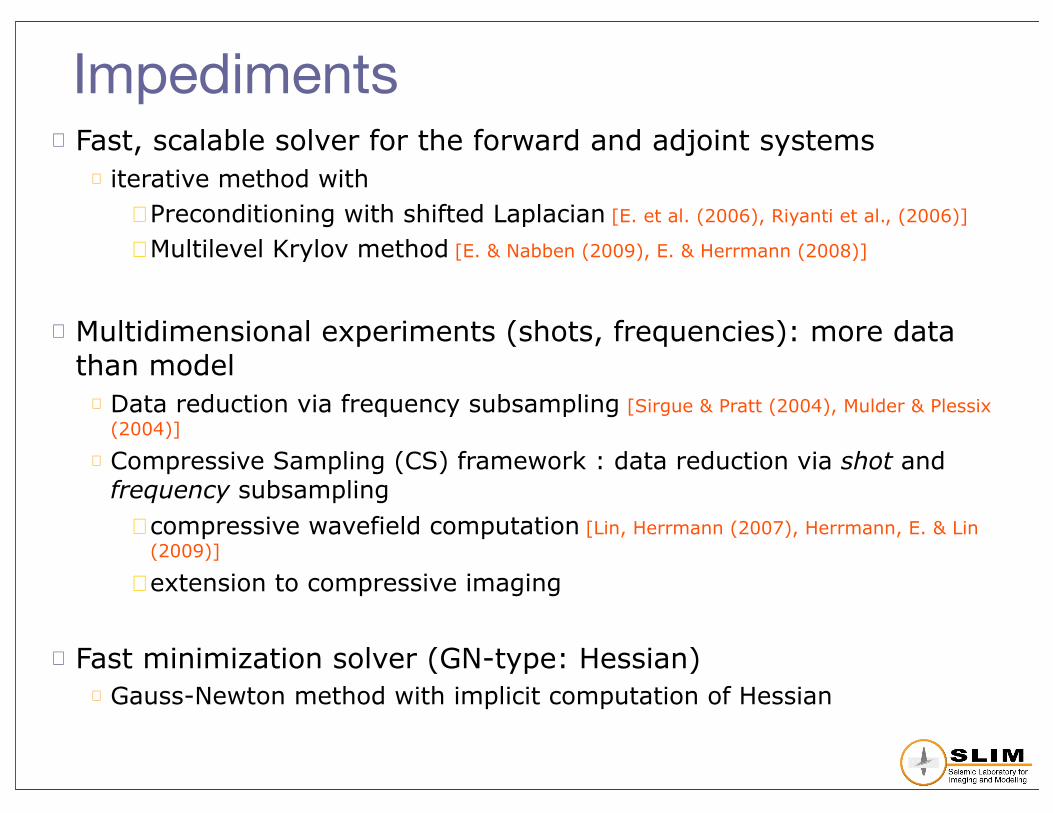
Impediments� Fast, scalable solver for the forward and adjoint systems

� iterative method with�Preconditioning with shifted Laplacian [E. et al. (2006), Riyanti et al., (2006)]

�Multilevel Krylov method [E. & Nabben (2009), E. & Herrmann (2008)]

� Multidimensional experiments (shots, frequencies): more data than model� Data reduction via frequency subsampling [Sirgue & Pratt (2004), Mulder & Plessix

(2004)]

� Compressive Sampling (CS) framework : data reduction via shot and frequency subsampling�compressive wavefield computation [Lin, Herrmann (2007), Herrmann, E. & Lin

(2009)]

�extension to compressive imaging

� Fast minimization solver (GN-type: Hessian)� Gauss-Newton method with implicit computation of Hessian

Our solution� Gauss-Newton with implicit Hessian (Gauss-Newton-Krylov, GNK)

� Dimensionality reduction � [Herrmann, E. & Lin (2009)]� [Tim Lin: Compressive simultaneous full-waveform simulation, this meeting, SM1]

� FWI with CS

!"""#

"""$

Q = D! s%&'(single shots

HU = Q

y = RMDU

!"

!"""#

"""$

Q = D! RMs% &' (simul. shots

HU = Q

y = DU

FWI with CS

The misfit functional:

with a CS-sampling matrix (reduces data size).

Optimization Problem: Find

subject to F[m] = DU[m]

E[m] =12!RM(P" F[m])!2

2

m̂ = arg minm!M

E[m]

RM

Main contribution: [Hermann et al. (2009), EAGE]

In line with this:

Sampling of overdetermined systems [Drineas, Mahoney & Muthukhrisnan (2006)]

� but is a bounded approximation.

See also: Krebs et al. (2009), this meeting

E[m] =12!P" F[m]!2

2

minE != minE

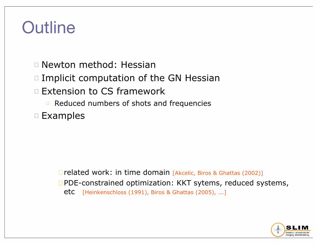
Outline

� Newton method: Hessian� Implicit computation of the GN Hessian � Extension to CS framework

� Reduced numbers of shots and frequencies

� Examples

�related work: in time domain [Akcelic, Biros & Ghattas (2002)]

�PDE-constrained optimization: KKT sytems, reduced systems, etc [Heinkenschloss (1991), Biros & Ghattas (2005), ...]

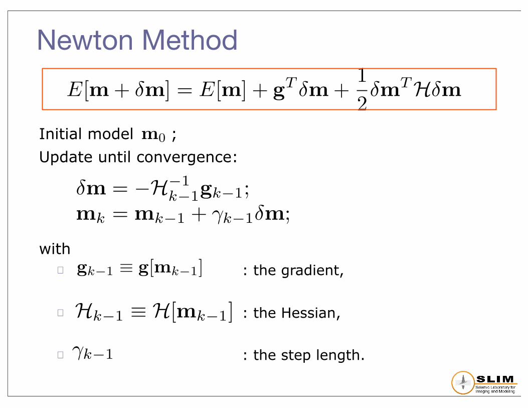
Newton Method

Initial model ;

Update until convergence:

with� : the gradient,

� : the Hessian,

� : the step length.

m0

gk!1 ! g[mk!1]

Hk!1 ! H[mk!1]

!k!1

E[m + !m] = E[m] + gT !m +12!mTH!m

mk = mk!1 + !k!1"m;!m = !H!1

k!1gk!1;

Hessian: with

� Negative sign: not necessarily SP(S)D

� Fast/quadratic convergence only if close to the minimizer

� From the adjoint system: (back-propagated)

H = [hi,j ]

hi,j =!

!mi

!!E

!mj

"

= rowsum!

!2U!mi!mj

! !U!mi

!F!mj

".

!U!mi

! V

� Simplify the Hessian by setting

� nonlinear wave phenomena (e.g. multiples)

� Giving

� This is associated with setting the back-propagated

wavefield in the Hessian

� is SP(S)D.

V = 0

Gauss-Newton Method!U!mi

!F!mj

= 0

hGNi,j = rowsum

!!2U

!mi!mj

".

HGN = [hGNi,j ]

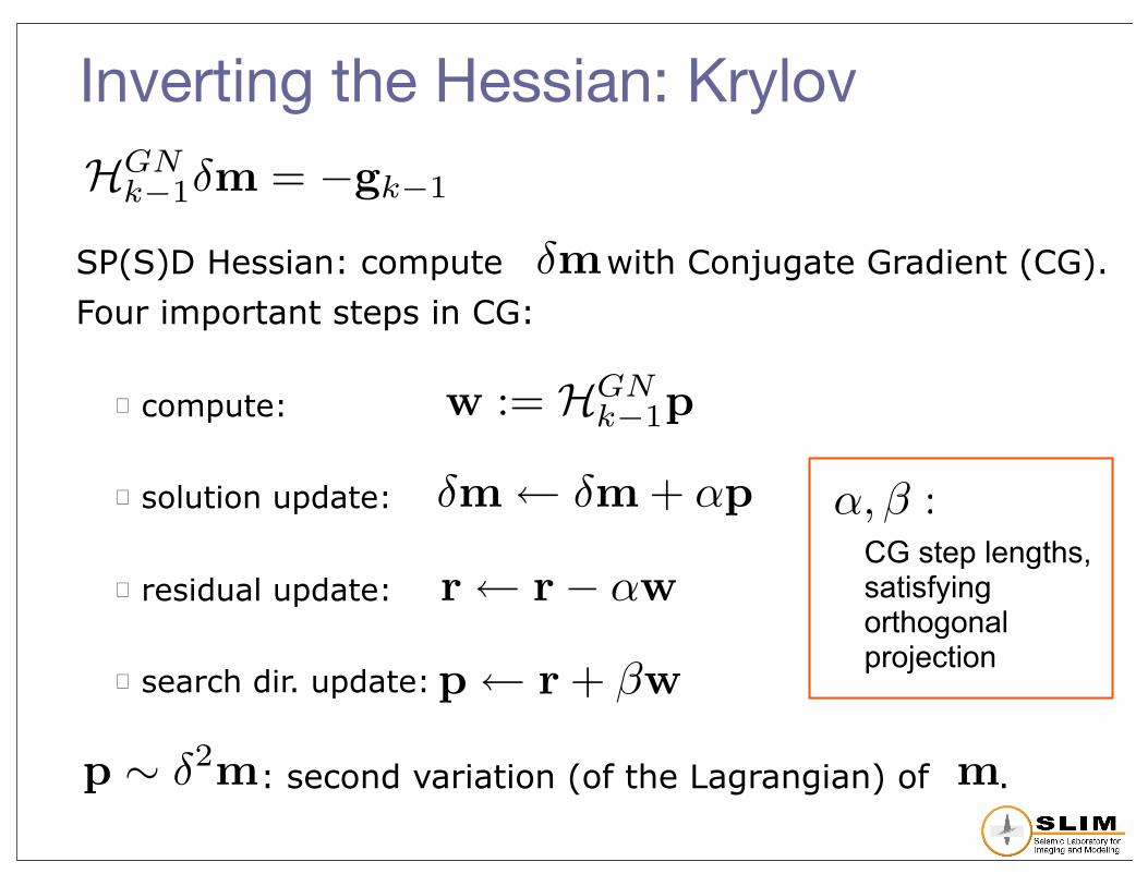
Inverting the Hessian: Krylov

SP(S)D Hessian: compute with Conjugate Gradient (CG).

Four important steps in CG:

� compute:

� solution update:

� residual update:

� search dir. update:

: second variation (of the Lagrangian) of .

HGNk!1!m = !gk!1

!m

!m! !m + "p

w := HGNk!1p

p ! !2m m

CG step lengths,satisfying orthogonal projection

!, " :

r! r" !w

p! r + !w

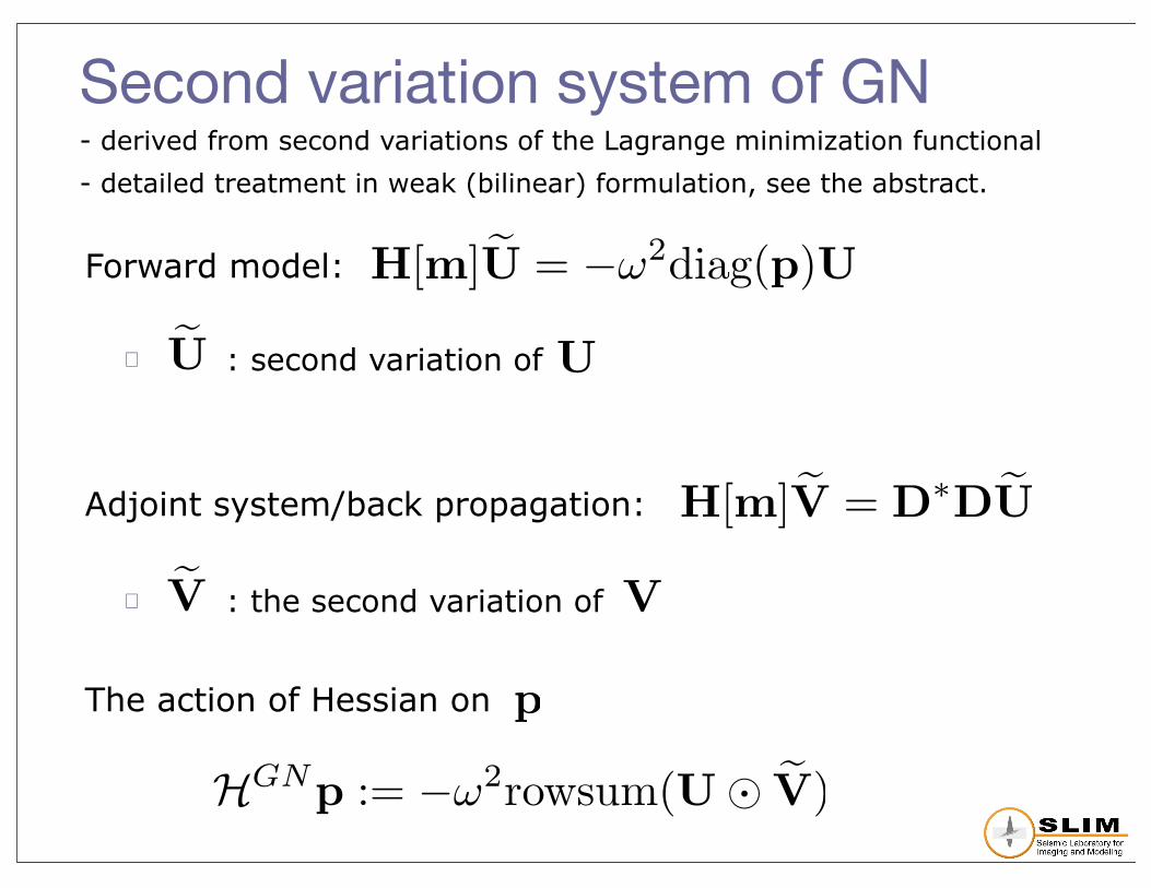
Forward model:

� : second variation of

Adjoint system/back propagation:

� : the second variation of

The action of Hessian on

Second variation system of GN

!U U

!V V

H[m]!U = !!2diag(p)U

- derived from second variations of the Lagrange minimization functional

- detailed treatment in weak (bilinear) formulation, see the abstract.

HGNp := !!2rowsum(U" !V)

p

H[m]!V = D!D!U

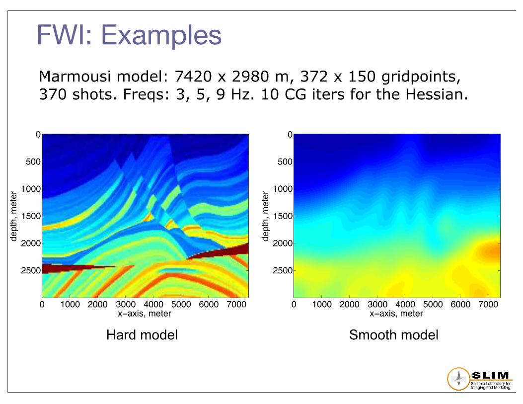
FWI: ExamplesMarmousi model: 7420 x 2980 m, 372 x 150 gridpoints, 370 shots. Freqs: 3, 5, 9 Hz. 10 CG iters for the Hessian.

x−axis, meter

dept

h, m

eter

0 1000 2000 3000 4000 5000 6000 7000

0

500

1000

1500

2000

2500

Hard model Smooth model

x−axis, meter

dept

h, m

eter

0 1000 2000 3000 4000 5000 6000 7000

0

500

1000

1500

2000

2500

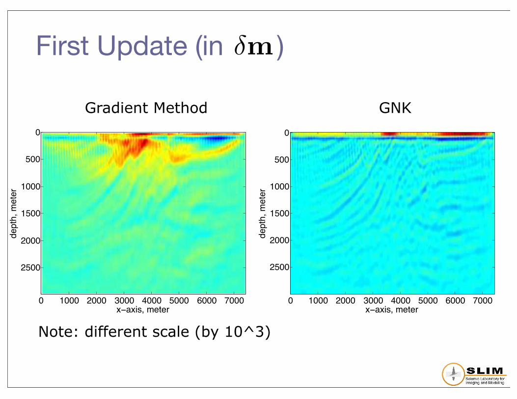
First Update (in )

Gradient Method GNK

Note: different scale (by 10^3)

!m

x−axis, meter

dept

h, m

eter

0 1000 2000 3000 4000 5000 6000 7000

0

500

1000

1500

2000

2500

x−axis, meter

dept

h, m

eter

0 1000 2000 3000 4000 5000 6000 7000

0

500

1000

1500

2000

2500

Velocity after the first update

Gradient Method GNK

x−axis, meter

dept

h, m

eter

0 1000 2000 3000 4000 5000 6000 7000

0

500

1000

1500

2000

2500

x−axis, meter

dept

h, m

eter

0 1000 2000 3000 4000 5000 6000 7000

0

500

1000

1500

2000

2500

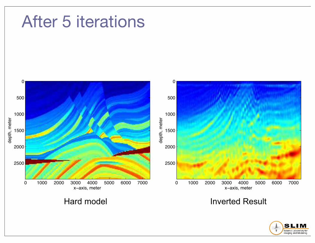
After 5 iterations

x−axis, meter

dept

h, m

eter

0 1000 2000 3000 4000 5000 6000 7000

0

500

1000

1500

2000

2500

x−axis, meter

dept

h, m

eter

0 1000 2000 3000 4000 5000 6000 7000

0

500

1000

1500

2000

2500

Hard model Inverted Result

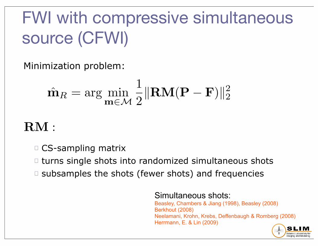
FWI with compressive simultaneous source (CFWI)

Minimization problem:

� CS-sampling matrix� turns single shots into randomized simultaneous shots� subsamples the shots (fewer shots) and frequencies

RM :

m̂R = arg minm!M

12!RM(P" F)!2

2

Simultaneous shots:Beasley, Chambers & Jiang (1998), Beasley (2008)Berkhout (2008)Neelamani, Krohn, Krebs, Deffenbaugh & Romberg (2008)Herrmann, E. & Lin (2009)

Gradient method of CFWI

Minimize functional:

Gradient update:

with the Jacobian .

E =12!RM(P"DU)!2

2

=12(RM(P"DU))T RM(P"DU)

gR = rowsum!JT (RM(P!DU))

"

J ! J(RMDU)

gR = !rowsum!J" (RM(P!DU))

"

Using wavefield-source equivalence [Herrmann, E., & Lin, 2009]

Gradient update

with

� : the (compressed) Jacobian w.r.t. to the

compressed simultaneous sources

� : data obtained with simultaneous shotP

!m = g = JT (P!DU)

J ! J(DU)

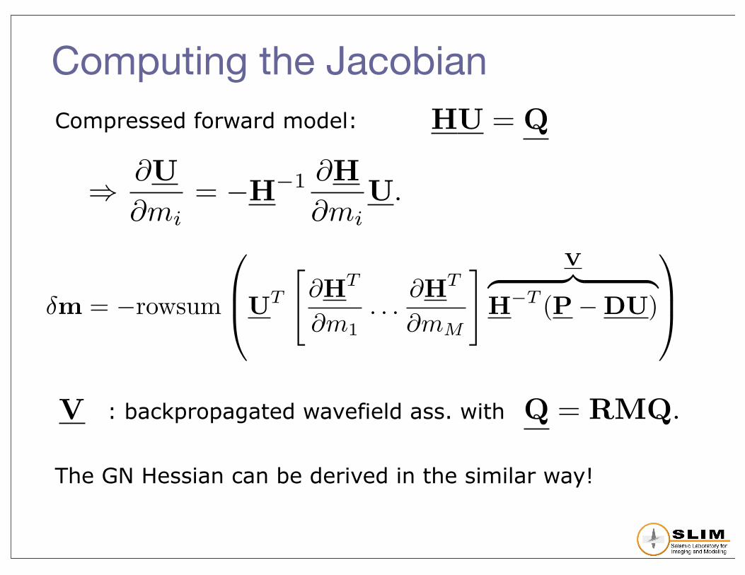
Computing the JacobianCompressed forward model:

: backpropagated wavefield ass. with

The GN Hessian can be derived in the similar way!

! !U!mi

= "H!1 !H!mi

U.

V Q = RMQ.

HU = Q

!m = !rowsum

!

"#UT

$"HT

"m1. . .

"HT

"mM

% V& '( )H!T (P!DU)

*

+,

Complexity Analysis

Gauss-Newton-Krylov (GNK)� Gradient : forward + back-propagation

� Hessian : forward + back-propagation per CG iteration

� Overall :

Compressive FWI with GNK:

Construction of negligible compared to FWI

nfnsn2 log n

nCGnfnsn2 log n

nCGnfnsn2 log n

nCGn!fn!

sn2 log n

n!s ! ns

RM

n!f ! nf ,

CFWI: Examples, GNK Iter #1 90% subsampled 37 randomized simul. shots 37 periodic shots

Noisy image --> recover the image via sparsity promoting

x−axis, meter

dept

h, m

eter

0 1000 2000 3000 4000 5000 6000 7000

0

500

1000

1500

2000

2500

x−axis, meter

dept

h, m

eter

0 1000 2000 3000 4000 5000 6000 7000

0

500

1000

1500

2000

2500

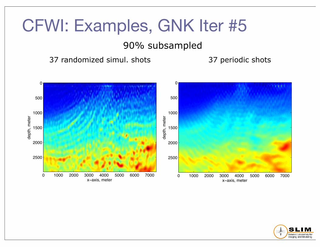
CFWI: Examples, GNK Iter #5 90% subsampled 37 randomized simul. shots 37 periodic shots

x−axis, meter

dept

h, m

eter

0 1000 2000 3000 4000 5000 6000 7000

0

500

1000

1500

2000

2500

x−axis, meter

dept

h, m

eter

0 1000 2000 3000 4000 5000 6000 7000

0

500

1000

1500

2000

2500

CFWI: Examples, GNK Iter #1 99% subsampled 4 randomized simul. shots 4 periodic shots

x−axis, meter

dept

h, m

eter

0 1000 2000 3000 4000 5000 6000 7000

0

500

1000

1500

2000

2500

x−axis, meter

dept

h, m

eter

0 1000 2000 3000 4000 5000 6000 7000

0

500

1000

1500

2000

2500

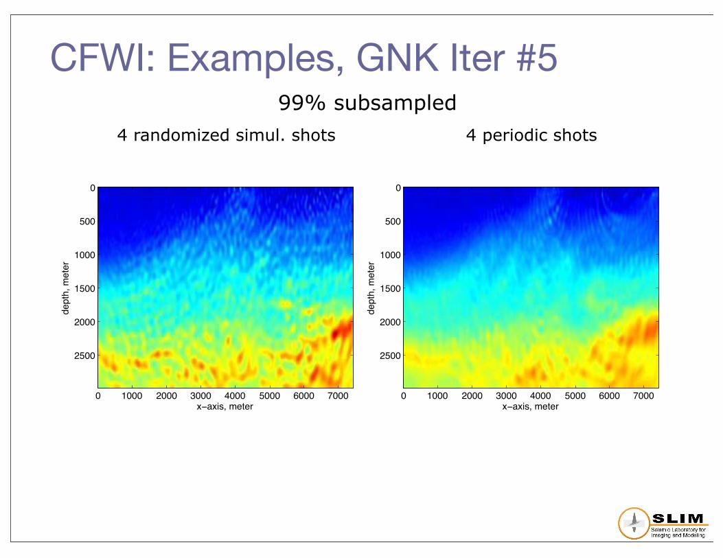
CFWI: Examples, GNK Iter #5 99% subsampled 4 randomized simul. shots 4 periodic shots

x−axis, meter

dept

h, m

eter

0 1000 2000 3000 4000 5000 6000 7000

0

500

1000

1500

2000

2500

x−axis, meter

dept

h, m

eter

0 1000 2000 3000 4000 5000 6000 7000

0

500

1000

1500

2000

2500

Conclusion�Viable inversion of GN Hessian with Krylov method� Accuracy of the inversion of Hessian depends on the number of

iterations --> better FWI result� Faster convergence of CG by preconditioners

�Implicit BFGS-type preconditioner�Curvelet-based preconditioner [Herrmann, Brown, E. & Moghaddam (2009)]

� Memory-friendly algorithm (gradient and Hessian can be computed on the fly)

� With scalable implicit solver for forward and adjoint systems, matrix-free algorithm [E., Oosterlee & Vuik (2006), E. & Nabben (2009), E. & Herrmann (2008)]

�Natural extension to compressive FWI� Similar results but less computational work� In the CS framework: l1 inversion

Acknowledgments

This work was in part financially supported by the Natural Sciences and Engineering Research Council of Canada Discovery Grant (22R81254) and the Collaborative Research and Development Grant DNOISE (334810-05) of Felix J. Herrmann.

This research was carried out as part of the SINBAD II project with support from the following organizations: BG Group, BP, Petrobras, and Schlumberger. 

Further information: slim.eos.ubc.ca