Frode Kristian Hansen- Data Analysis of the Cosmic Microwave Background
216
Data Analysis of the Cosmic Microwave Background. Dissertation der Fakult¨ at f¨ ur Physik der Ludwig-Maximilians-Universit¨ at M¨ unchen vorgelegt von: Frode Kristian Hansen aus Tønsber g M¨ unchen, den 11.01.2002
Transcript of Frode Kristian Hansen- Data Analysis of the Cosmic Microwave Background

8/3/2019 Frode Kristian Hansen- Data Analysis of the Cosmic Microwave Background
http://slidepdf.com/reader/full/frode-kristian-hansen-data-analysis-of-the-cosmic-microwave-background 1/216
Data Analysis
of
the Cosmic Microwave Background.
Dissertation der Fakultat fur Physik
der
Ludwig-Maximilians-Universitat Munchen
vorgelegt von: Frode Kristian Hansen
aus Tønsberg
Munchen, den 11.01.2002

8/3/2019 Frode Kristian Hansen- Data Analysis of the Cosmic Microwave Background
http://slidepdf.com/reader/full/frode-kristian-hansen-data-analysis-of-the-cosmic-microwave-background 2/216
i

8/3/2019 Frode Kristian Hansen- Data Analysis of the Cosmic Microwave Background
http://slidepdf.com/reader/full/frode-kristian-hansen-data-analysis-of-the-cosmic-microwave-background 3/216
Data Analysis
of
the Cosmic Microwave Background.
Dissertation der Fakultat fur Physik
der
Ludwig-Maximilians-Universitat Munchen
vorgelegt von: Frode Kristian Hansen
aus Tønsberg
Munchen, den 11.01.2002

8/3/2019 Frode Kristian Hansen- Data Analysis of the Cosmic Microwave Background
http://slidepdf.com/reader/full/frode-kristian-hansen-data-analysis-of-the-cosmic-microwave-background 4/216
1.Gutachter: Prof. S. White
2.Gutachter: Prof. A. Schenzle
Tag der Mundlichen Prufung: 12.06.02
i

8/3/2019 Frode Kristian Hansen- Data Analysis of the Cosmic Microwave Background
http://slidepdf.com/reader/full/frode-kristian-hansen-data-analysis-of-the-cosmic-microwave-background 5/216
Contents
Einleitung und Zusammenfassung . . . . . . . . . . . . . . . . . . 1Introduction and Summary . . . . . . . . . . . . . . . . . . . . . . 5
1 The Physics of the CMB fluctuation 9
1.1 Basic Concepts . . . . . . . . . . . . . . . . . . . . . . . . . . . . 101.1.1 The Friedmann Equations . . . . . . . . . . . . . . . . . . 101.1.2 Problems in Standard Cosmology . . . . . . . . . . . . . . 14
1.2 Theories of the Early Universe . . . . . . . . . . . . . . . . . . . . 161.2.1 Inflation . . . . . . . . . . . . . . . . . . . . . . . . . . . . 161.2.2 Cosmic Strings . . . . . . . . . . . . . . . . . . . . . . . . 19
1.3 The Growth of Perturbations in the Early Universe . . . . . . . . 201.3.1 Linear Evolution . . . . . . . . . . . . . . . . . . . . . . . 201.3.2 Nonlinear Evolution . . . . . . . . . . . . . . . . . . . . . 251.3.3 The Matter Power Spectrum . . . . . . . . . . . . . . . . . 26
1.4 The Recombination Era and the CMB . . . . . . . . . . . . . . . 281.4.1 The Origin of the CMB Anisotropies . . . . . . . . . . . . 291.4.2 The CMB Power Spectrum . . . . . . . . . . . . . . . . . . 321.4.3 Reionization and Secondary Anisotropies . . . . . . . . . . 38
1.4.4 Polarisation of the CMB and Tensor Perturbations . . . . 39
2 The Analysis of CMB Data 45
2.1 CMB Experiments, the Past, Present and Future . . . . . . . . . 452.1.1 COBE . . . . . . . . . . . . . . . . . . . . . . . . . . . . . 462.1.2 BOOMERANG . . . . . . . . . . . . . . . . . . . . . . . . 462.1.3 MAP . . . . . . . . . . . . . . . . . . . . . . . . . . . . . . 472.1.4 Planck . . . . . . . . . . . . . . . . . . . . . . . . . . . . . 492.1.5 Other Experiments . . . . . . . . . . . . . . . . . . . . . . 52
2.2 The Analysis of CMB Data Sets . . . . . . . . . . . . . . . . . . . 532.2.1 Map Making . . . . . . . . . . . . . . . . . . . . . . . . . . 53
2.2.2 Foregrounds . . . . . . . . . . . . . . . . . . . . . . . . . . 582.3 Power Spectrum Estimation . . . . . . . . . . . . . . . . . . . . . 62
2.3.1 Likelihood Estimation . . . . . . . . . . . . . . . . . . . . 632.3.2 Quadratic Estimators . . . . . . . . . . . . . . . . . . . . . 682.3.3 Two New Methods for Power Spectrum Estimation . . . . 70
ii

8/3/2019 Frode Kristian Hansen- Data Analysis of the Cosmic Microwave Background
http://slidepdf.com/reader/full/frode-kristian-hansen-data-analysis-of-the-cosmic-microwave-background 6/216
3 Fast Exact Power Spectrum Analysis for a Special Type of Scan-
ning Strategies 71
3.1 Fast Fourier Space Convolution . . . . . . . . . . . . . . . . . . . 723.2 Power Spectrum Estimation Using Scanning Rings . . . . . . . . . 76
3.2.1 Theory . . . . . . . . . . . . . . . . . . . . . . . . . . . . . 803.2.2 An Example . . . . . . . . . . . . . . . . . . . . . . . . . . 86
3.2.3 Discussion . . . . . . . . . . . . . . . . . . . . . . . . . . . 91
4 Gabor Transforms on the Sphere and Application to CMB Anal-
ysis 95
4.1 The Gabor Transformation and the Temperature Power Spectrum 974.1.1 The One Dimensional Gabor Transform . . . . . . . . . . 974.1.2 Gabor Transform on the Sphere . . . . . . . . . . . . . . . 984.1.3 Rotational Invariance . . . . . . . . . . . . . . . . . . . . . 108
4.2 Likelihood Analysis . . . . . . . . . . . . . . . . . . . . . . . . . . 1104.2.1 The Form of the Likelihood Function . . . . . . . . . . . . 1104.2.2 The Correlation Matrix . . . . . . . . . . . . . . . . . . . . 114
4.2.3 Including White Noise . . . . . . . . . . . . . . . . . . . . 1164.2.4 Likelihood Estimation and Results . . . . . . . . . . . . . 119
4.3 Extensions of the Method . . . . . . . . . . . . . . . . . . . . . . 1344.3.1 Multiple Patches . . . . . . . . . . . . . . . . . . . . . . . 1354.3.2 Monte Carlo Simulations of the Noise Correlations and Ex-
tention to Correlated Noise . . . . . . . . . . . . . . . . . 1444.4 Discussion . . . . . . . . . . . . . . . . . . . . . . . . . . . . . . . 147
5 Gabor Transform on the Polarised CMB Sky 149
5.1 The Gabor Transformation . . . . . . . . . . . . . . . . . . . . . . 1505.1.1 Polarisation Powerspectra . . . . . . . . . . . . . . . . . . 1505.1.2 Rotational Invariance . . . . . . . . . . . . . . . . . . . . . 170
5.2 Likelihood Analysis . . . . . . . . . . . . . . . . . . . . . . . . . . 1715.2.1 The Form of the Likelihood Function for Polarisation . . . 1715.2.2 The Polarisation Correlation Matrix . . . . . . . . . . . . 1785.2.3 Polarisation with Noise . . . . . . . . . . . . . . . . . . . . 182
5.3 Results of Likelihood Estimations . . . . . . . . . . . . . . . . . . 1865.4 Discussion . . . . . . . . . . . . . . . . . . . . . . . . . . . . . . . 187
A Rotation Matrices 191
B Spin-s Harmonics 192
C Some Wigner Symbol Relations 193
D Recurrence Relation 194
iii

8/3/2019 Frode Kristian Hansen- Data Analysis of the Cosmic Microwave Background
http://slidepdf.com/reader/full/frode-kristian-hansen-data-analysis-of-the-cosmic-microwave-background 7/216
E Extention of the Recurrence Relation to Polarisation 197
Acknowledgements . . . . . . . . . . . . . . . . . . . . . . . . . . 205Lebenslauf . . . . . . . . . . . . . . . . . . . . . . . . . . . . . . . 206
iv

8/3/2019 Frode Kristian Hansen- Data Analysis of the Cosmic Microwave Background
http://slidepdf.com/reader/full/frode-kristian-hansen-data-analysis-of-the-cosmic-microwave-background 8/216
v
8/3/2019 Frode Kristian Hansen- Data Analysis of the Cosmic Microwave Background
http://slidepdf.com/reader/full/frode-kristian-hansen-data-analysis-of-the-cosmic-microwave-background 9/216
Einleitung und Zusammenfassung 1
Einleitung und Zusammenfassung
Das fruhe Universum bestand aus einem heißen, dichten und ionisierten Gas aus
Elektronen, Protonen, Neutronen, einigen leichten Atomkernen und Photonen.Das Universum war in dieser Zeit optisch dicht da aufgrund der haufigen Zusam-menstosse mit Elektronen in dem dichten Gas, die Photonen sich nicht sehr weitbewegen konnten. Die Temperatur war so hoch, dass die Elektronen, Protonenund Neutronen nicht zu Atomen rekombinieren konnten. Als das Universum ex-pandierte, kuhlte es sich ab. Ungefahr 300 000 Jahre nach dem Urknall betrugdie Temperatur des Gases etwa 3000 Grad Kelvin. Unterhalb dieser Temper-atur ist die Bildung der ersten Atome des Universums moglich. Die Elektronenund Protonen rekombinierten zu Atomen. Im Allgemeinen ist die Wahrschein-lichkeit dafur, dass ein Photon mit einem Atom zusammenstoßt, viel geringer alsdie Wahrscheinlichkeit dafur, dass es mit freien Elektronen oder Protonen kolli-
diert. Aus diesem Grund sagt man, dass das Universum durchsichtich wurde, alsdie Elektronen mit den Protonen rekombinierten. Die Photonen bewegten sichentlang einer Geraden ohne dass sie abgelenkt wurden. Ungefahr 12 MilliardenJahre spater trafen die Photonen einen Detektor auf einem Planeten names ‘dieErde’ und gaben den Wissenschaftlern wertvolle Informationen uber den Anfangdes Universums. Diese Strahlung, die auf ihrer Reise von den fruhesten Zeitenbis heute kaum eine Veranderung erfahren hat, wird ’der kosmische Mikrowellen-hintergrund’ genannt, und ist das Thema dieser Doktorarbeit.
Das dichte Gas des fruhen Universums war nicht ganz homogen. Prozesseder ersten 10−34 Sekunden nach dem Urknall verursachten kleine Schwankun-gen in der Dichte. Die Entwicklung dieser Schwankungen unter dem Einfluss vonGravitation und Druck kann man mit Hilfe der Hydrodynamik einfach berechnen.Nachdem das Universum durchsichtich wurde (Rekombination), entwickelten sichdie Schwankungen und sind heute als Sterne, Galaxien und Galaxienhaufen sicht-bar. Die Bildung dieser Objekte ist eine sehr komplizierte Prozess, die nochnicht vollstandig verstanden ist. Die Entwicklung der Strukturen des Universumsbevor Rekombination kann man mit linearer Physik beschreiben. Hatte man dieMoglichkeit, das Universum in diesem fruheren Stadium zu beobachten, hatteman Informationen uber die Eigenschaften und Anfang des Universums auf eineeinfache Weise erhalten konnen. Der kosmische Mikrowellenhintergrund (CMB)
gibt eine solche Moglichkeit. Diese Strahlung ist vom Zeitpunkt der Rekombina-tion bis heute nahezu ohne Stohrung gereist und ist somit ein Bild vom Universumund der Verteilung der Dichteschwankungen zu diesem Zeitpunkt.
Der CMB wurde zuerst von Penzias und Wilson 1965 als isotrope Schwarzkorper-

8/3/2019 Frode Kristian Hansen- Data Analysis of the Cosmic Microwave Background
http://slidepdf.com/reader/full/frode-kristian-hansen-data-analysis-of-the-cosmic-microwave-background 10/216
Einleitung und Zusammenfassung 2
strahlung mit einer Temperatur von ca. 2.7 Grad Kelvin entdeckt. Wie obenerwahnt war die Temperatur des Gases zum Zeitpunkt der Rekombination ca.3000 Grad Kelvin, da das Universum aber seitdem ungefahr 1000 mal großergeworden ist, ist die Temperatur dieser Schwarzkorperstrahlung auch genau umdiesen Faktor kleiner geworden. Die Schwankungen der Dichte des Universumszur Zeit der Rekombination verursachten kleine Unregelmaßigkeiten in der Tem-
peratur des CMB, die zuerst 1992 mit dem Cosmic Background Explorer (COBE)Satellit entdeckt wurden. In den letzen Jahren sind mehrere Experimente mit im-mer hoherer raumlicher Auflosung von der Erde und von Ballons aus durchgefuhrtworden. Diese Experimente haben schon wertvolle Informationen uber das fruheUniversum gegeben. Ein anderer Satellit namens MAP fuhrt jetzt Beobachtungendes CMB durch und der Planck Satellit, der in einigen Jahren ins All geschicktwird, wird Beobachtungen mit noch hoherer raumlicher und spektraler Auflosungdurchfuhren.
Da die Experimente immer hohere Auflosung erreichen und immer großereTeile des Himmels beobachten, wird es auch immer schwieriger, die Daten zuanalysieren. Die Analyse der Daten jetziger Experimente ist bereits ein Problemund die Menge der Daten von MAP und Planck werden um ein Vielfaches großersein. Die Standardmethode, um Informationen (kosmologische Parametern) ausCMB Daten zu extrahieren ist die Maximum-Likelihood Methode. Diese Meth-ode fordert die Invertierung einer N × N Matrix, wobei N die Anzahl der Pixeleines Experimentes ist. Diese Invertierung erfordert N 3 Berechnungen. Fur dasPlanck Experiment wird N einen Wert von mehr als zehn Millionen haben. DieInvertierung einer Matrix dieser Große dauert mehrere Tausend Jahre mit denschellsten Supercomputern. Daher muss man andere Methoden finden um dieDaten analysieren zu konnen. In dieser Doktorarbeit werde ich zwei neue Meth-
oden prasentieren, die es ermoglichen, CMB Daten schnell zu analysieren. Mitdiesen Methoden wird man das CMB Leistungsspektrum -die spharisch harmonis-chen Koeffizienten der CMB Temperatur Daten- schnell extrahieren konnen. MitHilfe des Leistungsspektrums kann man die kosmologischen Parametern einfachberechnen.
In Kapitel (1) wird die Physik des fruhen Universums beschrieben. EineZusammenfassung der Entstehung und der Entwicklung der Strukturen des Uni-versums vom Urknall bis heute wird prasentiert. Die physikalischen Prozesse,die die Hintergrundstrahlung verursacht haben, werden zusammengefasst, und eswird gezeigt, wie diese Prozesse eine Abhangigkeit des Leistungsspektrums vonden kosmologischen Parametern verursachen. In Kapitel (2) wird einen Uberblickuber vergangenen, heutigen und zukunftigen CMB Experimente gegeben, unddie Standardmethoden fur Analyse der CMB Daten werden erlautert. In diesemKapitel wird auch beschrieben, wie man eine CMB Karte von den ‘ZeitgeordnetenDaten’ (TOD) eines CMB Experimentes macht und wie man Storungen durch

8/3/2019 Frode Kristian Hansen- Data Analysis of the Cosmic Microwave Background
http://slidepdf.com/reader/full/frode-kristian-hansen-data-analysis-of-the-cosmic-microwave-background 11/216
Einleitung und Zusammenfassung 3
die Mikrowellenstrahlung anderer Korper entfernen kann. Zum Schluss des Kapi-tels werden die neusten Methoden fur die Extraktion des Leistungsspektrums ausCMB Daten beschrieben.
In Kapitel (3) wird beschrieben, wie man mit einer Maximum-Likelihood-Methode das Leistungsspektrum direkt von den TOD extrahieren kann, ohne
zuerst eine CMB Karte zu erstellen. Diese Methode ist auf Experimente wieMAP und Planck anwendbar die den Himmel ‘in Ringen von Ringen’ vermessen.Symmetrien dieser Abtastmethode machen die Korrelationsmatrizen fur Signalund Storung blockdiagonal im Fourierraum. Aus diesem Grund kann man dieKorrelationsmatrix mit N 2 Berechnungen statt N 3 invertieren. Das ermoglichtdie Verwendung der Maximum-Likelihood Methode fur solche Experimente. Weilwirkliche Experimente, Schwankungen von der hier angenommenen idealen Ab-tastmethode haben werden, werden Erweiterungen dieser Methode fur solche Ex-perimente diskutiert.
In Kapitel (4) wird eine andere Methode mit der man das Leistungsspektrumvon CMB Daten schnell extrahieren kann, vorgestellt. In diesem Kapitel wirdauch erlautert wie man ’Windowed Fourier Transforms’ (auch als ’Gabor Trans-forms’ bekannt) vom Eindimensionalen auf die 2-dimensionale Kugeloberflacheerweitert. Es wird gezeigt, wie man das Leistungsspektrum von einem Ausschnittdes Himmels (Pseudo-Leistungsspektrum) als Eingangsdaten fur eine Maximum-Likelihood Analyse verwenden kann. Die Korrelationsmatrix der Maximum-Likelihood Methode ist in diesem Fall viel kleiner als wenn alle Pixeln einesExperimentes benutzt werden. Aus diesem Grund ist die Invertierung der Ma-trix schnell. Es wird gezeigt, dass die Annahme einer Gaußschen Verteilung derPseudo-Leistungsspektrumskoeffizienten eine gute Annahrung ist. Es wird auch
gezeigt, wie man CMB Daten vom ganzen Himmel analysieren kann, wenn manden Himmel in viele kleinere Ausschnitte aufteilt und alle Ausschnitte gleichzeitiganalysiert. In Kapitel (5) wird die Methode fur Analyse der CMB PolarisationDaten erweitert.

8/3/2019 Frode Kristian Hansen- Data Analysis of the Cosmic Microwave Background
http://slidepdf.com/reader/full/frode-kristian-hansen-data-analysis-of-the-cosmic-microwave-background 12/216
Einleitung und Zusammenfassung 4

8/3/2019 Frode Kristian Hansen- Data Analysis of the Cosmic Microwave Background
http://slidepdf.com/reader/full/frode-kristian-hansen-data-analysis-of-the-cosmic-microwave-background 13/216
Introduction and Summary 5
Introduction and Summary
The early universe consisted of a dense, hot and ionised gas of electrons, protons,
neutrons, some light atomic nuclei and photons. The universe at that time wasoptically thick as the photons could not travel very far before being scatteredon electrons in the dense gas. The temperature was too hot for the electronsto combine with the nuclei and form atoms. But as the universe expanded itcooled. About 300 000 years after the Big Bang, the temperature of the densegas filling the universe was about 3000 degree Kelvin. This temperature allowedthe formation of the first atoms in the universe. The electrons combined withthe protons to form atoms. The probability for a photon to scatter on a neutralatom is much less than the probability to scatter on free electrons and protons.For this reason it is said that the universe got transparent when the electronswere bound to the protons. The photons continued travelling in a straight line
without being scattered. About 12 billion years later some of these photons hit adetector on the planet called ‘the earth’. And it provided scientists with valuableinformation about the origin of the universe. This radiation which has travelledmore or less unchanged from the earliest times until today is called the cosmicmicrowave background radiation , and is the topic of this Ph.D. thesis.
The dense gas in the early universe was not completely homogeneous. Pro-cesses during the first 10−34 seconds after the Big Bang created small densityfluctuations. The evolution of these fluctuations under the influence of gravita-tion and pressure in the dense gas can be easily calculated using hydrodynamics.After the universe became transparent (known as ‘the recombination era’), thesesmall density fluctuations evolved to be the structure that can be seen in thepresent universe, stars, galaxies and clusters of galaxies. The formation of theseobjects is physically very complicated and not completely understood. If onehad the possibility to observe the universe at an earlier stage when structureformation was still governed by known linear physics, it would be easier to gaininformation about the properties of the universe and its origin. The cosmic mi-crowave background (CMB) radiation provides such a possibility. The radiationhas travelled from the recombination epoch until today and gives a picture of theuniverse and the distribution of density fluctuations at the recombination epoch.
The CMB was first detected by Penzias and Wilson in 1965 as a black body ra-diation with a temperature of 2.7 Kelvin coming from all directions. As explainedabovem the temperature of the gas at recombination was about 3000 Kelvin, butsince that time the universe has expanded by a factor of roughly 1000 which hasdecreased the temperature of the CMB photons by a similar factor. The density
8/3/2019 Frode Kristian Hansen- Data Analysis of the Cosmic Microwave Background
http://slidepdf.com/reader/full/frode-kristian-hansen-data-analysis-of-the-cosmic-microwave-background 14/216
Introduction and Summary 6
fluctuations in the universe at the recombination epoch gave rise to small fluc-tuations in the CMB temperature. These fluctuations were first detected by theCosmic Background Explorer (COBE) satellite in 1992. In the recent years sev-eral ground and balloon borne experiments have made observations of the CMBat increasing angular resolution. These observations have already provided valu-able information about the early universe. Another satellite called Microwave
Anisotropy Probe (MAP) is currently observing the CMB and a satellite calledPlanck will make observations with an even higher angular and spectral resolu-tion in a few years. As the experiment are getting higher resolution and largersky coverage the task of analysing the data is gradually getting harder. Alreadythe analysis of the present datasets have presented a challenge and the datasetsfrom MAP and Planck will be several times larger. The standard method of extracting information in terms of cosmological parameters from the CMB datahas been the method of maximum-likelihood. Unfortunately this method requiresthe inversion of a N × N correlation matrix where N is the number of pixels inthe experiment. This takes of the order N 3 operations. For Planck N will be of the order of tens of millions and the inversion of the corresponding matrix takesthousands of years on the fastest supercomputers. Other methods for analysingthe data have to be found. The aim of this thesis is to present two new methodsto analyse CMB temperature and polarisation data. The methods described inthe thesis aim at extracting the angular power spectrum of the CMB which isthe spherical harmonic transform of the CMB sky. From this power spectrumthe cosmological parameters can be extracted.
In chapter (1) a description of the physics of the early universe is given. Asummary of the formation and evolution of structure from the Big Bang untilthe present era is presented. The processes giving rise to the CMB is also out-
lined and it is shown how these processes give a dependency on cosmologicalparameters in the angular power spectrum of the CMB. Then in chapter (2) thepast, present and future CMB experiments are reviewed and the standard meth-ods of data analysis are presented. The chapter also contains a description of the process of making a CMB sky map from the time ordered data (TOD) of a CMB experiment and the removing of foreground contamination. Finally thelast methods of extracting the angular power spectrum are reviewed.
In chapter (3) a new method is presented for extracting the CMB powerspectrum using the maximum-likelihood method directly on the TOD instead of making a CMB map first. The method is applicable to experiments scanning onrings of rings on the sky like the MAP and Planck experiments. Symmetries of this scanning strategy make the signal and noise correlation matrix for the likeli-hood calculation block diagonal in Fourier space. For this reason the matrix canbe inverted in N 2 operations instead of N 3. This makes the maximum-likelihoodmethod feasible for this kind of experiments. The method is exact and naturally

8/3/2019 Frode Kristian Hansen- Data Analysis of the Cosmic Microwave Background
http://slidepdf.com/reader/full/frode-kristian-hansen-data-analysis-of-the-cosmic-microwave-background 15/216
Introduction and Summary 7
takes into account arbitrary beam shapes and side lobes which other existingmethods can not deal with. As realistic experiments can have deviation fromthe ideal scanning strategy assumed, extensions of the method to these cases isdiscussed.
In chapter (4) a different approach of estimating the angular power spectrum
of the CMB is shown. In the chapter it will be explained how the windowedFourier transforms (known as Gabor transforms) can be extended from the lineto the sphere. It will be shown how one can take a patch on the CMB sky and usethe power spectrum of this patch (the so called pseudo power spectrum) as inputto a maximum-likelihood procedure. The correlation matrix for this likelihoodis much smaller than when using all the pixels of the experiment and matrix in-version is very fast. The assumption is that the coefficients of the pseudo powerspectrum is Gaussian distributed which is shown to be a good approximation.It is also shown how many such patches can be combined and in this way it ispossible to analyse datasets with observations of the full CMB sky by breakingthem up into several patches which are all analysed simultaneously. In chapter(5) the method is extended to CMB polarisation.

8/3/2019 Frode Kristian Hansen- Data Analysis of the Cosmic Microwave Background
http://slidepdf.com/reader/full/frode-kristian-hansen-data-analysis-of-the-cosmic-microwave-background 16/216
Introduction and Summary 8
8/3/2019 Frode Kristian Hansen- Data Analysis of the Cosmic Microwave Background
http://slidepdf.com/reader/full/frode-kristian-hansen-data-analysis-of-the-cosmic-microwave-background 17/216
Chapter 1
The Physics of the CMB
fluctuation
In this chapter I will discuss the physical processes that gave rise to the fluctu-ations in the Cosmic Microwave Background (CMB). I will start by introducing
some basic concepts in cosmology (sect. 1.1), and discuss some main problemsthat standard cosmology (sect. 1.1.2) is facing. In sect. 1.2.1 I will briefly discussthe theory of inflation in the early universe and show how this theory may solvesome of the problems in cosmology as well as explain the origin of structure in theuniverse. In sect. 1.2.2 an alternative theory of structure formation will brieflybe reviewed.
I will proceed by a description of how the density perturbation produced inthe early universe were growing. In the early stages, the evolution of primordialdensity perturbation were linear (sect. 1.3.1). In the last stages also nonlinear
effects became important (sect. 1.3.2). I will discuss the physics of the recombi-nation era where light decoupled from matter (sect. 1.4.1) and gave rise to theCMB. It will be shown that by studying the fluctuations in the CMB, one actu-ally studies the density fluctuations at the recombination epoch when structureformation was still governed by linear evolution. The density distribution in theuniverse today has undergone nonlinear evolution by physical processes that arenot completely known. For this reason it is easier to reconstruct the primordialfield of density fluctuations and to estimate the values of the cosmological pa-rameters from the spectrum of density fluctuations at the last scattering surface.How this can be done will be reviewed in sect. 1.4.2. In sect. 1.4.3 I will discusshow processes that took place after recombination also contributed to small scale
power in the CMB.
The discussion in sect. 1.1 and 1.2 are when no other references are given,built on the book (Kolb and Turner 1990) and the reviews (Watson 2000; Narlikarand Padmanabhan 1991). Section 1.3 mostly follows the books (Kolb and Turner
8/3/2019 Frode Kristian Hansen- Data Analysis of the Cosmic Microwave Background
http://slidepdf.com/reader/full/frode-kristian-hansen-data-analysis-of-the-cosmic-microwave-background 18/216
1.1 Basic Concepts 10
1990; Coles and Lucchin 1995) and the review (Padmanabhan 1999). The paper(Hu and Sugiyama 1995) and (Zaldariagga and Harari 1995) are the main sourcesfor section 1.4. All the power spectra used in this thesis were obtained using thepublicly available code CMBFAST (Seljak and Zeldariagga 1996). The code canbe found at the site http://physics.nyu.edu/matiasz/CMBFAST/cmbfast.html
1.1 Basic Concepts
In this section I will review the basic principles of cosmology (sect.1.1.1). ThenI will outline the main problems that the standard Big Bang scenario is facing(sect. 1.1.2).
1.1.1 The Friedmann Equations
The Cosmological Principle (CP), is the foundation of almost all modern cosmol-ogy. The CP consists of two parts,
1. Homogeneity: The universe is homogeneous on large scales
2. Isotropy: The universe is isotropic on large scales
The homogeneity principle says that the universe is supposed to look the sameat every point. The isotropy principle says that the universe is supposed to looksimilar in all directions. On small scales this is obviously not the case, but ob-servations indicate that this seems to be true on larger scales. One of the bestprobes is the CMB which has been observed to be isotropic to one part in 105.
The metric in a homogeneous and isotropic universe is the Friedmann-Robertson-Walker (FRW) metric,
ds2 = c2dt2 − a2(t)
dr2
1 − kr2+ r2dθ2 + r2 sin2 θdφ2
. (1.1)
Here, (r,θ,φ,t) are the comoving coordinates (coordinates moving with the ex-pansion of the universe). The expansion factor of the universe is a(t), and k isthe curvature. By a proper rescaling of the coordinates, k can take the values −1(hyperbolic space), 0 (flat space) or 1 (spherical space).
The goal now is to find the Friedmann equations, which are the ’equations of motion’ of the universe. This can be achieved by inserting the FRW metric intothe Einstein equations. The Einstein equations read
Rµν − 1
2gµν R +
Λgµν
c2= −8πG
c4T µν , (1.2)

8/3/2019 Frode Kristian Hansen- Data Analysis of the Cosmic Microwave Background
http://slidepdf.com/reader/full/frode-kristian-hansen-data-analysis-of-the-cosmic-microwave-background 19/216
1.1 Basic Concepts 11
where Rµν is the Ricci tensor, R is the Ricci scalar, Λ is the cosmological constant,gµν is the metric, G is the gravitational constant and T µν is the stress-energytensor of the universe. These quantities are described in more detail elsewhere(e.g. (Kolb and Turner 1990)). The left side of the equation contains terms whichare purely geometry dependent and the right side has all the matter and energyin it. The energy/matter content of the universe was very different at different
epochs, but a quite general form of the stress-energy tensor is that of a perfectfluid. In a perfect fluid T µν is diagonal and takes the form (I have set c = 1 forsimplicity),
T µν = diag(ρ, − p, − p, − p). (1.3)
Here ρ is the energy density and p is the pressure of the fluid.
So inserting the FRW metric (1.1) and the stress-energy tensor for a per-fect fluid (1.3) into the Einstein equations (1.2), one arrives at the Friedmannequations:
aa = −4πG3 (ρT + 3 pT ) , (1.4)
a2
a2=
8πGρT
3− k
a2. (1.5)
Here the dots denote derivatives with respect to time. The cosmological constantis included here, by letting
ρT = ρ + ρΛ, (1.6)
pT = p − ρΛ, (1.7)
where ρΛ
= Λ
8πG.

8/3/2019 Frode Kristian Hansen- Data Analysis of the Cosmic Microwave Background
http://slidepdf.com/reader/full/frode-kristian-hansen-data-analysis-of-the-cosmic-microwave-background 20/216
1.1 Basic Concepts 12
t
t
t
t
t
i
f
rec
eq
io
matter dominated era
radiation and matter decoupled
reionized universe
t 0
Planck era
inflation
radiation dominated era
vacuum energy dominated era
Figure 1.1: A sketch of the history of the universe (the time axis is not linear).
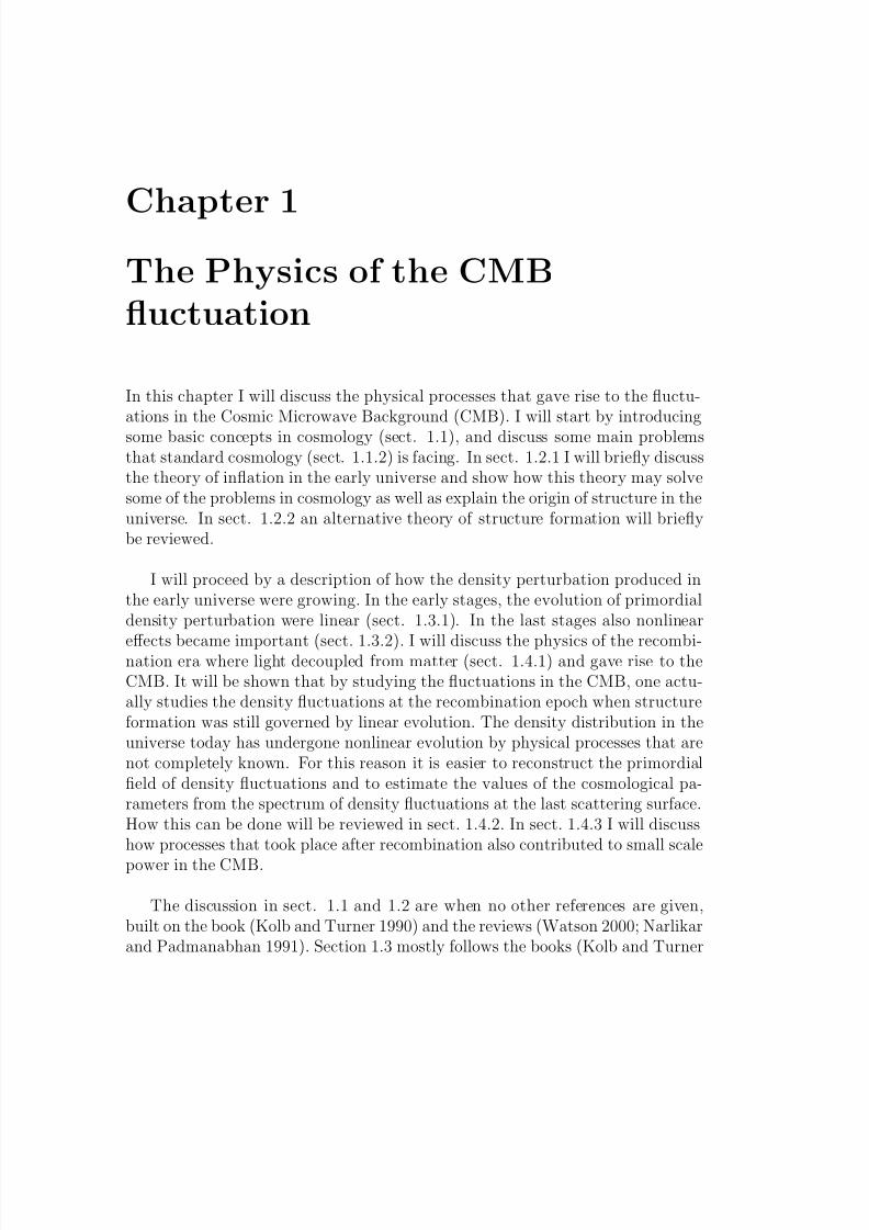
To show some applications of the Friedmann equations I will now concentrate
on two stages in the history of the universe. The radiation dominated era andthe matter dominated era . At cosmic time teq ≈ 104years the energy densitiesof matter and radiation in the universe were equal. Well before teq there wasan era when the energy density in the universe was dominated by radiation. Inthat epoch, the energy density due to radiation was much higher than the en-

8/3/2019 Frode Kristian Hansen- Data Analysis of the Cosmic Microwave Background
http://slidepdf.com/reader/full/frode-kristian-hansen-data-analysis-of-the-cosmic-microwave-background 21/216
1.1 Basic Concepts 13
ergy density due to matter, and one can use the equation of state for radiation p = αρ with α = 1/3. After teq, matter was dominating the energy density of the universe. In the matter dominated era one can neglect the pressure (α = 0).The matter dominated era includes the recombination epoch (trec ≈ 105years) atwhich matter and radiation decoupled. Recent observation indicate that thereis a cosmological constant (Jaffe et al. 2001) and that the universe at present
is dominated by vacuum energy (ρmatter/ρΛ ≈ 0.4). The equation of state of vacuum energy is α = −1. The history of the universe is sketched in figure (1.1).
First I will show how the energy density ρ in the universe is changing withthe scale factor a. To do this, one can combine equation (1.4) and (1.5) to get
d
da(ρa3) + 3a2 p − a2Λ
4πG= 0. (1.8)
Using the equation of state, one can rewrite this as
d
da(ρa3(1+α)) =a2+3αΛ
4πG . (1.9)
One easily sees that for the matter dominated era, ρ ∝ a−3 (actually ρ =k1a−3 + k2Λ where k1 and k2 are constants), for the radiation dominated eraρ ∝ a−4 and for the vacuum energy dominated epoch ρ ∝ ln a.
Using the Friedmann equations one can find how the expansion parametervaries with time. As a simple example I will just demonstrate the flat universecase with Λ = 0. In this case one can set ρ = k1a−3 for a matter dominateduniverse into equation (1.5) and integrate the equation. One sees that a ∝ t2/3.
Similarly for a radiation dominated universe one has a ∝√
t. In a radiationdominated universe, temperature T and density are related by ρ ∝ T 4 givingT ∝ t−1/2. With this relation one can study how the temperature in th universevaries with time in the early stages of the history of the universe.A similar argu-ment yields for the matter dominated universe T ∝ t−2/3.
I now define some new parameters, namely
• the Hubble constant
H =a(t)
a(t). (1.10)
• The redshift that one observes today from a given epoch t
z(t) =a0
a(t)− 1, (1.11)
where a0 = a(t0), where t0 is the present time.

8/3/2019 Frode Kristian Hansen- Data Analysis of the Cosmic Microwave Background
http://slidepdf.com/reader/full/frode-kristian-hansen-data-analysis-of-the-cosmic-microwave-background 22/216
1.1 Basic Concepts 14
• The density parameter Ω is defined as
Ω =ρ
ρc, (1.12)
where
• ρc is the critical density . This is the density at which the universe is exactlyflat (k = 0). This can be directly found from equation (1.5), setting k = 0and solving for the density ρT . This gives
ρc(t) =3H 2(t)
8πG. (1.13)
The critical density today is ρc ≈ 2 × 10⁻²⁹h2gcm−3 (where I used H 0 =H (t0) = h × 100kms−1Mpc−1).
Finally I will explain some expressions which will be useful. These are theparticle horizon , the event horizon and the Hubble radius.
• The particle horizon is the distance which limits the range of casual com-munications from the past. It is simply the most distant point from whichone can receive a light signal which was emitted at the beginning of theuniverse.
• Similarly the event horizon limits casual communications to the future. Ilight signal emitted from us today will never reach beyond the event horizon.
• Finally, the Hubble radius which is given by rH = cH −1 is in a normaluniverse a good approximation to the particle horizon. The Hubble radius
is often used as an approximation to the size of a causally connected regionin the universe, and I will do this also in the following.
1.1.2 Problems in Standard Cosmology
The standard Big Bang scenario suffers from several problems. I will now describesome of the most important ones, known as the horizon problem, the flatnessproblem and the monopole problem. At the end I will also explain the problemof formation of structure in the universe.
•The horizon problem
The horizon problem is usually illustrated by comparing the size of casuallyconnected regions at the recombination epoch t = trec and today t = t0.One has that trec
0
dt
a(t)
t0
trec
dt
a(t), (1.14)

8/3/2019 Frode Kristian Hansen- Data Analysis of the Cosmic Microwave Background
http://slidepdf.com/reader/full/frode-kristian-hansen-data-analysis-of-the-cosmic-microwave-background 23/216
1.1 Basic Concepts 15
where the left hand side is the distance that a ray of light could havetraveled from the beginning of the universe t = 0 to recombination t = trec
and the right hand side is the distance to the last scattering surface (therecombination epoch is often called the last scattering surface as this is themost remote era that can be observed and is therefore where the photosfrom this era was last scattered on electrons before they free streamed
to the present era). This means that any casually connected region atrecombination was much smaller than the size of the observable universetoday. Still the CMB which was produced in the recombination epoch has atemperature which is uniform to 1 part in 105 in all direction. The horizonproblem is the problem of explaining how the CMB can have the sametemperature in two opposite direction, when these parts of the universehave never been casually connected.
• The flatness problem
By using equation (1.4) and (1.5), one finds,
Ω(t) − 1 =k
a2(t)H 2(t). (1.15)
Using this equation at three epochs, t0, teq and t, where t is now some timebefore teq, one finds
Ω(t) − 1 ≈
a
aeq
2 aeq
a0
(Ω0 − 1) ≈ 104(1 + z)−2(Ω0 − 1), (1.16)
where H 2
∝a−3 and H 2
∝a−4 was used for the matter- and radiation-
dominated eras respectively. One sees that if the universe is not flat (k = 0),then it was very close to flat at early times because Ω0 is of the order 1today. To explain this one would need a process which makes the universevery close to flat in the beginning. And if the universe is exactly flat, oneshould be able to explain why. These questions are known as the flatnessproblem.
• The monopole problem
In the earliest stages of the evolution of the universe, the universe was sodense and hot that one needs to take quantum field theory into account todescribe the physics of that era. As the universe went from a very hot to acolder phase, several symmetries in field theory should have been broken,for instance as the electroweak interaction split up into the electromagneticand the weak interaction. Under such symmetry breakings, field theorypredict the production of magnetic monopoles. Most theories however,predict a very high density of such monopoles, so high that they should
8/3/2019 Frode Kristian Hansen- Data Analysis of the Cosmic Microwave Background
http://slidepdf.com/reader/full/frode-kristian-hansen-data-analysis-of-the-cosmic-microwave-background 24/216
1.2 Theories of the Early Universe 16
have dominated the universe. The question of why one doesn’t see any of these monopoles today is known as the monopole problem.
Finally I will discuss some problems connected with the formation of largescale structure in the universe. There are two main problems.
•Primordial seeds
In the Big Bang model one assumes a completely homogeneous and isotropicuniverse. There is no process which can produce structure on the scales atwhich one sees structure today. The problem is twofold, first one needssome process which is able to create inhomogeneities. Second, as will bediscussed in sect. 1.3, a density perturbation with length λ0 = λ(t0) todaygrows as λ(t) = λ0(a(t)/a0). If one assumes a(t) ∝ tn where n < 1 thenλ ∝ tn. The Hubble radius H −1 ∝ t. This means that at early times (smallt), the density perturbation was larger than a casually connected region.There is no known physical process which could create such a perturbation.
•Density perturbations in the CMB
The density perturbations at the recombination epoch which were discov-ered by observations of the CMB, have a density of the order 10−5 relativeto the background density. Assuming linear evolution, these could not havegrown more than a factor Ωzrec from decoupling till today. This meansthat they should not have a density higher than a factor 10−2 relative tothe background density today. Observations show that they are of orderunity for scales larger than λ ≈ 8h−1Mpc. There must have been othereffects contributing to the evolution.
1.2 Theories of the Early UniverseIn this section I will briefly review the theory of inflation, as this theory seemsto be able to solve the problems mentioned in the last section in a very naturalmanner. It also provides a mechanism for production of structure in the veryearly universe. This is important as one can together with linear perturbationtheory, predict some properties of the density fluctuations at the recombinationepoch which is what one observes when studying the temperature fluctuations inthe CMB. I will also briefly discuss cosmic strings which is an alternative theoryof structure formation.
1.2.1 Inflation
The idea of inflation comes from fundamental physics. Most theories of funda-mental physics predict the existence of one or more scalar fields in the universe(for instance the Higgs field giving rise to the Higgs particle which existence is
8/3/2019 Frode Kristian Hansen- Data Analysis of the Cosmic Microwave Background
http://slidepdf.com/reader/full/frode-kristian-hansen-data-analysis-of-the-cosmic-microwave-background 25/216
1.2 Theories of the Early Universe 17
predicted by field theory but not yet confirmed). This scalar field could haveundergone a phase transition in the early universe as the temperature of theuniverse was dropping. Such a phase transition is expected in several GrandUnified Theories (GUTs), where a higher symmetry group is broken down toSU (3) × SU (2) × U (1). In this phase transition the minimum of the potentialenergy for the scalar field is shifted and the scalar field rolls or tunnels from the
previous minimum to the new one.
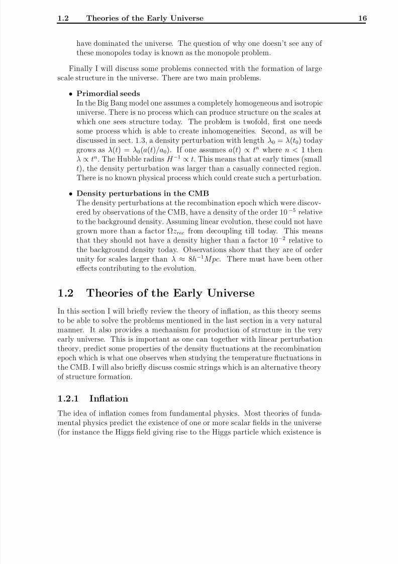
Figure 1.2: The potential of a scalar field
In Figure (1.2), I have sketched one possible potential for a scalar field Φ.One sees that for a temperature T higher than the critical temperature T c, thepotential had a minimum at Φ = 0. After the temperature dropped below T c,a deeper minimum arose at Φ = σ. From this point, the scalar field was notat its real minimum and the universe is said to have a false vacuum. Then thescalar field rolled or tunneled down to the real minimum (or real vacuum). Atthe end, the scalar field oscillated around the new minimum, interacting withmatter fields and creating particles. This is called the reheating period since theuniverse again got hot after it cooled significantly during the expansion period.

8/3/2019 Frode Kristian Hansen- Data Analysis of the Cosmic Microwave Background
http://slidepdf.com/reader/full/frode-kristian-hansen-data-analysis-of-the-cosmic-microwave-background 26/216
1.2 Theories of the Early Universe 18
It can be shown that in such a phase transition, the equation of state of theuniverse is p = −ρ. Looking at equation 1.4, one sees that the universe in thiscase has positive acceleration. Moreover, if the phase transition occur in sucha way so that the energy density of the universe is roughly constant for a shortperiod of time, then equation 1.4 says that a/a is constant. This means thata(t)
∝eAt. The expansion of the universe becomes exponential . A short period
with exponential expansion in the very early universe can solve most of the prob-lems in the standard Big Bang scenario.
If one assumes that the scale factor during a short period of inflation increasedby a factor of 1030, one can immediately see how the flatness problem is solved.By looking at equation (1.15), one can see that Ω is driven to 1 by such a largegrowth of the scale factor. So inflation actually predicts the universe to be very nearly flat. For this reason, one can set k = 0 in the Friedmann equations(Although k = 0 the term is so small compared to the other terms, that k iseffectively 0).
The horizon problem is also naturally solved in this scenario. By evaluatingthe integrals in equation (1.14) using a(t) ∝ eHt in the inflationary epoch, one seesthat a light ray could have been traveling much longer (in physical coordinates)from the beginning of the universe till recombination, than from recombinationand till today. In other words, the whole observable universe today was inside acasually connected region before inflation. This could explain the uniformity of the CMB temperature. The monopole problem is similarly solved. During theinflation, the number of monopoles per comoving volume element was constant,but the physical size of this volume element increased, so the physical density of monopoles decreased with a large factor. Estimates with inflation predicts at theorder of one monopole inside the current observable universe.
Finally inflation can solve the problem of the origin of structure in the uni-verse. Before and under inflation, quantum fluctuations in the scalar field Φ madesome regions of space to have a higher field value Φ + δΦ than the background.These regions had a size of the order of a Planck length before inflation. Duringinflation, the size of these regions (in physical coordinates) expanded with thescale factor. At the end of inflation, the size of these perturbation could havebeen big enough as to act as seeds for the large scale structure that the universeexhibits today. One important thing to notice here is that most theories predictthese quantum fluctuations to be Gaussian distributed. This means that inflation predicts Gaussian density perturbations in the early universe. The evolution of the perturbations from the end of inflation to the recombination era is linear sothe density fluctuations in that epoch should also be Gaussian. For this reasonchecking that the temperature fluctuations in the CMB are indeed Gaussian willbe an important test of inflation.
8/3/2019 Frode Kristian Hansen- Data Analysis of the Cosmic Microwave Background
http://slidepdf.com/reader/full/frode-kristian-hansen-data-analysis-of-the-cosmic-microwave-background 27/216
1.2 Theories of the Early Universe 19
Inflation also has a prediction for the density fluctuations. The predictionsays that the density fluctuations should be almost scale invariant , meaning thatthere should be a roughly equal number of fluctuations on all physical scales. Tounderstand this one needs to study how the fluctuations in the energy densitycan arise during inflation. Because of the presence of a horizon, there is confine-ment in space which due to the uncertainty principle leads to fluctuations in the
energy/momentum of the fields present. The size of these fluctuations will bedependent on the horizon size which is almost constant during inflation. Thismeans that the size of the fluctuations arising during inflation will be the sameduring the whole inflationary period. Inflation then expands these fluctuationsout of the causal horizon and they are frozen in. For this reason, the fluctuationson all scales will have a constant amplitude when they reenter the horizon at alater stage. This will be discussed further in section (1.3).
1.2.2 Cosmic Strings
As mentioned before, during phase transformations in the early universe, mag-netic monopoles should have been created. Magnetic monopoles are just onetype of the so called topological defects. In this section I will briefly mentionanother type, called cosmic strings. The theory of cosmic strings was competingwith inflation about being the main source of structure in the universe. Duringthe last years, this theory has been more or less ruled out, leaving inflation asthe main explanation for the origin of large scale structure. However the cosmicstrings could still have played a role, even if they didn’t give the main contri-bution to structure formation. After all, theories of fundamental physics predictthese phase transformations which give rise to cosmic strings to have taken place,
and for this reason cosmic strings should also have been formed.
To explain what a cosmic string is, I will use as an example a complex scalarfield Φ which for a temperature T higher than a critical temperature T c, has itsminimum potential energy at Φ = 0. At this temperature the Lagrangian andthe vacuum expectation value < Φ >= 0 are invariant under local U (1) transfor-mations Φ → Φeiα(x). At a temperature T < T c, the potential energy has a newminimum at |Φ| = σ. In this case, the U (1) symmetry is broken, as the vacuumexpectation value is now not invariant under the transformation Φ → Φeiα(x).The new vacuum expectation value < Φ >= σeiθ(x) can have a different phaseat different location (and will also necessarily have different phases, as different
points in space which are not casually connected cannot ’know’ what phase theother points have.) But if one starts at one point and go through a loop in a twodimensional plane and end up at the same point, the phase must change throughthis loop with an integer multiple of 2π. Say that one has such a loop with∆θ = 2π. If one shrinks this loop to a point, ∆θ can not change continuously

8/3/2019 Frode Kristian Hansen- Data Analysis of the Cosmic Microwave Background
http://slidepdf.com/reader/full/frode-kristian-hansen-data-analysis-of-the-cosmic-microwave-background 28/216
1.3 The Growth of Perturbations in the Early Universe 20
from ∆θ = 2π to ∆θ = 0. For this reason, there must be a point in the middlewhich doesn’t have a phase, namely the old minimum < Φ >= 0. So one endsup with a string in space having a false vacuum, that is the potential energy of the scalar field along this string is higher than that for the true vacuum (wherethe vacuum expectation value is at the minimum of the potential).
The cosmic string can act as gravitational attractors and seed structure for-mation. Cosmic strings lead to non-Gaussian density fluctuations and can in thisway be distinguished by the fluctuations created by inflation. Strings that formedbefore inflation probably got so diluted during inflation that there are hardly anyleft (this is what solved the monopole problem). If they formed after inflation,they could still be around and to some extend have contributed to structure for-mation in the early universe. If they are there, they should be visible in the CMBas non-Gaussian features.
1.3 The Growth of Perturbations in the Early
Universe
In this section I will review how density fluctuations which arose in the very earlyuniverse evolve. I will first discuss the linear regime (sect.1.3.1) where the densityfluctuations can be represented as ρ = ρ0+ρ1, where ρ0 is the background densityand ρ1 is a perturbation ρ1 ρ0. I will discuss how the fluctuations evolvedduring the radiation dominated era, in the matter dominated era and beyond therecombination epoch. In section 1.3.2 I will briefly discuss the evolution when thefluctuations became so large that the linear perturbation theory becomes invalid.Finally, the matter power spectrum which is used to quantify the fluctuations is
defined in section 1.3.3.
1.3.1 Linear Evolution
In the early universe, the density fluctuations where so small compared to thebackground density that the use of linear perturbation theory is justified. Twocases need to be distinguished. The perturbations which are significantly smallerthan the Hubble radius can be treated with Newtonian dynamics. The super-horizon size perturbations however, need a fully relativistic treatment.
I will start by the superhorizon sized perturbations. When the superhorizonperturbations are treated with the relativistic formalism, there is an additionalcomplication due to a gauge freedom . When doing perturbation theory, one workswith a uniform ‘background spacetime’ and a physical spacetime which is simi-lar to the background spacetime but with small pertubations added to it. The

8/3/2019 Frode Kristian Hansen- Data Analysis of the Cosmic Microwave Background
http://slidepdf.com/reader/full/frode-kristian-hansen-data-analysis-of-the-cosmic-microwave-background 29/216
1.3 The Growth of Perturbations in the Early Universe 21
gauge freedom which arises, is the freedom to choose the correspondence be-tween coordinated of points in the background spacetime and in the perturbedphysical spacetime. A gauge transformation is a change in this correspondence,keeping the coordinates of the background spacetime fixed (Bardeen 1980). Thetreatment of superhorizon sized perturbations is traditionally done in the syn-chronous gauge, but as this gauge has problems with coordinate singularities, the
Newtonian conformal gauge has been used in newer treatments. Some studies of perturbations growth have been using gauge invariant quantities. For a reviewof these different approaches, see (Ma and Bertschinger 1995). To avoid theseproblems, I will use some simple arguments instead of the complete relativisticformalism to estimate the growth of superhorizon sized perturbations. This givesthe same result as the relativistic approach.
Consider a flat (k = 0) universe with a uniform density ρ0 and Hubble constantH . The Friedmann equations give for this universe,
H
2
=
8πG
3 ρ0. (1.17)
In this universe, one has a super horizon sized area with a slightly different densityρ0 + ρ1. This part of the universe can be treated as a part of the universe whichis no longer flat (because of the difference in density) and therefore with k = 0.Inside this area one has,
H 2 +k
a2=
8πG
3(ρ0 + ρ1). (1.18)
These two equations together give for the size of the density fluctuations describedby δ = ρ1/ρ0
δ ≡ ρ1ρ0
∝ (ρ0a2)−1. (1.19)
This gives for matter and radiation dominated universes δ ∝ a and δ ∝ a2 re-spectively.
As the fluctuations grow, their sizes will at some point become smaller thanthe horizon at a given epoch. They enter the horizon at a time tenter. When thefluctuations have entered the horizon, one can use Newtonian physics to describetheir further evolution by using the equations of motions for an expanding perfectfluid. The Eulerian equations for a perfect fluid are given as,
∂ρ∂t
+ · (ρv) = 0, (1.20)
∂ v
∂t+ (v · )v +
1
ρ p + φ = 0, (1.21)
2φ = 4πGρ, (1.22)

8/3/2019 Frode Kristian Hansen- Data Analysis of the Cosmic Microwave Background
http://slidepdf.com/reader/full/frode-kristian-hansen-data-analysis-of-the-cosmic-microwave-background 30/216
1.3 The Growth of Perturbations in the Early Universe 22
where the expansion of the universe is not taken into account. This will beincluded later. Here ρ = ρ(r, t), p = p(r, t) and φ = φ(r) are the density, pressureand gravitational potential respectively at position r at time t. The fluid velocityis v = v(r, t). Now consider small perturbations of these quantities aroundthe background value. One can denote the background by subscript 0 and theperturbation by subscript 1. One can then use
= 0 + 1 (1.23)
in the Eulerian equations. Here can be ρ, p, v and φ. The resulting equationsfor the perturbations are
∂ρ1
∂t+ ρ0 · v1 = 0, (1.24)
∂ v1∂t
+v2sρ0
ρ1 + φ1 = 0, (1.25)
2φ1 = 4πGρ1. (1.26)
Here vs is the speed of sound
v2s ≡
∂p
∂ρ
adiabatic
=p1ρ1
, (1.27)
where the last equality comes about because of the assumption that there is nowspatial variations in the equations of state. Combining these equations one getsthe differential equation
∂ 2ρ1∂t2
− v2s2ρ1 = 4πGρoρ1. (1.28)
Solving for the density perturbation ρ1, one gets
ρ1(r, r) = Aρ0e−ik·r+iωt. (1.29)
Inserting this solution into the differential equation (equation 1.28) one finds thedispersion relation
ω2 = v2s k2 − 4πGρ0. (1.30)
Here k = |k|. From the dispersion relation (equation 1.30), one easily sees thatfor
k < kJ
, kJ
= 4πGρ0
v2s, (1.31)
one gets imaginary values for ω. The wavenumber kJ is called the Jeans wavenum-ber and determines whether ω is real or imaginary. In the case of an imagi-nary ω, one sees that the solution (equation 1.29) is exponentially growing withtime. In the other case, the perturbation is oscillating. So the Jeans wavelength
8/3/2019 Frode Kristian Hansen- Data Analysis of the Cosmic Microwave Background
http://slidepdf.com/reader/full/frode-kristian-hansen-data-analysis-of-the-cosmic-microwave-background 31/216
1.3 The Growth of Perturbations in the Early Universe 23
λJ = 2π/kJ is the limiting wavelength. Perturbations bigger than this will beexponentially growing and perturbations which are smaller will be oscillating.Physically one can understand this as the battle between gravitation and pres-sure. Gravitation is trying to make the perturbation bigger whereas pressure istrying to make it smaller by resisting contraction. When the size of the pertur-bation is bigger than the Jeans wavelength, the force of Gravity is big enough to
win over pressure.
To make this analysis cosmologically relevant, the expansion of the universehas to be taken into account. For an expanding universe, the zeroth order solutionto the fluid equations is
ρ0 = ρ0(t0)a−3, (1.32)
v0 = H r, (1.33)
φ0 =4πGρ0
3r. (1.34)
Perturbing around this solution,
ρ = ρ0(t0)a−3 + ρ1, (1.35)
v0 = H r + v1, (1.36)
φ0 =4πGρ0
3r + φ1, (1.37)
and solving the Eulerian equations after Fourier transforming one finds the dif-ferential equation
δk + 2H δk + v2s k2
a2 −4πGρ0 δk = 0. (1.38)
here δk is the Fourier transform of the perturbation δ = ρ1/ρ0,
δ(r, t) = (2π)−3V
δk(t)e−ik·r/a(t)d3r, (1.39)
where V is the volume of integration. As before, the sign of the factor before thelast term in equation (1.38) is determining whether one gets growing or oscillatingsolutions. The Jeans wavelength in the expanding universe is given by
kJ = 4πGρ0a2
v2s . (1.40)
If k kJ the perturbation is growing. In this case one can write equation (1.38)as
δ + 2H δ − 4πGρ0δ = 0, (1.41)

8/3/2019 Frode Kristian Hansen- Data Analysis of the Cosmic Microwave Background
http://slidepdf.com/reader/full/frode-kristian-hansen-data-analysis-of-the-cosmic-microwave-background 32/216
1.3 The Growth of Perturbations in the Early Universe 24
where the k subscript is dropped, as this is valid for both δ and δk. The exactsolution is dependent on the parameters of the universe. In a flat Ω = 1 uni-verse in the matter dominated era, H = 2
3t−1 and ρ0 = 16πG t−2. Trying with the
solution δ = tn inserted into equation (1.41), one finds that δ ∝ t2/3 is a grow-ing mode solution. Apparently the expansion of the universe prevents the fastexponential growth of perturbations in the non-expanding model described above.
To study the evolution in the radiation dominated era, one has to take intoconsideration that there are different types of particles present. In this case,the total mass density ρ0 is a sum over densities ρ j of each species j present.For a species i which is non-relativistic (this is what was assumed in the abovederivation), equation (1.41) can then be written
δ + 2H δ − 4πGρ0
j
jδ j = 0, (1.42)
where the sum over j is a sum over the non-relativistic species and j = ρ j/ρ0.Assuming that there are only two species, photons and the non-relativistic species
i, the equation can be written as ( j 1 as photons are dominating in theradiation dominated era),
δ +1
tδ = 0, (1.43)
with the solution δ ∝ ln t. This shows that in the radiation dominated era, theperturbations can hardly grow.
From the above analysis, it seems that a significant growth of perturbationswill be postponed to after t = teq. After matter-radiation equality, the perturba-tions could in principle have started growing, but only if there were perturbationspresent which were big enough to start growing. If one assumes a spherical den-sity perturbation of size λ, the mass of this perturbation is (assuming uniformdensity)
M =4π
3ρ
λ
2
3
. (1.44)
For this perturbation to start growing, its size λ must be bigger than the Jeanslength λJ , or stated differently, the mass of the perturbation M , must be biggerthan the Jeans mass M J , corresponding to the mass of a spherical perturbationwith length λJ . Assuming a model with two species, baryons and photons, itcan be shown that before recombination when the photons are coupled to thebaryons, the Jeans mass is bigger than the total mass inside the horizon. Hence,the perturbation cannot start growing as there are now perturbation within thehorizon being big enough to have a stable growing mode. After recombinationwhen the pressure is dominated by the hydrogen atoms, the Jeans mass becomesconsiderably smaller and perturbations can start growing.

8/3/2019 Frode Kristian Hansen- Data Analysis of the Cosmic Microwave Background
http://slidepdf.com/reader/full/frode-kristian-hansen-data-analysis-of-the-cosmic-microwave-background 33/216
1.3 The Growth of Perturbations in the Early Universe 25
From observations of the CMB, the density fluctuations δ in the recombina-tion epoch were of the order 10−5 and as mention in section (1.1.2), this is notbig enough for the perturbations to be able to grow to the current size today.From the analysis in this section, one can see a solution to this problem. If therewas a particle species present which does not couple to the photons, densityperturbations in this species could have started growing just after t = teq and
before recombination. The non-baryonic dark matter which existence has beenindicated by several observations (e.g. of rotation curves of galaxies), could besuch a species. As the species is not coupled to the photons, the evolution of density perturbations was independent of the photon pressure and could thereforhave started growing before recombination. The perturbations in this specieswould have grown between t = teq and t = trec. After recombination when thebaryonic matter perturbations started growing, the gravitational force from thedensity perturbations in the non-baryonic component would increase the speedof the growth of baryonic density perturbations.
1.3.2 Nonlinear Evolution
The linear perturbations theory for density fluctuations in the early universe canbe used when the density perturbations are small δ 1. At some point, asthe perturbations were growing, it had reached a density which was consider-ably higher than the background density of the universe and linear perturbationstheory breaks down. In the nonlinear regime, the evolution of the density per-turbations was very complex. Here I will just briefly consider the properties of this nonlinear evolution.
The model used in the beginning of sect.(1.3.1), describing a flat universe(k = 0) containing a region with slightly different density can be used here. Inthat model, the flat universe has a scale factor a(t) and the part of the universecontaining an overdense region has a scale factor a(t). As I now describe a regionwhich has a higher density than the surrounding flat universe, this region willexpand and eventually collapse as the density is higher than the critical one. Theevolution of the scale factor a in this closed ’universe’ with Hubble constant H
and density parameter Ω can be represented by a parameterized set of equations,
a
ai= (1 − cos θ)
Ωi
Ωi − 1
, (1.45)
H it = (θ − sin θ) Ωi
2(Ωi − 1)3/2
. (1.46)
Here the index i describes the parameters at some fixed time ti. Knowing theparameters Ω
i, ai and H i one can use the equations to find the expansion param-eter a at any given time. The density fluctuation will have reached its maximum

8/3/2019 Frode Kristian Hansen- Data Analysis of the Cosmic Microwave Background
http://slidepdf.com/reader/full/frode-kristian-hansen-data-analysis-of-the-cosmic-microwave-background 34/216
1.3 The Growth of Perturbations in the Early Universe 26
expansion when θ = π, giving
amax
ai=
Ωi
Ωi − 1, (1.47)
H itmax =π
2
Ωi
(Ωi
−1)3/2
≈ π
2
amax
ai
3/2
, (1.48)
with a density
ρmax = ρi
ai
amax
3
=3π
32Gt2max(ρC )i
. (1.49)
Taking the time ti, so early that the density was the same as the backgrounddensity ρi = ρi = (ρc)i = (ρc)i. Then the density at the maximum expansion of the perturbation is
ρmax =3π
32Gt2max
, (1.50)
giving
δmax = ρmax
ρmax− 1 = 9π2
16− 1 ≈ 4.55. (1.51)
At the maximum expansion, the kinetic energy of the overdense region isE k = 0, whereas the gravitational energy E g = C/rmax where C is a constant.After the maximum expansion, the region starts collapsing and collapses untilE k = −E g/2. This is called virialisation and when the overdense region has viri-alised it has a gravitational energy of E g = C/rvir . Equalizing the total energyE t = E k + E g at maximum and after virialisation one finds that rvir = rmax/2,meaning that the density has increased by a factor of 8 from maximum expansionto virialisation.
1.3.3 The Matter Power Spectrum
In the previous sections I have described how the structures in the universe mighthave arisen in the very early universe and how they should have evolved to thepresent era. The next step is to find some way of characterising this structureso that the theoretical predictions can be compared to observations. The densityfluctuations δ(x) at a position x in the universe at some early time t, is a random
variable. I will in the following be assuming that this is a Gaussian distributedrandom variable with ensemble averaged mean value < δ >= 0. This is the pre-diction of inflation. As will be discussed, parts of the formalism is also valid if these assumptions do not hold.

8/3/2019 Frode Kristian Hansen- Data Analysis of the Cosmic Microwave Background
http://slidepdf.com/reader/full/frode-kristian-hansen-data-analysis-of-the-cosmic-microwave-background 35/216
1.3 The Growth of Perturbations in the Early Universe 27
The first thing I will define is the autocorrelation function describing theensemble average correlation between δ(x) and the fluctuation at some otherpoint δ(x + r) displaced by a vector r. This is simply defined as,
ξ(r) =< δ(x)δ(x + r) > . (1.52)
This can easily be Fourier transformed to give,
ξ(r) = (2π)−3V −1
|δk|2e−ik·rd3k, (1.53)
|δk|2 = V
ξ(r)eik·rd3r, (1.54)
where δk is the Fourier transformed density fluctuation given by equation (1.39)and V is the integration volume. The power spectrum of matter density fluctua-tions is defined in this way as P (k) = |δk|2. Since the density fluctuations evolvein time due to gravitational interactions, so does the power spectrum. The initial power spectrum is often assumed to be a power law of the form P (k) = AV kn,
where n is the spectral index and A is the amplitude.
Since < δ > is zero, one could calculate what the rms fluctuation σ2 =< δ2 >is. Some algebra gives,
σ2 =1
2π2
∞0
P (k)k2dk. (1.55)
This is the integral of the power spectrum over k-space. Unfortunately the quan-tity σ2 does not say anything about the relative contribution from different scalesk. For this reason, it is convenient to define the mass variance for a given lengthscale R. Defining a sphere of radius R, the mean mass < M > found inside sucha sphere is
< M >=< ρ > V = 4π3
< ρ > R3. (1.56)
This leads to the definition of the mass variance for a certain mass scale M ,
σ2M =
(δM )2
< M >2=
< (M − < M >)2 >
< M >2. (1.57)
For the power law initial power spectrum, the initial mass variance for a massscale M can be shown to scale as
σM ∝ k3/2δk ∝ k3α ∝ M −α, (1.58)
where α = (3 + n)/6 for the power law power spectrum.
As discussed in the section on inflation (sect.1.2.1), the perturbations pro-duced in inflation are supposed to have the same amplitude at all scales. Theyare supposed to be scale invariant . In this case, this refers to the perturbations
8/3/2019 Frode Kristian Hansen- Data Analysis of the Cosmic Microwave Background
http://slidepdf.com/reader/full/frode-kristian-hansen-data-analysis-of-the-cosmic-microwave-background 36/216
1.4 The Recombination Era and the CMB 28
produced in the gravitational potential φ. These perturbations can be estimatedusing the shape of the Newtonian gravitational potential
δφ ∝ GδM
M ∝ δM
M
M
R∝ σM M 2/3. (1.59)
Looking at equation (1.58), one sees that for the initial power spectrum of per-turbations to be scale invariant, α must be 2/3 and therefore the spectral indexn must be one.
The evolution of the power spectrum with time can be found by studyingthe evolution of δ with time. In linear perturbation theory, one can describe theevolution of δk(t) as
δk(t) = T k(t, ti)δk(ti). (1.60)
Here T k(t, ti) is the transfer function which describes the evolution of the k modeof density perturbations from some initial time ti to time t. This gives for thepower spectrum
P (k, t) = |T k(t, ti)|2P (k, ti). (1.61)
In the linear regime, one can find the transfer functions, using the linear theoryof the evolution of density perturbations outlined above. In the nonlinear regime,finding the transfer function is non trivial as it is not quite known which physicalprocesses were dominant during the epoch of nonlinear growth of perturbations.
Finally, when using the linear theory one finds that the power spectrum of fluctuations at the time when the fluctuation with wavenumber k entered thehorizon is given by
P (k, tenter) ∝ kn−4, (1.62)
so that σM (tenter) ∝ kn−1, (1.63)
which for the Harrison-Zeldovich spectrum is independent of k. This means thatwhen n = 1, all fluctuations entered the horizon with the same amplitude.
1.4 The Recombination Era and the CMB
In this section I will discuss how the primary anisotropies in the CMB arose(sect.1.4.1). I will describe how the linearized Einstein equations for the densityperturbations can be used together with the the Boltzmann equation to predict
the anisotropies at the last scattering surface. Then in section 1.4.2 I will definethe CMB power spectrum and describe how it varies with some of the cosmologicalparameters. The small scale secondary anisotropies which arose when the CMBphotons passed through the reionized part of the universe will be briefly describedin section 1.4.3.

8/3/2019 Frode Kristian Hansen- Data Analysis of the Cosmic Microwave Background
http://slidepdf.com/reader/full/frode-kristian-hansen-data-analysis-of-the-cosmic-microwave-background 37/216
1.4 The Recombination Era and the CMB 29
1.4.1 The Origin of the CMB Anisotropies
To predict the shape of the temperature fluctuations ∆T /T observed in the CMB,one has to apply the Boltzmann equation describing the evolution of the photondistribution function in a photon-baryon gas with Compton scattering. The lineardensity perturbations will now be described using the gauge invariant potentials
Ψ and Φ described in (Bardeen 1980). These are related to the total densityperturbations δ and the anisotropic stress Π by
k2Φ = 4πGρ0
a
a0
2δk, (1.64)
Φ + Ψ = −8πGp
k2
a
a0
2Π. (1.65)
Here (and in the rest of the section), δk, Φ, Ψ and Π denote the Fourier trans-forms of the quantities δ, Φ, Ψ and Π respectively. The scale factor is as before a,the pressure is p. In a completely matter dominated universe where the pressure
p is unimportant, one sees that the two potentials are related by Ψ = −Φ.
The temperature anisotropy at position x in space at conformal time η = dt(a0/a) in the direction n will now be denoted ∆(x, n, η), and its Fourier
transform ∆k(µ, η) where k = |k| and µ = k · n/k. The Legendre expansion isgiven by,
∆k(µ, η) =
(−i)∆k(η)P (µ), (1.66)
where P (µ) is the Legendre Polynomial of order . Using these definitions, theBoltzmann equation for the temperature anisotropies becomes
∆k(µ, η)+ikµ(∆k(µ, η)+Ψ) =
−Φ+τ (η)[∆k0(η)
−∆k(µ, η)
−
1
10
∆k2(η)P 2(µ)
−iµV k(η)].
(1.67)Here a dot represents the derivative with respect to conformal time, V k is theFourier transform of the baryon velocity and τ = xeneσT a/a0 is the differentialoptical depth to Thompson scattering. The ionization fraction is given by xe, theelectron density by ne and the Thompson cross section by σT .
The evolution of the linear density perturbations in baryons δb and photonsδγ is given again by the continuity and Euler equations
(δb)k = −k(V k − ∆k1) +3
4(δγ )k (1.68)
V k = − aa
V k + kΨ + τ (∆k1 − V k)R
. (1.69)
Here R = 3ρb/(4ργ ). The universe is now supposed to consist of 3 species, thephotons, the baryons and the dark matter. The density fluctuations in the cou-pled baryon-photon fluid is described by the Boltzmann equation (1.67) and the
8/3/2019 Frode Kristian Hansen- Data Analysis of the Cosmic Microwave Background
http://slidepdf.com/reader/full/frode-kristian-hansen-data-analysis-of-the-cosmic-microwave-background 38/216
1.4 The Recombination Era and the CMB 30
Euler equations (1.68, 1.69). The dark matter is not coupled to any of thesespecies and only shows up through its influence on the gravitational potentials Ψand Φ.
Before recombination the photons were continuously scattered on the elec-trons. In such a case the photon distribution is isotropic in the electron rest
frame, so the dipole ∆k1 is only caused by the movement of the baryons, ∆k1 = V k.Inserting this into equation (1.68) one gets ( δb)k = 3/4(δγ )k, which is the equa-tion for for adiabatic evolution of the density fluctuations. This also gives that∆k = 0 for ≥ 2. This is called the tight coupling limit .
Close to the tight coupling limit one can use the the tight coupling approxima-tion . In this approximation equations (1.67), (1.68) and (1.69) can be expandedto first oder in the Compton scattering time τ −1. This gives the resulting differ-ential equation
∆k0 +a
a
R
1 + R∆k0 + k2c2s∆k0 = F (η), (1.70)
where F (η) is a term containing the gravitational potentials and cs is the soundspeed
cs =1
3
1
1 + R. (1.71)
This is the equation of a forced damped oscillator. The gravitational attraction of the over density regions pull the matter into this region, but the photon pressureresists the contraction, giving acoustic oscillations in the photon-baryon fluid.
The solution to equation (1.70), can be written as
∆k0(η) = a cos krs(η) + b sin krs(η) + c(F (η)), (1.72)
where the hat denotes that this is the solution in the thight coupling approxi-mation. The dipole goes as k∆k1 = −3(∆k0 + Φ) which means that it oscillateswith an angle π/2 out of phase with the monopole. Here rs is the sound horizon,given as
rs(η) = η
0csdη. (1.73)
Clearly, the amplitude of the dipole will be damped by a factor rs ∝ (1 + R)−1/2
with respect to the amplitude of the monopole.
In equation (1.72), the cos-term comes from adiabatic perturbations and the
sin-term from isocurvature perturbations. Adiabatic fluctuations are perturba-tions for which the entropy is constant causing the relation between the baryonand photon perturbation to δb = 3/4δγ . These kind of fluctuations are predictedby inflation. The isocurvature perturbations are perturbations in the entropy.For these perturbations which are expected by cosmic string models, δb = −δγ

8/3/2019 Frode Kristian Hansen- Data Analysis of the Cosmic Microwave Background
http://slidepdf.com/reader/full/frode-kristian-hansen-data-analysis-of-the-cosmic-microwave-background 39/216
1.4 The Recombination Era and the CMB 31
so that the total energy density is constant. Recent observations indicate thatadiabatic perturbations are dominant so that b ≈ 0 in the equation. For thisreason I will mainly discuss adiabatic perturbations in this thesis.
One sees that different k modes oscillate with a different frequency. At recom-bination η = ηrec, the monopole for some scales k is at its maximum or minimum
of the oscillations and will show up as peaks in the CMB temperature anisotropypower spectrum. For some other scales the monopole will be zero, and the CMBtemperature power spectrum has a trough, which is not zero due to the dipole(which has its maximum/minimum here due to the π/2 phase shift). The peaksand troughs in the temperature power spectrum resulting from these oscillationswill be described in more detail in section (1.4.2).
When recombination started, the mean free path of the photons became longeras there were less and less electrons present on which they could scatter. Thephotons were able to diffuse through the baryons and in this way the tempera-ture anisotropies at small scales were getting smaller. This is called Silk damping(Silk 1968). Another result of the increasing diffusion length, is that the CMBphotons that one can observe did not last scatter at the same time. The last scat-tering surface has a finite width and the photons come from different depths inthe surface where the oscillations in the monopole ∆k0 had different phases. Thishas the similar effect of smearing out the temperature anisotropies on small scales.
When scattering became less frequent the tight coupling limit breaks downand the equations (1.67), (1.68) and (1.69) have to be expanded to second oderin the Compton scattering time τ −1. The solution to this set of equations can bewritten as
(∆k0 + Ψ) = (∆k0 + Ψ)e−(k/k
D(η))2
, (1.74)where kD(η) is dependent on the diffusion length of the photons at time η. Thisexponential damping of small scales is caused by the above mentioned effects of photon diffusion and finite width of the last scattering surface.
To find the CMB temperature anisotropies today, the multipoles ≥ 2 of ∆k
have to be found. One can get these by solving the boltzmann equation (1.67),ignoring the quadrupole which disappears in the tight coupling limit and make amultipole expansion of the solution. The result is
∆k
(η0)
≈(∆
k0+ Ψ)(η
rec)(2 + 1) j
(k∆η
rec) (1.75)
+∆k1(ηrec)[j−1(k∆ηrec) − ( + 1) j+1(k∆ηrec)]
+(2 + 1) η0
ηrec(Ψ − Φ) j(k∆η)dη,
where j(x) is the Bessel function, ∆η = η0 − η and ∆ηrec = η0 − ηrec. The Silk

8/3/2019 Frode Kristian Hansen- Data Analysis of the Cosmic Microwave Background
http://slidepdf.com/reader/full/frode-kristian-hansen-data-analysis-of-the-cosmic-microwave-background 40/216
1.4 The Recombination Era and the CMB 32
damping and the damping due to finite with of the last scattering surface areincluded by
(∆k0 + Ψ)(ηrec) = (∆k0 + Ψ)(ηrec)D(k) ∆k1(ηrec) = ∆k1(ηrec)D(k), (1.76)
where
D(k) = η0
0 τ (η)e−τ (η,η0)
e−(k/kD(η))2
dη. (1.77)
One can see from equation (1.75) that the anisotropies in the CMB havethree main contributions. The first term in the equation is called the ordinary Sachs-Wolf effect (Sachs and Wolfe 1967). This is the sum of the monopole tem-perature differences on the last scattering surface and the gravitational potentialΨ. The gravitational potential accounts for the redshift of the photons as theyclimbed out of the potential wells of the density inhomogenieties at the last scat-tering surface. The second term in equation (1.75) is due to a Doppler shift.
Because of the acoustic oscillations before and at recombination, the baryonswere moving. When the photons were last scattered on these moving electrons,they experienced a Doppler shift. Finally, the last main contributor to the CMBanisotropy is the integrated Sachs-Wolf effect . This effect arose after the photonslast scattered. This is due to a possible time change in the gravitational potentialafter the recombination epoch. This term becomes important if matter-radiationequality occurred close to recombination, or if the universe has got Λ-dominatedafter recombination.
Clearly, these three terms are dependent on cosmological parameters. If theamount of dark matter and baryons are changed, the size of the density pertur-
bations and the gravitational potentials are also changed. This clearly results inchanges of the CMB anisotropies. The speed of expansion of the universe mea-sured by the Hubble constant, is of course also important in these calculations.As are the initial perturbations power spectrum produced by (possibly) inflation.In the next section, I will define the CMB temperature power spectrum of fluc-tuations and outline how it is dependent on some of these parameters. Equation(1.75) shows how important the CMB power spectrum can be for measuring thecosmological parameters.
1.4.2 The CMB Power Spectrum
I start by defining the am which are the coefficients of a spherical harmonicexpansion of the temperature fluctuations ∆T /T (θ, φ) on the sky,
am =
S dnT (n)Y m(n), (1.78)

8/3/2019 Frode Kristian Hansen- Data Analysis of the Cosmic Microwave Background
http://slidepdf.com/reader/full/frode-kristian-hansen-data-analysis-of-the-cosmic-microwave-background 41/216
1.4 The Recombination Era and the CMB 33
where T (n) is the fluctuation ∆T /T in the position n and Y m(n) are the sphericalharmonic functions. The integration is performed over the full sky denoted byS . If the initial density perturbations in the universe are Gaussian as predictedby most inflationary theories, so are the am. The angular power spectrum of theCMB is defined as,
C =
m=−
amam
2 + 1 , (1.79)
where is the multipole. Small -values represent large angular scales and high-values represent small angular scales. The relation between an -value and anangular scale ∆θ on the sky can be written as ∆θ ≈ 180/.
If the am are Gaussian distributed, the power spectrum C contain all theinformation contained in the CMB. Assuming isotropy of the universe, one hasthat < T (n)T (n) >= C (∆) where ∆ = n · n. This gives that the am areuncorrelated < amam >= δδmm < C >. One sees from equation (1.79)that for a given coefficient C , there are 2 + 1 independent statistical samples
of the average value for < C >. This means that for the higher multipoles, thestatistics is better and C for a given sky will be closer to the ensemble average< C >. The smaller multipoles has lower statistics and therefore suffer from theproblem of cosmic variance.
The angular power spectrum can be determined from the power spectrum ink-space derived in the last section, by
C =2V
π(2 + 1)2
k2|∆k(η0)|2, (1.80)
where V is an arbitrary normalisation constant.The Sachs-Wolfe effect is the dominant effect on large scales. I will now
estimate how the power spectrum C depends on from the Sahcs-Wolfe effect.At recombination, one can approximately set
∆k0(ηrec) ≈ −2
3Ψ(ηrec) ≈ −2
3Ψ(η0). (1.81)
Here it is assumed that the pressure is zero at recombination and that the po-tential has not changed from the last scattering surface and until today. So, onlylooking at the Sachs-Wolfe effect one gets from equation (1.75)
∆k(η0) ∝ Ψ(ηrec)(2 + 1) j(kx), (1.82)
where x = ∆ηrec. Using equation (1.80), one finds
C ∝
k2|Ψ(η0)|2 j2 (kx)dk. (1.83)
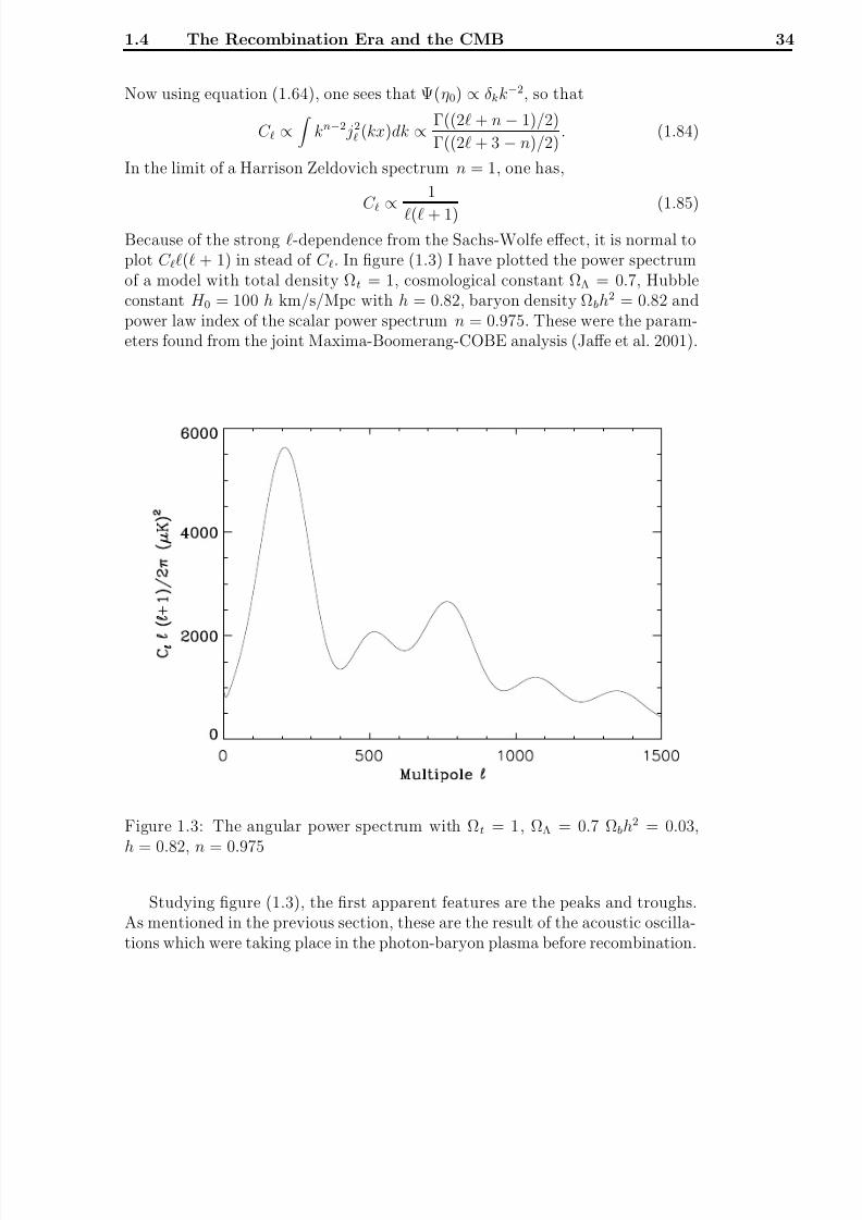
8/3/2019 Frode Kristian Hansen- Data Analysis of the Cosmic Microwave Background
http://slidepdf.com/reader/full/frode-kristian-hansen-data-analysis-of-the-cosmic-microwave-background 42/216
1.4 The Recombination Era and the CMB 34
Now using equation (1.64), one sees that Ψ(η0) ∝ δkk−2, so that
C ∝
kn−2 j2 (kx)dk ∝ Γ((2 + n − 1)/2)
Γ((2 + 3 − n)/2). (1.84)
In the limit of a Harrison Zeldovich spectrum n = 1, one has,
C ∝
1
( + 1)(1.85)
Because of the strong -dependence from the Sachs-Wolfe effect, it is normal toplot C ( + 1) in stead of C . In figure (1.3) I have plotted the power spectrumof a model with total density Ωt = 1, cosmological constant ΩΛ = 0.7, Hubbleconstant H 0 = 100 h km/s/Mpc with h = 0.82, baryon density Ωbh2 = 0.82 andpower law index of the scalar power spectrum n = 0.975. These were the param-eters found from the joint Maxima-Boomerang-COBE analysis (Jaffe et al. 2001).
Figure 1.3: The angular power spectrum with Ωt = 1, ΩΛ = 0.7 Ωbh2 = 0.03,
h = 0.82, n = 0.975
Studying figure (1.3), the first apparent features are the peaks and troughs.As mentioned in the previous section, these are the result of the acoustic oscilla-tions which were taking place in the photon-baryon plasma before recombination.

8/3/2019 Frode Kristian Hansen- Data Analysis of the Cosmic Microwave Background
http://slidepdf.com/reader/full/frode-kristian-hansen-data-analysis-of-the-cosmic-microwave-background 43/216
1.4 The Recombination Era and the CMB 35
The peaks are resulting from the k modes of the monopole ∆k0(ηrec) which wereat their minimum/maximum at recombination. The troughs occur where themonopole was 0. These are filled in by the dipole which was oscillating π/2 outof phase and for this reason had its minima/maxima in the troughs. The dipolehowever had a lower amplitude.
Assuming adiabatic fluctuations, equation (1.72) tells us that one can expectthe first peak at k = π/rs, which is the scale of the sound horizon at last scatter-ing. In a flat universe, the sound horizon at the last scattering surface is expectedto have an angular size of about one degree on the sky. This means that for flatuniverses with adiabatic fluctuations one should expect to see the first peak at aposition of ≈ 200. This fits very well with the current data. When the universehas less matter, the universe is open and the geometry of the universe is hyper-bolic. In this case the same physical scales at recombination corresponds to asmaller angle on the CMB sky than in the flat universe. So for an open universe,the first peak was expected to be found at higher values. Also in the case of isocurvature perturbations, the peak should have been at higher since in thiscase the wave number for the first peak should be k = π/(2rs) corresponding tolarger scales. One already sees here how the CMB power spectrum can be usedto measure values and properties of the universe.

8/3/2019 Frode Kristian Hansen- Data Analysis of the Cosmic Microwave Background
http://slidepdf.com/reader/full/frode-kristian-hansen-data-analysis-of-the-cosmic-microwave-background 44/216
1.4 The Recombination Era and the CMB 36
Figure 1.4: The solid line shows the angular power spectrum with Ωt = 1.0,ΩΛ = 0.7 Ωbh2 = 0.03, h = 0.82, n = 0.975. The other curves are the powerspectra for lower total density Ω = Ωt. The ratios between Ωb, Ωc and ΩLambdaare kept constant.
In figure (1.4) one can see how the peaks are moving to larger scales as thetotal density is decreasing. I have chosen the same model as in figure (1.3), butvaried the total density Ω from 0.3 to 1.0 by keeping the ratios of baryon density,dark matter density and vacuum energy density constant.
Another effect is the change of heights of the peaks as the baryon fraction ischanged. As described above, the peaks of the power spectrum come from themaximum and minimum of the acoustic oscillations. The oscillations are drivenby the gravitational force contracting the density perturbations and the photonpressure resisting this contraction. Every second peak, starting with the first one
are coming from the contraction phase. The stronger the contraction, the higherthese peaks should be. The other peaks come from the rarefaction phase.

8/3/2019 Frode Kristian Hansen- Data Analysis of the Cosmic Microwave Background
http://slidepdf.com/reader/full/frode-kristian-hansen-data-analysis-of-the-cosmic-microwave-background 45/216
1.4 The Recombination Era and the CMB 37
Figure 1.5: The solid line shows the angular power spectrum with Ωt = 1.0,ΩΛ = 0.7 Ωbh2 = 0.03, h = 0.82, n = 0.975. The other curves are the powerspectra for different baryon densities Ωb. The sum of baryons and dark matter iskept constant, Ωb + Ωc = 0.3.
When the baryon content of the universe is higher, the mean free path of the photon and the photon pressure decrease. This means that the contractionswill have a higher amplitude and the rarefactions a smaller amplitude. In otherwords, raising the baryon fraction should increase the hight of the odd numberedpeaks in the angular power spectrum. Similarly the even numbered peaks shouldget lower. This is clearly seen in figure (1.5). In the figure I have again usedthe model in figure (1.3), but this time varied the baryon density to dark matterdensity ratio, keeping the total density Ωb + Ωc = 0.3 and ΩΛ = 0.7.
From these discussion it should be apparent that the angular power spectrum
of the CMB is an important source of the cosmological parameters. By estimat-ing the power spectrum from measurements of the CMB one should be able tomeasure the cosmological parameters with a very high precision. Some othercosmological parameters that one can measure from the power spectrum includethe Hubble parameter h, the dark matter content Ωc, the power law index of the
8/3/2019 Frode Kristian Hansen- Data Analysis of the Cosmic Microwave Background
http://slidepdf.com/reader/full/frode-kristian-hansen-data-analysis-of-the-cosmic-microwave-background 46/216
1.4 The Recombination Era and the CMB 38
power spectrum of scalar and tensor perturbations (tensor perturbations will bediscussed in the next section) ns and nt, the redshift of reionization zreion, thenumber of neutrino degrees of freedom at decoupling N ν , the normalisation of the matter power spectrum Q and the ration of tensor to scalar perturbationsQ2
T /Q2S (Jungman, Kamionkowski, Kosowsky, and Spergel 1996).
1.4.3 Reionization and Secondary Anisotropies
After recombination, the universe was reionized at some redshift zreion, whichis still unknown. For this reason CMB photons might have been scattered onelectrons after recombination. This scattering might have influenced the CMBpower spectrum. If reionization happened early (zreion > 30) this rescatter-ing might have erased the peaks in the CMB power spectrum and thereby alsoimportant information about the universe. As discussed above, the present ob-servations have revealed a peak structure in the power spectrum indicating thatreionization happened in an epoch which was so late that the scattering afterrecombination did not have a significant influence on the CMB on the scaleswhere most of the cosmological information is stored. They could however be thedominant contribution to the power spectrum on smaller scales ( > 1000).
Here I list some effects that reionization might have on the power spectrum:
1. Vishniac effect: During the epoch of galaxy formation, there were hugemoving gas masses on which the CMB photons were scattered. The Doppleshift from the scattering on these moving electrons should have influencedthe angular power spectrum on smaller scales (Ostriker and Vishniac 1986;
Vishniac 1987; Persi, Spergel, Cen, and Ostriker 1995). The strength of this effect and the scales at which it is important is dependent on thereionization history of the universe.
2. Thermal Sunyaev Zeldovich effect: When CMB photons passed through hotelectron gas in clusters of galaxies and superclusters, their frequencies werechanged due to Compton scattering (Zeldovich and Sunyaev 1969). The hotelectrons in the clusters transferred energy to the photons resulting in anupscattering of the photon frequency. For this reason the clusters resultedin a temperature decrement at lower frequencies and increment at higherfrequencies. This effect has been observed and has been used to measure
the Hubble constant (see e.g. (Myers, Baker, Readhead, and Leitch 1997)).The SZ effect is only expected to give significant contributions to the CMBpower spectrum on smaller scales (Persi, Spergel, Cen, and Ostriker 1995).
3. Kinetic Sunyaev Zeldovich effect: Because of the peculiar velocities of theclusters of galaxies, there will be an additional Doppler shift of the CMB

8/3/2019 Frode Kristian Hansen- Data Analysis of the Cosmic Microwave Background
http://slidepdf.com/reader/full/frode-kristian-hansen-data-analysis-of-the-cosmic-microwave-background 47/216
1.4 The Recombination Era and the CMB 39
photons scattered on the electron gas in clusters. This is called the kine-matic SZ effect and is about an order of magnitude smaller than the thermaleffect. The two effects can be distinguished because of their different spec-tral signatures. The kinetic effect can in principle be used to measure thepeculiar velocities of clusters (Sunyaev and Zeldovich 1980).
There are also other small scale effects caused by gravitation. One of themis associated with the integrated Sachs-Wolfe effect for the time varying gravi-tational potentials from nonlinear evolution of density perturbation. The move-ments of the gas in the density fluctuations in the epoch of nonlinear growth wasmaking the gravitational potential time varying and thereby causing a gravita-tional frequency shift of the CMB photons passing through the perturbation (seeequation (1.75)). This is called the Rees-Sciama effect (Rees and Sciama 1968)and is contributing (being of the order of magnitude of the primordial pertur-bations) to the power spectrum on very small scales (typically -values of a fewthousand).
Finally gravitational lensing of the CMB by foreground galaxies and galacticclusters might also have influenced the power spectrum. This effect tends tosmooth out the peak structure in the power spectrum (Seljak 1996).
1.4.4 Polarisation of the CMB and Tensor Perturbations
Some of the cosmological parameters have similar effects on the power spectrum.For this reason several combinations of cosmological parameters may give thesame power spectrum. This degeneracy of parameters may be broken by lookingat the polarisation of the CMB. Since Thompson scattering produce linear pho-ton polarisation , the CMB photons are expected to be linearly polarised.
Polarisation of photons are usually characterized by the Stokes parameters I ,Q, U and V . Here I is the total intensity, Q and U describe linear polarisationand V circular polarisation. Since Thompson scattering is unable to produce cir-cular polarisation, V is excpected to be zero in the CMB and will for this reasonnot be treated further here.
I will now define the Stokes parameters following (Chandrasekhar 1960). TheQ and U Stokes parameters can be defined by the components of the electric vec-tor of electromagnetic radiation decomposed in two directions x and y which aremutually perpendicular and also perpendicular to the direction of propagation of
the radiation. For a plane electromagnetic wave, the components can be writtenas
E x = E x0 cos(ωt − δx), (1.86)
E y = E y0 cos(ωt − δy), (1.87)

8/3/2019 Frode Kristian Hansen- Data Analysis of the Cosmic Microwave Background
http://slidepdf.com/reader/full/frode-kristian-hansen-data-analysis-of-the-cosmic-microwave-background 48/216
1.4 The Recombination Era and the CMB 40
where E x0 and E y0 are the wave amplitudes and δx and δy are phases factors.One can then define intensity and the Stokes parameters as
I = E 2x0 + E 2y0, (1.88)
Q = E 2x0 − E 2y0, (1.89)
U = E x0E y0 cos(δx
−δy). (1.90)
As with the CMB temperature, the CMB polarisation will also have fluctua-tions which arose from the acoustic oscillation at the last scattering surface. It ispractical to make a spherical harmonic expansion of the CMB polarisation in thesame way as for the CMB temperature and describe the fluctuations in terms of polarisation power spectra. There are two approaches to this (Zaldarriaga andSeljak 1997; Kamionkowski, Kosowsky, and Stebbins 1997). In this thesis I willfollow (Zaldarriaga and Seljak 1997).
As for the temperature anisotropies, the fluctuations in Q and U can be
expanded in spherical harmonic coefficients am. For polarisation one has to usetensor harmonics 2Y m(n) and −2Y m(n) instead of normal scalar harmonicsY m(n). These tensor harmonics are described in appendix B. The coefficientscan be defined as (from now on Q(n) and U (n) are taken to be ∆Q/Q and ∆U/U to simplify notation.)
(Q + iU )(n) =m
a2,m 2Y m(n), (1.91)
(Q − iU )(n) =m
a−2,m −2Y m(n). (1.92)
The inverse relations are
a2,m =
dn 2Y ∗m(n)(Q + iU )(n), (1.93)
a−2,m =
dn −2Y ∗m(n)(Q − iU )(n). (1.94)
These spherical harmonic coefficients can be redefined in terms of their linearcombinations
aE,m = −(a2,m + a−2,m)/2, (1.95)
aB,m = i(a2,m − a−2,m)/2. (1.96)
The indices E and B only reflects the fact that these two coefficients have someproperties similar to the electric and magnetic fields. Using these coefficients,one can finally define the three power spectra of polarisation
C E =1
2 + 1
m
< a∗E,maE,m >, (1.97)
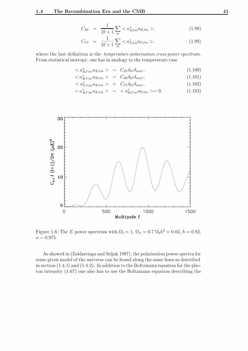
8/3/2019 Frode Kristian Hansen- Data Analysis of the Cosmic Microwave Background
http://slidepdf.com/reader/full/frode-kristian-hansen-data-analysis-of-the-cosmic-microwave-background 49/216
1.4 The Recombination Era and the CMB 41
C B =1
2 + 1
m
< a∗B,maB,m >, (1.98)
C C =1
2 + 1
m
< a∗T,maE,m >, (1.99)
where the last definition is the temperature-polarisation cross power spectrum .
From statistical isotropy, one has in analogy to the temperature case
< a∗E,maE,m > = C Eδδmm , (1.100)
< a∗B,maB,m > = C Bδδmm , (1.101)
< a∗T,maE,m > = C C δδmm , (1.102)
< a∗B,maE,m > = < a∗B,maT,m >= 0. (1.103)
Figure 1.6: The E power spectrum with Ωt = 1, ΩΛ = 0.7 Ωbh2 = 0.03, h = 0.82,n = 0.975.
As showed in (Zaldarriaga and Seljak 1997), the polarisation power spectra forsome given model of the universe can be found along the same lines as describedin section (1.4.1) and (1.4.2). In addition to the Boltzmann equation for the pho-ton intensity (1.67) one also has to use the Boltzmann equation describing the
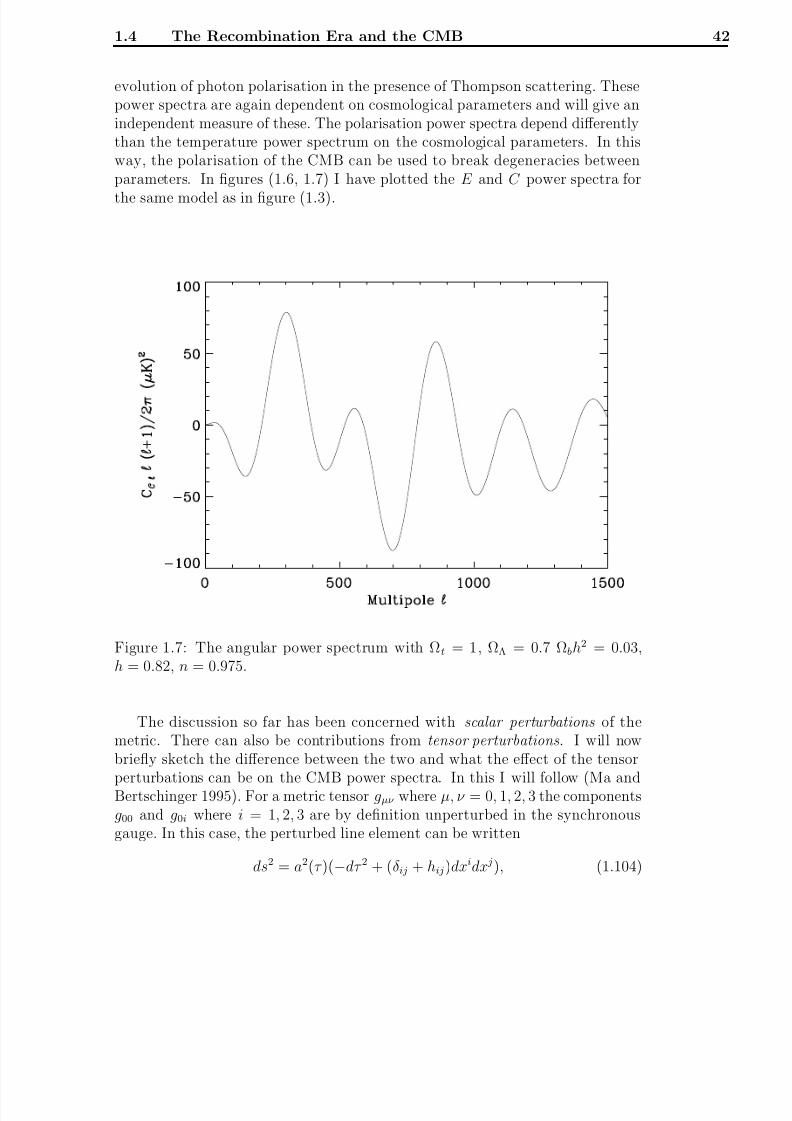
8/3/2019 Frode Kristian Hansen- Data Analysis of the Cosmic Microwave Background
http://slidepdf.com/reader/full/frode-kristian-hansen-data-analysis-of-the-cosmic-microwave-background 50/216
1.4 The Recombination Era and the CMB 42
evolution of photon polarisation in the presence of Thompson scattering. Thesepower spectra are again dependent on cosmological parameters and will give anindependent measure of these. The polarisation power spectra depend differentlythan the temperature power spectrum on the cosmological parameters. In thisway, the polarisation of the CMB can be used to break degeneracies betweenparameters. In figures (1.6, 1.7) I have plotted the E and C power spectra for
the same model as in figure (1.3).
Figure 1.7: The angular power spectrum with Ωt = 1, ΩΛ = 0.7 Ωbh2 = 0.03,h = 0.82, n = 0.975.
The discussion so far has been concerned with scalar perturbations of themetric. There can also be contributions from tensor perturbations. I will nowbriefly sketch the difference between the two and what the effect of the tensor
perturbations can be on the CMB power spectra. In this I will follow (Ma andBertschinger 1995). For a metric tensor gµν where µ, ν = 0, 1, 2, 3 the componentsg00 and g0i where i = 1, 2, 3 are by definition unperturbed in the synchronousgauge. In this case, the perturbed line element can be written
ds2 = a2(τ )(−dτ 2 + (δij + hij )dxidx j), (1.104)

8/3/2019 Frode Kristian Hansen- Data Analysis of the Cosmic Microwave Background
http://slidepdf.com/reader/full/frode-kristian-hansen-data-analysis-of-the-cosmic-microwave-background 51/216
1.4 The Recombination Era and the CMB 43
where τ is conformal time. There is an implicit sum over all equal indices. Themetric perturbation hij can be written as
hij = hδij /3 + hij + h⊥
ij + hT ij. (1.105)
Here the first term is the trace part. The three last terms which together make
the traceless part, have the following properties
ijk ∂ j∂ ihik = 0, (1.106)
∂ i∂ jhij = 0, (1.107)
∂ ihT ij = 0, (1.108)
where ijk is the totally antisymmetric Levi-Civita symbol. Obviously, hij can
be written in terms of a scalar field µ, and h⊥ij can be written in terms of a
divergenceless vector field A,
hij = (∂ i∂ j
−1/3δij
2)µ, (1.109)
h⊥ij = ∂ iA j + ∂ j Ai ∂ iAi = 0. (1.110)
The h and µ parts make up the scalar metric perturbation . The h⊥ij is the vec-
tor perturbation and hT ij is the tensor perturbation . The scalar perturbation have
already been treated above and the vector perturbations are not expected tomake any significant contribution to the CMB. The tensor perturbations (gravitywaves) however, are predicted by most inflationary theories.
Following (Turner, White, and Lidsey 1993), hT ij can be Fourier expanded as
hT ij (x, τ ) = (2π)−3 d3khi(k, τ ) ps jk e−ik·x, (1.111)
where psij are polarisation tensors (s = 1, 2) which satisfy ps
ij k j = 0 and psij δij =
0. The evolution of these gravity wave perturbations can be described by themassless Klein-Gordon equation
hi(k, τ ) + 2a(τ )
a(τ )hi(k, τ ) + k2hi(k, τ ) = 0. (1.112)
The solutions of this equation for modes that are well outside of the horizon saysthat hi(k, τ ) is constant. For modes which are well inside the horizon, one gets
hi(k, τ ) ∝ cos kτ/a.

8/3/2019 Frode Kristian Hansen- Data Analysis of the Cosmic Microwave Background
http://slidepdf.com/reader/full/frode-kristian-hansen-data-analysis-of-the-cosmic-microwave-background 52/216
1.4 The Recombination Era and the CMB 44
Figure 1.8: The angular power spectrum with Ωt = 1, ΩΛ = 0.7 Ωbh2 = 0.03,h = 0.82, n = 0.975, nT = 1 − n, QT /QS = −7nT . The solid line is C , thedashed line is C E, the dotted line is C B and the dashed-dotted line is |C C|.
If the initial power spectrum of scalar fluctuations goes as P (k) = QS kn and
of tensor fluctuations as P (k) = QT knT , then most inflationary theories predictnT ≈ 1 − n and QT /QS ≈ −7nT . Using this, I have plotted the different CMBpower spectra including B polarisation in figure (1.8). The model is the same asin the previous figures, but now contributions from tensor perturbations are alsoincluded. Clearly for a completely scale invariant n = 1 model, there will be nowcontributions from tensor modes. Most theories of inflation however, do predictsmall deviation from a scale invariant power spectrum. This suggests that nT
and thereby QT are also very small. For this reason the C B power spectrumwhich only has contributions from the tensor perturbations is a magnitudes of order smaller than the other spectra.

8/3/2019 Frode Kristian Hansen- Data Analysis of the Cosmic Microwave Background
http://slidepdf.com/reader/full/frode-kristian-hansen-data-analysis-of-the-cosmic-microwave-background 53/216
Chapter 2
The Analysis of CMB Data
The previous chapter was discussing the physical theories behind the fluctuationsin the CMB and how the observation of the CMB power spectrum can test thesetheories as well as estimate their parameters. This chapter is a review of the pre-vious, current and future experiments intended to measure the CMB fluctuations
and how information can be extracted from these observations.
Section (2.1) is an overview of some of the biggest experiments. In sec-tion (2.1.1), (2.1.2), (2.1.3) and (2.1.4) I will discuss the COBE satellite, theBoomerang balloon borne experiment, the MAP satellite and the Planck satelliterespectively. I will briefly mention the scan strategy and some of the parametersof the instruments. Other experiments will briefly be mentioned in section (2.1.5).
The problem of making CMB sky maps from a time stream of data will bediscussed in section (2.2.1). The CMB maps from observations contain in addition
to CMB, other sources of radiation which radiate at the same wavelengths asthe CMB. These foregrounds and how they can be removed from CMB maps isdiscussed in section (2.2.2). Different methods of extraction of the CMB powerspectra from CMB maps with foregrounds removed will be reviewed in section(2.3).
2.1 CMB Experiments, the Past, Present and
Future
This section is a short review of some of the CMB experiments. I will start with
the experiment which first measured the CMB temperature fluctuations. Then Iwill discuss a balloon borne experiments which is already conducted but will flyagain in an improved version. Then two satellite experiments are described, oneis already collecting data as this is written and the other will be launched in afew years.
8/3/2019 Frode Kristian Hansen- Data Analysis of the Cosmic Microwave Background
http://slidepdf.com/reader/full/frode-kristian-hansen-data-analysis-of-the-cosmic-microwave-background 54/216
2.1 CMB Experiments, the Past, Present and Future 46
2.1.1 COBE
COBE was the first experiment to measure the fluctuations in the CMB. TheCOBE satellite was launched in November 1989 into a circular orbit around theearth at an altitude of 900km with a 99 inclination. The spacecraft was alwayspointing away from the earth and was pointing in a direction being almost per-
pendicular to the direction of the sun. The orbital period was 103 minutes, givingabout 14 full revolutions around the earth a day. COBE was scanning the entiresky once every 6 months, and it was operating for a total of 4 years.
COBE was equipped with three instruments, FIRAS, DMR and DIRBE. FI-RAS was measuring the absolute temperature of the CMB, whereas DMR wasmeasuring the fluctuations. The DIRBE instrument was measuring the cosmicinfrared background radiation. The FIRAS instrument was pointing along thespin axis of the space craft. The two other instruments were both offset with30 from the spin axis around which the space craft was spinning at a rate of 0.8revolutions per minute.
The DMR beam was observing at the frequencies 31.5, 53 and 90GHz witha 7 FWHM beam. After 4 years of observation, maps with 6144 pixels weremade for all 3 channels (Bennet et al. 1996). By cutting out the contaminatedgalactic plane (a 40 belt around the equator of the map in galactic coordinates),the power spectrum of the CMB up to = 30 could be estimated. This was donefor the 4 year data in (Gorski et al. 1996). The power spectrum was shown tobe consistent with a ns = 1 Harrison-Zeldovich spectrum.
2.1.2 BOOMERANG
The BOOMERANG experiment is a cooperation between the universities inRome and institutes in America and Great Britain. This is a balloon borneexperiment which had its test flight in Texas in August 1997, lasting for 6 hours.They collected data from a 200 square degree patch of the sky at two frequencies90GHz and 150GHz. From the data, the power spectrum was estimated, the firstpeak was found and Ωt was estimated (Mauskopf et al. 2000; Melchiorri et al.2000).
The main flight of BOOMERANG was conducted in Antarctica at the endof 1998 (Bernardis et al. 2000). The balloon was launched from the McMurdo
Station on December 29th, and returned after 259 hours at an altitude of about38 km. The sky temperature was measured by comparing the temperature of the incoming photons with an onboard thermal reference load. The gondola wasequipped with a 1.2m mirror and a cryogenic mm-wave bolometric receiver. Datawas collected from an area with minimal contamination from galactic dust(see

8/3/2019 Frode Kristian Hansen- Data Analysis of the Cosmic Microwave Background
http://slidepdf.com/reader/full/frode-kristian-hansen-data-analysis-of-the-cosmic-microwave-background 55/216
2.1 CMB Experiments, the Past, Present and Future 47
section (2.2.2)). This time, also the frequencies 240GHz and 400GHz were ob-served. A rectangular area of about 100 by 30 was scanned and maps with 14
pixels have been made.
The different frequency channels were used to estimate the foregrounds. Themain foreground contamination in the BOOMERANG maps comes from ther-
mal emission from interstellar dust grains. The 410GHz channel which is dustdominated, was used to measure the amount of dust contaminating the data, butwas found to be negligible (Netterfield et al. 2000). Three quasars were howevercut away from the map before the map was analysed to get the power spectrum.In (Netterfield et al. 2000), the results of the power spectrum and cosmologicalparameter estimations are showed. The two first peaks of the angular powerspectrum are clearly visible and there are indications of a third peek. Using thispower spectrum, they estimated several cosmological parameters. Their estimateof the total Ω is close to one, confirming the prediction of inflation. Also the indexof scalar fluctuations ns is found to be very close to one, which fits very well withthe prediction of inflation. The baryon fraction Ω
bis in very good agreement
with what has previously been derived from nucleosynthesis. BOOMERANG isexpected to fly again in the end of 2001. This time it will also attempt to measurethe polarisation of the CMB.
2.1.3 MAP
MAP (Microwave Anisotropy Probe) is a NASA project. The satellite waslaunched on June 30th 2001 and has at the time when this is written, reached itsdestination which is the Lagrange L2 point. MAP is orbiting the L2 point which
is situated 1.5 mill kilometers away from the earth on the opposite side of thesun, on the line between the sun and earth (see figure (2.1)). The advantage of observing from this point is that the telescope can always point away from thesun, earth and moon. The information in this section is taken from the MAPhomepage http://map.gsfc.nasa.gov/ .

8/3/2019 Frode Kristian Hansen- Data Analysis of the Cosmic Microwave Background
http://slidepdf.com/reader/full/frode-kristian-hansen-data-analysis-of-the-cosmic-microwave-background 56/216
2.1 CMB Experiments, the Past, Present and Future 48
SUN
L2 150 mill km
1.5 mill km
EARTH
Figure 2.1: The position of the Lagrange L2 point. NB! The figure does not havea linear length scale!!!
MAP will be spinning about its axis with a period of 2.2 minutes in its orbitaround the sun. The axis will also be precessing with a 22.5 angle about theSun-MAP line with a period of 1 hour. In this way MAP is scanning the sky oncircles with diameter 141 and observing 30% of the sky every day. It takes 6
months for the spacecraft to observe the full sky. MAP is designed to operate fortwo years and produce 4 full sky observations.
MAP is a differential experiment meaning that it measures the temperatureat one position in the sky and compares with the temperature at another. In

8/3/2019 Frode Kristian Hansen- Data Analysis of the Cosmic Microwave Background
http://slidepdf.com/reader/full/frode-kristian-hansen-data-analysis-of-the-cosmic-microwave-background 57/216
2.1 CMB Experiments, the Past, Present and Future 49
this way it measures the temperature difference between points in the sky. Thisis different from Planck and BOOMERANG which both compare the sky tem-perature to a source with known temperature. The two points on the sky arefor MAP about 141 away (depending on the channel). This large distance isnecessary to maintain sensitivity to signals at large angular separation.
MAP is observing in 5 different frequency bands in order to separate galacticforegrounds signals from the CMB. The first channel is at 22GHz which is justat the atmospheric water line. Frequencies below this can be observed from theground. This channel is dominated by galactic synchrotron and free-free radia-tion (see section (2.2.2)). The other channels are at the frequencies 30, 40, 60 and90GHz where the CMB is dominating. Above 100GHz, thermal dust radiation isstarting to dominate.
MAP is equipped with two Gregorian telescopes with 1.4m × 1.6m (elliptical)primary mirror. The angular resolution is varying with the different frequencychannels. The lowest frequency channel has a beam with a FWHM of about 56arcminutes. The highest frequency has 14 arcminutes FWHM. The sensitivityper 0.3 × 0.3 is expected to be about 35µK for each channel which means thatthe power spectrum can be measured with reasonable accuracy to a multipole of about = 1000.
2.1.4 Planck
Planck is a project of the European Space Agency ESA. The Planck satellite isscheduled for launch in year 2007 together with the FIRST satellite. As withMAP, Planck is also going to an orbit about the L2 Lagrange point. Planck will
also be spinning about its own spin axis about once every minute and therebyscan the sky with rings. The telescope will be pointing 85 away from thespin axis, giving circles with a diameter of 170. All the information aboutPlanck in this section is from the Planck Homepage http://astro.estec.esa.nl/SA-general/Projects/Planck/ .
As MAP, Planck will be observing the full sky once every 6 months. It willbe using a 1.5m × 1.3m (off axis paraboloid) telescope. It will be observing in 10frequency channels located between 30 and 1000GHz. Two different instrumentswill be observing at different frequencies. The high frequency instrument (HFI) isa bolometer array operating at 0.1K and covering the frequencies above 100GHz.
The low frequency instrument (LFI) is an array of tuned radio receivers based onHEMT amplifiers and observes the frequency range below 100GHz.

8/3/2019 Frode Kristian Hansen- Data Analysis of the Cosmic Microwave Background
http://slidepdf.com/reader/full/frode-kristian-hansen-data-analysis-of-the-cosmic-microwave-background 58/216
2.1 CMB Experiments, the Past, Present and Future 50
Figure 2.2: The sky map of a realisation of the power spectrum in figure (1.3).Here a 10 arc minute FWHM beam has been used. This is typically what onecould expect from one of the Planck channels
The HFI will consist of an array of 48 bolometers split into 6 frequency chan-nels at 100, 143, 217, 353, 545 and 857GHz. The choice of frequencies havebeen made in order to remove foregrounds (thermal radiation from dust is themost important sources at these frequencies), observe the CMB and to study theSunyaev-Zeldovich effect (see section (1.4.3). For instance the channel at 217GHzis at the zero point of the thermal SZ effect, allowing for studies of the kinematiceffect. The angular resolution in the different channels varies from 5 arcminutesfor the highest frequencies to 11 arcminutes (FWHM) for 100GHz. The expectedsensitivity goes from 6670µK per pixel for 857GHz to 1.7µK per pixel for the100GHz channel.

8/3/2019 Frode Kristian Hansen- Data Analysis of the Cosmic Microwave Background
http://slidepdf.com/reader/full/frode-kristian-hansen-data-analysis-of-the-cosmic-microwave-background 59/216
2.1 CMB Experiments, the Past, Present and Future 51
Figure 2.3: This is the same map as in figure (2.2). The only difference is thatthe beam has 7 FWHM beam, the same as COBE.
The LFI will have 56 detectors covering the frequencies 30, 44, 70 and 100GHz.These frequencies are mostly dominated by CMB. The angular resolution for thesechannels will be 33, 23, 14 and 10 arcminutes respectively. The sensitivity willgo from 1.6µK to 4.3µK for the lowest and highest frequency respectively.
In figures (2.2) and (2.3), the difference in angular resolution by Planck andCOBE is illustrated. Planck is expected to get a reasonable estimate of thepower spectrum up to a multipole of = 2000. It will also attempt to measurethe polarisation power spectra.
In figure (2.4), I have plotted the power spectrum in figure (1.3) togetherwith the expected noise power spectrum for 2 Planck channels (143GHz HFIand 100GHz LFI) and for a combination of 3 MAP channels. The colored areasshow the optimal error bars from estimations of single multipoles from the Planck143GHz HFI channel and the three combined MAP channels. These error barsare of course smaller by a factor
√n if n C are binned together.

8/3/2019 Frode Kristian Hansen- Data Analysis of the Cosmic Microwave Background
http://slidepdf.com/reader/full/frode-kristian-hansen-data-analysis-of-the-cosmic-microwave-background 60/216
2.1 CMB Experiments, the Past, Present and Future 52
Figure 2.4: The CMB power spectrum in figure (1.3) and the noise power spec-trum of the Planck 143GHz HFI channel (solid line), the Planck 100GHz LFIchannel (dashed) and of the combination of the 3 highest frequency channels onMAP (dotted line). The light red colored area shows the expected error barsfrom the 143GHz channel on Planck and the dark red area shows the error barsfrom the three combined MAP channels. These are the optimal error bars if each
single multipole is estimated.
2.1.5 Other Experiments
The MAXIMA-1 balloon borne experiment was conducted on August 2, 1998.Data was collected for a few hours by a 1.3 meter telescope. The detectors whichwere bolometers similar to those planned for Planck HFI, were centered at thefrequencies 150, 240 and 410GHz. The sky was mapped with a 10 arc minuteFWHM beam in all frequencies. The map and power spectrum estimated from
the MAXIMA-1 data is presented in (Hanany et al. 2000). The data shows thetwo first peaks in the power spectrum. In (Jaffe et al. 2001), the results of a joint analysis of the MAXIMA-1 and BOOMERANG data sets are presented.
The Tophat experiment is another balloon borne experiment. It was launched

8/3/2019 Frode Kristian Hansen- Data Analysis of the Cosmic Microwave Background
http://slidepdf.com/reader/full/frode-kristian-hansen-data-analysis-of-the-cosmic-microwave-background 61/216
2.2 The Analysis of CMB Data Sets 53
on the south pole January 4th 2001 and observed till January 31th, mapping 6%of the sky. Tophat differs from other experiments in that it has the payload on thetop of the balloon. It was observing in the frequency range 150 to 630GHz andis expected to give an estimate of the power spectrum up to multipole = 700.More information can be found at http://topweb.gsfc.nasa.gov/ .
Archeops is a balloon borne experiment which had its first scientific flight flightin Kiruna in Sweden, January 29th 2001. Archeops aims on large sky coverage toreduce the sample variance in the power spectrum. The first flight which lasted7 and a half hours, covered more than 20% of the sky. Archeops uses a 1.5 metertelescope similar to that which will be used for Planck. The telescope is spinningduring flight, producing a data set consisting of rings on the sky. The detectorsused are bolometers similar to those used for the Planck HFI. The frequencies ob-served are 143, 217, 353 and 545GHz and the angular resolution will allow powerspectrum estimation up to = 1000. More information can be found on (Benoitet al. 2001) or at http://archeops01.free.fr/main archeops/index english.html
Finally, I will mentioned a ground based experiment called the Very Small Array (VSA). The VSA is a fourteen-element interferometer situated at Tener-ife. It observes since September 2000 at the wavelengths 26 to 36GHz. It willobserve fluctuations in the CMB in the multipole range = 150 to 1800. Moreinformation can be found in (Taylor 2001)
2.2 The Analysis of CMB Data Sets
In this section I will discuss how one makes sky maps of a time stream of datafrom a CMB experiment. In this part I used (Tegmark 1997a) as the main sourcebut other sources have also been use where this is indicated. Then the processof removing galactic foreground contamination from the maps is discussed. Theresulting map is supposed to contain only the CMB signal and noise from thedetectors. The map is then ready for CMB power spectrum analysis which willbe the topic of section (2.3).
2.2.1 Map Making
The data stream from a CMB experiment, called the time ordered data (TOD),
is a vector d of temperature measurements from different points on the sky. Thetelescope beam has a certain beam profile, so that the measurement in elementdi of the TOD is a convolution of the real underlying sky with this beam profile.The beam profile is often assumed to be symmetric and usually a Gaussian sincethis simplifies further calculations. This is not always a good assumption as there

8/3/2019 Frode Kristian Hansen- Data Analysis of the Cosmic Microwave Background
http://slidepdf.com/reader/full/frode-kristian-hansen-data-analysis-of-the-cosmic-microwave-background 62/216
2.2 The Analysis of CMB Data Sets 54
are also small contributions from sidelobes.
A sky map m can be written in terms of a pointing matrix P and a noisevector n as
d = Pm + n. (2.1)
Here the TOD d is supposed to have N d
elements and the map N p
pixels. Thepointing matrix is a N d × N p matrix containing the information about the skyposition (the pointing of the telescope) for each element of the TOD. In the gen-eral case, m is the real underlying map and P is a complicated matrix containinga complicated beamprofile at each pointing. However if ones assumes the beamprofile to be simple and symmetric, then m can represent the beam smeared mapand P is a matrix with one element per row, giving the pixel number of eachelement di in the TOD.
The problem of map making, is the problem of finding the best estimate of the map m. The linear solutions to the map can be written
m = Wd. (2.2)
One now needs to find a matrix W which constructs a map m which has asmuch as possible (and preferably all) of the information contained in d. Themap making method used for COBE had
W = (PT N−1P)−1PT N−1, (2.3)
where N =< nnT > is the noise correlation matrix.
This choice of W has the advantage that the map making is lossless. Thatis, the map has all the information that is contained in the TOD when assumingthat the data is Gaussian. It is shown in (Tegmark, Taylor, and Heavens 1997)that the inverse of the fisher information matrix F is a good approximation tothe covariance matrix for the best possible estimates of parameters from a dataset. For Gaussian data with zero mean and covariance matrix given by C, thefisher matrix is
F ij =1
2T r(C−1C,iC−1C,j ), (2.4)
where the , i subscript means derivative with respect to parameter i. It is shownin (Tegmark 1997a) that the fisher information matrix for the map and for the
TOD is the same when the map making procedure is given by equation (2.3).
In principle making the lossless map should be easy. Given equations (2.2)and (2.3) the estimate of the map is
m = (PT N−1P)−1PT N−1d. (2.5)

8/3/2019 Frode Kristian Hansen- Data Analysis of the Cosmic Microwave Background
http://slidepdf.com/reader/full/frode-kristian-hansen-data-analysis-of-the-cosmic-microwave-background 63/216
2.2 The Analysis of CMB Data Sets 55
Knowing the TOD d, the noise properties of the detectors N and the pointingmatrix P the map could easily be computed by this formula. There are howeverproblems. The first one being the matrix inverses in equation (2.5). The matricesto inverse scale as N p × N p. For the forthcoming CMB experiments N p will be of the order of millions. Matrix inversion of a N × N matrix takes N 3 operationsand for N
∝106 this becomes unfeasible with existing computers. The second
problem is that the noise properties are normally not known beforehand. Theymust be estimated from the TOD together with the map.
Assuming that the noise correlation matrix N is known, (Wright 1996) pre-sented a solution to the map making problem. His approach was to solve equation(2.5) iteratively using the fact that given a vector b and a matrix M one canfind the vector a = M−1b iteratively knowing M without having to computeM−1. This makes map-making using equation (2.5) feasible as the scaling of thisis of the order N d × N iter where N iter is the number of iterations needed to beperformed (of the order 10-20).
The next problem to be dealt with is the problem of estimating the noiseN from the TOD together with the map. I will first briefly review the typicalproperties of noise in detectors used for CMB experiments. Detector noise isusually a sum of white noise which is noise having the same amplitude on allscales along the time stream and 1/f noise which is having increasing amplitudefor lower frequencies. If one represents the noise at position j in the time streamas n j , then the Fourier transform of the noise along a time stream can be writtenas,
nk =
j
n j e2πikj/N d. (2.6)
The power spectrum of the noise is then defined as
P (k) =< nkn∗k >=
jj
< n jn j > e2πik/N d( j− j). (2.7)
The typical power spectrum represented as a sum of white noise and 1/f noisecan be written as (in terms of frequency f )
P (f ) = A
1 +
f knee
f
α, (2.8)
where A, f knee and α are parameters different in each experiment. The frequencyf knee is the frequency where the white noise begins to dominate over 1/f noise.
As is described in (Natoli et al. 2001), the noise correlation matrix N caneasily be found when knowing the power spectrum and vice versa. If one assumes

8/3/2019 Frode Kristian Hansen- Data Analysis of the Cosmic Microwave Background
http://slidepdf.com/reader/full/frode-kristian-hansen-data-analysis-of-the-cosmic-microwave-background 64/216
2.2 The Analysis of CMB Data Sets 56
that the noise is stationary, i.e. that it has the same properties along the wholetime stream, one can write
N ij =< nin j >= χ(|i − j|). (2.9)
Clearly N is a Toeplitz matrix. As discussed in (Natoli, de Gasperis, Gheller, and
Vittorio 2001), N can be well approximated by a circulant matrix if χ vanishedfor some length |i − j| > N χ < N d. The Fourier transform of a circulant matrixis diagonal, so one can write
N−1 Q†Λ−1Q, (2.10)
where Λ = DiagP (f 1), ...P (f N d/2. The dagger denotes complex conjugationand Q is given by
Q jk =eijf k√2πN d
. (2.11)
(See (Natoli et al. 2001)). This establishes the connection between the power
spectrum of the noise and the noise correlation matrix N.
I will now discuss the available methods for estimating the map and the noisepower spectrum (and thereby N) from the TOD of an experiment. In (Ferreiraand Jaffe 2000) an iterative approach was found which for each step in an iterativescheme one finds a solution to equation (2.5) and to the noise power spectrum.Then for each step these two solutions are improved until convergence is reached.As discussed in the paper, the method is not feasible for experiments with a verylarge number of pixels. In (Prunet, Netterfield, Hivon, and Crill 2000; Dore et al.) a similar iterative method is presented which is faster and therefore feasible
also for big experiments.
Finally another simple and fast method was presented in (Natoli, de Gasperis,Gheller, and Vittorio 2001). I will briefly outline this method. Their approachis basically the approach of (Wright 1996). They first estimate N from the timestream and then once N is known, equation (2.5) can be solved iteratively usinga conjugate gradient method. The noise correlation matrix N is found by theuse of a Maximum-Likelihood (ML) technique which will be described in moredetail in section (2.3.1). The method says that given the pure noise data vectorn, the best estimate of the noise power spectrum P (f ) is given by the P (f ) whichminimizes the likelihood
L = e−1
2
nT N−1(P (f ))n
√2π det N
. (2.12)
Finding a good parameterization of P (f ), one can easily minimize this function,using the approximation equation (2.10). The only problem now is that onedoesn’t have the pure noise data stream n, only the signal+noise data stream d.

8/3/2019 Frode Kristian Hansen- Data Analysis of the Cosmic Microwave Background
http://slidepdf.com/reader/full/frode-kristian-hansen-data-analysis-of-the-cosmic-microwave-background 65/216
2.2 The Analysis of CMB Data Sets 57
It is shown in (Natoli et al. 2001), that using an expression for the noise givenby
n = d − P(PT P)−1PT d, (2.13)
one gets results in good agreement with the iterative methods. The last termin this equation can be understood as the signal: PT d makes a map from theTOD, (PT P)−1 divides each pixel with the number of values added in the pixeland P makes a time stream from the map. Using this as the noise vector onecan solve the maximum-likelihood problem to find the noise power spectrum andthereby N. When N is found the map can be found iteratively as described above.
RING 1 RING 2
Figure 2.5: The figure illustrates high and low frequency noise (lower and uppersine-curve respectively) and 2 scan rings each scanned 5 times. The purpose of the figure is to show the origin of striping. This is explained in the text.
Another issue strongly related to map-making is the problem of striping . Be-cause of 1/f noise the scan path will be visible as stripes in the map. Why thisis so is easy to see from figure (2.5). I take the Planck scanning strategy asan example. Planck will be scanning on circles and each circle will be scannedseveral time before the next circle is scanned. On the figure, the upper cosine

8/3/2019 Frode Kristian Hansen- Data Analysis of the Cosmic Microwave Background
http://slidepdf.com/reader/full/frode-kristian-hansen-data-analysis-of-the-cosmic-microwave-background 66/216
2.2 The Analysis of CMB Data Sets 58
curve shows low frequency noise and the lower shows high frequency noise. Thelower line shows 2 rings with 5 scans in each ring. Obviously by averaging all thescans in a ring, the high frequency noise will be averaged out. However the lowfrequency noise will clearly not. In the figure, the first ring will clearly have ahigher noise level than the second. Each ring get a different average noise levelbecause of the low frequency noise. This is visible in the map as stripes along
the scanning rings. These offsets can be partially removed (called destriping ) bycomparing the observed temperatures at the points where the rings are crossing.Obviously the more crossing points there are between the rings, the more efficientcan the stripes be removed. In (Bersanelli et al. 1996; Delabrouille 1998; Mainoet al. 1999) destriping algorithms for the Planck surveyor are discussed.
2.2.2 Foregrounds
The are several other sources in the universe apart from the CMB which areemitting radiation on the same wavelengths as the CMB. In order to estimatethe CMB power spectrum, one must either observe in areas of the sky without anyof these foregrounds, or one must somehow remove them from the data. Thereare 5 main types of foregrounds which must be dealt with in order to study theCMB in contaminated areas of the sky. Galactic dust emission, free-free andsynchrotron radiation are contaminants from our own galaxy. In addition thereis the radiation from extra galactic point sources and the SZ effect from clustersof galaxies (the thermal AND kinetic) (see section (1.4.3)). Thanks to differentspectral behavior of these foregrounds and the CMB, one can in principle sep-arate the CMB from the foreground contaminants. I will now discuss in detailsome of these foregrounds. When no other reference is given, the informationcomes from (Bersanelli et al. 1996; Kogut et al. 1996; Bouchet and Gispert 1999;
Hobson, Jones, Lasenby, and Bouchet 1998).
In interstellar space in our own galaxy there are dust grains (consisting of graphite and silicates) heated by the surrounding stars and thereby emitting elec-tromagnetic radiation. The spectrum of the dust emission from the galaxy wasmeasured by the FIRAS instrument on the COBE satellite (see section (2.1.1))with a 7 FWHM beam. Other balloon borne experiments have measured thegalactic dust spectrum at higher resolution up to 30 arcminutes. At high galacticlatitudes (away from the galactic plane) it has been found that the dust can bedescribed well with a single dust component at 18K with an emissivity whichgoes as ν 2 where ν is the frequency of radiation. In the direction of the galac-
tic plane, there seems to be another component with a temperature of 21K andspectral dependency ν 1.4. Maps of galactic dust have been made by DIRBE (an-other COBE instrument, see section (2.1.1)) at a resolution of 42 arc minutesand by the Infrared Astronomical Satellite IRAS at 4 arcminutes. The high reso-lution images from IRAS has revealed an angular power spectrum of the dust of
8/3/2019 Frode Kristian Hansen- Data Analysis of the Cosmic Microwave Background
http://slidepdf.com/reader/full/frode-kristian-hansen-data-analysis-of-the-cosmic-microwave-background 67/216
2.2 The Analysis of CMB Data Sets 59
C ∝ −3. At high galactic latitudes (outside of the galactic plane θ > 30, dust isthe dominating foregrounds component at frequencies above 100GHz. Recentlythere have been detection of emission from what appears to be spinning dustgrains. This emission seems to be dominant at frequencies below 30GHz.
Another galactic foregrounds component operating at lower frequencies is the
free-free emission from ionized hydrogen H 2. The spectrum of the free-free emis-sion is well known to be ν −0.16, but good maps of interstellar H 2 is lacking.Attempts to map the free-free emission directly was made using data from theCOBE DMR instrument (Bennett et al. 1992; Bennett et al. 1994). Unfor-tunately the data was so noisy that only the quadrupole could be measured.Other attempts to map H 2 has been observation of H α emission (Reynolds 1984;Reynolds 1992) but these experiments suffered from undersampling and selectionbiases. For this reason, a correlation which is detected between free-free emissionand dust emission is used. Dust is correlated with neutral hydrogen H 1 whichis again correlated with ionized hydrogen H 2. The dust-free-free correlation hasbeen detected in correlations of data between the DMR and DIRBE instrumentsand between data from the Saskatoon (Tegmark et al. 1997) experiment andDIRBE at smaller angular scales (Oliveira-Costa et al. 1997). For this reason,the same maps used to map dust (IRAS/DIRBE) are also used for free-free emis-sion. The angular power spectrum of free-free emission is assumed to be thesame as for dust. Outside of the galactic plane, free-free emission is the domi-nant galactic foreground contaminant in the frequency range 5GHz to 100GHz.
The third galactic source of microwave radiation is synchrotron emission re-sulting from the acceleration of cosmic ray electrons in the galactic magnetic field.Due to the varying magnetic field strength in the galaxy, the spectral index of
synchrotron emission is varying. Observations at 408GHz show that the spectrumof synchrotron emission goes as ν β where β is between −2.7 and −3.1. Observa-tions at higher frequencies indicate an index of β = −0.9 for the frequency rangeof interest for CMB experiments. For synchrotron emission, the maps used arethe 408MHz map by (Haslam et al. 1981) and the 1420MHz map by (Reich andReich 1988). For CMB experiments, the data of synchrotron emission in thesemaps are extrapolated to the higher frequencies. These maps have an angularresolution of 0.85 and 0.6 FWHM respectively. There is no data available athigher resolution. As these maps seem to indicate that the power spectrum fallsof as C ∝ −3, this is the assumption usually adopted. This is the same powerspectrum observed for dust at small scales. Apparently synchrotron emission isthe galactic contaminant for which one has the least information. Synchrotronradiation is together with free-free important at frequencies below 100GHz andis dominant below 5GHz.
The CMB maps will also be contaminated by extra galactic point sources.

8/3/2019 Frode Kristian Hansen- Data Analysis of the Cosmic Microwave Background
http://slidepdf.com/reader/full/frode-kristian-hansen-data-analysis-of-the-cosmic-microwave-background 68/216
2.2 The Analysis of CMB Data Sets 60
These can be AGNs (Active galactic nuclear), radio galaxies, quasars or BL Lacobjects in the radio domain of the spectrum. In the Far-IR (Far-Infrared) do-main, the dust emission from dust dominated infrared galaxies is present. Thespectrum of these objects is dependent on redshift. Unfortunately the spectrumand the evolution of these objects are not well known. In (Toffolatti et al. 1998),a last update on the observations and evolutionary models is found. They con-
clude that on Planck resolution, the radio sources is the dominating point sourcecontaminant on frequencies ν < 100GHz, the Far-IR sources are dominating atν > 200GHz and in the intermediate range both types are comparable. They dohowever point out, that even in the most pessimistic models, the amplitude of fluctuations due to point sources is well below the amplitude of the CMB at thefrequencies 100 −200GHz. In (Hobson et al. 1999), it is shown how these modelscan be adopted to remove point sources in CMB data.
Another source of extra galactic point sources is the SZ-effect from clustersof galaxies. The change of the CMB spectrum due to the thermal motion of electrons in the clusters (thermal SZ effect) and the bulk motion of the cluster(kinematic SZ effect) is also contaminating the underlying CMB. Fortunately, theSZ effect has a certain spectral signature that makes it easy to identify. Accordingto (Zeldovich and Sunyaev 1969), the relative temperature change of the CMBdue to the SZ effect is given by
∆T
T = y
x coth
x
2− 4
, (2.14)
where x = hν/kT , h is Planck’s constant, k is Boltzmann’s constant and y is theCompton y parameter measuring the line of sight density of electrons given as
y = s
0kT emc2
ds, (2.15)
where T e is the electron temperature, m is the electron mass and s is the Thomp-son optical depth s =
σT ρedl. Here σT is the Thompson cross section and ρe is
the electron density. Figure (2.6) shows the spectral signature.For the kinetic SZ effect, the spectrum is constant (Sunyaev and Zeldovich
1980)∆T
T =
vr
cs, (2.16)
where vr is the radial velocity of the cluster. The kinematic effect is typically an
order of magnitude lower than the thermal effect.

8/3/2019 Frode Kristian Hansen- Data Analysis of the Cosmic Microwave Background
http://slidepdf.com/reader/full/frode-kristian-hansen-data-analysis-of-the-cosmic-microwave-background 69/216
2.2 The Analysis of CMB Data Sets 61
Figure 2.6: The spectral change in the CMB due to the thermal SZ effect.
Finally I will review some of the standard method of separating the differentcomponents of the CMB. One can define a function f (n, ν ) which is the intensityin the direction n at frequency ν . This intensity consists of contributions from
different components like the CMB, galactic emission or the SZ effect. Assumingthat the different components can be factorised into a spatial part x(n) and aspectral part s(ν ) one can write the intensity as
f (n, ν ) =np
j=1
s j(ν )x j (n), (2.17)
where the sum goes over the n p different components. For an experiment with nc
frequency channels one can assign the observation in the ith channel to the ithelement of a vector y given as
y(n) = Px(n) + n(n). (2.18)
Here x(n) is an n p element vector, the elements being the x j (n) above for eachchannel, n(n) is an n p element vector containing the noise in each channel and P
is a nc ×n p matrix assigning contributions from different components to different

8/3/2019 Frode Kristian Hansen- Data Analysis of the Cosmic Microwave Background
http://slidepdf.com/reader/full/frode-kristian-hansen-data-analysis-of-the-cosmic-microwave-background 70/216
2.3 Power Spectrum Estimation 62
channels. The elements of P are given by
P ij = ∞0
ti(ν )s j(ν )dν, (2.19)
here ti(ν ) is the spectral transmission of channel i.
The problem of component separation now becomes the problem of findingthe vector x given the observations y and general information about the differentcomponents. In other words, one is looking for a n p × nc matrix W satisfying
x(n) = Wy(n). (2.20)
There have been different approaches to find the matrix W. One of the standardones has been Wiener filtering. In this method ones tries to minimize the quantity
2 =< |Wy − x|2 > . (2.21)
As this technique is to time consuming in pixel space, one normally transforms
all components to spherical harmonic space for the Wiener filtering. The methodis described in more detail in e.g. (Bersanelli et al. 1996; Tegmark and Efs-tathiou 1996; Prunet et al. 2001). Another method is the Maximum EntropyMethod (MEM) (Hobson, Jones, Lasenby, and Bouchet 1998; Stolyarov, Hobson,Ashdown, and Lasenby 2001). These methods uses Bayes theorem (this is de-scribed in more detail in section (2.3.1)) to maximize the posterior probability(the probability of the theory given the data) expressed in terms of the likelihood(the probability of the data given a theory) and an entropic prior. In this casethe Gaussian likelihood can be written using equation (2.18)
L ∝ e−1
2(y−Px)†N−1(y−Px), (2.22)
where N =< nT n > is the noise correlation matrix. Other methods includewavelet techniques (Tenorio 1999), neural networks (Baccigalupi et al. 2000) andFast Independent Component Analysis (FastICA) (Maino et al. 2001). All thesetechniques rely on good spectral and spatial information about the foregroundswhich as described above, is not always available.
2.3 Power Spectrum Estimation
In this section I will describe how the angular power spectrum of the CMB canbe extracted from the maps where the foregrounds are removed. I will discuss thestandard approach which is the maximum-likelihood method. I will describe whythis method is not feasible for large data sets and why new and faster methodsare needed. I will describe some attempts to find fast power spectrum estimationmethods. The rest of this thesis will discuss new methods which should make thepower spectrum analysis of huge data sets feasible.

8/3/2019 Frode Kristian Hansen- Data Analysis of the Cosmic Microwave Background
http://slidepdf.com/reader/full/frode-kristian-hansen-data-analysis-of-the-cosmic-microwave-background 71/216

8/3/2019 Frode Kristian Hansen- Data Analysis of the Cosmic Microwave Background
http://slidepdf.com/reader/full/frode-kristian-hansen-data-analysis-of-the-cosmic-microwave-background 72/216
2.3 Power Spectrum Estimation 64
As an example I will use an experiment where one has measured a set of numbers given as a vector x. The hypothesis is that this set of numbers hasa multivariate Gaussian distribution. The mean < x > and correlation matrixC =< xT x > are given by the hypothesis as a function of some parameters αwhich one wants to estimate from the data. I will use a flat (constant) prior (asin the rest of this thesis) meaning that there is no a priori values of α which
are known to be better or more probable than others. In this case one has tomaximize the likelihood given as a multivariate Gaussian
L(α) =e−
1
2(x−<x>(α))T C−1(α)(x−<x>(α))
√2π det C
. (2.26)
It often simplifies to take the logarithm of the likelihood and minimize the quan-tity
L(α) = −2log L(α) = (x− < x > (α))T C−1(α)(x− < x > (α)) + log det C.(2.27)
This quantity can be minimized using different available computer algorithms.Which algorithm to use depends on whether one has knowledge about the deriva-tives of the likelihood. If one knows the first (and possibly also the second)derivative, the minimization procedure will be quicker.
Some words have to be said about the estimate α of α that one gets fromthe MLM. As discussed in (Tegmark, Taylor, and Heavens 1997), α is the bestunbiased estimator of α. It is unbiased in the sense that α goes asymptoticallyto the true value of α when many likelihood estimations of α from differentexperiments are made. It is the best in the sense that no other method givessmaller error bars. The Cramer-Rao inequality says that
∆αi ≥ (F−1)ii. (2.28)
Here ∆αi =
(αi− < αi >)2 and F is given by the Fisher information matrix
F ij =1
2<
∂ L∂αi∂α j
> . (2.29)
For the ML estimator, the Cramer-Rao inequality is an equality and for this rea-son no other method can have smaller error bars.
For CMB analysis, likelihood analysis is very attractive for the reasons givenabove. It gives an unbiased estimate of the parameters one is estimating for andit gives the smallest error bars. Also, the objects that one gets from the experi-ments, the sky temperature in a given pixel or the Spherical Harmonic transformam are (with Gaussian initial conditions assumed) Gaussian distributed so a sim-ple likelihood of the form given in equation (2.26) can be used. The parameters α

8/3/2019 Frode Kristian Hansen- Data Analysis of the Cosmic Microwave Background
http://slidepdf.com/reader/full/frode-kristian-hansen-data-analysis-of-the-cosmic-microwave-background 73/216
2.3 Power Spectrum Estimation 65
that one can estimate for could be the power spectrum coefficients C or directlythe cosmological parameters Ω0, Ωb, h etc.
I will now assume that I have a sky map from a full sky experiment withforegrounds removed. The aim is to find the best estimate of the power spectrumC . The datavector for the likelihood will now be the pixels of the CMB map
arranged into a datavector d = s + n where s is the CMB signal and n isthe noise. The monopole (average) has been subtracted from the map so that< d >= 0. Before one can formulate the likelihood (equation 2.26), one alsoneeds the correlation matrix C =< dT d >= S + N (where S =< sT s > andN =< nT n >) expressed through the parameters C for which one wants to findan estimate. This can be done using the relation
T (ni) =m
amY m(ni), (2.30)
where ni is the unit vector in the direction of pixel i. One then gets for S ij
< did j > = < T (ni)T (n j) >, (2.31)
=m
m
< amam > Y m(ni)Y m(n j), (2.32)
=
C
m
Y m(ni)Y m(n j ), (2.33)
=
2 + 1
4πC P (cos(∆θij )), (2.34)
where ∆θij is the angular distance between pixel i and j. The following tworelations were used
< ama
m
>= C δ
δmm
, (2.35)as discussed in section (1.4.2) and
m
Y m(ni)Y m(n j =2 + 1
4πP (cos(∆θij )). (2.36)
How the noise correlation matrix N can be found was discussed in section (2.2.1).For a given power spectrum C one can now calculate the log-likelihood
L(C ) = dT C−1d + log det C. (2.37)
The MLM method now says that one shall minimize this likelihood with respect toC . The set of parameters C which minimizes equation (2.37) is the ML estimate.
This was the ideal case. The first problem with the MLM is the size of thedata set. The MAP and Planck satellites will produce sky maps with 106 − 107
pixels. This means that the correlation matrix C has say 107 × 107 elements.

8/3/2019 Frode Kristian Hansen- Data Analysis of the Cosmic Microwave Background
http://slidepdf.com/reader/full/frode-kristian-hansen-data-analysis-of-the-cosmic-microwave-background 74/216
2.3 Power Spectrum Estimation 66
Finding the inverse and determinant of a N ×N matrix takes of the order N 3 op-erations. On current computers, these operations take of the order a few secondsfor N = 1000. To make a very optimistic estimate, lets say the the operationstake 1sec for N = 1000. then for N = 107 this will take 1012sec ≈ 32000years.
The problem of finding the inverse and determinant of the correlation matrix
could be solved if the matrix had some symmetries making it faster to invert.One possibility to explore would be to go to spherical harmonic space and usethe coefficients am in the datavector instead of the pixels in the map. In theorieswith Gaussian initial conditions, these am are also Gaussian distributed with azero mean. With such a datavector, the correlation matrix would have the formSm,m =< amam >= C δδmm . In this case the correlation matrix wouldbe diagonal and the inversion would take N operations. Unfortunately the noisecorrelation matrix does not simplify in spherical harmonic space and so the prob-lem of doing a complete maximum likelihood analysis remains unsolved.
Another problem with the likelihood formalism arises when only parts of thesky is covered. From the discussion about foregrounds it should be clear thatit can be difficult to remove all the foreground contaminants from the map. Inthis case, parts of the sky has to be cut out. When the integration is no longerdone over the whole sky, the orthogonality of spherical harmonics is destroyedand the am on the cut sky are no longer orthogonal, i.e. the correlation matrixin spherical harmonic space is no longer diagonal. In (Gorski 1994) a methodto orthogonalize the spherical harmonics on the cut sky is presented. I will nowbriefly outline the method.
Following (Gorski 1994), one can define a scalar product of two functions f i
and gi on a pixelised sphere as
< fg >(fullsky)= Ω pix
i
f igi. (2.38)
Defining a vector y which elements are the spherical harmonic functions Y m foreach pair m, one gets
< yyT >(fullsky)≈ I (2.39)
by the orthogonality of spherical harmonics (this is not an identity here since apixelised sphere is considered). On the cut sky however, one gets
< yyT
>(cutsky)= W (2.40)
By defining a new set of harmonics ψ defined as
ψ = Γy, (2.41)

8/3/2019 Frode Kristian Hansen- Data Analysis of the Cosmic Microwave Background
http://slidepdf.com/reader/full/frode-kristian-hansen-data-analysis-of-the-cosmic-microwave-background 75/216
2.3 Power Spectrum Estimation 67
where Γ is the inverse L−1 of the factors of the Cholesky decomposition of thecoupling matrix W = LLT . With these new harmonics one can now define a newset of harmonic coefficients. Letting a be a vector of am components, one candefine the vector c of new coefficients as
c = LT a, (2.42)
which correlation matrix < ccT > is again diagonal.
Estimating the power spectrum using the full MLM is clearly not feasibleso other approximate methods have to be sought. One method was developedfor the MAP experiment by (Oh, Spergel, and Hinshaw 1999). By assuminguncorrelated axis symmetric noise, they estimate the maximum of the likelihoodusing conjugate gradient techniques. This takes of the order N 2 pix operationsinstead of the N 3 pix required for the exact likelihood solution. Their starting pointis the second order Taylor expansion of the log-likelihood around the minimumat the estimate C
L ≈ L[C ] +
∂ L∂C
[C ](C − C ) +
∂ 2L∂C ∂C
[C ](C − C )(C − C ), (2.43)
where [C ] means that the function is supposed to be taken at the minimumwhere C = C for all . The derivatives of the log-likelihood are
∂ L∂C
= −dT C−1PC−1d + T r(C−1P), (2.44)
∂ 2L∂C ∂C
= 2dT C−1PC−1PC−1 − T r(C−1PC−1P), (2.45)
P
=
∂ C
∂C . (2.46)
The Fisher matrix (equation (2.29)) is the half of the expectation value of thissecond derivative
F =1
2T r(C−1PC−1P). (2.47)
The approach in (Oh, Spergel, and Hinshaw 1999) is to minimize the log-likelihoodby iteratively finding the zero point of the first derivative, using the second deriva-tive approximated by its expectation value given by the fisher matrix. Calculatingthe first and second derivatives of the log-likelihood consist of inverting the cor-relation matrix C which needs to be avoided as discussed above. They solve this
problem by means of the following techniques• They find the term C−1d iteratively using conjugate gradient techniques
which do not require the inversion of C. However a good guess for C−1 isneeded for the iteration to converge. They find this by inverting a simplifiedform of the correlation matrix.
8/3/2019 Frode Kristian Hansen- Data Analysis of the Cosmic Microwave Background
http://slidepdf.com/reader/full/frode-kristian-hansen-data-analysis-of-the-cosmic-microwave-background 76/216
2.3 Power Spectrum Estimation 68
• The trace T r(C−1P) is found using the fact that
< dT C−1PC−1d >= T r(C−1P). (2.48)
In this way, the trace term can be calculated using Monte Carlo simulations.
• The fisher matrix (which is not needed exactly in order to converge to the
minimum) is approximated by using the preconditioner for C−1
in the firststep.
Another way to increase the speed of the likelihood estimation is by meansof approximate likelihood expressions (Bond, Jaffe, and Knox 2000; Bartlett,Douspis, Blanchard, and Dour 2000). In (Bond, Jaffe, and Knox 2000) thisis motivated by the fact that the likelihood is not a Gaussian function of thepower spectrum C . For the very simplified scenario with full sky coverage anduniform white noise the likelihood can be written in terms of the the coefficientsC = ( + 1)C /(2π) as
L = (2 + 1) ln(CB
2
+ N ) +
˜
C
CB2 + N , (2.49)
where B accounts for the beam, N is the noise power spectrum defined in thesame way as C and C is the measured power spectrum. As expected this is notGaussian in C which is clearly seen by the fact that the second derivative is nota constant in this quantity. In (Bond, Jaffe, and Knox 2000) they construct anew quantity Z = ln(C + x) with x = N /B2
which is approximated to benormally distributed. The approximate likelihood then becomes
L =
Z M (Z ) Z , (2.50)
where M (Z ) = (C + x)M (C) (C + x) and M C is the inverse covariance matrix.The idea is now to keep this simplified form of the likelihood for a more com-plicated case with partial sky coverage and non-uniform noise. In this case theparameter x will have to be changed. Unfortunately the calculation of x will inthe general case scale as N 3 pix.
A similar approximation was used by (Wandelt, Hivon, and Gorski 2000). Inthat approach, the so called pseudo-C (C ) were approximated to be Gaussianand uncorrelated and the corresponding likelihood-ansatz was used. This methodwill be described in more detail and extended in chapter (4).
2.3.2 Quadratic Estimators
Some authors have avoided the ML estimation and instead attempted to usequadratic estimators. Quadratic estimators mean estimators of the power spec-trum C which are quadratic in the data. In (Bond, Jaffe, and Knox 1998),

8/3/2019 Frode Kristian Hansen- Data Analysis of the Cosmic Microwave Background
http://slidepdf.com/reader/full/frode-kristian-hansen-data-analysis-of-the-cosmic-microwave-background 77/216
2.3 Power Spectrum Estimation 69
the Taylor expansion of the likelihood was used to make a quadratic estimatorwhich is calculated using iterations. Starting with an initial guess for the powerspectrum, the correction at each step can be calculated using
δC =
1
2F −1 T r
(ddT − C)(C−1PC−1)
, (2.51)
where F is the Fisher matrix. As this is a Taylor expansion about the maximum-likelihood solution, the expression becomes more and more correct, the closer oneis to the solution. For this reason the iteration converges to the maximum-likelihood solution. But clearly N 3 pix operations are needed to calculate thisquantity. A similar quadratic estimator with optimal error bars was found by(Tegmark 1996; Tegmark 1997b).
In (Dore, Knox, and Peel 2001) the quadratic method (equation (2.51) wasextended to yield a faster power spectrum estimation method. Their methodinvolves splitting the map into several non-overlapping pieces having a size for
which power spectrum estimation using the quadratic estimator (equation 2.51)is feasible. To obtain the power spectrum for large angular scales, the map iscoarsened and the quadratic estimator is used on the coarsened map. In the end,all the different estimates are averaged in an optimal way.
Another quadratic estimator using correlation functions was suggested by(Szapudi et al. 2001) and further developed by (Szapudi, Prunet, and Colombi2001). The idea is to calculate an unbiased quadratic estimator of the pixel-pixelcorrelation function in bins
ξ(cos θ) =
ij
f ij (did j − N ij), (2.52)
where f ij determines which pixel pairs belong to the bin (can also be used fornoise weighting). Then the power spectrum is integrated from the correlationfunction. The error bars in the method are found using Monte Carlo simulations.The error bars are found to be up to 10% larger than the optimal ML error bars.The method has been tested on uncorrelated noise, but it should in principle alsowork with noise correlations present.
Finally an unbiased quadratic estimator based on pseudo C was presented in(Hivon et al. 2001). In this paper, the relation between C and the full sky C was derived and inverted giving an equation for C expressed by the C . Theserelations will be discussed further in chapter (4). In this method, the noise corre-lation matrix and the variance of the estimates was computed using Monte Carlosimulations. The method was tested on an asymmetric patch on the sky withcorrelated noise and the error bars turned out to be almost optimal.

8/3/2019 Frode Kristian Hansen- Data Analysis of the Cosmic Microwave Background
http://slidepdf.com/reader/full/frode-kristian-hansen-data-analysis-of-the-cosmic-microwave-background 78/216
2.3 Power Spectrum Estimation 70
2.3.3 Two New Methods for Power Spectrum Estimation
This thesis describes two new methods for fast power spectrum estimation. Themain goal of a CMB experiment is usually the estimation of cosmological pa-rameters, but the estimation of parameters from a CMB map is usually donewith an intermediate step where the angular power spectrum is estimated. As
discussed in (Bond, Jaffe, and Knox 1998; Bond, Efstathiou, and Tegmark 1997)it has several advantages to estimate the cosmological parameters from the powerspectrum rather than directly from the map. A near-degeneracy of cosmologicalparameters makes it harder for search algorithms to find the minimum of thelikelihood in cosmological parameter space. The power spectrum space is muchsimpler as the different C s are only weekly dependent on each other. This makesit significantly simpler to search for the likelihood minimum in C space. Oncethe power spectrum is found, it is now easier to find the log-likelihood minimumof the cosmological parameters with the power spectrum as input data. Also, the
joint analysis of data from several CMB experiments is easier using the powerspectra from each experiment instead of the maps.
In chapter (3) a new method for extracting the power spectrum directly fromthe time stream of an experiment without doing the intermediate map-makingstep will be discussed. This method is developed for an ideal experiment (station-ary noise, no foregrounds) which is scanning on rings. It is an exact likelihoodmaximization algorithm which takes advantage of the signal and noise symmetriesin experiments like MAP and Planck which are scanning on rings. The scalingis N 2 where N is the number of elements in the time stream (after averaging allthe scans in each scan ring reducing the length of the time stream significantly).One of the advantages with the method is that it takes a general non symmetricbeam pattern and correlated noise into account at no extra cost.
In chapter (4) another method which is an extension of the method in (Wan-delt, Hivon, and Gorski 2000) will be discussed. The pseudo-C s from a mapwhich is multiplied with a general axis-symmetric window is used as data in aML estimation. The chapter describes the extension of Gabor Transforms tothe sphere. Gabor Transforms or Windowed Fourier Transforms are just FourierTransforms of data which has been multiplied with a window function to smooththe data at the edges or to increase S/N . The extension of the method to analyseseveral patches on the sky with different windows is discussed. The method isfast and will in principle allow analysis of huge data sets as those coming from
MAP and Planck. In chapter (5) the method is extended to polarisation.

8/3/2019 Frode Kristian Hansen- Data Analysis of the Cosmic Microwave Background
http://slidepdf.com/reader/full/frode-kristian-hansen-data-analysis-of-the-cosmic-microwave-background 79/216

8/3/2019 Frode Kristian Hansen- Data Analysis of the Cosmic Microwave Background
http://slidepdf.com/reader/full/frode-kristian-hansen-data-analysis-of-the-cosmic-microwave-background 80/216
3.1 Fast Fourier Space Convolution 72
(Wandelt and Hansen 2000)
3.1 Fast Fourier Space Convolution
This section is a summary of the paper (Wandelt and Gorski 2000). The results
and definitions here will be used in the next section. In (Wandelt and Gorski2000) a fast method to make simulated time streams of a general CMB exper-iment is presented. To test the different steps of the data analysis pipeline of a CMB experiment one needs to simulate the experiment. Generally when theCMB telescope is looking in a certain direction, it does not only observe the CMBtemperature in that given direction. There are also contributions from other di-rections. Usually one approximates this beam pattern to be a 2D Gaussian cen-tered in the direction in which the telescope is pointing. In general however, thisbeam pattern will be different and often not axissymmetric causing distortionsof the CMB patterns. In addition, if the instrument allows diffraction of straylight into the detectors, the observed CMB temperature in one direction might
have contributions from completely other directions. Because of high intensityradiation from the galactic plane (see section (2.2.2)) or reflected radiation fromplanets in the solar system this can contaminate the CMB data and should betaken into account in the data analysis.
In the following, rotations and directions on the sky will be given by the Eulerangles (Φ2, Θ, Φ1). These angles describe a right handed rotation in a fixed coor-dinate system by the angles Φ1, Θ and Φ2 about the axis z, y and z respectivelyin that order. As an example one can consider a point at the north pole. Aftera rotation (0, −90, 90) the point will be in the direction of the y axis.
Following (Wandelt and Gorski 2000), one can consider two functions on thesphere b(n) and s(n) which can be the beam profile (with all contributions in-cluding sidelobes) and the sky of a CMB experiment. The observed temperatureT (Φ2, Θ, Φ1) in the direction that a beam centered at the north pole will haveafter the rotation (Φ2, Θ, Φ1) can be written
T (Φ2, Θ, Φ1) =
dnD(Φ2, Θ, Φ1)b
(n)s(n). (3.1)
This is a convolution of the sky with the beam rotated into the correct position.The rotation operator D is described in appendix (A) and rotates the functionwith the given Euler angels. So given a sky and a beam profile centered at thenorth pole, this integral gives the observed temperature in a given direction. Ina CMB experiment the beam will take a certain path on the sky as a function of time t. So the direction in which the beam is pointing is given as a function of time as (Φ2(t), Θ(t), Φ1(t)). This is called a scan path .

8/3/2019 Frode Kristian Hansen- Data Analysis of the Cosmic Microwave Background
http://slidepdf.com/reader/full/frode-kristian-hansen-data-analysis-of-the-cosmic-microwave-background 81/216
3.1 Fast Fourier Space Convolution 73
φ
φE
θE
θ
Cω
beam
Figure 3.1: The structure of a basic scan path described in the text. The scanrings are all at an angular distance θE from the center C and the angular radiusof the rings is θ. The angle φE is the azimuthal angle of the center of a givenring and φ gives the position in a specified ring.
To do the integral (equation (3.1)) is very time consuming. Say that the ex-pansion of the sky and beam in spherical harmonics can be truncated at the mul-tipoles Ls and Lb respectively. Then defining L = min(Ls, Lb), the scaling of the

8/3/2019 Frode Kristian Hansen- Data Analysis of the Cosmic Microwave Background
http://slidepdf.com/reader/full/frode-kristian-hansen-data-analysis-of-the-cosmic-microwave-background 82/216
3.1 Fast Fourier Space Convolution 74
integral (equation (3.1)) is O(L2) operations for each position (Φ2(t), Θ(t), Φ1(t))of the beam. The temperature has to be evaluated at at least O(L3) such posi-tions giving a total scaling of the convolution of O(L5) operations.
The aim of (Wandelt and Gorski 2000) is to increase the speed of this convo-lution by going to spherical harmonic space. Before doing this step the basic scan
path should be introduced. This is the scan path of an experiment scanning onrings such as the MAP and Planck satellite. This basic scan path is the basis of the fast convolution method and also of the power spectrum estimation techniquepresented in the next section.
The basic scan path consists of a ring of rings on the sphere. This is illus-trated in figure (3.1). Given a certain centre axis (the centre axis intersects thesphere in the point C on the figure), the experiment scans on rings of angularradius θ with the centres situated at an angular distance θE from the point C.A given ring can be characterized by the azimuthal angle (about C) φE of itscentre and a certain point on the ring can be given by the angle φ which goesfrom 0 to 2π along the scanning ring. The angle φ is zero at the point on the ringwhich is furthest away from C and increases in the right handed direction aboutthe outward normal from the centre of the sphere. Finally as a generalizationof the basic scan path, an angle ω can describe a right handed rotation of thebeam itself about the normal from the centre of the sphere in the direction of thebeam. For a certain experiment, θE and θ can be fixed so that the timestream iswritten as a function of the remaining angles as T (φE , φ , ω). As discussed in thenext section this will not always be the case, but will be assumed in the rest of the thesis.
With these definition, the rotation in equation (3.1) can be factorised intotwo rotations
D(Φ2, Θ, Φ1) = D(φE , θE , 0)D(φ,θ,ω). (3.2)
This can be thought of in the following way. With the beam pointing in the direc-tion of the north pole, the beam is first rotated into the position in the scanningring, such that the north pole is now the centre of the scanning ring. Then thecentre of the scanning ring is moved into its correct position on the sphere.
A general function s(n) on the sphere can be expanded in spherical harmonicsas
s(n) =
Ls=0
m=−
smY m(n). (3.3)

8/3/2019 Frode Kristian Hansen- Data Analysis of the Cosmic Microwave Background
http://slidepdf.com/reader/full/frode-kristian-hansen-data-analysis-of-the-cosmic-microwave-background 83/216
3.1 Fast Fourier Space Convolution 75
With this expansion, equation (3.1) can be written
T (φE , φ , ω) =m
m
sm
D(φE , θE , 0)D(φ,θ,ω)b
∗m
dnY m(n)Y m(n),
(3.4)where the limits on the and m sums are taken to be the ones in equation (3.3).
By the orthogonality of spherical harmonics this can be written as
T (φE , φ , ω) =m
M M
smD∗mM (φE , θE , 0)D∗
MM (φ,θ,ω)b∗M , (3.5)
where the rotation operators are written in spherical harmonic space as describedin appendix (A). As given in the appendix the spherical harmonic rotation coef-ficients can be written as
Dmm(φ2, θ , φ1) = e−imφ2d
mm(θ)e−imφ1, (3.6)
where the dmm(θ) factors can be calculated by recursion. This gives
T (φE , φ , ω) =m
M M
smb∗M dmM (θE )d
M M (θ)ei(mφE+Mφ+M ω). (3.7)
Now defining the 3D Fourier transform of the time stream as
T mmm =1
(2π)3
2π
0dφE dφdωT (φE , φ , ω)e−i(mφE+mφ+mω), (3.8)
one gets after doing the summations (which give delta functions)
T mmm =
smdmm(θE )d
mm(θ)b∗m . (3.9)
The timestream is easily found from the inverse Fourier transformation giving
T (φE , φ , ω) =L
mmm=−L
T mmmei(mφE+mφ+mω). (3.10)
Using these formulae, the convolution of a sky with a general beam can be done inO(L4) operations (actually even less as described in (Wandelt and Gorski 2000)).
In the work in the next section, the basic scan path will be assumed. Thebasic scan path is the path with ω = 0. In this case, the Fourier transform can
be written in terms of m and m. The variable m has to be summed over
T mm =m
T mmm (3.11)
=
smdmm(θE )X m(θ), (3.12)
8/3/2019 Frode Kristian Hansen- Data Analysis of the Cosmic Microwave Background
http://slidepdf.com/reader/full/frode-kristian-hansen-data-analysis-of-the-cosmic-microwave-background 84/216
3.2 Power Spectrum Estimation Using Scanning Rings 76
whereX m =
M
dmM (θ)b∗M . (3.13)
The reason for the sum over m is clear from equation (3.10),
T (φE , φ, 0) =
L
mmm=−L T mm
m
e
i(mφE+mφ+m)
. (3.14)
This Fourier transformed time stream for a basic scan path will be used inthe next section for fast power spectrum estimation from the time stream.
3.2 Power Spectrum Estimation Using Scanning
Rings
As discussed in section (2.3.1), the problem of calculating the full likelihood of a CMB sky map is the inversion of the pixel correlation matrix. Because theCMB pixel correlation matrix has the nice property that it is only dependenton the angular distance between two pixels (assuming statistical isotropy), thecorrelation matrix in spherical harmonic space is diagonal. But the noise hasno symmetries on the sphere and for this reason the correlation matrix does nothave any properties that makes it easy to invert.
On the time stream however, the noise has a very nice symmetry. As dis-cussed in section (2.2.1), the correlation of the noise between two elements di
and d j in the timestream is only dependent on the distance |i − j| (along thetimestream) between the two elements. In Fourier space this makes the correla-
tion matrix diagonal. But the signal does not in general have any symmetries onthe timestream.

8/3/2019 Frode Kristian Hansen- Data Analysis of the Cosmic Microwave Background
http://slidepdf.com/reader/full/frode-kristian-hansen-data-analysis-of-the-cosmic-microwave-background 85/216
3.2 Power Spectrum Estimation Using Scanning Rings 77
4321
4321
4321
4321
4321
p r
1
2
3
4
r
1
2
3
4
1 2 3 4
3 432
p
d Cpr pr,p’r’
Figure 3.2: The figure shows the structure of a vector d pr as a column vectorand a correlation matrix C pr,pr for a data set with 4 rings and 4 pixels per ring.The purpose of the figure is to show the position of the elements in a vector anda matrix with a ring-pixel index. The ring number is shown on the right sideof the vector and the pixel number in each ring is shown inside the vector. Forthe matrix, the ring numbers are showed on the outside (above and left) and the
pixel numbers are only shown in the upper left block.
This fact changes for an experiment scanning on rings using a basic scan pathas described in the previous section. When one assumes that the angular distancebetween the centre of two adjacent rings is the same and one uses the coaddedrings (when an experiment scans the same ring several times, the coadded ring is
just the average of these scans) as input datavector in the likelihood, it turns outthat some symmetries in both the noise and signal correlation matrices are kept.When using the coadded rings as datavector d, the noise correlation betweentwo elements in the vector, di and d j is no longer only dependent on the distance|i− j|. But when writing this datavector indexed with pixel number p (or φ in thecontinuous case discussed in the previous section) in ring number r (φE ) as d pr
(see figure (3.2)) one can see that there still is some symmetry present. The cor-relation between two rings r and r will of course only dependent on the distancebetween the rings |r − r|. The signal correlation between two elements in the

8/3/2019 Frode Kristian Hansen- Data Analysis of the Cosmic Microwave Background
http://slidepdf.com/reader/full/frode-kristian-hansen-data-analysis-of-the-cosmic-microwave-background 86/216
3.2 Power Spectrum Estimation Using Scanning Rings 78
timestream is only dependent on the distance on the sphere, but because of thegeometrical positioning of the rings on the sphere, also the correlation betweend pr and d pr for the signal will depend on |r − r|. This can also easily be seen bystudying figure (3.1). Consider two positions p and p on the rings r and r andthe same positions p and p on the rings R and R. If the distance between thetwo pairs of rings is the same
|r
−r
|=
|R
−R
|then the angular distance on the
sphere between the points p and p on these two different pairs of rings is the same.
1
2
3
4
1
24
1
2
4
3
31 3
1
2
3
4
4
2
Figure 3.3: An example of an experiment scanning on 4 rings with 4 samplepoints (shown as black dots) on each ring. The big numbers indicate the ringsnumbers r and the smaller numbers indicate the number of the sample points pin each ring.
The fact that the correlation < d prd pr > between two elements in the ringsetis only dependent on the distance between rings
|r
−r
|both for the signal and
noise simplifies the structure of the correlation matrix. The correlation matrixwill be block circulant , meaning that each row of blocks will be equal to the pre-vious row of blocks shifted one block to the right. In addition a block circulantmatrix is block symmetric meaning that the matrix is symmetric when the blocksare considered as the elements of the matrix. This is illustrated in figure (3.3)

8/3/2019 Frode Kristian Hansen- Data Analysis of the Cosmic Microwave Background
http://slidepdf.com/reader/full/frode-kristian-hansen-data-analysis-of-the-cosmic-microwave-background 87/216
3.2 Power Spectrum Estimation Using Scanning Rings 79
and (3.4). In this example, one has 4 rings with 4 sample points on each (fig-ure (3.3)). The 4 × 4 correlation matrix between points p and p for ring 1 iscalled A. One has A pp =< d1 pd1 p >. The correlation matrix between a point
p on ring 1 and a point p on ring 2 is B pp =< d1 pd2 p >. In the same waythe correlations between rings 1 and 3 is given by the matrix C . Obviously thecorrelations between rings 1 and 4 will be the same as for rings 1 and 2 as the
absolute value of the distance between the rings |r − r| is the same. The full16 × 16 correlation matrix < d prd pr > for this case is shown in figure (3.4) (seealso figure (3.2)). One clearly sees the block circulant structure. It has to benoted that this example has very few rings and is therefore unrealistic. With thissmall number of rings, the approximation that the noise correlations are depen-dent on the absolute value of the distance between rings breaks down. This isbecause the correlations between the first and the last ring cannot be the sameas between the first and the second. The noise is not circulant. But as mentionin section (2.2.1) this is a good approximation when the number of rings is largeas in a real CMB experiment.
The block circulant structure of the correlation matrix is what makes thelikelihood evaluation fast. A block circulant matrix is block diagonal in Fourierspace and one can therefore find the determinant and inverse faster. This will beformalized in the next section.
ABCB
BABCCBAB
BCBA
Figure 3.4: The correlation matrix < d prd pr > for the ringset shown in figure(3.3). Here A is the 4 × 4 correlation matrix for points p and p within the samering A pp =< d prd pr >, B is the 4
×4 correlation matrix between a point p on
ring r and point p on ring r ± 1. Finally C is the correlation matrix between apoint p on ring r and point p on ring r ± 2.

8/3/2019 Frode Kristian Hansen- Data Analysis of the Cosmic Microwave Background
http://slidepdf.com/reader/full/frode-kristian-hansen-data-analysis-of-the-cosmic-microwave-background 88/216
3.2 Power Spectrum Estimation Using Scanning Rings 80
3.2.1 Theory
As a generalization of the previous example, one can consider an experimentwhich has N r rings, N R pixels per ring and scans each ring N c times. To go fromthe time stream dn with N T OD = N rN RN c elements to the coadded ringset d pr
with N rN R elements one has to average the N c scans of each ring. This can be
written asd pr =
N TOD−1n=0
A pr ndn. (3.15)
Here the coadding matrix A pr n selects which elements of the whole timestreamthat belongs to ring r and pixel p. The index n can be written in terms of threeindices x, y and z as n = N RN cx + N Ry + z. Here x is the ring number goingfrom 0 to N r − 1, y is the scan number for a given ring going from 0 to N c − 1and z is the pixel number in the given ring being in the interval [0 , N R −1]. Withthis indexing equation (3.15) can be written as
d pr =
N r−1x=0
N c−1y=0
N R−1z=0 A pr xyzdxyz . (3.16)
It is now obvious that the co-adding matrix can be written as
A pr xyz =1
N cδrxδzp, (3.17)
where the prefactor makes the division with the number of scans per ring afterthe measurements from all of the scans have been added together. Using thisexpression equation (3.16) can be written
d pr = 1N c
N c−1y=0
dryp. (3.18)
In the Liklihood estimation, the signal and noise correlation matrices will beneeded in Fourier space. Because of this and since the signal correlation matrix issimpler to calculate directly in Fourier space, the full expressions will be deriveddirectly in this space. However in pixel space it is easier to see how the symme-tries work to give the simple form of the correlation matrices. For this reason Iwill first outline the structure of the correlation matrices in pixel space.
The CMB temperature on pixel p in ring r can be written as d pr = T (θ, φ)where θ and φ are polar coordinates in a coordinate system in which C (see figure(3.1)) is the north pole. For a given pixel and ring pr these angles can be writtenas θ pr = θE + ∆θ p and φ pr = φr + ∆φ p. Here θE is as before the polar coordinateof the center of the rings and ∆θ p is the offset from the center depending on

8/3/2019 Frode Kristian Hansen- Data Analysis of the Cosmic Microwave Background
http://slidepdf.com/reader/full/frode-kristian-hansen-data-analysis-of-the-cosmic-microwave-background 89/216
3.2 Power Spectrum Estimation Using Scanning Rings 81
the pixel p. The θ coordinate is clearly independent of the ring number. Theazimuthal coordinate depends on the angle φr which is the azimuthal position of the centre of ring r and ∆φ p which is the offset depending only on the pixel p inthe ring. One can now write
C S pr,pr = < dS
prdS pr >, (3.19)
= < T (θ p, φ pr)T (θ p, φ pr) >, (3.20)=
m
m
< amam > Y m(θ p, φ pr)Y m(θ p, φ pr), (3.21)
=
C 2 + 1
4πP (cos δθ), (3.22)
where δθ = cos θ p cos θ p + sin θ p sin θ p cos(φr − φr + ∆φ p − ∆φ p) is the anglebetween the two points pr and pr. The superscript S means ’signal’. Clearly δθand thereby C S
pr,pr is a function f (|r−r|, p , p) of the distance between the rings.The matrix C S
pr,pr is block circulant with blocks of size N R × N R. To show thesame for the noise correlation matrix one can use that < dndn >= χ(
|n
−n
|).
One then gets
C N pr,pr = < dN
prdN pr >
=1
N 2c
yy
< dN rypdN
ry p >
=1
N 2c
yy
χ(|N RN c(r − r) + N R(y − y) + p − p|) (3.23)
=1
N 2c
yy
χ(|r − r|, p , p),
where the superscript N means ’noise’. So the correlation matrix C pr,pr is blockcirculant both for signal and noise.
It is well known that the Fourier transform of a circulant matrix is diagonal.I will now show this generally. By the Fourier transform of a N × N matrix A Imean
A = F†AF, (3.24)
where F is an N × N matrix with elements
F jk =1√N
e−2πijk/N , (3.25)
and the dagger means Hermitian conjugate. The elements of the Fourier trans-formed matrix can be written
Akk =
1
N
N −1 j=0
N −1 j=0
e−2πijk/N e2πij k/N A jj , (3.26)

8/3/2019 Frode Kristian Hansen- Data Analysis of the Cosmic Microwave Background
http://slidepdf.com/reader/full/frode-kristian-hansen-data-analysis-of-the-cosmic-microwave-background 90/216
3.2 Power Spectrum Estimation Using Scanning Rings 82
=1
N
jj
e−2πi(kj−k j)/N A jj ,
where the last sum has the same limits as the upper sum. For a circulant matrixA jj = A| j− j| and one has
A
kk =
1
N
N −1
j=0
j
j=0 e
−2πi(kj−k j)/N
A| j− j
| (3.27)
+N −1
j= j+1
e−2πi(kj−k j)/N A| j− j|
,
=1
N
N −1 j=0
j∆=0
e−2πij(k−k)/N A∆e−2πik∆
+ j−(N −1)∆=−1
e−2πij(k−k)/N A−∆e−2πik∆/N
,
where the substitution ∆ = j
− j has been made. Now setting ∆ = ∆ + N in
the last sum this can be written as
Akk =
1
N
N −1 j=0
j∆=0
e−2πij(k−k)/N A∆e−2πik∆ (3.28)
+N −1
∆= j+1
e−2πij(k−k)/N A−(∆+N )e−2πik∆
.
Finally defining A−(∆+N ) = A∆ one can write
Akk =
1
N
N −1
∆=0A∆e−2πik∆
N −1
j=0e−2πij(k−k)/N
N δkk
(3.29)
= δkk
N −1∆=0
A∆e−2πik∆/N ,
which shows that the Fourier transform of a circulant matrix is diagonal. In thesame way the Fourier transform of a block circulant matrix is block diagonal.Hence the Fourier transformed of the correlation matrix C pr,pr is block diagonaland the determinant and inverse can be found fast. This was shown in pixel spacewhere the reason can be easily understood physically. Now the derivation of thefull expressions which will be needed for likelihood estimation will be shown.
Equation (3.8) defines the 2D Fourier transform of d pr (ω = 0). In discreteform the equation can be written,
dmm =1
N rN R
N rr=0
N R p=0
e−2πipm/N Re−2πirm/N rd pr. (3.30)

8/3/2019 Frode Kristian Hansen- Data Analysis of the Cosmic Microwave Background
http://slidepdf.com/reader/full/frode-kristian-hansen-data-analysis-of-the-cosmic-microwave-background 91/216
3.2 Power Spectrum Estimation Using Scanning Rings 83
For the signal correlation matrix, expression (3.12) can be used by replacingsm = am. One then gets for the correlation matrix in Fourier space C S
mm,M M
C S mm,M M = < dS
mmdS M M > (3.31)
=
< amaM > dmm(θE )d
M M (θE )X m(θ)X M (θ) (3.32)
= δmM
C dmm(θE )dMM (θE )X m(θ)X M (θ). (3.33)
The first delta function shows that the signal correlation matrix is block diagonalin Fourier space. The diagonal blocks can be calculated as a sum over the powerspectrum, rotation matrices which can be calculated by recursion and precom-puted X m factors.
The noise matrix is a bit more complicated. As discussed in section (2.2.1),the noise can be described by a power spectrum P (k) given as P (k) =< dkd∗k >where dk are the 1D Fourier coefficients of the noise,
dN k =
n
dN n e−2πikn/N , (3.34)
where N = N T OD. The reverse transformation is
dN n =
1
N
k
dN k e2πikn/N , (3.35)
which gives
< dN n dN
n > =1
N 2 kk< dN
k dN k > e2πi(kn−kn)/N , (3.36)
= 1N
k
P (k)e2πik(n−n)/N , (3.37)
which follows from the fact that the noise is (assumed to be) circulant. Thecorrelation C N
pr,pr =< dN prdN
pr > is easiest to calculate in pixel space. For thisreason a Fourier transform will be applied to C pr,pr to get the correlation matrixin Fourier space C N
mm,M M . Using equation (3.18) one has that
< d prd pr >=1
N 2c
yy
< drypdry p > . (3.38)
Using equation (3.37) one can write this as
C N pr,pr =
1
N 2c
N −1k=0
P (k)N c−1
y,y=0
e−2πik/N (N RN c(r−r)+N R(y−y)+( p− p)) (3.39)
≡ C N (r − r, p − p). (3.40)
8/3/2019 Frode Kristian Hansen- Data Analysis of the Cosmic Microwave Background
http://slidepdf.com/reader/full/frode-kristian-hansen-data-analysis-of-the-cosmic-microwave-background 92/216
3.2 Power Spectrum Estimation Using Scanning Rings 84
The Fourier transform is found by the use of equation (3.30),
C N mm,M M =
1
N 2r N 2c
N R−1 p,p=0
N r−1rr=0
C N (r − r, p − p) (3.41)
× e−2πi(rm−rM )/N re−2πi( pm− pM )/N R
= 1N 2r N 2c
N R−1 p,p=0
N r−1r=0
r−(N r−1)∆=r
C (∆, p − p)e−2πir/N r(m−M ) (3.42)
× e−2πiM ∆/N re−2πi( pm− pM )/N R
=1
N 2c N rδmM
N R−1 p,p=0
e−2πi(m p−M p)/N R (3.43)
×N r−1∆=0
e−2πim∆/N rC (∆, p − p),
where the last transition follows from the fact that C (r − r + mN r, p − p) =
C (r − r
, p − p
) where m is an integer.
Before embarking on the likelihood estimation, one practical issue has to bementioned. When only parts of the sky are observed one does not have enoughdata to estimate the whole power spectrum multipole by multipole. Instead thepower spectrum is estimated in N b bins of size ∆b such that C = C Bb whenb ≤ < b+1, where b+1 = b + ∆b.
The likelihood can be written in the form given in equation (2.26)
L(C Bb ) =e−
1
2d†C−1(C B
b)d
2π det C(C Bb ). (3.44)
The data vector d here is the Fourier transformed timestream with elements dmm
and the correlation matrix is the sum of the signal covariance matrix C S mm,M M
in equation (3.33) and the noise correlation matrix C N mm,M M in equation (3.43).
If N is the number of elements in d (NOT the same N as above!!!) which isN = N rN R then because of the block diagonal structure of C mm,M M the corre-lation matrix can be inverted in N 3RN r operations instead of N 3. If the numberof rings is equal to the number of pixel per ring N r = N R then this means thatthe inversion of the correlation matrix takes N 2 instead of N 3. This is also thescaling of the determinant evaluation. This is easily seen: The inverse of a blockdiagonal matrix is just a block diagonal matrix containing the inverted blocks.To invert each N R × N R block takes N 3R operations and there are N r blocks toinvert. The determinant of a block diagonal matrix is the product of the deter-minant of the individual blocks. Finding the determinant of a N R × N R matrixtakes N 3R operations and there are N r blocks giving the same scaling to inversion
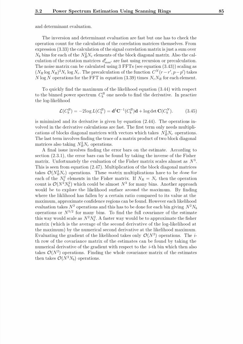
8/3/2019 Frode Kristian Hansen- Data Analysis of the Cosmic Microwave Background
http://slidepdf.com/reader/full/frode-kristian-hansen-data-analysis-of-the-cosmic-microwave-background 93/216
3.2 Power Spectrum Estimation Using Scanning Rings 85
and determinant evaluation.
The inversion and determinant evaluation are fast but one has to check theoperation count for the calculation of the correlation matrices themselves. Fromexpression (3.33) the calculation of the signal correlation matrix is just a sum overN b bins for each of the N 2RN r elements of the block diagonal matrix. Also the cal-
culation of the rotation matrices dmm are fast using recursion or precalculation.The noise matrix can be calculated using 3 FFTs (see equation (3.43)) scaling as(N R log N R)2N r log N r. The precalculation of the function C N (r −r, p− p) takesN log N operations for the FFT in equation (3.39) times N rN R for each element.
To quickly find the maximum of the likelihood equation (3.44) with respectto the binned power spectrum C Bb one needs to find the derivative. In practicethe log-likelihood
L(C Bb ) = −2log L(C Bb ) = d†C−1(C Bb )d + log det C(C N b ). (3.45)
is minimized and its derivative is given by equation (2.44). The operations in-volved in the derivative calculations are fast. The first term only needs multipli-cations of blocks diagonal matrices with vectors which takes N 2RN r operations.The last term involves finding the trace of a matrix product of two block diagonalmatrices also taking N 2RN r operations.
A final issue involves finding the error bars on the estimate. According tosection (2.3.1), the error bars can be found by taking the inverse of the Fishermatrix. Unfortunately the evaluation of the Fisher matrix scales almost as N 3.This is seen from equation (2.47). Multiplication of the block diagonal matricestakes O(N 3RN r) operations. These matrix multiplications have to be done for
each of the N
2
b elements in the Fisher matrix. If N R = N r then the operationcount is O(N 2N 2b ) which could be almost N 3 for many bins. Another approachwould be to explore the likelihood surface around the maximum. By findingwhere the liklihood has fallen by a certain ratio compared to its value at themaximum, approximate confidence regions can be found. However each likelihoodevaluation takes N 2 operations and this has to be done for each bin giving N 2N boperations or N 5/2 for many bins. To find the full covariance of the estimatethis way would scale as N 2N 2b . A faster way would be to approximate the fishermatrix (which is the average of the second derivative of the log-likelihood atthe maximum) by the numerical second derivative at the likelihood maximum.Evaluating the gradient of the likelihood takes only
O(N 2) operations. The i-
th row of the covariance matrix of the estimates can be found by taking thenumerical derivative of the gradient with respect to the i-th bin which then alsotakes O(N 2) operations. Finding the whole covariance matrix of the estimatesthen takes O(N 2N b) operations.

8/3/2019 Frode Kristian Hansen- Data Analysis of the Cosmic Microwave Background
http://slidepdf.com/reader/full/frode-kristian-hansen-data-analysis-of-the-cosmic-microwave-background 94/216
3.2 Power Spectrum Estimation Using Scanning Rings 86
3.2.2 An Example
Figure 3.5: The noise power spectrum used in the simulation. The vertical lineshows the knee frequency. The frequency k is shown in units of the Nyquistfrequency N T OD/2.
To test the above method for power spectrum estimation I simulated an ex-ample where N r = N R = 243 meaning that there are 243 scanning rings with 243pixels in each. Each ring is only scanned once N c = 1 so that the total numberof pixels N T OD = 59049, a similar number of pixels to the BOOMERANG ex-periment. The opening angle θE = 5 and the radius of each ring θ = 5. Allthe rings intersect at C (figure (3.1)). For simplicity a symmetric Gaussian beamwith 18 FWHM was used. This is however not necessary as the method can dealwith any beam pattern. The noise power spectrum was of the form (2.8) withα = 1. Writing P (k) in terms of wavenumber k one has
P (k) = σ2
1 + kknee
k
, (3.46)
with σ = 9µK and kknee = 4.3 × 10⁻³ in units of the Nyquist frequency N T OD/2.The power spectrum is showed in figure (3.5). With this noise model, the signal

8/3/2019 Frode Kristian Hansen- Data Analysis of the Cosmic Microwave Background
http://slidepdf.com/reader/full/frode-kristian-hansen-data-analysis-of-the-cosmic-microwave-background 95/216
3.2 Power Spectrum Estimation Using Scanning Rings 87
to noise ratio was one at a multipole of about = 600.
The simulation was carried out with the following steps:
1. First a standard CDM power spectrum was selected and a timestream wassimulated using the Wandelt-Gorski method described in section (3.1). Aset of ams were created using a random number generator and the CDMpower spectrum up to a multipole L = 1024. Then with equation (3.12)the Fourier transformed time stream was created and finally equation (3.14)(FFT) was used to create the time stream in pixel space. The ringset isshown in figure (3.6).
Figure 3.6: The ringset from a scan on a simulated sky without noise. On the plot
a line from the bottom to the top describes one ring. In this way the rings areput next to each other from the left to the right. The central point C where allrings intersect corresponds to the horizontal line of constant value in the middleof the plot.
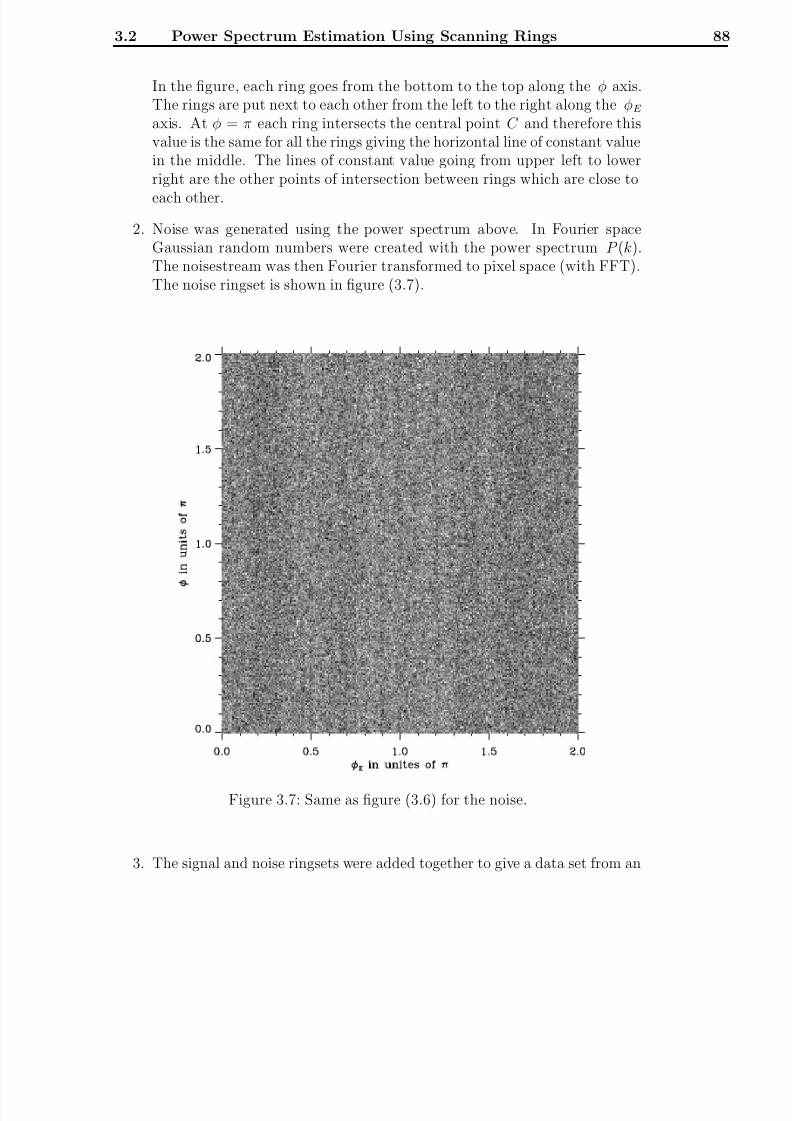
8/3/2019 Frode Kristian Hansen- Data Analysis of the Cosmic Microwave Background
http://slidepdf.com/reader/full/frode-kristian-hansen-data-analysis-of-the-cosmic-microwave-background 96/216
3.2 Power Spectrum Estimation Using Scanning Rings 88
In the figure, each ring goes from the bottom to the top along the φ axis.The rings are put next to each other from the left to the right along the φE
axis. At φ = π each ring intersects the central point C and therefore thisvalue is the same for all the rings giving the horizontal line of constant valuein the middle. The lines of constant value going from upper left to lowerright are the other points of intersection between rings which are close to
each other.
2. Noise was generated using the power spectrum above. In Fourier spaceGaussian random numbers were created with the power spectrum P (k).The noisestream was then Fourier transformed to pixel space (with FFT).The noise ringset is shown in figure (3.7).
Figure 3.7: Same as figure (3.6) for the noise.
3. The signal and noise ringsets were added together to give a data set from an

8/3/2019 Frode Kristian Hansen- Data Analysis of the Cosmic Microwave Background
http://slidepdf.com/reader/full/frode-kristian-hansen-data-analysis-of-the-cosmic-microwave-background 97/216
3.2 Power Spectrum Estimation Using Scanning Rings 89
experiment scanning on rings. The ringset is shown in figure (3.8). This isthe input data from which the power spectrum was to be estimated. Fromthe figure the vertical striping caused by the noise which was discussed insection (2.2.1) is clearly visible.
Figure 3.8: Same as figure (3.6) for signal plus noise. This is the result of addingthe ringsets in figure (3.6) and (3.7)
4. Now the simulated data set was used for likelihood estimation. A conju-gate gradient solver using only first derivative to find the minimum of thelog-likelihood was used (Press, Teukolsky, Vetterling, and Flannery 1992).Since the solver can easier handle a solution in which all the parametershave roughly the same order of magnitude, the following change of variableswas made:
C =Dbe−σ2
b(+1)
( + 1), (3.47)

8/3/2019 Frode Kristian Hansen- Data Analysis of the Cosmic Microwave Background
http://slidepdf.com/reader/full/frode-kristian-hansen-data-analysis-of-the-cosmic-microwave-background 98/216
3.2 Power Spectrum Estimation Using Scanning Rings 90
where Db is the binned power spectrum (b is bin number) for which thelog-likelihood was minimized. The Gaussian beam has σ = σb. For thisminimization 20 bins with 50 multipoles in each were used. The startingguess for the minimizer was Db = 104(µK )2 for all b = [0, 19]. For this testthe correlation matrix was calculated in pixel space (equation 3.22) andthen Fourier transformed using FFT. With the binning, equation (3.22)
takes the form
C S pr,pr =
b
Db
b
e−σ2b
(+1)
( + 1)
2 + 1
4πP (cos δθ), (3.48)
and its derivative is
∂C S pr,pr
∂Db=b
e−σ2b
(+1)
( + 1)
2 + 1
4πP (cos δθ), (3.49)
where the sum over b is the sum over all multipoles in the bin b. The
angles δθ between all possible pairs of points pr and p
r
were precalculated.5. After about 30 likelihood and derivative evaluations taking about 2 hours
each on a single processor on a 500MHz DEC Alpha Work Station theminimum was found. If the initial guess was better (it could have beentaken from a faster approximate power spectrum estimation algorithm asdiscussed in section (2.3)), the number of likelihood evaluations could havebeen significantly reduced. The result is shown in figure (3.9). The solidline is the input average power spectrum and the crosses are the estimatedbins. The crosses are plotted in the middle of each bin.

8/3/2019 Frode Kristian Hansen- Data Analysis of the Cosmic Microwave Background
http://slidepdf.com/reader/full/frode-kristian-hansen-data-analysis-of-the-cosmic-microwave-background 99/216
3.2 Power Spectrum Estimation Using Scanning Rings 91
Figure 3.9: The figure shows the result of the likelihood maximisation using theFourier transformed ringset as input data. The solid line shows the input averagepower spectrum and the crosses show the estimated bins with error bars. Theerror bars are approximate asymmetric 2σ confidence regions showing where thelog-likelihood drops by 2 compared to the maximum.
6. Finally the error bars were found. First the 2σ (95%) confidence regionswere found by finding where the log-likelihood had been reduces by 2 com-pared to the maximum. These asymmetric error bars are plotted on theestimates in figure (3.9). Then these error bars were compared to the 2σerror bars found from approximating the Fisher matrix by taking the numer-ical second derivative of the log-likelihood. These error bars were consistentwith the ones found from the likelihood contours.
3.2.3 Discussion
The power spectrum estimation method described here is the first exact methodwhich takes into account all the following effects:
• Correlated noise As discussed in previous sections, most CMB experi-ment have correlated noise. This can usually be seen in the CMB maps

8/3/2019 Frode Kristian Hansen- Data Analysis of the Cosmic Microwave Background
http://slidepdf.com/reader/full/frode-kristian-hansen-data-analysis-of-the-cosmic-microwave-background 100/216
3.2 Power Spectrum Estimation Using Scanning Rings 92
as stripes. Taking noise correlations into account when estimating thepower spectrum is usually hard and involves time consuming calculationsor Monte Carlo simulations. When operating on the timestream instead of the sky map, the noise correlations have a much simpler structure and arefor this reason easily incorporated into the power spectrum estimation bythe method described here.
• Non-uniform distribution of integration time Most CMB sky exper-iments do not observe each point on the sky the same amount of time. Forthis reason the noise for each point on a sky map will be different. On thetimeline integration time per pixel is by definition constant.
• Beam distortions and far side lobes Normally the beam of the tele-scope is approximated to be azimuthally symmetric and Gaussian. Thisis however not the case for all CMB experiments. Also diffraction of themicrowave radiation around the telescope and other apparatus used for theCMB experiment usually leads to far side lobes.
• Partial sky coverage Normally only parts of the sky are observed. Thisleads to coupling between the power spectrum coefficients C on the cutsky. These couplings have to be taken into account when attempting toestimate the full sky power spectrum from partial sky data.
• Pixelization effects When the CMB data are mapped before the powerspectrum estimation is performed, there is an additional smoothing of theCMB fluctuations on small scales due to the finite sized pixels in the map.On the method presented here, the CMB data is not mapped and hencethis effect is not present.
The MAP mission is design in such a way that the noise correlations are keptat a minimum. For this case there already exist fast methods for power spectrumestimation (Oh, Spergel, and Hinshaw 1999; Wandelt, Hivon, and Gorski 2000).These methods take into account most of the above mentions effect. They dohowever not take into account a non-symmetric beam shape and far side lobes. If these issues appear to be important then the method presented here is importantfor exact estimation of the power spectrum.
For the MAP mission and possibly for the Planck mission, the spin axis willbe precessing. In this case the centre of the scanning rings will not have thesame ΘE . One more rotation has to be added to equation (3.5) describing this
precession. For a precessing experiment where the amplitude of the precessions(variations in θE ) is given by the angle θP , the formula for the Fourier transformof the signal takes the following form
dS mmm =
amdmm(θE )d
mm(θP )X ∗m. (3.50)

8/3/2019 Frode Kristian Hansen- Data Analysis of the Cosmic Microwave Background
http://slidepdf.com/reader/full/frode-kristian-hansen-data-analysis-of-the-cosmic-microwave-background 101/216
3.2 Power Spectrum Estimation Using Scanning Rings 93
Obviously the correlation matrix < dmmmdM M M > is still block diagonal butthe blocks are now larger.
Another problem with the full sky experiment is that parts of the sky (aroundthe galactic plane) has to be cut out due to foreground contamination. This isequivalent to cutting out parts of the rings which destroys the symmetries making
the fast likelihood evaluation possible.
The power spectrum estimation method on rings, the way it is describedhere is clearly for an ideal experiment where there are no foregrounds and noirregularities in the scanning strategy. In reality however this will often notbe the case. To deal with these problems the method could be extended usingtechniques similar to those described in (Oh, Spergel, and Hinshaw 1999) andoutlined in section (2.3.1). The idea is that if one knows the exact solution in theideal situation then the case with cut rings and imperfect scanning strategy canbe considered as perturbations around the ideal case. In this way one can findthe product C−1d without having to invert C. As described in section (2.3.1)this can be done by preconditioned conjugate gradient techniques. By usingthe approximate C−1 by the methods described here one can iterate to find thecorrect C−1d without having to invert the full matrix C. This is delayed to futurework.

8/3/2019 Frode Kristian Hansen- Data Analysis of the Cosmic Microwave Background
http://slidepdf.com/reader/full/frode-kristian-hansen-data-analysis-of-the-cosmic-microwave-background 102/216
3.2 Power Spectrum Estimation Using Scanning Rings 94

8/3/2019 Frode Kristian Hansen- Data Analysis of the Cosmic Microwave Background
http://slidepdf.com/reader/full/frode-kristian-hansen-data-analysis-of-the-cosmic-microwave-background 103/216
Chapter 4
Gabor Transforms on the Sphere
and Application to CMB
Analysis
In this and the next chapter I will present work done under supervision of KrisGorski. In this chapter the formalism of windowed Fourier transforms known asGabor transforms is extended from the one dimesnional line to the sphere. TheGabor coefficients on the CMB sky will be studied and it is shown how theserepresent a compression of CMB data which allow for fast likelihood estimation.
Gabor transforms, or windowed Fourier transforms are just Fourier trans-forms where the function f (x) to be Fourier transformed is multiplied with aGabor Window W (x) (Gabor 1946). In the discrete case f (xi) can be a data set.If parts of the data set are of poor quality or are missing, this can be represented
as W (xi)f (xi) where the window W is zero where there are missing parts. Thewindow can also be formed so that it smooths the edges close to the missing partsand in this way avoid ringing in the Fourier spectrum.
In the first part of this chapter I will study the effect of Gabor transforms onthe sphere in particular for the CMB sky. The Gabor transform in this context is
just the multiplication of the CMB sky with a window function before using thespherical harmonic transform to get the pseudo power spectrum. The window canbe a tophat to take out certain parts of the sky for limited sky coverage. Anotherwindow can be a Gaussian Gabor window for smoothing the transition betweenthe observed and unobserved area of the sky. The Gabor window can also be
designed in such a way as to reduce signal-to-noise by giving pixels with highsignal-to-noise higher significance in the analysis. In the first part I will focus ontwo types of Gabor windows, the Gaussian window and the tophat window. Theeffect of these two windows will be compared. For a given patch on the sphere,the effect of multiplying this patch with a Gaussian to smooth the edges instead

8/3/2019 Frode Kristian Hansen- Data Analysis of the Cosmic Microwave Background
http://slidepdf.com/reader/full/frode-kristian-hansen-data-analysis-of-the-cosmic-microwave-background 104/216
96
of keeping it as a tophat with sharp edges will be discussed. I will show how theGaussian window cuts of long range correlations between the power spectrumcoefficients on the cut sphere (pseudo power spectrum) at the cost of increasedshort range correlations. The use of the windowed Fourier transform was alreadystudied in (Hobson and Magueijo 1996) in the flat sky approximation. I showthat some of their qualitative results are also valid on the sphere.
In (Hivon et al. 2001) the pseudo power spectrum was used as a quadraticestimator for CMB power spectrum analysis. In the second part of the chapterI will discuss the use of the pseudo power spectrum as a compression of a CMBdata set to be used in likelihood estimation. This was already done for a tophatwindow in (Wandelt, Hivon, and Gorski 2000) under the assumption that thepseudo spectrum coefficients are not coupled so that the correlation matrix forthe likelihood is diagonal. This is only a good assumption when a large part of the sky is covered. As I will show here, the couplings between the pseudo powerspectrum coefficients can be quite large depending on the size of the observedarea. For this reason the full covariance matrix will be used. Analytical andrecursive techniques will be developed which allows one to do fast calculation of the full covariance matrix.
The distribution of the pseudo power spectrum coefficients will be assumedGaussian. Using a Gaussian likelihood ansatz the full sky power spectrum willbe estimated from the noisy pseudo power spectrum. The likelihood functioncan in this case easily be calculated as the datavector and thereby the correla-tion matrix are small (only having a few hundres of elements even if the originalwhole data set had millions of pixels). The likelihood evaluation takes of theorder (N bin)2(N in)2 where N bin is the number of C bins estimated and N in is
the number of pseudo spectrum coefficients used as input to the likelihood. Themost time consuming part is the precomputation of some factors which scales asabout l3max for the signal part. For the noise correlation matrix this precalcula-
tion takes of the order
N pixlmax(N in)2 for axissymmetric noise or up to about N pixl2max(N in)2 for general noise. Typically N in ∝ lmax with a prefactor which
is dependent on the size of the window. For a 18 degree radius with Gaussianapodisation which will be used in some examples here N in ≈ 0.1lmax. Calcula-tions of noise prefactors can also be done by Monte-Carlo. It then takes of theorder N
3/2 pix N sim, where N sim is the number of Monte Carlo simulations needed,
which is typically a few thousand.
The method is developed for uncorrelated noise on an axissymmetric patch onthe sky. In the last part of the chapter extensions to non-symmetric patches andcorrelated noise will be worked out and further developments will be discussed.

8/3/2019 Frode Kristian Hansen- Data Analysis of the Cosmic Microwave Background
http://slidepdf.com/reader/full/frode-kristian-hansen-data-analysis-of-the-cosmic-microwave-background 105/216
4.1 The Gabor Transformation and the Temperature Power Spectrum 97
4.1 The Gabor Transformation and the Tem-
perature Power Spectrum
In this section I will first describe the Gabor transform for functions on a onedimensional line. Then I extend the formalism to functions on the sphere andthe properties of the Gabor transform coefficients on the sphere are discussed.
4.1.1 The One Dimensional Gabor Transform
For a data set d j with N elements, the normal Fourier transform is defined as,
dk =
j
d jei2πjk/N . (4.1)
A tilde on d shows that these are the Fourier coefficients. The inverse transformis then,
d j =
1
N k
˜dke
−i2πjk/N
. (4.2)
Sometimes it is useful to study the spectrum of just a part of the data set. Thiscould be if parts of it are of poor quality or the spectrum is changing along thedata set. In this case, one can multiply the data set with a function, removingthe unwanted parts and taking out a segment to be studied. The function can bea step function cutting out the segment to study with sharp edges or a functionwhich smooths the edges of the segment to avoid ringing (typically a Gaussian).
The Fourier transform with such a multiplication was studied by Gabor (Ga-bor 1946) and is called the Gabor Transform . It is defined for a segment centered
at j = M and with wavenumber k as,
dkM =
j
d jG j−M ei2πjk/N . (4.3)
Here G j−M is the Gabor Window , the function to multiply the data set with. Thetransform is similar to the Wavelet transform. The difference is that the windowfunction in the Wavelet transform is frequency dependent so that the size of thesegment is changing with frequency.
Analogously to the Fourier transform, there is also an inverse Gabor trans-
form. To recover the whole data set from a Gabor transform, one needs theFourier coefficients taken with different windows G j−M being centered at severaldifferent points M . This means that the data set has to be split up into severalsegments. The center of each segment is set to M = mK where K determines

8/3/2019 Frode Kristian Hansen- Data Analysis of the Cosmic Microwave Background
http://slidepdf.com/reader/full/frode-kristian-hansen-data-analysis-of-the-cosmic-microwave-background 106/216
4.1 The Gabor Transformation and the Temperature Power Spectrum 98
the density of segments and m is an integer specifying the segment number. Onethen has for the inverse transform
d j =
m
k
dkmgkm. (4.4)
Due to the non-orthogonality of the Gabor transform, the dual Gabor window gkm
is not trivial to find, but several techniques have been developed for calculatingthis dual window (e.g. (Strohmer 1997) and references therein).
In this chapter I will study the Gabor transform on the sphere and apply itto CMB analysis. I will take out a disc on the CMB sky, using either tophator Gaussian apodisation and then create the pseudo power spectrum C on thisapodised sky. These C will be used for likelihood estimation of the underlyingfull sky power spectrum. I also outline how several discs (segments) centered atdifferent points can be combined to yield the full sky power spectrum.
4.1.2 Gabor Transform on the Sphere
I start by defining the C for a Gabor Window G(n) as,
C =
m
a∗mam
2 + 1, (4.5)
wheream =
dnT (n)G(n)Y ∗m(n). (4.6)
Here T (n) is the observed temperature in the direction of the unit vector n,Y m(n) is the spherical Harmonic function and G(n) is the Gabor window.
I will here use a Gabor Window which is azimuthally symmetric about a pointn0 on the sphere, so that the window is only a function of the angular distance
from this point on the sphere cos θ = n · n0. Then one can write the Legendreexpansion of the window as,
G(θ) =
2 + 1
4πgP (cos θ) =
m
gY m(n)Y ∗m(n0). (4.7)
One can also write,T (n) =
m
amY m(n). (4.8)
Inserting these two expressions in equation (4.6) one gets
am = m
am
m
gY ∗m(n0) Y ∗m(n)Y m(n)Y m(n)dn (4.9)
=m
am
m
gY ∗m(n0)
(2 + 1)(2 + 1)(2 + 1)
4π(4.10)
×
−m m m
0 0 0
(−1)m, (4.11)
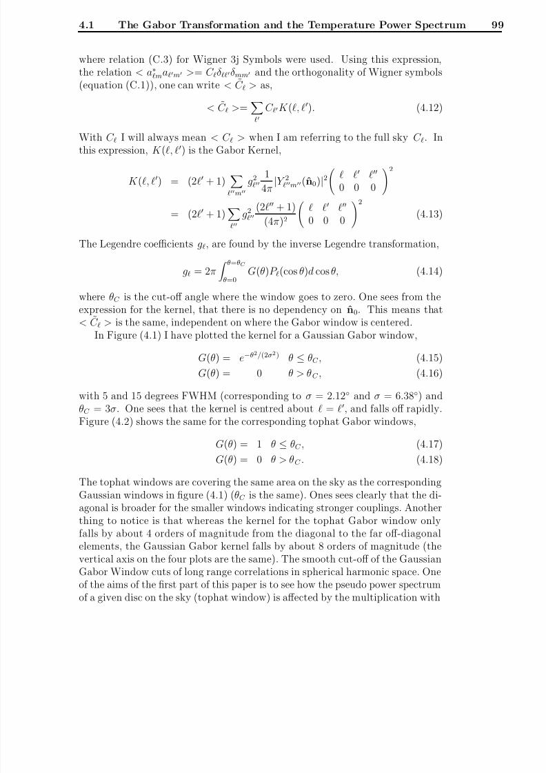
8/3/2019 Frode Kristian Hansen- Data Analysis of the Cosmic Microwave Background
http://slidepdf.com/reader/full/frode-kristian-hansen-data-analysis-of-the-cosmic-microwave-background 107/216
4.1 The Gabor Transformation and the Temperature Power Spectrum 99
where relation (C.3) for Wigner 3j Symbols were used. Using this expression,the relation < a∗mam >= C δδmm and the orthogonality of Wigner symbols(equation (C.1)), one can write < C > as,
< C >=
C K (, ). (4.12)
With C I will always mean < C > when I am referring to the full sky C . Inthis expression, K (, ) is the Gabor Kernel,
K (, ) = (2 + 1)
m
g21
4π|Y 2m(n0)|2
0 0 0
2
= (2 + 1)
g2(2 + 1)
(4π)2
0 0 0
2
(4.13)
The Legendre coefficients g, are found by the inverse Legendre transformation,
g = 2π θ=θC
θ=0 G(θ)P (cos θ)d cos θ, (4.14)
where θC is the cut-off angle where the window goes to zero. One sees from theexpression for the kernel, that there is no dependency on n0. This means that< C > is the same, independent on where the Gabor window is centered.
In Figure (4.1) I have plotted the kernel for a Gaussian Gabor window,
G(θ) = e−θ2/(2σ2) θ ≤ θC , (4.15)
G(θ) = 0 θ > θC , (4.16)
with 5 and 15 degrees FWHM (corresponding to σ = 2.12 and σ = 6.38) and
θC = 3σ. One sees that the kernel is centred about = , and falls off rapidly.Figure (4.2) shows the same for the corresponding tophat Gabor windows,
G(θ) = 1 θ ≤ θC , (4.17)
G(θ) = 0 θ > θC . (4.18)
The tophat windows are covering the same area on the sky as the correspondingGaussian windows in figure (4.1) (θC is the same). Ones sees clearly that the di-agonal is broader for the smaller windows indicating stronger couplings. Anotherthing to notice is that whereas the kernel for the tophat Gabor window onlyfalls by about 4 orders of magnitude from the diagonal to the far off-diagonalelements, the Gaussian Gabor kernel falls by about 8 orders of magnitude (thevertical axis on the four plots are the same). The smooth cut-off of the GaussianGabor Window cuts of long range correlations in spherical harmonic space. Oneof the aims of the first part of this paper is to see how the pseudo power spectrumof a given disc on the sky (tophat window) is affected by the multiplication with
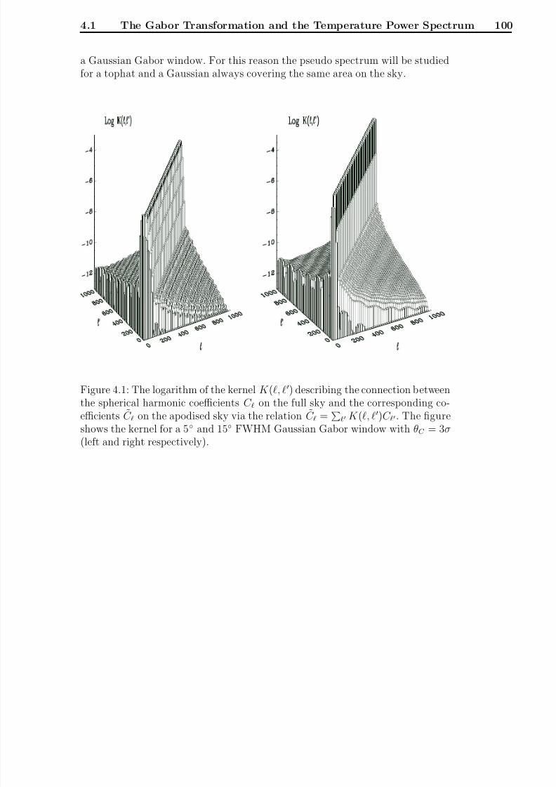
8/3/2019 Frode Kristian Hansen- Data Analysis of the Cosmic Microwave Background
http://slidepdf.com/reader/full/frode-kristian-hansen-data-analysis-of-the-cosmic-microwave-background 108/216
4.1 The Gabor Transformation and the Temperature Power Spectrum 100
a Gaussian Gabor window. For this reason the pseudo spectrum will be studiedfor a tophat and a Gaussian always covering the same area on the sky.
Figure 4.1: The logarithm of the kernel K (, ) describing the connection betweenthe spherical harmonic coefficients C on the full sky and the corresponding co-
efficients C on the apodised sky via the relation C = K (, )C . The figure
shows the kernel for a 5 and 15 FWHM Gaussian Gabor window with θC = 3σ(left and right respectively).

8/3/2019 Frode Kristian Hansen- Data Analysis of the Cosmic Microwave Background
http://slidepdf.com/reader/full/frode-kristian-hansen-data-analysis-of-the-cosmic-microwave-background 109/216
4.1 The Gabor Transformation and the Temperature Power Spectrum 101
Figure 4.2: Same as figure (4.1) for tophat Gabor windows covering the samearea on the sky as the Gaussian windows.
In figure (4.3), I have plotted cuts through the kernel at = 200 and = 500for the 5 and 15 degree FWHM Gaussian Gabor windows (dashed line). The solidline is the corresponding kernel (same area on the sky) when using the tophatGabor window. One sees that the Gaussian window effectively cuts of long rangecorrelations whereas the tophat window is narrower close to the diagonal. TheGaussian window has larger short range correlations.

8/3/2019 Frode Kristian Hansen- Data Analysis of the Cosmic Microwave Background
http://slidepdf.com/reader/full/frode-kristian-hansen-data-analysis-of-the-cosmic-microwave-background 110/216
4.1 The Gabor Transformation and the Temperature Power Spectrum 102
Figure 4.3: The figures show cuts through the kernel K (, ) connecting the fullsky and cut sky spherical harmonic coefficients. The full kernels are shown in
figures (4.1) and (4.2). The cuts are taken at = 200 and = 500 for the 5 (upperplot) and 15 (lower plot) degree Gaussian Gabor window (dashed line). The solidline is for the corresponding (same area on the sky) tophat window. The kernelsare here normalised so that the peak at the given cut has its maximum at 1. Inthis way one can easier compare the kernels.
Figure (4.4) shows how the width of the kernel gets narrower and the corre-lations smaller as the Gabor window opens up. The four kernels are shown for = 500 and the Gaussian windows have 5, 10, 15 and 30 degree FWHM with
θC = 3σ. The same relation for the corresponding (in the sense described above)tophat window is also shown. Gaussian functions are plotted on top of the kernelsand show that the kernels are very close to Gaussian functions near the diagonal.

8/3/2019 Frode Kristian Hansen- Data Analysis of the Cosmic Microwave Background
http://slidepdf.com/reader/full/frode-kristian-hansen-data-analysis-of-the-cosmic-microwave-background 111/216
4.1 The Gabor Transformation and the Temperature Power Spectrum 103
Figure 4.4: The figures show a cut through the kernel K (, ) connecting the fullsky and cut sky spherical harmonic coefficients. The cuts are taken at = 500for a 5, 10, 15 and 30 degree FWHM Gaussian Gabor window (solid line) with aθC = 3σ cut-off. The dotted line shows the kernel for a tophat window coveringthe same area on the sky. Dashed lines are Gaussian fits to the curves.
In figure (4.5) I have plotted the relation between the FWHM width ∆ of
the kernel and the size ∆θ of the window for Gaussian and tophat windows.The two curves are very well described by ∆ = 220/θF W H M for the Gaussianwindow (θF W H M in degrees) and ∆ = 140/θF W H M for the corresponding tophatwindow. Clearly for a given observed area of the sky, multiplying with a Gaussianwill increase the FWHM of the kernel. This is also what was seen in figure (4.3)

8/3/2019 Frode Kristian Hansen- Data Analysis of the Cosmic Microwave Background
http://slidepdf.com/reader/full/frode-kristian-hansen-data-analysis-of-the-cosmic-microwave-background 112/216
4.1 The Gabor Transformation and the Temperature Power Spectrum 104
and (4.4).
Figure 4.5: The figure shows the uncertainty relation ∆∆θ = consant for a Ga-bor transform on the sphere. The solid line shows the width ∆ of the Gaborkernel K (, ) connecting the full sky and the cut sky power spectra when ap-plying a Gaussian Gabor window with a cut θC = 3σ. The FWHM is showed onthe lower abcissa. The dashed line shows the width of the kernel for a tophatwindow covering the same area of the sky as the Gaussian. The full radius of thetophat window is shown on the upper abcissa. The curves are well described by∆ = 220/θF W H M and ∆ = 140/θF W H M for the Gaussian and tophat windowsrespectively.
In Figure (4.6), I show the shapes of the C for Gaussian and tophat win-dows compared to the full sky spectrum. The plots which were made using theanalytical formula (4.12) show C for a 5 and 15 degree FWHM Gaussian Gaborwindow (solid line) cut at 3σ. The corresponding spectra for the tophat Gaborwindows are shown as dotted lines. The spectra are normalised in such a way that

8/3/2019 Frode Kristian Hansen- Data Analysis of the Cosmic Microwave Background
http://slidepdf.com/reader/full/frode-kristian-hansen-data-analysis-of-the-cosmic-microwave-background 113/216
4.1 The Gabor Transformation and the Temperature Power Spectrum 105
they can be compared to the full sky power spectrum (dashed line). For the 5
FWHM window one can still distinguish the three lines. At this window size thepseudo spectra are very similar to the full sky spectra but with small deviationsdepending on the shapes of the kernel and the shape of the power spectrum. Inthis case the spectrum for the Gaussian window seems to be smaller at the peaksand larger at the troughs whereas the spectrum for the tophat window is always
larger. For the 15 FWHM windows the pseudo spectrum using the GaussianGabor window are on top of the full sky power spectrum. For the tophat windowit is still possible to distinguish the pseudo spectrum from the full sky powerspectrum although the lines are still very close. This means that the C couldbe good estimators of the underlying full sky C provided that the window is bigenough. This is consistent with the conclusion in (Hobson and Magueijo 1996),where this was shown in the flat sky approximation.
One feature which is very prominent is the additional peak at low for theGaussian window. The reason for this peak comes from the fact that the diagonalin the Gaussian kernel is broader than in the tophat kernel. For the low multipolesthe power spectrum is dropping rapidly because of the Sachs-Wolfe effect and thelowest multipole C are much bigger than the C for higher multipoles. Since theGaussian kernel is broad, the C at low multipoles will pick up more from theC at lower multipoles than the narrower tophat kernel (see figure (4.3). Theselow multipole C have very high values compared to the higher multipole C andfor that reason the C for the Gaussian window will get a higher value. This isillustrated in figure (4.7) where a cut through the kernel at = 50 is shown forthe 5 FWHM Gaussian Gabor window (solid line) and the corresponding tophat(dashed line) normalised to one at the peak. The dotted line shows a typicalpower spectrum. Clearly the Gaussian kernel will pick up more of the high value
C at low multipoles.

8/3/2019 Frode Kristian Hansen- Data Analysis of the Cosmic Microwave Background
http://slidepdf.com/reader/full/frode-kristian-hansen-data-analysis-of-the-cosmic-microwave-background 114/216
4.1 The Gabor Transformation and the Temperature Power Spectrum 106
Figure 4.6: The windowed power spectra C for a 5 and 15 degree FWHM Gaus-sian Gabor Gabor window cut at θC = 3σ (solid line) and for a tophat window
covering the same area on the sky (dotted line). All spectra are normalised insuch a way that they can be compared directly with the full sky spectrum whichis shown on each plot as a dashed line. Only in the first plot are all three linesvisible. In the three last plots, the full sky spectrum and the Gaussian pseudospectrum (dashed and solid line) are only distinguishable in the first few multi-poles.
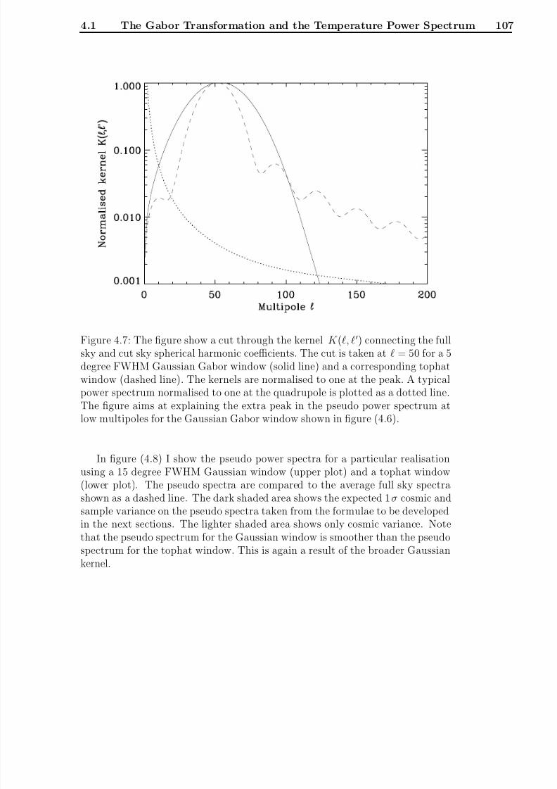
8/3/2019 Frode Kristian Hansen- Data Analysis of the Cosmic Microwave Background
http://slidepdf.com/reader/full/frode-kristian-hansen-data-analysis-of-the-cosmic-microwave-background 115/216
4.1 The Gabor Transformation and the Temperature Power Spectrum 107
Figure 4.7: The figure show a cut through the kernel K (, ) connecting the fullsky and cut sky spherical harmonic coefficients. The cut is taken at = 50 for a 5degree FWHM Gaussian Gabor window (solid line) and a corresponding tophatwindow (dashed line). The kernels are normalised to one at the peak. A typicalpower spectrum normalised to one at the quadrupole is plotted as a dotted line.The figure aims at explaining the extra peak in the pseudo power spectrum at
low multipoles for the Gaussian Gabor window shown in figure (4.6).
In figure (4.8) I show the pseudo power spectra for a particular realisationusing a 15 degree FWHM Gaussian window (upper plot) and a tophat window(lower plot). The pseudo spectra are compared to the average full sky spectrashown as a dashed line. The dark shaded area shows the expected 1σ cosmic andsample variance on the pseudo spectra taken from the formulae to be developedin the next sections. The lighter shaded area shows only cosmic variance. Notethat the pseudo spectrum for the Gaussian window is smoother than the pseudo
spectrum for the tophat window. This is again a result of the broader Gaussiankernel.

8/3/2019 Frode Kristian Hansen- Data Analysis of the Cosmic Microwave Background
http://slidepdf.com/reader/full/frode-kristian-hansen-data-analysis-of-the-cosmic-microwave-background 116/216
4.1 The Gabor Transformation and the Temperature Power Spectrum 108
Figure 4.8: One realisation of the windowed power spectra. The upper plot showsa realisation of a pseudo power spectrum using a 15 degree FWHM Gaussian
Gabor window. The pseudo spectrum is normalised in such a way that it can becompared directly to the full sky spectrum which average is shown as a dottedline. The lower plot shows the same realisation using a corresponding tophatwindow. The ligh shaded area shows 1σ cosmic variance around the full skyaverage spectrum. The darker area shows 1σ cosmic and sampling variance takenfrom the theoretical formula.
4.1.3 Rotational Invariance
It was shown that the average <˜
C > is invariant under rotations of the Gaborwindow. I will now show that the non averaged C are rotationally invariantunder any rotation of the sky AND Gabor window by the same angle. This fact
justifies that I in the following always put the window on the north pole sincethis simplifies the calculations. In the following I will use the rotation matrices

8/3/2019 Frode Kristian Hansen- Data Analysis of the Cosmic Microwave Background
http://slidepdf.com/reader/full/frode-kristian-hansen-data-analysis-of-the-cosmic-microwave-background 117/216
4.1 The Gabor Transformation and the Temperature Power Spectrum 109
Dmm described in Appendix (A). Consider a rotation of the sky and window by
the angles (−γ − β − α). Then the am becomes,
arotm =
dn[D(−γ − β − α)T (n)G(n)]Y ∗m(n). (4.19)
If one makes the inverse rotation of the integration angle n, one can write this as
arotm = dnT (n)G(n)[D∗(αβγ )Y ∗m(n)], (4.20)
which is just
arotm =
m
D∗mm(αβγ )
dnT (n)G(n)Y ∗m(n). (4.21)
One can identify the last integral as the normal am.
arotm =
m
D∗mm(αβγ )am. (4.22)
So the am are NOT rotationally invariant. Rotation mixes m-modes for a given-value.
Now to the C l. One has that
C rot =
1
2 + 1
m
arotm arot*
m (4.23)
=1
2 + 1
m
m
m
Dmm(αβγ )D∗
mm(αβγ )ama∗m (4.24)
=1
2 + 1
mm
am a∗m
m
Dmm(αβγ )D∗
mm(αβγ ). (4.25)
Using the properties given in Appendix (A), one can write the last D-functionon the last line as,
D∗mm(αβγ ) = D
mm(−αβ − γ ) (4.26)
= e−imαdmm(β )e−imγ (4.27)
= e−imαdmm(−β )e−imγ (4.28)
= Dmm(−γ − β − α). (4.29)
Knowing that (−γ − β − α) is the inverse rotation of (αβγ ) one can write,m
Dmm(αβγ )D∗
mm(αβγ ) =
m
Dmm(αβγ )D
mm(−γ − β − α) (4.30)
= Dmm(000) = δmm (4.31)
So one gets,C rot
= C . (4.32)

8/3/2019 Frode Kristian Hansen- Data Analysis of the Cosmic Microwave Background
http://slidepdf.com/reader/full/frode-kristian-hansen-data-analysis-of-the-cosmic-microwave-background 118/216
4.2 Likelihood Analysis 110
4.2 Likelihood Analysis
In this section I will show how the pseudo power spectrum can be used as in-put to a likelihood analysis for estimating the full sky power spectrum from anobserved disc on the sky multiplied with a Gabor window. I will in this sectionconcentrate on a Gaussian Gabor window, but the formalism is valid for any
azimuthally symmetric Gabor window.
4.2.1 The Form of the Likelihood Function
To know the form of the likelihood function, one needs to know the probabilitydistribution of C . In Figure (4.9) and (4.10) I show the probability distribu-tion from 10000 simulations with a 5 and 15 FWHM Gaussian Gabor windowrespectively. The dashed line shows a Gaussian with mean value and standarddeviation found from the formulae given in the previous and next section. Onecan see that the probability distribution is slightly skewed for low , but for high
it seems to be very well approximated by a Gaussian. Also the small windowshows more deviations from a Gaussian than the bigger window. In figure (4.11) Ishow the probability distribution from a simulation with a tophat Gabor windowcovering the same area on the sky as the 15 FWHM Gaussian window. Also forthis window the probability distribution is close to Gaussian.
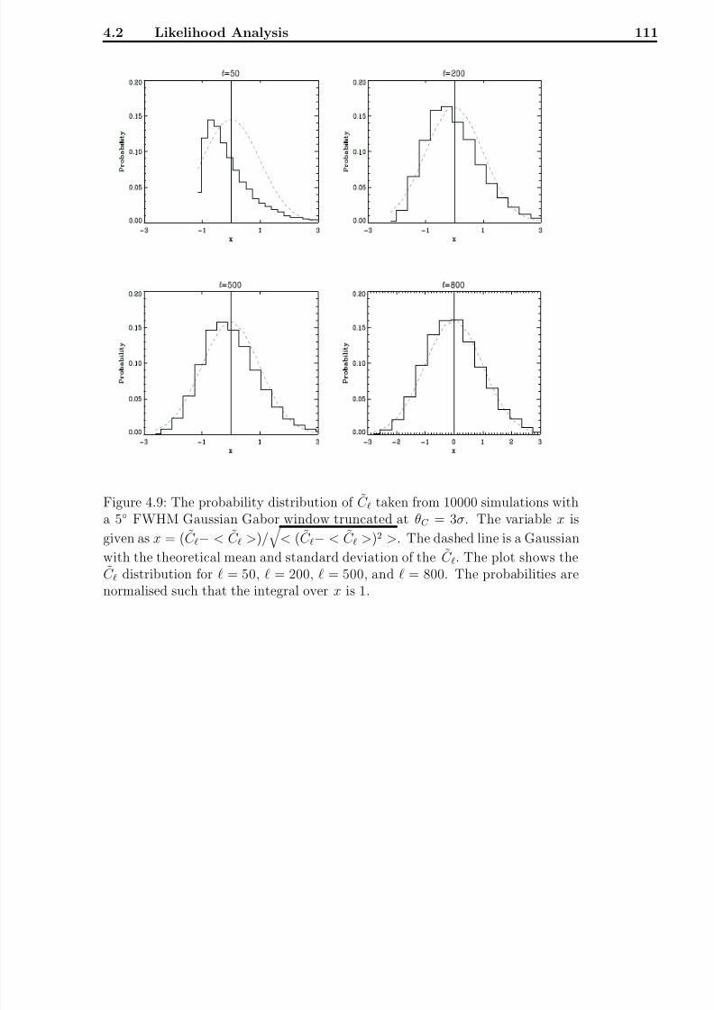
8/3/2019 Frode Kristian Hansen- Data Analysis of the Cosmic Microwave Background
http://slidepdf.com/reader/full/frode-kristian-hansen-data-analysis-of-the-cosmic-microwave-background 119/216
4.2 Likelihood Analysis 111
Figure 4.9: The probability distribution of C taken from 10000 simulations witha 5 FWHM Gaussian Gabor window truncated at θC = 3σ. The variable x is
given as x = (C − < C >)/
< (C − < C >)2 >. The dashed line is a Gaussian
with the theoretical mean and standard deviation of the C . The plot shows theC distribution for = 50, = 200, = 500, and = 800. The probabilities arenormalised such that the integral over x is 1.

8/3/2019 Frode Kristian Hansen- Data Analysis of the Cosmic Microwave Background
http://slidepdf.com/reader/full/frode-kristian-hansen-data-analysis-of-the-cosmic-microwave-background 120/216
4.2 Likelihood Analysis 112
Figure 4.10: Same as figure (4.9) but for a 15 FWHM Gaussian Gabor window.

8/3/2019 Frode Kristian Hansen- Data Analysis of the Cosmic Microwave Background
http://slidepdf.com/reader/full/frode-kristian-hansen-data-analysis-of-the-cosmic-microwave-background 121/216
4.2 Likelihood Analysis 113
Figure 4.11: Same as figure (4.10) but for a tophat Gabor window covering thesame area on the sky.
From the above plots it seems to be reasonable to approximate the likelihoodfunction with a Gaussian provided the window is big enough and multipoles athigh enough values are used,
L =e−
1
2dT M−1d
√2π det M
. (4.33)
Omitting all constant terms and factors, the log-likelihood can then be writ-ten:
L = dT M−1d + ln det M. (4.34)
Here d is the datavector which contains the observed C for the set of sample-values i. The datavector is taken from the observed windowed sky in the

8/3/2019 Frode Kristian Hansen- Data Analysis of the Cosmic Microwave Background
http://slidepdf.com/reader/full/frode-kristian-hansen-data-analysis-of-the-cosmic-microwave-background 122/216
4.2 Likelihood Analysis 114
following way:di = C i− < C i > . (4.35)
The matrix M is the covariance between pseudo-C l which elements are givenby:
M ij =< C iC j > − < C i >< C j > . (4.36)
The next step is to find an expression for M ij first assuming that no noise ispresent.
4.2.2 The Correlation Matrix
To do fast likelihood analysis with C one needs to be able to calculate < C > andthe correlations < C C > fast. Calculating the average < C > by formula (4.12)using the analytic expression (4.13) for the kernel is not very fast. It turns out thata faster way of evaluating the kernel is by using direct integration (summationon the pixelised sphere) and then, as shown in Appendix (D), recurrence. Bymeans of an integral, one can then write the am as (now assuming that n0 is onthe north pole),
am =m
am
G(n)Y ∗m(n)Y m(n)dn
=m
am
G(θ)λm(θ)λm(θ)d cos θ
e−iφ(m−m)dφ
2πδmm
=
am2π G(θ)λm(θ)λm(θ)d cos θ
≡
amh(, , m), (4.37)
where the last line defines h(, , m) and λm(θ) is given by,
Y m(θ, φ) = λm(θ)e−iφm. (4.38)
Using this form, one gets,
< C >=1
2 + 1 C
mh2(, , m). (4.39)
To obtain this expression, n0 was on the north pole, but as was shown, the< C >s are rotationally invariant, that is < C > remains the same if one ro-tates the Gabor window so that it is centered on the north pole.
8/3/2019 Frode Kristian Hansen- Data Analysis of the Cosmic Microwave Background
http://slidepdf.com/reader/full/frode-kristian-hansen-data-analysis-of-the-cosmic-microwave-background 123/216
4.2 Likelihood Analysis 115
When using real CMB data, the observed temperature map is always pixelised.So an integral over the sphere has to be replaced by a sum over pixels. In thiscase, the formula for h(, , m) has to be replaced by
h(, , m) =
j
G j λ jmλ j
m∆ j, (4.40)
where the index j is the pixel number replacing the angle θ and ∆ j is the areaof pixel j. Using a pixelisation scheme like HEALPix (Gorski et al. ) which hasa structure of azimuthal rings going from the north to the south pole with N rpixels in ring r and equal area for each pixel ∆ j = ∆ this can be written as
h(, , m) = ∆
r
N r−1 p=0
Grλrmλr
m,
= ∆
r
N rGrλrmλr
m. (4.41)
Here the sum over pixels is split into a sum over rings r and a sum over the pixels
in each ring p. The first sum goes over all rings which have θ < θC .Using this expression for the am one can now find the correlation matrix
< C C >=
mm
< a∗mama∗mam >
(2 + 1)(2 + 1). (4.42)
In this expression one can use relation (4.37) to get,
< C C > =1
(2 + 1)(2 + 1)
mm
LLKK
< a∗LmaLma∗KmaK m > (4.43)
×h(,L,m)h(, L, m)h(, K , m)h(, K , m) (4.44)
= 1(2 + 1)(2 + 1)
(4.45)
× mm
LLKK
[< a∗LmaLm >< a∗KmaK m > (4.46)
+ < a∗Lma∗Km >< aLmaK m > (4.47)
+ < a∗LmaK m >< aLma∗Km >] (4.48)
× h(,L,m)h(, L, m)h(, K , m)h(, K , m). (4.49)
Clearly the first term is just the product < C >< C >, and the two last termsare equal (using a∗Km = aKm(−1)m
and aK m = (−1)m
a∗K m) so one gets,
M ij =2
(2 + 1)(2 + 1)
m
L
C Lh(i, L , m)h( j, L , m)
2
. (4.50)
This is one of the main results of this thesis since the formula allows one to ana-lytically calculate the correlation matrix needed for likelihood analysis. Another
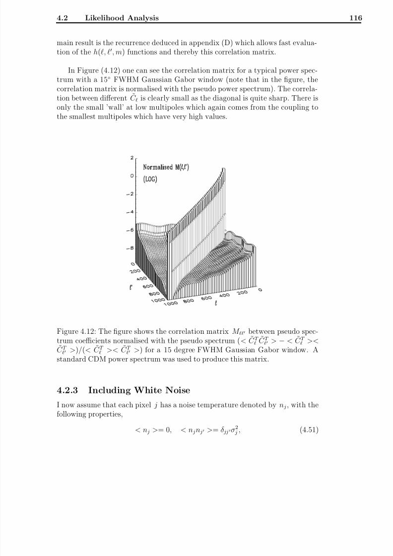
8/3/2019 Frode Kristian Hansen- Data Analysis of the Cosmic Microwave Background
http://slidepdf.com/reader/full/frode-kristian-hansen-data-analysis-of-the-cosmic-microwave-background 124/216
4.2 Likelihood Analysis 116
main result is the recurrence deduced in appendix (D) which allows fast evalua-tion of the h(, , m) functions and thereby this correlation matrix.
In Figure (4.12) one can see the correlation matrix for a typical power spec-trum with a 15 FWHM Gaussian Gabor window (note that in the figure, thecorrelation matrix is normalised with the pseudo power spectrum). The correla-
tion between different C is clearly small as the diagonal is quite sharp. There isonly the small ’wall’ at low multipoles which again comes from the coupling tothe smallest multipoles which have very high values.
Figure 4.12: The figure shows the correlation matrix M between pseudo spec-trum coefficients normalised with the pseudo spectrum (< C T
C T > − < C T
><C T
>)/(< C T >< C T
>) for a 15 degree FWHM Gaussian Gabor window. Astandard CDM power spectrum was used to produce this matrix.
4.2.3 Including White Noise
I now assume that each pixel j has a noise temperature denoted by n j , with thefollowing properties,
< n j >= 0, < n jn j >= δ jj σ2
j , (4.51)

8/3/2019 Frode Kristian Hansen- Data Analysis of the Cosmic Microwave Background
http://slidepdf.com/reader/full/frode-kristian-hansen-data-analysis-of-the-cosmic-microwave-background 125/216
4.2 Likelihood Analysis 117
where σ j is the noise variance in pixel j. Then one has the following expressionsfor the am and C l (I use superscript N for noise quantities),
aN m =
j
n j Y j∗m∆ j (4.52)
< aN maN
m
∗> = jj
< n jn j > Y jmY j
m
∗∆ j∆ j = j
σ2 j Y jmY jm
∗∆2
j (4.53)
< C N > =
1
2 + 1
m
< aN maN
m
∗>=
1
4π
j
σ2 j ∆2
j . (4.54)
Here Y jm is the Spherical Harmonic of the pixel centre of pixel j. For the win-dowed coefficients, one gets similarly,
aN m =
j
G jn j ∆ j Y j∗m (4.55)
C N =
1
4π
j
σ2 j G2
j ∆2 j (4.56)
The next step is to find the noise correlation matrix,
< C N C N
> =1
(2 + 1)(2 + 1)
mm
jj kk
∆ j∆ j∆k∆k (4.57)
× < n jn jnknk > G jG jGkGkY jmY j
mY kmY k
m (4.58)
= < C N >< C N
> +M N , (4.59)
where M N can be written as,
M N
=
2
(2 + 1)(2 + 1) mm
j ∆
2
j G2
j σ2
j Y
j
mY
j
m
∗2
(4.60)
For pixelisation schemes like HEALPix, the expression can be evaluated fast usingFFT. This is apparent when one writes the sum over pixels as a double sum overrings and pixels per ring.
j
∆2 j G2
j σ2 j Y jmY jm
∗=
r
ΛrmΛr
m
N r−1 p=0
e−iφp(m−m)∆2G2rσ2
r,p. (4.61)
In the case of an axissymmetric noise model, this expression becomes even easierwhich is apparent writing this as
r
ΛrmΛr
m∆2G2rσ2
r
N r−1 p=0
e−iφp(m−m)
N rδmm
= ∆
r
ΛrmΛr
m ∆Grσ2r
Gr
≡ h(, , m).
(4.62)
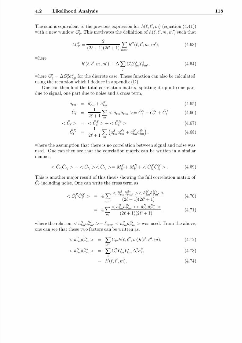
8/3/2019 Frode Kristian Hansen- Data Analysis of the Cosmic Microwave Background
http://slidepdf.com/reader/full/frode-kristian-hansen-data-analysis-of-the-cosmic-microwave-background 126/216
4.2 Likelihood Analysis 118
The sum is equivalent to the previous expression for h(, , m) (equation (4.41))with a new window G
r. This motivates the definition of h(, , m , m) such that
M N =
2
(2 + 1)(2 + 1)
mm
h2(, , m , m), (4.63)
where h(, , m , m) ≡ ∆
j
G jY jmY jm , (4.64)
where G j = ∆G2
rσ2r,p for the discrete case. These function can also be calculated
using the recursion which I deduce in appendix (D).One can then find the total correlation matrix, splitting it up into one part
due to signal, one part due to noise and a cross term,
am = aS m + aN
m (4.65)
C =1
2 + 1 m< amam >= C S
+ C N + C X (4.66)
< C > = < C S > + < C N
> (4.67)
C X =1
2 + 1
m
aS
maN ∗m + aN
maS ∗m
, (4.68)
where the assumption that there is no correlation between signal and noise wasused. One can then see that the correlation matrix can be written in a similarmanner,
< C iC j > − < C i >< C j >= M S ij + M N
ij + < C Xi C Xj > . (4.69)
This is another major result of this thesis showing the full correlation matrix of C including noise. One can write the cross term as,
< C X C X > = 4mm
< aS maS ∗
m >< aN maN ∗
m >
(2 + 1)(2 + 1)(4.70)
= 4
m
< aS maS ∗
m >< aN maN ∗
m >
(2 + 1)(2 + 1), (4.71)
where the relation < aS maS ∗
m >= δmm < aS maS ∗
m > was used. From the above,one can see that these two factors can be written as,
< aS ma
S ∗m > =
C h(,
, m)h(
,
, m), (4.72)
< aN maN ∗
m > =
i
G2i Y imY im∆2
i σ2i , (4.73)
= h(, , m). (4.74)

8/3/2019 Frode Kristian Hansen- Data Analysis of the Cosmic Microwave Background
http://slidepdf.com/reader/full/frode-kristian-hansen-data-analysis-of-the-cosmic-microwave-background 127/216
4.2 Likelihood Analysis 119
4.2.4 Likelihood Estimation and Results
The expressions for the covariance matrix and mean psuedo-C have now beenfound. Because of the limited information content in one patch of the sky onecan not estimate the full sky C for all multipoles . For this reason the full skypower spectrum has to be estimated in N bin bins. Also the algorithm to minimize
the log-likelihood needs the numbers to be estimated to be of roughly the sameorder of magnitude. For this reason I estimate for some parameters Db which forbin b is defined as
C =Db
( + 1), b ≤ < b+1, (4.75)
where b is the first multipole in bin b. Using this binning, one can calculate thelikelihood significantly faster by writing the signal correlation matrix equation(4.50) as
M S ij =
b
b
DbDbχ(b, b, i , j), (4.76)
where χ(b, b, i , j) is given as,
χ(b, b, i ,j) ≡ 2
(2i + 1)(2 j + 1)
× m
lb
B2 ( + 1)h(, i, m)h(, j, m)
×
lbB2
( + 1)h(, i, m)h(, j, m)
, (4.77)
which is precomputed. The sums over here go over the values in each specific
bin b. One sees that computing the likelihood takes of the order (N bin
)2
(N in
)2
op-erations whereas the precomputation of the factor χ(k, k, i , j) goes as (N bin)2(N in)2N mwhere N m is the number of m values used. Note that the multipole coefficientsof the beam B are also included. The reason is that the input data is alwaysaffected by the beam and this is corrected for by using the beam convolved fullsky power spectrum C B2
.
The sum over m in the expressions for the covariance matrix and < C > canbe limited. The h-functions are rapidly decreasing for increasing m for Gaussianand tophat windows. For Gaussian Gabor windows it seems that one can cut thesums over m at 200 to high accuracy. For top-hat windows, the sum should be
extended to m = 400.
The noise cross term can be written in a similar way as
M Xij ≡< C Xi C Xj >=
k
Dbχ(b,i,j), (4.78)

8/3/2019 Frode Kristian Hansen- Data Analysis of the Cosmic Microwave Background
http://slidepdf.com/reader/full/frode-kristian-hansen-data-analysis-of-the-cosmic-microwave-background 128/216
4.2 Likelihood Analysis 120
where
χ(b,i,j) ≡ 2
(2i + 1)(2 j + 1)
m
lb
B2 ( + 1)h(, i, m)h(, j, m)
h(i, j, m).
(4.79)In the minimization of the likelihood, one also needs the first and second
derivative of the log-likelihood with respect to the bin values Db. These can befound to be,∂L
∂Db= T r(Ab) + f T hb + 2
∂ dT
∂Db
f (4.80)
∂ 2L
∂Db∂Db= −T r(AbAb) + T r(C−1 ∂ 2C
∂Db∂Db) + 2hT
b C−1hb (4.81)
−2hT b gb − 2hT
bgb − f T ∂ 2C
∂Db∂Dbf + 2f T kbb + 2
∂ dT
∂Dbgb (4.82)
I have used the following definitions,
Ab = C−1 ∂ C
∂Db(4.83)
hb =∂ C
∂Db
C−1d (4.84)
gb = C−1 ∂ d
∂Db(4.85)
f = C−1d (4.86)
kbb =∂ 2d
∂Db∂Db(4.87)
Here the derivatives of d are,
∂di
∂Db= −∂ < C i >
∂Db=
−1
2i + 1
m
L
h(i, L, m)2∂C L
DbB2
, (4.88)
∂ 2di
∂Db∂Db= −∂ 2 < C i >
∂Db∂Db=
−1
2i + 1
m
L
h(i, L, m)2∂ 2C L
DbDbB2
. (4.89)
Obviously for this binning, the double derivative of d disappears.
Since the C are coupled, one can not use all multipoles in the datavector,the covariance matrix would in this case become singular. One has to choose anumber N in of multipoles i for which one finds di. How many multipoles to usedepends on how tight the C are coupled which depends on the size ∆ of thekernel (figure (4.5)). I found that N in ≈ 2/3 max/∆ seems to be optimal. Touse a lower N in increases the error bars on the estimates and a higher N in will

8/3/2019 Frode Kristian Hansen- Data Analysis of the Cosmic Microwave Background
http://slidepdf.com/reader/full/frode-kristian-hansen-data-analysis-of-the-cosmic-microwave-background 129/216
4.2 Likelihood Analysis 121
not improve the estimates. One can at most fit for as many C s as the number of C (N in) one has used in the analysis. So one needs to find a number N bin ≤ N in
of bin values Db from which one can construct the full sky C .
I will now describe some test simulations to see how the method works. Asa first test, I used the same model as was used in (Hivon et al. 2001), with
Ωtotal = 1, ΩΛ = 0.7, Ωbh2 = 0.03 and ns = 0.975. These are the parameters fromthe combined Maxima-Boomerang analysis (Jaffe et al. 2001). I used a circularpatch with 15.5 radius covering the same fraction of the sky as in (Hivon et al.2001). Using HEALPix I simulated a sky using a standard CDM power spec-trum with lmax = 1024 and a 7 pixel size (N side = 512 in HEALPix language). Ismoothed the map with a 10 beam and added non-correlated non-uniform noiseto it. Here a Gaussian Gabor window with F W H M = 12 was used with acut-off θC = 3σ. For the likelihood estimation, I had N bin = 20 full sky C binsand N in = 100 C values between = 2 and = 960. In figure (4.13) one cansee the result. The shaded areas are the expected 1σ variance with and withoutnoise. These were found from the approximate theoretical formula for a uniformnoise model (using the formula in (Hivon et al. 2001)). The formula is similar tothe one used in most publications and is in this case a very good approximationeven with non-uniform noise. In the next example however I will show that theformula has to be used with care. In the figure, the error bars on the estimatesare taken from the Fisher matrix and the signal-to-noise ratio S/N = 1 at = 575.

8/3/2019 Frode Kristian Hansen- Data Analysis of the Cosmic Microwave Background
http://slidepdf.com/reader/full/frode-kristian-hansen-data-analysis-of-the-cosmic-microwave-background 130/216
4.2 Likelihood Analysis 122
Figure 4.13: The analysis of an input model with Ωtotal = 1, ΩΛ = 0.7, Ωbh2 =0.03 and ns = 0.975. I used a non-uniform white noise model with S/N =1 at = 575. The dotted line is the input average full sky power spectrumand the histogram shows the binned pseudo power spectrum for this realisation(without noise). I used N bin = 20 bins and N in = 100 input sample points to thelikelihood. The shaded areas about the binned average full sky spectrum (which
is not plotted) are the theoretical variance with and without noise. The brightshaded area shows cosmic and sample variance and the dark shaded area also hasvariance due to noise included. The variance due to noise was found from theapproximate formula for uniform noise. The 1σ error bars on the estimates aretaken from the inverse Fisher matrix. The solid line increasing from the left tothe right is the noise power spectrum.
In figure (4.14), I have plotted the average of 1000 simulations, with differentnoise and sky realisations. From the plot, the method seems to give an unbiased
estimate of the power spectrum bins Db. For the lowest multipoles the estimatesare slightly lower than the binned input spectrum. This is a result of the slightlyskewed probability distribution of C for small windows at these low multipoles(see figure (4.9) and (4.10)). The probability that the C at lower multipoleshave a value lower than the average < C > is high and the assumption about a

8/3/2019 Frode Kristian Hansen- Data Analysis of the Cosmic Microwave Background
http://slidepdf.com/reader/full/frode-kristian-hansen-data-analysis-of-the-cosmic-microwave-background 131/216
4.2 Likelihood Analysis 123
Gaussian distribution about this average leads the estimates to be lower. Whena bigger area of the sky is available such that several patches can be analysed
jointly to give the full sky power spectrum, this bias disappears. This will beshown in section (4.3.1).
In this example one can see that the 1σ error bars from Monte Carlo coincide
very well with the theoretical error shown as shaded areas from the formula in(Hivon et al. 2001). Note that the error bars on the higher are smaller than in(Hivon et al. 2001) because the noise model used in that paper was not white.Also they took into account errors due to map making which is not consideredhere.
Figure 4.14: Same as in figure (4.13) but this is an average over 1000 simulationsand estimations. The histogram is now the binned average full sky power spec-trum. The error bars on this plot are the 1σ variances taken from Monte-Carlo.

8/3/2019 Frode Kristian Hansen- Data Analysis of the Cosmic Microwave Background
http://slidepdf.com/reader/full/frode-kristian-hansen-data-analysis-of-the-cosmic-microwave-background 132/216
4.2 Likelihood Analysis 124
Figure 4.15: The plots show average signal and noise pseudo power spectra plot-ted separately. The spectra are normalised so that they canbe compared to the
full sky power spectrum. The solid and dashed curves which almost fall togetherare the signal pseudo power spectra for a 15 degree FWHM Gaussian Gabor win-dow and a corresponding tophat window respectively. In the upper plot the noisemodel showed in figure (4.16) was used. This noise model is increasing from thenorth pole and down to the edges of the patch. This is opposite of the Gaussianwindow and for this reason the Gaussian window gets higher signal to noise ratio.The solid horizontal line in the upper plot shows the noise pseudo power spectrumfor the Gaussian window and the dashed horizontal line shows the noise pseudopower spectrum for the tophat window. In the lower plot a uniform noise modelwas used so that the noise pseudo power spectra fall together and are showed as
a solid vertical line. The figure shows how a Gaussian window can be used toincrease signal to noise.
As a next test, I used a simulation with the same resolution and beam size.

8/3/2019 Frode Kristian Hansen- Data Analysis of the Cosmic Microwave Background
http://slidepdf.com/reader/full/frode-kristian-hansen-data-analysis-of-the-cosmic-microwave-background 133/216
4.2 Likelihood Analysis 125
The power spectrum was this time a standard CDM power spectrum. I used anaxissymmetric noise model with noise increasing from the centre and outwardsto the edges (see figure (4.16)). This is the kind of noise model which could beexpected from an experiment scanning on rings, with the rings crossing in thecenter. I now use a circular patch with 18.5 radius and a F W H M = 15 Gaus-sian Gabor window cut at θC = 3σ (radius
≈18). An interesting point now
is that the Gabor window is decreasing from the center and outwards, which isopposite of the noise pattern. This gives the pixels with low noise high significantin the analysis and the pixels with high noise low significance. One sees from theexpressions for the signal and noise pseudo power spectra that the Gabor windowwill work differently on both. This means that S/N is different depending on theGabor window. For this case, I have plotted the average pseudo power spectrumfor signal and noise separately in figure (4.15). This shows the described effect.The S/N ratio is much higher for the Gaussian Gabor window in this case, fa-voring the use of this window for the analysis.

8/3/2019 Frode Kristian Hansen- Data Analysis of the Cosmic Microwave Background
http://slidepdf.com/reader/full/frode-kristian-hansen-data-analysis-of-the-cosmic-microwave-background 134/216
4.2 Likelihood Analysis 126
Figure 4.16: The noise map with noise increasing from the north pole and down-wards. The figure shows a gnomic projection with the north pole in the centre.

8/3/2019 Frode Kristian Hansen- Data Analysis of the Cosmic Microwave Background
http://slidepdf.com/reader/full/frode-kristian-hansen-data-analysis-of-the-cosmic-microwave-background 135/216
4.2 Likelihood Analysis 127
Figure 4.17: Same as figure (4.13) but for a standard CDM model. The noiseis increasing from the center and out to the edges while the Gaussian Gaborwindow has the opposite effect, giving an increased significance to pixels withless noise. As in figure (4.13) the shaded areas show the analytically calculatedvariance using the ‘naive’ formula for the uniform noise case. The dashed linesshow the expected variance using the inverse of the Fisher matrix.
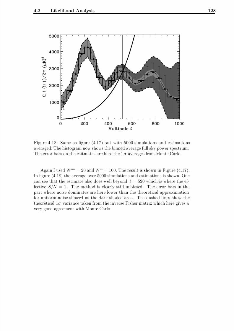
8/3/2019 Frode Kristian Hansen- Data Analysis of the Cosmic Microwave Background
http://slidepdf.com/reader/full/frode-kristian-hansen-data-analysis-of-the-cosmic-microwave-background 136/216
4.2 Likelihood Analysis 128
Figure 4.18: Same as figure (4.17) but with 5000 simulations and estimationsaveraged. The histogram now shows the binned average full sky power spectrum.The error bars on the esitmates are here the 1σ averages from Monte Carlo.
Again I used N bin = 20 and N in = 100. The result is shown in Figure (4.17).
In figure (4.18) the average over 5000 simulations and estimations is shown. Onecan see that the estimate also does well beyond = 520 which is where the ef-fective S/N = 1. The method is clearly still unbiased. The error bars in thepart where noise dominates are here lower than the theoretical approximationfor uniform noise showed as the dark shaded area. The dashed lines show thetheoretical 1σ variance taken from the inverse Fisher matrix which here gives avery good agreement with Monte Carlo.

8/3/2019 Frode Kristian Hansen- Data Analysis of the Cosmic Microwave Background
http://slidepdf.com/reader/full/frode-kristian-hansen-data-analysis-of-the-cosmic-microwave-background 137/216
4.2 Likelihood Analysis 129
Figure 4.19: The average correlation matrix N (b, b) ≡< DbDb > /(< Db ><Db >) − 1 of the estimates in figure (4.18). The negative elements are brightcoloured.
In figure (4.19) I show the average (over 5000 estimations) of the correla-
tion between the estimates Db between different bins. The figure shows that thecorrelations between estimates are low and in fact in each line all off-diagonalelements are more than an order of magnitude lower than the diagonal elementof that line. In Figure (4.20) I show that the probability distribution of the esti-mates in Figure (4.18) are almost Gaussian distributed.

8/3/2019 Frode Kristian Hansen- Data Analysis of the Cosmic Microwave Background
http://slidepdf.com/reader/full/frode-kristian-hansen-data-analysis-of-the-cosmic-microwave-background 138/216
4.2 Likelihood Analysis 130
Figure 4.20: The probability distribution of the estimates Db in figure 4.18. The
variable x is given as x = (Db
−< Db >)/ < (Db
−< Db >)2 >. The dashed
line is a Gaussian with mean and standard deviation taken from Monte-Carlo.The plot shows bin estimates centered at = 225, = 425, = 525 and = 725.
To test the method at higher multipoles I also did one estimation up to mul-tipole = 2048. I used HEALPix resolution N side = 1024 and simulated a skywith a 8 Gaussian beam and added non-uniform noise. Both the beam and noiselevel were adjusted according to the specifications for the Planck HFI 143GHzdetector (Bersanelli et al. 1996). I used again a 15 FWHM Gaussian Gaborwindow cut at 3σ away from the centre. In the estimation I used N bin = 40 bins
and N in
= 200 input C between = 7 and = 2048. The average of 100 suchsimulations is shown in figure (4.21). Each complete likelihood estimation (whichincludes a total of about 25 likelihood evaluations) took about 8 minutes on asingle processor on a 500MHz DEC Alpha work station.

8/3/2019 Frode Kristian Hansen- Data Analysis of the Cosmic Microwave Background
http://slidepdf.com/reader/full/frode-kristian-hansen-data-analysis-of-the-cosmic-microwave-background 139/216
4.2 Likelihood Analysis 131
Figure 4.21: Same as figure (4.14) for 100 simulations where the beam and noiselevel was set according to the specifications of the Planck 143GHz channel. Againa 15 FWHM Gaussian Gabor window was used. The power spectrum was esti-mated in 40 bins between = 2 and = 2048

8/3/2019 Frode Kristian Hansen- Data Analysis of the Cosmic Microwave Background
http://slidepdf.com/reader/full/frode-kristian-hansen-data-analysis-of-the-cosmic-microwave-background 140/216
4.2 Likelihood Analysis 132
Figure 4.22: The average of 300 estimations where the input C were taken fromsimulations with a fixed CMB realisation but varying noise realisations. Thedotted line is the N in input C from the CMB realisation without noise. Thehistogram is the same spectrum binned in N bin bins. The dashed line is thebinned average full sky power spectrum from which this realisation was made.The shaded areas around the binned full sky spectrum show the variance with
(dark) and without (bright) noise. The solid line rising from the left to the rightis the noise power spectrum.
In Figure (4.22), I have plotted the average of 300 estimations. The datainput in these 300 estimations were the C from simulations with a fixed CMBrealisation and varying noise realisation. The dotted line shows the N in C s usedas input to the likelihood but without the noise. The histogram is as before, theinput pseudo spectrum without noise binned in N bin bins. This means that eachhistogram line shows the average of the dotted line over the bin. One can see
that the result is partly following the N in
input˜
C and partly the binned powerspectrum.Finally, I made a comparison between a tophat window and a Gaussian Gabor
window. In this case I used uniform noise, so that the Gaussian and tophatGabor windows have the same S/N ratio which I set to 1 at = 520. I used a

8/3/2019 Frode Kristian Hansen- Data Analysis of the Cosmic Microwave Background
http://slidepdf.com/reader/full/frode-kristian-hansen-data-analysis-of-the-cosmic-microwave-background 141/216
4.2 Likelihood Analysis 133
disc with 18 radius, N in = 200 and N bin = 20. In Figure (4.23) one can seethe result. The lower plot shows the estimates with the Gaussian Gabor window(15 FWHM) and the upper with the tophat window. The Gaussian window issuppressing parts of the data and for this reason gets a higher sample variancethan the tophat. This effect is seen in the plot. Clearly when no noise weightingis required the tophat window seems to be the preferred window (which was
also discussed in (Hivon et al. 2001)). This chapter has been concentrating onthe Gaussian window to study power spectrum estimation in the presence of awindow different from a tophat. It has been shown that a different window canbe advantageous when the noise is not uniformly distributed as one can then givedata with different quality different significance.

8/3/2019 Frode Kristian Hansen- Data Analysis of the Cosmic Microwave Background
http://slidepdf.com/reader/full/frode-kristian-hansen-data-analysis-of-the-cosmic-microwave-background 142/216
4.3 Extensions of the Method 134
Figure 4.23: Estimates of C using a Gaussian Gabor window (lower plot) and atophat window (upper plot). Here I used a uniform noise model with S/N = 1
at = 520. The dotted line shows the average full sky power spectrum andthe histogram shows the input pseudo power spectrum without noise for thisrealisation, binned in the same way as the estimates. The bright shaded areashows the cosmic and sample variance around the binned average spectrum (notplotted). The dark shaded area has the variance due to noise included. The 1σerror bars on the estimates are taked from the inverse Fisher matrix. The solidline increasing from left to right is the noise power spectrum.
4.3 Extensions of the Method
In this section I will discuss two possible extensions of the method. The for-malism for the extensions are worked out and some simple examples are shown.Further investigations of these extensions are left for future work.
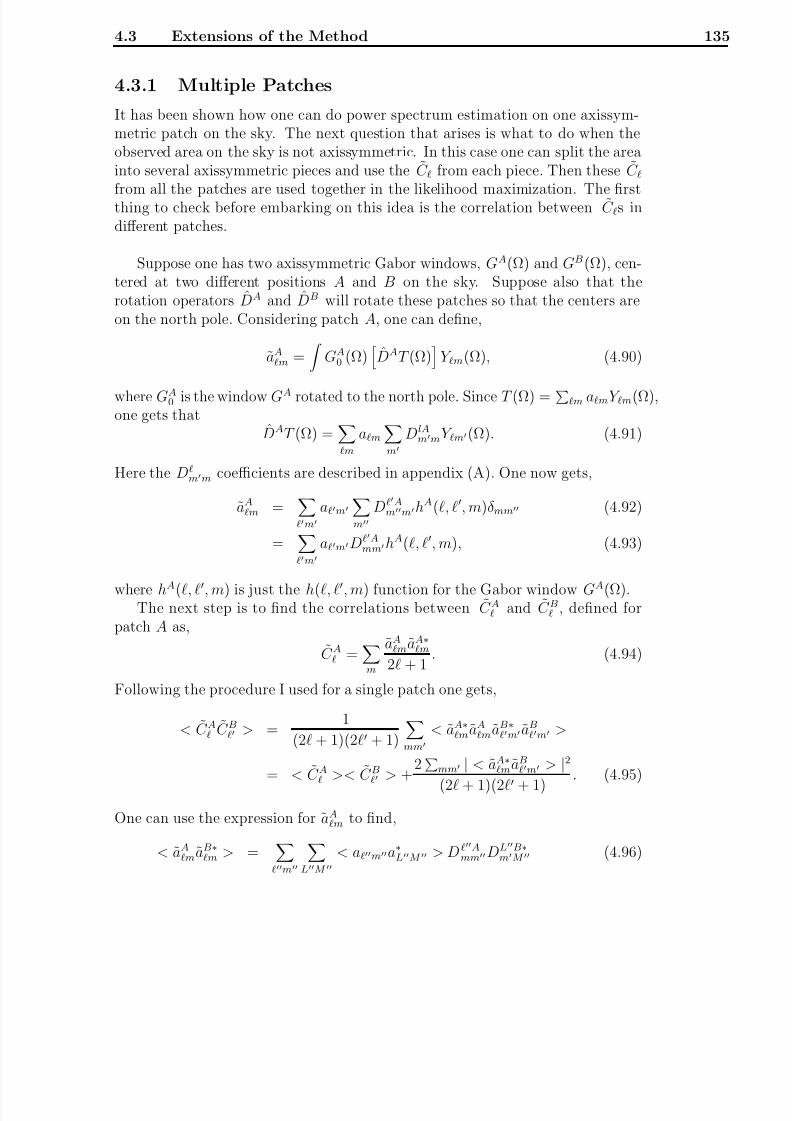
8/3/2019 Frode Kristian Hansen- Data Analysis of the Cosmic Microwave Background
http://slidepdf.com/reader/full/frode-kristian-hansen-data-analysis-of-the-cosmic-microwave-background 143/216
4.3 Extensions of the Method 135
4.3.1 Multiple Patches
It has been shown how one can do power spectrum estimation on one axissym-metric patch on the sky. The next question that arises is what to do when theobserved area on the sky is not axissymmetric. In this case one can split the areainto several axissymmetric pieces and use the C from each piece. Then these C
from all the patches are used together in the likelihood maximization. The firstthing to check before embarking on this idea is the correlation between C s indifferent patches.
Suppose one has two axissymmetric Gabor windows, GA(Ω) and GB(Ω), cen-tered at two different positions A and B on the sky. Suppose also that therotation operators DA and DB will rotate these patches so that the centers areon the north pole. Considering patch A, one can define,
aAm =
GA0 (Ω)
DAT (Ω)
Y m(Ω), (4.90)
where GA0 is the window GA rotated to the north pole. Since T (Ω) = m amY m(Ω),
one gets thatDAT (Ω) =
m
am
m
DlAmmY m(Ω). (4.91)
Here the Dmm coefficients are described in appendix (A). One now gets,
aAm =
m
am
m
DAmmhA(, , m)δmm (4.92)
=m
amDAmmhA(, , m), (4.93)
where hA(, , m) is just the h(, , m) function for the Gabor window GA(Ω).The next step is to find the correlations between C A and C B , defined for
patch A as,
C A =
m
aAmaA∗
m
2 + 1. (4.94)
Following the procedure I used for a single patch one gets,
< C A C B > =1
(2 + 1)(2 + 1)
mm
< aA∗maA
maB∗m aB
m >
= < C A >< C B > +2mm | < aA∗
maBm > |2
(2 + 1)(2 + 1). (4.95)
One can use the expression for aAm to find,
< aAmaB∗
m > =
m
LM
< ama∗LM > DAmmDLB∗
mM (4.96)

8/3/2019 Frode Kristian Hansen- Data Analysis of the Cosmic Microwave Background
http://slidepdf.com/reader/full/frode-kristian-hansen-data-analysis-of-the-cosmic-microwave-background 144/216
4.3 Extensions of the Method 136
× hA(, , m)hB(, L, m) (4.97)
=
C
m
DAmmDB∗
mm
D
mm (∆)
hA(, , m)hB(, , m) (4.98)
= C d
mm(∆)hA(, , m)hB(, , m), (4.99)
where ∆ is the angel between the centers of the patches. Relations from appendix(A) were used here.
The next step is to see what happens when noise is introduced. I assume thatthe noise is uncorrelated. The noise in pixel j is n j and < n j n j >= δ jj σ
2 j . From
above one has,C A = C AS
+ C AN + C AX
, (4.100)
where
C AN
=
m
aNAm aN A∗
m
2 + 1(4.101)
C AX =
m
aNAm aSA∗
m
2 + 1(4.102)
aAN m =
j
GA j nA
j Y jm, (4.103)
where the last sum is over pixels, GA j and nA
j being the window and noise forpixel j respectively.
The correlation between the two patches then becomes,
< C A
C B
>
−< C A
>< C B
>= M S
+ M N
+ < C AX
C BX
>, (4.104)
where,
M S =
2
(2 + 1)(2 + 1)
mm
| < aAS ∗m aBS
m > |2 (4.105)
M N =
2
(2 + 1)(2 + 1)
mm
| < aAN ∗m aBN
m > |2. (4.106)
Finally,
< C AX
C BX
>=
4
(2 + 1)(2 + 1) mm
< aAS ∗
m
aBS
m >< aAN ∗
m
aBN
m > . (4.107)
Now one needs an expression for < aAN m aBN ∗
m >. One gets,
< aAN m aBN ∗
m >= jj
GA j GB
j < nA j nB
j > Y jmY j
m. (4.108)

8/3/2019 Frode Kristian Hansen- Data Analysis of the Cosmic Microwave Background
http://slidepdf.com/reader/full/frode-kristian-hansen-data-analysis-of-the-cosmic-microwave-background 145/216
4.3 Extensions of the Method 137
Here there are only correlations between overlapping pixels. If there are no over-lapping pixels between the patches, this term is zero. Otherwise this can bewritten as a sum over the overlapping pixels
< aAN m aBN ∗
m >=
j
GA j GB
j σ2 j Y jmY j
m. (4.109)
After the expression (4.95) was tested with Monte Carlo simulations, I com-puted the correlations between C for two patches A and B where I varied thedistance θ between the centers of A and B. I used a standard CDM power spec-trum and both patches A and B had a radius of 18 apodised with a 15 FWHMGaussian Gabor window. In figure (4.24) I have plotted the diagonal of the nor-malised correlation matrix (< C A C B > − < C >2)/ < C >2. The angels θ Iused were 6, 12, 24, 30, 36 and 180. One sees clearly how the correlationsdrop with the distance. In the two last cases, there were no common pixels inthe patches. As one could expect, the correlations for the largest angels (the firstfew multipoles) do not drop that fast.

8/3/2019 Frode Kristian Hansen- Data Analysis of the Cosmic Microwave Background
http://slidepdf.com/reader/full/frode-kristian-hansen-data-analysis-of-the-cosmic-microwave-background 146/216
4.3 Extensions of the Method 138
Figure 4.24: The correlation between C between two patches A and B with anangular distance θ between the centers. A normal CDM power spectrum was usedand the patches had an 18 radius apodised with a 15 FWHM Gaussian Gaborwindow. The figure shows the diagonal of the normalised correlation matrix(< C A C B > − < C >2)/ < C >2 where of course < C >=< C A >=< C B >The angles used are (from top to bottom on the figure) 0, 6, 12, 18, 30, 36
and 180.
In figure (4.25) I have plotted two slices through the correlation matrix of C for a single patch at = 400 and = 800. On the top I plotted the diagonalsof the correlation matrices for separation angle θ = 30, θ = 36 and θ = 180.One sees that for the case where the patches do not have overlapping pixels, thewhole diagonals have the same level as the far-off-diagonal elements in the θ = 0
matrix. When doing power spectrum estimation on one patch, the result did notchange significantly when these far-off-diagonal elements were set to zero. Forthis reason one expects that when analysing several patches which do not overlapsimultaneously, the correlations between non-overlapping patches do not need tobe taken into account. Note however that for the θ = 30 which means that thereare only a few overlapping pixels, the approximation will not be that good as thelevel is orders of magnitude above the far-off-diagonals of the θ = 0 matrix.Another thing to note is that for the lowest multipoles, the correlation between

8/3/2019 Frode Kristian Hansen- Data Analysis of the Cosmic Microwave Background
http://slidepdf.com/reader/full/frode-kristian-hansen-data-analysis-of-the-cosmic-microwave-background 147/216
4.3 Extensions of the Method 139
patches is still high but I will also assume this part to be zero and attempt a joint analysis of non-overlapping patches.
Figure 4.25: Cuts through the correlation matrices which diagonals are shownin figure (4.24). The solid lines (thin and thick) show a cut through the θ = 0
correlation matrix at = 400 and = 800 respectively. The dashed lines (thin
and thick) show the diagonal of the correlation matrices for θ = 36 and θ = 30
respectively. The dotted line is the diagonal of the θ = 180 matrix.
The full correlation matrices for 0 and 30 degree separation are shown infigure (4.26). The figures show how the diagonal is dropping relative to the faroff-diagonal elements.
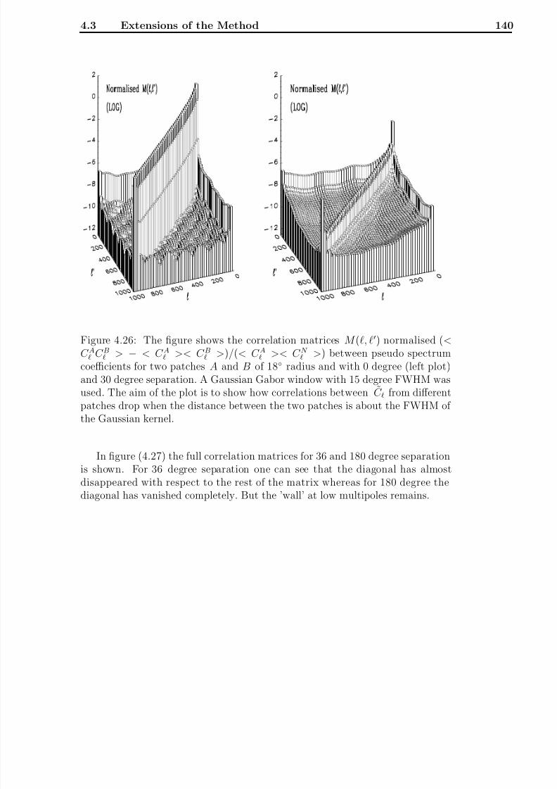
8/3/2019 Frode Kristian Hansen- Data Analysis of the Cosmic Microwave Background
http://slidepdf.com/reader/full/frode-kristian-hansen-data-analysis-of-the-cosmic-microwave-background 148/216
4.3 Extensions of the Method 140
Figure 4.26: The figure shows the correlation matrices M (, ) normalised (<C A C B > − < C A >< C B >)/(< C A >< C N
>) between pseudo spectrumcoefficients for two patches A and B of 18 radius and with 0 degree (left plot)and 30 degree separation. A Gaussian Gabor window with 15 degree FWHM wasused. The aim of the plot is to show how correlations between C from differentpatches drop when the distance between the two patches is about the FWHM of
the Gaussian kernel.
In figure (4.27) the full correlation matrices for 36 and 180 degree separationis shown. For 36 degree separation one can see that the diagonal has almostdisappeared with respect to the rest of the matrix whereas for 180 degree thediagonal has vanished completely. But the ’wall’ at low multipoles remains.

8/3/2019 Frode Kristian Hansen- Data Analysis of the Cosmic Microwave Background
http://slidepdf.com/reader/full/frode-kristian-hansen-data-analysis-of-the-cosmic-microwave-background 149/216
4.3 Extensions of the Method 141
Figure 4.27: This figure shows the same as figure (4.26) but for 36 and 180 degreeseparation of the patches.
In figure (4.28), I did a separate C estimation on 146 non-overlapping patcheswith radius 18 apodised with a 15 FWHM Gaussian Gabor window. Thepatches where uniformly distributed over the sphere and and uniform noise wasadded to the whole map. The figure shows the average of the 146 C estimates.One can see that the estimate seems to be approaching the full sky power spec-trum even at small multipoles.

8/3/2019 Frode Kristian Hansen- Data Analysis of the Cosmic Microwave Background
http://slidepdf.com/reader/full/frode-kristian-hansen-data-analysis-of-the-cosmic-microwave-background 150/216
4.3 Extensions of the Method 142
Figure 4.28: The average of 146 individual power spectrum estimations of 146non-overlapping patches on the same CMB map with uniform noise added to it.The patches all had radius 18 degrees apodised with a 15 FWHM GaussianGabor window. The histogram shows the binned average of the 146 C from thedifferent patches without noise. The dotted line is the average full sky powerspectrum and the shaded areas around the binned full sky power spectrum (not
plotted) show the theoretical 1σ variance with (dark) and without (bright) noise.The solid line rising from the left to the right is the noise power spectrum.

8/3/2019 Frode Kristian Hansen- Data Analysis of the Cosmic Microwave Background
http://slidepdf.com/reader/full/frode-kristian-hansen-data-analysis-of-the-cosmic-microwave-background 151/216
4.3 Extensions of the Method 143
Figure 4.29: The result of a joint analysis of 146 patches on the same CMB sky.The solid line shows the average full sky power spectrum, the histogram showsthe binned full sky power spectrum and the shaded boxes show the expected 2σdeviations due to noise, cosmic and sample variance. The sizes of the shadedboxes were calculated from the approximate formula for uniform noise. The dotsshow the estimates with 2σ error bars taken from the Fisher matrix. As before
the rising solid line is the noise power spectrum and the vertical line shows whereS/N = 1.
Finally I made a joint analysis of all the 146 patches. The idea was to extendthe datavector in the likelihood so that it contained all the C from all the 146patches. The datavector can then be written as d = d1, d2, ..., d146 where di
now denotes the whole datavector for patch number i. From the results aboveit seems to be a good approximation to assume that the correlation betweenC from different patches is zero so that the correlation matrix will be block
diagonal. Each block is then the correlation matrix for each individual patch.The log-likelihood can then simply be written as
L =146i=1
dT i M−1
i di +146i=1
ln det Mi, (4.110)

8/3/2019 Frode Kristian Hansen- Data Analysis of the Cosmic Microwave Background
http://slidepdf.com/reader/full/frode-kristian-hansen-data-analysis-of-the-cosmic-microwave-background 152/216
4.3 Extensions of the Method 144
where Mi is the correlation matrix for patch number i. In figure (4.29) the resultof this joint analysis is shown. One can see that the full sky power spectrum iswell within the two sigma error bars of the estimates.
The method of combining patches on the sky for power spectrum analysis willbe developed further in a forthcoming paper (Gorski and Hansen 2002).
4.3.2 Monte Carlo Simulations of the Noise Correlations
and Extention to Correlated Noise
The computation of the noise correlation matrix in the general case takes
N pixl2max(N in)2
which is approximately N 3/2
pix (N in)2. When N in is getting large this can be cal-culated quicker using Monte Carlo simulations (as was done in (Hivon et al.
2001)). Finding the C N from one noise map takes O(N
3/2 pix ) operations so using
Monte Carlo simulations to find the whole noise matrix takes O(N 3/2
pix N sim) op-eration where N sim is the number of Monte Carlo simulations needed. So when
N sim << (N 2in) it will be advantageous using MC if this gives the same result.
Also when the noise gets correlated, the analytic calculation of < aN maN
m >will be very expensive. In this case another method for computing < amam >will be necessary and Monte Carlo simulations could also prove useful. For agiven noise model several noise realisations can be made and averaged to yieldthe noise correlation matrix and the < amam > term needed in the estimationprocess. Using Monte Carlo the operations count for precalculations of noiseproperties will still be O(N
3/2 pix ) also with correlated noise assuming that each
noise realisation for a given noise model can be calculated quickly.
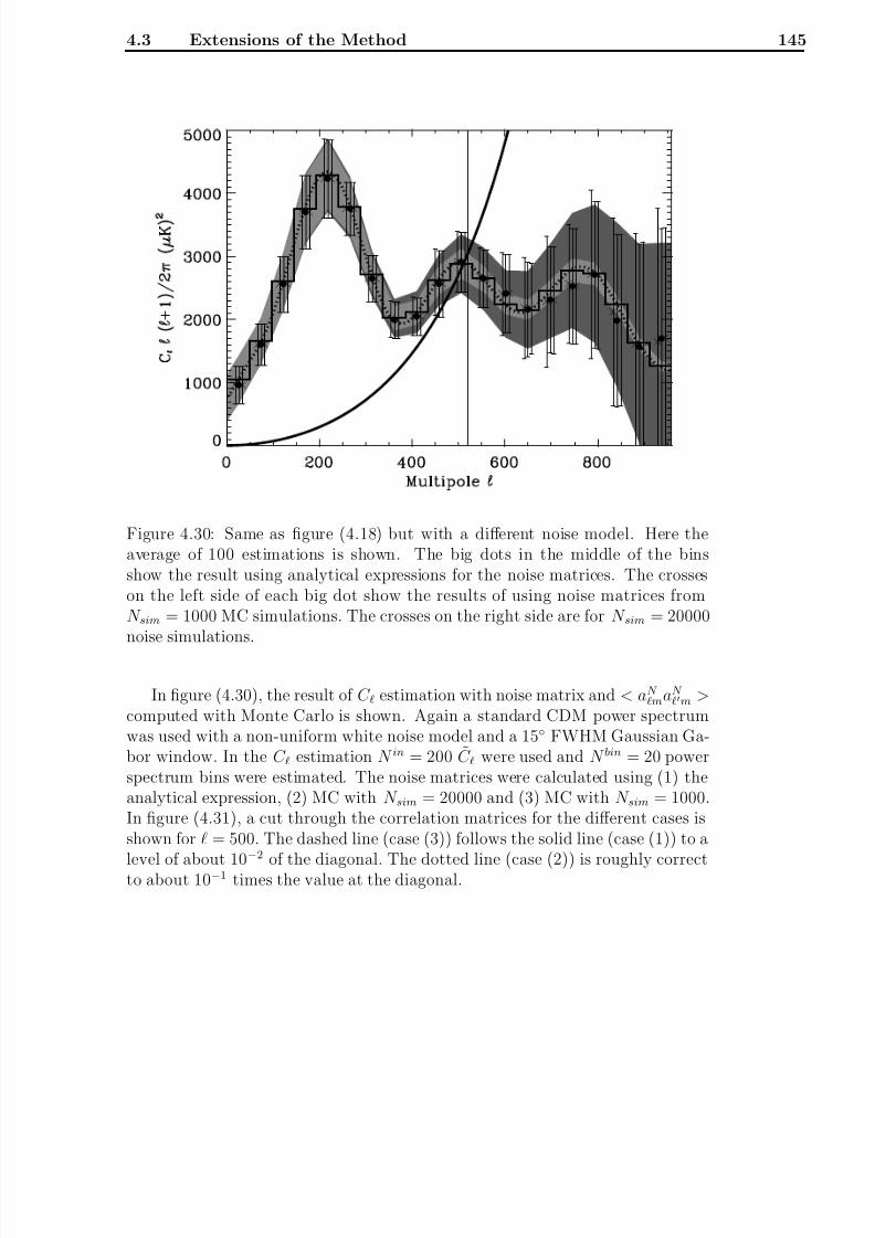
8/3/2019 Frode Kristian Hansen- Data Analysis of the Cosmic Microwave Background
http://slidepdf.com/reader/full/frode-kristian-hansen-data-analysis-of-the-cosmic-microwave-background 153/216
4.3 Extensions of the Method 145
Figure 4.30: Same as figure (4.18) but with a different noise model. Here theaverage of 100 estimations is shown. The big dots in the middle of the binsshow the result using analytical expressions for the noise matrices. The crosseson the left side of each big dot show the results of using noise matrices fromN sim = 1000 MC simulations. The crosses on the right side are for N sim = 20000noise simulations.
In figure (4.30), the result of C estimation with noise matrix and < aN maN
m >computed with Monte Carlo is shown. Again a standard CDM power spectrumwas used with a non-uniform white noise model and a 15 FWHM Gaussian Ga-bor window. In the C estimation N in = 200 C were used and N bin = 20 powerspectrum bins were estimated. The noise matrices were calculated using (1) theanalytical expression, (2) MC with N sim = 20000 and (3) MC with N sim = 1000.In figure (4.31), a cut through the correlation matrices for the different cases isshown for = 500. The dashed line (case (3)) follows the solid line (case (1)) to a
level of about 10
−2
of the diagonal. The dotted line (case (2)) is roughly correctto about 10−1 times the value at the diagonal.

8/3/2019 Frode Kristian Hansen- Data Analysis of the Cosmic Microwave Background
http://slidepdf.com/reader/full/frode-kristian-hansen-data-analysis-of-the-cosmic-microwave-background 154/216
4.3 Extensions of the Method 146
Figure 4.31: A cut through the noise correlation matrix at multipole = 500.The correlation matrix was evaluated using the analytical formulae (solid line),20000 MC simulations (dashed line) and 1000 MC simulations (dotted line). Thematrix is here normalised to be 1 at the diagonal.
I did 100 estimations for each case and the average result is plotted in figure(4.30). The big dots are the results from case (1), the crosses on the right handside are the results from (2) and the crosses on the left hand side the resultsfrom (3). The average estimates seem to be consistent, only in the highly noisedominated regime they start to deviate. For case (2), the error bars are for somemultipoles higher and for some lower than the analytic case. The differencesare at most 3%. I conclude that using this many simulations, the error bars donot increase significantly over the analytic case. For case (3) the error bars areup to 17% higher (and only higher) than the analytic case. It seems that 1000simulations was not sufficient to keep the same accuracy of the estimates as when
using analytic noise matrices. To keep the error bars as low as possible it seemsthat N sim = 20000 is a reasonable number of simulations.

8/3/2019 Frode Kristian Hansen- Data Analysis of the Cosmic Microwave Background
http://slidepdf.com/reader/full/frode-kristian-hansen-data-analysis-of-the-cosmic-microwave-background 155/216
4.4 Discussion 147
4.4 Discussion
In this chapter I have discussed the Gabor transform on the sphere and how thiscan be used for CMB power spectrum estimation. A powerful tool has been pre-sented for estimation of the full sky CMB power spectrum using small patches onthe sky. The method is very fast an gives an unbiased estimate for the multipoles
for which the Gaussian likelihood ansatz is valid. For the lowest multipoles asmall downwards biasing is observed for small windows due to the skewed distri-bution of C . This can easily be solved by using information about low multipoleC from larger patches. When estimating the power spectrum for larger parts of the sky this small bias disappears.
The method has been demonstrated to work very well on a single azimuthallysymmetric patch on the CMB sky. It was also shown how the method can beextended to non-symmetric patches or even full sky by combining several patchesin a joint likelihood analysis. This was only tested for the uniform noise case butwill be explored further in future work. Also the case with correlated noise should
in principle work using Monte Carlo methods to precompute noise matrices. Thiswas tested for uncorrelated noise and compared to the analytic precalculationscheme. The results were getting more and more similar as the number of MonteCarlo simulations was increased. This is another extension which needs morework in the future.

8/3/2019 Frode Kristian Hansen- Data Analysis of the Cosmic Microwave Background
http://slidepdf.com/reader/full/frode-kristian-hansen-data-analysis-of-the-cosmic-microwave-background 156/216
4.4 Discussion 148
8/3/2019 Frode Kristian Hansen- Data Analysis of the Cosmic Microwave Background
http://slidepdf.com/reader/full/frode-kristian-hansen-data-analysis-of-the-cosmic-microwave-background 157/216
Chapter 5
Gabor Transform on the
Polarised CMB Sky
As discussed in chapter (1) and (2) the observation of the CMB polarisationpower spectra will help breaking some parameter degeneracies. Several different
sets of values for the cosmological parameters can give the same CMB temper-ature power spectrum. The polarisation power spectra will however be differentand can distinguish the different models. Also the error bars on the cosmologicalparameters can be reduced by also exploiting the information present in the CMBpolarisation power spectra.
Much effort has been made recently in order to find methods to analyse theCMB temperature power spectrum. For the even harder task of estimating thepolarisation power spectra there has been very few publications. The frameworkfor analysing the polarisation power spectra has been set in (Zaldarriaga and
Seljak 1997; Kamionkowski, Kosowsky, and Stebbins 1997) but these papers onlydescribe the full likelihood method which is far too time consuming also whenonly considering the temperature power spectrum.
In this chapter I will extend the method of using the pseudo power spectrumas input to a likelihood estimation of the power spectrum. I will include the E and C mode polarisation pseudo power spectra in the datavector and use tech-niques similar to those described in the previous chapter to estimate the powerspectra. This can be done because the kernels that connect the full sky polari-sation power spectra with the polarisation pseudo power spectra on an apodisedsky are similar to the kernel for the temperature power spectrum. In the first part
of this chapter I will derive the formulae for these kernels and for the polarisationpseudo power spectra and discuss their shapes. Then in the second part this willbe used for likelihood estimation.
In this chapter the B component polarisation will mostly be neglected. The

8/3/2019 Frode Kristian Hansen- Data Analysis of the Cosmic Microwave Background
http://slidepdf.com/reader/full/frode-kristian-hansen-data-analysis-of-the-cosmic-microwave-background 158/216
5.1 The Gabor Transformation 150
B polarisation power spectrum is expected to be very small and will hardly bedetectable by the MAP or Planck experiments. Also the E and B componentsof polarisation mixes on the cut sky as will be discussed in this chapter, makingthe B polarisation pseudo spectrum to be dominated by the E component. Thiswas also found independently by (Lewis, Challinor, and Turok 2001; Chiueh andMa 2001).
5.1 The Gabor Transformation
5.1.1 Polarisation Powerspectra
As described in the first chapter the polarisation spherical harmonic coefficientsare defined by means of the tensor spherical harmonics 2Y m(n) as
a2,m =
dn 2Y ∗m(n)(Q + iU )(n), (5.1)
a−2,m = dn −2Y ∗m(n)(Q
−iU )(n), (5.2)
and the inverse transforms are given as
(Q + iU )(n) =m
a2,m 2Y m(n) (5.3)
(Q − iU )(n) =m
a−2,m −2Y m(n). (5.4)
It will be advantageous to write these spherical harmonics in terms of the rotationmatrices D
mm defined in Appendix (A). Using the formulae in Appendix (B)one can write
2Y m(n) = 2 + 1
4π
D−2m(φ,θ, 0), (5.5)
−2Y m(n) =
2 + 1
4πD
2m(φ,θ, 0). (5.6)
(5.7)
The corresponding complex conjugates can be written as (using the relations inAppendix (A))
2Y ∗m(n) =
2 + 1
4πD∗−2m(φ,θ, 0) (5.8)
= 2 + 1
4π(
−1)mD
2−m(φ,θ, 0), (5.9)
−2Y ∗m(n) =
2 + 1
4πD∗
2m(φ,θ, 0) (5.10)
=
2 + 1
4π(−1)mD
−2−m(φ,θ, 0). (5.11)

8/3/2019 Frode Kristian Hansen- Data Analysis of the Cosmic Microwave Background
http://slidepdf.com/reader/full/frode-kristian-hansen-data-analysis-of-the-cosmic-microwave-background 159/216
5.1 The Gabor Transformation 151
Finally as explained in chapter (1) the power spectrum can be written in termsof a ‘divergence free’ E component and a ‘curl free’ B component
aE,m = −1
2(a2,m + a−2,m), (5.12)
aB,m =1
2i(a2,m − a−2,m) (5.13)
Now I will define the windowed coefficients am and C for polarisation inan analogous way as for temperature. As in chapter (4) I Legendre expand theGabor Window G(θ) which is an axissymmetric function centered at n0,
G(θ) =
2 + 1
4πgP (cos θ) =
m
gY m(n)Y ∗m(n0). (5.14)
=
m
g
2 + 1
4πD
0m(φ,θ, 0)Y m(n0). (5.15)
I define the windowed coefficients am as
a2,m =
dn 2Y ∗m(n)(Q + iU )(n)G(n, n0) (5.16)
Using the expression for (5.3) (Q + iU )(n) and writing all 2Y m as D-matricesusing expressions (5.5), (5.6), (5.9) and (5.11) one gets,
a2,m =m
a2,m
m
g
(2 + 1)(2 + 1)(2 + 1)
(4π)3/2(−1)m (5.17)
×Y
m(n
0) dnD
−2m(φ,θ, 0)D
2−m(φ,θ, 0)D
0m(φ,θ, 0) (5.18)
=m
a2,m
m
g
(2 + 1)(2 + 1)(2 + 1)
(4π)3/2(−1)m 1
2π(5.19)
× Y m(n0)
dndγD
−2m(φ,θ,γ )D2−m(φ,θ,γ )D
0m(φ,θ,γ ) (5.20)
=m
a2,mh2(, , m , m, n0). (5.21)
By using equation (5.16), one can also write this as,
a2,n = m
a2,m dnG(n, n0) 2Y ∗m(n) 2Y m(n). (5.22)
Using the two last expressions, the h2 function can be written in two ways(using relation (C.2) for the last expression),
h2(, , m , m, n0) ≡
dnG(n, n0) 2Y ∗m(n) 2Y m(n) (5.23)

8/3/2019 Frode Kristian Hansen- Data Analysis of the Cosmic Microwave Background
http://slidepdf.com/reader/full/frode-kristian-hansen-data-analysis-of-the-cosmic-microwave-background 160/216
5.1 The Gabor Transformation 152
=
m
g
(2 + 1)(2 + 1)(2 + 1)
4π(−1)m (5.24)
× Y m(n0)
−2 2 0
m −m m
. (5.25)
As I soon will show, the polarisation pseudo power spectra are rotationallyinvariant under rotation of the Gabor window. For that reason, one can put thecentre of the Gabor window on the north pole giving,
a2,m =
a2,mh2(, , m), (5.26)
where,
h2(, , m) = h2(, ,m,m, 0) (5.27)
= g
(2 + 1)(2 + 1)(2 + 1)
4π(5.28)
× (−1)m
−2 2 0
m −m 0
. (5.29)
Similarly one gets,
a−2,m =
a−2,mh2(, , −m) (5.30)
and
aE,m =
−1
2
(a2,m + a−2,m) (5.31)
=
aE,mH 2(, , m) + i
aB,mH −2(, , m) (5.32)
aB,m = i1
2(a2,m − a−2,m) (5.33)
=
aB,mH 2(, , m) − i
aE,mH −2(, , m) (5.34)
Please note that whereas h(, , −m) = h(, , m) a similar relation does notexist for h2(, , −m). Using the expression above, one has that,
h2(, , −m) =
g
(2 + 1)(2 + 1)(2 + 1)
4π(−1)m (5.35)
×
−2 2 0
m −m 0
(−1)++ (5.36)

8/3/2019 Frode Kristian Hansen- Data Analysis of the Cosmic Microwave Background
http://slidepdf.com/reader/full/frode-kristian-hansen-data-analysis-of-the-cosmic-microwave-background 161/216
5.1 The Gabor Transformation 153
The reason why this is not equal to h2(, , m) is that the first Wigner symbolis not zero when + + is even, which is the case when the whole lower rowin the Wigner symbol is 0, as in the case with h(, , m). It is also obvious fromthe expression (5.22). For the scalar case, the relation Y (−m)(n) = (−1)mY m(n)ensures that there is no dependency on m in h(, , m) whereas a similar relationdoes not exist for the tensor harmonics (but see relation (B.5)).
I have further defined,
H 2(, , m) =1
2(h2(, , m) + h2(, , −m)) (5.37)
H −2(, , m) =1
2(h2(, , m) − h2(, , −m)) (5.38)
which contrary to h2(, , m) have an m-symmetry
H 2(, , −m) = H 2(, , m) (5.39)
H −2(,
, −m) = −H −2(,
, m) (5.40)
To find the C and (later) the correlation matrices, the following quantitieswill be needed
< aE,ma∗E,,m > = δmm
C E H 2(, , m)H 2(, , m) (5.41)
+
C BH −2(, , m)H −2(, , m)
(5.42)
< aB,ma∗B,,m > = δmm
C BH 2(, , m)H 2(, , m) (5.43)
+
C E H −2(, , m)H −2(, , m)
(5.44)
< aE,ma∗B,,m > = δmmi
C E
H 2(, , m)H −2(, , m) (5.45)
+
C BH −2(, , m)H 2(, , m)
(5.46)
< aE,ma∗,m > = δmm
C C H 2(, , m)h(, , m) (5.47)
< aB,ma∗,m > = −iδmm
C C H −2(, , m)h(, , m) (5.48)
For < C E > one now has,
< C E >=
m
< a∗E,maE,m >
2 + 1=
C E
K 2(, ) +
C B K −2(, ). (5.49)

8/3/2019 Frode Kristian Hansen- Data Analysis of the Cosmic Microwave Background
http://slidepdf.com/reader/full/frode-kristian-hansen-data-analysis-of-the-cosmic-microwave-background 162/216
5.1 The Gabor Transformation 154
Where,
K ±2(, ) =1
2 + 1
m
H 2±2(, , m) (5.50)
Using the expression for h2(, , m), one gets
K ±2(,
) =
1
2
1
2 + 1 mh
2
2(,
, m) ± h2(,
, m)h2(,
, −m) (5.51)
=
L
ggL
(2 + 1)(2 + 1)(2L + 1)
32π2(5.52)
×
−2 2 0
L
−2 2 0
(1 ± (−1)++) (5.53)
× m
m −m 0
L
m −m 0
(2+1)−1δL
(5.54)
= g
2
(2 + 1)(2 + 1)
32π2
−2 2 0 2
(5.55)
× (1 ± (−1)++). (5.56)
Similarly,
< C B > =
C B K 2(, ) +
C E K −2(, ) (5.57)
< C C > =
C C K 20(, ) (5.58)
K 20(, ) =1
2 + 1 m H 2(, , m)h(, , m) (5.59)
=
g2(2 + 1)(2 + 1)
16π2
−2 2 0
0 0 0
. (5.60)
Before studying these kernels I will first show the rotational invariance. To showthat < C E
>, < C B > and < C C > are rotationally invariant under rotations of
the window, one can keeps the dependency on the angle and the expression forthe kernel turns out to be,
K ±2(, , n0) =1
2
1
2 + 1
mm
h22(, , m , m, n0) (5.61)
±h2(, , m , m, n0)h2(, , −m, −m, n0)
(5.62)
=
L
mM
ggL
(2 + 1)
(2 + 1)(2L + 1)
8π(5.63)

8/3/2019 Frode Kristian Hansen- Data Analysis of the Cosmic Microwave Background
http://slidepdf.com/reader/full/frode-kristian-hansen-data-analysis-of-the-cosmic-microwave-background 163/216
5.1 The Gabor Transformation 155
× Y m(n0)Y ∗LM (n0)
−2 2 0
L
−2 2 0
(5.64)
× mm
m −m m
L
m −m M
(2+1)−1δLδmM
(5.65)
× (1 ± (−1)+
+
) (5.66)
=
g22 + 1
8π
−2 2 0
2m
|Y m(n0)|2
2+14π
(5.67)
× (1 ± (−1)++) (5.68)
= K ±2(, ). (5.69)
This is independent on the angle n0 which shows the rotational invariance of thepseudo polarisation power spectra.
As with the temperature kernels, the polarisation kernels can be evaluatedeither using the analytical Wigner symbol expressions (5.55) and (5.58) or fasterby direct integration and recursion of the H ±2 functions. The recursion for theh2(, , m , m) functions in appendix (E) is one of the major results in the thesis.This is an extension of the recursion for h(, , m , m) in appendix (D).
Studying equation (5.49) and (5.57) one sees that the E and B modes aremixing when only a portion of the sky is observed. The kernel K 2(, ) is thekernel which takes full sky C E
modes to the pseudo coefficients C E and similarly
for C B . The kernel K −2(, ) is the one which causes the mixing. In figure (5.1)
and (5.2) I have plotted the kernels K 2(, ) together with K −2(, ) for a 5 and15 degree FWHM Gaussian Gabor window with θC = 3σ. One can see that thediagonal of the K 2(, ) kernel is about an order of magnitude larger than thediagonal of the mixing kernel K −2(, ). This means that C E
would dominateC E
and C B would dominate C B provided that the two spectra C E and C B were
of the same order of magnitude. However as discussed before, the C B are ex-pected to be considerably smaller than C E
in most cosmological models. For theE mode this is not a problem as C E
will then hardly be affected. The problemis the B mode which in this case will be dominated by the E mode.

8/3/2019 Frode Kristian Hansen- Data Analysis of the Cosmic Microwave Background
http://slidepdf.com/reader/full/frode-kristian-hansen-data-analysis-of-the-cosmic-microwave-background 164/216
5.1 The Gabor Transformation 156
Figure 5.1: The kernels K 2(, ) (left plot) and K −2(, ) (right plot) connectingfull and cut sky polarisation power spectra C E
and C B . The left kernel is theone which takes full sky C E
into cut sky C E and full sky C B into cut sky C B .
The right kernel is the one which mixes the two giving contributions from fullsky C E
in cut sky C B and vice versa.

8/3/2019 Frode Kristian Hansen- Data Analysis of the Cosmic Microwave Background
http://slidepdf.com/reader/full/frode-kristian-hansen-data-analysis-of-the-cosmic-microwave-background 165/216
5.1 The Gabor Transformation 157
Figure 5.2: The same as figure (5.1) for a 15 degree FWHM Gaussian Gaborwindow.
The separation of E and B modes of polarisation on the cut sky was alreadydiscussed in (Lewis, Challinor, and Turok 2001; Chiueh and Ma 2001). Here I
will only note that an easy way of separating the two would be to construct twonew coefficients
a+,m = aE,m + iaB,m (5.70)
a−,m = aE,m − iaB,m, (5.71)
with the corresponding pseudo quantities
a+,m =
a+,m(H 2(, , m) + H −2(, , m)) (5.72)
a−,m =
a−,m(H 2(, , m) − H −2(, , m)) (5.73)
(5.74)
For the power spectra one gets,
< C + > ≡ m
< a+,ma∗+,m >
2 + 1=< C E
m > + < C Bm >, (5.75)
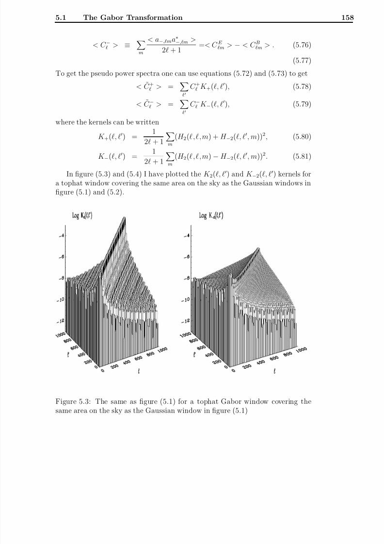
8/3/2019 Frode Kristian Hansen- Data Analysis of the Cosmic Microwave Background
http://slidepdf.com/reader/full/frode-kristian-hansen-data-analysis-of-the-cosmic-microwave-background 166/216
5.1 The Gabor Transformation 158
< C − > ≡ m
< a−,ma∗−,m >
2 + 1=< C E
m > − < C Bm > . (5.76)
(5.77)
To get the pseudo power spectra one can use equations (5.72) and (5.73) to get
< C + > =
C + K +(, ), (5.78)
< C − > =
C − K −(, ), (5.79)
where the kernels can be written
K +(, ) =1
2 + 1
m
(H 2(,,m) + H −2(, , m))2, (5.80)
K −(, ) =1
2 + 1
m
(H 2(,,m) − H −2(, , m))2. (5.81)
In figure (5.3) and (5.4) I have plotted the K 2(, ) and K −2(, ) kernels fora tophat window covering the same area on the sky as the Gaussian windows in
figure (5.1) and (5.2).
Figure 5.3: The same as figure (5.1) for a tophat Gabor window covering thesame area on the sky as the Gaussian window in figure (5.1)

8/3/2019 Frode Kristian Hansen- Data Analysis of the Cosmic Microwave Background
http://slidepdf.com/reader/full/frode-kristian-hansen-data-analysis-of-the-cosmic-microwave-background 167/216
5.1 The Gabor Transformation 159
Figure 5.4: The same as figure (5.2) for a tophat Gabor window covering thesame area on the sky as the Gaussian window in figure (5.2)
The kernel K 20(, ) for the cross polarisation power spectrum C C is shown
in figure (5.5) for a 5 and 15 degree Gaussian window and in figure (5.6) for thecorresponding tophat windows.
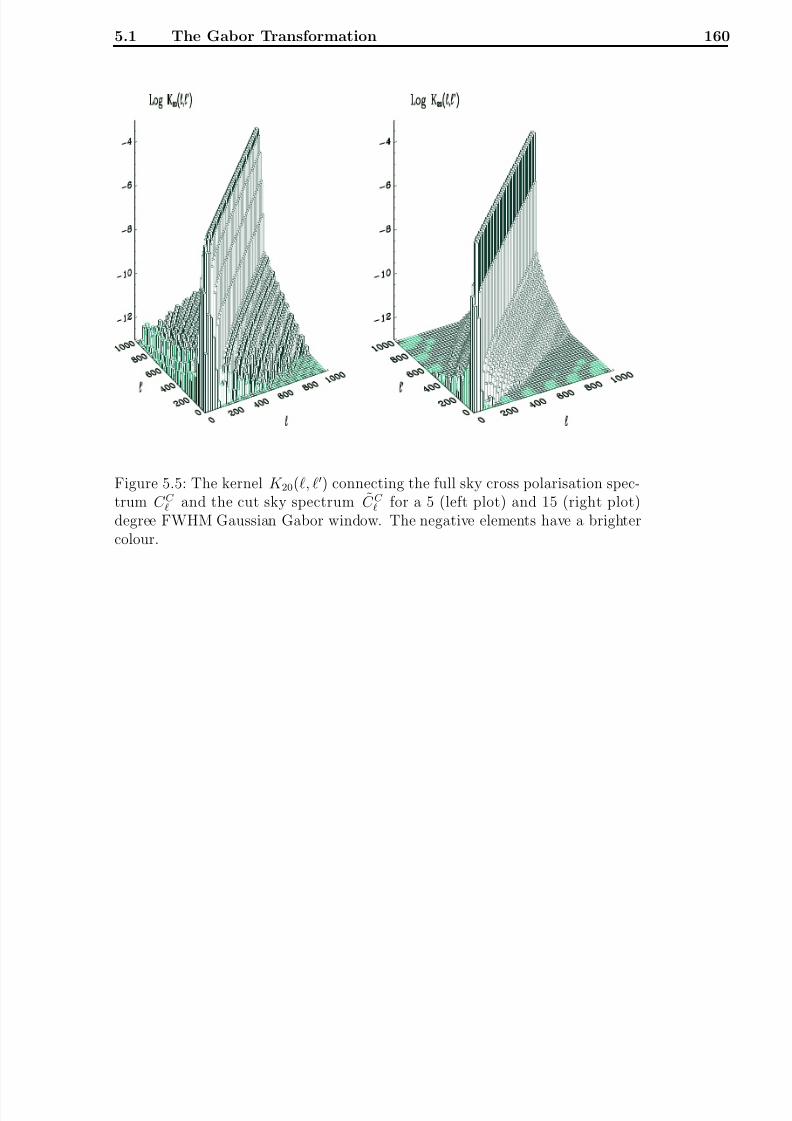
8/3/2019 Frode Kristian Hansen- Data Analysis of the Cosmic Microwave Background
http://slidepdf.com/reader/full/frode-kristian-hansen-data-analysis-of-the-cosmic-microwave-background 168/216
5.1 The Gabor Transformation 160
Figure 5.5: The kernel K 20(, ) connecting the full sky cross polarisation spec-trum C C
and the cut sky spectrum C C for a 5 (left plot) and 15 (right plot)
degree FWHM Gaussian Gabor window. The negative elements have a brightercolour.

8/3/2019 Frode Kristian Hansen- Data Analysis of the Cosmic Microwave Background
http://slidepdf.com/reader/full/frode-kristian-hansen-data-analysis-of-the-cosmic-microwave-background 169/216
5.1 The Gabor Transformation 161
Figure 5.6: Same as figure (5.5) for the corresponding tophat windows.
As for the temperature kernels, all the polarisation kernels show the samebehaviour when changing type and size of the window. When going from smallerto larger windows, the diagonals get sharper. Also the tophat kernels have morelong range correlations than the Gaussian kernels (note that all the plots havethe same vertical scale and can be compared directly).
In figure (5.7) I have plotted a cut through the different kernels at = 200 forcomparison. The cuts are made through the kernels for 5 and 15 degree FWHMGaussian Gabor windows. The first thing to note is that the temperature ker-nel K (, ), the E and B kernel K 2(, ) and the temperature-polarisation crossspectrum kernel K 20(, ) only differ for the far off-diagonal elements. At thediagonal their shape and size are the same. For this reason the relation shownin figure (4.5) between the width of the kernel and the width of the size of the
window is also valid for polarisation. This is an important result to be used forthe likelihood estimation of the polarisation power spectra in the next section. Itshows that the number of polarisation pseudo spectrum coefficients to be used inthe likelihood analysis should be the same as for the likelihood estimation of thetemperature power spectrum.
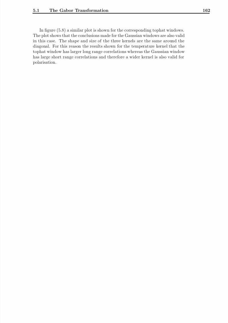
8/3/2019 Frode Kristian Hansen- Data Analysis of the Cosmic Microwave Background
http://slidepdf.com/reader/full/frode-kristian-hansen-data-analysis-of-the-cosmic-microwave-background 170/216
5.1 The Gabor Transformation 162
In figure (5.8) a similar plot is shown for the corresponding tophat windows.The plot shows that the conclusions made for the Gaussian windows are also validin this case. The shape and size of the three kernels are the same around thediagonal. For this reason the results shown for the temperature kernel that thetophat window has larger long range correlations whereas the Gaussian window
has large short range correlations and therefore a wider kernel is also valid forpolarisation.

8/3/2019 Frode Kristian Hansen- Data Analysis of the Cosmic Microwave Background
http://slidepdf.com/reader/full/frode-kristian-hansen-data-analysis-of-the-cosmic-microwave-background 171/216
5.1 The Gabor Transformation 163
Figure 5.7: A cut at = 200 through the kernels combining the full sky and cutsky power spectra. The thick solid line is the kernel K (, ) for the temperature
power spectrum, the thin solid line is the kernel K 2(, ) for E and B mode po-larisation and the dotted line is the kernel for the temperature-polarisation crosspower spectrum K 20(, ). All these kernels go together around the diagonal.They only differ for the far off-diagonal elements. The dashed line is the mixingkernel K −2(, ) which mixes the E and B mode polarisation power spectra onthe cut sky. This kernel is lower than the other kernels. The upper plot is fora 5 degree Gaussian Gabor window and the lower plot for a 15 degree FWHMGaussian window.

8/3/2019 Frode Kristian Hansen- Data Analysis of the Cosmic Microwave Background
http://slidepdf.com/reader/full/frode-kristian-hansen-data-analysis-of-the-cosmic-microwave-background 172/216
5.1 The Gabor Transformation 164
Figure 5.8: Same as figure (5.7) but for tophat windows covering the same areaon the sky.
The kernel K −2(, ) which mixes the E and B modes on the cut sky is plot-ted as a dashed line in figures (5.7) and (5.8). It is much smaller than the threeother kernels and the shape seems to differ as well. Note that the hight of themixing kernel relative to the other kernels is lower for the 15 degree window thanfor the 5 degree window. That the size of the mixing kernel relative to the otherkernels is dropping when the size of the window is increasing was to be expectedsince in the limit of full sky coverage the E -B mixing disappears and the mixingkernel must go to zero.
In figure (5.9) a cut at = 200 through the temperature kernel and the mixingkernel is shown for the 5 and 15 degree FWHM Gaussian Gabor window. Thekernels are normalised to one at the peak so that the shapes can be compared.For the Gaussian window, the shapes of the kernels still seem to be the same.

8/3/2019 Frode Kristian Hansen- Data Analysis of the Cosmic Microwave Background
http://slidepdf.com/reader/full/frode-kristian-hansen-data-analysis-of-the-cosmic-microwave-background 173/216
5.1 The Gabor Transformation 165
But the kernels for the corresponding tophat windows shown in figure (5.10) doesnot have a Gaussian shape and differs significantly from the other kernels.
Figure 5.9: A cut at = 200 through the kernel K (, ) connecting the full skytemperature power spectrum with the cut sky temperature power spectrum (solidline) and the kernel K −2(, ) which is mixing the E and B mode polarisationpower spectra on the cut sky. The upper plot is for a 5 degree FWHM GaussianGabor window and the lower plot for a 15 degree Gaussian window. The kernelsare here normalised to 1 at the peak at = 200 in order to compare the shapesof the kernels.

8/3/2019 Frode Kristian Hansen- Data Analysis of the Cosmic Microwave Background
http://slidepdf.com/reader/full/frode-kristian-hansen-data-analysis-of-the-cosmic-microwave-background 174/216
5.1 The Gabor Transformation 166
Figure 5.10: This figure is the same as figure (5.9) for tophat windows coveringthe same area on the sky.
Since the kernels for the polarisation power spectra have a shape similar tothat of the temperature power spectrum the effect of a Gabor window on theshape of the power spectrum should also be similar. This can be seen in fig-ure (5.11) and (5.12). The figures show the full sky polarisation power spectra(dashed line) C E
(figure (5.11)) and C C (figure (5.12)) for a standard CDM
model. In this model the B component of polarisation is zero. On top of thefull sky power spectra I have plotted the polarisation pseudo power spectra fora 5 and 15 degree Gaussian Gabor window (upper and lower plots respectively)
normalised so that it can be compared to the full sky spectrum. The pseudospectra for the corresponding tophat windows are plotted as dotted lines. Asexpected the shape of the polarisation pseudo spectra relative to the full skyspectra is similar to that for the temperature spectrum (figure (4.6)). One differ-ence is that the polarisation pseudo spectra for the Gaussian window do not have

8/3/2019 Frode Kristian Hansen- Data Analysis of the Cosmic Microwave Background
http://slidepdf.com/reader/full/frode-kristian-hansen-data-analysis-of-the-cosmic-microwave-background 175/216
5.1 The Gabor Transformation 167
the characteristic extra peak at low multipole which is seen in the temperaturepseudo spectrum. This peak in the temperature spectrum arose due to the steep1/( + 1) fall-off of the temperature spectrum at low multipole. The polarisationspectra do not have this steep fall-off and for this reason there is no extra peak.
Figure 5.11: The windowed polarisation power spectra C E for a 5 and 15 degree
FWHM Gaussian Gabor Gabor window cut at θC = 3σ (solid line) and for atophat window covering the same area on the sky (dotted line). All spectra arenormalised in such a way that they can be compared directly with the full skyspectrum which is shown on each plot as a dashed line. Only in the first plotare all three lines visible. In the three last plots, the full sky spectrum and the
Gaussian pseudo spectrum (dashed and solid line) are hardly distinguishable.

8/3/2019 Frode Kristian Hansen- Data Analysis of the Cosmic Microwave Background
http://slidepdf.com/reader/full/frode-kristian-hansen-data-analysis-of-the-cosmic-microwave-background 176/216
5.1 The Gabor Transformation 168
Figure 5.12: Same as figure (5.11) for the temperature-polarisation cross powerspectrum C C
.
Because of the mixing of E and B modes there is also a B polarisation com-ponent C B for the pseudo spectrum even when the input full sky C B were zero.This is shown in figure (5.13) where I have plotted the full sky spectrum C E
andthe pseudo spectra C B for the 5 and 15 degree FWHM Gaussian gabor windowsand corresponding tophat windows. The pseudo spectra are normalised so thatthey can be compared directly to the full sky spectrum. The dashed lines showthe pseudo spectra for the Gaussian window. The upper line is for the 5 degreewindow and the lower line for the 15 degree window. As expected the size of the
B component is dropping with increasing window size. The C B for the tophat
windows are plotted as dotted lines. The shape of the pseudo spectra C B forthe Gaussian windows are roughly following the shape of the full sky C E
. Thiscould be expected because the mixing kernel K −2(, ) for the Gaussian windowhas a Gaussian shape close to the diagonal, similar to the other kernels (see fig-

8/3/2019 Frode Kristian Hansen- Data Analysis of the Cosmic Microwave Background
http://slidepdf.com/reader/full/frode-kristian-hansen-data-analysis-of-the-cosmic-microwave-background 177/216
5.1 The Gabor Transformation 169
ure (5.9)). The pseudo spectra C B for the tophat windows however are muchsmoother due to the much broader kernel (figure (5.10)).
Figure 5.13: The full sky C E power spectrum plotted together with the spectra
C B on the windowed sky. The dashed lines show the B spectra for a 5 and 15degree FWHM Gaussian Gabor window (upper and lower line respectively). Thedotted lines are for the corresponding tophat windows. The pseudo spectra arenormalised so that they can be compared directly with the full sky spectrum. Inthe model used, there was no B polarisation spectrum for the full sky. The C Bshown arise due to the mixing of E and B modes on the cut sky only.
In the same way as for the temperature power spectrum, it seems that thepolarisation pseudo spectra resemble the full sky polarisation spectra when thepatches on the sky are large enough. This motivates the use of the polarisationpseudo power spectra as input to a likelihood estimation of the polarisation power
spectra in the same way as for the temperature power spectrum showed in theprevious chapter.

8/3/2019 Frode Kristian Hansen- Data Analysis of the Cosmic Microwave Background
http://slidepdf.com/reader/full/frode-kristian-hansen-data-analysis-of-the-cosmic-microwave-background 178/216
5.1 The Gabor Transformation 170
5.1.2 Rotational Invariance
I now want to show that the pseudo power spectra for polarisation are (as thetemperature power spectra) rotationally invariant under a common rotation of the sky and window. First, note that the rotation matrices D
mm are rotatingboth the normal spherical harmonics and the spin-s harmonics. This is easy to
show. Assume that one wants to rotate sY m(n) with the Euler angles (α,β ,γ ).Using the formula for the normal spherical harmonics one gets,
sY rotm (n) =
m
Dmm(α,β ,γ ) sY m(n) (5.82)
=
2 + 1
4π
m
Dmm(α,β ,γ )D
−sm(φ,θ, 0) (5.83)
= D−sm(φrot, θrot, 0)
2 + 1
4π(5.84)
= sY m(nrot), (5.85)
where nrot is the rotation of the angle n by (α,β ,γ ). This is clearly general forall spin-s harmonics. Therefore I use the method from chapter (4) to show thatpolarisation pseudo power spectra are rotationally invariant,
Consider a rotation of the sky and window by the angles (−γ − β − α). Thenthe as,m becomes,
arots,m =
dn[D(−γ − β − α)T (n)G(n)] sY ∗m(n). (5.86)
If one makes the inverse rotation of the integration angle n, one can write thisas;
a
rots,m = dnT (n)G(n)[
ˆD
∗
(αβγ ) sY
∗
m(n)], (5.87)which is just
arots,m =
m
D∗mm(αβγ )
T (n)G(n) sY ∗m(n). (5.88)
The last integral can be identified as the normal as,m.
arots,m =
m
D∗mm(αβγ )as,m. (5.89)
Thus,
arotE,m
= m
D∗
m
m(αβγ )a
E,marot
B,m=
m
D∗
m
m(αβγ )a
B,m. (5.90)
For C E,m (and analogously for C B,m and C C,m) one gets
C rotE, =
1
2 + 1
m
arotE,marot*
E,m (5.91)

8/3/2019 Frode Kristian Hansen- Data Analysis of the Cosmic Microwave Background
http://slidepdf.com/reader/full/frode-kristian-hansen-data-analysis-of-the-cosmic-microwave-background 179/216
5.2 Likelihood Analysis 171
=1
2 + 1
m
m
m
Dmm(αβγ )D∗
mm(αβγ )aE,ma∗E,m (5.92)
=1
2 + 1
mm
aE,ma∗E,m
m
Dmm(αβγ )D∗
mm(αβγ )
δmm
(5.93)
=˜
C E,. (5.94)
Since the polarisation power spectra are rotationally invariant, I will in the restof the chapter put the centre of the window on the north pole. This makes thecalculations easier while keeping the generality of the results. Now, to do thelikelihood analysis one needs to find theoretical expressions for the correlationsbetween different C Z
(Z=T,E,C).
5.2 Likelihood Analysis
For the temperature power spectrum a Gaussian likelihood ansatz was used (chap-ter (4)). Because of the similarities between the kernels of the polarisation powerspectra and the temperature power spectrum this is also to be expected for thepolarisation spectra. I will now show the results of some Monte Carlo simulationsconfirming this assumption. In this chapter I will assume that the B componentof polarisation is so small that it can be neglected. I will only concentrate on theT , E and C components of polarisation.
5.2.1 The Form of the Likelihood Function for Polarisa-
tionIn figure (5.14) and (5.15) I have plotted the probability distribution of the C E
and C C from 10000 simulations. The probability distribution (histogram) is
plotted on top of a Gaussian (dashed line) with mean and FWHM taken fromthe theoretical expressions to be derived in the next section. In these simulationsI was using a 15 degree FWHM Gaussian Gabor window with θC = 3σ. In figure(5.16) and (5.17) I show the results of similar simulations with a 15 degree FWHMGaussian Gabor window. As expected the trend is that the distributions get moreand more Gaussian for higher multipoles and for bigger windows. For the 15
FWHM window, the distribution is very close to a Gaussian for the multipoles
above = 50.

8/3/2019 Frode Kristian Hansen- Data Analysis of the Cosmic Microwave Background
http://slidepdf.com/reader/full/frode-kristian-hansen-data-analysis-of-the-cosmic-microwave-background 180/216
5.2 Likelihood Analysis 172
Figure 5.14: The probability distribution of C E taken from 10000 simulations
with a 5 FWHM Gaussian Gabor window truncated at θC = 3σ. The variable
x is given as x = (C E − < C E
>)/
< (C E − < C E
>)2 >. The dashed line is
a Gaussian with the theoretical mean and standard deviation of the C E . The
plot shows the C E distribution for = 50, = 200, = 500, and = 800. The
probabilities are normalised such that the integral over x is 1.
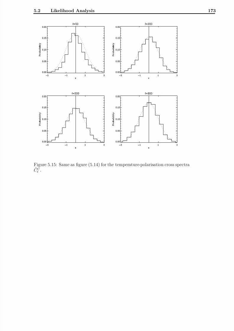
8/3/2019 Frode Kristian Hansen- Data Analysis of the Cosmic Microwave Background
http://slidepdf.com/reader/full/frode-kristian-hansen-data-analysis-of-the-cosmic-microwave-background 181/216
5.2 Likelihood Analysis 173
Figure 5.15: Same as figure (5.14) for the temperature-polarisation cross spectraC C
.

8/3/2019 Frode Kristian Hansen- Data Analysis of the Cosmic Microwave Background
http://slidepdf.com/reader/full/frode-kristian-hansen-data-analysis-of-the-cosmic-microwave-background 182/216
5.2 Likelihood Analysis 174
Figure 5.16: Same as figure (5.14) for a 15 FWHM Gaussian Gabor window.

8/3/2019 Frode Kristian Hansen- Data Analysis of the Cosmic Microwave Background
http://slidepdf.com/reader/full/frode-kristian-hansen-data-analysis-of-the-cosmic-microwave-background 183/216
5.2 Likelihood Analysis 175
Figure 5.17: Same as figure (5.15) for a 15 FWHM Gaussian Gabor window.
Figure (5.18) and (5.19) show the probability distribution for a tophat win-dow covering the same area on the sky as the Gaussian window used in figure(5.16) and (5.17). Also this distribution is very close to a Gaussian.
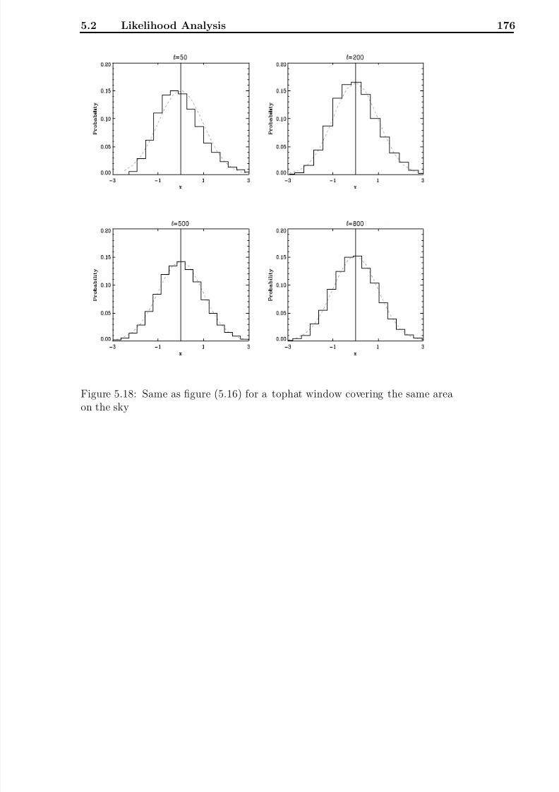
8/3/2019 Frode Kristian Hansen- Data Analysis of the Cosmic Microwave Background
http://slidepdf.com/reader/full/frode-kristian-hansen-data-analysis-of-the-cosmic-microwave-background 184/216
5.2 Likelihood Analysis 176
Figure 5.18: Same as figure (5.16) for a tophat window covering the same areaon the sky
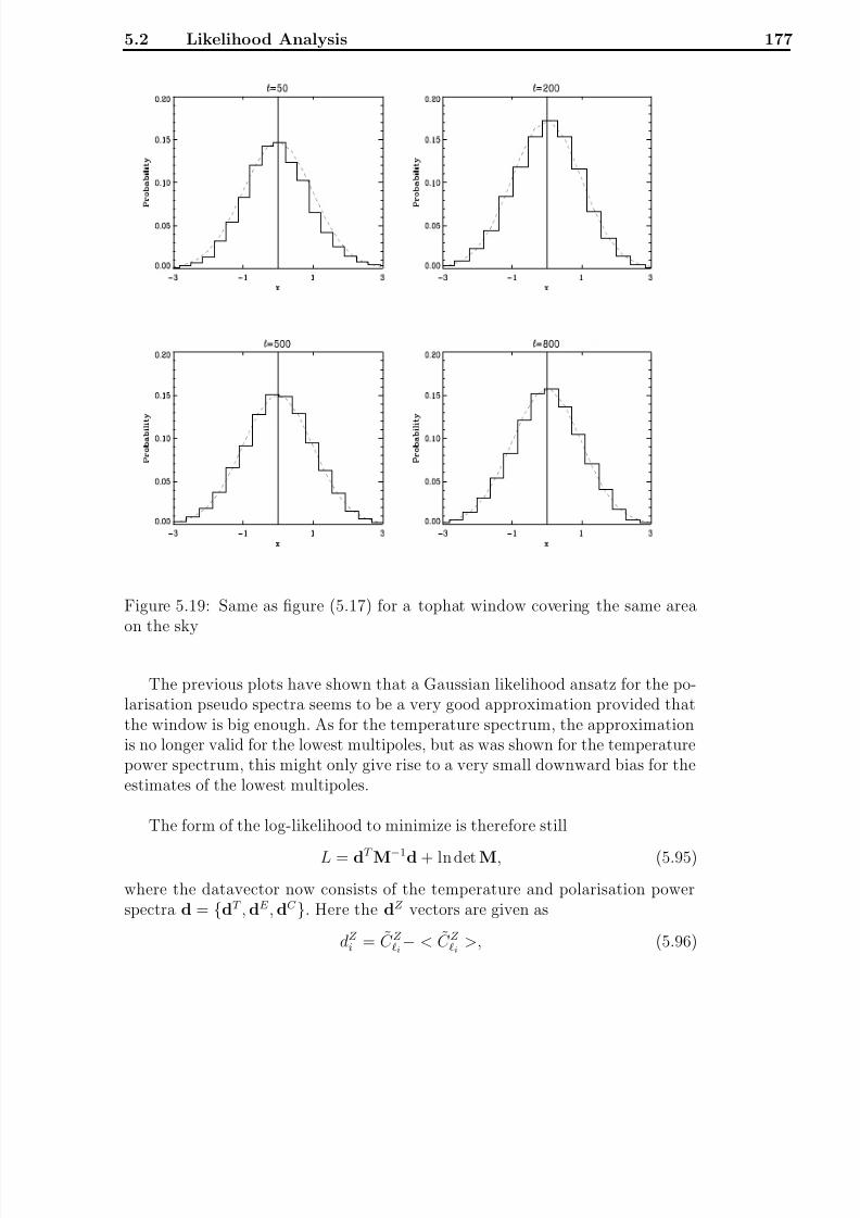
8/3/2019 Frode Kristian Hansen- Data Analysis of the Cosmic Microwave Background
http://slidepdf.com/reader/full/frode-kristian-hansen-data-analysis-of-the-cosmic-microwave-background 185/216
5.2 Likelihood Analysis 177
Figure 5.19: Same as figure (5.17) for a tophat window covering the same areaon the sky
The previous plots have shown that a Gaussian likelihood ansatz for the po-larisation pseudo spectra seems to be a very good approximation provided thatthe window is big enough. As for the temperature spectrum, the approximationis no longer valid for the lowest multipoles, but as was shown for the temperaturepower spectrum, this might only give rise to a very small downward bias for theestimates of the lowest multipoles.
The form of the log-likelihood to minimize is therefore still
L = dT M−1d + ln det M, (5.95)
where the datavector now consists of the temperature and polarisation powerspectra d = dT , dE , dC . Here the dZ vectors are given as
dZ i = C Z
i− < C Z
i>, (5.96)

8/3/2019 Frode Kristian Hansen- Data Analysis of the Cosmic Microwave Background
http://slidepdf.com/reader/full/frode-kristian-hansen-data-analysis-of-the-cosmic-microwave-background 186/216
5.2 Likelihood Analysis 178
where Z = T , E , B. Similarly the correlation matrix M will consist of blocksMZZ defined as
M ZZ ,ij =< C Z i
C Z
j> − < C Z
i>< C Z
j> . (5.97)
This structure of the datavector and correlation matrix is shown in figure (5.20).
T
E
C
<TT>
<EE>
<CC>
<TC><TE>
<EC><TE>
<TC> <EC>
Figure 5.20: The figure shows the structure of the datavector d on the left handside and the correlation matrix M on the right hand side used for joint likelihoodestimation of temperature and polarisation power spectra.
For fast likelihood estimation, it is crucial that one can calculate the aver-age pseudo spectra < C Z
> and correlation matrix M fast. The formalism inthe previous chapter which enabled fast calculations of these quantities for thetemperature power spectrum will now be extended to polarisation.
5.2.2 The Polarisation Correlation Matrix
To find the correlation matrix M for likelihood estimation of the polarisationpower spectra one needs the formulae given in equations (5.41) to (5.48). Asshown there the correlations of the pseudo am coefficients can be written in terms

8/3/2019 Frode Kristian Hansen- Data Analysis of the Cosmic Microwave Background
http://slidepdf.com/reader/full/frode-kristian-hansen-data-analysis-of-the-cosmic-microwave-background 187/216
5.2 Likelihood Analysis 179
of the h(, , m) function from chapter (4) and the H 2(, , m) and H −2(, , m)functions. These function can be quickly calculated using the important recur-sion formulae deduced in appendix (D) and (E). The starting points of theserecursions can also be quickly provided using summations and FFT as explainedin chapter (4). I will now show that the correlation function M can be expressedin terms of these functions and for this reason can be calculated quickly.
The pseudo power spectra can be written as
< C T > =
m
< aT maT ∗
m >
2 + 1, (5.98)
< C E > =
m
< aE maE ∗
m >
2 + 1, (5.99)
< C C > =
m
< aT maE ∗
m >
2 + 1. (5.100)
To find the correlation function between C for polarisation one can follow
the same steps as for the temperature correlation functions, and get,
M EE, =2
(2 + 1)(2 + 1)
m
< aE,ma∗E,m >2, (5.101)
M BB, =2
(2 + 1)(2 + 1)
m
< aB,ma∗B,m >2, (5.102)
M CC, =1
(2 + 1)(2 + 1)
m
< aE,ma∗E,m >< ama∗m > (5.103)
+ < aE,ma∗m >< aE,ma∗m >
, (5.104)
M ET, =
2
(2 + 1)(2 + 1) m < aE,ma∗
m >2
, (5.105)
M BT, =2
(2 + 1)(2 + 1)
m
| < aB,ma∗m > |2, (5.106)
M CT, =2
(2 + 1)(2 + 1)
m
< aE,ma∗m >< ama∗m >, (5.107)
M EB, =2
(2 + 1)(2 + 1)
m
| < aE,ma∗B,m > |2, (5.108)
M EC, =2
(2 + 1)(2 + 1)
m
< aE,ma∗E,m >< aE,ma∗m >, (5.109)
M BC, = 2(2 + 1)(2 + 1)
m< aE,ma∗B,m >< a∗maB,m >, (5.110)
(5.111)
where the correlation between am are given in equations (5.41) to (5.48) as sumsof h(, , m) and H ±2(, , m).

8/3/2019 Frode Kristian Hansen- Data Analysis of the Cosmic Microwave Background
http://slidepdf.com/reader/full/frode-kristian-hansen-data-analysis-of-the-cosmic-microwave-background 188/216
5.2 Likelihood Analysis 180
In figure (5.21) I have plotted the correlation matrix M T T next to the matrix
M EE . A standard CDM power spectrum without B mode polarisation was used.
The two matrices are very similar. One big difference is that the matrix for E mode polarisation is missing the ’wall’ at low multipoles present in the tempera-ture matrix. As discussed before this is because of the different shapes for the T and E power spectra at low multipoles. The temperature power spectrum drops
steeply at low while this is not the case for the E mode polarisation spectrum.
Figure 5.21: The correlation matrices M (, ) in the figure show the correlationsbetween the temperature pseudo power spectrum coefficients and between the E mode polarisation pseudo spectrum coefficients for a 15 degree FWHM GaussianGabor window. The left plot shows (< C T
C T > − < C T
>< C T >)/(< C T
><C T
>) and the right plot shows (< C E C E
> − < C E >< C E
>)/(< C E ><
C E >). A standard CDM power spectrum was used to produce the plots.
In figures (5.22) and (5.23) the M CC , M T C
, M T E and M EC
matrices areshown. All matrices are diagonally dominant and the values on the diagonals arenot differing significantly between the matrices. For this reason all the matriceshave to be computed and used in likelihood analysis.

8/3/2019 Frode Kristian Hansen- Data Analysis of the Cosmic Microwave Background
http://slidepdf.com/reader/full/frode-kristian-hansen-data-analysis-of-the-cosmic-microwave-background 189/216
5.2 Likelihood Analysis 181
Figure 5.22: The correlation matrices M (, ) in the figure show the correlationsbetween the cross-correlation pseudo power spectrum C coefficients and betweenthe temperature and cross correlation pseudo spectrum coefficients C for a 15degree FWHM Gaussian Gabor window. The left plot shows (< C C
C C > − <
C C >< C C
>)/(< C C >< C C
>) and the right plot shows (< C T C C
> − <C T
>< C C >)/(< C T
>< C C >). A standard CDM power spectrum was used
to produce the plots.

8/3/2019 Frode Kristian Hansen- Data Analysis of the Cosmic Microwave Background
http://slidepdf.com/reader/full/frode-kristian-hansen-data-analysis-of-the-cosmic-microwave-background 190/216
5.2 Likelihood Analysis 182
Figure 5.23: The correlation matrices M (, ) in the figure show the correlationsbetween the temperature and E mode polarisation pseudo spectrum coefficientsand between the E mode polarisation and cross correlation pseudo spectrumcoefficients C for a 15 degree FWHM Gaussian Gabor window. The left plotshows (< C T
C E > − < C T
>< C E >)/(< C T
>< C E >) and the right plot
shows (< C E C C
>
−< C E
>< C C >)/(< C E
>< C C >). A standard CDM
power spectrum was used to produce the plots.
5.2.3 Polarisation with Noise
Analogously to chapter (4) I will now discuss the noise pseudo power spectra andthe noise correlation matrix for polarisation. Each pixel in the temperature maphas a noise temperature n j and for the polarisation maps I assume nQ
j and nU j to
have the following properties,
< n j >= 0, < n j n j
>= δ jj
(σ
T
j )
2
, (5.112)< nQ
j >= 0, < nQ j nQ
j >= δ jj (σP j )2, (5.113)
< nU i >= 0, < nU
i nU j >= δij (σP
j )2, (5.114)

8/3/2019 Frode Kristian Hansen- Data Analysis of the Cosmic Microwave Background
http://slidepdf.com/reader/full/frode-kristian-hansen-data-analysis-of-the-cosmic-microwave-background 191/216
5.2 Likelihood Analysis 183
I also assume that there is no correlation between noise in the different maps T,Qand U. For the full sky one has,
< aN maN ∗
m > =
j
(σT j )2|Y jm|2 (5.115)
< aN 2,maN ∗
2,m > = 2 j(σP
j )2| 2Y jm|2, (5.116)
< aN −2,maN ∗
−2,m > = 2
j
(σP j )2| −2Y jm|2, (5.117)
< aN 2,maN ∗
−2,m > = 0, (5.118)
< aN E,maN ∗
E,m > = 2
j
(σP j )2(| 2Y jm|2 + | −2Y jm|2|), (5.119)
< aN B,maN ∗
B,m > = < aN E,maN ∗
E,m >, (5.120)
< aN E,maN ∗
B,m > = 0, (5.121)
which for this type of noise gives C EN = C BN
.
The pseudo a2,m coefficients can now be found using equations (5.1) and (5.2)I define
aN ±2,m =
j
(nQ j ± inU
j )G j ±2Y jm, (5.122)
for an axissymmetric Gabor window G having the value G j in pixel j. The E and B components are then similarly
aN E,m = −1
2
j
nQ
j
2Y jm + −2Y jm
+ inU
j
2Y jm − −2Y jm
G j,(5.123)
aN B,m =
1
2i j nQ
j 2Y jm − −2Y jm + inU j 2Y jm + −2Y jmG j . (5.124)
(5.125)
The correlations between these coefficients are
< aN E,maN ∗
E,m > =1
4
j
(σP
j )2
2Y jm + −2Y jm
(5.126)
×
2Y jm + −2Y jm
(5.127)
+(σP j )2
2Y jm − −2Y jm
(5.128)
× 2Y jm
−−2Y jmG2
j (5.129)
=1
2[h
2(, , m , m) (5.130)
+(−1)m+m
h2(, , −m, −m)]
≡ H 2(, , m , m), (5.131)

8/3/2019 Frode Kristian Hansen- Data Analysis of the Cosmic Microwave Background
http://slidepdf.com/reader/full/frode-kristian-hansen-data-analysis-of-the-cosmic-microwave-background 192/216
5.2 Likelihood Analysis 184
where the last line defines H 2(, , m , m). The h2(, , m , m) is defined similar
to the h(, , m , m) function in chapter (4)
h2(, , m , m) =
j
G2 j (σP
j )2 2Y jm 2Y jm , (5.132)
Note the following relation which was used to obtain equation (5.130) j
G2 j (σP
j )2 −2Y jm −2Y jm = (−1)m+m
h2(, , −m, −m). (5.133)
Again, one can see that when the Gabor window AND noise have azimuthalsymmetry this reduces simply to,
h2(, , m , m) = h
2(, , m). (5.134)
In a similar manner the other am relations can be found
< aN B,maN ∗
B,m > = < aN E,maN ∗
E,m > (5.135)
< aN E,maN ∗
B,m > = 12
i[h2(, , m , m) − (5.136)
(−1)m+m
h2(, , −m, −m)]
≡ iH −2(, , m , m), (5.137)
where the last line again defines H −2(, , m , m). The H ±2(, , m , m) functionswhich are needed to find the noise correlation matrices can be quickly calculatedusing the recursion in appendix (E).
Using these relations one can now find the polarisation pseudo spectra
< C EN >=< C BN
> = 12 + 1
m
< aN E,maN ∗
E,m >, (5.138)
< C CN > = 0 (5.139)
One can further use this to find the noise correlation matrices M N ZZ ,, defined
as,M N
ZZ , =< C ZN C Z N
> − < C ZN >< C Z N
>, (5.140)
where Z = T , E , B , C . I find,
M N TT, =
2
2 + 1 mm |< aN
maN ∗m >
|2, (5.141)
M N EE, =
2
2 + 1
mm
| < aN E,maN ∗
E,m > |2, (5.142)
M N BB, =
2
2 + 1
mm
| < aN B,maN ∗
B,m > |2, (5.143)
8/3/2019 Frode Kristian Hansen- Data Analysis of the Cosmic Microwave Background
http://slidepdf.com/reader/full/frode-kristian-hansen-data-analysis-of-the-cosmic-microwave-background 193/216
5.2 Likelihood Analysis 185
M N CC, =
1
2 + 1
mm
< aN E,maN ∗
E,m >< aN maN ∗
m >, (5.144)
M N EB, =
2
2 + 1
mm
| < aN E,maN ∗
B,m > |2, (5.145)
(5.146)
all others combinations are zero. I then find the total correlation matrix M ZZ ,
consisting of both signal and noise. As for temperature, this is not simply thesum of the correlation matrix for signal and noise, one also gets cross terms. Thefinal result is
M TT, = M S TT, + M N
TT, + (5.147)
4
2 + 1
mm
< aS maS ∗
m >< aN maN ∗
m >, (5.148)
M EE, = M S EE, + M N
EE, + (5.149)
4
2 + 1 mm < a
S
E,maS ∗
E,m >< aN
E,maN ∗
E,m >, (5.150)
M BB, = M S BB, + M N
BB, + (5.151)
4
2 + 1
mm
< aS B,maS ∗
B,m >< aN B,maN ∗
B,m >, (5.152)
M CC, = M S CC, + M N
CC, + (5.153)
1
2 + 1
mm
< aS
E,maS ∗E,m >< aN
maN ∗m > (5.154)
+ < aS maS ∗
m >< aN E,maN ∗
E,m >
, (5.155)
M TE, = M S TE, (5.156)
M TB, = M S TB, (5.157)
M TC, = M S TC, +
2
2 + 1
mm
< aS maS ∗
E,m >< aN maN ∗
m >, (5.158)
M EB, = M S EB, + M N
EB, + (5.159)
4
2 + 1
mm
< aS E,maS ∗
B,m >< aN E,maN ∗
B,m >, (5.160)
M EC, = M S EC, +
2
2 + 1 mm
< aS E,maS ∗
m >< aN E,maN ∗
E,m >, (5.161)
M BC, = M S BC, +
22 + 1
mm
< aS B,maS ∗
m >< aN B,maN ∗
E,m >, (5.162)
(5.163)

8/3/2019 Frode Kristian Hansen- Data Analysis of the Cosmic Microwave Background
http://slidepdf.com/reader/full/frode-kristian-hansen-data-analysis-of-the-cosmic-microwave-background 194/216
5.3 Results of Likelihood Estimations 186
5.3 Results of Likelihood Estimations
The likelihood estimation was carried out in the same way as for the temperaturepower spectrum. The power spectra were estimated in bins defined as
C T =
DT b
( + 1)
, b
≤ < b+1, (5.164)
C E =
DE b
( + 1), b ≤ < b+1. (5.165)
(5.166)
A similar binning does not work for for the temperature-polarisation cross cor-relation power spectrum. The reason for this is the Schwarz inequality C C
≤ C T
C E . During likelihood maximization one must make sure that the esti-
mated value of C C never exceeds
C T
C E . The way I solved this problem was
to estimate for C C / C T
C E under the constraint that this value never exceeds
1. So the binning is then
C C = DC
b
C T
C E (5.167)
=DC
b
DT
b DE b
( + 1), (5.168)
where as before b ≤ < b+1.
As an example I simulated a sky using N side = 512 resolution in Healpix anda 10 beam. I added non-uniform noise to the map. A reasonable assumption
about the size of the noise deviations for polarisation is to take σP j = √2σT j
(Zaldarriaga and Seljak 1997). This is what I used. The noise level was set sothat the signal to noise ration for the temperature power spectrum was alwayswell above 1 below the maximum multipole = 1024 whereas for the E modepolarisation power spectrum it was mostly below 1 (see figure (5.25)). This isclose to the values expected for the Planck 143GHz channel. For the analysis Iused a 15 degree Gaussian Gabor window. The result of one single estimation isshown in figure (5.25).
To test whether the method is bias or not, I did 60 Monte Carlo simulations.The result of the average of these simulations is shown in figure (5.24). Themethod seems to be unbiased also for the estimates of the polarisation powerspectra. Note that the expected noise variance taken from the approximate an-alytic formula for uniform noise (shaded areas on the plot) here fails to predictthe size of the error bars on the estimates. The expected variance taken from theinverse Fisher matrix (dashed lines) fits better with the error bars from Monte

8/3/2019 Frode Kristian Hansen- Data Analysis of the Cosmic Microwave Background
http://slidepdf.com/reader/full/frode-kristian-hansen-data-analysis-of-the-cosmic-microwave-background 195/216
5.4 Discussion 187
Carlo. The reason is that I as in chapter (4) used a noise profile with increasingnoise from the centre of the disc and down to the edges, opposite of the Gaussianwindow.
5.4 DiscussionAn extension of the power spectrum estimation method developed in chapter (4)has been made in order to estimate for polarisation power spectra. The methodhas been tested here under the assumption that the B mode polarisation is negli-gible. In this case the method appears to give unbiased estimates of the polarisa-tion power spectra also in the presence of non-uniform noise and a Gabor window.
The kernels connecting the full sky polarisation power spectra with the cutsky polarisation pseudo power spectra were studied and found to be very similarto the kernel for the temperature power spectrum. For this reason the effect of
a cut sky and a Gabor window on the polarisation power spectra is similar tothe effect on the temperature power spectrum. This explains that the method of estimating the power spectrum from the pseudo power spectrum also worked forpolarisation.
One issue which has not been studied here is the inclusion of the B modepolarisation. I demonstrated that the E and B mode polarisation power spectraare mixing on the cut sky making detections of the much weaker B componentdifficult. Further work needs to be done in order to include the B component inthe likelihood analysis.
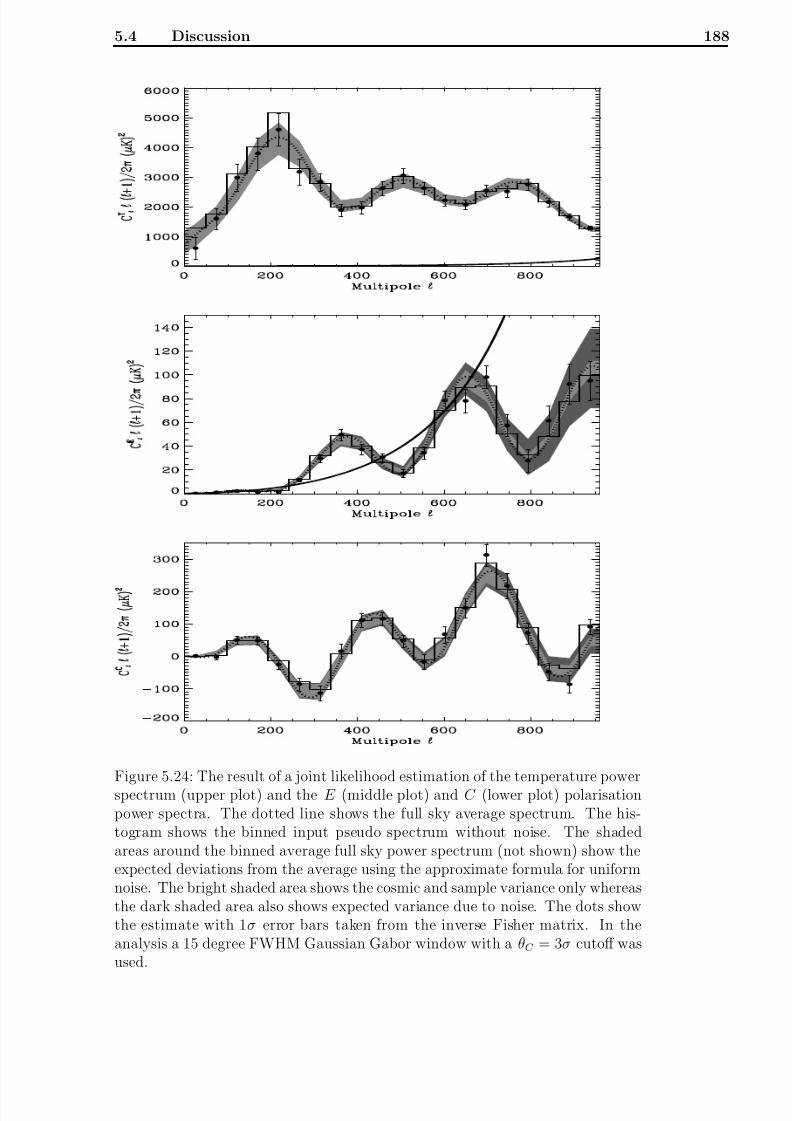
8/3/2019 Frode Kristian Hansen- Data Analysis of the Cosmic Microwave Background
http://slidepdf.com/reader/full/frode-kristian-hansen-data-analysis-of-the-cosmic-microwave-background 196/216
5.4 Discussion 188
Figure 5.24: The result of a joint likelihood estimation of the temperature powerspectrum (upper plot) and the E (middle plot) and C (lower plot) polarisationpower spectra. The dotted line shows the full sky average spectrum. The his-togram shows the binned input pseudo spectrum without noise. The shadedareas around the binned average full sky power spectrum (not shown) show theexpected deviations from the average using the approximate formula for uniformnoise. The bright shaded area shows the cosmic and sample variance only whereasthe dark shaded area also shows expected variance due to noise. The dots showthe estimate with 1σ error bars taken from the inverse Fisher matrix. In theanalysis a 15 degree FWHM Gaussian Gabor window with a θC = 3σ cutoff wasused.
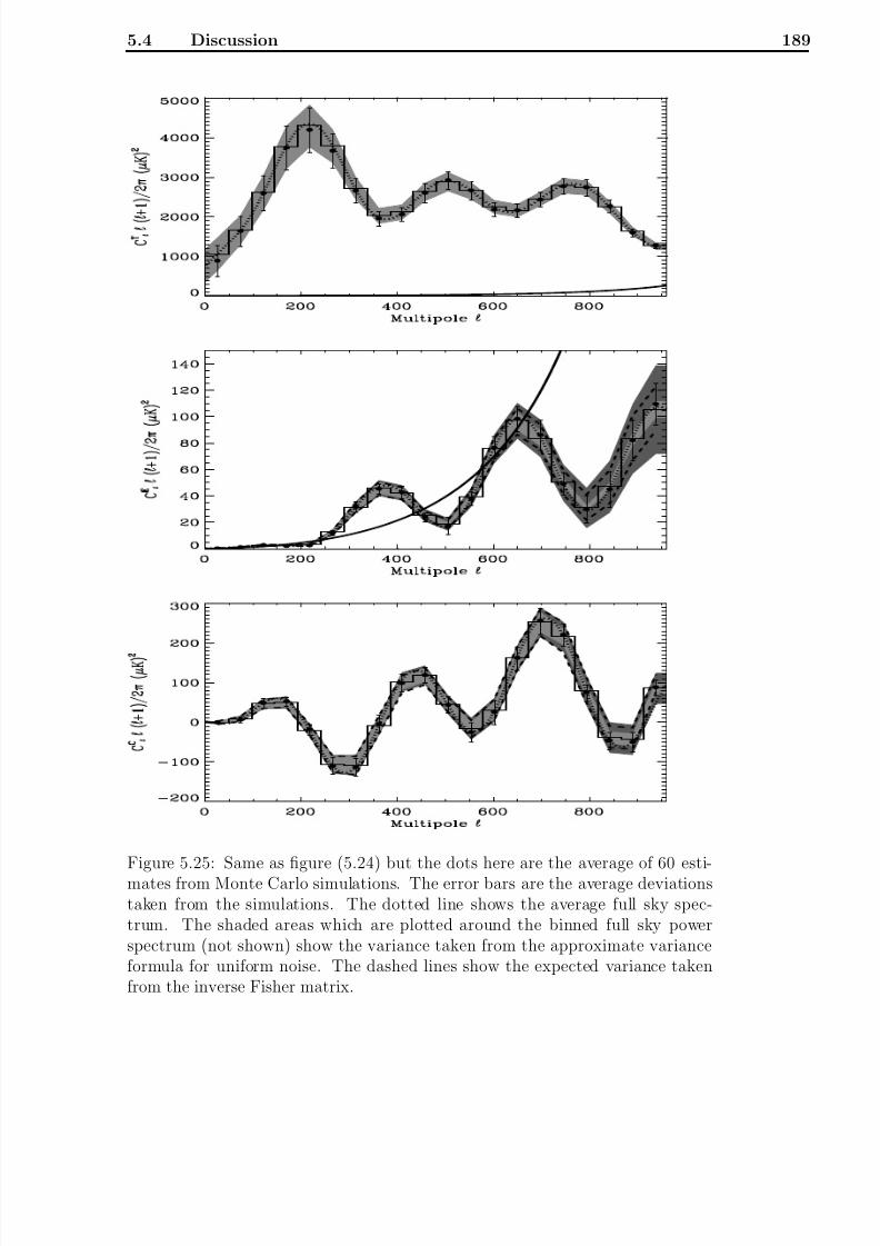
8/3/2019 Frode Kristian Hansen- Data Analysis of the Cosmic Microwave Background
http://slidepdf.com/reader/full/frode-kristian-hansen-data-analysis-of-the-cosmic-microwave-background 197/216
5.4 Discussion 189
Figure 5.25: Same as figure (5.24) but the dots here are the average of 60 esti-mates from Monte Carlo simulations. The error bars are the average deviationstaken from the simulations. The dotted line shows the average full sky spec-trum. The shaded areas which are plotted around the binned full sky powerspectrum (not shown) show the variance taken from the approximate varianceformula for uniform noise. The dashed lines show the expected variance takenfrom the inverse Fisher matrix.

8/3/2019 Frode Kristian Hansen- Data Analysis of the Cosmic Microwave Background
http://slidepdf.com/reader/full/frode-kristian-hansen-data-analysis-of-the-cosmic-microwave-background 198/216
5.4 Discussion 190

8/3/2019 Frode Kristian Hansen- Data Analysis of the Cosmic Microwave Background
http://slidepdf.com/reader/full/frode-kristian-hansen-data-analysis-of-the-cosmic-microwave-background 199/216
Appendix A
Rotation Matrices
A spherical function T (n) is rotated by the operator D(αβγ ) where αβγ are thethree Euler angles for rotations (See T.Risbo 1996) and the inverse rotation isD(−γ − β − α). For the spherical harmonic functions, this operator takes theform,
Y m(n) =
m=−
Dmm(αβγ )Y m(n), (A.1)
where Dmm has the form
Dmm(αβγ ) = eimαd
mm(β )eimγ . (A.2)
Here dmm(β ) is a real coeffecient with the following property:
dmm(β ) = d
mm(−β ). (A.3)
The D-functions also have the following property:
Dmm(αβγ ) =
m
Dmm(α2β 2γ 2)D
mm(α1β 1γ 1), (A.4)
where (αβγ ) is the result of the two consecutive rotations (α1β 1γ 1) and (α2β 2γ 2).The complex conjugate of the rotation matrices can be written as
D∗mm = (−1)m+m
D(−m)(−m). (A.5)
See also Appendix (B).

8/3/2019 Frode Kristian Hansen- Data Analysis of the Cosmic Microwave Background
http://slidepdf.com/reader/full/frode-kristian-hansen-data-analysis-of-the-cosmic-microwave-background 200/216
Appendix B
Spin-s Harmonics
The spherical harmonic functions Y m(n) can be generalized to spin-s harmonicsusing the rotation matrices in Appendix (A). The general definition is
D
−sm(φ2, θ , φ1) = 4π
2 + 1 sY m(θ, φ2)e−isφ1
, (B.1)
or in the form which will be mostly used in this thesis
sY m(θ, φ) =
2 + 1
4πD−sm(φ,θ, 0). (B.2)
The spin-s harmonics have the orthogonality and completeness relations given by dn sY m(n) sY m(n) = δδmm (B.3)
m sY m(
n) sY m(
n0) = δ(
n−
n0). (B.4)
The complex conjugate of the spin harmonics can be written
sY ∗m(n) = (−1)s+m−sY (−m)(n). (B.5)

8/3/2019 Frode Kristian Hansen- Data Analysis of the Cosmic Microwave Background
http://slidepdf.com/reader/full/frode-kristian-hansen-data-analysis-of-the-cosmic-microwave-background 201/216
Appendix C
Some Wigner Symbol Relations
Throughout the paper, the Wigner 3j Symbols will be used frequently. Here aresome relations for these symbols, which are used. The orthogonalithy relation is,
mm
m m m L
m m M = (2 + 1)−1δ
Lδ
m
M . (C.1)
The Wigner 3j Symbols can be represented as an integral of rotation matrices(see Appendix(A)),
1
8π2
d cos θdφdγD
m1m1D
m2m2D
m3m3
=
m1 m2 m3
m1 m
2 m3
.
(C.2)This expression can be reduced to,
dnY m(n)Y
m
(n)Y
m
(n) = (2 + 1)(2 + 1)(2 + 1)
4π
m m m
0 0 0 .(C.3)

8/3/2019 Frode Kristian Hansen- Data Analysis of the Cosmic Microwave Background
http://slidepdf.com/reader/full/frode-kristian-hansen-data-analysis-of-the-cosmic-microwave-background 202/216
Appendix D
Recurrence Relation
It is important for the precalculations to the likelihood analysis that the calcu-lation of h(, , m) is fast. For this reason a recurrence relation for h(, , m)would be helpfull. To speed up the calculation of the noise correlation matrix fornon axisymmetric noise, it would also help if one had a more general recurrence
relation for h(, , m , m). I will now show how to find such a recurrence forthese objects which I now call Amm
to simplify notation (and for the notation tocomply with (Wandelt, Hivon, and Gorski 2000)). The definition is again,
Amm =
b
aG(n)Y ∗m(n)Y m(n)dn, (D.1)
where G(n) = G(θ, φ) is a general function and Y m are the spherical harmonicswhich can be factorised into one part dependent on θ and one dependent on φ inthe following way,
Y m(θ, φ) = λm(cos θ)e−iφm. (D.2)
Now writing,
Amm =
d cos θλm(cos θ)λm(cos θ)
dφe−iφ(m−m)G(θ, φ) (D.3)
≡
d cos θλm(cos θ)λm(cos θ)F mm(θ), (D.4)
where F mm(θ) is simply the Fourier transform of the window at each θ. Thequantities Amm
and F mm(θ) are in general complex quantities obeying,
Amm = (Amm
)∗ F mm(θ) = (F mm(θ))∗ (D.5)
The Amm can be expressed as
Amm =
(2 + 1)(2 + 1)
2
( − m)!( − m)!
( + m)!( + m)!I m
m , (D.6)
8/3/2019 Frode Kristian Hansen- Data Analysis of the Cosmic Microwave Background
http://slidepdf.com/reader/full/frode-kristian-hansen-data-analysis-of-the-cosmic-microwave-background 203/216
195
where I mm
is defined as:
I mm
= b
aF mm(x)P m (x)P m
(x)dx. (D.7)
The following relation for the Legendre Polynomials will be used:
xP m = − m + 12 + 1
P m+1 + + m2 + 1
P m−1 (D.8)
I now define the object X mm
as
X mm
= b
aF mm(x)xP m P m
dx (D.9)
Using relation (D.8) in this definition, one gets,
X mm
= − m + 1
2 + 1I m
m(+1) +
+ m
2 + 1I m
m(−1) (D.10)
One can also exchange (, ) and (m, m) to get
X mm
= − m + 1
2 + 1I mm
(+1) + + m
2 + 1I mm
(−1) (D.11)
Taking the complex conjugate of the first expression and subtracting the last,one has
(X mm
)∗ − X mm
= 0 = − m + 1
2 + 1(I m
m(+1))
∗ + + m
2 + 1(I m
m(−1))
∗ (D.12)
− − m + 1
2 + 1
I mm
(+1)
− + m
2 + 1
I mm
(−1) (D.13)
Then setting = − 1 one gets:
I mm
=2 − 1
− m
− m + 1
2 + 1I m
m(−1)(+1) +
+ m
2 + 1I m
m(−1)(−1) − + m − 1
2 − 1I m
m(−2)
(D.14)
Using equation (D.6), one can express this as
Amm =
1
2
−m2
(42 − 1)(( + 1)2 − m2)
(2 + 1)(2 + 3)Amm(−1)(+1) (D.15)
+
(42 − 1)(2 − m2)
42 − 1Amm(−1)(−1) −
(2 + 1)(( − 1)2 − m2)
2 − 3Amm(−2)
,
which is the final recurrence relation. The Ammm elements must be provided before
the recurrence is started. Then for each (m, m), set = m +1 and let go from
8/3/2019 Frode Kristian Hansen- Data Analysis of the Cosmic Microwave Background
http://slidepdf.com/reader/full/frode-kristian-hansen-data-analysis-of-the-cosmic-microwave-background 204/216
196
and upwards, then set = m + 2 and again let go from and upwards.Continue to the desired size of . Note that, in order to get all objects up toAmm
maxmaxone need to go up to = 2max all the time during recursion. This
is because of the Amm(−1)(+1) term which all the time demands an oject indexed
( + 1) in the previous row.To start the recurrence, one can precompute the Amm
m factors fast and easily
using FFT and a sum over rings on the grid. F.ex. for the HEALPix grid, I didit the following way,
Ammm =
r
λrmmλr
m
N r−1 j=0
e−2πij/N r(m−m)Grj , (D.16)
where the last part is the Fourier transform of the Gabor window, calculated byFFT, r is ring number on the grid and j is azimuthal position on each ring. Ringr has N r pixels.
It turns out that the recurrence can be numerically unstable dependent on thewindow and multipole, and in order to avoid problems I (using double precisionnumbers) restart the recurrence with a new set of precomputed Amm
for every50th row. However for some windows and multipoles the recurrence can runfor hundreds of -rows without problems.

8/3/2019 Frode Kristian Hansen- Data Analysis of the Cosmic Microwave Background
http://slidepdf.com/reader/full/frode-kristian-hansen-data-analysis-of-the-cosmic-microwave-background 205/216
Appendix E
Extention of the Recurrence
Relation to Polarisation
For fast calculations of correlation matrices for polarisation, it would be pleasantto have a recurrence relation for
h2(, , m , m) ≡
dnG(n) 2Y m(n) 2Y m(n), (E.1)
similar to the one for h(, , m , m) in Appendix (D). Again I simplify the no-tation by calling the function Am
m . Separating the spin-2 harmonic one canwrite
2Y m(θ, φ) = 2λm(cos θ)e−imφ. (E.2)
In this way one can write Am
m as
Am
m =
dx 2λm(x) 2λm(x)
2π
0dφG(θ, φ)e−iφ(m−m)
≡F mm (x)
, (E.3)
where x = cos θ. As before I define
X m
m =
dxx 2λm(x) 2λm(x)F mm(x), (E.4)
where obviously F mm(x)∗ = F mm(x) and therefore X m
m = (X mm)∗. The next
step is to use a recurrence relation for spin-2 harmonics
x 2λm(x) = pm 2λ(+1)m(x) − qm 2λm(x) + p(−1)m 2λ(−1)m(x), (E.5)
where
pm =1
+ 1
(( + 1)2 − m2)(( + 1)2 − 4)
4( + 1)2 − 1, (E.6)
qm =2m
( + 1). (E.7)
8/3/2019 Frode Kristian Hansen- Data Analysis of the Cosmic Microwave Background
http://slidepdf.com/reader/full/frode-kristian-hansen-data-analysis-of-the-cosmic-microwave-background 206/216
198
In this way one has
X m
m = pmAm
(+1)m − qmAm
m + p(−1)mAm
(−1)m, (E.8)
X mm = pmAm
(+1)m − qmAmm + p(−1)mAm
(−1)m , (E.9)
Subtracting the complex conjugate of equation (E.9) from equation (E.8) the left
side is zero and one is left with
Am
m =1
p(−1)m
pmA
(−1)m
(+1)m + (q(−1)m − qm)A(−1)m
m (E.10)
+ p(−1)mA(−1)m
(−1)m − p(−2)mA(−2)m
m
. (E.11)
This is the recursion formula. All the Am
m can be found using the same schemeas for the scalar harmonics described in appendix (D). This equation togehterwith equation (D.15) are two of the main results in the thesis. These formulaeallow fast calculations of the couplings between scalar and tensor harmonics on
a cut sphere.

8/3/2019 Frode Kristian Hansen- Data Analysis of the Cosmic Microwave Background
http://slidepdf.com/reader/full/frode-kristian-hansen-data-analysis-of-the-cosmic-microwave-background 207/216
Bibliography
Baccigalupi, C. et al. (2000). Neural networks and the separation of cosmicmicrowave background and astrophysical signals in sky maps. MNRAS 318 ,769.
Bardeen, J. M. (1980). Gauge-invariant cosmological pertubations. Phys. Rev.D 22 , 1882.
Bartlett, J. G., M. Douspis, A. Blanchard, and M. L. Dour (2000). An ap-proximation to the likelihood function for band-power estimates of cmbanisotropies. A&ASS 146 , 507.
Bennet, C. L. et al. (1996). Four-year cobe dmr cosmic microwave backgroundobservations: Maps and basic results. ApJ 464, L1.
Bennett, C. L. et al. (1992). Preliminary separation of galactic and cosmic mi-crowave emission for the cobe differential microwave radiometer. ApJ 396 ,L7.
Bennett, C. L. et al. (1994). Cosmic temperature fluctuations from two yearsof cobe differential microwave radiometers observations. ApJ 436 , 423.
Benoit, A. et al. (2001). Archeops: A high resolution, large sky coverage balloon
experiment for mapping cmb anisotropies. astro-ph/0106152 .
Bernardis, P. D. et al. (2000). A flat universe from high-resolution maps of thecosmic microwave background radiation. Nature 404, 955.
Bersanelli, M. et al. (1996). Cobras/samba: report on the phase a study.
Bond, J. R., G. Efstathiou, and M. Tegmark (1997). Forecasting cosmic pa-rameter errors from microwave background anisotropy experiments. MN-RAS 291, L33.
Bond, J. R., A. H. Jaffe, and L. Knox (1998). Estimating the power spectrumof the cosmic microwave background. Phys.Rev.D 57 , 2117.
Bond, J. R., A. H. Jaffe, and L. Knox (2000). Radical compression of cosmicmicrowave background data. ApJ 533 , 19.
Bouchet, F. R. and R. Gispert (1999). Foregrounds and cmb experiments i.semi-analytical estimates of contamination. NewA 4, 443.

8/3/2019 Frode Kristian Hansen- Data Analysis of the Cosmic Microwave Background
http://slidepdf.com/reader/full/frode-kristian-hansen-data-analysis-of-the-cosmic-microwave-background 208/216
BIBLIOGRAPHY 200
Chandrasekhar, S. (1960). Radiative Transfer . Dover, New York.
Chiueh, T. and C. Ma (2001). The annulus-filtered e and b modes in the cmbrpolarisation. astro-ph/0101205 .
Coles, P. and F. Lucchin (1995). Cosmology . John Wiley & Sons.
Delabrouille, J. (1998). Analysis of the accuracy of a destriping method for
future cosmic microwave background mapping with the planck surveyorsatellite. A&ASS 127 , 555.
Dore, O. et al.
Dore, O., L. Knox, and A. Peel (2001). Cmb power spectrum estimation viahierarchical decomposition. astro-ph/0104443 .
Ferreira, P. G. and A. H. Jaffe (2000). Simultaneous estimation of noise andsignal in the cosmic microwave background experiments. MNRAS 312 , 89.
Gabor, D. (1946). J. Inst. Elect. Eng. 93 , 429.
Gorski et al. Homepage: http://www.eso.org/science/healpix/.
Gorski, K. M. (1994). On determining the spectrum of primordial inhomogene-ity from the cobe dmr sky maps: method. ApJ 430 , L85.
Gorski, K. M. et al. (1996). Power spectrum of primordial inhomogeneity de-termined from the four-year cobe dmr sky maps. ApJ 464, L11.
Gorski, K. M. and F. K. Hansen (2002). Cmb power spectrum estimation bycombining multiple patches on the sky. in prep..
Hanany, S. et al. (2000). Maxima-1: A measurement of the cosmic microwavebackground anisotropy on angular scales of 10 -5. ApJ 545 , L5.
Haslam, C. G. T. et al. (1981). A 408 mhz all-sky continuum survey. i - obser-vations at southern declinations and for the north polar region. A&A 100 ,209.
Hivon, E. et al. (2001). Master of the cmb anisotropy power spectrum: Afast method for statistical analysis of large and complex cmb data sets.astro-ph/0105302 .
Hobson, M. P. et al. (1999). The effect of point sources on satellite observationsof the cosmic microwave background. MNRAS 306 , 232.
Hobson, M. P., A. W. Jones, A. N. Lasenby, and F. R. Bouchet (1998).Foreground separation methods for satellite observations of the cosmic mi-
crowave background. MNRAS 300 , 1.Hobson, M. P. and J. Magueijo (1996). MNRAS 283 , 1133.
Hu, W. and N. Sugiyama (1995). Anisotropies in the cosmic microwave back-ground. ApJ 444, 489.

8/3/2019 Frode Kristian Hansen- Data Analysis of the Cosmic Microwave Background
http://slidepdf.com/reader/full/frode-kristian-hansen-data-analysis-of-the-cosmic-microwave-background 209/216
BIBLIOGRAPHY 201
Jaffe, A. H. et al. (2001). Cosmology from maxima-1, boomerang, and cobedmr cosmic microwave background observations. Phys. Rev. Lett 86 , 3475.
Jungman, G., M. Kamionkowski, A. Kosowsky, and D. N. Spergel (1996).Cosmological-paramater determination with microwave background maps.Phys. Rev. D 54, 1332.
Kamionkowski, M., A. Kosowsky, and A. Stebbins (1997). Statistics of cosmicmicrowave background polarization. Phys. Rev. D 55 , 7368.
Kogut, A. et al. (1996). High-latitude galactic emission in the cobe differentialmicrowave radiometer 2 year sky maps. ApJ 460 , 1.
Kolb, E. W. and M. S. Turner (1990). The Early Universe. Addison-WesleyPublishing Company.
Lewis, A., A. Challinor, and N. Turok (2001). Analysis of cmb polarisation onan incomplete sky. astro-ph/0106536 .
Ma, C. P. and E. Bertschinger (1995). Cosmological pertubation theory in the
synchronous and conformal newtonian gauges. ApJ 455 , 7.Maino, D. et al. (1999). The planck-lfi instrument: Analysis of the 1/f noise
and implications for the scanning strategy. A&ASS 140 , 383.
Maino, D. et al. (2001). All-sky astrophysical component separation with fastindependent component analysis (fastica). astro-ph/0108362 .
Mauskopf, P. D. et al. (2000). Measurement of a peak in the cosmic mi-crowave background power spectrum from the north american test flightof boomerang. ApJ 536 , L59.
Melchiorri, A. et al. (2000). Measurement of a peak in the cosmic mi-crowave background power spectrum from the north american test flightof boomerang. ApJ 536 , L63.
Myers, S. T., J. E. Baker, A. C. S. Readhead, and E. M. Leitch (1997). Mea-surements of the sunyaev-zeldovich effect in the nearby clusters a478, a2142,and a2256. ApJ 485 , 1.
Narlikar, J. V. and T. Padmanabhan (1991). Inflation for astronomers.ARAA 29 , 325.
Natoli, P. et al. (2001). Non-iterative methods to estimate the in-flight noiseproperties of cmb detectors. astro-ph/0110508 .
Natoli, P., G. de Gasperis, C. Gheller, and N. Vittorio (2001). A map-making
algorithm for the planck surveyor. A&A 372 , 346.
Netterfield, C. B. et al. (2000). A measurement by boomerang of multiplepeaks in the angular power spectrum of the cosmic microwave background.astro-ph/0104460 .
8/3/2019 Frode Kristian Hansen- Data Analysis of the Cosmic Microwave Background
http://slidepdf.com/reader/full/frode-kristian-hansen-data-analysis-of-the-cosmic-microwave-background 210/216
BIBLIOGRAPHY 202
Oh, S. P., D. N. Spergel, and G. Hinshaw (1999). An efficient technique to de-termine the power spectrum from cosmic microwave background sky maps.ApJ 510 , 551.
Oliveira-Costa, A. D. et al. (1997). Galactic microwave emission at degreeangular scales. ApJ 482 , 17.
Ostriker, J. P. and E. T. Vishniac (1986). Generation of microwave backgroundfluctuations from nonlinear perturbations at the era of galaxy formation.ApJ 306 , L51.
Padmanabhan, T. (1999). Aspects of gravitational clustering. astro-ph/9911374 .
Parratt, L. G. (1961). Probability and experimental errors in science. JohnWiley and Sons, Inc.
Persi, F., D. N. Spergel, R. Cen, and J. P. Ostriker (1995). Hot gas in super-clusters and microwave background distortions. ApJ 442 , 1.
Press, W. H., S. A. Teukolsky, W. T. Vetterling, and B. P. Flannery (1992).Numerical Recipes. Cambridge University Press.
Prunet, S. et al. (2001). Error estimation for the map experiment. A& A 373 ,L13.
Prunet, S., C. B. Netterfield, E. Hivon, and B. P. Crill (2000). Iterative map-making for scanning experiments. astro-ph/0006052 .
Rees, M. J. and D. W. Sciama (1968). Nature 217 , 511.
Reich, P. and W. Reich (1988). A map of spectral indices of the galactic radiocontinuum emission between 408 mhz and 1420 mhz for the entire northernsky. A&AS 74, 7.
Reynolds, R. J. (1984). A measurement of the hydrogen recombination rate inthe diffuse interstellar medium. ApJ 282 , 191.
Reynolds, R. J. (1992). The optical emission-line background and accompany-ing emissions at ultraviolet, infrared, and millimeter wavelengths. ApJ 392 ,L35.
Sachs, R. K. and A. M. Wolfe (1967). Pertubations of a cosmological mode andangular variations of the microwave background. ApJ 147 , 73.
Seljak, U. (1996). Gravitational lensing effect on cosmic microwave backgroundanisotropies: A power spectrum approach. ApJ 463 , 1.
Seljak, U. and M. Zeldariagga (1996). A line of sight approach to cosmic mi-crowave background anisotropies. ApJ 469 , 437.
Silk, J. (1968). Cosmic black-body radiation and galaxy formation. ApJ 151,459.

8/3/2019 Frode Kristian Hansen- Data Analysis of the Cosmic Microwave Background
http://slidepdf.com/reader/full/frode-kristian-hansen-data-analysis-of-the-cosmic-microwave-background 211/216
BIBLIOGRAPHY 203
Stolyarov, V., M. P. Hobson, M. A. J. Ashdown, and A. N. Lasenby (2001).All-sky component separation for the planck mission. astro-ph/0105432 .
Strohmer, T. (1997). Proc. SampTA - Sampling Theory and Applications,Aveiro/Portugal , 297.
Sunyaev, R. A. and Y. B. Zeldovich (1980). The velocity of clusters of galaxies
relative to the microwave background. the possibility of its measurement.MNRAS 190 , 413.
Szapudi, I. et al. (2001). Fast cosmic microwave background analyses via cor-relation functions. ApJ 548 , L115.
Szapudi, I., S. Prunet, and S. Colombi (2001). Fast analysis of inhomogenousmegapixel cosmic microwave background maps. ApJ 561, L11.
Taylor, A. C. (2001). The very small array. astro-ph/0109343 .
Tegmark, M. (1996). A method for extracting maximum resolution power spec-tra from microwave sky maps. MNRAS 280 , 299.
Tegmark, M. (1997a). How to make maps from the cosmic microwave back-ground data without losing information. ApJ 480 , L87.
Tegmark, M. (1997b). How to measure cmb power spectra without losing in-formation. Phys.Rev.D 55 , 5895.
Tegmark, M. et al. (1997). A high-resolution map of the cosmic microwavebackground around the north celestial pole. ApJ 474, 77.
Tegmark, M. and G. Efstathiou (1996). A method for subtracting foregroundsfrom multifrequency cmb sky maps. MNRAS 281, 1297.
Tegmark, M., A. N. Taylor, and A. F. Heavens (1997). Karhunen-loeve eigen-
value problems in cosmology: How should we tackle large data sets?ApJ 480 , 22.
Tenorio, L. (1999). Applications of wavelets to the analysis of cosmic microwavebackground maps. MNRAS 310 , 823.
Toffolatti, L. et al. (1998). Extragalactic source counts and contributions tothe anisotropies of the cosmic microwave background: predictions for theplanck surveyor mission. MNRAS 297 , 117.
Turner, M. S., M. White, and J. E. Lidsey (1993). Tensor pertubations ininflationary models as a probe of cosmology. Phys. Rev. D 48 , 4613.
Vishniac, E. T. (1987). Reionization and small-scale fluctuations in the mi-crowave background. ApJ 322 , 597.
Wandelt, B. D. (2000). Advanced methods for cosmic microwave backgrounddata analysis: the big n3 and how to beat it. astro-ph/0012416 .
8/3/2019 Frode Kristian Hansen- Data Analysis of the Cosmic Microwave Background
http://slidepdf.com/reader/full/frode-kristian-hansen-data-analysis-of-the-cosmic-microwave-background 212/216
Wandelt, B. D. and K. M. Gorski (2000). Fast convolution on the sphere.astro-ph/0008227 .
Wandelt, B. D. and F. K. Hansen (2000). Fast, exact cmb power spectrumestimation for a certain class of observational strategies. astro-ph/0106515 .
Wandelt, B. D., E. Hivon, and K. M. Gorski (2000). The pseudo-c method:
cosmic microwave background anisotropy power spectrum statistics for highprecision cosmology. astro-ph/0008111.
Watson, G. S. (2000). An exposition on inflationary cosmology. astro-ph/0005003 .
Wright, E. L. (1996). Scanning and mapping strategies for cmb experiments.proceeding of the IAS CMB Workshop astro-ph/9612006 .
Zaldariagga, M. and D. D. Harari (1995). Analytic approach to the polarizationof the cosmic microwave background in flat and open universes. Phys. Rev.D 52 , 3276.
Zaldarriaga, M. and U. Seljak (1997). An all-sky analysis of the polarisationin the microwave background. Phys. Rev. D 55 , 1830.
Zeldovich, Y. B. and R. A. Sunyaev (1969). Ap&SS 4, 301.

8/3/2019 Frode Kristian Hansen- Data Analysis of the Cosmic Microwave Background
http://slidepdf.com/reader/full/frode-kristian-hansen-data-analysis-of-the-cosmic-microwave-background 213/216
Acknowledgements
A big thanks to Kris Gorski for excellent supervision of my Ph.D. thesis, for al-ways motivating me and giving suggestions to overcome problems, and for alwaysbeing available for questions and discussions during these 3 years.
A big thanks also goes to Ben Wandelt for supervising me in a part of the thesis,for being a great teacher in CMB analysis and all other parts of physics, for givingme a lot of inspiration and for all the long nights of fruitful discussions.
Thanks to Simon White for making it possible for me to make my Ph.D. work atthe Max Planck Institute for Astrophysics.
Thanks to Anthony Banday and Eric Hivon for discussions and helpful sugges-
tions.
Cristina: Thanks a lot for your patience during the last weeks of writing myPh.D. I had far too little time for you.... And thanks for all support, energy andmotivation.
To my parents: Thanks for always supporting me and for always accepting mydecisions.
To all my friends in Munich: Thanks a lot for making Munich such a nice placeto live.
To all my collegues at MPA: Thanks for making MPA a great place to work.
And finally I want to thank the Norwegian Research Council (Norges Forskn-ingsrad) for awarding me a Ph.D. grant without which this work would have
been impossible.

8/3/2019 Frode Kristian Hansen- Data Analysis of the Cosmic Microwave Background
http://slidepdf.com/reader/full/frode-kristian-hansen-data-analysis-of-the-cosmic-microwave-background 214/216
Lebenslauf
Personliche Daten
Name: Frode Kristian HansenGeboren am: 18.04.1974 in Tønsberg, Norwegen.Staatsangehorigkeit: Norwegisch.Familienstand: ledigJetzige Adresse:Christoph-Probst-Strasse 16-727,80805 Munchen.Email:[email protected]
Hochschulausbildung
seit Okt.1999 Doktorand am Max-Planck-Institut furAstrophysik, Garching bei Munchen.
Jan.1999-Sep.1999 Doktorand am Theoretical Astro-physics Center (TAC), Kopenhagen.
Jan.1999-Dec.2001 Promotionsstipendium vom Norwegis-chen Forschungsrat. Doktorarbeit be-treut von Prof. Kris Gorski.
Jan.1997-Nov.1998 Diplomarbeit in Astrophysik betreutvon Prof. Per Lilje.
Aug.1993-Dec.1996 Mathematik-, Physik- und As-trophysikkurse mit Examen jedesSemester.
Aug.1993-Nov.1998 Astrophysikstudium an der Universitatin Oslo.
Schulausbildung
Aug.1990-Jun.1993 Tønsberg Gymnasium (Norwegen),Linie fur Naturwissenschaft.
Aug.1981-Jun.1990 Grundschule in Tønsberg (Norwegen)

8/3/2019 Frode Kristian Hansen- Data Analysis of the Cosmic Microwave Background
http://slidepdf.com/reader/full/frode-kristian-hansen-data-analysis-of-the-cosmic-microwave-background 215/216

8/3/2019 Frode Kristian Hansen- Data Analysis of the Cosmic Microwave Background
http://slidepdf.com/reader/full/frode-kristian-hansen-data-analysis-of-the-cosmic-microwave-background 216/216