Forensic Analysis of Database Tampering - Arizona Computer Science
47
30 Forensic Analysis of Database Tampering KYRIACOS E. PAVLOU and RICHARD T. SNODGRASS University of Arizona Regulations and societal expectations have recently expressed the need to mediate access to valu- able databases, even by insiders. One approach is tamper detection via cryptographic hashing. This article shows how to determine when the tampering occurred, what data was tampered with, and perhaps, ultimately, who did the tampering, via forensic analysis. We present four successively more sophisticated forensic analysis algorithms: the Monochromatic, RGBY, Tiled Bitmap, and a3D algorithms, and characterize their “forensic cost” under worst-case, best-case, and average- case assumptions on the distribution of corruption sites. A lower bound on forensic cost is derived, with RGBY and a3D being shown optimal for a large number of corruptions. We also provide vali- dated cost formulæ for these algorithms and recommendations for the circumstances in which each algorithm is indicated. Categories and Subject Descriptors: H.2.0 [Database Management]: General—Security, integrity, and protection General Terms: Algorithms, Performance, Security Additional Key Words and Phrases: a3D algorithm, compliant records, forensic analysis algorithm, forensic cost, Monochromatic algorithm, Polychromatic algorithm, RGBY algorithm, Tiled Bitmap algorithm. ACM Reference Format: Pavlou, K. E. and Snodgrass, R. T. 2008. Forensic analysis of database tampering. ACM Trans. Datab. Syst. 33, 4, Article 30 (November 2008), 47 pages. DOI = 10.1145/1412331.1412342 http://doi.acm.org/10.1145/1412331.1412342 1. INTRODUCTION Recent regulations require many corporations to ensure trustworthy long- term retention of their routine business documents. The US alone has over 10,000 regulations [Gerr et al. 2003] that mandate how business data should be managed [Chan et al. 2004; Wingate 2003], including the Health Insurance Portability and Accountability Act: HIPAA [1996], Canada’s PIPEDA NSF grants IIS-0415101, IIS-0639106, and EIA-0080123 and a grant from Microsoft provided partial support for this work. Authors’ address: K. E. Pavlou and R. T. Snodgrass, Department of Computer Science, University of Arizona, Tucson, AZ 85721-0077; email: {kpavlou, rts}@cs.arizona.edu. Permission to make digital or hard copies of part or all of this work for personal or classroom use is granted without fee provided that copies are not made or distributed for profit or direct commercial advantage and that copies show this notice on the first page or initial screen of a display along with the full citation. Copyrights for components of this work owned by others than ACM must be honored. Abstracting with credit is permitted. To copy otherwise, to republish, to post on servers, to redistribute to lists, or to use any component of this work in other works requires prior specific permission and/or a fee. Permissions may be requested from Publications Dept., ACM, Inc., 2 Penn Plaza, Suite 701, New York, NY 10121-0701 USA, fax +1 (212) 869-0481, or [email protected]. C 2008 ACM 0362-5915/2008/11-ART30 $5.00 DOI 10.1145/1412331.1412342 http://doi.acm.org/ 10.1145/1412331.1412342 ACM Transactions on Database Systems, Vol. 33, No. 4, Article 30, Publication date: November 2008.
Transcript of Forensic Analysis of Database Tampering - Arizona Computer Science

30
Forensic Analysis of Database Tampering
KYRIACOS E. PAVLOU and RICHARD T. SNODGRASS
University of Arizona
Regulations and societal expectations have recently expressed the need to mediate access to valu-
able databases, even by insiders. One approach is tamper detection via cryptographic hashing. This
article shows how to determine when the tampering occurred, what data was tampered with, and
perhaps, ultimately, who did the tampering, via forensic analysis. We present four successively
more sophisticated forensic analysis algorithms: the Monochromatic, RGBY, Tiled Bitmap, and
a3D algorithms, and characterize their “forensic cost” under worst-case, best-case, and average-
case assumptions on the distribution of corruption sites. A lower bound on forensic cost is derived,
with RGBY and a3D being shown optimal for a large number of corruptions. We also provide vali-
dated cost formulæ for these algorithms and recommendations for the circumstances in which each
algorithm is indicated.
Categories and Subject Descriptors: H.2.0 [Database Management]: General—Security, integrity,and protection
General Terms: Algorithms, Performance, Security
Additional Key Words and Phrases: a3D algorithm, compliant records, forensic analysis algorithm,
forensic cost, Monochromatic algorithm, Polychromatic algorithm, RGBY algorithm, Tiled Bitmap
algorithm.
ACM Reference Format:Pavlou, K. E. and Snodgrass, R. T. 2008. Forensic analysis of database tampering. ACM Trans.
Datab. Syst. 33, 4, Article 30 (November 2008), 47 pages. DOI = 10.1145/1412331.1412342
http://doi.acm.org/10.1145/1412331.1412342
1. INTRODUCTION
Recent regulations require many corporations to ensure trustworthy long-term retention of their routine business documents. The US alone hasover 10,000 regulations [Gerr et al. 2003] that mandate how business datashould be managed [Chan et al. 2004; Wingate 2003], including the HealthInsurance Portability and Accountability Act: HIPAA [1996], Canada’s PIPEDA
NSF grants IIS-0415101, IIS-0639106, and EIA-0080123 and a grant from Microsoft provided
partial support for this work.
Authors’ address: K. E. Pavlou and R. T. Snodgrass, Department of Computer Science, University
of Arizona, Tucson, AZ 85721-0077; email: {kpavlou, rts}@cs.arizona.edu.
Permission to make digital or hard copies of part or all of this work for personal or classroom use is
granted without fee provided that copies are not made or distributed for profit or direct commercial
advantage and that copies show this notice on the first page or initial screen of a display along
with the full citation. Copyrights for components of this work owned by others than ACM must be
honored. Abstracting with credit is permitted. To copy otherwise, to republish, to post on servers,
to redistribute to lists, or to use any component of this work in other works requires prior specific
permission and/or a fee. Permissions may be requested from Publications Dept., ACM, Inc., 2 Penn
Plaza, Suite 701, New York, NY 10121-0701 USA, fax +1 (212) 869-0481, or [email protected]© 2008 ACM 0362-5915/2008/11-ART30 $5.00 DOI 10.1145/1412331.1412342 http://doi.acm.org/
10.1145/1412331.1412342
ACM Transactions on Database Systems, Vol. 33, No. 4, Article 30, Publication date: November 2008.

30:2 • K. E. Pavlou and R. T. Snodgrass
[2000], Sarbanes-Oxley Act [2002], and PITAC’s advisory report on healthcare [Agrawal et al. 2007]. Due to these and to widespread news coverage ofcollusion between auditors and the companies they audit (e.g., Enron, World-Com), which helped accelerate passage of the aforementioned laws, there hasbeen interest within the file systems and database communities about built-inmechanisms to detect or even prevent tampering.
One area in which such mechanisms have been applied is audit log security.The Orange Book [Department of Defense 1985] informally defines audit logsecurity in Requirement 4: “Audit information must be selectively kept and pro-tected so that actions affecting security can be traced to the responsible party.A trusted system must be able to record the occurrences of security-relevantevents in an audit log . . . Audit data must be protected from modification andunauthorized destruction to permit detection and after-the-fact investigationsof security violations.”
The need for audit log security goes far beyond just the financial and med-ical information systems mentioned previously. The 1997 U.S. Food and DrugAdministration (FDA) regulation “part 11 of Title 21 of the Code of Fed-eral Regulations; Electronic Records; Electronic Signatures” (known affection-ately as “21 CFR Part 11” or even more endearingly as “62 FR 13430”) re-quires that analytical laboratories collecting data used for new drug approvalemploy “user independent computer-generated time stamped audit trails”[FDA 2003].
Audit log security is one component of more general record managementsystems that track documents and their versions, and ensure that a previousversion of a document cannot be altered. As an example, digital notarizationservices such as Surety (www.surety.com), when provided with a digital docu-ment, generate a notary ID through secure one-way hashing, thereby lockingthe contents and time of the notarized documents [Haber and Stornetta 1991].Later, when presented with a document and the notary ID, the notarizationservice can ascertain whether that specific document was notarized, and if so,when.
Compliant records are those required by myriad laws and regulations to fol-low certain “processes by which they are created, stored, accessed, maintained,and retained” [Gerr et al. 2003]. It is common to use Write-Once-Read-Many(WORM) storage devices to preserve such records [Zhu and Hsu 2005]. Theoriginal record is stored on a write-once optical disk. As the record is modified,all subsequent versions are also captured and stored, with metadata recordingthe timestamp, optical disk, filename, and other information on the record andits versions.
Such approaches cannot be applied directly to high-performance databases.A copy of the database cannot be versioned and notarized after each transaction.Instead, audit log capabilities must be moved into the DBMS. We previouslyproposed an innovative approach in which cryptographically-strong one-wayhash functions prevent an intruder, including an auditor or an employee oreven an unknown bug within the DBMS itself, from silently corrupting the auditlog [Snodgrass et al. 2004]. This is accomplished by hashing data manipulated
ACM Transactions on Database Systems, Vol. 33, No. 4, Article 30, Publication date: November 2008.
Forensic Analysis of Database Tampering • 30:3
by transactions and periodically validating the audit log database to detectwhen it has been altered.
The question then arises, what do you do when an intrusion has been de-tected? At that point, all you know is that at some time in the past, data some-where in the database has been altered. Forensic analysis is needed to ascertainwhen the intrusion occurred, what data was altered, and ultimately, who theintruder is.
In this article, we provide a means of systematically performing forensicanalysis after an intrusion of an audit log has been detected. (The identificationof the intruder is not explicitly dealt with.) We first summarize the originallyproposed approach, which provides exactly one bit of information: has the au-dit log been tampered with? We introduce a schematic representation termeda corruption diagram for analyzing an intrusion. We then consider how addi-tional validation steps provide a sequence of bits that can dramatically narrowdown the when and where. We examine the corruption diagram for this initialapproach; this diagram is central in all of our further analyses. We characterizethe forensic cost of this algorithm, defined as a sum of the external notarizationsand validations required and the area of the uncertainty region(s) in the cor-ruption diagram. We look at the more complex case in which the timestamp ofthe data item is corrupted, along with the data. Such an action by the intruderturns out to greatly increase the uncertainty region. Along the way, we identifysome configurations that turn out not to improve the precision of the forensicalgorithms, thus helping to cull the most appropriate alternatives.
We then consider computing and notarizing additional sequences of hashvalues. We first consider the Monochromatic Algorithm; we then present theRGBY, Tiled Bitmap, and a3D Algorithms. For each successively more powerfulalgorithm, we provide an informal presentation using the corruption diagram,the algorithm in pseudocode, and then a formal analysis of the algorithm’sasymptotic run time and forensic cost. We end with a discussion of relatedand future work. The appendix includes an analysis of the forensic cost for thealgorithms, using worst-case, best-case, and average-case assumptions on thedistribution of corruption sites.
2. TAMPER DETECTION VIA CRYPTOGRAPHIC HASH FUNCTIONS
In this section, we summarize the tamper detection approach we previouslyproposed and implemented [Snodgrass et al. 2004]. We just give the gist of ourapproach, so that our forensic analysis techniques can be understood.
This basic approach differentiates two execution phases: online processing,in which transactions are run and hash values are digitally notarized, andvalidation, in which the hash values are recomputed and compared with thosepreviously notarized. It is during validation that tampering is detected, whenthe just-computed hash value doesn’t match those previously notarized. The twoexecution phases constitute together the normal processing phase as opposedto the forensic analysis phase. Figure 1 illustrates the two phases of normalprocessing.
ACM Transactions on Database Systems, Vol. 33, No. 4, Article 30, Publication date: November 2008.

30:4 • K. E. Pavlou and R. T. Snodgrass
Fig. 1. Online processing (a) and Audit log validation (b).
In Figure 1(a), the user application performs transactions on the database,which insert, delete, and update the rows of the current state. Behind thescenes, the DBMS maintains the audit log by rendering a specified relation as atransaction-time table. This instructs the DBMS to retain previous tuples dur-ing update and deletion, along with their insertion and deletion/update time(the start and stop timestamps), in a manner completely transparent to theuser application [Bair et al. 1997]. An important property of all data storedin the database is that it is append-only: modifications only add information;no information is ever deleted. Hence if old information is changed in any way,then tampering has occurred. Oracle 11g supports transaction-time tables withits workspace manager [Oracle Corporation 2007]. The Immortal DB projectaims to provide transaction time database support built into Microsoft SQLServer [Lomet et al. 2005]. How this information is stored (in the log, in the re-lational store proper, in a separate “archival store” [Ahn and Snodgrass 1988])is not that critical in terms of forensic analysis, as long as previous tuples areaccessible in some way. In any case, the DBMS retains for each tuple hiddenStart and Stop times, recording when each change occurred. The DBMS en-sures that only the current state of the table is accessible to the application,with the rest of the table serving as the audit log. Alternatively, the table itselfcould be viewed by the application as the audit log. In that case, the applicationonly makes insertions to the audited table; these insertions are associated witha monotonically increasing Start time.
We use a digital notarization service that, when provided with a digital docu-ment, provides a notary ID. Later, during audit log validation, the notarizationservice can ascertain, when presented with the supposedly unaltered documentand the notary ID, whether that document was notarized, and if so, when.
On each modification of a tuple, the DBMS obtains a timestamp, computesa cryptographically strong one-way hash function of the (new) data in the tupleand the timestamp, and sends that hash value, as a digital document, to thenotarization service, obtaining a notary ID. The DBMS stores that ID in thetuple.
Later, an intruder gets access to the database. If he changes the data ora timestamp, the ID will now be inconsistent with the rest of the tuple. The
ACM Transactions on Database Systems, Vol. 33, No. 4, Article 30, Publication date: November 2008.

Forensic Analysis of Database Tampering • 30:5
intruder cannot manipulate the data or timestamp so that the ID remainsvalid, because the hash function is one-way. Note that this holds even when theintruder has access to the hash function itself. He can instead compute a newhash value for the altered tuple, but that hash value won’t match the one thatwas notarized.
An independent audit log validation service later scans the database (as il-lustrated in Figure 1(b)), hashes the data and the timestamp of each tuple, andprovides it with the ID to the notarization service, which then checks the no-tarization time with the stored timestamp. The validation service then reportswhether the database and the audit log are consistent. If not, either or bothhave been compromised.
Few assumptions are made about the threat model. The system is secureuntil an intruder gets access, at which point he has access to everything: theDBMS, the operating system, the hardware, and the data in the database.We still assume that the notarization and validation services remain in thetrusted computing base. This can be done by making them geographically andperhaps organizationally separate from the DBMS and the database, therebyeffecting correct tamper detection even when the tampering is done by highlymotivated insiders. (A recent FBI study indicates almost half of attacks wereby insiders [CSI/FBI 2005].)
The basic mechanism just described provides correct tamper detection. Ifan intruder modifies even a single byte of the data or its timestamp, the inde-pendent validator will detect a mismatch with the notarized document, therebydetecting the tampering. The intruder could simply re-execute the transactions,making whatever changes he wanted, and then replace the original databasewith his altered one. However, the notarized documents would not match intime. Avoiding tamper detection comes down to inverting the cryptographically-strong one-way hash function. Refinements to this approach and performancelimitations are addressed elsewhere [Snodgrass et al. 2004].
A series of implementation optimizations minimize notarization service in-teraction and speed up processing within the DBMS: opportunistic hashing,linked hashing, and a transaction ordering list. In concert, these optimizationsreduce the run time overhead to just a few percent of the normal running timeof a high-performance transaction processing system [Snodgrass et al. 2004].For our purposes, the only detail that is important for forensic analysis is that,at commit time, the transaction’s hash value and the previous hash value arehashed together to obtain a new hash value. Thus the hash value of each indi-vidual transaction is linked in a sequence, with the final value being essentiallya hash of all changes to the database since the database was created. For moredetails on exactly how the tamper detection approach works, please refer toour previous paper [Snodgrass et al. 2004], which presents the threat modelused by this approach, discusses performance issues, and clarifies the role ofthe external notarization service.
The validator provides a vital piece of information, that tampering has takenplace, but doesn’t offer much else. Since the hash value is the accumulationof every transaction ever applied to the database, we don’t know when thetampering occurred, or what portion of the audit log was corrupted. (Actually,
ACM Transactions on Database Systems, Vol. 33, No. 4, Article 30, Publication date: November 2008.

30:6 • K. E. Pavlou and R. T. Snodgrass
Table I. Summary of Notation Used
Symbol Name Definition
CE Corruption event An event that compromises the database
The validation of the audit logVE Validation eventby the notarization service
The notarization of a documentNE Notarization event(hash value) by the notarization service
lc Corruption locus data The corrupted data
tn Notarization time The time instant of a NEtv Validation time The time instant of a VEtc Corruption time The time instant of a CE
tl Locus time The time instant that lc was stored
IV Validation interval The time between two successive VEs
IN Notarization interval The time between two successive NEs
Temporal detection Finest granularity chosen to expressRtresolution temporal bounds uncertainty of a CE
Spatial detection Finest granularity chosen to expressRsresolution spatial bounds uncertainty of a CE
Time of most recent The time instant of the last NE whosetRVSvalidation success revalidation yielded a true result
tFVF Time of first validation failure Time instant at which the CE is first detected
Upper bound of the spatial uncertaintyUSB Upper spatial boundof the corruption region
Lower bound of the spatial uncertaintyLSB Lower spatial boundof the corruption region
Upper bound of the temporal uncertaintyUTB Upper temporal boundof the corruption region
Lower bound of the temporal uncertaintyLTB Lower temporal boundof the corruption region
V Validation factor The ratio IV /IN
N Notarization factor The ratio IN /Rs
the validator does provide a very vague sense of when: sometime before now,and where: somewhere in the data stored before now.)
It is the subject of the rest of this article to examine how to perform a forensicanalysis of a detected tampering of the database.
3. DEFINITIONS
We now examine tamper detection in more detail. Suppose that we have justdetected a corruption event (CE), which is any event that corrupts the dataand compromises the database. (Table I summarizes the notation used in thisarticle. Some of the symbols are introduced in subsequent sections.)
The corruption event could be due to an intrusion, some kind of human inter-vention, a bug in the software (be it the DBMS or the file system or somewherein the operating system), or a hardware failure, either in the processor or onthe disk. There exists a one-to-one correspondence between a CE and its cor-ruption time (tc), which is the actual time instant (in seconds) at which a CEhas occurred.
The CE was detected during a validation of the audit log by the notarizationservice, termed a validation event (VE). A validation can be scheduled (that is,
ACM Transactions on Database Systems, Vol. 33, No. 4, Article 30, Publication date: November 2008.

Forensic Analysis of Database Tampering • 30:7
is periodic) or could be an ad hoc VE. The time (instant) at which a VE occurredis termed the time of validation event, and is denoted by tv. If validations areperiodic, the time interval between two successive validation events is termedthe validation interval, or IV . Tampering is indicated by a validation failure,in which the validation service returns false for the particular query of a hashvalue and a notarization time. What is desired is a validation success, in whichthe notarization service returns true, stating that everything is OK: the datahas not been tampered with.
The validator compares the hash value it computes over the data with thehash value that was previously notarized. A notarization event (NE) is the no-tarization of a document (specifically, a hash value) by the notarization service.As with validation, notarization can be scheduled (is periodic) or can be anad hoc notarization event. Each NE has an associated notarization time (tn),which is a time instant. If notarizations are periodic, the time interval be-tween two successive notarization events is termed the notarization interval,or IN .
There are several variables associated with each corruption event. Thefirst is the data that has been corrupted, which we term the corruption locusdata (lc).
Forensic analysis involves temporal detection, the determination of the cor-ruption time, tc. Forensic analysis also involves spatial detection, the determi-nation of where, that is, the location in the database of the data altered in a CE.(Note that the use of the adjective “spatial” does not refer to a spatial database,but rather where in the database the corruption occurred.)
Recall that each transaction is hashed. Therefore, in the absence of otherinformation, such as a previous dump (copy) of the database, the best a forensicanalysis can do is to identify the particular transaction that stored the datathat was corrupted. Instead of trying to ascertain the corruption locus data,we will instead be concerned with the locus time (tl ), the time instant thatlocus data (lc) was originally stored. The locus time specifically refers to thetime instant when the transaction storing the locus data commits. (Note thathere we are referring to the specific version of the data that was corrupted.This version might be the original version inserted by the transaction, or asubsequent version created through an update operation.) Hence the task offorensic analysis is to determine two times, tc and tl .
A CE can have many lcs (and hence, many tl s) associated with it, termedmulti-locus: an intruder (hardware failure, etc.) might alter many tuples. A CEhaving only one lc (such as due to an intruder hoping to remain undetected bymaking a single, very particular change) is termed a single-locus CE.
The finest spatial granularity of the corrupted data would be an explicitattribute of a tuple, or a particular timestamp attribute. However, this provesto be costly and hence we define Rs, which is the finest granularity chosen toexpress the uncertainty of the spatial bounds of a CE. Rs is called the spatialdetection resolution. This is chosen by the DBA.
Similarly, the finest granularity chosen by the DBA to express the uncer-tainty of the temporal bounds of a CE is the temporal detection resolution,or Rt .
ACM Transactions on Database Systems, Vol. 33, No. 4, Article 30, Publication date: November 2008.
30:8 • K. E. Pavlou and R. T. Snodgrass
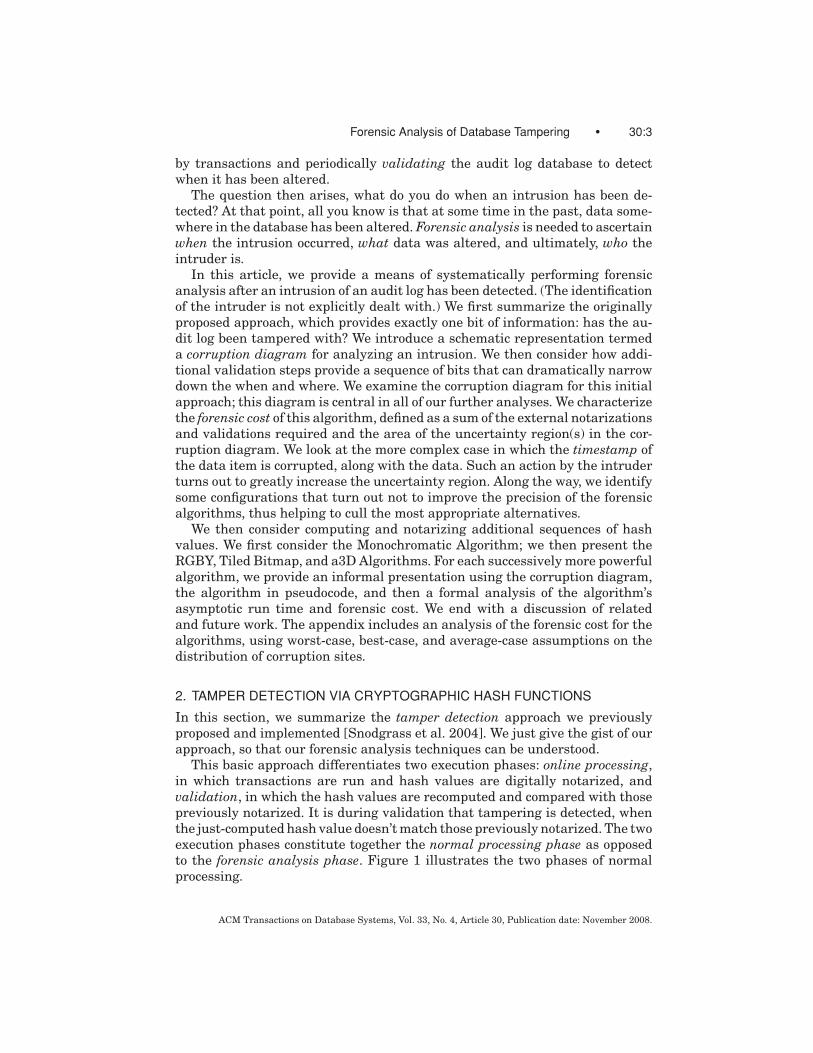
Fig. 2. Corruption diagram for a data-only single-locus retroactive corruption event.
4. THE CORRUPTION DIAGRAM
To explain forensic analysis, we introduce the Corruption Diagram, which is agraphical representation of CE(s) in terms of the temporal-spatial dimensionsof a database. We have found these diagrams to be very helpful in understand-ing and communicating the many forensic algorithms we have considered, andso we will use them extensively in this article.
Definition. A corruption diagram is a plot in R2 having its ordinate associ-
ated with real time and its abscissa associated with a partition of the databaseaccording to transaction time. This diagram depicts corruption events and isannotated with hash chains and relevant notarization and validation events.At the end of forensic analysis, this diagram can be used to visualize theregions (⊂ R
2) where corruption has occurred.
Let us first consider the simplest case. During validation, we have detecteda corruption event. Though we don’t know it (yet), assume that this corruptionevent is a single-locus CE. Furthermore, assume that the CE just altered thedata of a tuple; no timestamps were changed.
Figure 2 illustrates our simple corruption event. While this figure may ap-pear to be complex, the reader will find that it succinctly captures all theimportant information regarding what is stored in the database, what is
ACM Transactions on Database Systems, Vol. 33, No. 4, Article 30, Publication date: November 2008.

Forensic Analysis of Database Tampering • 30:9
notarized, and what can be determined by the forensic analysis algorithm aboutthe corruption event.
The x-axis represents when the data are stored in the database. The databasewas created at time 0, and is modified by transactions whose commit timeis monotonically increasing along the x-axis. (In temporal database terminol-ogy [Jensen and Dyreson 1998], the x-axis represents the transaction time ofthe data.) In this diagram, time moves inexorably to the right.
This axis is labeled “Where.” The database grows monotonically as tuplesare appended (recall that the database is append-only). As above, we designatewhere a tuple or attribute is in the database by the time of the transactionthat inserted that tuple or attribute. The unit of the x-axis is thus (transaction-commit) time. We delimit the days by marking each midnight, or, more accu-rately, the time of the last transaction to commit before midnight.
A 45-degree line is shown and is termed the action line, since all the action inthe database occurs on this line. The line terminates at the point labeled “FVF,”which is the validation event at which we first became aware of tampering. Thetime of first validation failure (or tFVF) is the time at which the corruption is firstdetected. (Hence the name: a corruption diagram always terminates at the VEthat detected the corruption event.) Note that tFVF is an instance of a tv, in thattFVF is a specific instance of the time of a validation event, generically denotedby tv. Also note that in every corruption diagram, tFVF coincides with the currenttime. For example, in Figure 2 the VE associated with tFVF occurs on the actionline, at its terminus, and turns out to be the fourth such validation event, VE4.
The actual corruption event is shown as a point labeled “CE,” which alwaysresides above or on the action line, and below the last VE. If we project thispoint onto the x-axis, we learn where (in terms of the locus of corruption, lc)the corruption event occurred. Hence the x-axis, which being ostensibly committime, can also be viewed as a spatial dimension, labeled in locus time instants(tl ). This is why we term the x-axis the where axis.
The y-axis represents the temporal dimension (actual time-line) of thedatabase, labeled in time instants. Any point on the action line thus indicatesa transaction committing at a particular transaction time (a coordinate on thex-axis) that happened at a clock time (the same coordinate on the y-axis). (Intemporal database terminology, the y-axis is valid time, and the database is adegenerate bitemporal database, with valid time and transaction time totallycorrelated [Jensen and Snodgrass 1994]. For this reason, the action line is al-ways a 45-degree line. Projecting the CE onto the y-axis tells us when in clocktime the corruption occurred, that is, the corruption time, tc. We label the y-axiswith “When.” The diagram shows that the corruption occurred on day 22 and cor-rupted an attribute of a tuple stored by a transaction that committed on day 16.
There is a series of points along the action line denoted with “NE.” These(naturally) identify notarization events, when a hash value was sent to thenotarization service. The first notarization event, NE0, occurs at the origin,when the database was first created. This event hashes the tuples containingthe database schema and notarizes that value.
Notarization event NE1 hashes the transactions occurring during the firsttwo days (here, the notarization interval, IN , is two days), linking these hash
ACM Transactions on Database Systems, Vol. 33, No. 4, Article 30, Publication date: November 2008.
30:10 • K. E. Pavlou and R. T. Snodgrass
values together using linked hashing. This is illustrated with the upward-right-pointing arrow with the solid black arrowhead originating at NE0 (since thelinking starts with the hash value notarized by NE0) and terminating at NE1.Each transaction at commit time is hashed; here, the where (transaction committime) and when (wall-clock time) are synchronized; hence this occurs on thediagonal. The hash value of the transaction is linked to the previous transaction,generating a linked sequence of transactions that is associated with a hashvalue notarized at midnight of the second day in wall-clock time and coveringall the transactions up to the last one committed before midnight (hence NE1
resides on the action line). NE1 sends the resulting hash value to the digitalnotarization service.
Similarly, NE2 hashes two days’ worth of transactions, links it with the pre-vious hash value, and notarizes that value. Thus the value that NE12 (at thetop right corner of Figure 2) notarizes is computed from all the transactionsthat committed over the previous 24 days.
In general, all notarization events (except NE0) occur at the tip of a corre-sponding black hash chain, each starting at the origin and cumulatively hashingthe tuples stored in the database between times 0 and that NE’s tn.
Also along the action line are points denoted with “VE.” These are validationevents for which a validation occurred. During VE1, which occurs at midnighton the sixth day (here, the validation interval, IV , is six days), rehashes all thedata in the database in transaction commit order, denoted by the long right-pointing arrow with a white arrowhead, producing a linked hash value. It sendsthis value to the notarization service, which responds that this “document” isindeed the one that was previously notarized (by NE3, using a value computedby linking together the values from NE0, NE1, NE2, and NE3, each over twodays’ worth of transactions), thus assuring us that no tampering has occurredin the first six days. (We know this from the diagram, because this VE is notat the terminus.) In fact, the diagram shows that VE1, VE2, and VE3 weresuccessful (each scanning a successively larger portion of the database, theportion that existed at the time of validation). The diagram also shows thatVE4, immediately after NE12, failed, since it is marked as FVF; its time tFVF isshown on both axes.
In summary, we now know that at each of the VEs up to but not including FVFsucceeded. When the validator scanned the database as of that time (tv for thatVE), the hash value matched that notarized by the VE. Then, at the last VE, theFVF, the hash value didn’t match. The corruption event, CE, occurred beforemidnight of the 24th day, and corrupted some data stored sometime duringthose twenty four days. (Note that as the database grows, more tuples mustbe hashed at each validation. Given that any previous hashed tuple could becorrupted, it is unavoidable to examine every tuple during validation.)
5. FORENSIC ANALYSIS
Once the corruption has been detected, a forensic analyzer (a program) springsinto action. The task of this analyzer is to ascertain, as accurately as possible,the corruption region: the bounds on where and when of the corruption.
ACM Transactions on Database Systems, Vol. 33, No. 4, Article 30, Publication date: November 2008.

Forensic Analysis of Database Tampering • 30:11
From the last validation event, we have exactly one bit of information: vali-dation failure. For us to learn anything more, we have to go to other sources ofinformation.
One such source is a backup copy of the database. We could compare, tuple-by-tuple, the backup with the current database to determine quite preciselythe where (the locus) of the CE. That would also delimit the corruption timeto after the locus time (one cannot corrupt data that has not yet been stored!).Then, from knowing where and very roughly when, the chief information officer(CIO) and chief security officer (CSO) and their staff can examine the actualdata (before and after values) to determine who might have made that change.
However, it turns out that the forensic analyzer can use just the databaseitself to determine bounds on the corruption time and the locus time. The restof this article will propose and evaluate the effectiveness of several forensicanalysis algorithms.
In fact, we already have one such algorithm, the trivial forensic analysisalgorithm: on validation failure, return the upper-left triangle, delimited bythe when and action axes, denoting that the corruption event occurred beforetFVF and altered data stored before tFVF.
Our next algorithm, termed the Monochromatic Forensic Analysis Algorithmfor reasons that will soon become clear, yields the rectangular corruption regionillustrated in the diagram, with an area of 12 days2 (two days by six days). Weprovide the trivial and Monochromatic Algorithms as an expository structureto frame the more useful algorithms introduced later.
The most recent VE before FVF is VE3 and it was successful. This impliesthat the corruption event has occurred in this time period. Thus tc is somewherewithin the last IV , which always bounds the when of the CE.
To bound the where, the Monochromatic Algorithm can validate prior por-tions of the database, at times that were earlier notarized. Consider the veryfirst notarization event, NE1. The forensic analyzer can rehash all the trans-actions in the database in order, starting with the schema, and then from thevery first transaction (such data will have a commit time earlier than all otherdata), and proceeding up to the last transaction before NE1. (The transactiontimestamp stored in each tuple indicates when the tuple should be hashed; aseparate tuple sequence number stored in the tuple during online processingindicates the order of hashing these tuples within a transaction.) If that de novohash value matches the notarized hash value, the validation result will be true,and this validation will succeed, just like the original one would have, had wedone a validation query then. Assume likewise that NE2 through NE7 succeedas well.
Of course, the original VE1 and VE2, performed during normal databaseprocessing, succeeded, but we already knew that. What we are focusing on hereare validations of portions of the database performed by the forensic analyzerafter tampering was detected. Computing the multiple hash values can be donein parallel by the forensic analyzer. The hash values are computed for eachtransaction during a single scan of the database and linked in commit order.Whenever a midnight is encountered as a transaction time, the current hash
ACM Transactions on Database Systems, Vol. 33, No. 4, Article 30, Publication date: November 2008.
30:12 • K. E. Pavlou and R. T. Snodgrass
value is retained. When this scan is finished, these hash values can be sent tothe notarization service to see if they match.
Now consider NE8. The corruption diagram implies that the validation ofall transactions occurring during day 1 through day 16 failed. That tells usthat the where of this corruption event was the single IN interval between themidnight notarizations of NE7 and NE8, that is, during day 15 or day 16. Notealso that all validations after that, NE9 through NE11, also fail. In general, weobserve that revisiting and revalidating the cumulative hash chains at pastnotarization events will yield a sequence of validation results that start outto be true and then at some point switch to false (TT. . .TF. . .FF). This singleswitch from true to false is a consequence of the cumulative nature of the blackhash chains. We term the time of the last NE whose revalidation yielded atrue result (before the sequence of false results starts) the time of most recentvalidation success (tRVS). This tRVS helps bound the where of the CE because thecorrupted tuple belongs to a transaction that committed between tRVS and thenext time the database was notarized (whose validation now evaluates to false).tRVS is marked on the Where axis of the corruption diagram as seen in Figure 2.
In light of these observations, we define four values:
—the lower temporal bound: LTB := max(tFVF − IV , tRVS),
—the upper temporal bound: UTB := tFVF,
—the lower spatial bound: LSB := tRVS, and
—the upper spatial bound: USB := tRVS + IN .
These define a corruption region, indicated in Figure 2 as a narrow rectangle,within which the CE must fall. This example shows that, when utilizing theMonochromatic Algorithm, the notarization interval, here IN = 2 days, boundsthe where, and the validation interval, here IV = 6 days, bounds the when.Hence for this algorithm, Rs = IN and Rt = IV . (More precisely,
Rt = UTB − LTB = min(IV , tFVF − tRVS),
due to the fact that Rt can be smaller than IV for late-breaking corruptionevents, such as that illustrated in Figure 3.)
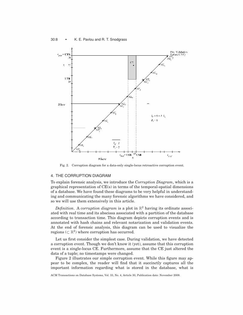
The CE just analyzed is termed a retroactive corruption event: a CE withlocus time tl appearing before the next to last validation event. Figure 3 illus-trates an introactive corruption event: a CE with a locus time tl appearing afterthe next to last validation event. In this figure, the corruption event occurredon day 22, as before, but altered data on day 21 (rather than day 16 in the previ-ous diagram). NE10 is the most recent validation success. Here, the corruptionregion is a trapezoid in the corruption diagram, rather than a rectangle, due tothe constraint mentioned earlier that a CE must be on or above the action line(tc ≥ tl ). This constraint is reflected in the definition of LTB.
It is worth mentioning here that these CEs are ones that only corrupt data.It is conceivable that a CE could alter the timestamp (transaction commit time)of a tuple. This creates two new independent types of CEs, termed postdatingor backdating CEs, depending on how the timestamp was altered. An analysisof timestamp corruption will be provided in Section 7.
ACM Transactions on Database Systems, Vol. 33, No. 4, Article 30, Publication date: November 2008.

Forensic Analysis of Database Tampering • 30:13
Fig. 3. Corruption diagram for a data-only single-locus introactive corruption event.
6. NOTARIZATION AND VALIDATION INTERVALS
The two corruption diagrams we have thus far examined assumed a notariza-tion interval of IN = 2 and validation interval of IV = 6. In this case, nota-rization occurs more frequently than validation and the two processes are inphase, with IV a multiple of IN . In such a scenario, we saw that the spatialuncertainty is determined by the notarization interval, and the temporal un-certainty by the validation interval. Hence we obtained tall, thin CE regions.One naturally asks, what about other cases?
Say notarization events occur at midnight every two days, as before, andvalidation events occur every three days, but at noon. So we might haveNE1 on Monday night, NE2 on Wednesday night, NE3 on Friday night,VE1 on Wednesday at noon, and VE2 on Saturday at noon. VE1 rehashesthe database up to Monday night and checks that linked hash value withthe digital notarization service. It would detect tampering prior to Mondaynight; tampering with a tl after Monday would not be detected by VE1. VE2
would hash through Friday night; tampering on Tuesday would then be de-tected. Hence we see that a nonaligned validation just delays detection oftampering. Simply speaking, one can validate only what one has previouslynotarized.
ACM Transactions on Database Systems, Vol. 33, No. 4, Article 30, Publication date: November 2008.
30:14 • K. E. Pavlou and R. T. Snodgrass
If the validation interval were shorter than the notarization interval, thatis IN = 2, IV = 1, say every day at midnight, then a validation on Tuesday atmidnight could again only check through Monday night.
Our conclusion is that the validation interval should be equal to or longerthan the notarization interval, should be a multiple of the notarization interval,and should be aligned, that is, validation should occur immediately after nota-rization. Thus we will speak of the validation factor V such that IV = V · IN .As long as this constraint is respected, it is possible to change V , or both IVand IN , as desired. This, however, will affect the size of the corruption regionand subsequently the cost of the forensic analysis algorithms, as emphasizedin Section 9.
7. ANALYZING TIMESTAMP CORRUPTION
The previous section considered a data-only corruption event, a CE that doesnot change timestamps in the tuples. There are two other kinds of corruptionevents with respect to timestamp corruption. In a backdating corruption event,a timestamp is changed to indicate a previous time/date with respect to theoriginal time in the tuple. We term the time a timestamp was backdated tothe backdating time, or tb. It is always the case that tb < tl . Similarly, a post-dating corruption event changes a timestamp to indicate a future time/datewith respect to the original commit time in the tuple, with the postdating time(tp) being the time a timestamp was postdated to. It is always the case thattl < tp. Combined with the previously introduced distinction of retroactive andintroactive, these considerations induce six specific corruption event types.
{Retroactive
Introactive
}×
⎧⎪⎪⎨⎪⎪⎩
Data-only
Backdating
Postdating
⎫⎪⎪⎬⎪⎪⎭
For backdating corruption events, we ask that the forensic analysis deter-mine, to the extent possible, when (tc), where (tl ), and to where (tb). Similarly,for postdating corruption events, we want to determine tc, tl , and tp. This isquite challenging given the only information we have, which is a single bit foreach query on the notarization service.
It bears mention that neither postdating nor backdating CEs involve move-ment of the actual tuple to a new location on disk. Instead, these CEs consistentirely of changing an insertion-date timestamp attribute. (We note in pass-ing that in some transaction-time storage organizations the tuples are stored incommit order. If an insertion date is changed during a corruption event, the factthat that tuple is out of order provides another clue, one that we don’t exploitin the algorithms proposed here.)
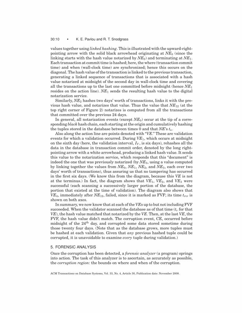
Figure 4 illustrates a retroactive postdating corruption event (denoted bythe forward-pointing arrow). On day 22, the timestamp of a tuple written onday 10 was changed to make it appear that that tuple was inserted on day 14(perhaps to avoid seeming that something happened on day 10). This tamperingwill be detected by VE4, which will set the lower and upper temporal boundsof the CE, shown in Figure 4 as LTB = 18 and UTB = 24. The Monochromatic
ACM Transactions on Database Systems, Vol. 33, No. 4, Article 30, Publication date: November 2008.

Forensic Analysis of Database Tampering • 30:15
Fig. 4. Corruption diagram for postdating and backdating corruption events.
Algorithm will then go back and rehash the database, querying with the no-tarization service at NE0, NE1, NE2, . . . . It will notice that NE4 is the mostrecent validation success, because the rehashed sequence will not contain thetampered tuple: its (altered) timestamp implies it was stored on day 14. Giventhat the query at NE4 succeeds and that at NE5 fails, the tampered data musthave been originally stored sometime during those two days, thus bounding tlto day 9 or day 10. This provides the corruption region shown as the left-shadedrectangle in the figure.
Since this is a postdating corruption event, tp, the date the data was alteredto, must be after the local time, tl . Unfortunately, all subsequent revalidations,from NE5 onward, will fail, then giving us absolutely no additional informationas to the value of tp. The “to” time is thus somewhere in the shaded trapezoidto the right of the corruption region. (We show this on the corruption diagramas a two-dimensional region, representing the uncertainty of tc and tp. Hencethe two shaded regions denote just three uncertainties, in tc, tl , and tp.)
Figure 4 also illustrates a retroactive backdating corruption event(backward-pointing arrow). On day 22, the timestamp of a tuple written on
ACM Transactions on Database Systems, Vol. 33, No. 4, Article 30, Publication date: November 2008.

30:16 • K. E. Pavlou and R. T. Snodgrass
day 14 was changed to make it appear that the tuple in question was insertedon day 10 (perhaps to imply something happened before it actually did). Thistampering will be detected by VE4, which will set the lower and upper tem-poral bounds of the CE (as in the postdating case). Going back and rehash-ing the data at NE0, NE1, . . . the Monochromatic Algorithm will compute thatNE4 is the most recent validation success. The rehashing up to NE5 will failto match its notarized value, because the rehashed sequence will erroneouslycontain the tampered tuple that was originally was stored on day 14. Giventhat the query at NE4 succeeds and that at NE5 fails, the new timestampmust be sometime within those two days, thus bounding tb to day 9 or day 10.The left-shaded rectangle in the figure illustrates the extent of the imprecisionof tb.
Since this is a backdating corruption event, the date the data was originallystored, tl , must be after the “to” time, tb. As with postdating CEs, all subse-quent revalidations, from NE5 onward, will fail, then giving us absolutely noadditional information as to the value of tl . The corruption region is thus theshaded trapezoid in the figure.
While we have illustrated backdating and postdating corruption events sepa-rately, the Monochromatic Algorithm is unable to differentiate these two kindsof events from each other, or from a data-only corruption event. Rather, thealgorithm identifies the RVS, the most recent validation success, and from thatputs a two-day bound on either tl or tb. Because the black link chains that arenotarized by NEs are cumulative, once one fails during a rehashing, all futureones will fail. Thus future NEs provide no additional information concerningthe corruption event.
To determine more information about the corruption event, we have littlechoice but to utilize to a greater extent the external notarization service. (Recallthat the notarization service is the only thing we can trust after an intrusion.)At the same time, it is important to not slow down regular processing. We’llshow how both are possible.
8. FORENSIC ANALYSIS ALGORITHMS
In this section we provide a uniform presentation and detailed analysis of foren-sic analysis algorithms. The algorithms presented are the original Monochro-matic Algorithm, the RGBY Algorithm, the Tiled Bitmap Algorithm [Pavlouand Snodgrass 2006b], and the a3D Algorithm. Each successive algorithm in-troduces additional chains during normal processing in order to achieve moredetailed results during forensic analysis. This comes at the increased expense ofmaintaining—hashing and validating—a growing number of hash chains. Weshow in Section 9 that the increased benefit in each case more than compensatesfor the increased cost.
The Monochromatic Algorithm uses only the cumulative (black) hash chainswe have seen so far, and as such it is the simplest algorithm in terms ofimplementation.
The RGBY Algorithm introduced here is an improvement of the original RGBAlgorithm [Pavlou and Snodgrass 2006a]. The main insight of the previously
ACM Transactions on Database Systems, Vol. 33, No. 4, Article 30, Publication date: November 2008.
Forensic Analysis of Database Tampering • 30:17
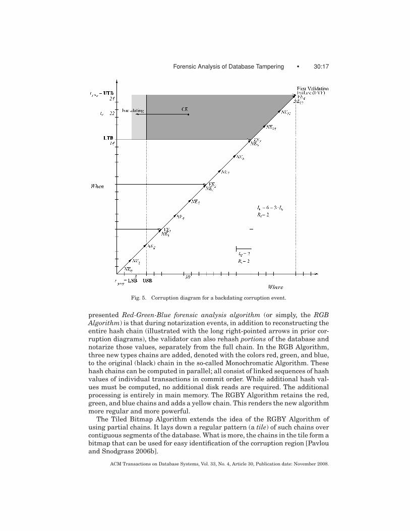
Fig. 5. Corruption diagram for a backdating corruption event.
presented Red-Green-Blue forensic analysis algorithm (or simply, the RGBAlgorithm) is that during notarization events, in addition to reconstructing theentire hash chain (illustrated with the long right-pointed arrows in prior cor-ruption diagrams), the validator can also rehash portions of the database andnotarize those values, separately from the full chain. In the RGB Algorithm,three new types chains are added, denoted with the colors red, green, and blue,to the original (black) chain in the so-called Monochromatic Algorithm. Thesehash chains can be computed in parallel; all consist of linked sequences of hashvalues of individual transactions in commit order. While additional hash val-ues must be computed, no additional disk reads are required. The additionalprocessing is entirely in main memory. The RGBY Algorithm retains the red,green, and blue chains and adds a yellow chain. This renders the new algorithmmore regular and more powerful.
The Tiled Bitmap Algorithm extends the idea of the RGBY Algorithm ofusing partial chains. It lays down a regular pattern (a tile) of such chains overcontiguous segments of the database. What is more, the chains in the tile form abitmap that can be used for easy identification of the corruption region [Pavlouand Snodgrass 2006b].
ACM Transactions on Database Systems, Vol. 33, No. 4, Article 30, Publication date: November 2008.
30:18 • K. E. Pavlou and R. T. Snodgrass
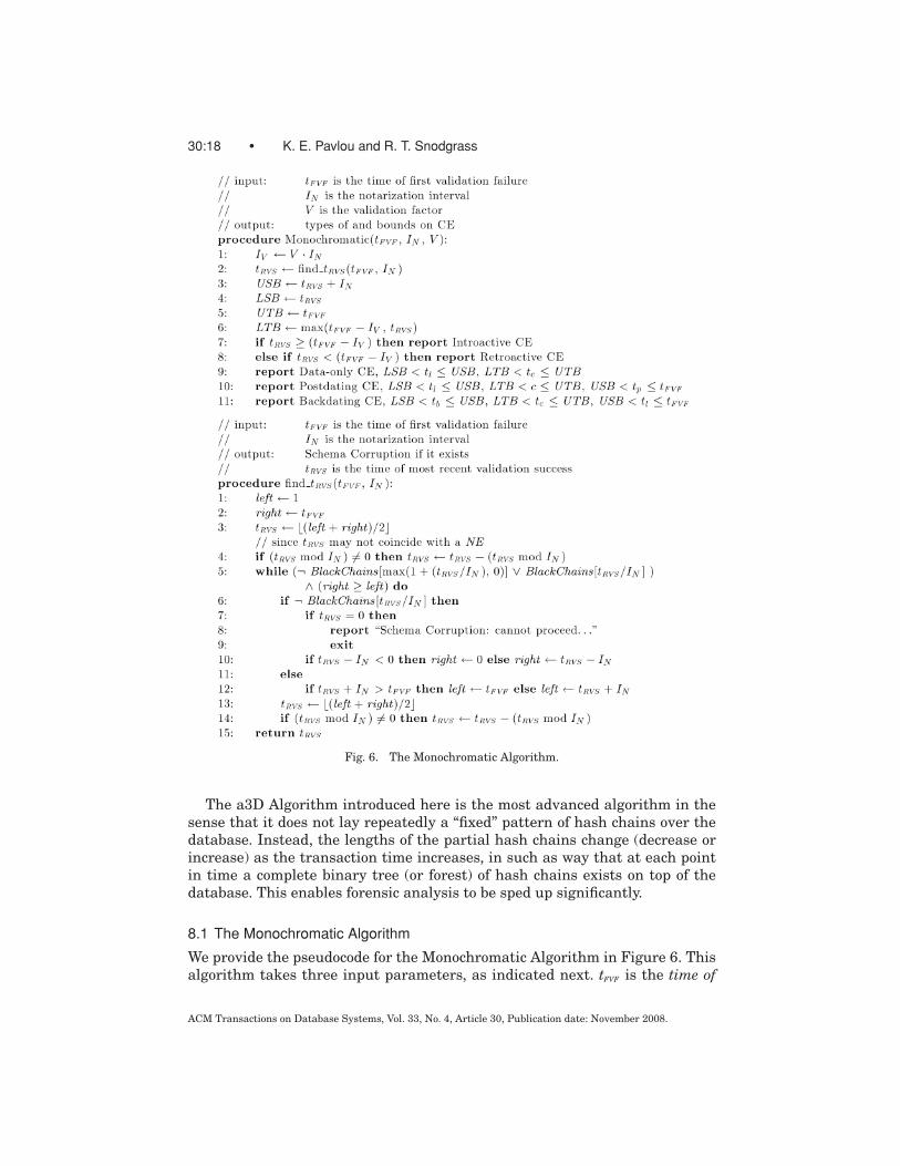
Fig. 6. The Monochromatic Algorithm.
The a3D Algorithm introduced here is the most advanced algorithm in thesense that it does not lay repeatedly a “fixed” pattern of hash chains over thedatabase. Instead, the lengths of the partial hash chains change (decrease orincrease) as the transaction time increases, in such as way that at each pointin time a complete binary tree (or forest) of hash chains exists on top of thedatabase. This enables forensic analysis to be sped up significantly.
8.1 The Monochromatic Algorithm
We provide the pseudocode for the Monochromatic Algorithm in Figure 6. Thisalgorithm takes three input parameters, as indicated next. tFVF is the time of
ACM Transactions on Database Systems, Vol. 33, No. 4, Article 30, Publication date: November 2008.

Forensic Analysis of Database Tampering • 30:19
first validation failure, that is, the time at which the corruption of the log isfirst detected. In every corruption diagram, tFVF coincides with the current time.IN is the notarization interval, while V, called the validation factor, is the ratioof the validation interval to the notarization interval (V = IV /IN , V ∈ N). Thealgorithm assumes that a single CE transpires in each example. The resolutionsfor the Monochromatic Algorithm are Rs = IN and Rt = IV = V · IN . (TheDBA can set the resolutions indirectly, by specifying IN and V .) Hence if a CEinvolving a timestamp transpires and tl and tp/tb are both within the same IN ,such a (backdating or postdating) corruption cannot be distinguished from adata-only CE, and hence it is treated as such.
The algorithm first identifies tRVS, the time of most recent validation success,and from that puts an IN bound on either tl or tb. Then depending on the valueof tRVS it distinguishes between introactive and retroactive CEs. It then reportsthe (where) bounds on tl and tp (or tb) of both data-only and timestamp CEs,since it cannot differentiate between the two. These bounds are given in termsof the upper spatial bound (USB) and the lower spatial bound (LSB). The timeinterval where time of corruption tc lies is bounded by the lower and uppertemporal bounds (LTB and UTB).
It is worth noting here that the points (tl , tc) and (tp, tc)—or (tb, tc)—must always share the same when-coordinate, since both refer to a single CE.The algorithm reports multiple possibilities for the CEs, since the algorithmcan’t differentiate between all the different types of corruption. Also, the boundsare given in a way that is readable and quite simple. The results are capturedby a system of linear inequalities whose solution conveys the extent of the cor-ruption region.
The find tRVS function, which is used on line 2 in the Monochromatic procedureof Figure 6, finds the time of most recent validation success by performingbinary search on the cumulative black chains. It revisits past notarizationsand, by validating them, it decides whether to recurse to the right or to the leftof the current chain.
In this algorithm we use an array BlackChains of Boolean values to store theresults of validation during forensic analysis. The Boolean results are indexedby the subscript of the notarization event considered: the result of validat-ing NEi is stored at index i, that is, BlackChains[i]. Since we do not wish toprecompute all this information, the validation results are computed lazily,that is, whenever needed. On line 7 we report only if there is schema corrup-tion and no other special checks are made in order to deal with this special caseof corruption.
Note that on lines 6 and 11 these are the only possibilities for the validationresults of the NEs in question. No other case ever arises, since the results ofthe validations of the cumulative black chains, considered from right to left,always follow a (single) change from false to true.
The running time of the Monochromatic Algorithm is dominated by the sim-ple binary search required to find tRVS. It ultimately depends on the numberof cumulative black hash chains maintained. Hence the running time of theMonochromatic Algorithm is O(lg(tFVF/IN )).
ACM Transactions on Database Systems, Vol. 33, No. 4, Article 30, Publication date: November 2008.

30:20 • K. E. Pavlou and R. T. Snodgrass
Fig. 7. Corruption diagram for the RGBY Algorithm.
8.2 The RGBY Algorithm
We now present an improved version of the RGB Algorithm that we call theRGBY Algorithm. RGBY has a more regular structure and avoids some of RGB’sambiguities. The RGBY chains are of the same types as in the original RGB Al-gorithm. The black cumulative chains are used in conjunction with new partialhash chains, that is, chains that do not extend all the way back to the originof the corruption diagram. Another difference is that these partial chains areevaluated and notarized during a validation scan of the entire database and,for this reason, they are shown running parallel to the Where axis (instead ofbeing on the action axis) in Figure 7. The introduction of the partial hash chainswill help us deal with more complex scenarios, for example, multiple data-onlyCEs or CEs involving timestamp corruption.
The partial hash chains in RGB are computed as follows. (We assumethroughout that the validation factor V = 2 and IN is a power of two.)
— for odd i the Red chain covers NE2·i−3 through NE2·i−1.
— for even i the Blue chain covers NE2·i−3 through NE2·i−1.
— for even i the Green chain covers NE2·i−2 through NE2·i.
ACM Transactions on Database Systems, Vol. 33, No. 4, Article 30, Publication date: November 2008.

Forensic Analysis of Database Tampering • 30:21
In this new algorithm we simply introduce a new Yellow chain, computed asfollows:
— for odd i the Yellow chain covers NE2·i−2 through NE2·i.
In Figure 7 the colors of the partial hash chains are denoted along the Whenaxis with the labels Red, Green, Blue, and Yellow (the figure is still in black andwhite). We use subscripts to differentiate between chains of the same color inthe corruption diagram. Each chain takes its subscript from the correspondingVE. In the pseudocode we use instead a two-dimensional array called Chain. Itis indexed as Chain[color, number], where number refers to the subscript of thechain, while color is an integer between 0 and 3 with the following meaning:
— if color = 0 then Chain refers to a Blue chain.
— if color = 1 then Chain refers to a Green chain.
— if color = 2 then Chain refers to a Red chain.
— if color = 3 then Chain refers to a Yellow chain.
We also introduce the following comparisons:
Chain[color1, number1] ≺ Chain[color2, number2] iff(number1 < number2) ∨ (number1 = number2 ∧ color1 < color2),
Chain[color1, number1] = Chain[color2, number2] iff(number1 = number2 ∧ color1 = color2).
The algorithm requires that V = 2. This is because the chains are dividedinto two groups: red/yellow, added at odd-numbered validation events, andblue/green, added at even-numbered validation events. Note that the find tRVS
routine from the Monochromatic Algorithm is used here. As with the Monochro-matic Algorithm, the spatial detection resolution is equal to the validation inter-val (Rs = IV ) and the temporal detection resolution is equal to the notarizationinterval (Rt = IN ).
In this algorithm (shown in Figure 8), as well as in all subsequent ones, in-stead of using an array BlackChains to store the Boolean values of the validationresults, as that used in find tRVS, we use a helper function called val check. Thisfunction takes a hash chain as a parameter and returns the Boolean result ofthe validation of that chain.
During the normal processing, the cumulative black hash chains are evalu-ated and notarized. During a VE, the entire database is scanned and validated,while the partial (colored) hash chains are evaluated and notarized.
On line 2 we initialize a set that accumulates all the corrupted granules(in this case, days). Line 3 computes tRVS and lines 4–7 set the temporal andspatial bounds of the oldest corruption. On lines 9–10, we compute what isthe most recent partial chain (lastChain), while on lines 11–13 we computethe rightmost chain covering the oldest corruption (currChain). In Figure 7 theoldest corruption is in the IN covering days 9 and 10, so currChain is Yellow3.The “while” loop on line 14 linearly scans all the partial chains to the right oftRVS, that is, from currChain to lastChain, and checks for the pattern . . .TFFT. . .
in order to identify the corrupted granules. To achieve this, the algorithm mustcheck the validation result of chainChain and its immediate successor. Lines
ACM Transactions on Database Systems, Vol. 33, No. 4, Article 30, Publication date: November 2008.
30:22 • K. E. Pavlou and R. T. Snodgrass
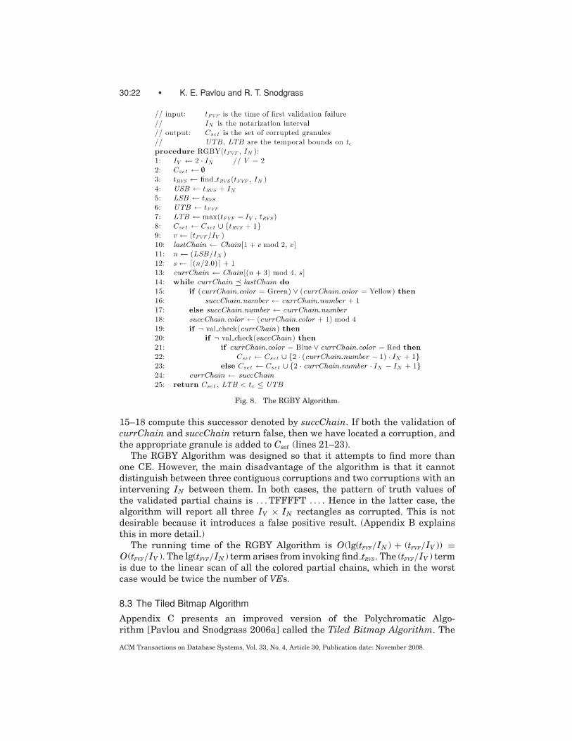
Fig. 8. The RGBY Algorithm.
15–18 compute this successor denoted by succChain. If both the validation ofcurrChain and succChain return false, then we have located a corruption, andthe appropriate granule is added to Cset (lines 21–23).
The RGBY Algorithm was designed so that it attempts to find more thanone CE. However, the main disadvantage of the algorithm is that it cannotdistinguish between three contiguous corruptions and two corruptions with anintervening IN between them. In both cases, the pattern of truth values ofthe validated partial chains is . . . TFFFFT . . . . Hence in the latter case, thealgorithm will report all three IV × IN rectangles as corrupted. This is notdesirable because it introduces a false positive result. (Appendix B explainsthis in more detail.)
The running time of the RGBY Algorithm is O(lg(tFVF/IN ) + (tFVF/IV )) =O(tFVF/IV ). The lg(tFVF/IN ) term arises from invoking find tRVS. The (tFVF/IV ) termis due to the linear scan of all the colored partial chains, which in the worstcase would be twice the number of VEs.
8.3 The Tiled Bitmap Algorithm
Appendix C presents an improved version of the Polychromatic Algo-rithm [Pavlou and Snodgrass 2006a] called the Tiled Bitmap Algorithm. The
ACM Transactions on Database Systems, Vol. 33, No. 4, Article 30, Publication date: November 2008.
Forensic Analysis of Database Tampering • 30:23
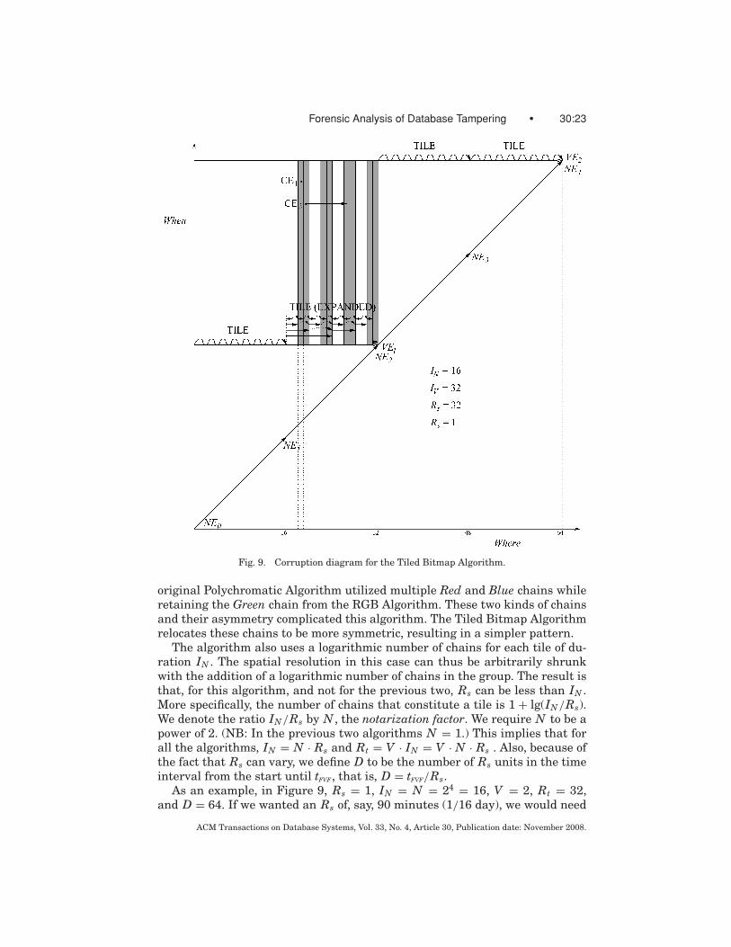
Fig. 9. Corruption diagram for the Tiled Bitmap Algorithm.
original Polychromatic Algorithm utilized multiple Red and Blue chains whileretaining the Green chain from the RGB Algorithm. These two kinds of chainsand their asymmetry complicated this algorithm. The Tiled Bitmap Algorithmrelocates these chains to be more symmetric, resulting in a simpler pattern.
The algorithm also uses a logarithmic number of chains for each tile of du-ration IN . The spatial resolution in this case can thus be arbitrarily shrunkwith the addition of a logarithmic number of chains in the group. The result isthat, for this algorithm, and not for the previous two, Rs can be less than IN .More specifically, the number of chains that constitute a tile is 1 + lg(IN/Rs).We denote the ratio IN/Rs by N , the notarization factor. We require N to be apower of 2. (NB: In the previous two algorithms N = 1.) This implies that forall the algorithms, IN = N · Rs and Rt = V · IN = V · N · Rs . Also, because ofthe fact that Rs can vary, we define D to be the number of Rs units in the timeinterval from the start until tFVF, that is, D = tFVF/Rs.
As an example, in Figure 9, Rs = 1, IN = N = 24 = 16, V = 2, Rt = 32,and D = 64. If we wanted an Rs of, say, 90 minutes (1/16 day), we would need
ACM Transactions on Database Systems, Vol. 33, No. 4, Article 30, Publication date: November 2008.

30:24 • K. E. Pavlou and R. T. Snodgrass
another four chains: 1 + lg(IN/Rs) = 1 + lg(16/ 116
) = 9. (Appendix C explainsthis figure in much more detail.)
In all of the algorithms presented thus far, discovering corruption (CEs orpostdating intervals) to the right of tRVS is achieved using a linear search thatvisits potentially all the hash chains in this particular interval. Due to thenature of these algorithms, this linear search is unavoidable. The Tiled Bitmapalgorithm reduces the size of the linear search by just iterating on the longestpartial chains (c(0)) that cover each tile. The running time of the Tiled BitmapAlgorithm is shown in Appendix C to be O(D).
In addition, the Tiled Bitmap Algorithm may handle multiple CEs but itpotentially overestimates the degree of corruption by returning the candidateset with granules which may or may not have suffered corruption (false pos-itives). The number of false positives in the Tiled Bitmap Algorithm could besignificantly higher than the number of false positives observed in the RGBYAlgorithm. Figure 9 shows that the Tiled Bitmap Algorithm will produce a can-didate set with the following granules (in this case, days): 19, 20, 23, 24, 27,28, 31, 32. The corruptions occur on granules 19, 20, and 27, while the rest arefalse positives. In order to overcome these limitations, we introduce the nextalgorithm.
8.4 The a3D Algorithm
We have seen that the existence of multi-locus CEs can be better handled bysummarizing the sites of corruption via candidate sets, instead of trying to findtheir precise nature. We proceed now to develop a new algorithm that avoidsthe limitations of all the previous algorithms and at the same time handles theexistence of multi-locus CEs successfully. We call this new algorithm the a3DAlgorithm for reasons that will become obvious when we analyze it. The a3D Al-gorithm is illustrated in Figure 10. Even though the corruption diagram showsonly VEs, it is implicit that these were preceded immediately by notarizationevents (not shown). The difference between the Tiled Bitmap Algorithm anda3D is that, in the latter, each chain is contiguous, that is, it has no gaps. Itwas the gaps that necessitated the introduction of the candidate sets. Figure 10shows that the corruption regions in the a3D Algorithm each correspond to asingle corruption. All existing corruptions at granules 4, 7, and 10 are identifiedwith no false positives. The difference between a3D and the other algorithmsis a slowly increasing number of chains at each validation. In Figure 10, thechains are named using letters B for the black cumulative chains, and P for thepartial chains. Observe that there is one diagonal full chain at VE1, and twopartial chains. VE2 has a full black chain (B2, with the subscript the day—Rsunit—of the validation event), retains the chains (P2,0,2 and P2,0,3), and addsa longer partial chain (P2,1,1). (We will explain these three subscripts shortly.)We add another chain at VE4 (P4,2,1) and another chain at VE8 (P8,3,1).
The a3D Algorithm assumes that, given an Rs, tFVF = 0, D = tFVF/Rs, andV = 1 (which implies that Rt = IN ).
The beauty of this algorithm is that it decides what chains to add based on thecurrent day/Rs unit. In this way, the number of chains increases dynamically,
ACM Transactions on Database Systems, Vol. 33, No. 4, Article 30, Publication date: November 2008.

Forensic Analysis of Database Tampering • 30:25
Fig. 10. Corruption diagram for the a3D Algorithm.
which allows us to perform binary search in order to locate the corruption. Ifwe dissociate the decision of how many chains to add from the current day, thenwe are forced to repeat a certain fixed pattern of hash chains, which results inthe drawbacks seen in the Tiled Bitmap Algorithm.
During normal processing, the algorithm adds partial hash chains (shownwith white-tipped arrows). These partial chains are labeled as P with threesubscripts. The first subscript is the number m of the current VE, such as P4,2,1
added at VE4. The second subscript, level, identifies the (zero-based) verticalposition of the chain P within a group of chains added at VEm. This subscriptalso provides the length of the partial chain as 2level. For example, chain P4,2,1
has length 22 = 4. The final subscript, comp (for component), determines thehorizontal position of the chain: all chains within a certain level have a positioncomp that ranges from 0 to 2level−1. For example, hash chain P4,2,1 is the secondchain at level 2. The first chain at level 2 is P2,2,0, which just happens to be theblack chain B2; the third chain at this level is P6,2,2; and the fourth chain isP8,2,3.
The addition of partial hash chains allows the algorithm to perform abottom-up creation of a binary tree whose nodes represent the hash chains (seeFigure 11). Depending on when the CE transpires, there maybe nodes missingfrom the complete tree, so in reality we have multiple binary trees that aresubtrees of the next complete tree. In Figure 11, the nodes/chains missing arethose in the shaded region, while there are three complete subtrees each rootedat B4 = P4,3,0, P6,2,2, and P7,1,6, respectively.
ACM Transactions on Database Systems, Vol. 33, No. 4, Article 30, Publication date: November 2008.

30:26 • K. E. Pavlou and R. T. Snodgrass
Fig. 11. The a3D Algorithm performs a bottom-up creation of a binary tree.
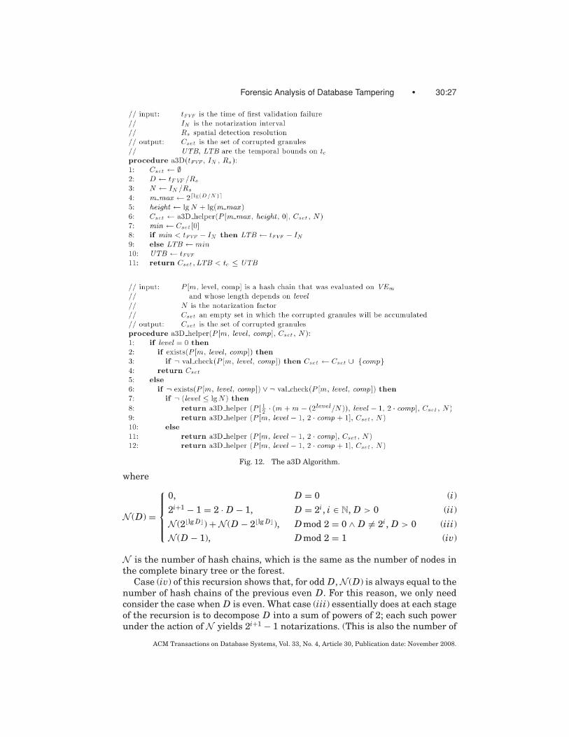
The a3D Algorithm is given in Figure 12. Note that when val check is calledwith a hash chain P [m, level, comp] for whom m is a power of 2, level ≥ lg(N ),and comp = 0, these chains are actually black chains whose validation resultcan be obtained through BlackChains[m]. All black chains appear only on theleftmost path from the root to the leftmost child; however, not all chains on thispath are black.
The a3D function evaluates the height of the complete tree, regardless ofwhether we have a single tree or a forest (line 5). Then it calls the recursivea3D helper function, which performs the actual search. In the recursive part ofa3D helper, the function calls itself (lines 8–9, 11–12) with the appropriate hash(sub-)chain only if the current chain does not exist or evaluates to false (line 6).In this case, we are relying on short-circuit Boolean evaluation for correctness.All of the compromised granules are accumulated into Cset .
The running time of the algorithm is dominated by the successive calls tothe recursive function a3D helper. The worst-case running time is captured bythe recursion T (D) = 2 · T (D/2) + O(1), that is, we have to recurse to both theleft and right children. The solution to this recursion gives us T (D) = �(D),so the algorithm is linear in the number of Rs units. In the best case, thealgorithm recurses on only one of the two children, and thus the running time isO(lg D).
The algorithm takes its name from the fact that, for a given D, the algorithmmakes in the worst case 3·D number of notarization contacts, as in the following:
Total Number of Notarizations = number of chains in tree+ number of black chains not in tree
= N (D)
+ D/N − (1 + lg(D/N )�) (1)
ACM Transactions on Database Systems, Vol. 33, No. 4, Article 30, Publication date: November 2008.
Forensic Analysis of Database Tampering • 30:27
Fig. 12. The a3D Algorithm.
where
N (D) =
⎧⎪⎪⎪⎨⎪⎪⎪⎩
0, D = 0 (i)
2i+1 − 1 = 2 · D − 1, D = 2i, i ∈ N, D > 0 (ii)
N (2lg D�) + N (D − 2lg D�), D mod 2 = 0 ∧ D = 2i, D > 0 (iii)N (D − 1), D mod 2 = 1 (iv)
N is the number of hash chains, which is the same as the number of nodes inthe complete binary tree or the forest.
Case (iv) of this recursion shows that, for odd D, N (D) is always equal to thenumber of hash chains of the previous even D. For this reason, we only needconsider the case when D is even. What case (iii) essentially does at each stageof the recursion is to decompose D into a sum of powers of 2; each such powerunder the action of N yields 2i+1 − 1 notarizations. (This is also the number of
ACM Transactions on Database Systems, Vol. 33, No. 4, Article 30, Publication date: November 2008.
30:28 • K. E. Pavlou and R. T. Snodgrass
nodes in the subtree of height i.) Thus to evaluate this recurrence we examinethe binary representation of D. Each position in the binary representationwhere there is a ‘1’ corresponds to a power of 2 with decimal value 2i. Summingthe results of each one of these decimal values under the action of N givesthe desired solution to N (D). This solution can be captured mathematicallyusing Iverson brackets [Graham et al. 2004, p. 24] (here, & is a bit-wise ANDoperation):
N (D) =lg D�∑i=0
(2i+1 − 1) · [D&2i = 0].
The total number of notarizations is bounded above by the number 3 · D. Thisloose bound can be derived by simply assuming that the initial value of D is apower of 2. Assuming also that the complete binary tree has height H = lg D,then
Total Number of Notarizations ≤ 2 · D − 1 + D/N − (1 + lg(D/N )�)
< 2 · D + D/N minimum value of N = 1
≤ 3 · D.
8.5 Summary
We have presented four forensic analysis algorithms: Monochromatic, RGBY,Tiled Bitmap, and a3D.
Assuming worst case scenarios, the running time of the Monochromatic Al-gorithm is O(lg D); for the rest it is O(D). Each of these algorithms managesthe trade-off between effort during normal processing and effort during foren-sic analysis; the algorithms differ in the precision of their forensic analysis.So, while the Monochromatic Algorithm has the fastest running time, it offersno information beyond the approximate location of the earliest corruption. Theother algorithms work harder, but also provide more precise forensic informa-tion. In order to more comprehensively compare these algorithms, we desire tocapture this tradeoff and resulting precision in a single measure.
9. FORENSIC COST
We define the forensic cost as a function of D (expressed as the number of Rsunits), N , the notarization factor (with IN = N · Rs), V , the validation factor(with V = IV /IN ), and κ, the number of corruption sites (the total number of tl ’s,tb’s, and tp’s). A corruption site differs from a CE because a single timestampCE has two corruption sites.
FC(D, N , V , κ) = α · NormalProcessing(D, N , V )
+ β · ForensicAnalysis(D, N , V , κ)
+ γ · AreaP (D, N , V , κ) + δ · AreaU (D, N , V , κ)
Forensic cost is a sum of four components, each representing a cost that wewould like a forensic analysis algorithm to minimize, and each weighted by aseparate constant factor: α, β, γ , and δ. The first component, NormalProcessing,
ACM Transactions on Database Systems, Vol. 33, No. 4, Article 30, Publication date: November 2008.

Forensic Analysis of Database Tampering • 30:29
is the number of notarizations and validations made during normal processingin a span of D days. The second component, ForensicAnalysis, is the cost of foren-sic analysis in terms of the number of validations made by the algorithm to yielda result. Note that this is different from the running time of the algorithm. Therationale behind this quantity is that each notarization or validation involvesan interaction with the external digital notarization service, which costs realmoney.
The third and fourth components informally indicate the manual labor re-quired after automatic forensic analysis to identify exactly where and whenthe corruption happened. This manual labor is very roughly proportional to theuncertainty of the information returned by the forensic analysis algorithm. Itturns out that there are two kinds of uncertainties, formalized as different ar-eas (to be described shortly). That these components have different units thanthe first two components is accommodated by the weights.
In order to make the definition of forensic cost applicable to multiple corrup-tion events, we need to distinguish between three regions within the corruptiondiagram. These different areas are the result of the forensic analysis algorithmidentifying the corrupted granules. This distinction is based on the informationcontent of each type.
— AreaP or corruption positive area is the area of the region in which the foren-sic algorithm has established that corruption has definitively occurred.
— AreaU or corruption unknown area is the area of the region in which we don’tknow if or where a corruption has occurred.
— AreaN or corruption negative area is the area of the region in which theforensic algorithm has established that no corruption has occurred.
Each corruption site is associated with these three types of regions of varyingarea. More specifically, each site induces a partition of the horizontal trape-zoid bound by the latest validation interval into three types of forensic area.Figure 13 shows this for a specific example of the RGBY Algorithm with two cor-ruption events (CE1, CE2) and three corruption sites (κ = 3). For each corrup-tion site, the sum of the areas, denoted by TotalArea = AreaP + AreaU + AreaN ,corresponds to the horizontal trapezoid as shown. Hence TotalArea = (V · N ) ·(D − (1/2) · V · N ). Moreover, the forensic cost is a function of the number ofcorruption sites κ, each associated with the three areas AreaP , AreaU , AreaN .Hence in evaluating the forensic cost of a particular algorithm, we have to com-pute AreaP and AreaU for all κ, for example, AreaP (D, N , V , κ) = ∑
κ AreaP .The stronger the algorithm, the less costly it is, with smaller AreaP and AreaU .It is also desirable that AreaN is large but, since TotalArea is constant, this isachieved automatically by minimizing AreaP and AreaU .
We now proceed to compute the forensic cost of our algorithms. We ignorethe weights, since these constant factors will not be relevant when we use ordernotation.
9.1 The Monochromatic Algorithm
In the Monochromatic Algorithm, the spatial detection resolution (Rs) is thenotarization interval, IN , that is, N = 1. Recall that the Monochromatic
ACM Transactions on Database Systems, Vol. 33, No. 4, Article 30, Publication date: November 2008.

30:30 • K. E. Pavlou and R. T. Snodgrass
Fig. 13. Three types of forensic area for RGBY and κ = 3.
Algorithm can only detect a single corruption site, even though there couldbe κ of them in a single corruption diagram.
NormalProcessingmono = Number of Notarizations+ Number of Validations
= D + D/V
In forensic analysis calculations, we require D to be a multiple of V becausetFVF is a multiple of IV and only at that time instant can the forensic analysisphase start. ForensicAnalysismono = 2 · lg D, since tRVS is found via binary searchon the black chains; the factor of two is because a pair of contiguous chains mustbe consulted to determine which direction to continue the search.
For the detected corruption site, AreaP has a different shape depending onthe position of the corruption site. As the corruption site moves from left toright (from earlier days to later days), the shape of the region changes fromrectangular, to trapezoidal, and finally, to triangular. However, since we aredealing with worst-case scenario, the upper bound of AreaP is V · N 2 = V .Figure 14 shows such a worst-case distribution of κ corruption sites and howeach site partitions the horizontal trapezoid into different forensic areas. Inthe worst-case, the corruption detected occurs within the first IN , which makesAreaP = 0 of all other corruption sites because they cannot be detected. This
ACM Transactions on Database Systems, Vol. 33, No. 4, Article 30, Publication date: November 2008.

Forensic Analysis of Database Tampering • 30:31
Fig. 14. Three types of forensic area for Monochromatic and κ corruption sites.
Table II. The Forensic Areas for 1 ≤ κ ≤ D Corruption Sites
(Monochromatic)
# Corruption Sites
(1 ≤ κ ≤ D)AreaP AreaU AreaN
1 V 0 TotalArea − V
2 0 TotalArea − V V
.
.
....
.
.
....
κ 0 TotalArea − V V
results in:
AreaU = (κ − 1) · (TotalArea − V )
= (κ − 1) · [V · (D − (1/2) · V ) − V ]
= (κ − 1) · V · (D − (1/2) · V − 1).
as shown in Table II.Hence the forensic cost for the Monochromatic Algorithm is as follows:
FCmono(D, IN , V , κ) = (D + D/V + 2 · lg D)
+(
V +κ∑
i=2
(TotalArea − V )).
ACM Transactions on Database Systems, Vol. 33, No. 4, Article 30, Publication date: November 2008.
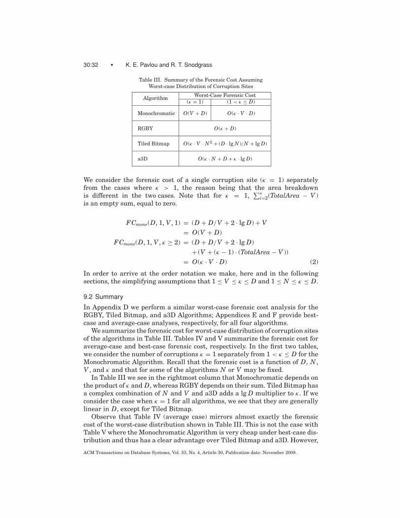
30:32 • K. E. Pavlou and R. T. Snodgrass
Table III. Summary of the Forensic Cost Assuming
Worst-case Distribution of Corruption Sites
Worst-Case Forensic CostAlgorithm
(κ = 1) (1 < κ ≤ D)
Monochromatic O(V + D) O(κ · V · D)
RGBY O(κ + D)
Tiled Bitmap O(κ · V · N2 + (D · lg N )/N + lg D)
a3D O(κ · N + D + κ · lg D)
We consider the forensic cost of a single corruption site (κ = 1) separatelyfrom the cases where κ > 1, the reason being that the area breakdownis different in the two cases. Note that for κ = 1,
∑κi=2(TotalArea − V )
is an empty sum, equal to zero.
FCmono(D, 1, V , 1) = (D + D/V + 2 · lg D) + V= O(V + D)
FCmono(D, 1, V , κ ≥ 2) = (D + D/V + 2 · lg D)
+ (V + (κ − 1) · (TotalArea − V ))
= O(κ · V · D) (2)
In order to arrive at the order notation we make, here and in the followingsections, the simplifying assumptions that 1 ≤ V ≤ κ ≤ D and 1 ≤ N ≤ κ ≤ D.
9.2 Summary
In Appendix D we perform a similar worst-case forensic cost analysis for theRGBY, Tiled Bitmap, and a3D Algorithms; Appendices E and F provide best-case and average-case analyses, respectively, for all four algorithms.
We summarize the forensic cost for worst-case distribution of corruption sitesof the algorithms in Table III. Tables IV and V summarize the forensic cost foraverage-case and best-case forensic cost, respectively. In the first two tables,we consider the number of corruptions κ = 1 separately from 1 < κ ≤ D for theMonochromatic Algorithm. Recall that the forensic cost is a function of D, N ,V , and κ and that for some of the algorithms N or V may be fixed.
In Table III we see in the rightmost column that Monochromatic depends onthe product of κ and D, whereas RGBY depends on their sum. Tiled Bitmap hasa complex combination of N and V and a3D adds a lg D multiplier to κ. If weconsider the case when κ = 1 for all algorithms, we see that they are generallylinear in D, except for Tiled Bitmap.
Observe that Table IV (average case) mirrors almost exactly the forensiccost of the worst-case distribution shown in Table III. This is not the case withTable V where the Monochromatic Algorithm is very cheap under best-case dis-tribution and thus has a clear advantage over Tiled Bitmap and a3D. However,
ACM Transactions on Database Systems, Vol. 33, No. 4, Article 30, Publication date: November 2008.
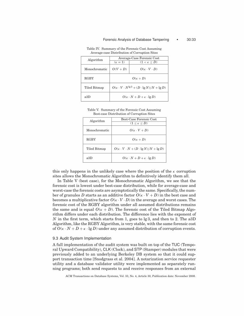
Forensic Analysis of Database Tampering • 30:33
Table IV. Summary of the Forensic Cost Assuming
Average-case Distribution of Corruption Sites
Average-Case Forensic CostAlgorithm
(κ = 1) (1 < κ ≤ D)
Monochromatic O(V + D) O(κ · V · D)
RGBY O(κ + D)
Tiled Bitmap O(κ · V · N lg 3 + (D · lg N )/N + lg D)
a3D O(κ · N + D + κ · lg D)
Table V. Summary of the Forensic Cost Assuming
Best-case Distribution of Corruption Sites
Best-Case Forensic CostAlgorithm
(1 ≤ κ ≤ D)
Monochromatic O(κ · V + D)
RGBY O(κ + D)
Tiled Bitmap O(κ · V · N + (D · lg N )/N + lg D)
a3D O(κ · N + D + κ · lg D)
this only happens in the unlikely case where the position of the κ corruptionsites allows the Monochromatic Algorithm to definitively identify them all.
In Table V (best case), for the Monochromatic Algorithm, we see that theforensic cost is lowest under best-case distribution, while for average-case andworst-case the forensic costs are asymptotically the same. Specifically, the num-ber of granules D starts as an additive factor O(κ · V + D) in the best case andbecomes a multiplicative factor O(κ · V · D) in the average and worst cases. Theforensic cost of the RGBY algorithm under all assumed distributions remainsthe same and is equal O(κ + D). The forensic cost of the Tiled Bitmap Algo-rithm differs under each distribution. The difference lies with the exponent ofN in the first term, which starts from 1, goes to lg 3, and then to 2. The a3DAlgorithm, like the RGBY Algorithm, is very stable, with the same forensic costof O(κ · N + D + κ · lg D) under any assumed distribution of corruption events.
9.3 Audit System Implementation
A full implementation of the audit system was built on top of the TUC (Tempo-ral Upward Compatibility), CLK (Clock), and STP (Stamper) modules that werepreviously added to an underlying Berkeley DB system so that it could sup-port transaction time [Snodgrass et al. 2004]. A notarization service requesterutility and a database validator utility were implemented as separately run-ning programs; both send requests to and receive responses from an external
ACM Transactions on Database Systems, Vol. 33, No. 4, Article 30, Publication date: November 2008.

30:34 • K. E. Pavlou and R. T. Snodgrass
digital notarization service, in this case Surety. The existence of the audit sys-tem imposed a 15% increase in time in the worst case when tuples are suf-ficiently small (10 bytes). The impact on time when record size and recordnumber were larger was even less than 15%. Hence the overhead for runtimehashing is small. The Monochromatic forensic analysis algorithm has been in-corporated into this system, and the rest of the algorithms are in the process ofbeing incorporated. We can make the following observations. We have an ideaof what the overhead is for the Monochromatic Algorithm because the normalprocessing part was evaluated before [Snodgrass et al. 2004]; the only part thatis missing is the forensic analysis phase, which revalidates past hash chains.All algorithms have the same number of I/O operations (and hence performancein terms of time) as the Monochromatic for the normal processing phase, sincefor all algorithms the database is scanned entirely only during validations.
9.4 Illustrating and Validating the Forensic Cost
We have implemented the Monochromatic, RGBY, Tiled Bitmap, and a3D Algo-rithms in C. The entire implementation is approximately 1480 lines long and thesource code is available at http://www.cs.arizona.edu/projects/tau/tbdb/.The forensic cost has been validated experimentally by inserting counters inthe appropriate places in the code. More specifically, the forensic cost and itsnormal processing component have been validated for values 1 ≤ D ≤ 256 and1 ≤ κ ≤ 256 as shown in Figures 15, 16, and 17.
To examine the effects of the various parameters on the theoretical cost, weprovide graphs showing the growth of forensic cost against these parameters.These are drawn on the same set of axes as the graphs derived experimentally.In all graphs, we have uniformly used D = 256 and Rs = 1. For the Monochro-matic Algorithm, N is required to be 1, so IN = 1, and we also set V = 8. Forthe RGBY Algorithm, N is also required to be 1 and V is required to be 2, so thisdictates Rt = 2. For the Tiled Bitmap Algorithm, we set N = 8, which impliesfour chains, and we also set V = 1. For the a3D Algorithm, we similarly setN = 8 and V = 1. All algorithms have Rt = 8 except for RGBY. The settingsused in the experimental validation are summarized in Table VI.
Rather than using the cost formulas in order notation to create the graphs,we used the more involved (and more accurate) cost functions derived foreach algorithm: equation (2) in Section 9.1 for the Monochromatic Algorithm,equation (3) in Appendix D.1 for the RGBY Algorithm, and equation (4) in Ap-pendix D.2 for the Tiled Bitmap Algorithm. For the a3D Algorithm we usedthe even more precise recursive formula equation (5) in Appendix D.3 to cal-culate the cost of normal processing instead of the one shown within (6) inAppendix D.3. Also, for values of D that are not a multiple of V · IN we usethe largest multiple of V · IN less than D to calculate the cost of the forensicanalysis stage.
Note that all cost plots show both the predicted forensic cost (denoted by“(P)” in the plot legend) and the actual forensic cost values (denoted by “(A)” inthe plot legend). The different types of symbols on the curves were added forclarity and correspond to a subset of the actual data points.
ACM Transactions on Database Systems, Vol. 33, No. 4, Article 30, Publication date: November 2008.

Forensic Analysis of Database Tampering • 30:35
Fig. 15. Forensic cost against κ for D = 256.
We start by examining the growth of forensic cost of the algorithms against κ,as shown in the graphs in Figure 15. Figure 15(a) shows how the forensic costincreases with κ. Most of the predicted forensic costs are very close to theactual values and in these cases (e.g., a3D algorithm) the two lines overlap.Figure 15(b) is a magnification of the region in Figure 15(a) where κ takes val-ues between 1 and 40. The cheapest algorithm for κ = D is RGBY, while themost expensive is Monochromatic. Observe in Figure 15(b) that for κ = 1 the
ACM Transactions on Database Systems, Vol. 33, No. 4, Article 30, Publication date: November 2008.

30:36 • K. E. Pavlou and R. T. Snodgrass
Fig. 16. Forensic cost against D for κ = 1 and κ = 2.
costs of Monochromatic and Tiled Bitmap are comparable and have the lowestvalue of all other algorithms.
Even more interestingly, the RGBY algorithm starts off as being the mostexpensive algorithm and then becomes the cheapest. This can be explained byobserving that ambiguity in the corruption region (large AreaU for κ > 1) in-creases the cost of the Monochromatic Algorithm. The Tiled Bitmap Algorithmsuffers considerably from false positives (for every true corruption site thereexist N − 1 false positives) On the other hand the comparison of a3D to RGBY
ACM Transactions on Database Systems, Vol. 33, No. 4, Article 30, Publication date: November 2008.

Forensic Analysis of Database Tampering • 30:37
Fig. 17. Cost of Normal Processing against D.
Table VI. Settings Used in Experimental Validation of Forensic
Cost Assuming Worst-case Distribution of Corruption Sites (values
in bold are non-configurable)
Algorithm
Parameters Monochromatic RGBY Tiled Bitmap a3D
Rs 1 1 1 1
N 1 1 8 8
V 8 2 1 1D 256 256 256 256
is more subtle. a3D starts below RGBY but eventually becomes more expensive.The reason is that, initially, RGBY has to linearly scan all its partial chains,whereas a3D does not (this happens only for D/2 ≤ κ ≤ D). However, the over-head of validating the a3D tree outweighs the impact of the presence of falsepositives produced by RGBY.
Figure 16 shows how the forensic cost increases with time D for differentnumbers of corruption sites, namely, κ = 1, and κ = 2. As expected for κ = 1(Figure 16(a)), the Monochromatic Algorithm has the lowest forensic cost forroughly the first half of the range of values of D. For the second half, the TiledBitmap Algorithm becomes the cheapest because it is able to definitively iden-tify all the corruption negative areas through a logarithmic number of chains.
When κ = 2 the Tiled Bitmap Algorithm is cheapest, as shown in Fig-ure 16(b). This is because Tiled Bitmap need only identify a single additionaltile, whereas a3D (the second cheapest algorithm) has to process an entire sub-tree of maximal height. Also, for this value of κ the Monochromatic Algorithmbecomes the most expensive algorithm.
ACM Transactions on Database Systems, Vol. 33, No. 4, Article 30, Publication date: November 2008.

30:38 • K. E. Pavlou and R. T. Snodgrass
Table VII. Sample Forensic Costs for the Four Implemented
Algorithms
Forensic Cost Monochromatic RGBY Tiled Bitmap a3D
Predicted 512352 1934 17610 3128
Actual 512354 1935 16714 3134
Finally, Figure 17 shows how the cost of only the normal processing phasevaries with the number of days D. Note that this cost is independent of κ. Herewe see clearly that the most expensive normal processing phase belongs to theRGBY Algorithm. a3D is the next most expensive algorithm, while Tiled Bitmapis the cheapest in terms of normal processing. This suggests that shifting thecost/amount of work done to the normal processing phase may not always payoff during forensic analysis.
Table VII shows the predicted and actual forensic costs for the four imple-mented algorithms when D = κ = 256. The two values in each of the fourcases differ by about 6% for Tiled Bitmap; for the other three, the actual andpredicted were nearly identical.
10. A LOWER BOUND FOR FORENSIC COST
We wish to derive a realistic lower bound for the Forensic Cost measure in termsof κ corruption sites, validation factor V , notarization interval IN , and D daysbefore the corruption is first detected.
The optimal value for AreaU is 0, whereas the optimal value for AreaP isκ · V · IN ·w, where w is the width and V · IN = IV is the height of the rectanglein which the corruption site is located.
Keep in mind that these algorithms do not aim at reducing the tc uncertainty.The size of the uncertainty of this temporal dimension depends solely on thesize of the validation interval (IV ) and therefore it can be reduced if and onlyif IV is reduced. No other factor involving external notarization can have anyimpact on it. This is due to the fact that the tc uncertainty is bounded aboveby the current time—the time the CE was discovered—and is also boundedbelow by the last time we checked the database, the last VE time. This isby definition the validation interval. Any new strategies introduced that arepurely native to the system cannot be trusted and thus violate the workingpremise of this approach: no extra assumptions should be made about thesystem.
To obtain bounds on the Normal Processing and Forensic Analysis phases, westart with a rather optimistic scenario. Suppose that we had a priori knowledge(both when and where) of the exact κ granules to be corrupted in the future.Then the optimal algorithm would notarize κ hash chains of length one, eachcovering the granule to be corrupted. Similarly, the forensic analysis wouldvalidate those κ hash chains and that would find all corruption sites, eachbounded by a rectangle of height V · IN and width w = 1 granule (where agranule is a unit of Rs). Thus a lower bound would be
FClower bound1= (κ + κ) + κ · V · IN · 1 = 2 · κ + κ · V · IN .
ACM Transactions on Database Systems, Vol. 33, No. 4, Article 30, Publication date: November 2008.

Forensic Analysis of Database Tampering • 30:39
However, we do not feel it is fair to tax our algorithms with the burden ofprecognition. While we still assume that κ and D are known, we have no a prioriknowledge of where the corruption sites are going to occur (within D). Giventhis information, we seek to find the optimal value for n ≥ κ, the number of no-tarizations during normal processing. The cost of Normal Processing = n, whilethe cost of Forensic Analysis = κ · lg n. This is because, for every κ, we must per-form binary search in order to locate it. The width w for AreaP is D/2n becauseeach notarization provides a single bit of information in the where dimension.
FClower bound2= (n + κ · lg n)
+ κ · V · IN · D/2n
If we assume that the width w can take a minimum value of w = 1, then itfollows that n = lg D. If we substitute this value of n into the previous FCexpression, we get:
FClower bound2= (lg D + κ · lg lg D) + κ · V · IN .
This lower bound makes fewer assumptions about the information availableand therefore FClower bound1
≤ FClower bound2. Our final lower bound is:
FClower bound = κ · V · IN + κ · lg lg D + lg D , κ ≤ D= O(κ · V · N + lg D).
Table VIII compares this lower bound with the worst-case forensic cost of ouralgorithms, characterized for “small κ” and “large κ.” In particular, we elimi-nate κ by assuming it is either equal to O(1) or O(D), respectively. Note thatfor the Monochromatic Algorithm, if κ = O(1), we assume that V D, thussimplifying the cost from O(V +D) to O(D). Tables IX and X repeat this compar-ison with average- and best-case forensic costs derived in Appendices E and F.The lower bound across all three tables is the same because the only way forthe lower bound to decrease in the best-case and average-case analysis is for thebinary search to be faster during forensic analysis. All other components areessential, that is, n notarizations are required, and the width w must equal 1.Binary search in the best-case takes O(1), eliminating the lg lg D factor, whichin asymptotic notation is irrelevant. In the average-case forensic cost, the av-erage running time of binary search is O(lg n) so the lower bound remains thesame. Hence there is only the notion of a single lower bound.For best-case forensic cost, the Monochromatic algorithm (which requires N =1) and the RGBY algorithm (which requires N = 1 and V = 2) are optimalfor large κ. Observe also that the asymptotic forensic cost of both the RGBYAlgorithm and that of the a3D Algorithm (which requires V = 1) for all possiblecases (worst, best, average) is optimal for large κ and is close to optimal forsmall κ.
11. RECOMMENDATIONS
Given the forensic cost formulæ and the insights from the previous sections,our recommendation is that it is best to provide users with three algorithms:
ACM Transactions on Database Systems, Vol. 33, No. 4, Article 30, Publication date: November 2008.

30:40 • K. E. Pavlou and R. T. Snodgrass
Table VIII. Worst-case Forensic Cost and Lower Bound
Worst-Case Forensic CostAlgorithm
Small κ (κ = O(1)) Large κ (κ = O(D))
Monochromatic O(D) O(V · D2)
RGBY O(D)
Tiled Bitmap O(V · N2 + (D · lg N )/N + lg D) O(V · N2 · D)
a3D O(N + D) O(N · D)
Lower Bound O(V · N + lg D) O(V · N · D)
Table IX. Average-case Forensic Cost and Lower Bound
Average-Case Forensic CostAlgorithm
Small κ (κ = O(1)) Large κ (κ = O(D))
Monochromatic O(D) O(V · D2)
RGBY O(D)
Tiled Bitmap O(V · N lg 3 + (D · lg N )/N + lg D) O(V · N lg 3 · D)
a3D O(N + D) O(N · D)
Lower Bound O(V · N + lg D) O(V · N · D)
Table X. Best-case Forensic Cost and Lower Bound
Best-Case Forensic CostAlgorithm
Small κ (κ = O(1)) Large κ (κ = O(D))
Monochromatic O(D) O(V · D)
RGBY O(D)
Tiled Bitmap O(V · N + (D · lg N )/N + lg D) O(V · N · D)
a3D O(N + D) O(N · D)
Lower Bound O(V · N + lg D) O(V · N · D)
Monochromatic, a3D and, depending on the application requirements, RGBY orTiled Bitmap. The reason for considering RGBY and Tiled Bitmap as optionalis that both these algorithms, unlike the Monochromatic and a3D, suffer fromfalse positives. The RGBY Algorithm has the same optimal characteristics asa3D and is the cheapest when a large number of corruptions is expected. On
ACM Transactions on Database Systems, Vol. 33, No. 4, Article 30, Publication date: November 2008.
Forensic Analysis of Database Tampering • 30:41
the other hand, the Tiled Bitmap Algorithm has the lowest forensic cost in thelong term for a fixed small number of corruptions but suffers from more falsepositives than RGBY, which translates into more human effort when trying topinpoint the exact corruptions at a later stage. The Tiled Bitmap Algorithm isalso indicated when efficiency during normal processing is critical.
If only two algorithms are to be used, then both Monochromatic and a3Dshould be implemented. If only one algorithm is needed, the choice would beagain between the Monochromatic and a3D Algorithms. The MonochromaticAlgorithm is by far the simplest one to implement and it is best-suited forcases when multiple corruptions are not anticipated or when only the earliestcorruption is desired. The a3D Algorithm is the second easiest algorithm toimplement and it is the only algorithm that exhibits all three of the most desir-able characteristics: (i) it identifies multiple corruptions, (ii) it does not producefalse positives, and (iii) it is stable and optimal for large κ (and near optimalfor small κ). Hence this algorithm is indicated in situations where accuracy inforensic analysis is of the utmost importance.
12. RELATED WORK
There has been a great deal of work on records management, and indeed,an entire industry providing solutions for these needs, motivated recently bySarbanes-Oxley and other laws requiring audit logs. In this context, a “record”is a version of a document. Within a document/record management system(RMS), a DBMS is often used to keep track of the versions of a document andto move the stored versions along the storage hierarchy (disk, optical stor-age, magnetic tape). Examples of such systems are the EMC Centera Com-pliance Edition Content Addressed Storage System,1 the IBM System StorageDR series,2 and NetApp’s SnapLock Compliance.3 Interestingly, these systemsutilize magnetic disks (as well as tape and optical drives) to provide WORMstorage of compliant records. As such, they are implementations of read-onlyfile systems (also termed append-only), in which new files can only be added.Several designs of read-only file systems have been presented in the researchliterature [Fu et al. 2000; Mazieres et al. 1999]. Both of these systems (as wellas Ivy [Muthitacharoen et al. 2002]) use cryptographic signatures so that pro-grams reading a file can be assured that it has not been corrupted.
Hsu and Ong [2004] have proposed an end-to-end perspective to establishingtrustworthy records, through a process they term fossilization. The idea is thatonce a record is stored in the RMS, it is “cast in stone” and thus not modifiable.An index allows efficient access to such records, typically stored in some formof WORM storage. Subsequently, they showed how the index itself could befossilized [Zhu and Hsu 2005]. Their approach utilizes the WORM propertyprovided by the systems just listed: that the underlying storage system supports
1http://www.emc.com/products/detail/hardware/centera.htm (accessed April 28, 2008)2http://www.ibm.com/systems/storage/disk/dr/ (accessed April 28, 2008)3http://www.netapp.com/us/products/protection-software/snaplock.html (accessed April 28,
2008)
ACM Transactions on Database Systems, Vol. 33, No. 4, Article 30, Publication date: November 2008.

30:42 • K. E. Pavlou and R. T. Snodgrass
reads from and writes to a random location, while ensuring that any data thathas been written cannot be overwritten.
This is an appealing and useful approach to record management. We haveextended this perspective by asserting that every tuple in a database is arecord, to be managed. The challenge was two-fold. First, a record in a RMS is aheavyweight object: each version is stored in a separate file within the file sys-tem. In a DBMS, a tuple is a lightweight object, with many tuples stored on asingle page of a file storing all or a good portion of a database. Secondly, recordschange quite slowly (examples include medical records, contacts, financial re-ports), whereas tuples change very rapidly in a high-performance transactionaldatabase. It is challenging to achieve the functionality of tracked, tamper-freerecords with the performance of a DBMS.
This raises the interesting question: since record management systems oftenuse relational databases internally, how effective can these systems really be?Given the central role of audit logs in performing auditing of interactions withthe records (tracking, modifications, exposure), the audit logs themselves areas valuable as the records they reference. It is critical that such audit logs andtracking information be correct and unalterable. It is not sufficient to say, “therecords we store in our RMS are correct, because we store all interactions andtracking data in a separate audit log.” The integrity of the underlying databaseis still in question. While Zhu and Hsu [2005] provide a partial answer throughtheir fossilized index (mentioned previously), the rest of the database mightstill be tampered.
Johnston [2006] goes back thousands of years to show that in many cases,tamperproofing is economically inferior to tamper detection: “Often, it’s justnot practical to try to stop unauthorized access or to respond to it rapidly whendetected. Frequently, it’s good enough to find out some time after the fact thattrespassing took place”.
The first work to show that records management could be effectively mergedwith conventional databases was that by Barbara et al. [2000] on usingchecksums to detect data corruption. By computing two checksums in dif-ferent directions and using a secret key, they were able to dramatically in-crease the effort an intruder would have to make to tamper the database.Our paper on tamper detection removed one assumption, that the systemcould keep a secret key that would not be seen by insiders [Snodgrass et al.2004]. We showed that cryptographic techniques coupled with a carefully-considered architectural design and an external digital notarization servicecould solve one part of the puzzle: detecting tampering. In this article we con-sider another part of the puzzle: forensic analysis once tampering has beendetected.
Computer forensics is now an active field, with over fifty books published inthe last ten years4 and another dozen already announced for 2008. However,these books are generally about preparing admissible evidence for a court case,through discovery, duplication, and preservation of digital evidence. There arefew computer tools for these tasks, in part due to the heterogeneity of the data.
4http://www.e-evidence.info/books.html (accessed April 28, 2008)
ACM Transactions on Database Systems, Vol. 33, No. 4, Article 30, Publication date: November 2008.

Forensic Analysis of Database Tampering • 30:43
One substantive example of how computer tools can be used for forensic anal-ysis is Mena’s book [2003]. The more narrow the focus, the more specializedtools there are that can help. Carvey and Kleiman’s book [2007] covers justvariants of that operating system and explains how to use the author’s Foren-sic Server Project system to obtain data from a Windows system in a foren-sically sound manner. Closer to home, Schneier and Kelsey [1999] describe asecure audit log system, but do not consider forensic analysis of such auditlogs.
Goodrich et al. [2005] introduce new techniques for using indexing struc-tures for data forensics. The usual way of detecting malicious tampering ofa digital object using cryptographic one-way hashes to store a cryptographichash of the item and then to use it later as a reference for comparison. Theapproach of Goodrich et al. goes beyond the single bit (true/false) of informa-tion provided by a hash: they store multiple hashes (and attempt to minimizethe required number of such values) to pinpoint which of a given set of itemshas been modified. They encode authentication information in the topology ofthe data structure of items (not in the stored values themselves) so that al-terations can be detected. This is important because this approach requires noadditional space other than the cryptographic master key used by the auditingagent. Their techniques are based on a new reduced-randomness constructionfor nonadaptive combinatorial group testing (CGT). In particular, they showhow to detect up to d defective items out of a total of n items, with the num-ber of tests being O(d2 lg n). Moreover, they provide forensic constructions ofseveral fundamental data structures, including binary search trees, skip lists,arrays, linked lists, and hash tables.
Several differences exist between Goodrich’s approach and the one outlinedin the current article.
—The threat model in Goodrich et al. does not allow changes in the topology ofthe data structure, whereas ours places no such restrictions.
—The objective in Goodrich et al. is to minimize the number of hashes storedthat would make it possible to identify d corruptions, given a particular datastructure. In the current article, we seek a structure of hash chains withthe lowest forensic cost, which includes both normal processing and forensicanalysis components.
—Their CGT method is probabilistic whereas ours is deterministic.
—Goodrich et al.’s work applies to main-memory structures, whereas ours ap-plies to disk-resident data items.
—There exists an upper bound on the number of modified items that can be de-tected, for example, for a balanced binary search tree storing n elements, thebound is O(n1/3/ log2/3 n). Our approach can detect up to κ = n corruptions.
Goodrich’s approach in constructing forensic data structures might be general-izable to detecting changes in key values stored in a B-tree. This could thenprovide some information about data values, thereby possibly reducing thenumber of hashes needed and thus the forensic cost.
ACM Transactions on Database Systems, Vol. 33, No. 4, Article 30, Publication date: November 2008.

30:44 • K. E. Pavlou and R. T. Snodgrass
Earlier, we introduced the approach of using cryptographic hash functionsfor tamper detection [Snodgrass et al. 2004] and introduced the first forensicanalysis algorithms for database tampering [Pavlou and Snodgrass 2006a].The present article significantly extends that research, with pseudocode forone previous algorithm (Monochromatic) and three new algorithms: the RGBY(a refinement of the previous RGB Algorithm), Tiled Bitmap (a refinement ofthe previous Polychromatic Algorithm), and a3D forensic analysis Algorithms.
We refine the definition of forensic strength to arrive at a notion of “forensiccost” that encompasses multiple corruption events. The objective is to minimizethis cost in order to achieve a higher forensic strength. The definition of forensiccost retains some of the key characteristics of the original definition [Pavlou andSnodgrass 2006a], while adopting a more sophisticated treatment of the regionand uncertainty areas returned by the forensic algorithms, and incorporatingthe notions of temporal and spatial resolution. We characterize and validateexperimentally the forensic cost for all four algorithms presented in this article.We also present a lower bound that considers multiple corruption events.
13. SUMMARY AND FUTURE WORK
New laws and societal expectations are raising the bar concerning stewardshipof stored data. Corporate and governmental databases are now expected andin many cases required to mediate access, to preserve privacy, and to guardagainst tampering, even by insiders.
Previously-proposed mechanisms can detect that tampering has occurred.This article considers the next step, that of determining when, what, and henceindirectly providing clues as to who, through the use of various forensic analysisalgorithms that utilize additional information (in this case, partial hash chains)computed during periodic validation scans of the database.
We introduced corruption diagrams as a way of visualizing corruptionevents and forensic analysis algorithms. We presented four such algorithms,the Monochromatic, RGBY, Tiled Bitmap, and a3D Algorithms, and showedthrough a formal forensic cost comparison (with worst-case, best-base, andaverage-case assumptions), validated with an implementation, that each suc-cessive algorithm adds extra work in the form of main-memory processing, butthat the resulting additional precision in the obtained information more thancounterbalances this extra work. Finally, we provided a lower bound for forensiccost and showed that only the a3D Algorithm is optimal for a large number ofcorruptions and close to optimal in all cases, without producing false positives.
Our recommendation is that, at an initial stage, it is best to provide userswith the Monochromatic and a3D Algorithms. The Monochromatic Algorithmis the easiest to implement and is indicated when multiple corruptions are notanticipated or when only the earliest corruption site is desired. The a3D Algo-rithm is stable with optimal forensic cost (for large κ), is able to determine the“where”, and the “when” of a tampering quite precisely and efficiently, and isable to effectively handle multiple corruption events. The other two algorithmsproduce false positives and can be provided as dictated by the application re-quirements. The RGBY Algorithm has optimal cost (for large κ) and is cheapest
ACM Transactions on Database Systems, Vol. 33, No. 4, Article 30, Publication date: November 2008.

Forensic Analysis of Database Tampering • 30:45
when many corruption sites are anticipated. The Tiled Bitmap Algorithm hasthe lowest forensic cost in the long term for a fixed number of corruptions andis also indicated when efficiency during normal processing is critical.
We are integrating these algorithms into a comprehensive enterprise solu-tion for tamper detection and analysis that manages multiple databases withdisparate security risks and requirements. Also, we are examining the interac-tion between a transaction-time storage manager and an underlying magnetic-disk-based WORM storage. As archival pages are migrated to WORM storage,they would be thus protected from tampering, and so would not need to berescanned by the validator. It is an open question how to extend the forensicanalysis algorithms to accommodate schema corruption.
Our challenge is in a sense the dual of that considered by Stahlberg et al.[2007]. As mentioned in Section 2, we utilize a transaction-time table to re-tain previous states and perform forensic analysis on this data once tamperingis detected. Stahlberg considers the problem of forensic analysis uncoveringdata that has been previously deleted, data that shouldn’t be available. It isan open question as to how to augment our approach for forensic analysis toaccommodate secure deletion.
Finally, it might make sense to augment database storage structures, suchas indexes, in a manner similar to that proposed for main-memory structuresby Goodrich et al. [2005], to aid in forensic analysis.
ELECTRONIC APPENDIX
The electronic appendix for this article can be accessed in the ACM DigitalLibrary. The appendix discusses the subtleties involved in the forensic analysisof introactive corruption events, and demonstrates how false positives arise inthe RGBY Algorithm. It also describes the Tiled Bitmap Algorithm, discussesthe notion of a candidate set, and gives the running time of the algorithm.Finally, it analyzes the forensic cost for the algorithms, using worst-case, best-case, and average-case assumptions on the distribution of corruption sites.
ACKNOWLEDGMENTS
Huilong Huang, Qing Ju, Melinda Malmgren, and Shilong (Stanley) Yao con-tributed to the implementation. We thank Travis Wheeler for his help withthe characterization of forensic cost and thank the reviewers for their concretesuggestions which helped improve the presentation of the material.
REFERENCES
AGRAWAL, R., GRANDISON, T., JOHNSON, C., AND KIERNAN, J. 2007. Enabling the 21st century health-
care IT revolution. Comm. ACM, 50, 2, 34–42.
AHN, I. AND SNODGRASS, R. T. 1988. Partitioned storage structures for temporal databases. Inform.Syst., 13, 4, 369–391.
BAIR, J., BOHLEN, M., JENSEN, C. S., AND SNODGRASS, R. T. 1997. Notions of upward compatibility
of temporal query languages. Bus. Inform. 39, 1, 25–34.
BARBARA, D., GOEL, R., AND JAJODIA, S. Using checksums to detect data corruption. In Proceedingsof the International Conference on Extending Database Technology, Lecture Notes in Computer
Science, vol. 1777, Springer, Berlin, Germany.
ACM Transactions on Database Systems, Vol. 33, No. 4, Article 30, Publication date: November 2008.

30:46 • K. E. Pavlou and R. T. Snodgrass
CARVEY, H. AND KLEIMAN, D. 2007. Windows Forensics and Incident Recovery, Syngres.
CHAN, C. C., LAM, H., LEE, Y. C., AND ZHANG, X. 2004. Analytical Method Validation and InstrumentPerformance Verification, Wiley-IEEE.
CSI/FBI. 2005. Tenth Annual Computer Crime and Security Survey, http://www.cpppe.umd.edu/
Bookstore/Documents/2005CSISurvey.pdf (accessed April 25, 2008).
DEPARTMENT OF DEFENSE. 1985. Trusted Computer System Evaluation Criteria. DOD-5200.28-
STD, http://www.dynamoo.com/orange (accessed April 25, 2008).
F.D.A. 2003. Title 21 Code of Federal Regulations (21 CFR Part 11) Electronic records; Electronic
Signatures, http://www.fda.gov/ora/compliance ref/part11/ (accessed April 28, 2008).
FU, K., KAASHOEK, M. F., AND MAZIERES, D. 2000. Fast and secure distributed read-only file system.
In Proceedings of the USENIX Symposium on Operating Systems Design and Implementation(OSDI). USENIX Association, Berkeley, CA, 181–196.
GERR, P. A., BABINEAU, B., AND GORDON, P. C. 2003. Compliance: The effect on information
management and the storage industry. Tech. rep. Enterprise Storage Group. http://www.
enterprisestrategygroup.com/ESGPublications/ReportDetail.asp?ReportID=201 (accessed May
4, 2008).
GOODRICH, M. T., ATALLAH, M. J., AND TAMASSIA, R. 2005. Indexing information for data forensics.
In Proceedings of the Conference on Applied Cryptography and Network Security (ACNS). Lecture
Notes in Computer Science, vol. 3531, Springer, Berlin, Germany, 206–221.
GRAHAM, R. L., KNUTH, D. E., AND PATASHNIK, O. 2004. Concrete Mathematics, 2nd Ed., Addison–
Wesley.
HABER, S. AND STORNETTA, W. S. 1991. How to time-stamp a digital document. J. Cryptology, 3, 2,
99–111.
HIPAA. 1996. The Health Insurance Portability and Accountability Act. U.S. Dept. of Health &
Human Services. http://www.cms.hhs.gov/HIPAAGenInfo/ (accessed April 25, 2008).
HSU, W. W. AND ONG, S. 2004. Fossilization: a process for establishing truly trustworthy records.
Tech. rep. RJ 10331, IBM.
JENSEN, C. S. AND DYRESON, C. E., Eds. 1998. A consensus glossary of temporal database concepts—
(February 1998 Version). In Temporal Databases: Research and Practice, Etzion, O., Jajodia, S.,
and Sripada S., Eds. Springer, 367–405.
JENSEN, C. S. AND SNODGRASS, R. T. 1994. Temporal specialization and generalization. IEEE Trans.Knowl. Data Eng. 6, 6, 954–974.
JOHNSTON, R. G. Tamper-indicating seals. 2006. Am. Sci. 94, 6, 515–524.
LOMET, D., BARGA, R., MOKBEL, M. F., SHEGALOV, G., WANG, R., AND ZHU, Y. 2005. Im-
mortal DB: transaction time support for SQL server. In Proceedings of the Interna-tional ACM Conference on Management of Data (SIGMOD), ACM, New York, 939–941.
http://research.microsoft.com/research/db/immortaldb/ (accessed April 25, 2008).
MAZIERES, D., KAMINSKY, M., KAASHOEK, M. F., AND WITCHEL, E. 1999. Separating key management
from file system security. In Proceedings of the ACM Symposium on Operating Systems Principles(SOSP). ACM, New York, NY, 124–139.
MENA, J. 2003. Investigative Data Mining for Security and Criminal Detection. Butterworth
Heinemann.
MUTHITACHAROEN, A., MORRIS, R., GIL, T. M., AND CHEN, B. 2002. Ivy: A read/write peer-to-peer file
system. In Proceedings of the 5th Symposium on Operating Systems Design and Implementation(SOSDI). ACM, New York, NY, 31–44.
ORACLE CORPORATION. 2007. Oracle Database 11g Workspace Manager Overview. Or-
acle White Paper, http://www.oracle.com/technology/products/database/workspace manager/
pdf/twp AppDev Workspace Manager 11gR1.pdf (accessed April 28, 2008).
PAVLOU, K. E. AND SNODGRASS, R. T. 2006a. Forensic analysis of database tampering. In Proceedingsof the ACM SIGMOD International Conference on Management of Data (SIGMOD). ACM, New
York, NY, 109–120.
PAVLOU, K. E. AND SNODGRASS, R. T. 2006b. The pre-images of bitwise AND functions in forensic
analysis. Tech. rep., TIMECENTER.
PIPEDA. 2000. Personal Information Protection and Electronic Documents Act. Bill C-6,
Statutes of Canada, http://www.privcom.gc.ca/legislation/02 06 01 01 e.asp.
ACM Transactions on Database Systems, Vol. 33, No. 4, Article 30, Publication date: November 2008.

Forensic Analysis of Database Tampering • 30:47
SARBANES-OXLEY ACT. 2002. U.S. Public Law No. 107–204, 116 Stat. 745, The Public Company
Accounting Reform and Investor Protection Act.
SCHNEIER, B. AND KELSEY, J. 1999. Secure audit logs to support computer forensics. ACM Trans.Inform. Syst. Sec. 2, 2, 159–196.
SNODGRASS, R. T., YAO, S. S., AND COLLBERG, C. 2004. Tamper detection in audit logs. In Proceed-ings of the International Conference on Very Large Databases (VLDB). Toronto, Canada. Morgan
Kaufmann, San Francisco, CA, 504–515.
STAHLBERG, P., MIKLAU, G., AND LEVINE, B. N. 2007. Threats to privacy in the forensic analysis of
database systems. In Proceedings of the ACM SIGMOD International Conference on Managementof Data (SIGMOD). Beijing, China. ACM, New York, NY, 91–102.
WINGATE, G., Ed. 2003. Computer Systems Validation: Quality Assurance, Risk Management, andRegulatory Compliance for Pharmaceutical and Healthcare Companies. Informa Healthcare.
ZHU, Q. AND HSU, W. W. 2005. Fossilized index: The linchpin of trustworthy non-alterable elec-
tronic records. In Proceedings of the ACM SIGMOD International Conference on Management ofData (SIGMOD). Baltimore, Md. ACM, New York, NY, 395–406.
Received December 2007; revised June 2008; accepted August 2008.
ACM Transactions on Database Systems, Vol. 33, No. 4, Article 30, Publication date: November 2008.