Tampering Detection and Localization through Clustering

of Camera-Based CNN Features

Luca Bondi1, Silvia Lameri1, David Guera2, Paolo Bestagini1, Edward J. Delp2, Stefano Tubaro1

1 Dipartimento di Elettronica, Informazione e Bioingegneria, Politecnico di Milano - Milano, Italy2 School of Electrical and Computer Engineering, Purdue University - West Lafayette, IN, USA

Abstract

Due to the rapid proliferation of image capturing de-

vices and user-friendly editing software suites, image ma-

nipulation is at everyone’s hand. For this reason, the foren-

sic community has developed a series of techniques to de-

termine image authenticity. In this paper, we propose an

algorithm for image tampering detection and localization,

leveraging characteristic footprints left on images by dif-

ferent camera models. The rationale behind our algorithm

is that all pixels of pristine images should be detected as

being shot with a single device. Conversely, if a picture

is obtained through image composition, traces of multiple

devices can be detected. The proposed algorithm exploits

a convolutional neural network (CNN) to extract charac-

teristic camera model features from image patches. These

features are then analyzed by means of iterative clustering

techniques in order to detect whether an image has been

forged, and localize the alien region.

1. Introduction

The widespread availability of image processing soft-

ware, both for personal computers and smartphones, allows

almost every user to modify and publish digital images. The

kind of processing varies from visual enhancement tailored

to improve viewing experience, to image combination and

manipulation, with the goal of modifying image content’s

semantic. In order to restore faith in digital photography, in

the last decade, a considerable number of works have ad-

dressed the problem of determining origin and authenticity

of digital images [34, 35].

Detecting whether an image has been edited is possible

as all non-invertible operations applied to a picture leave pe-

culiar footprints, which can be detected to expose forgeries

[31]. Among the many techniques developed in the image

forensic literature, some are tailored to the detection of a

single trace left by a specific operation on the whole pic-

ture (i.e. tampering detection). Other techniques focus on

localizing regions that present traces of editing (i.e. tamper-

ing localization). As an example of algorithms belonging

to the former category, [32, 19] present some techniques to

expose traces of resampling. In [6, 20], the authors focused

on detecting the use of median filter. In [28, 29], the au-

thors presented the possibility of attributing a digital image

to the camera used to shot it exploiting photo-response non

uniformity (PRNU), even after different kinds of transfor-

mations [17]. Moreover, many works have been presented

to study traces left by JPEG compression [3, 8, 38]. Con-

sidering tampering localization problem, copy-move forg-

eries detectors via keypoints matching [1], gaussian mod-

els and auto-encoders on co-occurrences of high-pass im-

age components [41, 10], fusion of phylogeny, PRNU and

patch matching techniques [15] are just a few examples of

methods devoted to determine where manipulation occurred

based on different footprints.

In this paper we address tampering detection and lo-

calization problem for images obtained through splicing

of content originally shot from different camera models.

Specifically, we analyze images in a patch-wise fashion,

and aim to detect whether different patches belong to differ-

ent camera models (i.e. the image has been forged) exploit-

ing descriptors learned by a convolutional neural network

(CNN) [4].

As a matter of fact, back in 1998, LeCun et al. [24]

showed how CNNs applied to handwritten digits recog-

nition could open a new era to computer vision. How-

ever, only starting from 2012 [23] the availability of fast

and parallel computing devices (e.g. GPUs) really made

CNNs at researchers’ hands. AlexNet [23], Network in Net-

work [26] and GoogLeNet [36] are just three examples of

data-driven Deep Learning models that showed impressive

accuracy improvements in image classification and local-

ization tasks over the previously widespread handcrafted

features [37, 18, 39]. In the last few years, image foren-

sics and Deep Learning started to talk. Chen et al. [7] and

Qian et al. [33] worked respectively on CNN tailored to me-

1 43

dian filtering detection and steganalysis, showing that also

in forensic scenarios CNNs could improve state-of-the-art

results. Generic image manipulation detection trough high-

pass enforced convolutional layers [2] has shown that foren-

sic tasks might require some prior to be accounted for in a

purely Deep Learning data-driven approach. More recently,

video forgery detection [9] and camera model identifica-

tion with CNNs [40, 4] showed that learning traces hidden

behind image content is possible even when small image

patches are considered.

Based on this idea, our image tampering detection and

localization approach leverages descriptors learned for cam-

era model identification using the convolutional neural net-

work (CNN) proposed in [4]. These descriptors extracted

from small image patches are analyzed by means of an iter-

ative clustering technique to expose regions of an image that

appear to be obtained from different camera models. Re-

sults obtained on 2 000 images in different conditions show

that the proposed solution outperforms several state-of-the-

art detectors [43].

The rest of the paper is structured as follows. Section 2

reports some background on image tampering localization

and CNNs necessary to understand the rest of the work.

Section 3 presents all details of the proposed algorithm.

Section 4 reports all the performed experiments and the

achieved results. Finally, Section 5 concludes the paper.

2. Background

Before addressing the problem of image tampering de-

tection and localization exploiting recent results in camera

model identification, in this section we provide the reader

with some background on image tampering detection and

localization, and on Convolutional Neural Networks for

camera model identification.

2.1. Image Tampering Detection and Localization

Image tampering detection and localization techniques

have been developed over time by a number of researchers

focusing on copy-move forgeries, splice forgeries, inpaint-

ing, image-wise adjustments (resizing, histogram equaliza-

tion, cropping, etc.) and many more. Following the survey

presented by Zampoglou et al. [43], we provide an overview

of the literature methods against which our algorithm will

be compared. Specifically, we focus on algorithms that do

not need any prior information (e.g. JPEG header, additional

inputs such as reference PRNUs, etc.), and follow the nam-

ing convention used in [43] and the derived toolbox.

ADQ1 Aligned Double Quantization detection, devel-

oped by Lin et al. in [27] aims at discovering the absence of

double JPEG compression traces in tampered 8 × 8 image

blocks. Posterior probabilities for each block being possibly

tampered are generated through voting among discrete co-

sine transform (DCT) coefficients histograms collected for

all blocks in the image.

BLK Due to its nature, JPEG compression introduces 8×8 periodic artifacts on images that can be highlighted thanks

to Block Artifact Grids (BAG) technique from Li et al. [25].

Detecting disturbances in the BAG allows to find traces of

image cropping (grid misalignment), painted regions, copy-

move portions.

CFA1 At acquisition time, color images undergo Color

Filter Array (CFA) interpolation due to the nature of acqui-

sition process. Detecting anomalies in the statistics of CFA

interpolation patters allows Ferrara et al. [13] to build a tam-

pering localization system. A mixture of Gaussian distribu-

tions is estimated from all the 2 × 2 blocks of the image,

resulting in a fine-grained tamper probability map.

CFA2 By estimating CFA patterns within four common

Bayer patterns, Dirik and Memon [11] show that if none of

the candidate patterns fits sufficiently better than the other

in a neighborhood, it is likely that tampering occurred. In

fact, weak traces of interpolation left by the de-mosaicking

algorithm are hidden by typical splicing operations like re-

sizing and rotations.

DCT Inconsistencies in JPEG DCT coefficients his-

tograms are detected in [42] by first estimating the quan-

tization matrix from trusted image blocks, then evaluating

suspicious areas with a blocking artifact measure (BAM).

ELA Error Level Analysis [22] aims to detect parts of the

image that have undergone fewer JPEG compressions than

the rest of the image. It works by intentionally re-saving

the image at a known error rate and then computing the dif-

ference between the original and the re-compressed image.

Local minima in image difference indicate original regions,

whereas local maximums are symptoms of image tamper-

ing.

GHO JPEG Ghosts detection by Farid [12] is an effec-

tive technique to identify parts of the image that were previ-

ously compressed with smaller quality factors. The method

is based on finding local minimum in the sum of squared

differences between the image under analysis and its re-

compressed version with varying quality factors.

NOI1 Mahdian et al. [30] build their tampering detector

upon the hypothesis that usually Gaussian noise is added to

2 44

tampered regions with the goal of deceiving classical im-

age tampering detection algorithms. Modeling the local im-

age noise variance trough wavelet filtering, a segmentation

method based on homogeneous noise levels is used to pro-

vide an estimate of the tampered regions within an image.

NOI4 A statistical framework aimed at fusing several

sources of information about image tampering is presented

by Fontani et al. [14]. Information provided by different

forensic tools yields to a global judgment about the au-

thenticity of an image. Outcomes from several JPEG-based

algorithms are modeled and fused using Dempster-Shafer

Theory of Evidence, being capable of handling uncertain

answers and lack of knowledge about prior probabilities.

2.2. CNN for Camera Model Identification

Convolutional Neural Networks are a complex non-

linear interconnection of neurons inspired by biology of hu-

man vision system. Successfully used in object recogni-

tion, face identification, image segmentation, etc., the use

of CNNs in forensics is relatively recent. Inspired by results

obtained by Bondi et al. [4], we take the proposed CNN as

a feature extractor for each patch of the input image. The

structure of a CNN is divided into several blocks, called lay-

ers. Each layer Li takes as input either an Hi × Wi × Pi

feature map or a feature vector of size Pi and produces as

output either an Hi+1 ×Wi+1 ×Pi+1 feature map or a fea-

ture vector of size Pi+1. Layer types used in this work are

• Convolutional layer Performs convolution, with

stride Sh and Sw along first two axes, between in-

put feature maps and a set of Pi+1 filters with size

Kh×Kw×Pi. Output feature maps have size Hi+1 =⌊Hi−Kh+1

Sh⌋, Wi+1 = ⌊Wi−Kw+1

Sw⌋ and Pi+1.

• Max-pooling layer Performs maximum element ex-

traction, with stride Sh and Sw along first two axes,

from a neighborhood of size Kh × Kw over each 2D

slice of input feature map. Output feature maps have

size Hi+1 = ⌈Hi−Kh+1Sh

⌉, Wi+1 = ⌈Wi−Kw+1Sw

⌉ and

Pi+1 = Pi.

• Fully-connected layer Performs dot multiplication

between input feature vector (or flattened feature

maps) and a weights matrix with Pi+1 rows and Pi (or

Hi ·Wi · Pi) columns. Output feature vector has Pi+1

elements.

• ReLU layer Performs element-wise non linear activa-

tion. Given a single neuron x, it is transformed in a

single neuron y with y = max(0, x).

• Softmax layer Turns an input feature vector to a vec-

tor with the same number of elements summing to 1.

Given an input vector x with Pi neurons xj i ∈ [1, Pi],

each input neuron produces a corresponding output

neuron yj =exj

∑k=Pik=1

exk.

The network proposed in [4] is an 11 layer CNN structured

as follows.

• An RGB color input patch of size 64 × 64 is fed as

input to the first Convolutional layer with kernel size

4×4×3 producing 32 feature maps as output. Filtering

is applied with stride 1.

• The resulting 63×63×32 feature maps are aggregated

with a Max-Pooling layer with kernel size 2×2 applied

with stride 2, producing 32× 32× 32 feature maps.

• A second Convolutional layer with 48 filters of size

5×5×32 applied with stride 1 generates 28×28×48feature maps.

• A Max-Pooling layer with kernel size 2 × 2 applied

with stride 2 produces a 14× 14× 48 feature maps.

• A third Convolutional layer with 64 filters of size 5 ×5 × 48 applied with stride 1 generates 10 × 10 × 64feature maps.

• A Max-Pooling layer with kernel size 2 × 2 applied

with stride 2 produces a 5× 5× 64 feature map.

• A fourth Convolutional layer with 128 filters of size

5 × 5 × 64 applied with stride 1 generates a vector of

128 elements.

• A fully connected layer with 128 output neurons fol-

lowed by a ReLU layer produces the 128 element fea-

ture vector.

• A last fully connected layer with Ncams output neurons

followed by a Softmax layer acts as logistic regres-

sion classifier during CNN training phase. Ncams is the

number of camera model used at CNN training stage.

As shown in [4], the trained CNN is able to extract mean-

ingful information about camera models even from images

belonging to cameras never used for training the network.

This property is paramount for our proposed tampering

detection and localization solution, as it enables exposing

forgeries operated also with unknown camera models.

3. Proposed Method

In this section we present the proposed method for image

forgery detection and localization in case of images gen-

erated through composition of pictures shot with different

camera models. In this scenario, we consider that pristine

images are pictures directly obtained from a camera. Con-

versely, forged images are those created taking a pristine

3 45

Figure 1. Pipeline of the proposed method. An image I is split into patches P(i, j). Each patch is described by a feature vector f(i, j)extracted through a CNN, and a confidence score Q(i, j). A custom clustering algorithm produces a tampering mask prediction M, which

is also used for detection.

image, and pasting onto it one or more small regions taken

from pictures shot with different camera models with re-

spect to the one used for the pristine shot. Under these

assumptions, the proposed method is devised to estimate

whether the totality of image patches come from a single

camera (i.e. the image is pristine), or some portions of the

image are not coherent with the rest of the picture in terms

of camera attribution (i.e. the image is forged). If this is the

case, we also localize the forged region.

Figure 1 outlines the proposed pipeline used to detect

and localize tampered regions within images. An image I

is first divided into non-overlapping patches. Each patch

P is fed as input to a pre-trained CNN to extract a feature

vector f of Ncams elements. Information about patch po-

sition, feature vectors f and patch confidence are given as

input to the clustering algorithm that estimates a tampering

mask. The final output M is a binary mask, where 0s indi-

cate patches belonging to the pristine region and 1s indicate

forged patches. If no (or just a few) forged pixels are de-

tected, the image is considered pristine. In the following,

we report a detailed explanation of each algorithmic step.

3.1. Feature Extraction

The first step of our algorithm consists in splitting an

image into 64 × 64 color patches, and extracting a feature

vector containing camera model information from each one

of them.

Formally, let us define with I(x, y), x ∈ [1, Nx], y ∈[1, Ny] the pixel in position (x, y) of the image I under anal-

ysis. Similarly, let us define 64× 64 patches as P(i, j), i ∈

[1, Ni], j ∈ [1, Nj ], where Ni = Nx

64 and Nj =Ny

64are the numbers of patches per column and row, respec-

tively. In other words a patch P(i, j) corresponds to pixels

I(x, y), x ∈ [64(i−1)+1, 64 ·i], y ∈ [64(j−1)+1, 64 ·j].Each patch is fed to the pre-trained CNN presented in Sec-

tion 2, which outputs a Ncams-dimensional feature vector

f(i, j) after its Softmax layer.

Notice that features f(i, j) are vectors whose elements

are positive and add to 1. Ideally, if a patch comes from a

camera model used for CNN training, f(i, j) should present

a maximum close to 1 in a single position indicating the

used camera model. However, in case of cameras never

seen by the network, or simply due to noise, f(i, j) may

present different behaviors. However, as shown in [4], this

feature vector is capable of extracting camera model infor-

mation that generalizes to models never used in training.

Therefore, we expect that f(i, j) for patches coming from a

single camera are coherent and can be clustered together in

the feature space. This enables localization of pixel regions

coming from different devices, even if unknown.

3.2. Confidence Computation

As shown in [5], the output of the used CNN is more

reliable on some image patches than others. Indeed, not

all patches contain enough statistical information about the

used camera model. Therefore, we associate a confidence

value to each patch defined as

Q(i, j) =1

3

∑

c∈[R,G,B]

[

α · β(

µc − µc

2)+ (1− α) (1− eγσc)

]

,

(1)

where α, β and γ are set to 0.7, 4 and ln(0.01) in [5],

whereas µc and σc, c ∈ [R,G,B] are the average and

standard deviation of red, green and blue components (in

range [0, 1]) of patch P(i, j), respectively. Notice that

Q(i, j) ∈ [0, 1] for convenience. The lower the value, the

less confident the CNN is about the patch.

3.3. Tampering Mask Estimation

Once we obtain confidence Q(i, j) and feature f(i, j)for each patch P(i, j), we make use of this information to

estimate a tampering mask M(i, j). This mask is a binary

matrix, where M(i, j) = 0 indicates that P(i, j) is pristine,

whereas M(i, j) = 1 indicates that P(i, j) is an alien patch.

To initialize M(i, j), we assume that the majority of

patches come from a single camera, whereas only spliced

regions come from different camera models. Therefore, the

majority of vectors f(i, j) should be coherent (i.e. those

4 46

(a) Forged image I (b) K-means output (c) M initialization (d) M after first iteration (e) M final estimation

(f) Forged image I (g) K-means output (h) M initialization (i) M after first iteration (j) M final estimation

Figure 2. Example of forged images and intermediate outputs of the proposed localization algorithm. Forgeries are highlighted in red dashed

lines. K-means detected clusters are mapped to different colors. White and black pixels represent 0 and 1 values of M, respectively.

belonging to the pristine region), whereas other features

should group into different clusters (e.g. due to noise, low

confidence, or because they belong to alien regions). We

therefore apply K-means clustering algorithm to features

f(i, j) to perform a first rough detection of which patches

belong to the pristine portion of the image. In order to be

robust in this initialization step, we set the initial number of

clusters Nclusters = 5 (i.e. greater than the expected number

of cameras used for the forgery). We then set M(i, j) = 0if f(i, j) belongs to the cluster with the highest cardinal-

ity (i.e. pristine region). Conversely, we set M(i, j) = 1if f(i, j) belongs to any other cluster (i.e. possibly forged

region). An example of this step output is shown for two

forged images in Figure 2.

After mask initialization, we need to refine our estimate

about all patches initialized as forged. To this purpose, we

apply the following iterative procedure:

1. We compute the centroid f of all features f(i, j) for

which M(i, j) = 0 (i.e. pristine ones). Formally,

f = average({f(i, j)}(i,j) | M(i,j)=0), (2)

where average(·) computes the average vector in the

set.

2. We compute the Bray-Curtis distance between f and

each f(i, j) for which M(i, j) = 1 defined as

d(i, j) =

∑Ncams

k=1 |f(i, j)k − f(i, j)k|∑Ncams

k=1 (f(i, j)k + f(i, j)k), (3)

where f(i, j)k is the k-th element of vector f(i, j). No-

tice that all considered vectors add to 1, thus d(i, j) ∈[0, 1].

3. We refine pristine region in the feature space by con-

sidering as pristine all patches with feature vector close

to the pristine centroid f . Formally,

M(i, j) = 0 if d(i, j) < Γdist, (4)

where Γdist is a threshold selected in range [0, 1] bal-

ancing probability of true positive and true negative

detections, as shall be explained in the experimental

section.

4. We finally refine pristine region estimate in the geo-

metric space, by aggregating to pristine region spuri-

ous isolated patches considered forged. The idea is

that each forgery should not be smaller than a given

pixel size. Formally, we achieve this goal using open-

ing morphological operator to M with a 2 × 2 struc-

turing element of ones. Notice that this means we con-

sider that the smallest possible forgery is a 128 × 128pixel region.

This procedure is iterated until convergence (i.e. all patches

are identified as pristine, or M estimate does not change

with respect to previous step).

After last iteration, we take into account feature confi-

dence for each patch, i.e. Q(i, j). Specifically, we decide to

be conservative and set as pristine all patches for which we

are not confident enough about their camera model estima-

tion. Formally,

M(i, j) = 0 if Q(i, j) < Γconf, (5)

where Γconf is a threshold selected in range [0, 1] (i.e. 0means we do not take confidence into account, 1 sets all

patches as pristine). For the sake of clarity, the pseudo-code

is reported in Algorithm 1. Figure 2 shows an example of

estimated masks for two forged images.

5 47

3.4. Tampering Detection

Once mask M has been estimated, we decide whether

image I is pristine or not based on the amount of estimated

forged pixels. Formally,{

I is pristine if µM

≤ Γdet,

I is forged if µM

> Γdet,(6)

where µM

is the average value of M which spans the range

[0, 1], and Γdet is a threshold indicating how many pixels we

need to identify as forged to estimate that the image is actu-

ally forged (i.e. 0 means that images are considered pristine

only if all patches are detected as pristine, 1 means that im-

ages are always considered pristine).

4. Experimental Results

In this section we present all achieved experimental re-

sults. To this purpose, we first present the used dataset.

Then, we provide implementation details about CNN train-

ing procedure. Finally, we report numeric results on tam-

pering detection and tampering localization, also comparing

against different state-of-the-art methods [43].

4.1. Dataset

The reference dataset used to validate the proposed

method is the Dresden Image Database [16]. The dataset

consist of more than 16k images from 26 different camera

models depicting a total of 83 scenes. As suggested in [21]

Nikon D70 and Nikon D70s are considered as the same cam-

era model. In a first phase aimed at training the CNN, the

18 camera models with more than one device per model

are taken into account and split into a training DT , vali-

dation DV , and evaluation DE sets. One camera instance

per model is selected for DE , whereas all other camera in-

stances are in DT and DV . Shots from same scene (e.g.

outdoor, indoor, etc.) are only in one of the three sets.

This replicates the splitting strategy adopted in [4], aimed

at avoiding that the CNN trained on DT and DV over-fits

on image content rather than learning camera specific fea-

tures.

In a second phase two distinct tampered datasets are gen-

erated: i) the known dataset made from images in DE , and;

ii) the unknown dataset containing images from the 8 sin-

gle instance camera models never seen by the CNN. It is

important in our opinion to evaluate our algorithm on both

datasets to study performance differences in case known or

unknown cameras are used. Indeed, working with cam-

era models known by the CNN should be a more favorable

working condition. However, it is important that the algo-

rithm shows robust also to unknown cameras.

Both known and unknown datasets contain 500 pristine

images and 500 tampered images generated according to

the following procedure:

Algorithm 1: Tampering mask estimation

Data: Feature vectors f(i, j), i ∈ [1, Ni], j ∈ [1, Nj ]Confidence Q(i, j), i ∈ [1, Ni], j ∈ [1, Nj ]

Input: Thresholds Γdist and Γconf

Kmeans number of clusters Ncluters

Output: Tampering mask M

begin

// Mask initialization

cluster(i, j) = Kmeans({f(i, j)}∀(i,j), Ncluters)foreach (i, j) do

if cluster(i, j) is the largest one then

M(i, j) = 0else

M(i, j) = 1end

end

// Refinement procedure

do

// Centroid estimation

f = average({f(i, j)}(i,j) | M(i,j)=0)

// Feature space refinement

foreach (i, j) | M(i, j) = 1 do

d(i, j) =∑Ncams

k=1|f(i,j)k−f(i,j)k|

∑Ncamsk=1

(f(i,j)k+f(i,j)k)

if d(i, j) < Γdist then

M(i, j) = 0end

end

// Geometric space refinement

M = opening(M)

while M changes from previous iteration

// Confidence thresholding

foreach (i, j) do

if Q(i, j) < Γconf then

M(i, j) = 0end

end

end

1. Select a random receiver image Ircv from the dataset.

2. Generate an empty mask M with the same size of Ircv.

3. Randomly chose the number of donor alien images Nd

in [1, 2].

4. For each donor d ∈ [1, Nd]:- Select a random donor image Iddnr from the dataset,

taking care it comes from a different camera model

than Ircv.

- Copy a rectangular random region with width and

6 48

height in [128, 1024] from Iddnr and paste it in a random

location of Ircv (not paying attention to any grid align-

ment).

- Update M accordingly.

5. Store Ircv and M as forged image and ground-truth

mask.

4.2. CNN training and feature extraction

The first step toward feature extraction is training the

CNN architecture described in Section 2. From each im-

age in DT and DV we extracted the 32 highest scoring

64 × 64 patches according to the confidence function (1).

Patches from DT are fed to the CNN in batch of 128, train-

ing the network with back-propagation based on Stochastic

Gradient Descent with momentum 0.9, weights decay set to

7.5 · 10−3 and exponentially decreasing learning rate start-

ing from 0.01. After every training epoch we compute the

average loss on validation patches extracted from DV and

we stop the training process as validation loss converges to

its minimum value. Notice that the CNN is only trained on

pristine images.

Once the CNN is trained, each image I from the known

and the unknown dataset is split into non overlapping 64 ×64 patches. Each patch P(i, j) is fed to the CNN and the

Softmax layer output is used as a feature vector f(i, j) rela-

tive to P(i, j).

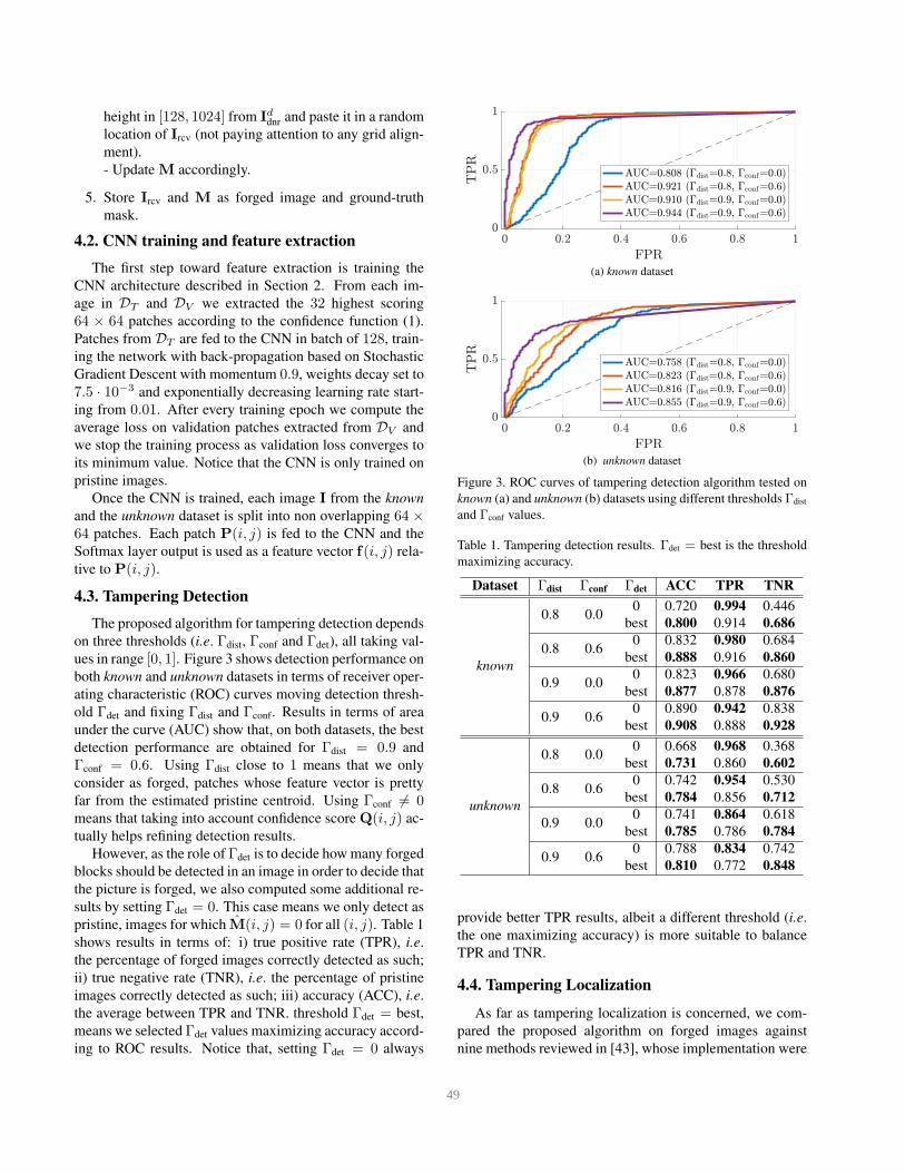
4.3. Tampering Detection

The proposed algorithm for tampering detection depends

on three thresholds (i.e. Γdist, Γconf and Γdet), all taking val-

ues in range [0, 1]. Figure 3 shows detection performance on

both known and unknown datasets in terms of receiver oper-

ating characteristic (ROC) curves moving detection thresh-

old Γdet and fixing Γdist and Γconf. Results in terms of area

under the curve (AUC) show that, on both datasets, the best

detection performance are obtained for Γdist = 0.9 and

Γconf = 0.6. Using Γdist close to 1 means that we only

consider as forged, patches whose feature vector is pretty

far from the estimated pristine centroid. Using Γconf 6= 0means that taking into account confidence score Q(i, j) ac-

tually helps refining detection results.

However, as the role of Γdet is to decide how many forged

blocks should be detected in an image in order to decide that

the picture is forged, we also computed some additional re-

sults by setting Γdet = 0. This case means we only detect as

pristine, images for which M(i, j) = 0 for all (i, j). Table 1

shows results in terms of: i) true positive rate (TPR), i.e.

the percentage of forged images correctly detected as such;

ii) true negative rate (TNR), i.e. the percentage of pristine

images correctly detected as such; iii) accuracy (ACC), i.e.

the average between TPR and TNR. threshold Γdet = best,

means we selected Γdet values maximizing accuracy accord-

ing to ROC results. Notice that, setting Γdet = 0 always

(a) known dataset

(b) unknown dataset

Figure 3. ROC curves of tampering detection algorithm tested on

known (a) and unknown (b) datasets using different thresholds Γdist

and Γconf values.

Table 1. Tampering detection results. Γdet = best is the threshold

maximizing accuracy.

Dataset Γdist Γconf Γdet ACC TPR TNR

known

0.8 0.00 0.720 0.994 0.446

best 0.800 0.914 0.686

0.8 0.60 0.832 0.980 0.684

best 0.888 0.916 0.860

0.9 0.00 0.823 0.966 0.680

best 0.877 0.878 0.876

0.9 0.60 0.890 0.942 0.838

best 0.908 0.888 0.928

unknown

0.8 0.00 0.668 0.968 0.368

best 0.731 0.860 0.602

0.8 0.60 0.742 0.954 0.530

best 0.784 0.856 0.712

0.9 0.00 0.741 0.864 0.618

best 0.785 0.786 0.784

0.9 0.60 0.788 0.834 0.742

best 0.810 0.772 0.848

provide better TPR results, albeit a different threshold (i.e.

the one maximizing accuracy) is more suitable to balance

TPR and TNR.

4.4. Tampering Localization

As far as tampering localization is concerned, we com-

pared the proposed algorithm on forged images against

nine methods reviewed in [43], whose implementation were

7 49

(a) known dataset

(b) unknown dataset

Figure 4. Accuracy and TPR on known (a) and unknown (b)

datasets using our algorithm (left hand side of dashed line) with

different thresholds (Γdist, Γconf) and state-of-the-art algorithms

(right hand side of dashed gray line). Our best accuracy and TPR

results are reported with dashed blue and orange lines.

made available in the toolbox presented in the same paper.

More specifically, we took into account all algorithms pre-

sented in Section 2, as they do not need any additional prior

information on images under analysis (e.g. PRNUs, JPEG

quantization matrix, etc.).

As evaluation metrics, we decided to rely on: i) true

positive rate (TPR), i.e. the percentage of forged pixels

correctly detected as such; ii) balanced accuracy (ACC),

i.e. the average between TPR and the percentage of cor-

rectly detected pristine pixels. However, differently from

our method, state-of-the-art considered ones output a float

tampering mask. In order to enable a fair comparison, we

binarized float masks using the threshold that maximizes

each state-of-the-art algorithm accuracy.

Figure 4 shows results obtained with our method for dif-

ferent values of thresholds Γdist and Γconf, together with

state-of-the-art methods. Notice that, our method achieves

best results when Γconf = 0. This means that for localiza-

tion purpose, it is better to discard confidence Q(i, j) infor-

mation, which instead turned to be paramount for detection

purpose. Regarding comparison against state-of-the-art, it

is possible to notice that our algorithm outperforms all con-

sidered baseline solutions. This is due to the fact that con-

sidered baselines are tailored to different kinds of tamper-

ing operations. Even more interesting, the proposed method

achieves promising results even on the unknown dataset.

This means that we are able to cope with composition forg-

eries even when used cameras do not belong to the CNN

training set. Moreover, it is possible to notice that even by

slightly varying thresholds Γdist and Γconf, our results do not

drop under baselines performance, showing a good degree

of robustness also to the choice of sub-optimal parameters.

5. Conclusions

In this paper we presented an algorithm for tampering

detection and localization to expose splicing forgeries oper-

ated using images from different camera models. The pro-

posed method exploits a CNN to extract features capturing

camera model traces from image patches. Features are clus-

tered into two groups (i.e. pristine or forged) using an iter-

ative algorithm, and information about patches locations is

further used to refine forgery localization estimation.

Evaluation carried out on a dataset of 2 000 images ob-

tained from 26 camera models shows that the proposed al-

gorithm is able to detect forged images with accuracy of

0.91 if camera models involved in forgeries have been used

during CNN training. If camera models involved in forg-

eries have never been used for training, detection accuracy

still remains as high as 0.81. Results on tampering localiza-

tion shows that it is possible to detect forged regions with

accuracy about 0.90 and 0.82 depending on the knowledge

(or not) of the used camera models at training stage. This

makes the proposed method more accurate than alternative

baseline solutions selected from [43].

Future work will follow two parallel research lines. On

one hand, we will explore the possibility of specializing the

used CNN to learn characteristics of additional processing

steps in addition to traces of camera models (e.g. resizing,

rotations, blurring, etc.). On the other hand, we will study

how to use CNN capabilities directly for localization pur-

pose by training also on forged images.

Acknowledgment

This material is based on research sponsored by DARPA

and Air Force Research Laboratory (AFRL) under agree-

ment number FA8750-16-2-0173. The U.S. Government

is authorized to reproduce and distribute reprints for Gov-

ernmental purposes notwithstanding any copyright notation

thereon. The views and conclusions contained herein are

those of the authors and should not be interpreted as nec-

essarily representing the official policies or endorsements,

either expressed or implied, of DARPA and Air Force Re-

search Laboratory (AFRL) or the U.S. Government.

8 50

References

[1] E. Ardizzone, A. Bruno, and G. Mazzola. Copy Move

Forgery Detection by Matching Triangles of Keypoints.

IEEE Transactions on Information Forensics and Security

(TIFS), 10:2084–2094, 2015.

[2] B. Bayar and M. C. Stamm. A Deep Learning Approach

To Universal Image Manipulation Detection Using A New

Convolutional Layer. In Information Hiding and Multimedia

Security, 2016.

[3] T. Bianchi and A. Piva. Detection of nonaligned double

JPEG compression based on integer periodicity maps. IEEE

Transactions on Information Forensics and Security (TIFS),

7:842–848, 2012.

[4] L. Bondi, L. Baroffio, D. Guera, P. Bestagini, E. J. Delp, and

S. Tubaro. First Steps Toward Camera Model Identification

With Convolutional Neural Networks. IEEE Signal Process-

ing Letters (SPL), 24:259–263, 2017.

[5] L. Bondi, D. Guera, L. Baroffio, P. Bestagini, E. J. Delp, and

S. Tubaro. A preliminary study on convolutional neural net-

works for camera model identification. In IS&T Electronic

Imaging (EI), 2017.

[6] G. Cao, Y. Zhao, R. Ni, L. Yu, and H. Tian. Forensic detec-

tion of median filtering in digital images. In IEEE Interna-

tional Conference on Multimedia and Expo (ICME), 2010.

[7] J. Chen, X. Kang, Y. Liu, and Z. J. Wang. Median Filtering

Forensics Based on Convolutional Neural Networks. IEEE

Signal Processing Letters (SPL), 22:1849–1853, 2015.

[8] V. Conotter, P. Comesana, and F. Perez-Gonzalez. Forensic

analysis of full-frame linearly filtered JPEG images. In IEEE

International Conference on Image Processing (ICIP), 2013.

[9] D. Cozzolino and G. Poggi. Autoencoder with recurrent neu-

ral networks for video forgery detection Autoencoder with

recurrent neural networks for video forgery detection. In

IS&T Electronic Imaging (EI), 2017.

[10] D. Cozzolino and L. Verdoliva. Single-image splicing lo-

calization through autoencoder-based anomaly detection. In

IEEE International Workshop on Information Forensics and

Security (WIFS), 2016.

[11] A. E. Dirik and N. Memon. Image tamper detection based

on demosaicing artifacts. In IEEE International Conference

on Image Processing (ICIP), 2009.

[12] H. Farid. Exposing Digital Forgeries From JPEG Ghosts.

IEEE Transactions on Information Forensics and Security

(TIFS), 4:154–160, 2009.

[13] P. Ferrara, T. Bianchi, A. De Rosa, and A. Piva. Image

forgery localization via fine-grained analysis of CFA arti-

facts. IEEE Transactions on Information Forensics and Se-

curity (TIFS), 7:1566–1577, 2012.

[14] M. Fontani, S. Member, T. Bianchi, and A. D. Rosa. A

Framework for Decision Fusion in Image Forensics Based

on Dempster Shafer Theory of Evidence. IEEE Transac-

tions on Information Forensics and Security (TIFS), 8:593–

607, 2013.

[15] L. Gaborini, P. Bestagini, S. Milani, M. Tagliasacchi, and

S. Tubaro. Multi-clue image tampering localization. In IEEE

International Workshop on Information Forensics and Secu-

rity (WIFS), 2015.

[16] T. Gloe and R. Bohme. The Dresden Image Database for

Benchmarking Digital Image Forensics. Journal of Digital

Forensic Practice, 3:150–159, 2010.

[17] M. Goljan and J. Fridrich. Camera identification from

cropped and scaled images. In SPIE Electronic Imaging (EI),

2008.

[18] J. Hosang, M. Omran, R. Benenson, and B. Schiele. Taking a

deeper look at pedestrians. In IEEE Conference on Computer

Vision and Pattern Recognition (CVPR), 2015.

[19] M. Kirchner. Fast and reliable resampling detection by spec-

tral analysis of fixed linear predictor residue. In ACM work-

shop on Multimedia and Security (MM&Sec), 2008.

[20] M. Kirchner and J. Fridrich. On detection of median filtering

in digital images. In SPIE Media Forensics and Security,

2010.

[21] M. Kirchner and T. Gloe. Forensic Camera Model Identifica-

tion. In Handbook of Digital Forensics of Multimedia Data

and Devices. John Wiley & Sons, Ltd, 2015.

[22] N. Krawetz. A Picture’s Worth... Hacker Factor Solutions,

pages 1–31, 2007.

[23] A. Krizhevsky, I. Sulskever, and G. E. Hinton. ImageNet

Classification with Deep Convolutional Neural Networks.

Advances in Neural Information and Processing Systems

(NIPS), pages 1–9, 2012.

[24] Y. LeCun, L. Bottou, Y. Bengio, and P. Haffner. Gradient-

based learning applied to document recognition. Proceed-

ings of the IEEE, 86:2278–2323, 1998.

[25] W. Li, Y. Yuan, and N. Yu. Passive detection of doctored

JPEG image via block artifact grid extraction. Signal Pro-

cessing, 89:1821–1829, 2009.

[26] M. Lin, Q. Chen, and S. Yan. Network In Network. arXiv

preprint, page 10, 2013.

[27] Z. Lin, J. He, X. Tang, and C. K. Tang. Fast, automatic and

fine-grained tampered JPEG image detection via DCT coef-

ficient analysis. Pattern Recognition, 42:2492–2501, 2009.

[28] J. Lukas, J. Fridrich, and M. Goljan. Determining digital

image origin using sensor imperfections. In Proceedings of

the SPIE, 2005.

[29] J. Lukas, J. Fridrich, and M. Goljan. Digital Camera Identifi-

cation From Sensor Pattern Noise. IEEE Transactions on In-

formation Forensics and Security (TIFS), 1:205–214, 2006.

[30] B. Mahdian and S. Saic. Using noise inconsistencies

for blind image forensics. Image and Vision Computing,

27:1497–1503, 2009.

[31] A. Piva. An overview on image forensics. ISRN Signal Pro-

cessing, 2013:22, 2013.

[32] A. Popescu and H. Farid. Exposing digital forgeries by de-

tecting traces of resampling. IEEE Transactions on Signal

Processing (TSP), 53:758–767, 2005.

[33] Y. Qian, J. Dong, W. Wang, and T. Tan. Deep learning for

steganalysis via convolutional neural networks. In SPIE Me-

dia Watermarking, Security, and Forensics, 2015.

[34] A. Rocha, W. Scheirer, T. Boult, and S. Goldenstein. Vision

of the unseen: Current trends and challenges in digital im-

age and video forensics. ACM Computing Surveys, 43:1–42,

2011.

9 51

[35] M. C. Stamm, Min Wu, and K. J. R. Liu. Information Foren-

sics: An Overview of the First Decade. IEEE Access, 1:167–

200, 2013.

[36] C. Szegedy, W. Liu, Y. Jia, and P. Sermanet. Going deeper

with convolutions. In IEEE Conference on Computer Vision

and Pattern Recognition (CVPR), 2015.

[37] Y. Taigman, M. Yang, M. Ranzato, and L. Wolf. DeepFace:

Closing the Gap to Human-Level Performance in Face Verifi-

cation. In IEEE Conference on Computer Vision and Pattern

Recognition (CVPR), 2014.

[38] T. H. Thai, R. Cogranne, F. Retraint, and T.-N.-C. Doan.

JPEG Quantization Step Estimation and Its Applications to

Digital Image Forensics. IEEE Transactions on Information

Forensics and Security (TIFS), 12:123–133, 2017.

[39] D. Tome, F. Monti, L. Baroffio, L. Bondi, M. Tagliasacchi,

and S. Tubaro. Deep Convolutional Neural Networks for

pedestrian detection. Signal Processing: Image Communi-

cation, 47:482–489, 2016.

[40] A. Tuama, F. Comby, and M. Chaumont. Camera model

identification with the use of deep convolutional neural net-

works. In IEEE International Workshop on Information

Forensics and Security (WIFS), 2016.

[41] L. Verdoliva, D. Cozzolino, and G. Poggi. A feature-based

approach for image tampering detection and localization. In

IEEE International Workshop on Information Forensics and

Security (WIFS), 2014.

[42] S. Ye, Q. Sun, and E.-C. Chang. Detecting Digital Image

Forgeries by Measuring Inconsistencies of Blocking Artifact.

In IEEE International Conference on Multimedia and Expo

(ICME), volume 117543, 2007.

[43] M. Zampoglou, S. Papadopoulos, and Y. Kompatsiaris.

Large-scale evaluation of splicing localization algorithms

for web images. Multimedia Tools and Applications,

76(4):4801–4834, feb 2017.

1052