Forecasting Sales of Slow and Fast Moving Inventories04 Sales of Slow and Fast Moving Inventories...
30
ISSN 1440-771X ISBN 0 7326 1062 1 M O N A S H U N I V E R S I T Y AUSTRALIA Forecasting Sales of Slow and Fast Moving Inventories Ralph Snyder Working Paper 7/99 June 1999 DEPARTMENT OF ECONOMETRICS AND BUSINESS STATISTICS
Transcript of Forecasting Sales of Slow and Fast Moving Inventories04 Sales of Slow and Fast Moving Inventories...
ISSN 1440-771X
ISBN 0 7326 1062 1
M O N A S H U N I V E R S I T Y
AUSTRALIA
Forecasting Sales of Slow and Fast Moving Inventories
Ralph Snyder
Working Paper 7/99
June 1999
DEPARTMENT OF ECONOMETRICS
AND BUSINESS STATISTICS

C:\data\research\nonneg\Forecasting Sales of Slow and Fast Moving Inventories04
06/07/2001
Forecasting Sales of Slow and Fast Moving Inventories
Ralph Snyder
Department of Econometrics and Business Statistics
Monash University
Page proofs should be sent to:
Associate Professor R. D. Snyder
PO Box 11E
Department of Econometrics and Business Statistics
Monash University
Australia 3800
Corresponding author:
Telephone: + 613 9905 2366
Fax: 613 9905 5474
Email: [email protected]
2/29
Forecasting Sales of Slow and Fast Moving Inventories
Keywords
demand forecasting, inventory control, simulation, parametric bootstrapping, time series
analysis.
Abstract
Traditional computerised inventory control systems usually rely on exponential smoothing to
forecast the demand for fast moving inventories. Practices in relation to slow moving
inventories are more varied, but the Croston method is often used. It is an adaptation of
exponential smoothing that 1) incorporates a Bernoulli process to capture the sporadic nature of
demand and 2) allows the average variability to change over time. The Croston approach is
critically appraised in this paper. Corrections are made to underlying theory and modifications
are proposed to overcome certain implementation difficulties. A parametric bootstrap approach
is outlined that integrates demand forecasting with inventory control. The approach is illustrated
on real demand data for car parts.

3/29
1. Introduction
An understanding of key features of demand data is important when developing computer
systems for forecasting and inventory control. Plots of demand for three parts carried by an
Australian subsidiary of a Japanese car company are shown in Figure 1. It is emphasised that the
data genuinely measure demand and not sales. The data are of Australia-wide monthly demand
over a three-year period. The raw data may be found in Appendix 2. It should be emphasised
the series are not meant to be representative of all types of demand series encountered in
practice. The series were chosen because they were considered to be typical of those that cause
difficulties in conventional inventory control systems.
-------------------------------------------------------------------------------------------------------------------
Insert Figure 1 about here
--------------------------------------------------------------------------------------------------------------------
Car Part 1 is slow moving and unaffected by structural change. Car Part 2 is also slow moving,
but its level and variability appear to be in decline: it is possibly reaching the end of its life
cycle. Car Part 3 is relatively fast moving, but is also in a declining phase. The graphs for parts
1 and 2 highlight the important point that demand series can contain many zero values.
Although not illustrated here, series with a majority of zero values are common. A forecasting
technique that allows for the possibility of zero values, but still works with fast moving
inventories like Car Part 3, is most desirable. It eliminates the need to make artificial
distinctions between slow and fast moving items, something that researchers (Johnston and
Boylan, 1996b) have perceived as being a critical issue in applied forecasting.
Simple exponential smoothing (Brown,1959) has been the mainstay of forecasting for inventory
control (Gardner, 1985). A special adaptation (Croston, 1972) of this method, incorporating a
Bernoulli process, is often recommended for cases with intermittent demand (Willemain et al,
1994). The focus of this paper is on an improved version of the Croston approach and its use in
inventory control. Emphasis is placed on the need to correctly specify the statistical models for
the generation of approximations to the probability distributions of lead-time demand. A
parametric bootstrap method is proposed for determining appropriate values for inventory
control parameters. The proposed approach and its more traditional counterparts are applied to
the demand data in Figure 1. They are compared using computed values of ordering parameters
required for inventory control.
4/29
2. Current Approaches to Forecasting
2.1 Simple Exponential Smoothing (SES)
A local level model, a special case of the single source of error state-space family of models
(Snyder, 1985; Ord, Koehler and Snyder, 1997), is used as the statistical framework for simple
exponential. It is a structural representation of the ARIMA(0,1,1) process, the latter being the
framework traditionally used for simple exponential smoothing (Muth, 1960; Box and Jenkins,
1976). In the local level model, demand ty during a typical period t, is determined by the
equation
1t t ty µ ε−= + . (2.1)
The first term on the right hand side of this equation is referred to as the underlying level. It is
lagged because the demands that flow in during period t are assumed to depend on the state of
the market at the start of period t. The second term is a disturbance that represents unanticipated
demand. All disturbances are normally distributed with mean 0 and common variance 2σ . It is
also assumed that tε is uncorrelated with all earlier underlying levels.
The underlying level potentially changes over time in response to unanticipated changes in
market structure. It is governed by the transition equation
1t t tµ µ αε−= + (2.2)
where the so-called smoothing parameter α determines the rate of change in the underlying
level. It is possible that 0α = : the case of no structural change. The transition equation is
seeded with
0µ µ= . (2.3)
The seed level µ , the smoothing parameter α and the variance 2σ are unknown and must be
estimated from a sample 1 2, , , ny y yK of size n. For any trial values of these quantities, simple
exponential smoothing may be applied to determine a series of one-step ahead prediction errors
1 2, , , ne e eK . Simple exponential smoothing involves 1| , , , ,t t tm y yµ µ α= K , a quantity that
will be referred to as the local level. This notation reflects the fact that the local level, at any
point of time, depends on the past trajectory of the time series, together with the specified
values of the seed level µ and smoothing parameter α . At stage t the algorithm entails the
calculation of the one-step ahead prediction error
t t te y m= − (2.4)
and the revision of the local level with the recurrence relationship

5/29
1t t tm m eα−= + . (2.5)
In contrast to the original unconditional tµ , the mt are fixed quantities for specified values of
µ and α .
In practice, the seed level µ is often estimated using a heuristic such as the simple average of
the first three series values. An alternative is to find that value that minimises the sum of
squared errors 2
1
n
tt
e=
∑ . There are cogent arguments for both strategies and it is not a purpose of
this paper to dwell on the choice between them. In this paper, the optimisation approach is
adopted. One advantage is that exponential smoothing then accommodates the important special
case of no structural change (where 0α = ). It collapses to a classical simple average in this
circumstance. If there is a preference in practice for the heuristic, the method presented here can
be adapted accordingly. Forecasts are insensitive to the seed value when α is not close to zero,
so both initialisation strategies yield similar results in this circumstance. The least squares
estimates are designated by µ̂ and $α . Estimates of the corresponding conditional means are
denoted by $mt . The estimate of the variance of unanticipated demand is given by the formula
2 2
1
ˆn
tt
e nσ=
= ∑ (2.6)
Prediction with simple exponential smoothing has traditionally been handled using ad-hoc
model-free strategies. More reliable analytical approaches for deriving the distributions of lead-
time demand (Johnston and Harrison, 1986; Harvey and Snyder, 1990; Snyder, Koehler and
Ord, 1999) now exist and may be used in their place. A simple alternative, that exploits the
extensive computational capacities of modern computers, is based on the following simulation
method. Assuming that the problem is to find the distribution of aggregate demand over a lead-
time n n h+ +1,� �, it consists of the following steps:
1. Use Monte Carlo random number generation methods to obtain values for the errors
1, ,n n hε ε+ +K from a normal distribution with mean zero and variance 2σ .
2. Use the local level model, as described by equations (2.1) and (2.2), to generate a
realisation y yn n h+ +1, ,K of future series values.
3. Calculate lead-time demand 1
n h
tt n
y+
= +∑ .
This procedure is repeated many times. Replication i of lead-time demand is denoted by
6/29
( )
1
n hi
tt n
y+
= +∑ . Taken together, these quantities form a sample that may be used to approximate the
lead-time demand distribution.
Steps 1 and 2 of this simulation procedure requires values for µ , α and σ 2 , but these are
unknown. The corresponding least squares estimates are used in their place, meaning that the
simulation method becomes what is commonly called a ‘parametric bootstrap’. Like all such
approaches, the effect of sampling error is ignored. The consequent loss of accuracy is usually
tolerable because sampling error is a second-order effect. Despite this drawback, the parametric
bootstrap method provides a much sounder basis for the determination of the lead-time demand
distribution than the ad hoc approaches commonly in use.
2.2 The Croston Method
It was argued by Croston (1972) that simple exponential smoothing is not appropriate for
inventories with intermittent demand. In appendix B of his paper, he outlines a model of
intermittent demand, a method for estimating key quantities in the model and a method for
predicting lead time demand for reorder level determination from a sample. The model is cast as
an ARIMA(0,1,1) process that is assumed to apply only at those intermittent periods when
transactions occur. A Bernoulli process governs the time between such active periods, the
discrete analogue of a Poisson process.
The Croston model may be seen as an adaptation of the conventional local level model to allow
for the intermittent nature of demand. An additional random variable tx is used to indicate
those periods in which transactions take place. This binary random variable is governed by a
Bernoulli distribution with parameter p, the probability of there being some demand in a given
period. It is used to force the local level and disturbance variance to zero in inactive periods.
The model is
1t t t ty x µ ε−= + (2.7)
where
1t t tµ µ αε−= + (2.8)
The disturbances are still independently and normally distributed, with a common mean 0.
However, the variance in period t is augmented by the binary variable to become 2tx σ . The
ARIMA model in the original representation has been replaced by its state space analogue, the
local level model. This is a change of form, rather than substance, to clarify the link with
exponential smoothing. Note that, unlike the underlying level tµ , both p and 2σ are not
7/29
subscripted by time. These quantities are implicitly assumed to remain unchanged over time.
The Croston method, as distinct from his model, involves finding exponentially weighted
moving averages (EWMA) of three quantities:
1. the positive series values yt ,
2. the associated absolute errors te ,
3. the elapsed times between successive active periods (periods in which transactions
occur).
It then involves finding the underlying mean demand from the ratio of the first and third
EWMA’s.
The EWMA’s in his method use the same smoothing parameter. Croston is vague about how
this quantity should be chosen. He indicates “if the series i s short it may have to be chosen
arbitrarily from experience”. He is also vague about the choice of seed values for the EWMA’s.
He seems to place himself in the heuristic rather than the optimisation school. As indicated
earlier, this is a legitimate stance to take when confronted with the realities of business
environment.
The exponentially weighted averages in steps 2 and 3 of his method are designed to detect and
allow for changes in the variability of demand and mean frequency of active periods. A method
along these lines would therefore be expected to work well for Car Part 2 depicted in Figure 1.
Because of its focus on intermittent demands, the Croston method has been the subject of
considerable interest. Nevertheless, a number of problems have been identified. Rao (1973)
found errors in the algebra. Johnston and Boylan (1996a) expressed concern about a measure of
the variability of demand that does not incorporate the effect of uncertainty in the elapsed times
between active periods. Their proposed solution based on renewal theory, however, assumes
that means and variances are constant, something that diverges from the spirit of the exponential
smoothing methods. It is not suitable, for example, for inventories like Car Part 2 depicted in
Figure 1. Thus, it can be argued that the variability problem they identified with the Croston
method remains to be resolved.
There are further problems with Croston’s paper that have not so far been identified in print.
Inconsistencies exist between model and method in relation to the second and third
exponentially weighted averages. In order to justify the use of these EWMA’s, it is necessary to
assume that σ 2 and p change over time. It may be true in practice that these quantities change.

8/29
But they are assumed to be constant in his model. For consistency it is necessary to replace the
offending EWMA’s by the formulae 2 2
1 1
ˆn n
t tt t
e xσ= =
= ∑ ∑ and 1
ˆn
tt
p x n=
= ∑ . This modified
version of his method will be called MCROST.
3. New Methods
The simulation method outlined for simple exponential smoothing may be adapted to generate
an approximation for the lead-time demand distribution from the Croston model. An iteration
would involve the following steps:
1. Generate values for the errors 1, ,n n hε ε+ +K from a normal distribution with mean 0 and
variance 2σ .
2. Generate values for the indicator variables x xn n h+ +1, ,K from a Bernoulli distribution
with probability p.
3. Generate a realisation y yn n h+ +1, ,K of future series values from the modified local level
model equations (2.7) and (2.8).
4. Calculate lead-time demand with ytt n
n h
= +
+
∑1
.
There is, however, a serious logical difficulty. Nothing in the local level component of the
Croston model inhibits the simulation of negative synthetic data, something that is incompatible
with the reality that demand can never be negative. One possible way around this difficulty is to
apply exponential smoothing to the logarithm of the data. The weakness of this strategy is that
the raw series may contain zeroes. ( )log 0 does not exist!
Another possible fix might be to round all negative values to zero. There would then be two
sources of zeros in the model: the Bernoulli process and the local level model. It would not be
possible to distinguish between both sources in real data. The Croston model is not viable as a
mechanism for generating prediction distributions without an alteration to overcome this basic
flaw.
3.1 Log-Space Adaptation (LOG)
An adaptation that leads to a new model, and hence a new approach to forecasting, is to enforce
non-negative demands using the equation
( )expt t ty x y+ = . (3.1)
9/29
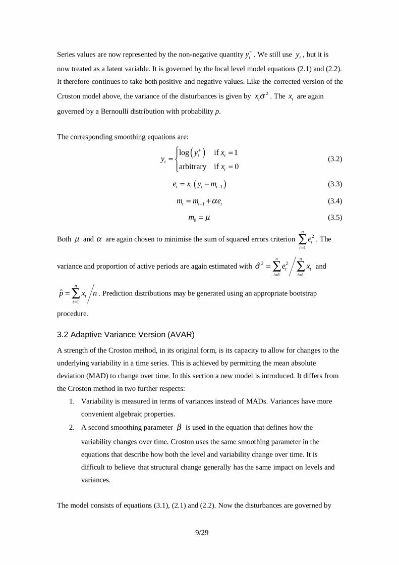
Series values are now represented by the non-negative quantity yt+ . We still use yt , but it is
now treated as a latent variable. It is governed by the local level model equations (2.1) and (2.2).
It therefore continues to take both positive and negative values. Like the corrected version of the
Croston model above, the variance of the disturbances is given by 2tx σ . The tx are again
governed by a Bernoulli distribution with probability p.
The corresponding smoothing equations are:
( )log if 1
arbitrary if 0
t tt
t
y xy
x
+ == =
(3.2)
( )1t t t te x y m −= − (3.3)
1t t tm m eα−= + (3.4)
0m µ= (3.5)
Both µ and α are again chosen to minimise the sum of squared errors criterion 2
1
n
tt
e=
∑ . The
variance and proportion of active periods are again estimated with 2 2
1 1
ˆn n
t tt t
e xσ= =
= ∑ ∑ and
1
ˆn
tt
p x n=
= ∑ . Prediction distributions may be generated using an appropriate bootstrap
procedure.
3.2 Adaptive Variance Version (AVAR)
A strength of the Croston method, in its original form, is its capacity to allow for changes to the
underlying variability in a time series. This is achieved by permitting the mean absolute
deviation (MAD) to change over time. In this section a new model is introduced. It differs from
the Croston method in two further respects:
1. Variability is measured in terms of variances instead of MADs. Variances have more
convenient algebraic properties.
2. A second smoothing parameter β is used in the equation that defines how the
variability changes over time. Croston uses the same smoothing parameter in the
equations that describe how both the level and variability change over time. It is
difficult to believe that structural change generally has the same impact on levels and
variances.
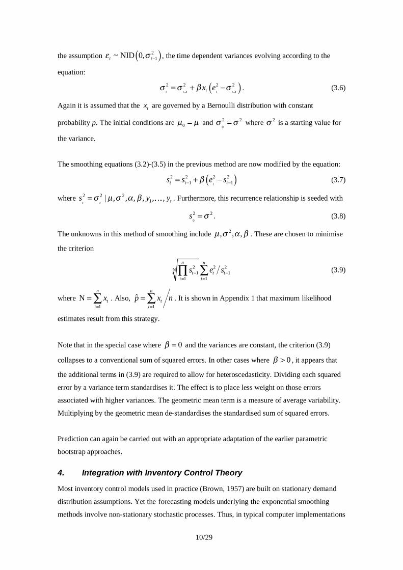
The model consists of equations (3.1), (2.1) and (2.2). Now the disturbances are governed by
10/29
the assumption ( )21~ NID 0,t tε σ − , the time dependent variances evolving according to the
equation:
( )1 1
2 2 2 2
t t t ttx eσ σ β σ− −
= + − . (3.6)
Again it is assumed that the tx are governed by a Bernoulli distribution with constant
probability p. The initial conditions are 0µ µ= and 0
2 2σ σ= where 2σ is a starting value for
the variance.
The smoothing equations (3.2)-(3.5) in the previous method are now modified by the equation:
( )2 2 2 21 1tt t ts s e sβ− −= + − (3.7)
where 2 2 21| , , , , , ,
t t ts y yσ µ σ α β= K . Furthermore, this recurrence relationship is seeded with
0
2 2s σ= . (3.8)
The unknowns in this method of smoothing include 2, , ,µ σ α β . These are chosen to minimise
the criterion
2 2 2N
1 111
n n
t t ttt
s e s− −==∑∏ (3.9)
where 1
Nn
tt
x=
= ∑ . Also, 1
ˆn
tt
p x n=
= ∑ . It is shown in Appendix 1 that maximum likelihood
estimates result from this strategy.
Note that in the special case where 0β = and the variances are constant, the criterion (3.9)
collapses to a conventional sum of squared errors. In other cases where 0β > , it appears that
the additional terms in (3.9) are required to allow for heteroscedasticity. Dividing each squared
error by a variance term standardises it. The effect is to place less weight on those errors
associated with higher variances. The geometric mean term is a measure of average variability.
Multiplying by the geometric mean de-standardises the standardised sum of squared errors.
Prediction can again be carried out with an appropriate adaptation of the earlier parametric
bootstrap approaches.
4. Integration with Inventory Control Theory
Most inventory control models used in practice (Brown, 1957) are built on stationary demand
distribution assumptions. Yet the forecasting models underlying the exponential smoothing
methods involve non-stationary stochastic processes. Thus, in typical computer implementations

11/29
of the theory, forecasts from non-stationary models are fed into inventory formulae based on
stationary demand distribution assumptions. The use of inconsistent models like this is dictated
by the fact that the theory of non-stationary inventory control is inherently more complex than
its stationary counterpart and is therefore perceived, rightly or wrongly, as more difficult to
implement in practice (Hax and Candea, 1984, pp 239-240).
Satisfactory methods for inventory control, based on the same assumptions as exponential
smoothing, are yet to be devised. It is not intended to propose a solution here to this difficult
problem. We shall instead follow current practice and show how to adapt the traditional
approach to inventory control to the case where a lead-time demand distribution has been
approximated by a simulated sample. Thus the working hypothesis is that the structure of the
demand process remains unchanged in all future periods, even though we have allowed for
structural change in the past while generating the required forecasts. Use of a hypothesis like
this is not ideal, but it is necessary until a workable non-stationary inventory theory has been
developed.
Brown’s approach to inventory control was adapted in Snyder (1984) to handle demands
generated by gamma probability distribution. The methods described here are similar except the
gamma distribution is replaced by the simulated demand data from the above forecasting
procedures.
4.1 Order-Up-To Level System: Zero Lead Time Case
When there is no delivery lag, and hence no need to account for outstanding replenishment
orders, the order-up-to level (OUL) represents the ideal level for stock. Assuming that
replenishment orders are only placed periodically, the aim is to order enough to ensure that
stock rises to this ideal level. At the beginning of each period the order-up-to level then
represents the amount of stock available to meet an uncertain demand during the following
review period. Shortages occur if demand during a review period exceeds the OUL. Thus the
choice of the OUL is critical to the successful operation of the system. The distinctive feature of
the customer service level approach is that a performance target is set in terms of what may be
termed the fill-rate. This is the proportion of demand, on average, that is satisfied without
backlogging. The aim is choose the OUL so that the fill-rate equals a level specified by
management (eg 95 percent).
Let y yn nN
+ +11
1b g b g, ,K denote the simulated demands for the next period. If S represents the
unknown OUL, the fill-rate statistic may be defined as an ‘ensemble’ average
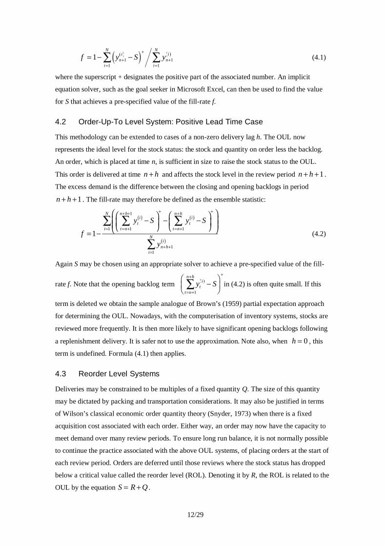
12/29
f y S yni
i
N
ni
i
N
= − −+
+
=+
=∑ ∑1 1
11
1
b g b g� � (4.1)
where the superscript + designates the positive part of the associated number. An implicit
equation solver, such as the goal seeker in Microsoft Excel, can then be used to find the value
for S that achieves a pre-specified value of the fill-rate f.
4.2 Order-Up-To Level System: Positive Lead Time Case
This methodology can be extended to cases of a non-zero delivery lag h. The OUL now
represents the ideal level for the stock status: the stock and quantity on order less the backlog.
An order, which is placed at time n, is sufficient in size to raise the stock status to the OUL.
This order is delivered at time n h+ and affects the stock level in the review period n h+ +1 .
The excess demand is the difference between the closing and opening backlogs in period
n h+ +1 . The fill-rate may therefore be defined as the ensemble statistic:
( ) ( )
( )
1
1 1 1
11
1
N n h n hi i
t ti t n t n
Ni
n hi
y S y S
fy
+ ++ + +
= = + = +
+ +=
− − − = −∑ ∑ ∑
∑ (4.2)
Again S may be chosen using an appropriate solver to achieve a pre-specified value of the fill-
rate f. Note that the opening backlog term y Sti
t n
n ha f −
���
���= +
+ +
∑1
in (4.2) is often quite small. If this
term is deleted we obtain the sample analogue of Brown’s (1959) partial expectation approach
for determining the OUL. Nowadays, with the computerisation of inventory systems, stocks are
reviewed more frequently. It is then more likely to have significant opening backlogs following
a replenishment delivery. It is safer not to use the approximation. Note also, when h = 0 , this
term is undefined. Formula (4.1) then applies.
4.3 Reorder Level Systems
Deliveries may be constrained to be multiples of a fixed quantity Q. The size of this quantity
may be dictated by packing and transportation considerations. It may also be justified in terms
of Wilson’s classical economic order quantity theory (Snyder, 1973) when there is a fixed
acquisition cost associated with each order. Either way, an order may now have the capacity to
meet demand over many review periods. To ensure long run balance, it is not normally possible
to continue the practice associated with the above OUL systems, of placing orders at the start of
each review period. Orders are deferred until those reviews where the stock status has dropped
below a critical value called the reorder level (ROL). Denoting it by R, the ROL is related to the
OUL by the equation S R Q= + .
13/29
Matters are made more complicated in this type of system by the fact that the stock status
following each review is no longer constant. It is shown in Hadley and Whitin (1963), that if the
demand distribution is stationary, the stock status immediately following each review can be
modelled as a doubly stochastic Markov Chain. From this they establish that its movements are
ultimately governed by a uniform steady state distribution. The mass of this distribution is 1 Q
over the domain R S,� �.
To simulate the average performance of the system, N values u uN1, ,K are generated from a
uniform distribution over the unit interval 0 1,� � . Corresponding values of the stock status are
then given by R u Qi+ , so that the fill-rate is now given by
f
y R u Q y R u Q
y
ti
t
n h
i ti
it n
n h
i
N
n hi
i
N= −
− −���
��� − − −���
���
���
���=
+ + +
= +
+ +
=
+ +=
∑ ∑∑
∑1
1
1
11
11
b g b g
b g
. (4.3)
Assuming that Q is known and that management has specified a target value for the fill-rate f,
an implicit function solver can be used to find the corresponding value of the reorder level R.
This formula for the fill-rate is strictly only applicable when a stationary stochastic process
generates demands. Because it relies on the steady state distribution of the stock status, (4.3) is a
measure of the long-term performance of the system. When the non-stationary process
underlying exponential smoothing generates demands, a steady state does not exist. Given that
there is no reasonable alternative in this situation, however, the use of this formula is
recommended until the matter is properly resolved.
5. Examples
The forecasting methods and their performance are illustrated here by applying them to the
demand data in Appendix 2. This is the data depicted in Figure 1. As the Australian stores of the
company are replenished by deliveries from Japan, the delivery lead-time is assumed to be 3-
months. The review period is assumed to be one month in length because the demand data is
collated on a monthly basis. In reality, the review period is much less than this. However,
demand data collated over the shorter review period was unavailable. It is also assumed that an
OUL system is employed to control stocks. In reality, a reorder level control system is used.
This deviation from reality is adopted to ensure that differences in extraneous factors, such as
the size of Q, do not confound the conclusions.
The sample size being 36, the start of month 37 corresponds to the ‘current’ review. Any order
placed at this point of time is assumed to arrive three months later at the beginning of month 40.
14/29
The primary aim at the start of month 37, therefore, is to control inventories in month 40. A
target fill-rate of 95 percent is employed.
Five methods are compared:
GAM The gamma probability distribution approach (Snyder, 1984) for obtaining
order-up-to levels. Being based on a stationary demand process, the
associated mean and variance are estimated by a simple average and the
classical variance formula. This case is included for benchmarking
purposes.
SES This applies simple exponential smoothing, as described in section 2.1, to
the data. It ignores the possibility that the data may pertain to a slow
moving inventory.
MCROST The Croston method implemented with the modifications specified in
section 2.2.
LOG The adaptation of MCROST described in section 3.1. A log-transform is
applied to non-zero demands.
AVAR The adaptive variance approach detailed in section 3.2. The adaptive
variance recurrence relationship (3.7) is seeded with a value obtained from
the classical sample variance formula applied to the first 12-months of
data. The method proved to be unstable for optimised values of the seed
variance.
Lead-time demand distributions, for methods 2-4, are derived using suitably adapted parametric
bootstrap procedures. These are based on 10,000 replications.
Each of Tables 1-3 summarises the results for a car part. Each column corresponds to one of
above methods. It is important to note that some of the results in the final two columns are not
comparable with those in earlier columns because they refer to statistics calculated in log-space
rather than raw-space. The final row contains the most important results: the OULs that achieve
the 95 percent fill-rate target. These OULs are all expressed in terms of the raw-space and are
therefore comparable. The performance of a method can be gauged by the size of the associated
OUL. Ideally, the OUL should be as low as possible. The rows before the last one contain
auxiliary information. The first row provides the simple average of the entire series. Rows 2 and
3 contain levels for the start and end of the sampling period. The next two rows list the
estimates of the level and variance equation smoothing parameters. The three subsequent rows
contain variance estimates. The next row has the estimate of the active periods proportion. The
second last row is provided for those methods that do not impose non-negativity conditions on
demands.
15/29
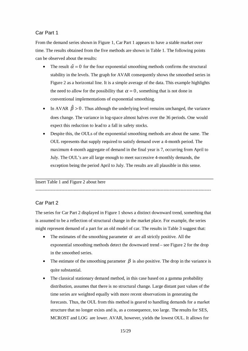
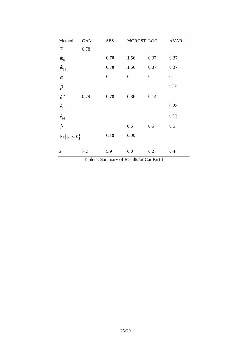
Car Part 1
From the demand series shown in Figure 1, Car Part 1 appears to have a stable market over
time. The results obtained from the five methods are shown in Table 1. The following points
can be observed about the results:
• The result ˆ 0α = for the four exponential smoothing methods confirms the structural
stability in the levels. The graph for AVAR consequently shows the smoothed series in
Figure 2 as a horizontal line. It is a simple average of the data. This example highlights
the need to allow for the possibility that 0α = , something that is not done in
conventional implementations of exponential smoothing.
• In AVAR ˆ 0β > . Thus although the underlying level remains unchanged, the variance
does change. The variance in log-space almost halves over the 36 periods. One would
expect this reduction to lead to a fall in safety stocks.
• Despite this, the OULs of the exponential smoothing methods are about the same. The
OUL represents that supply required to satisfy demand over a 4-month period. The
maximum 4-month aggregate of demand in the final year is 7, occurring from April to
July. The OUL’s are all large enough to meet successive 4-monthly demands, the
exception being the period April to July. The results are all plausible in this sense.
Insert Table 1 and Figure 2 about here
-------------------------------------------------------------------------------------------------------------------
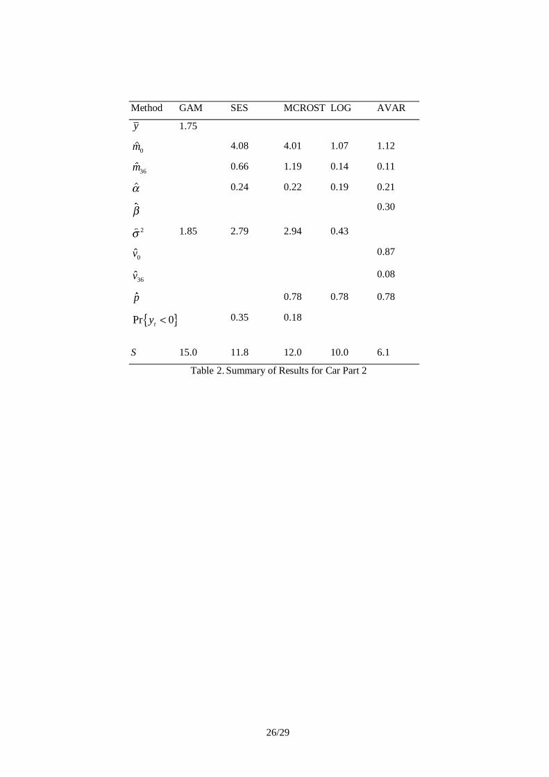
Car Part 2
The series for Car Part 2 displayed in Figure 1 shows a distinct downward trend, something that
is assumed to be a reflection of structural change in the market place. For example, the series
might represent demand of a part for an old model of car. The results in Table 3 suggest that:
• The estimates of the smoothing parameter α are all strictly positive. All the
exponential smoothing methods detect the downward trend – see Figure 2 for the drop
in the smoothed series.
• The estimate of the smoothing parameter β is also positive. The drop in the variance is
quite substantial.
• The classical stationary demand method, in this case based on a gamma probability
distribution, assumes that there is no structural change. Large distant past values of the
time series are weighted equally with more recent observations in generating the
forecasts. Thus, the OUL from this method is geared to handling demands for a market
structure that no longer exists and is, as a consequence, too large. The results for SES,
MCROST and LOG are lower. AVAR, however, yields the lowest OUL. It allows for

16/29
the decline in variability in the data. The largest 4-month run of demand in the final
year is only 4. Practitioners would probably argue that all OUL’s are too high. The
result from the AVAR method might just be acceptable.
• The proportion of 0.35 negative simulated demands for the conventional local level
model is quite high. Yet, the effect of the negative values on the OUL appears to have
been minimal.
Insert Table 2 about here
-------------------------------------------------------------------------------------------------------------------
Car Part 3
The final series consists of demand for the fast moving Car Part 3. Again, a slowly declining
market is assumed to reflect the effect of structural change. It is interesting to note that:
• The maximum 4-monthly run of demand in the final year is 167. Remarkably, AVAR
yields an OUL slightly above this figure.
• The estimate of the smoothing parameter α is about 0.2 for all exponential smoothing
methods. This indicates that structural change impacts the data. A comparison of the
OUL’s from the Gamma distribution and exponential smoothing approaches
demonstrates sizeable benefits from the use of exponentially weighted averages instead
of a simple average.
• The estimate of the smoothing parameter β is zero. The variability in the demand
series appears not to change much over time.
• The estimate of the binomial probability p is one. In this circumstance, LOG has
appropriately collapsed to classical simple exponential smoothing, albeit in log-space.
AVAR has collapsed to a variant of simple exponential smoothing that allows for
changes to variability as well as changes to the mean. In other words, these methods
provide a unified approach to forecasting demand for slow and fast moving inventories.
The distinction between slow and fast-moving inventories is made automatically
through the estimation of p. There is no need to implement separate methods of
forecasting for slow and fast moving items and to employ heuristics to distinguish
between the two cases.
• It might be expected that LOG and AVAR should yield almost identical results in this
situation. Yet, the OUL is lower for AVAR. The standard deviations for LOG is 0.14.
The estimate of the standard deviation in period 36 for AVAR is 0.08. The difference in
these figures leads to the observed difference in the associated OUL’s. Why does such a
discrepancy occur? The variances (equally weighted versions in log space) for years 1
17/29
to 3 are 0.08, 0.14 and 0.13 respectively. Thus, there was a significant increase in
relative variability between years 1 and 2. Then it stabilised between years 2 and 3.
Thus, the variance recurrence relationship is initiated with the lower value 0.08.
Because the variability stabilised in years 2 and 3, the best estimate of the smoothing
parameter β was found to be almost zero. Therefore, the variance did not adjust much
to the higher variability in the second and third years. It is not possible, on the basis of
this particular data set, to conclude that AVAR is inherently better than LOG. It might
be more satisfactory if the seed value of the variance recurrence relationship could be
optimised instead of being chosen by a heuristic. As indicated previously, however, its
optimisation with the criterion (3.9) and similar criteria seems to be unstable.
• This example highlights the need to use distinct smoothing parameters in the updating
equations for the level and variance.
Insert Table 3 about here
-------------------------------------------------------------------------------------------------------------------
6. Conclusions and Final Comments
Methods of forecasting that can be applied to both fast and slow moving inventories have been
proposed in this paper. Many features of these methods reflect the influence of Croston’s
approach to forecasting. But there are key differences, these being:
• smoothing in log-space to avoid negative demands;
• different smoothing parameters for the level and variance;
• the use of compatible models and methods;
• the use of models in a parametric bootstrap approach to generate lead-time demands;
• reorder level and order-up-to level determination using the fill-rate criterion from
bootstrapped demands;
• a constant probability in the Bernoulli process governing the occurrence of active
months.
This last point may seem to be a backward step. However, when random walk models of this
probability were implemented, maximum likelihood estimates of the smoothing parameter
associated with the resulting exponentially weighted average always turned out to be zero. It is
not clear why this should be so. One conjecture is that very large samples are required to ensure
a large enough number of inter-transaction times with which to work. In practice, such samples
are rarely available.
A feature of the methods is that they can be applied to both slow and fast moving demand data.

18/29
For fast moving items, the estimate of the binomial probability inevitably equals one. LOG then
collapses to the application of simple exponential smoothing, albeit in log-space. AVAR
collapses to an extension of simple exponential smoothing that allows the variability as well as
the underlying level to change in response to structural change.
There remain a number of potential difficulties with the approaches described in this paper.
First, the parametric bootstrap approach ignores the effects of estimation error. Thus there may
be a tendency for these methods to underestimate the variability of lead-time demand.
Estimation error is a second-order effect compared with the prediction error. Its impact, in all
but small samples, is usually fairly small. In most circumstances, it is probably not worthwhile
to seek the refinements necessary to allow for estimation error. However, in those cases where it
is, an adaptation of the methods in Ord, Koehler and Snyder (1997) is a possibility. Anyway, in
the examples, the OUL’s tended to be on the high side without this type of adjustment.
Second, the theory presented here is based on the normal distribution. When transactions are
small, the discrete nature of demand can become important. Furthermore, a skewed distribution
may be required to properly model demand data. The use of a discrete probability distribution
defined over the whole numbers, combined with exponential smoothing updates of its mean, is
problematic because associated simulated data always exhibits bizarre behaviour (Grunwald,
Hamza and Hyndman, R.J. (1997). Thus, the problem of forecasting demand for slow moving
items remains a challenging area for further research.

19/29
References
Box, G.E.P., Jenkins, G.M., 1976. Time Series Analysis: Forecasting and Control, Holden-Day,
San Francisco.
Brown, R.G., 1959. Statistical Forecasting for Inventory Control, McGraw-Hill, New York,
1959.
Croston, J.E., 1972. “Forecasting and stock control for intermittent demands”, Operational
Research Quarterly, 23, 289-303.
Gardner, E.S., 1985. “Exponential smoothing: the state of the art”, Journal of Forecasting, 4, 1-
28.
Grunwald, G.K., Hamza, K. and Hyndman, R.J., 1997. “Some properties and generalisations of
Bayesian time series models”, Journal of the Royal Statistical Society B, 59, 615-626.
Hadley, G., Whitin, T.M., 1963. Analysis of Inventory Systems, Prentice-Hall, Englewood
Cliffs, N.J.
Harvey, A.C., Snyder, R.D., 1990. “Structural time series in inventory control”, International
Journal of Forecasting, 6, 187-198.
Hax, A.C., Candea, D., 1984. Production and Inventory Management, Prentice-Hall,
Englewood Cliffs, N.J.
Johnston, F.R.,Boylan, J.E., 1996a, “Forecasting for items with intermittent demand”, Journal
of the Operational research Society , 1996, 113-121.
Johnston, F.R., Boylan, J.E., 1996b, “Forecasting intermittent demand: a comparative
evaluation of Croston’s method. Comment”, International Journal of Forecasting, 12, 297-298.
Johnston, F.R., Harrison, P.J., 1986. “The variance of lead time demand”, Journal of the
Operational Research Society, 37, 303-308.
Muth, J.K., 1960. “Optimal properties of exponentially weighted averages”, Journal of the
American Statistical Association, 92, 1621-1629.
Ord, J.K., Koehler, A.B., Snyder, R.D., 1997. “Estimation and prediction of a class of dynamic
nonlinear statistical models”, Journal of the American Statistical Association, 92, 1621-1629.
Snyder, R.D., 1973. “The classical economic order quantity formula”, Operational Research
Quarterly, 24, 125-127.
Rao, A.V., 1973, “A comment on: forecasting and stock control for intermittent demands”,
Operational research Quarterly, 24, 639-640.
Snyder, R.D., 1984. “ Inventory control with the gamma distribution”, European Journal of
Operational Research, 17, 373-381.
Snyder, R.D., 1985. “Recursive estimation of dynamic linear models”, Journal of the Royal
Statistical Society, 47, 272-276.
Snyder, R.D., Koehler, A.B., Ord, J. K., 1999. “Lead time demand for simple exponent ial

20/29
smoothing: an adjustment factor for the standard deviation”, Journal of Operational Research,
forthcoming.
Willemain, T.R., Smart, C.N., Shockor, J.H., DeSautels, P.A., 1994.”Forecasting intermittent
demand in manufacturing: a comparative evaluation of Croston’s method”, International
Journal of Forecasting, 10, 529-538.

21/29
Acknowledgements
A Faculty of Business and Economics research grant funded the work for this paper. I would
like to thank Gopal Bose for his assistance during the course of the research project.
22/29
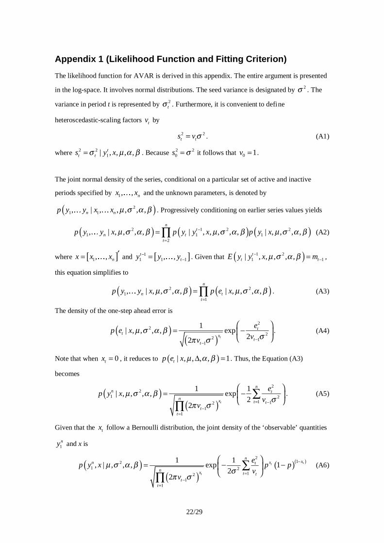
Appendix 1 (Likelihood Function and Fitting Criterion)
The likelihood function for AVAR is derived in this appendix. The entire argument is presented
in the log-space. It involves normal distributions. The seed variance is designated by 2σ . The
variance in period t is represented by 2tσ . Furthermore, it is convenient to define
heteroscedastic-scaling factors tv by
2 2t ts v σ= . (A1)
where 2 21| , , , ,t
t ts y xσ µ α β= . Because 2 20s σ= it follows that 0 1v = .
The joint normal density of the series, conditional on a particular set of active and inactive
periods specified by 1, , nx xK and the unknown parameters, is denoted by
( )21 1, | , , , , ,n np y y x x µ σ α βK K . Progressively conditioning on earlier series values yields
( ) ( ) ( )2 1 2 21 1 1
2
, | , , , , | , , , , , | , , , ,n
tn t
t
p y y x p y y x p y xµ σ α β µ σ α β µ σ α β−
=
= ∏K (A2)
where [ ]1, , nx x x ′= K and [ ]11 1 1, ,t
ty y y−−= K . Given that ( )1 2
1 1| , , , , ,tt tE y y x mµ σ α β−
−= ,
this equation simplifies to
( ) ( )2 21
1
, | , , , , | , , , ,n
n tt
p y y x p e xµ σ α β µ σ α β=
= ∏K . (A3)
The density of the one-step ahead error is
( )( )
22
22 1
1
1| , , , , exp
22t
tt x
tt
ep e x
vvµ σ α β
σπ σ −−
= −
. (A4)
Note that when 0tx = , it reduces to ( )| , , , , 1tp e x µ α β∆ = . Thus, the Equation (A3)
becomes
( )( )
22
1 21 12
11
1 1| , , , , exp
22
t
nn t
n x t tt
t
ep y x
vv
µ σ α βσ
π σ = −−
=
= −
∑
∏. (A5)
Given that the tx follow a Bernoulli distribution, the joint density of the ‘observable’ quantities
1ny and x is
( )( )
( )( )2
121 2
121
1
1 1, | , , , exp 1
22
tt
t
nxxn t
n x t tt
t
ep y x p p
vv
µ σ α βσ
π σ
−
=−
=
= − −
∑
∏ (A6)
23/29
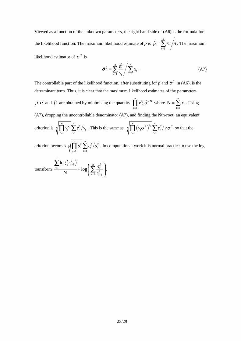
Viewed as a function of the unknown parameters, the right hand side of (A6) is the formula for
the likelihood function. The maximum likelihood estimate of p is 1
ˆn
tt
p x n=
= ∑ . The maximum
likelihood estimator of 2σ is
2
2
1 1
ˆn n
tt
t tt
ex
vσ
= == ∑ ∑ . (A7)
The controllable part of the likelihood function, after substituting for p and 2σ in (A6), is the
determinant term. Thus, it is clear that the maximum likelihood estimates of the parameters
,µ α and β are obtained by minimising the quantity 2N1
1
ˆt
nxt
t
v σ−=
∏ where 1
Nn
it
x=
= ∑ . Using
(A7), dropping the uncontrollable denominator (A7), and finding the Nth-root, an equivalent
criterion is 2N
11
t
n nxt t t
tt
v e v==
∑∏ . This is the same as ( )2 2 2N
11
tn nx
t t ttt
v e vσ σ==
∑∏ so that the
criterion becomes 2 2 2N
11
n n
t t ttt
s e s==
∑∏ . In computational work it is normal practice to use the log
transform ( )2
1 21
21 1
loglog
N
n
t nt t
t t
se
s
−=
= −
+
∑∑ .

24/29
Appendix 2 (Monthly Demand Data for Three Car Parts) M
onth
Par
t
Yea
r
1 2 3 4 5 6 7 8 9 10 11 12
1 1 3 0 2 0 0 0 0 1 0 0 1 2
2 0 1 0 0 1 1 2 1 0 2 0 0
3 0 1 1 2 2 2 1 0 0 2 0 0
2 1 8 5 1 2 3 4 4 1 1 0 1 5
2 4 1 5 2 0 1 1 3 1 1 1 1
3 0 0 1 2 1 0 0 1 0 0 1 1
3 1 64 59 65 73 74 86 68 40 35 66 97 64
2 75 54 25 70 48 68 64 35 35 26 51 51
3 27 48 25 60 26 41 32 37 57 23 39 21
25/29
Method GAM SES MCROST LOG AVAR
y 0.78
$m0 0.78 1.56 0.37 0.37
$m36 0.78 1.56 0.37 0.37
$α 0 0 0 0
$β 0.15
$σ 2 0.79 0.78 0.36 0.14
0v̂ 0.28
36v̂ 0.13
$p 0.5 0.5 0.5
Pr yt < 0
0.18 0.00
S 7.2 5.9 6.0 6.2 6.4
Table 1. Summary of Results for Car Part 1
26/29
Method GAM SES MCROST LOG AVAR
y 1.75
$m0 4.08 4.01 1.07 1.12
$m36 0.66 1.19 0.14 0.11
$α 0.24 0.22 0.19 0.21
$β 0.30
$σ 2 1.85 2.79 2.94 0.43
0v̂ 0.87
36v̂ 0.08
$p 0.78 0.78 0.78
Pr yt < 0
0.35 0.18
S 15.0 11.8 12.0 10.0 6.1
Table 2. Summary of Results for Car Part 2

27/29
Method GAM SES MCROST LOG AVAR
y 50.81
$m0 64.80 64.80 4.15 4.15
$m36 35.04 35.04 3.50 3.50
$α 0.20 0.20 0.19 0.19
$β 0.00
$σ 2 19.40 292 292 0.14
0v̂ 0.08
36v̂ 0.08
$p 1 1 1
Pr yt < 0
0.02 0.02
S 251 207 204 189 169
Table 3. Summary of Results for Car Part 3

C:\data\research\nonneg\Forecasting Sales of Slow and Fast Moving Inventories04 06/07/2001
Car Part 1
0
1
2
3
41 5 9 13 17 21 25 29 33
Months
Car Part 2
0
2
4
6
8
1 5 9 13 17 21 25 29 33
Months
Car Part 3
20
40
60
80
100
1 5 9 13 17 21 25 29 33
Months
Figure 1. Demand Series for Car Parts

29/29
Car Part 1
00.5
11.5
22.5
33.5
1 5 9 13 17 21 25 29 33
Months
Car Part 2
0
2
4
6
8
1 5 9 13 17 21 25 29 33
Months
Car Part 3
20
40
60
80
100
1 5 9 13 17 21 25 29 33
Months
Figure 2. Demand Series (solid line) and AVAR Smoothed Series (dashed line)