Forecasting Global Rice Consumption

Roderick M. Rejesus*, Samarendu Mohanty†, and Joseph V. Balagtas‡

Corresponding Author:

Roderick M. Rejesus Department of Agricultural and Resource Economics

North Carolina State University NCSU Box 8109

Raleigh, NC 27695-8109

Phone No.: 919-513-4605 Fax No.: 919-515-1824

E-mail: rod_rejesus@ncsu.edu

March 20, 2012

* Roderick M. Rejesus is Associate Professor, Department of Agricultural and Resource Economics, North Carolina State University, Raleigh, NC 27695-8109 † Samarendu Mohanty is Head, Social Sciences Division and Program Leader- Targeting and Policy, International Rice Research Institute, Los Baños, Laguna, Philippines ‡ Joseph V. Balagtas is Associate Professor, Department of Agricultural Economics, Purdue University, West Lafayette, IN 47907-2056

ii

Forecasting Global Rice Consumption

ABSTRACT

This paper examines the time-series properties of global rice consumption data commonly used in studies of consumption trends and evaluates alternative time-series models for long-range forecasts. Using time-series data from 1961-2011, we find that per capita rice consumption and GDP per capita are non-stationary in levels (i.e., they are unit root processes) and are not cointegrated. Thus previous studies that have applied econometric models for stationary data suffer from the well-known spurious regression problem. Out-of-sample performance evaluation of appropriate, univariate time-series forecasting methods suggest that double exponential smoothing may be the preferred approach to forecast global rice consumption. Our forecast results suggest that global rice consumption is projected to increase from 450 million tons in 2011 to about 490 million tons in 2020, and to about 650 million tons by 2050. Moreover, forecast intervals for these point estimates tend be very wide (especially in 2050), reflecting the inherent uncertainty in making long-run forecasts using any approach. These wide forecast intervals suggest a great deal of caution is appropriate when interpreting such forecasts for formulating public policy. Keywords: Consumption, Demand, Food Security, Forecasting, Rice, Time-series Analysis, Unit

Roots JEL Classification: Q10, Q11, Q18

1

Forecasting Global Rice Consumption

Introduction

Rice is the major staple crop of nearly half of the world’s population, and is particularly important in

Asia, where approximately 90% of world’s rice is produced and consumed (Zeigler and Barclay, 2008;

Khush, 2004). Global rice production has tripled in the last five decades from 150 million tons in 1960 to

450 million tons in 2011, thanks in large part to the rice Green Revolution in Asia. Since the introduction

of high yielding semi-dwarf varieties in 1960s by the International Rice Research Institute (IRRI) more

than 1000 modern rice varieties have been released to farmers in many Asian countries, resulting in a

rapid increase in rice yields and global rice production. Global production dropped sharply at the

beginning of the 21st Century, from 410 million tons in 2000 to 378 million tons in 2003 because of

severe droughts in parts of Asia, but has recovered by growing 50 million tons between 2005 and 2011.

Rice is a staple food commodity with inelastic demand (Mohanty, Wailes and Chavez, 2010), and

with historically inadequate storage infrastructure in most developing countries in Asia (Rolle, 2011).

Thus trends in global rice consumption largely follow those in global production, rising steadily over the

last five decades (Figure 1). However population growth has outpaced growth in rice production, such

that per capita production, and thus per capita consumption, appears to have plateaued starting around

1990 at around 65 kg per year (Figure 2). Because demand is highly inelastic, reductions in aggregate

production result in large price increases and consumer welfare losses (See Figure 3 and Wright, 2011 p.

35). Also, because rice is a staple food that accounts for a large share of income for a large segment of the

world’s poor, price increases like the one experienced in 2007-2008 may have large income effects,

reducing income available for other needs (see Wood, Nelson, and Noguiera, 2012 for an application of

this principle to staple foods in Mexico). Thus, production and consumption trends in rice markets have

important implications for poverty, food security, and economic development, especially in Asia.

It is for this reason that previous work has sought to forecast global rice consumption. This

important literature seeks to provide information useful for resource allocation by producers, governments

and aid agencies, and is at the core of food security issues (Timmer, Block, and Dawe 2008, p.140). In

2

this paper we evaluate that literature and propose alternative forecast methods with qualitatively different

findings. We begin by summarizing key contributions of the extant research and identifying potential

conceptual and empirical limitations. We briefly discuss limitations of available data for assessing trends

in global rice demand. Then, taking the data as given, we turn to the development of appropriate

econometric models for forecasting rice consumption.

Previous Analyses of Global Rice Consumption: Findings and Limitations

A number of previous studies analyze and forecast global rice consumption using the global rice

consumption data plotted in Figure 1. A common prediction across these studies is that global rice

consumption will fall in the medium or long term. This prediction is based on the recent downturn in per

capita rice consumption shown in Figure 2, and the observed decreases in per capita rice consumption in

wealthy East Asian countries like Japan, Taiwan, and South Korea. For example, Timmer, Block, and

Dawe (2010) estimate a per capita rice consumption equation (in natural logarithm form) that is quadratic

in GDP, then use this estimated relationship and projections of global GDP to forecast global rice

consumption. Timmer, Block, and Dawe (2010) find that global rice consumption will increase modestly

until 2025 before declining rapidly to approximately 360 million tons by 2050.

Abdullah, Ito, and Adhana (2005) similarly use the USDA data on per capita consumption

(Figure 2) to project a range of scenarios for per capital rice consumption through 2050, all of which

forecast reductions in per capita consumption. Two of Abdullah, Ito, and Adhana’s (2005) three scenarios

forecast per capita consumption in Asia to drop sufficiently to cause aggregate Asian rice consumption to

decrease by 2050, despite continued population growth. The forecast model behind these projections is

not entirely clear, but the authors state that they assume a continuation of observed trends in per capita

consumption, and that per capita consumption in developing nations will decline based on the experience

in relatively wealthy, East Asian countries.

Rosegrant et al. (2001) project declining per capita consumption but rising aggregate

consumption of rice through 2020. While they do not provide model details behind these projections, like

3

Timmer, Block, and Dawe (2010) and Abdullah, Ito, and Adhana (2005), they argue that income growth

and rising urbanization will result in declining per capita consumption.

In contrast, Seck et al. (2012) project that global rice consumption will rise to 496 million tons in

2020 and further increase to 555 million tons by 2035. Seck et al. (2012) explain that aggregate global

rice consumption is still expected to increase through 2035 due to increased demand in Africa, Latin

America and parts of Asia, despite continued declines in per capita consumption in China and India (and

other wealthy Asian countries).

The role of income growth assumed by all of these studies and, more broadly, their projections of

per capita and aggregate rice consumption require additional inspection for several reasons. First, it is

well established that income elasticities for staple foods tend to decrease as incomes rises. However,

evidence on the income elasticity of demand for rice is mixed, with some studies finding negative income

elasticies for key countries (e.g., Ito, Peterson, and Grant 1989, 1991) and others arguing that such

estimates are understated or finding larger and positive income elasticies (Huang, David, and Duff , 1991;

Taniguchi and Chern, 2000; Chern et al., 2002). Moreover, many studies in this literature suffer from

serious limitations, including a misattribution of unobserved structural changes to income effects (Huang

and Bouis, 1996).

Second, the extant research on aggregate rice consumption typically lacks appreciation for

changes in supply. Data on global or national rice consumption is typically calculated as availability, that

is, production minus net changes in stocks and trade. Because consumption data tracks production very

closely, studies of rice demand using aggregate rice consumption data are not likely to yield unbiased

estimates of structural demand parameters in the absence of a careful econometric identification strategy

(Yu et al., 2004).

Third, global rice consumption figures also mask important differences in rice consumption

across regions, across countries, and across demographic groups within countries (Seck et al., 2012). For

example, while per capita rice consumption has decreased in high-income and middle-income Asian

countries (such as Japan and China), per capita rice consumption has continued to increase in Africa,

4

Latin America, and other Asian countries (IRRI, AfricaRice, CIAT, 2010). In addition, per capita

consumption of rice in developed regions like the United States and the European Union, as well as in

Middle Eastern countries, continues to grow (Seck et al., 2012). Given this heterogeneity in rice

consumption, any empirical relationship between global rice consumption and, say, global income or

price, in fact reflects an amalgam of the underlying, heterogeneous relationships, and may suffer from

aggregation bias that makes the estimated relationships problematic for inference, including forecasting

global consumption.

Finally, time series data on global and national consumption may be nonstationary. The extant

literature on global consumption ignores this possibility and analyzes the data under the assumption that

they are stationary. If this assumption is violated, the models used by Timmer, Block, and Dawe (2010),

Abdullah, Ito, and Adhana (2005), and others may be mis-specified and lead to erroneous inference. In

rest of this paper we put aside our reservations of using the global rice consumption data in order to focus

on the issue of nonstationarity. We first apply a battery of tests to assess the time-series characteristics of

the data. Then, based on these results, we explore appropriate econometric models.

Data and Preliminary Tests of Time-series Properties

The global rice consumption data used in this study (1961-2011) are from the USDA Production, Supply

and Demand online database, which is based primarily on the supply disappearance balance sheets for the

different rice-producing countries. At the country level the consumption variable is a residual or

availability measure calculated from the following identity: Beginning Stock + Production + Imports =

Ending Stock + Consumption + Exports. Our data on population (total and agricultural), GDP, and rice

export prices is the same as that used by Timmer, Block, and Dawe (2010) for 1960-2009, which we

updated to include the most recent available information. Recent population data are primarily from the

FAOSTAT online database which is primarily based on the United Nations World Population Prospects

(i.e., 2004 and 2010 revisions). Updated GDP figures are in constant US$ for year 2000 and were

collected from the World Development Indicator Online 2012. Updated rice export prices were taken

5

from the IRRI World Rice Statistics collection and these prices were deflated to reflect constant year 2000

US$ using deflators from World Development Indicator Online 2012. Consumption per capita and GDP

per capita figures were calculated by simply dividing the total consumption and GDP variables with the

corresponding total population data. Agricultural population share is computed by dividing the global

agricultural population with the total population.

A crucial first step in regression analysis of time-series data is to examine the data for the

presence of unit roots (e.g., Diebold and Kilian 2000). Least squares estimators of data with unit roots

may suffer from the well-known spurious regression phenomenon (Granger and Newbold, 1974; Phillips,

1986, 1987). In this case, a statistically significant relationship may be found between two variables with

unit roots even where no meaningful economic relationship exists. Thus we first test for unit roots in the

data on per capita rice consumption and per capita GDP. We apply a number of standard statistical tests

that have been developed over the past three decades to evaluate whether a time-series have a unit root

(and is therefore non-stationary). We use the Augmented Dickey-Fuller test (Dickey and Fuller, 1979),

Augmented Dickey-Fuller Generalized Least Squares (ADF-GLS) test (Elliot, Rothenberg, and Stock,

1996), the Phillips-Perron test (Phillips and Perron, 1988), and the KPSS (Kwiatkowski et al., 1992) test.

In all of these tests we allow for a deterministic time trend and an intercept. In the Augmented Dickey-

Fuller, ADF-GLS, and Phillips-Perron test, the null hypothesis is that the series is not stationary (i.e., unit

root is present). In contrast, the null hypothesis for the KPSS test is that the series is stationary (i.e., no

unit root present) and failure to reject the null hypothesis suggests the data are stationary.

We report results from unit root tests on per capita consumption and per capita GDP, 1960-2011,

in Table 1.1 All the tests indicate that unit roots may be present for both variables. In the Augmented

Dickey-Fuller, ADF-GLS, and Phillips-Perron tests, the test statistics are less than the 5% critical values

for both the per capita consumptions and GDP per capita variables. Therefore we fail to reject the unit

root hypothesis. For the KPSS test, the test statistic is greater than the 5% critical value for the two

1 The unit root tests presented in Table 1 accounts for a trend and an intercept. But we also implemented unit root tests that do not include a trend or do not include an intercept, and results of the tests still support the presence of unit roots. Results of these other forms of unit root tests are available from the authors upon request.

6

variables considered, such that we reject the null hypothesis of no unit root. Also, although not reported

here, unit root tests were also conducted for related variables used in the extant literature, namely export

price and the agricultural population share. The unit root tests for these variables and of log

transformations of these variables also support the presence of unit roots.

Given that per capita rice consumption and per capita GDP have unit roots, there is one case

where using these two variables in a classical regression framework would still be appropriate.

Specifically, if per capita consumption and per capita GDP are cointegrated then least squares estimation

of the regression of consumption on income yields superconsistent estimates of the long-run equilibrium

relationship between the two (Stock 1984). We use the Engle-Granger test (Engle and Granger, 1987) and

the Johansen test (Johansen, 1995) to test for cointegration between per capita consumption and per capita

GDP. The null hypothesis in these tests is that the variables examined are not cointegrated. We report

results of the cointegration tests in Table 2. All of the cointegration tests indicate that per capita rice

consumption and GDP per capita are not cointegrated. Test statistics are all below the 5% critical values

such that we fail to reject the null hypothesis of no cointegration.2

The presence of unit roots in per capita rice consumption and per capita GDP, together with our

finding that these variables are not cointegrated, suggest that least squares estimates of the regression of

per capita consumption on per capita GDP are spurious. That is to say, the estimated regression cannot be

interpreted as causal or, indeed, as having any economic meaning. Thus, the models used by Timmer,

Block, and Dawe (2010) and and others are mis-specified, and inference from these models is suspect.

We now turn to appropriate econometric techniques for evaluating these data and, in particular, using

them to forecast rice consumption.

Empirical Approach: Alternative Forecasting Models

First Differenced (FD) Regression Models

2 Although not presented here, pairwise cointegration tests for rice consumption per capita and rice export price, as well as consumption per capita and agricultural population share, also weigh against cointegration.

7

In the presence of unit roots and no cointegration, one alternative approach is to first difference the

variables in the regression specification and then estimate the parameters in the model by OLS (Greene,

2008; Wooldridge, 2009). If the estimated parameters in the regression are statistically significant, then

the first difference model can be used for forecasting per capita rice consumption. If all of the estimated

parameters from the first differenced (FD) model are not significant, then the specification used in the

regression is not useful for forecasting (i.e., the right-hand side variables do not help determine per capita

rice consumption behavior). In the case above, alternative models like univariate time-series approaches

(i.e., time-series regression models using past/lagged values to predict future values) may be more

informative in terms of forecasting future per capita rice consumption.

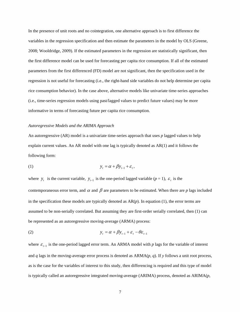
Autoregressive Models and the ARIMA Approach

An autoregressive (AR) model is a univariate time-series approach that uses p lagged values to help

explain current values. An AR model with one lag is typically denoted as AR(1) and it follows the

following form:

(1) ttt yy εβα ++= −1 ,

where ty is the current variable, 1−ty is the one-period lagged variable (p = 1), tε is the

contemporaneous error term, and α and β are parameters to be estimated. When there are p lags included

in the specification these models are typically denoted as AR(p). In equation (1), the error terms are

assumed to be non-serially correlated. But assuming they are first-order serially correlated, then (1) can

be represented as an autoregressive moving-average (ARMA) process:

(2) 11 −− −++= tttt yy θεεβα

where 1−tε is the one-period lagged error term. An ARMA model with p lags for the variable of interest

and q lags in the moving-average error process is denoted as ARMA(p, q). If y follows a unit root process,

as is the case for the variables of interest to this study, then differencing is required and this type of model

is typically called an autoregressive integrated moving-average (ARIMA) process, denoted as ARIMA(p,

8

d, q) where d is the number of times the variable is differenced. When a series has a unit root, first-

differencing (d = 1) is typically sufficient to achieve stationarity and this first-differencing approach is

used in this study. Hence, an ARIMA(1,1,1) model is equation (2) above with yt and yt-1 replaced by the

first differences.

A practical issue in estimating ARIMA models is the choice of p and q. One approach for

choosing p is by estimating sequentially higher-order models (p = 1, 2, 3, and so on) and selecting the

model for which the parameter estimate associated with the last lagged variable is significant. For

example, if an AR(1) and an AR(2) model is estimated and the parameter estimated with the first lag is

statistically significant in both models but the second lag is insignificant in the AR(2) model, then we

choose p = 1. Autocorrelation tests on the model with the optimal p can then indicate the q lags to use.

Thus, if autocorrelation is not present in the AR(1) example above, then q = 0. An ARIMA(1,1,0) model

would be appropriate in this case.

Alternatively p and q in an ARIMA model may be chosen on the basis of autocorrelation and

partial autocorrelation function (ACF and PACF) graphs, in the so-called Box-Jenkins model

identification process (Box and Jenkins, 1970). In this approach, the number of lags in the AR process is

based on the PACF graph where the choice of p is where the PACF becomes zero (or is close to zero) at

(p + 1) lags, and the choice of q lags in the MA process is chosen such that the ACF becomes zero at (q +

1) lags.

In this study, we use the two approaches above to choose the p and q for the ARIMA model. If

the chosen ARIMA model is different using the two approaches above, we look at the statistical

significance of the lagged AR and MA terms to determine which ARIMA model to use in forecasting per

capita rice consumption.

Double Exponential and Holt-Winters Smoothing Approaches

The ARIMA model above is just one univariate time-series approach that can be used in forecasting per

capita rice consumption. We also use exponential smoothing approaches that are in the class of adaptive-

9

forecasting algorithms used for forecasting. Exponential smoothing is a univariate forecasting technique

that give allots greater weight to more recent observations, and exponentially decreasing weights to

observations further in the past. This is in contrast with the simple ARMA estimates that implicitly grant

equal weights for all time-series observations.

There are three kinds of exponential smoothing methods: single exponential, double exponential,

and the Holt-Winters. These exponential smoothing methods can be interpreted as special cases of either

ARIMA(0, 1, 1) or ARIMA(0, 2, 2) and imply an inherent differencing that addresses the non-stationarity

issue in our data (Gardner, 1985; Chatfield, 2005). In the single exponential method, for any time t, the

smoothed or forecasted value St is computed by using the following equation:

(3) 1)1( −−+= ttt SyS αα for t = 1, …, T

where yt is the current observation, α is a smoothing parameter, and S0 is the initial value. Equation (3) is

the adaptive forecasting form of the single exponential smoother. With continuous substitution of 1−tS

equation (3) can be re-written as a weighted moving-average with geometrically decreasing weights:

(4) 0

1

0)1()1( SyS T

KT

T

k

Kt ααα −+−= −

−

=∑ .

Equation (4) illustrates the exponential behavior of this smoothing method. The smoothing parameter α

determines how quickly the older responses are dampened. If α is close to 1 dampening is quick and if

α is close to zero dampening is slow. In this study, the value of α is estimated by minimizing the in-

sample mean squared forecast error through a bisection method.

The limitation of a single exponential smoothing in forecasting is that it only provides a single

value for the entire forecast horizon (i.e., one single out-of-sample forecast for all steps ahead).

Graphically a single value forecast is represented by a horizontal line in the forecast horizon. This makes

single exponential smoothing appropriate only for time-series data that exhibit no linear or higher-order

trends. Since rice consumption is trending upwards over time (See Figures 1 and 2), a single exponential

method may not be suitable for the purpose of this study. If the time-series variable of interest has a trend,

then the double exponential or the Holt-Winters smoothing method may be more appropriate.

10

In double exponential smoothing, the smoothed series in (3) is again smoothed such that:

(5) ]2[1

]2[ )1( −−+= ttt SSS αα .

Values of 0S and ]2[0S are necessary to begin the process in (5). To obtain the initial values 0S and ]2[

0S

the following equations are utilized:

(6a) ( ){ } 100ˆ/1ˆ βααβ −−=S

(6b) ( ){ } 10]2[

0ˆ/12ˆ βααβ −−=S .

The coefficients 0β̂ and 1β̂ are estimated by OLS using the following model: tyt 10 ββ += . As with the

single exponential approach, the smoothing parameter α is found by minimizing the in-sample mean

squared forecast error. For forecasting values out of sample, the τth-step ahead forecast is calculated

using:

(7) TTt bay ττ +=+ˆ

Where the constant term is ]2[2 TTT SSa −= and the linear term is ( )]2[1 TTT SSb −= −αα . Based on (7), the

out-of-sample predictions would not be constant (as in the single-exponential case).

The Holt-Winters smoothing approach is the most general among the three smoothing methods

discussed in this section because it can accommodate both trends and seasonality in the time-series (Holt,

2004; Winters, 1965). In our case, there is no evidence of seasonality given the plots in Figures 1 and 2.

Hence, the most general Holt-Winters method that account for seasonality is not considered in this study.

In the non-seasonal Holt-Winters smoothing, the τth-step-ahead forecast can be calculated using the

following formula:

(8) ttt bay ττ +=+ˆ .

The ta and tb terms in (8) are calculated using the following updating equations:

(9a) ))(1( 11 −− +−+= tttt baya αα ,

(9b) 11 )1()( −− −+−= tttt baab ββ ,

11

where α and β are two smoothing parameters. Starting values 0a and 0b are required to begin the

process in (9a) and (9b). These initial values are estimating the following regression model by OLS:

tbayt 00 += . The smoothing parameters are chosen by minimizing the in-sample penalized sum-of-

squared forecast errors. The penalty term included in this optimization criterion helps to achieve

convergence when one of the parameters is close to the boundary conditions. Note that the Holt-Winters

approach is still more general than the double exponential method because this procedure allows the ta

and tb terms in (8) to change over time.

Out-of-Sample Forecast Evaluation: RMSE, MAE, and the Diebold-Mariano Test

In the discussion above, we present three potential methods that may be used to model our rice

consumption data and allow us to forecast future rice consumption – the ARIMA model, double

exponential smoothing, and Holt-Winters smoothing. We use the root mean square error (RMSE)

criterion, the mean absolute error (MAE) criterion, and the Diebold-Mariano test of predictive accuracy

(Diebold and Mariano, 1995) to evaluate the out-of-sample forecasting accuracy of these three forecasting

models. These tests allow us to choose the best approach to forecast rice consumption at different forecast

horizons (i.e., for 5-year, 10-year, and 20-year forecasts). Out-of-sample forecast evaluation is conducted

by splitting the time-series data such that the last 5-years (T - 5), the last 10-years (T - 10), and the last 20-

years (T - 20), respectively, are left out of the estimating sample and forecasted values for these periods

are compared to the actual observed values to assess forecast accuracy. For example, if we have time-

series data from 1961-2011 and we are interested in doing an out-of-sample evaluation for a 5-year

forecast horizon, then the time series will be split such that the data from 1961-2006 (46 years) will be

used to estimate the parameters, and the remaining actual data (2007-2011) will be used to compare it

with the forecasted values. The same splitting process is used for the 10-year and 20-year forecast

horizons.

Suppose that we have n + m total time-series observations such that (n + m = T). Further assume

that we use the first n observations to estimate the parameters of a forecasting model and save the last m

12

observations for prediction/forecasting. Let hnf +ˆ be the forecast for the saved m observations such that h

= 1, …, m. The m forecast errors can then be defined as: hnhnhn fye +++ −= ˆˆ . The RMSE can then be

calculated as:

(10) 21

1

1 ˆ

= ∑

=+

−m

hhnemRMSE .

The MAE can also be calculated as follows:

(11) ∑=

+−=

m

hhnemMAE

1

1 ˆ .

We prefer a forecasting approach with lower RMSE or MAE.

An analyst would prefer a forecast model with lower RMSE and MAE, but the question remains

whether RMSE or MAE for competing models are statistically different? Diebold and Mariano (1995)

addressed this issue by developing the Diebold-Mariano (DM) test of predictive accuracy. Given an

actual time series and two competing forecast methods, one may apply a loss function (either a squared

error or absolute error) and then calculate test statistics of predictive accuracy that allows the null

hypothesis of equal accuracy to be tested. Specifically, the DM test statistic allows one to test whether the

mean difference between the loss functions for the two forecast methods is zero, using a long-run estimate

of the variance of the difference series. Since the DM tests allows comparison of two forecast methods at

a time, we use pair-wise comparisons to compare the forecast methods considered in this study (i.e.,

double exponential vs. Holt-Winters, double exponential vs. ARIMA, and Holt-Winters vs. ARIMA).

Results and Discussion

First Difference (FD) Models

Table 3 presents the parameter estimates from three first-differenced models examined in this study.

Model (1) in Table 3 only includes first-differenced GDP per capita, Model (2) adds a first-differenced

one-period lagged rice export price and first-differenced agricultural population share, and Model (3)

further adds a linear trend (Year). The specifications used in Table 3 are first-differenced versions of the

13

specifications used by Timmer, Block, and Dawe (2010), whose model in levels is inappropriate due to

the presence of unit roots. We do not include any quadratic terms for the first-differenced GDP per capita

because the time series plots of the first-differenced variables do not exhibit behavior consistent with this

specification. The key finding in Table 3 is that none of the parameters is statistically different from zero.3

In other words, GDP, export price, and the agricultural population are not helpful for explaining or

forecasting rice consumption. Therefore we turn our attention to univariate forecasting methods

appropriate for unit-root processes.

Results of the Autoregressive Models, ARIMA Models, and Smoothing Methods

In Table 4 we report the parameter estimates for AR(1) and an AR(2) models of the first-differenced per

capita rice consumption variable. The parameter estimate associated with the one period lagged variable

was statistically significant at the 10% level in both the AR(1) and AR(2) models. However, the second

period lagged variable is not statistically significant in the AR(2) model. There is also evidence of

autocorrelation in the AR(2) model, but none in AR(1). Based on these findings, an ARIMA(1, 1, 0)

model is one candidate for forecasting global rice consumption through 2050.

ACF and PACF plots of first-differenced per capita rice consumption are presented in Figures 7

and 8, respectively. Although all the spikes in both the ACF and PACF graphs are within the 95%

confidence bands, the ACF moves closer to zero from the 4th lag and the PACF moves closer to zero at

the 3rd lag. Therefore, q = 3 and p = 2 may be the appropriate lag numbers to use for the MA and AR

process of an ARIMA forecasting model. An ARIMA(2, 1, 3) model may then be another candidate

model for forecasting global rice consumption.

We report parameter estimates for the ARIMA(1, 1, 0) and ARIMA(2, 1, 3) models in Table 5.

The AR(1) parameter estimate is strongly statistically significant in the ARIMA(1, 1, 0) model. In the

ARIMA(2, 1, 3) model, only the MA(3) term was statistically significant and only at the 10% level.

3 Estimates of the models specified in first differences of the natural logs yields the same results: none of the estimates are statistically significantly different from zero.

14

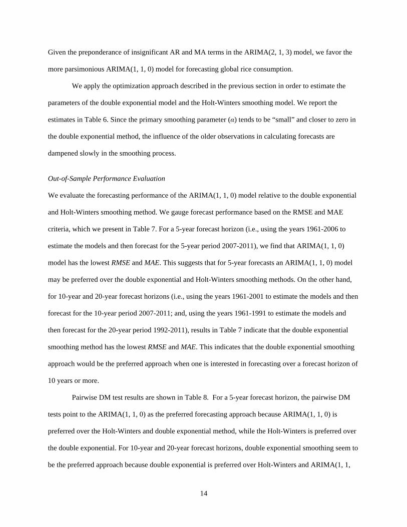
Given the preponderance of insignificant AR and MA terms in the ARIMA(2, 1, 3) model, we favor the

more parsimonious ARIMA(1, 1, 0) model for forecasting global rice consumption.

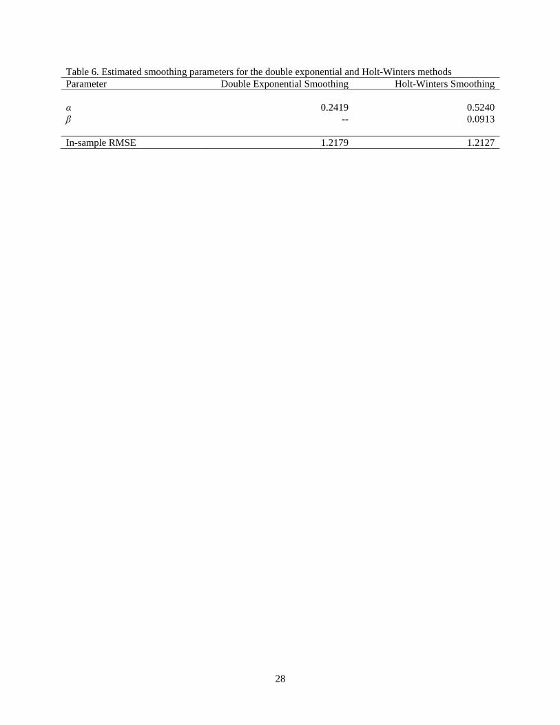
We apply the optimization approach described in the previous section in order to estimate the

parameters of the double exponential model and the Holt-Winters smoothing model. We report the

estimates in Table 6. Since the primary smoothing parameter (α) tends to be “small” and closer to zero in

the double exponential method, the influence of the older observations in calculating forecasts are

dampened slowly in the smoothing process.

Out-of-Sample Performance Evaluation

We evaluate the forecasting performance of the ARIMA(1, 1, 0) model relative to the double exponential

and Holt-Winters smoothing method. We gauge forecast performance based on the RMSE and MAE

criteria, which we present in Table 7. For a 5-year forecast horizon (i.e., using the years 1961-2006 to

estimate the models and then forecast for the 5-year period 2007-2011), we find that ARIMA(1, 1, 0)

model has the lowest RMSE and MAE. This suggests that for 5-year forecasts an ARIMA(1, 1, 0) model

may be preferred over the double exponential and Holt-Winters smoothing methods. On the other hand,

for 10-year and 20-year forecast horizons (i.e., using the years 1961-2001 to estimate the models and then

forecast for the 10-year period 2007-2011; and, using the years 1961-1991 to estimate the models and

then forecast for the 20-year period 1992-2011), results in Table 7 indicate that the double exponential

smoothing method has the lowest RMSE and MAE. This indicates that the double exponential smoothing

approach would be the preferred approach when one is interested in forecasting over a forecast horizon of

10 years or more.

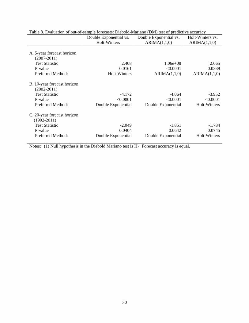
Pairwise DM test results are shown in Table 8. For a 5-year forecast horizon, the pairwise DM

tests point to the ARIMA(1, 1, 0) as the preferred forecasting approach because ARIMA(1, 1, 0) is

preferred over the Holt-Winters and double exponential method, while the Holt-Winters is preferred over

the double exponential. For 10-year and 20-year forecast horizons, double exponential smoothing seem to

be the preferred approach because double exponential is preferred over Holt-Winters and ARIMA(1, 1,

15

0), while the Holt-Winters procedure is preferred over ARIMA(1, 1, 0). These DM test results are

consistent with the RMSE and MAE analysis such that the ARIMA(1, 1, 0) model is the preferred method

for short-run forecasting of global per capita rice consumption, while the double exponential method is

preferred for forecasting over horizons of 10 years or more. Thus, we mainly use the double exponential

method for forecasting global rice consumption because we are interested in a long-run forecast through

2050.

Global Rice Consumption Forecasts from the Double Exponential Smoothing Method

Figure 6 shows the actual values, the point forecasts, and the 95% forecast intervals of per capita rice

consumption based on the double exponential smoothing method.4 Our point forecast indicates continued,

gradual increase in per capita consumption. Combining our forecasts of per capita consumption with

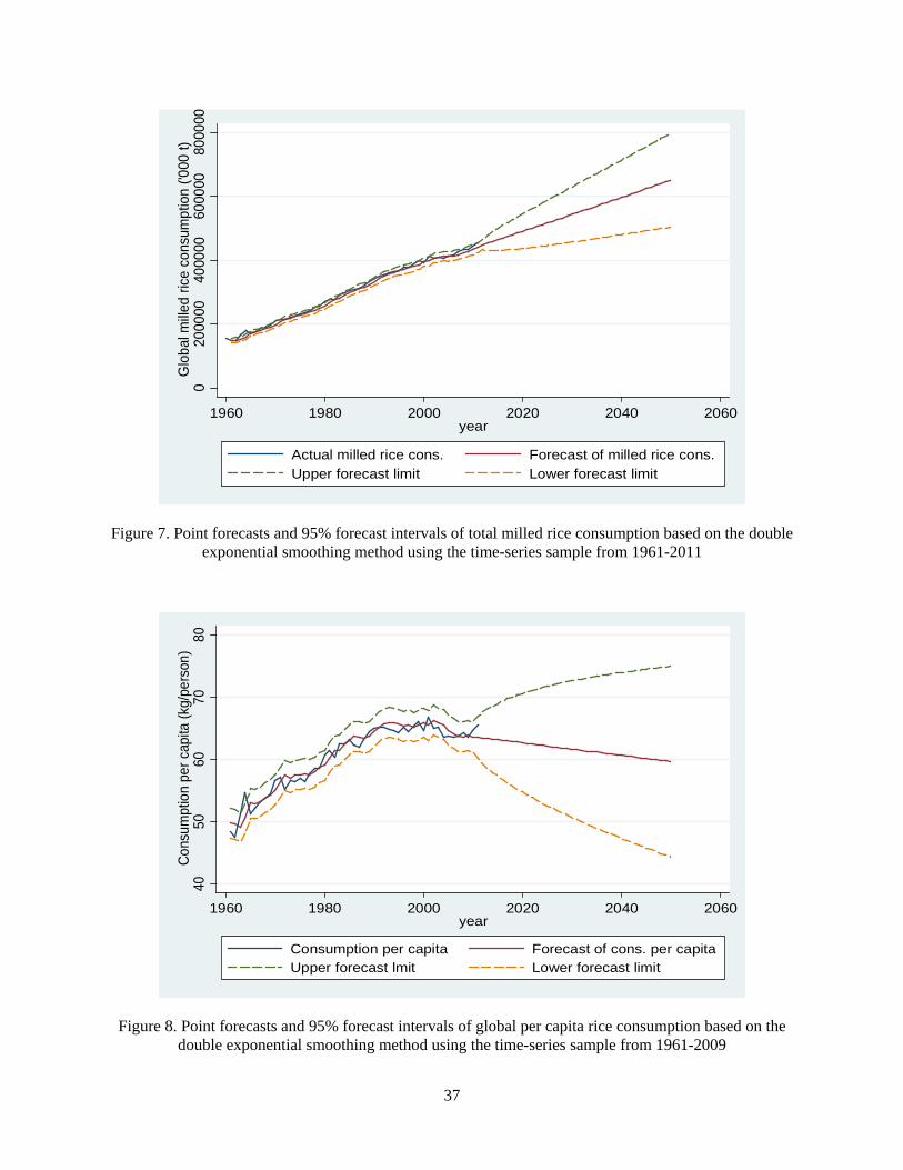
actual and forecasted values of global population through 2050, Figure 7 presents a graph of the actual

values, the point forecasts, and the forecast interval for total global rice consumption.5 In contrast to the

extant literature, we forecast both per capita consumption and total consumption to continue to rise. The

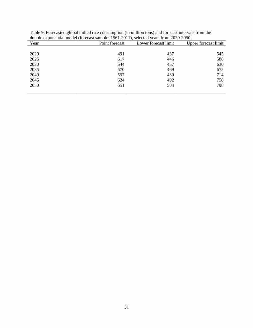
point forecast values and forecast interval values based on the double exponential method are presented in

Table 9 for selected years in the period 2020-2050. The double exponential forecasting approach indicates

that in 2020 total rice consumption would modestly increase from 450 million tons in 2011 to

approximately 491 million tons in 2020. By 2050, total rice consumption is forecasted to be

approximately 651 million tons.

We hasten to note that our forecasts, like most economic forecasts, are quite imprecise. In 2020,

the 95% forecast interval is between 437 million tons and 545 million tons; while in 2050, the forecast

4 A 95% forecast interval is used based on the following formula: h

tf σ96.1ˆ ± where

tf̂ is the point forecast, σ is

the forecast standard deviation, and h = 1, …, k for a k-period forecast horizon. Note that h =1 for the estimation sample. 5 A double exponential smoothing method is also used to forecast global population. Using this method, the global population is expected to increase from 6.9 billion in 2011 to about 9.8 million in 2050. Note that the forecast intervals for the total aggregate consumption do not account for the imprecision inherent in estimating the population forecasts. If this imprecision is accounted for, the calculated forecast intervals in Figures 7 and 9 would be wider. Hence, the forecast intervals shown in the aforementioned figures should be considered as conservative estimates of the bounds.

16

interval is between 504 million tons and 798 million tons. These wide forecast intervals reflect the

inherent imprecision of time-series forecasts of global rice consumption over a long forecast horizon.

Nonetheless it is notable that even the lower bound of our forecast interval is rising through 2050.

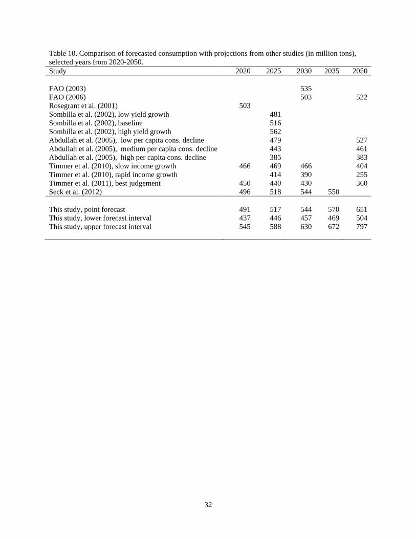
In Table 10, we compare our forecast results with recent studies that also forecasted global rice

consumption through particular years. In 2020, the available forecasts from Rosegrant et al. (2001),

Timmer, Block, and Dawe (2010), and Seck et al. (2012) are all within the forecast interval in our study

(i.e., between 437 to 545 million tons). In 2025, the forecasts from all of the scenarios in Sombilla,

Rosegrant, and Meijer (2002), the low per capita consumption decline scenario of Abdullah, Ito, and

Adhana (2005), the slow income growth scenario of Timmer, Block, and Dawe (2010), and forecasts

from Seck et al. (2012) are still within the forecast interval in our study (i.e., between 446 to 588 million

tons). The remaining scenario forecasts for 2025 tend to be below the lower bound of our forecast

interval. By 2050, only the forecast values from FAO (2006) and the high per capita consumption

scenario in Abdullah, Ito, and Adhana (2005) are within the forecast intervals of this study. The forecasts

from the other scenarios in Abdullah, Ito, and Adhana (2005) and all scenarios in Timmer, Block, and

Dawe (2010) are less than the lower bound of our 95% forecast intervals. Thus, compared to our

forecasts, much of the extant literature forecasts relatively low consumption by 2050.

Differences in rice consumption forecasts across studies might be explained in part by the use of

data spanning different time periods. For the forecasts plotted in Figure 6 we used data from 1961-2011.

However, if we had used data through 2009, as in Timmer, Block, and Dawe, 2010, our forecasts and the

inferences drawn from them would be very different. In Figure 8, we depict the point forecasts and

forecast intervals of per capita rice consumption using only data from 1961-2009. This shorter sample

omits the increases in per capita rice consumption observed in 2010 and 2011 (Figure 2). Hence, the

forecasts depicted in Figure 8 are lower than that in Figure 6, and indicate gradually declining per capita

consumption, as found by Timmer, Block, and Dawe (2010) and others. The resulting total global

consumption forecasts and forecast intervals when only using the 1961-2009 series are then shown in

Figure 9. Despite our forecast for declining per capita consumption, we find population growth proceeds

17

fast enough to maintain gradually increasing aggregate rice consumption. Even the lower bound of our

95% confidence band continues to rise through 2050.

Thus when we compare forecasts based on the same sample as Timmer, Block, and Dawe (2010),

we find qualitatively different results. Remaining differences in rice consumption forecasts, and in

particular the fact that many papers forecast declining global consumption while our model suggests

otherwise, result from different model specifications. In this case, it appears the failure of the extant

literature to diagnose and model unit roots in the data leads to faulty inference.

The forecast values and confidence bounds for selected years are presented in Table 11. In this

case, estimating the model on the 1961-2009 sample reduced the 2050 forecasts and corresponding

forecast intervals by approximately 40 to 50 million tons (relative to the values when we used the 1961-

2011 sample for estimation). These results illustrate the sensitivity of forecasts to the estimation sample

used. The smoothing approaches used in this study are especially affected by this sensitivity given that

these smoothing methods assign more weight to more recent observations compared to observations

farther in the past.

Conclusions and Policy Implications

Forecasting future global rice consumption is important for guiding producers, rice market participants,

policy-makers, and research donors in their decision-making. Information about trends in global rice

consumption would allow producers and other participants in the rice value-chain to know more about

how to effectively position their operations in the future. Policy-makers, researchers, and donor agencies

could use the information to formulate policies and allocate research investments.

This study aims to provide a better understanding of the time-series properties of global rice

consumption. Our starting point is to note a potentially important oversight in the existing research on

trends in global rice consumption: namely, that the time series data commonly used in such studies may

be characterized by unit root processes. If so, models in the existing research may be mis-specified. We

conduct formal tests for unit roots and cointegration and find that the time series data for global per capita

18

rice consumption, per capita GDP, and other variables associated with rice markets, are indeed

characterized by unit root processes, but are not cointegrated. Therefore, regression models commonly

used to analyze these data without properly dealing with the unit roots suffer from the spurious regression

problem, and should not be used to forecast rice consumption.

In light of this finding, we propose and compare the forecast performance of alternative models

appropriate for unit root processes. We estimate three univariate time-series forecasting techniques that

account for the unit root issue: double exponential smoothing, Holt-Winters smoothing, and ARIMA

models. Of these candidate methods, the double exponential smoothing procedure yields better out-of-

sample forecasts or global per capita consumption over a range of forecasting horizons.

Using the double exponential smoothing method, global rice consumption is projected to increase

to about 490 million tons in 2020 and to around 650 million tons by 2050. Our forecast for continued

consumption growth stands in stark contrast to previous work which forecasts consumption to begin to

decline by 2050, but which are based on mis-specified models.

Moreover, we note that the forecast intervals for these point forecasts tend be very wide and

increasing in the forecast time horizon: a 95% forecast interval for 2020 is between 437 and 545 million

tons, and the forecast interval for 2050 is between 504 to 797 million tons. Despite this wide interval the

2050 forecasts from previous studies tend to be lower than the lower end of our forecast bands.

We draw two implications of this analysis for the existing work on trends in global rice

consumption. First, inappropriate statistical models are yielding long-run (2050) consumption forecasts

that are likely to be too low, lower even than the lower limit of our 95% confidence band. Our best-guess

forecasts suggest gradually increasing per capita consumption and rising aggregate consumption through

2050 and beyond. Second, appropriate time-series forecasts of rice consumption using these data are

highly uncertain, and can differ dramatically based on the sample period used to estimate the model. Thus

policies and research investments based on point forecasts are likely to be misguided; policy-makers, aid

agencies, and donors would be well-advised to be aware of the inherent imprecision of such forecasts.

19

More generally, for reasons we discuss at the beginning of this paper, the global rice consumption

data used here and in previous work may be inappropriate for making inference on past consumption

trends or forecasting future consumption. Future research in this area should use data and methods that

account for heterogeneity in consumption across regions, countries, and demographic groups; and that

econometrically identify structural rice demand parameters (Yu et al., 2004). Longitudinal or panel

household survey data of rice consumption for various countries would likely provide better inferences

about the influence of income and other factors on rice demand and, based on parameters from these type

of models, improved rice consumption forecasts can be estimated.

20

References:

Abdullah A.B., S. Ito, K. Adhana. 2005. Estimate of rice consumption in Asian countries and the world towards 2050. Tottori University, Japan. p 28-42. Online: http://worldfood.apionet.or.jp/alias.pdf.

Bouis, H. 1991. “Rice in Asia: Is it becoming a commercial good?” American Journal of Agricultural

economics 73(2): 522-527. Box, G and G. Jenkins. 1970. Time-Series Analysis: Forecasting and Control. San Francisco, CA:

Holden-Day Press. 784 p. Chatfield, C. 2001. Time-Series Forecasting. London: Chapman & Hall/CRC. 280 p. Chern, W.S., K Ishibashi, K. Taniguchi, and Y. Tokoyama. 2002. “Analyis of food consumption behavior

by Japanese households.” ESA Working Paper No. 02-06. Available online at http://www.fao.org/docrep/007/ae025e/ae025e00.htm.

Dickey, D. and W. Fuller. 1979. “Distribution of the Estimators for Autoregressive Time Series with a

Unit Root.” J. of the Amer. Stat. Assoc. 74: 427-431. Diebold, F.X. and L. Killian. 2000. “Unit Root Tests are Useful for Selecting Forecasting Models.” J. of

Bus. and Econ. Stat. 18(3): 265-273. Diebold, F. and R. Mariano. 1995. “Comparing Predictive Accuracy.” J. of Bus. and Econ. Stat. 13(3):

253-263. Elliot, G., T. Rothenberg, and J. Stock. 1996. “Efficient Tests for an Autoregressive Unit Root.”

Econometrica. 64: 813-836. Engle, R.F. and C.W.J. Granger. 1987. “Cointegration and Error Correction: Representation, Estimation,

and Testing.” Econometrica. 55: 251-276. FAO (Food and Agriculture Organization). 2003. World agriculture: towards 2015/2030. Summary

report. Online: http://www.fao.org/docrep/004/y3557e/y3557e00.htm#TopOfPage. FAO (Food and Agriculture Organization). 2006. World agriculture: towards 2030/2050. Interim report.

Global Perspectives Study Unit. Rome, Italy. Online: http://www.fao.org/es/esd/AT2050web.pdf. Gardner Jr., E.S. 1985. “Exponential Smoothing: The State of the Art.” J. of Forecasting. 4: 1-28. Granger, C. W. J. and P. Newbold. 1974. “Spurious regressions in econometrics”. Journal of

Econometrics. 2: 111–120 Greene, W.H. 2008. Econometric Analysis, Sixth Ed. Upper Saddle, NJ: Pearson Prentice Hall. 1178 p. Holt, C. C. 2004. “Forecasting seasonals and trends by exponentially weighted moving averages.”

International Journal of Forecasting. 20: 5–10. Huang, J. and H. Bouis. 1996. “Structural changes in demand for food in Asia. IFPRI’s Food,

Agriculture, and the Environment 2020.” Paper Series 11, International Food Policy Research Institute (IFPRI), Washington DC, USA

21

Huang, J., C. David, and B. Duff. 1991. “Rice in Asia: Is it becoming an infereior good? Comment”

American Journal of Agricultural Economics 73(2): 515-521. IRRI, AfricaRice, and CIAT. 2010. “Global Rice Science Partnership.” Unpublished Paper. November

2010. Ito, S., W.F. Peterson, W.R. Grant. 1989. “Rice in Asia: Is it becoming an inferior good?” Am. J. Agric.

Econ. 71(1):32-42. Ito, S., W.F. Peterson, W.R. Grant. 1991. “Rice in Asia: Is it becoming an inferior good? Reply” Am. J.

Agric. Econ. 73(2):528-32. Johansen, S. 1995. Likelihood-Based Inference in Cointegrated Vector Autoregressive Models. Oxford:

Oxford University Press. 280 p. Khush, G.S. 2004. “Harnessing Science and Technology for Sustainable Rice Based Production System.”

Paper presented at the Conference on Rice in Global Markets and Sustainable Production Systems, February 12-13, 2004: Rome (Italy): Food and Agriculture Organization of the United Nations (FAO). Online: www.fao.org/rice2004/en/pdf/khush.pdf.

Kwiatkowski, D., P. Phillips, P. Schmidt, and Y. Shin. 1992. “Testing the Null Hypothesis of Stationarity

against the Alternative of a Unit Root.” Journal of Econometrics. 54: 159-178. Mohanty, S., E. Wailes, and E. Chavez. 2010. “The global rice supply and demand outlook: the need for

greater productivity growth to keep rice affordable.” In S. Pandey, D. Byerlee, D. Dawe, A. Dobermann, S. Mohanty, S. Rozelle, and B. Hardy. (Eds.), Rice in the Global Economy: Strategic Research and Policy Issues for Food Security, (Chapter 1.7, p. 175-187), Los Baños (Philippines): International Rice Research Institute.

Phillips, P.C.B. 1986. “Understanding spurious regressions in econometrics.” Journal of Econometrics,

33: 311-340. Phillips, P.C.B. 1987. “Time series regressions with a unit root.” Econometrica. 55: 277-301. Phillips, P.C.B., and P. Perron. 1988. “Testing for a Unit Root in Time Series Regression.” Biometrika.

75: 335-346. Rolle, R. 2011. “Improving Rice Storage for Food Security.” Presentation at the Food Security

Conference: Improving Access, Advancing Food Secuirty, July 18-19, 2011, Manila, Philippines. Rosegrant M.W., M.S. Paisner, S. Meijer, and J. Witcover. 2001. Global food projections to 2020:

emerging trends and alternative futures. 2020 Vision (August). Washington, D.C. (USA): International Food Policy Research Institute.

Seck, P.A., A. Diagne, S. Mohanty, and M.C.S. Wopereis. 2012. “Crops that feed the world 7: Rice.”

Food Security. (Forthcoming) Sombilla, M.A., M.W. Rosegrant, and S. Meijer. 2002. “A long-term outlook for rice supply and demand

balances in South, Southeast and East Asia.” In: Sombilla M., Hossain M., Hardy B. (Eds.) Developments in the Asian rice economy. Proceedings of the International Workshop on Medium-

22

and Long-Term Prospects of Rice Supply and Demand in the 21st Century, 3-5 December 2001. Los Baños (Philippines): International Rice Research Institute. p 291-316.

Stock, J.H. 1984. “Asymptotic Properties of a Least Squares Estimator of Co-integrating Vectors.”

Harvard University Mimeo. Taniguchi, K. and W.S. Chern. 2000. “Income Elasticity of Rice Demand in Japan and its Implications:

Cross-Sectional Data Analysis.” Selected Paper presented at the 2000 AAEA Annual Meetings, July 30-August 2, 2000, Tampa, FL.

Timmer, C.P., S. Block, and D. Dawe. 2010. “Long-run dynamics of rice consumption, 1960-2050.” In S.

Pandey, D. Byerlee, D. Dawe, A. Dobermann, S. Mohanty, S. Rozelle, and B. Hardy. (Eds.), Rice in the Global Economy: Strategic Research and Policy Issues for Food Security, (Chapter 1.6, p. 139-174), Los Baños (Philippines): International Rice Research Institute.

Winters, P.R. 1960. “Forecasting sales by exponentially weighted moving averages.” Management

Science. 6: 324-342. Wood, B.D.K., C.H. Nelson, and L. Noguieira. 2012. “Poverty effects of food price escalation: The

importance of substitution effects in Mexican households.” Food Policy 37(1): 77-85. Wooldridge, J.M. 2009. Introductory Econometrics: A Modern Approach, 4th ed. Mason, OH: South-

Western Cengage Learning. 865 p. Wright, B.D. 2011. “The Economics of Grain Price Volatility.” App. Econ. Persp. And Policy. 33(1): 32-

58. Yu, W., T.W. Hertel, P.V. Preckel, and J.S. Eales. 2004. “Projecting world food demand using alternative

demand systems.” Economic Modeling 21(1): 99-129. Zeigler, R.S. and A. Barclay. 2008. “The Relevance of Rice,” Rice, 1(1): 3-10.

23

Table 1. Results of unit root tests for the per capita rice consumption and GDP per capita variables Unit root test Per capita Rice Consumption

(kg/person) GDP per capita

(constant $US2000) Test statistic

5% Critical

Value Test statistic

5% Critical

Value Augmented Dickey-Fuller1 H0: Unit root

-2.363

-3.500 -2.313 -3.504

ADF-GLS2 H0: Unit root

-0.736 -3.231 -2.214 -3.239

Phillips-Perron1 H0: Unit root

-2.123 -3.500 -2.395 -3.504

KPSS1 H0: No unit root

0.991 0.146 0.423 0.146

Notes: 1Augmented Dickey-Fuller, Phillips-Perron, and KPSS tests are calculated at lag = 0. These tests

accounts for trend and an intercept. 2 The Augmented Dickey-Fuller Generalized Least Squares (ADF-GLS) statistics reported here are at lag = 1. This test accounts for trend and an intercept.

24

Table 2. Results of cointegration tests for per capita rice consumption and GDP per capita Cointegration test Test statistic 5% Critical Value Engle-Granger test H0: No cointegration

-2.02 -3.34

Engle-Granger test with trend H0: No cointegration

-2.66 -3.78

Johansen Test H0: No cointegration

-11.40 -15.41

25

Table 3. First differenced (FD) regression models for global rice consumption (Dependent variable: first-differenced consumption per capita). Variable Model (1) Model (2) Model (3) first-differenced GDP per capita (constant $US2000)

0.0005 (0.83)

-0.0003 (0.92)

-0.0004 (0.89)

One period lagged first-differenced Real Export Price (constant $US2000)

-0.0006 (0.48)

-0.0006 (0.50)

first-differenced Agricultural Population Share

-155.8886 (0.69)

-110.8367 (0.73)

Year

-0.0193 (0.22)

Constant

.2912436 (0.24)

-0.2887 (0.85)

38.2871 (0.21)

No. of observations 49 49 49 R2 0.001 0.01 0.05 Notes: (1) P-values in parentheses. No statistically significant parameter estimates at the 1%, 5%, and

10% levels.

26

Table 4. Autoregressive (AR) models for first-differenced per capita consumption (Dependent variable: first-differenced consumption per capita) Variable AR(1) AR(2) (first-differenced per capita consumption)t-1

-0.2396* (0.09)

-0.2467* (0.07)

(first-differenced per capita consumption)t-2

-0.2093 (0.13)

Constant

0.4444** (0.02)

0.4488** (0.02)

Breusch-Godfrey Autocorrelation test 0.020 (0.89) 7.814 (0.005) Alternative Durbin-Watson test 0.019 (0.89) 8.556 (0.003) No. of observations 49 49 R2 0.06 0.09 Notes: (1) P-values in parentheses. ***, **, *Statistically significant parameter estimates at the 1%, 5%,

and 10% levels, respectively. (2) The null hypothesis (H0) for the Breusch-Godfrey and Alternative Durbin-Watson tests for autocorrelation is that there is no serial autocorrelation.

27

Table 5. ARIMA models for first-differenced per capita consumption (Dependent variable: first-differenced consumption per capita) AR(p)/MA(q) ARIMA(1,1,0) ARIMA(2,1,3) AR(1) -0.2388***

(0.01) 0.3469 (0.53)

AR(2)

0.5339 (0.34)

MA(1)

-0.6566 (0.25)

MA(2)

-0.5918 (0.37)

MA(3)

0.4039* (0.09)

Constant 0.3443** (0.03)

0.3550 (0.20)

No. of observations 50 50 Log-Likelihood -81.311 -79.357 Notes: (1) P-values in parentheses. ***, **, *Statistically significant parameter estimates at the 1%, 5%,

and 10% levels, respectively.

28

Table 6. Estimated smoothing parameters for the double exponential and Holt-Winters methods Parameter Double Exponential Smoothing Holt-Winters Smoothing α 0.2419 0.5240 β -- 0.0913 In-sample RMSE 1.2179 1.2127

29

Table 7. Evaluation of out-of-sample forecasts: Root Means Squared Error (RMSE) and Mean Absolute Error (MAE) Double Exponential

Smoothing Holt-Winters

Smoothing ARIMA(1,1,0)

A. 5-year forecast horizon (2007-2011)

RMSE 1.273 1.247 0.4586 MAE 0.978 0.956 0.3255 B. 10-year forecast horizon (2002-2011)

RMSE 3.307 4.270 4.979 MAE 3.177 4.096 4.765 C. 20-year forecast horizon (1992-2011)

RMSE 7.093 7.237 7.594 MAE 6.235 6.365 6.651

30

Table 8. Evaluation of out-of-sample forecasts: Diebold-Mariano (DM) test of predictive accuracy Double Exponential vs.

Holt-Winters Double Exponential vs.

ARIMA(1,1,0) Holt-Winters vs. ARIMA(1,1,0)

A. 5-year forecast horizon (2007-2011)

Test Statistic 2.408 1.06e+08 2.065 P-value 0.0161 <0.0001 0.0389 Preferred Method: Holt-Winters ARIMA(1,1,0) ARIMA(1,1,0) B. 10-year forecast horizon (2002-2011)

Test Statistic -4.172 -4.064 -3.952 P-value <0.0001 <0.0001 <0.0001 Preferred Method: Double Exponential Double Exponential Holt-Winters C. 20-year forecast horizon (1992-2011)

Test Statistic -2.049 -1.851 -1.784 P-value 0.0404 0.0642 0.0745 Preferred Method: Double Exponential Double Exponential Holt-Winters Notes: (1) Null hypothesis in the Diebold Mariano test is H0: Forecast accuracy is equal.

31

Table 9. Forecasted global milled rice consumption (in million tons) and forecast intervals from the double exponential model (forecast sample: 1961-2011), selected years from 2020-2050. Year Point forecast Lower forecast limit Upper forecast limit 2020 491 437 545 2025 517 446 588 2030 544 457 630 2035 570 469 672 2040 597 480 714 2045 624 492 756 2050 651 504 798

32

Table 10. Comparison of forecasted consumption with projections from other studies (in million tons), selected years from 2020-2050. Study 2020 2025 2030 2035 2050 FAO (2003) 535 FAO (2006) 503 522 Rosegrant et al. (2001) 503 Sombilla et al. (2002), low yield growth 481 Sombilla et al. (2002), baseline 516 Sombilla et al. (2002), high yield growth 562 Abdullah et al. (2005), low per capita cons. decline 479 527 Abdullah et al. (2005), medium per capita cons. decline 443 461 Abdullah et al. (2005), high per capita cons. decline 385 383 Timmer et al. (2010), slow income growth 466 469 466 404 Timmer et al. (2010), rapid income growth 414 390 255 Timmer et al. (2011), best judgement 450 440 430 360 Seck et al. (2012) 496 518 544 550 This study, point forecast 491 517 544 570 651 This study, lower forecast interval 437 446 457 469 504 This study, upper forecast interval 545 588 630 672 797

33

Table 11. Forecasted global milled rice consumption (in million tons) and forecast intervals from the double exponential model (forecast sample: 1961-2009), selected years from 2020-2050. Year Point forecast Lower forecast limit Upper forecast limit 2020 485 424 546 2025 507 429 585 2030 528 434 622 2035 549 440 658 2040 570 445 695 2045 590 449 730 2050 610 453 766

34

Figure 1. Global rice consumption (in ‘000 t), 1961-2011

Figure 2. Global per capita rice consumption (in kg/person), 1961-2011

1000

0020

0000

3000

0040

0000

5000

00M

illed

rice

cons

umpt

ion

(in '0

00 t)

1960 1970 1980 1990 2000 2010year

4550

5560

65C

onsu

mpt

ion

per c

apita

in k

g/pe

rson

1960 1970 1980 1990 2000 2010year

35

Figure 3. Real export price of rice, 1961-2010

Figure 4. Autocorrelation function (ACF) plot of first differenced per capita rice consumption

050

010

0015

00R

eal W

orld

Exp

ort P

rice

of R

ice

(con

stan

t yea

r 200

0 U

S$)

1960 1970 1980 1990 2000 2010year

-0.4

0-0

.20

0.00

0.20

0.40

Auto

corre

latio

ns o

f FD

cons

umpt

ion

per c

apita

0 5 10 15 20 25Lag

Bartlett's formula for MA(q) 95% confidence bands

36

Figure 5. Partial autocorrelation function (PACF) plot of first differenced per capita rice consumption

Figure 6. Point forecasts and 95% forecast intervals of global per capita rice consumption based on the double exponential smoothing method using the time-series sample from 1961-2011

-0.2

00.

000.

200.

40Pa

rtial

aut

ocor

rela

tions

of F

D co

nsum

ptio

n pe

r cap

ita

0 5 10 15 20 25Lag

95% Confidence bands [se = 1/sqrt(n)]

5060

7080

Cons

umpt

ion

per c

apita

(kg/

pers

on)

1960 1980 2000 2020 2040 2060year

Consumption per capita Forecast of cons. per capitaUpper forecast limit Lower forecast limit

37

Figure 7. Point forecasts and 95% forecast intervals of total milled rice consumption based on the double exponential smoothing method using the time-series sample from 1961-2011

Figure 8. Point forecasts and 95% forecast intervals of global per capita rice consumption based on the double exponential smoothing method using the time-series sample from 1961-2009

020

0000

4000

0060

0000

8000

00G

loba

l mille

d ric

e co

nsum

ptio

n ('0

00 t)

1960 1980 2000 2020 2040 2060year

Actual milled rice cons. Forecast of milled rice cons.Upper forecast limit Lower forecast limit

4050

6070

80Co

nsum

ptio

n pe

r cap

ita (k

g/pe

rson

)

1960 1980 2000 2020 2040 2060year

Consumption per capita Forecast of cons. per capitaUpper forecast lmit Lower forecast limit

38

Figure 9. Point forecasts and forecast intervals of total milled rice consumption based on the double exponential smoothing method using the time-series sample from 1961-2009

020

0000

4000

0060

0000

8000

00G

loba

l mill

ed ri

ce c

onsu

mpt

ion

('000

t)

1960 1980 2000 2020 2040 2060year

Actual milled rice cons. forecast of milled rice cons.Upper forecast limit Lower forecast limit