Flux-Line Theory: A Novel Analytical Model for Cycloturbines

Zachary Adams∗ and Jun Chen†

Purdue University, West Lafayette, Indiana 47907

DOI: 10.2514/1.J055804

In this paper, a novel low-order blade elementmomentummodel, called flux-line theory, is developed forpredicting

the performance of cycloturbines (variable-pitch vertical-axis wind turbines). It improves upon prior momentum

theories by capturing flow expansion/contraction and bending through the turbine. This is accomplished by

performing fluid calculations in a coordinate system fixed to streamlines for which the spatial locations are not

predescribed. A transformation determines the Cartesian location of streamlines through the rotor disk, and

additional calculations determine the power and forces produced. Validations against three sets of experimental data

demonstrate improvement over other existing streamtubemodels. An extension of the theory removes dependence on

a blade element model to better understand how turbine–fluid interaction impacts power production. A numerical

optimization and simplified analytical analysis identify that maximum power (for a turbine that exclusively

decelerates the flow) is produced when the upstream portion of the rotor does not interact with the flow, whereas the

downstreamportion of the turbine decelerates the flow by just over one-third of the freestream value. The theoretical

power coefficient limit falls in a rangebelow0.8, dependingon the prescription of the submodel describing the angle at

which the flow crosses the blade path (0.597 for the best-fitmodel). A larger effective turbine area explains the higher-

than-Betz limit result.

Nomenclature

Aed = effective area of downstream flux lineAeu = effective area of upstream flux lineAfluxline = circumferential area of a flux linewithin an analysis

control volumeAprojected = rectangular projected area of the rotor (2br)Astreamtube = cross-sectional area of an analysis streamtubeA∞ = freestream area of flow that proceeds through the

rotorad = downstream flux-line interference factorau = upstream flux-line interference factorb = rotor spanCd = section drag coefficientCl = section lift coefficientCm = section moment coefficientCp = coefficient of powerFk = force the streamtube exerts on the blade parallel to

streamlineF⊥ = force the streamtube exerts on the blade

perpendicular to streamlinefx = x component of forcefy = y component of forcefk = force per unit area flux line that streamtube exerts

on blade that is parallel to streamlinef⊥ = force per unit area flux line that streamtube exerts

on blade perpendicular to streamline_m = mass fluxn = number of bladesP = turbine/rotor powerP∞ = freestream static pressurer = rotor radiuss = streamline indexVa = induced velocityVd = induced velocity through the downstream flux line/

rotor

Vr = flow velocity relative to bladeVu = induced velocity through the upstream flux line/

rotorVuwake = freestream pressure velocity between the upstream

and downstream flux linesVw = wake velocityVx = x component of velocityVy = y component of velocityV∞ = freestream velocityx = Cartesian coordinate parallel to the direction of

freestream flowy = Cartesian coordinate perpendicular to the direction

of freestream flowyw = Cartesian wake coordinate of a streamliney∞ = Cartesian freestream coordinate of a streamlineα = blade angle of attackβ = angle between flow velocity relative to blade and

tangent to rotorγ = angle between rotor flux line and streamlineϵ = two-parameter modeling variable describing flow

expansion/contractionζ = angle between streamline and flow velocity relative

to bladeη = two-parameter modeling variable describing fluid

bendingθ = blade pitchθx = angle between a streamline and the x axis,measured

positive counterclockwiseλ = tip speed ratioρ = fluid densityσ = rotor solidityϕ = azimuth/cyclic position around the rotorΩ = rotational speed

I. Introduction

V ERTICAL-AXIS wind turbines (VAWTs) are an establishedalternative to the widespread horizontal-axis wind turbines

(HAWTs) with immense potential for expanding renewable powergeneration to unexplored locations. VAWTs harvest wind energy viaaerodynamic forces applied on the blades for which the axis ofrotation is perpendicular to the incoming wind. This definitionencompasses a wide range of lift-type and drag-type VAWTs. Of thelift-type VAWTs, the H-bar type shown in Fig. 1 represents thesimplest model for analysis. When its blades are oscillated relative tothe rotating structure during operation, the concept is known as

Received 28 October 2016; revision received 2 May 2017; accepted forpublication 10 May 2017; published online 31 July 2017. Copyright © 2017by the authors. Published by the American Institute of Aeronautics andAstronautics, Inc., with permission. All requests for copying and permissionto reprint should be submitted to CCC at www.copyright.com; employ theISSN 0001-1452 (print) or 1533-385X (online) to initiate your request. Seealso AIAA Rights and Permissions www.aiaa.org/randp.

*School of Mechanical Engineering; adams31@purdue.edu.†Associate Professor, School of Mechanical Engineering; junchen@

purdue.edu.

3851

AIAA JOURNALVol. 55, No. 11, November 2017

Dow

nloa

ded

by P

UR

DU

E U

NIV

ER

SIT

Y o

n Ja

nuar

y 19

, 201

8 | h

ttp://

arc.

aiaa

.org

| D

OI:

10.

2514

/1.J

0558

04

cycloturbine. The optimal design of the blade pitch scheme of

cycloturbines leads to an increased power efficiency when compared

to the traditional fixed-pitch VAWTs.VAWTs can generate more power per unit land area than HAWTs

by simply increasing their blade length and keeping an unchanged

blade swept land area [1,2]. This power density may be further

boosted in dynamic conditions where rapidly shifting wind direction

attenuates the performance of HAWTs [3]. VAWTs are also

promising for offshore applications without rigid and expensive sea

floor anchoring because the generator, gearbox, and electronics can

be positioned at the base of a floating platform. This placement

lowers the turbine center of gravity with increased stability and eases

access for installation and maintenance [4,5].Despite these and other advantages, VAWTs have not been widely

implemented. In part, this is because most VAWTs use fixed-pitch

blades; so, they are not self-starting and suffer from low aerodynamic

efficiency. Fixed-pitchVAWTblades often operate at angles of attack

that either prevent power extraction or stall the blade during some

portion of their revolution. These counterproductive aerodynamic

forces attenuate available turbine power and cause damaging

oscillatory loads [1,6,7]. Such blade pitch angles often prohibit

operation at low rotational speeds, and most fixed-pitch lift*based

VAWTs must be accelerated by a driving mechanism (e.g., motor) to

pass that region of negative power. Cycloturbines overcome this

difficulty by adjusting the blades to account for the relative flow

direction, which makes them more efficient and self-starting.

However, the proper selection of blade dynamics is nontrivial.

Because the axis of a VAWT is perpendicular to the incoming

wind, the blades continuously transverse different flow conditions.

The relative flow direction and magnitude experienced by the blade

are primarily determined by the tip-speed ratio (TSR): λ � Ωr∕U,where U is the wind speed, r is the rotor radius, and Ω is the angular

velocity of blade rotation. Figure 2 shows aVAWTblade pitched for a

zero-degree angle of attack at various TSRs. Those less than unity

(λ < 1) are referred to as curtate TSRs, and the relative wind

experienced by the blade is angled within 90 deg of the freestream

flow. At higher prolate TSRs (λ > 1), the relative bladewind velocityis angledwithin 90 deg of the blade trajectory. A cycloid TSR (λ � 1)includes a point where the velocity of the retreating blade is exactly

matched by the forward flow velocity. To achieve optimum

efficiency, VAWTs must account for these diverse flow directions,

which are further complicated by the interaction between the turbine

and the flowfield.Historically, researchers have developed a spectrum of models

for predicting the VAWT performance, including a variety of

streamtube models, vortex simulations [8–14], and computational

fluid dynamics (CFD) simulations [1,15–18]. Although CFD

simulations and vortex methods have proven quantitativelyaccurate [1,8,9,15,16], they are computationally expensive and

cannot distill VAWT performance into easy-to-implement low-

order models that highlight the contribution and interaction of

individual factors (i.e., blade pitch function, turbine solidity, and

TSR). Streamtube models can provide such analytical insight, and

their computational expense is negligible. They were adapted from

H-Bar VAWT Fixed-Pitch VAWT Cycloturbine

Wind

Blades

Rotation

Support Structure

Tower

x

y

Ωx

y

Ωx

z

yo

Fig. 1 Schematics of H-bar-type VAWT and comparisons of fixed-pitch and cycloturbine (variable-pitch) variants.

Fig. 2 Blade pitch required to achieve a 0 deg angle of attack as it rotates about the axis of a VAWT at various TSRs.

3852 ADAMS AND CHEN

Dow

nloa

ded

by P

UR

DU

E U

NIV

ER

SIT

Y o

n Ja

nuar

y 19

, 201

8 | h

ttp://

arc.

aiaa

.org

| D

OI:

10.

2514

/1.J

0558

04

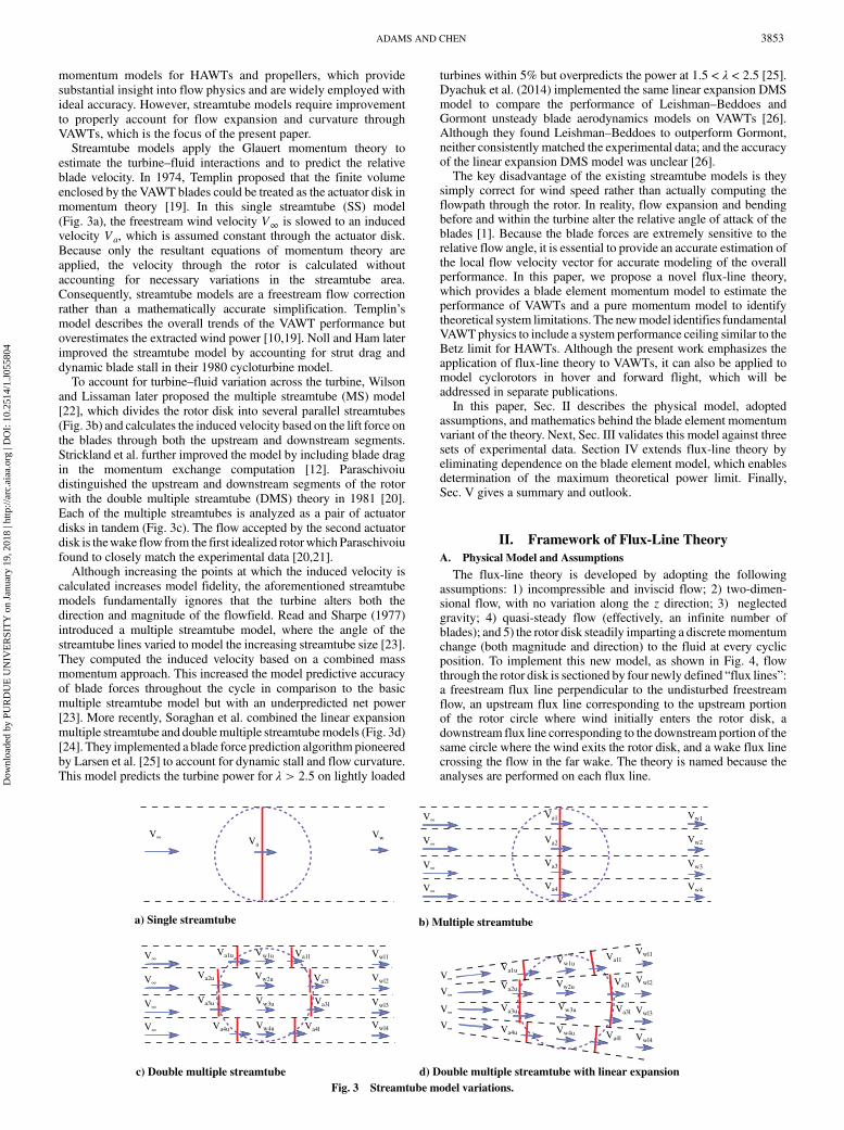
momentum models for HAWTs and propellers, which providesubstantial insight into flow physics and are widely employed withideal accuracy. However, streamtube models require improvementto properly account for flow expansion and curvature throughVAWTs, which is the focus of the present paper.Streamtube models apply the Glauert momentum theory to

estimate the turbine–fluid interactions and to predict the relativeblade velocity. In 1974, Templin proposed that the finite volumeenclosed by the VAWT blades could be treated as the actuator disk inmomentum theory [19]. In this single streamtube (SS) model(Fig. 3a), the freestream wind velocity V∞ is slowed to an inducedvelocity Va, which is assumed constant through the actuator disk.Because only the resultant equations of momentum theory areapplied, the velocity through the rotor is calculated withoutaccounting for necessary variations in the streamtube area.Consequently, streamtube models are a freestream flow correctionrather than a mathematically accurate simplification. Templin’smodel describes the overall trends of the VAWT performance butoverestimates the extracted wind power [10,19]. Noll and Ham laterimproved the streamtube model by accounting for strut drag anddynamic blade stall in their 1980 cycloturbine model.To account for turbine–fluid variation across the turbine, Wilson

and Lissaman later proposed the multiple streamtube (MS) model[22], which divides the rotor disk into several parallel streamtubes(Fig. 3b) and calculates the induced velocity based on the lift force onthe blades through both the upstream and downstream segments.Strickland et al. further improved the model by including blade dragin the momentum exchange computation [12]. Paraschivoiudistinguished the upstream and downstream segments of the rotorwith the double multiple streamtube (DMS) theory in 1981 [20].Each of the multiple streamtubes is analyzed as a pair of actuatordisks in tandem (Fig. 3c). The flow accepted by the second actuatordisk is thewake flow from the first idealized rotorwhich Paraschivoiufound to closely match the experimental data [20,21].Although increasing the points at which the induced velocity is

calculated increases model fidelity, the aforementioned streamtubemodels fundamentally ignores that the turbine alters both thedirection and magnitude of the flowfield. Read and Sharpe (1977)introduced a multiple streamtube model, where the angle of thestreamtube lines varied to model the increasing streamtube size [23].They computed the induced velocity based on a combined massmomentum approach. This increased the model predictive accuracyof blade forces throughout the cycle in comparison to the basicmultiple streamtube model but with an underpredicted net power[23]. More recently, Soraghan et al. combined the linear expansionmultiple streamtube and doublemultiple streamtubemodels (Fig. 3d)[24]. They implemented a blade force prediction algorithm pioneeredby Larsen et al. [25] to account for dynamic stall and flow curvature.This model predicts the turbine power for λ > 2.5 on lightly loaded

turbines within 5% but overpredicts the power at 1.5 < λ < 2.5 [25].Dyachuk et al. (2014) implemented the same linear expansion DMSmodel to compare the performance of Leishman–Beddoes andGormont unsteady blade aerodynamics models on VAWTs [26].Although they found Leishman–Beddoes to outperform Gormont,neither consistently matched the experimental data; and the accuracyof the linear expansion DMS model was unclear [26].The key disadvantage of the existing streamtube models is they

simply correct for wind speed rather than actually computing theflowpath through the rotor. In reality, flow expansion and bendingbefore and within the turbine alter the relative angle of attack of theblades [1]. Because the blade forces are extremely sensitive to therelative flow angle, it is essential to provide an accurate estimation ofthe local flow velocity vector for accurate modeling of the overallperformance. In this paper, we propose a novel flux-line theory,which provides a blade element momentum model to estimate theperformance of VAWTs and a pure momentum model to identifytheoretical system limitations. The newmodel identifies fundamentalVAWTphysics to include a system performance ceiling similar to theBetz limit for HAWTs. Although the present work emphasizes theapplication of flux-line theory to VAWTs, it can also be applied tomodel cyclorotors in hover and forward flight, which will beaddressed in separate publications.In this paper, Sec. II describes the physical model, adopted

assumptions, and mathematics behind the blade element momentumvariant of the theory. Next, Sec. III validates this model against threesets of experimental data. Section IV extends flux-line theory byeliminating dependence on the blade element model, which enablesdetermination of the maximum theoretical power limit. Finally,Sec. V gives a summary and outlook.

II. Framework of Flux-Line Theory

A. Physical Model and Assumptions

The flux-line theory is developed by adopting the followingassumptions: 1) incompressible and inviscid flow; 2) two-dimen-sional flow, with no variation along the z direction; 3) neglectedgravity; 4) quasi-steady flow (effectively, an infinite number ofblades); and 5) the rotor disk steadily imparting a discretemomentumchange (both magnitude and direction) to the fluid at every cyclicposition. To implement this new model, as shown in Fig. 4, flowthrough the rotor disk is sectioned by four newly defined “flux lines”:a freestream flux line perpendicular to the undisturbed freestreamflow, an upstream flux line corresponding to the upstream portionof the rotor circle where wind initially enters the rotor disk, adownstream flux line corresponding to the downstream portion of thesame circle where the wind exits the rotor disk, and a wake flux linecrossing the flow in the far wake. The theory is named because theanalyses are performed on each flux line.

a) Single streamtube b) Multiple streamtube

c) Double multiple streamtube

V∞ VaVw

V∞ Va4 Vw4

V∞ Va3 Vw3

V∞ Va2 Vw2

V∞ Va1 Vw1

V∞

V∞

V∞

V∞

Vwl4

Vwl3

Vwl2

Vwl1Va1u

Va2u

Va3u

Va4u

Vw1u

Vw2u

Vw3u

Vw4u

Va1l

Va2l

Va3l

Va4l

d) Double multiple streamtube with linear expansion

Vwl4

Vwl3

Vwl2

Vwl1

Va1u

Va2u

Va4u

Vw1u

Vw2u

Vw3u

Vw4u

Va1l

Va2l

Va3l

Va4l

V∞

V∞

V∞

V∞

Va3u

Fig. 3 Streamtube model variations.

ADAMS AND CHEN 3853

Dow

nloa

ded

by P

UR

DU

E U

NIV

ER

SIT

Y o

n Ja

nuar

y 19

, 201

8 | h

ttp://

arc.

aiaa

.org

| D

OI:

10.

2514

/1.J

0558

04

Each flux line can be labeled in a Cartesian system (by the three-

dimensional coordinates x–y–z) and a streamline system,

respectively. In the streamline system, a streamline index s is

assigned to each streamline within the domain, where all points on a

specific streamline are labeled by a consistent s �0 ≤ s ≤ 1�. The twomarginal streamlines, s � 0 and s � 1, are tangent to the rotor disk.Flow parameters (induced velocity, flow angle, forces, etc.) can be

described as either a function of the streamline position f�s� or theirCartesian location f�x; y�∕f�ϕ�. In the following analysis, subscripts∞, u, d, and w, denote parameters at the freestream flux line, the

upstream flux line, the downstream flux line, and the wake flux line,

respectively. The flux-line crossing angle γ is spanned by the

streamline and flux line at their intersection (Fig. 4). By this

definition, γ∞ � π∕2, 0 ≤ γu, γd ≤ π as s increases from zero to one,

and γw holds a constant value between zero and π.

B. Mathematics Describing Flow Physics

1. Conservation of Mass

A streamline s and its adjacent neighborhood

s −ds

2< s < s� ds

2

span a two-dimensional streamtube (inset of Fig. 4) with conserved

mass flux at every cross section, i.e.,

V∞A�s−�ds∕2�→s��ds∕2��∞ � Vu�s�A�s−�ds∕2�→s��ds∕2��

u

� Vd�s�A�s−�ds∕2�→s��ds∕2��d

� Vw�s�A�s−�ds∕2�→s��ds∕2��w (1)

where A denotes the effective cross-sectional area of the streamtube.

Considering unit depth along the z direction, the area is related to theflux-line coordinates of the two streamlines. Thus, from Eq. (1),

one has

V∞

�y∞

�s� ds

2

�− y∞

�s −

ds

2

��

� Vu�s�r�ϕu

�s� ds

2

�− ϕu

�s −

ds

2

��sin�γu�s��

� Vd�s�r�ϕd

�s� ds

2

�− ϕd

�s −

ds

2

��sin�γd�s��

� Vw�s��yw

�s� ds

2

�− yw

�s −

ds

2

��(2)

where y∞ and yw represent the y intercepts of the streamlines

with freestream and wake flux lines, respectively; and r is the

radius of the rotor disk. Applying a first-order Taylor’s expansion

yields

V∞dy∞ds

� Vu�s�rdϕu

dssin�γu�s�� � Vd�s�r

dϕd

dssin�γd�s��

� Vw�s�dywds

(3)

2. Conservation of Momentum

As the flow passes through the rotor disk, the interaction between

the flow and the blades induces a momentum change (or force),

extracted from or imparted to the fluid by rotating blades. This

interaction is modeled by assuming that only the force component

parallel to the streamline Fk contributes to this momentum (and

velocity) change, as will be detailed later. This permits direct

computation of the induced flow velocities from the blade forces.

Those velocities are combined with data of all the streamline forces

(including the perpendicular component F⊥) to compute the

directions atwhich the streamline s enters and exits the rotor disk, i.e.,angles γu�s� and γd�s�.The Glauert actuator disk theory [27], commonly applied to

propellers and HAWTs, is adopted in flux-line theory along each

streamline by assuming that an instantaneous static pressure change

occurs as flow passes through the actuator disk. At the entrance and

exit of the control volume, the pressure equalizes toP∞. The thrust or

drag applied on the actuator disk is equivalent to the change in

momentum:

T � _m�V∞ − Vw� � ρAVa�V∞ − Vw� (4)

where Va is the induced velocity across the actuator disk. T should

also balance the pressure drop across the actuator disk:

T � A�Pu − Pd� (5)

The Bernoulli equation relates the thrust and velocity of the far

wake:

T � 1

2ρA�V2

∞ − V2w� (6)

Combining Eqs. (4) and (6) gives

Va � 1

2�V∞ � Vw� (7)

The same analysis is applied to predict induced velocities at the

upstream and downstream flux lines. When the pressure is assumed

to restore to P∞ inside the rotor disk, similar to Eq. (7), one gets

Fig. 4 Schematic of flux-line model: system, geometry, and variables.

3854 ADAMS AND CHEN

Dow

nloa

ded

by P

UR

DU

E U

NIV

ER

SIT

Y o

n Ja

nuar

y 19

, 201

8 | h

ttp://

arc.

aiaa

.org

| D

OI:

10.

2514

/1.J

0558

04

Vu�s� �1

2

�V∞�s� � Vuwake �s�

�(8)

and

Vd�s� �1

2

�Vuwake�s� � Vw�s�

�(9)

where Vuwake is the flow velocity inside the rotor disk along thestreamline s. Vuwake can be determined by a control volume analysis,as shown in Fig. 5. As previously mentioned, Fk is assumed to onlychange thevelocitymagnitude; thus, the control volume is effectivelylinearly transformed (inset of Fig. 5), i.e.,

Fku � _m�V∞ − Vuwake

�(10)

The mass flow rate _m is the product of the density, velocity, andcross-sectional area. Thus,

Fku � ρVuAstreamtube

�V∞ − Vuwake

�(11)

Rearranging Eq. (11) yields

Vuwake � V∞ −Fku

ρAstreamtubeVu

(12)

The streamtube area is related to the flux-line area by

Astreamtube � Afluxline sin γ (13)

When considering an infinitesimal streamtube, it is convenient toconsider the force per unit area flux line: fku � Fku∕Afluxline.Substituting this expression into Eq. (12) yields

Vuwake � V∞ −fku

ρVu sin γu(14)

Substituting Eq. (14) into Eq. (8) eliminates the dependence on thewake velocity:

Vu � V∞ −fku

2ρVu sin γu(15)

Rearranging provides a quadratic equation:

V2u − VuV∞ � fku

2ρ sin γu� 0 (16)

where the only valid solution is

Vu�s� �V∞�s�

2�

�������������������������������������V2∞�s�4

−fku�s�2ρ sin γu

s(17)

The downstream flux-line induced velocity and wake velocity canbe similarly derived. By conservation of momentum,

_m�Vuwake − Vw

�� Fkd (18)

Rearranging gives the wake velocity

Vw � Vuwake −fkd

ρVd sin γd(19)

Substituting into Eq. (9) and rearranging gives

V2d − VdVuwake �

fkd2ρ sin γd

� 0 (20)

with the solution

Vd�s� �Vuwake �s�

2�

�����������������������������������������V2uwake �s�4

−fkd�s�2ρ sin γd

s(21)

Given the force [fku�s� and fkd�s�] and angular [γu�s� and γd�s�]distributions, Eqs. (17) and (21) predict the flux-line velocities atstreamline s without reference to the geometry of the system. Thispowerful result provides rapid calculation of rotor inflow. Once thevelocity is determined, the angle at which each streamline crosses theflux lines can be determined as explained in the following section.

3. Determining Flow Angles Across Each Flux line

To globally model the streamline bending through the rotor disk,we propose a two-parameter model to describe γu�s� and γd�s�.

4. Determining Flow Angles Across Each Fluxline: The Two Parameter

γ Model

The model functions for γu and γd must satisfy the followingproperties:1) γu�s � 0� � γd�s � 0� � 0.2) γu�s � 1� � γd�s � 1� � π.3) If the turbine does not produce any forces (no disturbance to the

incoming flow), the flow through rotor keeps uniform along the xdirection, leading to γu�s� � γd�s� � arccos�1–2s�.4) As the drag of the turbine increases, less flow proceeds through

the turbine. Increasing the drag causes the flow to resemble that of theflow around a circular cylinder. Consequently, at a high enough drag,the distributionmust converge toward a stagnation point distribution:

γu�s� � γd�s� �

8>>><>>>:0 when 0 ≤ s ≤

1

2

π when1

2< s ≤ 1

(22)

5) If the system is driven as a propeller with a large thrust, then theflow will curve into the circular rotor akin to flow in a bell-mouthengine inlet. Ultimately, a sufficiently large thrust should produce adistribution where the flow everywhere is perpendicular to theupstream flux line. Mathematically, γu�s� � π∕2 in this casefor 0 ≤ s ≤ 1.6) The distributions must be continuous and differentiable.We propose the following two-parameter (ϵ − η) models that meet

these requirements:

γu�s� � arctan

�2

������������������������sηu�1 − sηu�p

ϵu�1–2sηu��

(23)

and

γd�s� � arctan

�2

������������������������sηd�1 − sηd�p

ϵd�1–2sηd��

(24)

Streamtube

V∞ Vu

VwControl Volume

F||u

F⊥u

Fd

VdF||d

F⊥d

Vuwake

F||u

V∞

Vuwake

s

s+ds

Fu

Fig. 5 Streamtube, associated forces, and control volume forupper flux-line analysis.

ADAMS AND CHEN 3855

Dow

nloa

ded

by P

UR

DU

E U

NIV

ER

SIT

Y o

n Ja

nuar

y 19

, 201

8 | h

ttp://

arc.

aiaa

.org

| D

OI:

10.

2514

/1.J

0558

04

As shown in Fig. 6, γu�s� and γd�s� equate to arccos�1–2s� whenϵu � ϵd � 1 and ηu � ηd � 1. Figure 6 also compares various

predictions of γu�s� with different combinations of ϵ and η.Increasing ϵu (or ϵd) forms the distribution toward a stagnation point

distribution, whereas decreasing it nearer to zero molds the

distributions toward γu�s� � π∕2. Note that ϵu and ϵd are constrainedbetween zero and positive infinity. Changing the coefficients ηu(or ηd) alters the net skew of the wake. The mathematical limits of ηuare also between zero and positive infinity; however, only values near

one are physically sensible.The coefficients ϵu, ϵd, ηu, and ηd are determined by flow

momentum balances on the upstream and downstream flux lines

using a control volume analysis (Fig. 7) in the x direction

Z1

0

ρV∞dy∞ds

Vu cos θxu ds −Z

1

0

ρV2∞dy∞ds

ds

�Z

1

0

1

2ρ�V2

∞ − V2u� sinϕu

dϕu

dsr ds (25)

because

Pu�s� � P∞ � 1

2ρ�V2

∞ − V2u�s�� (26)

and

θxu�s� � ϕu�s� − γu�s� (27)

In the y direction,

Z1

0

ρV∞dy∞ds

Vu sin θxu ds �Z

1

0

1

2ρ�V2

∞ − V2u� cosϕu

dϕu

dsr ds

(28)

Equations (25) and (28) are numerically solved for ϵu and ηu.Similarly, from momentum balances on the downstream control

volume, in the x direction,

Z1

0

ρV∞dy∞ds

Vd cosθxd ds−Z

1

0

ρV∞dy∞ds

Vu cosθxu ds

�Z

1

0

fuxdϕu

dsrds�

Z1

0

Pu sinϕu

dϕu

dsrds−

Z1

0

Pd sinϕd

dϕd

dsrds

(29)

and, in the y direction,

Z1

0

ρV∞dy∞ds

Vd sinθxd ds−Z

1

0

ρV∞dy∞ds

Vu sinθxu ds

�Z

1

0

fuydϕu

dsrds−

Z1

0

Pd cosϕd

dϕd

dsrds−

Z1

0

Pu cosϕu

dϕu

dsrds

(30)

where

Pd�s� � P∞ � 1

2ρ�V2uwake − V2

d�s��

(31)

and

θxd�s� � −ϕd�s� � γd�s� (32)

Equations (29) and (30) are numerically solved for ϵd and ηd.

C. Transformation to Cartesian Domain

The conservation laws determine the velocity, angles, and

relative spacing of streamlines as functions of streamline index s. Toyield forces and power, these parameters must be transformed back

into the Cartesian domain. This transformation centers on ensuring

that the upstream and downstream flux lines form a complete rotor

disk, i.e.,

Z1

0

dϕu�s�ds

ds�Z

1

0

dϕd�s�ds

ds � 2π (33)

s

γ u/π

0 0.2 0.4 0.6 0.8 10

0.2

0.4

0.6

0.8

1arccos(1-2s)ε =1, η=1; ε =0.05, η=1; ε =10, η=1; ε =1, η=2;

Fig. 6 Comparison of two-parameter distribution with inverse cosinedistribution for various coefficients.

Fig. 7 Control volumes for upstream and downstream flux-line gamma distribution analyses.

3856 ADAMS AND CHEN

Dow

nloa

ded

by P

UR

DU

E U

NIV

ER

SIT

Y o

n Ja

nuar

y 19

, 201

8 | h

ttp://

arc.

aiaa

.org

| D

OI:

10.

2514

/1.J

0558

04

Combining the conservation of mass [Eq. (3)] with Eq. (33)yieldsZ

1

0

V∞

Vu�s� sin�γu�s��rdy∞ds

ds�Z

1

0

V∞

Vd�s� sin�γd�s��rdy∞ds

ds� 2π

(34)

Given the known force distributions from a blade elementanalysis, dy∞∕ds is the only unknown. Rearranging provides

1

2r

dy∞ds

� πR10 �V∞∕Vu�s�sin�γu�s���ds�

R10 �V∞∕Vd�s�sin�γd�s���ds

(35)

The parameter dy∞∕ds holds special significance because itidentifies the area of freestream flow that is processed by the rotor.Its nondimensional form is the freestream area ratio:

A∞

Aprojected

� 1

2r

dy∞ds

(36)

which is the ratio of the projected rotor area to the freestream flowarea that proceeds through the rotor. Avalue of one signifies that thefreestream area is equal to the projected area of the rotor, whereassmaller or larger values correspond to equivalently changing areas(Fig. 8). If all portions of the turbine extract energy from the flow,the freestream wind area that is processed will be smaller than theturbine projected area due to flow expansion. In the extreme case ofinfinite drag, no flow will proceed through the rotor and thefreestream area ratio will be zero. For cyclorotor operation, thefreestream area will be larger from flow contraction before the rotor.For a hovering cyclorotor, the freestream area and the freestreamarea ratio will be infinite:

A∞

Aprojected

� 1

2r

dy∞ds

8>>>><>>>>:

� 0 A∞ � 0 �Cycloturbine with in finite drag�< 1 A∞ < Aprojected �Cycloturbine�� 1 if A∞ � Aprojected �Zeroloading�> 1 A∞ > Aprojected �Cyclorotor�� ∞ A∞ � ∞ �Cyclorotor in hover�

(37)

Once dy∞∕ds is known,ϕu�s�,ϕd�s�, and yw�s� are determined by

integrating Eq. (3):

ϕu�s� �Z

s

0

dϕu�s�ds

ds� ϕu�s � 0�

�Z

s

0

V∞

Vu�s� sin�γu�s��rdy∞ds

ds� ϕu�s � 0� (38)

ϕd�s� �Z

s

0

dϕd�s�ds

ds� ϕd�s � 0�

�Z

s

0

V∞

Vd�s� sin�γu�s��rdy∞ds

ds� ϕd�s � 0� (39)

yw�s� �Z

s

0

dyw�s�ds

ds� yw�s � 0� (40)

D. Computation of Power and Forces

1. Blade Element Method

A blade element method is employed to determine fk�s� and

f⊥�s�. The relative flow experienced by the blade is determined by

the vector sum of the induced velocity and rotational velocity of the

turbine blade. The magnitudes of these resultant velocities, as shown

in Fig. 9, are

Vru ����������������������������������������������������������������������Ωr cos γu � Vu�2 � �Ωr sin γu�2

q(41)

and

Vrd ����������������������������������������������������������������������Ωr cos γd � Vd�2 � �Ωr sin γd�2

q(42)

The directions can be specified by the angles between the resultant

velocities and the streamline:

ζu � arctan

�Ωr sin γu

Ωr cos γu � Vu

�(43)

ζd � arctan

�Ωr sin γd

Ωr cos γd � Vd

�(44)

The angles ζu and ζd are also used to decompose the lift L and

drag D into the components parallel and normal to the streamline.

Given the blade pitch angle θu or θd, the angles of attack can be

determined:

αu � θu − γu � ζu (45)

and

αd � θd � γd − ζu (46)

Now, with the determined local velocity and angle of attack, the

lift and drag forces on the blade can be determined by interpolation

of experimental data (lift–drag characteristics), predictions of thin

airfoil theory, or other methods. Advanced double multiple

streamtube models used for VAWTs and cyclorotors model the

< 1 , CycloturbineA∞Aprojected

= 1 , Zero LoadingA∞Aprojected

> 1 , CyclorotorA∞Aprojected

Net Drag Net Thrust

Fig. 8 Expansion or contraction of flow through the rotor, described by the freestream area ratio.

ADAMS AND CHEN 3857

Dow

nloa

ded

by P

UR

DU

E U

NIV

ER

SIT

Y o

n Ja

nuar

y 19

, 201

8 | h

ttp://

arc.

aiaa

.org

| D

OI:

10.

2514

/1.J

0558

04

dynamic lift and poststall behavior [24,26,28–30]. In the present

analysis, the method by Rathi [29] is adjusted to account for

curvilinear flow [31] by combining the result from the thin airfoil

theory with a polynomial fit of poststall data by Critzos and Heyson

[32] to provide the aerodynamic coefficients at full 360 deg angles

of attack. To compute the lift and drag coefficients, the Oswald

efficiency factor e, the parasite drag coefficient CDo, the blade

aspect ratio, as well as the positive and negative stalling angles of

attack must be specified.Once the lift and drag forces are known, they may be related to the

forces on each streamline. A central assumption of flux-line analysis

is steady flow. However, the force of each blade on the flow from an

Eulerian perspective is unsteady for a finite number of blades, which

is considered by time averaging. The blade force is distributed over

the chord of the blade c, of which n blades only cover σ portion of therotor circumference:

F � Fblade

σ

c(47)

where solidity for the cycloturbines is as follows:

σ � nc

2πr(48)

The distributed lift and drag forces are thus both dependent on the

chord length. Because the aerodynamic moment

�m � σ

�1

2ρV2

rCmc

��

is due to the production of vorticity, its interaction with the flow

cannot be modeled with this quasi-one-dimensional theory. For this

reason, it is omitted from the analysis. If desired, it can be integrated

into the blade element model to correct its effect on the power. Then,

the forces parallel and perpendicular to the streamline for the

upstream and downstream flux lines are

fku�s� �1

2ρV2

ruσ�Cd�αu� cos ζu − Cl�αu� sin ζu� (49)

f⊥u�s� �1

2ρV2

ruσ�Cl�αu� cos ζu � Cd�αu� sin ζu� (50)

fkd�s� �1

2ρV2

rdσ�Cd�αd� cos ζd � Cl�αd� sin ζd� (51)

and

f⊥d�s� �1

2ρV2

rσ�Cl�αd� cos ζd − Cd�αd� sin�ζd� (52)

where Cl and Cd are the lift and drag coefficients, respectively.

2. Forces

Similarly, force components (per unit length in the z direction) onthe rotor can also be determined by integration over the upstream anddownstream flux lines:

Fux �Z

ϕu�s�1�

ϕu�s�0�

hfku�s� cos�ϕu�s� − γu�s��

− f⊥u�s� sin�ϕu�s� − γu�s��ir ⋅ dϕu (53)

Fdx �Z

ϕd�s�1�

ϕd�s�0�

hfkd�s� cos�ϕd�s� − γu�s��

− f⊥d�s� sin�ϕd�s� − γu�s��ir ⋅ dϕd; (54)

Fuy �Z

ϕu�s�1�

ϕu�s�0�

hfku�s� sin�ϕu�s� − γu�s��

� f⊥u�s� cos�ϕu�s� − γu�s��ir ⋅ dϕu (55)

Fdy �Z

ϕd�s�1�

ϕd�s�0�

hf⊥d�s� cos�ϕd�s� − γd�s��

− fkd�ϕd� sin�ϕd�s� − γu�s��ir ⋅ dϕd (56)

The resultant force applied on the rotor disk is then

F � �Fux � Fdx�i� �Fuy � Fdy�j (57)

where i and j are unit directional vectors along the x and y directions,respectively.

3. Aerodynamic Power

The aerodynamic power (per unit length in the z direction)collected by each streamtube is

dPu � −�fku cos γu � f⊥u sin γu�Ω ⋅ r dϕu (58)

at the upstream flux line and

dPd � �fku sin γd − f⊥d sin γd�Ω ⋅ r dϕd (59)

at the downstream flux line. The total power is determined byintegrating over the rotor disk:

P �Z

1

0

dPu

dϕu

dϕu

dsds�

Z1

0

dPd

dϕd

dϕd

dsds (60)

The power coefficient is then

CP � P

0.5ρV3∞Aprojected

� P

ρV3∞r

(61)

E. Flux-Line Theory: Summary

Collectively, the preceding elements predict turbine power andforces from specification of the turbine geometry, blade pitchingmotions (or angle of attack), and the operating conditions (windspeed, rotational speed, air density, etc.). Because the flux-line

Fig. 9 Angles pertinent to blade element analysis.

3858 ADAMS AND CHEN

Dow

nloa

ded

by P

UR

DU

E U

NIV

ER

SIT

Y o

n Ja

nuar

y 19

, 201

8 | h

ttp://

arc.

aiaa

.org

| D

OI:

10.

2514

/1.J

0558

04

description of the flow through the turbine requires knowledge ofthe forces (whereas the blade element model requires specificationof the flow conditions), the analysis is implemented in an iterativeapproach, as shown in Fig. 10. The basic procedures are as follows:1) The user must preprescribe the fluid properties (density, etc.),

blade specifications (airfoil model with lift–drag characteristics,chord length, span length, etc.), turbine geometries (rotor radius,etc.), and operating conditions (wind speed, rotation speed, etc.), aswell as an applied blade pitching motion [given θ�ϕ�].2) Initially, the fluid conditions passing the rotor disk are guessed

to be those of the freestream flow [i.e., the velocity distributions arethe freestreamvelocityVu�s� � Vd�s� � V∞] and the γ distributionsapproximate that of γu�s� � γd�s� � arccos�1–2s� by choosingϵu � ϵd � 1 and ηu � ηd � 1 in the two-parameter γ model.3) Determine ζ and α from Eqs. (43–46), as well as Vr from

Eqs. (41) and (42).4) Model the airfoil lift–drag coefficients and compute the force

components fku and f⊥u to each streamline s from Eqs. (49–52).5) The forces are used in the flux-line momentum model to

calculate the fluid velocity [Vu�s�, Vd�s�], position [ϕu�s�, ϕd�s�],and direction [γu�s�, γd�s�] through the rotor.

a) Determine the updated Vu�s� from Eq. (17) and Vd�s� fromEqs. (12) and (21).b) Determine the freestream area ratio from Eq. (35) and ϕ�s�

from Eqs. (38) and (39).6)With the aforementioned updated values, determine the updated

coefficients ϵ and η in the two-parameter model by solving integralequations (25) and (28–30). This gives updated expressions of γu�s�and γd�s�. This system of integral equations must be solved with aroot-finding technique or numerical optimization. The present studyimplements the constrained sequential nonlinear optimizationalgorithm in the MATLAB function “fmincon.”7) Repeat procedures 3 to 6 until convergence is achieved.

Currently, convergence is achieved when the sum of the differencesbetween the induced velocities between adjacent iterations is smallerthan a chosen threshold.8) The converged results are fed into Eqs. (53–56) to compute the

force F applied on the rotor disk.

9) The aerodynamic power P is computed from Eqs. (60).Similar to the aforementioned streamtube models, this newly

proposed flux-line theory features a minimal computation cost, butwith an improved accuracy by accounting more realistic flow physics(bending and expansion). It can be easily implemented by a desktopcomputer, with computation lasting from a few minutes to tens ofminutes. Thus, oncevalidated, it represents a promising design tool forquickly predicting the performances of different designmodifications.

III. Model Validation

For model validation, we compared the predictions of flux-linetheory with three sets of published experimental data fromcyclorotor tests, for which the details are summarized in Table 1.Vandenberghe and Dick measured power, rotational speed, andwind velocity on a cyclorotor [14,33] by using a cam-based pitchadjustment mechanism predicted to be optimal based on previoustheoretical and wind-tunnel investigations. Madsen and Lundgren[34] reported a similar experiment by applying a pitch scheme ofθ�ϕ� � 6.6 sinϕ� 3.1 (in degrees). Benedict et al. performed asmall-scale wind-tunnel experiment by varying the phase andamplitude of a near-sinusoidal pitching motion [1].Figure 11 compares the various model predictions with

measurements by Vandenberghe and Dick [33]. All models predictthe power coefficient well at low loading conditions (in this case, alsolow TSRs), where there is little flow bending and the momentumexchange is small. As the TSR increases, there is more momentumexchange and disparities emerge. The flux-line theory predicts thetrend of the power reduction at λ > 2.5, but it slightly underpredictsthe magnitude ofCp. The single streamtube model fails to predict thetrend at a higher TSR, and other models severely underpredict Cp.The predictions from the flux-line theory also agree well with

experiments by Madsen and Lundgren [34], as shown in Fig. 12.These experiments collected data over a longer period of timeand experienced different turbulent conditions, which led tothe scattered appearance of experimental data in Fig. 12 despite theimplementation of averaging [34]. The flux-line theory provides thebest estimate of the highest density of experimental data points.

Blade ElementTheory

Momentum Theory: Fluxline Theory

Guess: γu(s),γd(s) (εu=εd=1, ηu=ηd=1)

Blade Angle of Attack (α( )) orBlade Pitch (θ( ))

Forces

Updated γu(s),γd(s) Updated Vu(s),Vd(s)

Iteration Loop

Operating Conditions(λ, ρ, V∞)

Guess: Vu(s)=Vd(s)=V∞

-Power-Lift-Drag-Streamline Position

Updated u(s), d(s)

Converged?

YesNo

Fig. 10 Block diagram of flux-line execution in a blade element momentum theory.

Table 1 Experimental conditions

Category Vandenberghe and Dick [14,33] Madsen and Lundgren [34] Benedict et al. [1]

Radius r, m 1.825 1.4 0.127Span b, m 2.4 3.3 0.254Chord c, m 0.365 0.28 0.034Solidity σ 0.0955 0.095 0.169Chord-to-radius ratio c∕r 0.152 0.084 0.114Rotor aspect ratio b∕2r 0.66 1.18 1Blade airfoil NACA0012 NACA0015 NACA0015Number of blades n 3 3 4Pitching axis location, % c 25% Not available 25%Pitching scheme Second-order optimum Sinusoidal Near sinusoidalFreestream velocity V∞, m∕s Variable Variable 10Tip speed ratio λ range 1.5–3 1–3.7 0.2–1.1

Re � �cV∞��������������1� λ2

p∕ν� 300,000–800,000 150,000–450,000 23,000–35,000

Experimental conditions Open air Open air Open-jet wind tunnel

ADAMS AND CHEN 3859

Dow

nloa

ded

by P

UR

DU

E U

NIV

ER

SIT

Y o

n Ja

nuar

y 19

, 201

8 | h

ttp://

arc.

aiaa

.org

| D

OI:

10.

2514

/1.J

0558

04

Presumably, this suggests that it most accurately predicts the trueturbine efficiency in a controlled test with consistent atmosphericturbulence. At low TSRs, all of the theories give matched results, butthey slightly overpredict the experimental data. Likely, this is a resultof an improperly matched blade element model, because there isnearly uniform flow at low turbine loading conditions.The flux-line theory also accurately models the performance

under lower-Reynolds-number and low TSR conditions, which areidentical to the ones reported by Benedict et al. [1]. Figure 13compares the predictionswith 10 and 20 deg near-sinusoidal pitchingmotions on a small cycloturbine. The flux-line theory slightlyoverpredicts the power at all TSRs in both tests but provides a betterestimate than the other streamtube theories. Again, the discrepancybetween prediction and measurement is amplified with the increasedTSR and turbine loading. This accurate modeling is accomplished in

a negligible computational time on an ordinary desktop computer.Consequently, the model is tractable for implementation inoptimization algorithms, where many iterations are required.As a low-order model, the flux-line theory has unavoidable

limitations. First, it computes the wake velocity by assuming a totalpressure loss across the flux line and then a full expansion of thewakeflow to ambient pressure. This assumption is valid in the far wake ofthe turbine but is questionable within the rotor disk. Therefore, itlikely overestimates the flow expansion and underpredicts thedownstream induced velocity. In the case of a highly loaded rotorfront and lightly loaded rear, the model will underpredict the powercoefficient. In no case will the enforcement of flow expansion causean overprediction of the power coefficient. Second, a numericaliteration is required to combine the blade element portion of themodelwith themomentummethod for rapid results. To do so, the flux

Fig. 11 Blade pitch adjustment schemeadoptedbyVandenberghe andDick experimental cycloturbine (left) [14,33]; and comparison of predictions from

flux-line theory, DMS, MS, and SS models with measurement data (right). The experimental result represents the net power from the blades, whichexcludes the parasite power loss from the rotor structure. An identical steady blade element model fromRathi [29] was implemented with an adjustmentfor curvilinear flowviaMiglore et al. [31] for allmomentummodels. The followingparameterswere selected in themodel analysis: interior stalling angle ofattack of 25 deg, exterior stalling angle of attack of 15 deg, parasite drag coefficient of 0.022, andOswald efficiency factor of 0.85. Flow through the turbinewas discretized into 30 streamtubes.

Fig. 12 Madsen andLundgren [34] experimental cycloturbine blade pitch adjustment scheme (left); and comparison of flux-line theory, DMS,MS, DSS,

andSSmodelswith data (right). The experimental data aremathematically adjusted for net power from the gross aerodynamic power byMadsen et al. Anidentical steady blade element model from Rathi [29] was implemented, with adjustment for curvilinear flow via Migliore et al. [31] for all momentummodels. The following parameters were selected: interior stalling angle of attack of 25 deg, exterior stalling angle of attack of 15 deg, parasite dragcoefficient of 0.018, and Oswald efficiency factor of 0.85. Flow through the turbine was discretized into 30 streamtubes.

3860 ADAMS AND CHEN

Dow

nloa

ded

by P

UR

DU

E U

NIV

ER

SIT

Y o

n Ja

nuar

y 19

, 201

8 | h

ttp://

arc.

aiaa

.org

| D

OI:

10.

2514

/1.J

0558

04

lines must be discretized by the streamline index s. However, thiscreates nonsensible solutions at many turbine operating conditionsbecause the portion of the rotor circumference encompassed by thetwo near endpoints is greatly exaggerated. Near s � 0 and s � 1,the values of γu and γd approach zero. Consequently, the contributionof term

V∞

Vu�s� sin�γu�s��

becomes significant in the expressions for dy∞∕ds, dϕu∕ds, anddϕd∕ds. In principle, this is not a problem because the portion of the sdomain that they encompass is small. However, when the model isdiscretized, these large values are disproportionately represented. Inturn, the functions ϕu�s� and ϕd�s� may be erroneously predicted.This shortcoming can be mitigated by varying the spacing of thediscretization points, limiting the range of γu and γd to a valuesomewhat above zero and below π, or capping the value described of

V∞

Vu�s� sin�γu�s��

The second method is most easily implemented and chosen in thecurrent study.

IV. Flux-Line Pure Momentum Theory

The preceding blade element momentum implementation of theflux-line theory provides an effective cycloturbine design andevaluation tool. Moreover, when the dependence on the bladeelement model is eliminated, the flux-line theory provides generalinsights into cycloturbine flow physics. A key conclusion of this

analysis is the establishment of a performance limit akin to the

Betz limit prescribed for HAWTs. In this “pure” momentum

implementation of the flux-line theory, interference factors are

prescribed for the upstream and downstream flux lines that are similar

to the induction factor in the one-dimensional (1-D) actuator disk

model for HAWTs instead of detailed blade geometry and pitching

motions. The interference factors au and ad for the upstream and

downstream flux lines are introduced by

auV∞ � V∞ − Vu (62)

and

adVuwake � Vuwake − Vd (63)

Following a similar analysis as in the 1-D actuator disk model, one

has

2auV∞ � V∞ − Vuwake (64)

and

2adVuwake � Vuwake − Vw (65)

Rearranging yields

Vu � V∞�1 − au� (66)

Vuwake � V∞�1–2au� (67)

Fig. 13 Blade pitch motion adopted in experimental cycloturbine by Benedict et al. at the University of Maryland (UMD) for pitch amplitudes of 10 deg(left) and 20 deg (right), respectively (top) [1]. Comparison of predictions from flux-line theory, DMS, MS, DSS, and SS models with measurements(bottom). The symbols represent the measured net power from the blades, which excludes the parasite power loss from the rotor structure. An identical

steady blade element model from Rathi [29] was implemented, with adjustment for curvilinear flow via [31] for all momentum models. The followingparameters were selected: interior stalling angle of attack of 28 deg, exterior stalling angle of attack of 9 deg, parasite drag coefficient of 0.02, andOswaldefficiency factor of 0.85. Flow through the turbine was discretized into 30 streamtubes.

ADAMS AND CHEN 3861

Dow

nloa

ded

by P

UR

DU

E U

NIV

ER

SIT

Y o

n Ja

nuar

y 19

, 201

8 | h

ttp://

arc.

aiaa

.org

| D

OI:

10.

2514

/1.J

0558

04

Vd � Vuwake �1 − ad� � V∞�1–2au��1 − ad� (68)

Vw � Vuwake�1–2ad� � V∞�1–2au��1–2ad� (69)

These equations can be combined with the results of the

momentum theory analysis. Starting with the upstream flux line,

multiplying Eq. (14) by Vu yields

VuwakeVu � V∞Vu −fku

ρ sin γu(70)

Substituting in Eqs. (66) and (67) gives

V2∞�1 − au��1–2au� � V2

∞�1 − au� −fku

ρ sin γu(71)

which simplifies to

au�1 − au� �fku

2ρV2∞ sin γu

(72)

or, alternatively,

fku � 2ρV2∞au�1 − au� sin γu (73)

The same analysis can be performed on the downstream flux line,

yielding [starting from Eq. (19)]

fkd � 2ρ sin γdV2∞�1–2au�2�1 − ad�ad (74)

For a turbine blade operated under normal conditions, the lift force

is significantly greater than the drag force, which is thus neglected in

the following analysis to estimate the optimal power. This

simplification allows the force parallel to each streamline (as shown

in Fig. 9 whenD � 0) to be related to the force perpendicular to eachstreamline:

fku− sin ζu

� f⊥ucos ζu

(75)

Similarly,

fkdsin ζd

� f⊥dcos ζd

(76)

Rearranging gives the perpendicular streamline forces as functions

of the interference factors

f⊥u � −fkutan ζu

� −2ρV2∞ sin γuau�1 − au�

tan ζu(77)

and

f⊥d � fkdtan ζd

� 2ρV2∞ sin γd�1–2au�2ad�1 − ad�

tan ζd(78)

Note that

tan ζu � Ωr sin γuΩr cos γu � Vu

� λ sin γuλ cos γu � �1 − au�

(79)

Now, the power can bewritten exclusively in terms of the tip speed

ratio, turbine geometry, and the upstream and downstream

interference factors. Note that these interference factors are functions

of the flux-line coordinate s, i.e., au�s� and ad�s�. The differentialpower is

dPu � Vufkurdϕu � 2ρV3∞ sin γuau�1 − au�2rdϕu (80)

and

dPd � Vdfkdrdϕd � 2ρV3∞ sin γd�1–2au�3ad�1 − ad�2rdϕd

(81)

Rewriting the transformation equations produces a term for the

flux-line spatial derivatives in terms of the interference factors:

dy∞ds

� 2rπR10 �ds∕�1 − au� sin�γu�s��� �

R10 �ds∕�1–2au��1 − ad� sin�γd�s���

(82)

From Eq. (60), the power is

P �Z

1

0

dPu

dϕu

dϕu

dsds�

Z1

0

dPd

dϕd

dϕd

dsds (83)

which is expanded to

P � 2ρV3∞dy∞ds

�Z1

0

au�1 − au� ds�Z

1

0

�1–2au�2ad�1 − ad� ds�

(84)

The coefficient of power is calculated directly from the total power:

Cp � 4π

R10 au�s��1 − au�s�� ds�

R10 �1–2au�s��2ad�s��1 − ad�s�� dsR

10 �ds∕�1 − au�s�� sin�γu�s��� �

R10 �ds∕�1–2au�s���1 − ad�s�� sin�γd�s���

(85)

Because the velocity through the rotor is initially specified,iteration is not required. The angles γu�s� and γd�s� must be

modeled. The two-parameter model previously described is used.Consequently, the flux-line pure momentum theory predicts theperformance of a cycloturbine based only on the specification of the

interference functions.

A. Establishment of a Theoretical Performance Limit

The flux-line pure momentum theory places a theoreticalperformance limit for VAWTs similar to the Betz limit for HAWTs.This limit is obtained by optimizing the distributions of au�s� andad�s� to maximize the coefficient of power in Eq. (85). Thedistributions γu�s� and γd�s�must bemodeled and have a strong effect

on the maximum power coefficient. The following section provides anumerical optimization routine employing the two-parameter modeldescribed previously. Alternatively, the interference distributions can

be fixed as constants in a simplified analytical analysis.

3862 ADAMS AND CHEN

Dow

nloa

ded

by P

UR

DU

E U

NIV

ER

SIT

Y o

n Ja

nuar

y 19

, 201

8 | h

ttp://

arc.

aiaa

.org

| D

OI:

10.

2514

/1.J

0558

04

1. Numerical Optimization for Determination of Performance Limit

For numerical optimization, the efficient internal point nonlinearsequential constrained optimization technique is implemented via theMATLAB function fmincon, which requires a finite number ofdesign variables rather than optimization functions. Consequently,the distributions of interference factors au�s� and ad�s� areapproximated by a series of design variables xi, i � 1: l, withan applied cubic polynomial interpolation along each function.A convergence study determines that 11 points (l � 11) are requiredto adequately define the interference functions for a coefficient ofpower within 0.01.The generated functions are evaluated by constraint functions.

Also, au�s� and ad�s� are constrained by the maximum lift that theblades can generate:

L ≤1

2ρV2

rσCLmax(86)

A range of rotor solidities and a maximum blade lift coefficient of2.5 are selected. To enforce the determination of smooth andreasonable functions, the derivative�

dauds

;dadds

�

and the second derivative of the interference functions

�d2auds2

;d2adds2

�

are constrained to reasonable ranges: dads < 4

1

rad

and d2ads2

< 11

rad2

Furthermore, to ensure a positive far-wake velocity, the followingconstraint function is applied:

�1–2au�2�1–2ad� > 0 (87)

If the power is maximized under only these constraints, thesolution is unbounded and there is no limit to the maximum turbinepower. In those unbounded solutions, the upstream flux-lineinterference function is less than zero and the downstreamdistribution greater than zero. This corresponds to a dual propeller-turbine operating mode. Theoretically, the upstream portion of theturbine puts power into the flow, which accelerates and contracts alarger freestream area of wind than the actual projected turbine area(au < 0, �A∞∕Aprojected� > 1). Then, the downstream portion of theturbine retards (ad > 0) and isentropically extracts the greater totalwind energy. In this model, the freestream area ratio is greater thanone, and the wake velocity is less than the freestream velocity, asshown in Fig. 14. Mounting higher-order system inefficiencies maymake this combined propeller-turbine operating mode difficult orimpossible to realize. However, the idea warrants future in-depthevaluation.To place a more realistic limit on system power, the interference

functions were further constrained to only positive values less than0.5, i.e., 0 ≤ au�s� ≤ 0.5 and 0 ≤ ad�s� ≤ 0.5. This forces turbine-

only operation, where all portions of the turbine are only permitted todecelerate the flow. The sequential constrained optimization routineidentified themost efficient interference distributions at a range of tipspeed ratios, as depicted in Fig. 15. The performance limit for aVAWT is found by computingCp for these interference distributionsover a range of tip speed ratios. This dependence is compared withother performance limits in Fig. 16. The flux-line theory suggeststhat, to yield the optimum power, the upstream flux line should notdecelerate the flow (working at a zero loading status) and thedownstream flux line should decelerate the flow to just under 2∕3(i.e., ad ≳ 1∕3) of the freestream value atmoderate TSRs. Blade pitchmotions should then be designed to produce the interference factorsin Fig. 15 for optimum performance. The mechanism for this powerextraction is a greater effective area over the downstream portion ofthe turbine, which is explained in Sec. IV.A.3.These interference distributions produce a maximum cycloturbine

coefficient of power that increases from zero to a limit of 0.597 withincreasing TSR. This represents only a marginal improvement fromthe 1-D Betz limit of 0.593 [35]. The rate of performance increasesteepens with solidity because those rotors can exert greaterdeceleration forces on the fluid for the same available blade relativevelocity. In theory, the cycloturbine maximum power coefficientexceeds the rotating HAWT limit [27] at TSRs near two to three.Historically, cycloturbines have been designed with low solidity foroperation at high TSRs. However, they were often constrained toTSRs less than three to limit rotational speed for structural reasons orachieved low performance at high TSRs due to support structure draglosses. The performance of turbines can be improved by using a largerrotor solidity and maintaining only moderate TSRs. However,increasing the solidity will also magnify blade parasite drag from theadditional area and induced drag from reduced blade aspect ratio.Consequently, therewill be a design solidity and rotational speed thatprovides the best power that will depend on the exact aerodynamiccharacteristics of the geometry. This tradeoff deserves additionalconsideration in a future study.It must be cautioned that this flux-line performance limit is

sensitive to the model selected for γu�s� and γd�s�. Other modelswill provide different values. The dependence of the maximumcoefficient of power and the optimum interference distributions onthe inflow model is explored next.

2. Simplified Analytical Analysis of Maximum Performance

An alternative optimization technique is to select interferencefunctions for au�s� and ad�s� that are dependent only on a variableinterference constant. The simplest choice is to suppose that thesedistributions are constants, i.e., au�s� � Au and ad�s� � Ad.Substituting into Eq. (85) yields

Cp � 4πAu�1 − Au� � �1–2Au�2Ad�1 − Ad�

�1∕1 − Au�R10 �ds∕ sin γu� � �1∕�1–2Au��1 − Ad��

R10 �ds∕ sin γd�

(88)

DragThrust

au<0 ad>0

> 1 A ∞A projected

Fig. 14 Isentropic cycloturbine with infinite blades that could contractan area of freestream flow greater than the projected area of the rotorthrough utilization of cyclorotor pitching kinematics in the front half ofthe turbine. The flow could then be expanded in the rear half for acoefficient of power greater than one.

ADAMS AND CHEN 3863

Dow

nloa

ded

by P

UR

DU

E U

NIV

ER

SIT

Y o

n Ja

nuar

y 19

, 201

8 | h

ttp://

arc.

aiaa

.org

| D

OI:

10.

2514

/1.J

0558

04

If the ratio of integrals is defined as a variable κ

κ �R10 �ds∕ sin γd�R10 �ds∕ sin γu�

(89)

then the coefficient of power function simplifies to

Cp � 4πR10 �ds∕ sin γu�

Au�1 − Au� � �1–2Au�2Ad�1 − Ad��1∕�1 − Au�� � �κ∕�1–2Au��1 − Ad��

(90)

This expression is convenient to evaluate: if

Z1

0

ds

sin γu

is taken as a constant for small variations in the interference

distribution constants, the partial derivatives depend only on the ratio

of the γ distribution integrals but not their explicit value. Figure 17

plots Eq. (90) for

Z1

0

ds

sin γu� π

2

and κ � 1. In these plots, there is no clear local maximum due to the

presence of combined propeller-turbine operating modes (denoted

in the right contour plot) that theoretically have an unbounded

coefficient of power. Again, the feasibility of this operating regime

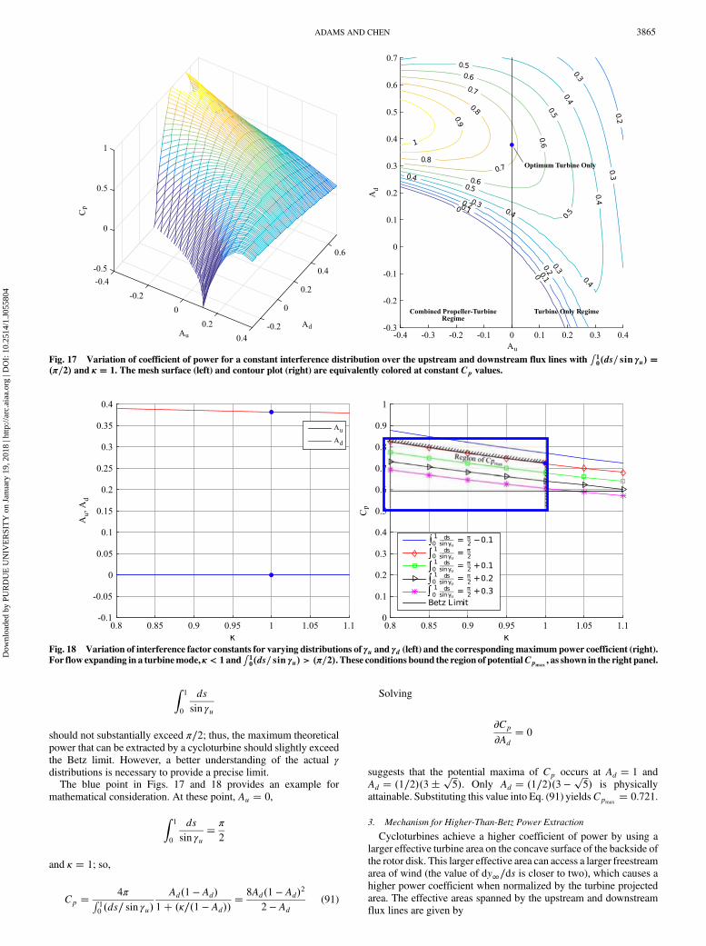
requires further investigation.Determining the root of the partial derivative �∂Cp∕∂Ad� � 0 at

Au � 0 provides the optimum interference coefficient values for the

turbine-only operatingmode. These values are plotted in Fig. 18. The

interference constants are nearly constant over a wide range of κ(Au � 0 and 0.38 < Ad < 0.39). Thus, the optimum interference

constants are quasi independent of the actual γ distributions. This

eliminates the requirement to model those distributions to obtain an

efficient distribution. However, the maximum Cp still requires

computation of both γ distributions. The potential values of this areplotted on the right side of Fig. 18. For the expansion of flow in a

turbine, κ < 1. For the unloaded turbine, we have γ � arccos�1–2s�;thus,

Z1

0

ds

sin γu� π

2

and for a loaded cycloturbine, we have

Z1

0

ds

sin γu>

π

2

Consequently, this narrows themaximumCp region to that shown on

the right of Fig. 18. Because the flow expansion should not be

dramatic,

Fig. 15 Optimum distributions of interference factors: au�s� (left) and ad�s� (right) for a rotor solidity of 0.2.

Fig. 16 Comparison of the flux-line theory performance limit with other wind turbine performance limits for varying rotor solidity. The rotating wakeHAWT limit and Betz 1-D limit are not applicable to VAWTs and are presented for comparison only.

3864 ADAMS AND CHEN

Dow

nloa

ded

by P

UR

DU

E U

NIV

ER

SIT

Y o

n Ja

nuar

y 19

, 201

8 | h

ttp://

arc.

aiaa

.org

| D

OI:

10.

2514

/1.J

0558

04

Z1

0

ds

sin γu

should not substantially exceed π∕2; thus, the maximum theoretical

power that can be extracted by a cycloturbine should slightly exceed

the Betz limit. However, a better understanding of the actual γdistributions is necessary to provide a precise limit.The blue point in Figs. 17 and 18 provides an example for

mathematical consideration. At these point, Au � 0,

Z1

0

ds

sin γu� π

2

and κ � 1; so,

Cp � 4πR10 �ds∕ sin γu�

Ad�1 − Ad�1� �κ∕�1 − Ad��

� 8Ad�1 − Ad�22 − Ad

(91)

Solving

∂Cp

∂Ad

� 0

suggests that the potential maxima of Cp occurs at Ad � 1 and

Ad � �1∕2��3� ���5

p �. Only Ad � �1∕2��3 − ���5

p � is physically

attainable. Substituting this value into Eq. (91) yieldsCpmax� 0.721.

3. Mechanism for Higher-Than-Betz Power Extraction

Cycloturbines achieve a higher coefficient of power by using a

larger effective turbine area on the concave surface of the backside of

the rotor disk. This larger effective area can access a larger freestream

area of wind (the value of dy∞∕ds is closer to two), which causes a

higher power coefficient when normalized by the turbine projected

area. The effective areas spanned by the upstream and downstream

flux lines are given by

Fig. 18 Variation of interference factor constants for varying distributions of γu and γd (left) and the correspondingmaximum power coefficient (right).For flow expanding in a turbinemode, κ < 1 and ∫ 1

0�ds∕ sin γu� > �π∕2�. These conditions bound the region of potentialCpmax, as shown in the right panel.

Fig. 17 Variation of coefficient of power for a constant interference distribution over the upstream and downstream flux lines with ∫ 10�ds∕ sin γu� �

�π∕2� and κ � 1. The mesh surface (left) and contour plot (right) are equivalently colored at constant Cp values.

ADAMS AND CHEN 3865

Dow

nloa

ded

by P

UR

DU

E U

NIV

ER

SIT

Y o

n Ja

nuar

y 19

, 201

8 | h

ttp://

arc.

aiaa

.org

| D

OI:

10.

2514

/1.J

0558

04

Aeu �Z

1

0

sin�γu�dϕu

dsr ds �

Z1

0

1

�1 − au�dy∞ds

ds (92)

and

Aed �Z

1

0

sin�γd�dϕd

dsr ds �

Z1

0

1

�1–2au��1 − ad�dy∞ds

ds (93)

For any turbine-only interference, distribution on the downstreamflux line will always have a greater effective area than the upstreamflux line. Because flow is expanding through the downstream fluxline, the downstream effective area is also greater than the equivalentprojected area of the turbine, i.e.,

Aed ≥ Aprojected ≥ Aeu (94)

This mechanism is markedly different than that suggested byNewman [36], who used a modified streamtube method to derivea similar performance limit for VAWTs. That mathematicalderivation resembled a 1-D double actuator disk theory, whereslightly higher theoretical performance (Cpmax

� 16∕25) wasachieved by incrementally expanding the flow across two actuatordisks. Figure 16 presents Newman’s theoretical limit, which suggeststhat VAWTs only marginally exceed the Betz limit at extremely highTSRs [36].Because streamtubemodels do notmodel flowexpansion,the effective areas of the upstream and downstream portions of therotor are equal. In flux-line theory, increasing the interference factoron the upstream portion of the rotor au disproportionately reduces thearea of the freestreamwind processed by the rotor as compared to thedownstream interference factorad, as shown inEq. (82). This reducesthe advantage of using both the upstream and downstreamportions ofthe rotor for flow deceleration.

V. Conclusions

A novel low-order blade element momentummodel for predictingthe performance of cycloturbines, named flux-line theory, isdeveloped. It accounts for the bending and expansion/contraction ofthe flow by computing fluid characteristics along each streamlinewithout a predescribed spatial location. A transformation determinesthe Cartesian location of streamlines, and additional calculationsdetermine the power and forces produced. Predictions of flux-linetheory are validated against three sets of experimental data measuredat a range of Reynolds numbers and pitch motions. The newmodel isextended to flux-line pure momentum theory, which eliminatesdependence on the blade elementmodel, to gain insight into optimumblade–fluid interaction. An analysis with this theory identifies themaximum theoretical turbine performance and optimum flowconditions, which is an essential precursor for determining optimalblade pitch kinematics. The following conclusions are drawn fromthis study:1) The flux-line theory accurately models the coefficient of power

for cycloturbines at a range of TSRs (0 ≤ λ ≤ 3) and Reynoldsnumbers by modeling the flow expansion and bending effects. Itpredicts the performance more accurately than single, double, singlemultiple, and double multiple streamtube models implementing thesame simple blade element model. The flux-line theory is a useful toolfor designing preliminary pitchingmotions and cycloturbine geometry.2) The flux-line puremomentum theory eliminates the dependence

on a blade element model by adopting distributions of interferencefactors on the upstream and downstream flux lines (where flowcrosses the rotor blade path). This simplified variation of flux-linetheory is useful for understanding the aerodynamic characteristics ofthe cycloturbine system. It suggests that cycloturbines can producethe most power when they are operated in a dual propeller-turbinemode. In this mode, the upstream portion of the turbine acts as apropeller (with energy consumption) and contracts a larger area of thefreestream wind; the downstream portion harvests wind energywhere thewind is expanded. Flux-line theory provides no theoreticallimit to the maximum turbine power production under thesecircumstances. However, feasible implementation of this concept,

where unsteady blade interaction and blade drag will be significant,seems unlikely and requires further investigation.3) If the cycloturbine is operated in a turbine-only mode, the flux-

line pure momentum theory can provide a theoretical vertical-axiswind turbines performance limit through optimization ofinterference factor distributions au�s� and ad�s�. The limit isdependent on the choice of the model used to describe the angle atwhich the flow crosses the upstream and downstream flux lines.Using a two-parameter model that matches experimental data, thelimit is numerically determined as 0.597. A simplified analyticalapproach determines a range of maximum value of the coefficient ofpower that is likely greater than 16∕27 but less than 0.8.4) To harvest the maximum power, the theory suggests that the

upstream blades should extract no energy from the flow (operate atzero blade lift coefficient), whereas the downstreamblades reduce thevelocity by slightly more than one-third of the freestream value. Thisbest power interference function is quasi independent of the choicesof the flow angle (γu and γd) distribution model.5) Flux-line pure momentum theory suggests that cycloturbines

have a higher theoretical power coefficient than horizontal-axis windturbines because they have a larger effective area than the projectedequivalent area. This contrasts a previous theory by Newman [36]that predicted that cycloturbines could achieve higher performanceby splitting the expansion of the flow across the upstream anddownstream portions of the rotor.

Acknowledgments

We thank theU.S.Department ofDefense for theNationalDefenseScience and Engineering Fellowship for enabling this work.Moreover, we thank Casey Fagley, Thomas McLaughlin, AngelaSuplisson, and Neal Barlow at the U.S. Air Force Academy forintroducing the problem of blade pitch kinematics on cyclorotors.

References

[1] Benedict, M., Lakshminarayan, V., Pino, J., and Chopra, I.,“Fundamental Understanding of the Physics of a Small-Scale VerticalAxisWind TurbinewithDynamic Blade Pitching: An Experimental andComputational Approach,” AIAA/ASME/ASCE/AHS/ASC Structures,

Structural Dynamics, and Materials Conference, AIAA Paper 2013-1553, April 2013.

[2] Dabiri, J., “Potential Order-of-Magnitude Enhancement of Wind FarmPower Density via Counter-Rotating Vertical-Axis Wind Farm TurbineArrays,” Journal of Renewable and Sustainable Energy, Vol. 3,July 2011, Paper 043104.

[3] Kirke, B. K., “Evaluation of Self-Starting Vertical Axis Wind Turbinesfor Stand-Alone Applications,” Ph.D. Thesis, School of Engineering,Griffith Univ., Gold Coast Campus, Southport, QLD, Australia,April 1998.

[4] Borg, M., Shires, A., and Collu, M., “Offshore Floating Vertical AxisWind Turbines, Dynamic Mode Model State of the Art. Part I:Aerodynamics,” Renewable and Sustainable Energy Reviews, Vol. 39,Aug. 2014, pp. 1214–1225.doi:10.1016/j.rser.2014.07.096

[5] Borg, M., Collu, M., and Kolios, A., “Offshore Floating Vertical AxisWind Turbines, Dynamics Modelling State of the Art. Part II: MooringLine and Structural Dynamics,” Renewable and Sustainable Energy

Reviews, Vol. 39, July 2014, pp. 1226–1234.doi:10.1016/j.rser.2014.07.122

[6] Sasson, B., and Greenblatt, D., “Effect of Leading-Edge Slot Blowingon a Vertical Axis Wind Turbine,” AIAA Journal, Vol. 49, No. 9, 2011,pp. 1932–1942.doi:10.2514/1.J050851

[7] Greenblatt, D., Ben-Harav, A., and Mueller-Wahl, H., “Dynamic StallControl on a Vertical-Axis Wind Turbine Using Plasma Actuators,”AIAA Journal, Vol. 52, No. 2, 2014, pp. 456–462.doi:10.2514/1.J052776

[8] Tescione, G., Ferreira, C., andVanBussel, G., “Analysis of a Free VortexWakeModel for the Studyof theRotor andNearWake Flowof aVerticalAxis Wind Turbine,” Renewable Energy, Vol. 87, Nov. 2016, pp. 552–563.doi:10.1016/j.renene.2015.10.002

[9] Shi, L., Riziotis, V., Voutsinas, S., and Wang, J., “A Consistent VortexModel for the Aerodynamic Analysis of Vertical Axis Wind Turbines,”

3866 ADAMS AND CHEN

Dow

nloa

ded

by P

UR

DU

E U

NIV

ER

SIT

Y o

n Ja

nuar

y 19

, 201

8 | h

ttp://

arc.

aiaa

.org

| D

OI:

10.

2514

/1.J

0558

04

Journal of Wind Engineering and Industrial Aerodynamics, Vol. 135,Dec. 2014, pp. 57–69.

[10] Islam, M., Ting, D., and Fartaj, A., “AerodynamicModels for Darrieus-Type Straight-Bladed Vertical Axis Wind Turbines,” Journal of

Renewable and Sustainable Energy, Vol. 12, No. 4, May 2008,pp. 1087–1109.doi:10.1016/j.rser.2006.10.023; also Noll, R. B., Ham, N. D., andPeraire, J., “Analytical Evaluation of theAerodynamic Performance of aHigh-Reliability Vertical-Axis Wind Turbine,” Proceedings of AWEA

National Conference, 1980.[11] Anderson, J., Brulle, R., Birchfield, E., and Duwe, W., “McDonnell

40 KwGiromill Wind System, Phase I: Design and Analysis, Volume I:Executive Summary,”McDonnell Aircraft Company TR RFP-3032/1,St. Louis, MO, 1979.

[12] Strickland, J., Webster, B., and Nguyen, T., “A Vortex Model of theDarrieus Turbine: An Analytical and Experimental Study,” Journal ofFluids Engineering, Vol. 101, No. 4, Dec. 1979, pp. 500–505.doi:10.1115/1.3449018

[13] Schatzle, P., Klimas, P., and Spahr, H., “Aerodynamic InterferenceBetween Two Darrieus Wind Turbines,” Sandia National Labs. TR,SAND81-0896, Albuquerque, NM, April 1981.

[14] Vandenberghe,D., andDick,E., “OptimumPitchControl forVerticalAxisWind Turbines,”Wind Engineering, Vol. 11, No. 5, 1987, pp. 237–247.

[15] Chowdhury, A., Akimoto, H., and Hara, Y., “Comparative CFDAnalysis of Vertical Axis Wind Turbine in Upright and TiltedConfiguration,” Renewable Energy, Vol. 85, July 2015, pp. 327–337.

[16] Li, C., Zhu, S., Xu, Y., and Xiao, Y., “2.5D Larger Eddy Simulation ofVertical Axis Wind Turbine in Consideration of High Angle of AttackFlow,” Journal of Renewable Energy, Vol. 51, Oct. 2013, pp. 317–330.doi:10.1016/j.renene.2012.09.011

[17] Howell, R., Qin, N., Edwards, J., and Durrani, N., “Wind Tunnel andNumerical Study of a Small Vertical Axis Wind Turbine,” Journal of

Renewable Energy, Vol. 35, No. 2, 2010, pp. 412–422.doi:10.1016/j.renene.2009.07.025

[18] Zuijlen, C. F. V., Bijl, H., Bussel, G. V., and Kuik, G. V., “SimulatingDynamic Stall in a Two-Dimensional Vertical-Axis Wind Turbine:Verification and Validation with Particle Image Velocimetry Data,”Wind Energy, Vol. 13, No. 1, May 2010, pp. 1–17.doi:10.1002/we.v13:1

[19] Templin, R., “Aerodynamic Performance Theory for the NRC Certical-AxisWind Turbine,”National ResearchCouncil Lab. TR LTF-LA-190,Ottawa, Ontario, June 1974.

[20] Paraschivoiu, I., “Aerodynamic Loads and Performance of the DarrieusRotor,” Journal of Energy, Vol. 6, No. 2, 1982.

[21] Paraschivoiu, I., and Delclaux, F., “Double Multiple Streamtube Modelwith Recent Improvements,” Journal of Energy, Vol. 7, No. 3, May–June 1983.

[22] Wilson, R., and Lissaman, P., “Applied Aerodynamics of Wind PowerMachines,” Oregon State Univ. Tech. Rept. GI-418340, Corvallis OR,July 1974.

[23] Read, S., and Sharpe, D., “An ExtendedMultiple StreamtubeModel forDarrieus Wind Turbines,” 2nd DOE/NASA Wind Turbines Dynamics

Workshop, NASA Paper CP-2186, Cleveland, OH, Feb. 1981,pp. 19–25.

[24] Soraghan, C., Leithead, W., Yue, H., and Feuchtwang, J., “DoubleMultiple Streamtube Model for Variable Pitch Vertical Axis WindTurbines,” AIAA Applied Aerodynamics Conference, AIAA Paper2013-2802, June 2013.

[25] Larsen, J., Nielsen, S., and Krenk, S., “Dynamic Stall Model for WindTurbine Airfoils,” Journal of Fluids and Structures, Vol. 23, 2007,pp. 959–982.

[26] Dyachuk, E.,Goude,A., andBernhoff,H., “DynamicStallModeling forthe Conditions of Vertical AxisWind Turbines,” AIAA Journal, Vol. 52,No. 1, Jan. 2014, pp. 72–81.doi:10.2514/1.J052633

[27] Wilson, R., Wind Turbine Technology, ASME Press, Fairfield, NJ,2009, pp. 281–350.

[28] Benedict, M., “Fundamental Understanding of the Cycloidal-RotorConcept for Micro Air Vehicle Applications,” Ph.D. Thesis, Univ. ofMaryland, College Park, MD, 2010.

[29] Rathi, D., “Performance Prediction and Dynamic Model Analysis ofVertical Axis Wind Turbine Blades with Aerodynamically VariedBlade Pitch,” M.S. Thesis, North Carolina State Univ., Raleigh, NC,2012.

[30] Asher, I., Drela, M., and Peraire, J., “A Low Order Model for VerticalAxis Wind Turbines,” AIAA Applied Aerodynamics Conference, AIAAPaper 2010-4401, June–July 2010.

[31] Migliore, P., Wolfe, W., and Fanucci, J., “Flow Curvature Effects onDarrieus Turbine Blade Aerodynamics,” Journal of Energy, Vol. 4,No. 2, 1980, pp. 49–55.doi:10.2514/3.62459

[32] Critzos, C., and Heyson, H., “Aerodynamic Characteristics of NACA0012 Airfoil Section at Angles of Attack from 0 to 180,” NACA TR3361, 1955.

[33] Vandenberghe, D., and Dick, E., “A Theoretical and ExperimentalInvestigation into the Straight Bladed Vertical Axis Wind Turbine withSecond Order Harmonic Pitch Control,” Wind Engineering, Vol. 10,No. 3, 1986, pp. 122–138.

[34] Madsen, H., and Lundgren, K., “The Voith-Schneider Wind Turbine,”Inst. of Industrial Constructions and Energy Technology, Aslborg Univ.Centre Tech. Rept. NP-2900722, Denmark, 1980.

[35] Leishman, G., Principles of Helicopter Aerodynamics, CambridgeUniv. Press, New York, 2006, pp. 730–731.

[36] Newman, B., “Actuator-Disc Theory for Vertical Axis Wind Turbines,”Journal of Wind Engineering and Industrial Aerodynamics, Vol. 15,Nos. 1–3, 1983, pp. 347–355.doi:10.1016/0167-6105(83)90204-0

M. SmithAssociate Editor

ADAMS AND CHEN 3867

Dow

nloa

ded

by P

UR

DU

E U

NIV

ER

SIT

Y o

n Ja

nuar

y 19

, 201

8 | h

ttp://

arc.

aiaa

.org

| D

OI:

10.

2514

/1.J

0558

04