Fluid-StructureInteractionanalysisoftheforces causing stent graft...
71
Reprinted with permission of the Society of Interventional Radiology c 2004, 2011, www.SIRweb.org. All rights reserved. Fluid-Structure Interaction analysis of the forces causing stent graft migration Master’s Thesis in Solid and Fluid Mechanics PATRIK ANDERSSON JOHAN PILQVIST Department of Applied Mechanics Division of Material & Computational Mechanics and Division of Fluid Mechanics CHALMERS UNIVERSITY OF TECHNOLOGY G¨ oteborg, Sweden 2011 Master’s Thesis 2011:23
Transcript of Fluid-StructureInteractionanalysisoftheforces causing stent graft...

Reprinted with permission of the Society of InterventionalRadiology c© 2004, 2011, www.SIRweb.org. All rights reserved.
Fluid-Structure Interaction analysis of the forcescausing stent graft migration
Master’s Thesis in Solid and Fluid Mechanics
PATRIK ANDERSSON
JOHAN PILQVIST
Department of Applied MechanicsDivision of Material & Computational Mechanics and Division of Fluid MechanicsCHALMERS UNIVERSITY OF TECHNOLOGYGoteborg, Sweden 2011Master’s Thesis 2011:23


MASTER’S THESIS 2011:23
Fluid-Structure Interaction analysis of the forces causing stent
graft migration
Master’s Thesis in Solid and Fluid MechanicsPATRIK ANDERSSON
JOHAN PILQVIST
Department of Applied MechanicsDivision of Material & Computational Mechanics and Division of Fluid Mechanics
CHALMERS UNIVERSITY OF TECHNOLOGY
Goteborg, Sweden 2011

Fluid-Structure Interaction analysis of the forces causing stent graft migrationPATRIK ANDERSSONJOHAN PILQVIST
c©PATRIK ANDERSSON, JOHAN PILQVIST, 2011
Master’s Thesis 2011:23ISSN 1652-8557Department of Applied MechanicsDivision of Material & Computational Mechanics and Division of Fluid MechanicsChalmers University of TechnologySE-412 96 GoteborgSwedenTelephone: + 46 (0)31-772 1000
Cover:Abdominal aortic aneurysm reinforced by a stent graft.
Chalmers ReproserviceGoteborg, Sweden 2011

Fluid-Structure Interaction analysis of the forces causing stent graft migrationMaster’s Thesis in Solid and Fluid MechanicsPATRIK ANDERSSONJOHAN PILQVISTDepartment of Applied MechanicsDivision of Material & Computational Mechanics and Division of Fluid MechanicsChalmers University of Technology
Abstract
Abdominal aortic aneurysm, a disorder involving a local dilatation of the ab-dominal aortic vessel, is a disease common among males in their late sixties and amajor cause of death in case of rupture. An aneurysm can be treated with majoropen surgery or with minimally invasive techniques. One such treatment, called En-dovascular Aortic Repair (or EVAR), is the insertion of stent grafts redirecting theblood flow through a bifurcating tube consisting of a special fabric supported by areinforcing metallic mesh. This procedure is preferrable in the sense that it does notrequire an open surgery. However, there are some problems arising from the fact thatthe stent graft is not fixated at its lower extremities. When subjected to a pulsatingblood flow the bifurcating portions of stent graft may thus experience detachmentfrom the vessel walls (commonly referred to as stent graft migration), leading to fatalblood leakage. The forces causing such detachments are therefore of great interest.
The development of numerical methods for Fluid-Structure Interaction (FSI)analyses provides possibilities to study the flow through a stent graft and the forcesit exerts on the attachment regions. This report presents the results from FSI sim-ulations using the two softwares LS-DYNA and OpenFOAM. The scenarios studiedin this work include a steady flow of water and a sinusoidal flow of water through abent, flexible tube resembling one of the lower extremities of a stent graft. The dif-ferent softwares utilize different numerical approaches to formulate the FSI problem.LS-DYNA uses a Finite Element (FE) based Arbitrary Lagrangian-Eulerian (ALE)formulation, while OpenFOAM uses the Finite Volume (FV) method. In addition tothe flow analysis and extraction of the forces, the use of the different softwares allowsfor a comparison between the two numerical approaches.
For both scenarios, the flow characteristics in the different softwares show fair cor-respondence and the extracted forces are of the same orders of magnitude. However,some previous studies, such as the work performed by Li and Kleinstreuer [1], pointtowards larger forces than those extracted in this work. These differenes are likelyto originate from the differences in geometries, material properties and boundaryconditions. Nonetheless, the results show good promise for continuation of similarstudies in the future.
Keywords: Abdominal Aortic Aneurysm, Stent Graft, FSI, OpenFOAM, LS-DYNA
, Applied Mechanics, Master’s Thesis 2011:23 i

ii , Applied Mechanics, Master’s Thesis 2011:23
Preface
This Master’s Thesis project is carried out at the department of Applied Mechanics asa part of the Solid and Fluid Mechanics Master’s progamme at Chalmers University ofTechnology in Goteborg, Sweden, during a period of twenty weeks in the spring of 2011.The work is cross-divisional involving tutors from both the division of Material & Compu-tational Mechanics and the division of Fluid Mechanics. This report presents the resultsfrom multiple computational Fluid-Structure Interaction (FSI) analyses conducted on aflexible stent graft model. Both a scenario simulating a steady water flow and anotherscenario simulating a sinusoidal water flow through the stent graft are performed.
Acknowledgements
The authors would like to thank the tutors, Professor Ragnar Larsson (division of Material& Computational Mechanics) and Associate Professor Hakan Nilsson (division of FluidMechanics), for their guidance and support throughout the project. We would also like tothank post-graduate Karin Brolin, PhD Per-Anders Eggertsen and the support team at En-gineering Resources AB for their help with LS-DYNA. Further thanks to MD Hakan Roosat Sahlgrenska University Hospital for being a source of both information and inspirationand Professor Hrvoje Jasak for providing the solver used in the OpenFOAM simulations.The Swedish National Infrastructure for Computing (SNIC) is acknowledged for providingcomputational resources. Last, but not least, we would like to extend our gratitude toJesper Lindberg for providing a python script enabling the mesh conversion from ANSYSICEM CFD to LS-DYNA.
Goteborg June 2011Patrik Andersson, Johan Pilqvist
, Applied Mechanics, Master’s Thesis 2011:23 iii

iv , Applied Mechanics, Master’s Thesis 2011:23

Nomenclature
αei Volume fraction in element e of material i [-]
a Acceleration [m/s2]
b Vectorial body force [N/kg]
B Referential domain [-]
B Spatial domain [-]
B0 Material domain [-]
d Contact penetration depth [m]
η Poisson’s ratio [-]
E Green-Lagrangian strain tensor [-]
ϕ Material map [-]
ϕ∗ Particle map [-]
ϕ Mesh map [-]
Fcontact Contact force between fluid and solid nodes [N]
f Control volume face [-]
h Thickness [m]
K Bulk modulus [Pa]
kd Damping coefficient [N·s/m]
ks Stiffness coefficient [N/m]
µ Dynamic viscosity [N·s/m2]
nf Control volume face unit normal [-]
∇ Vector gradient operator [-]
∇X Material gradient operator [-]
ν Kinematic viscosity [m2/s]
ω Angular velocity [rad/s]
P 1st Piola-Kirchhoff stress tensor [N/m2]
p Pressure [Pa]
ρ Continuum density [kg/m3]
rf Radius of fluid particle [m]
rs Radius of solid particle [m]
, Applied Mechanics, Master’s Thesis 2011:23 v

Σ 2nd Piola-Kirchhoff stress tensor [N/m2]
Sf Control volume face area [m2]
τ Viscous stress tensor [N/m2]
t Vectorial force per unit surface area (traction) [N/m2]
u Vectorial displacement [m]
v Vectorial velocity [m/s]
vsound Speed of sound [m/s]
wpc Interpolation weighting factor [-]
X Referential coordinate [m]
X Material coordinate [m]
x Spatial coordinate [m]
ζ Arbitrary function [-]
vi , Applied Mechanics, Master’s Thesis 2011:23

Acronyms
ALE Arbitrary Lagrangian-Eulerian. Page 2
CFL Courant-Friedrichs-Lewy. Page 16
CV Control volume. Page 6
EVAR Endovascular Aortic Repair. Page 1
EVG Endovascular Graft. Page 4
FE Finite Element. Page 2
FSI Fluid-Structure Interaction. Page 2
FV Finite Volume. Page 2
HIS Half Index Shift. Page 16
LD LS-DYNA. Page 2
MMALE Multi Material ALE. Page 8
MUSCL Monotone Upwind Schemes for Conservation Laws. Page 16
OF OpenFOAM. Page 2
PISO Pressure-Implicit Split-Operator. Page 16
, Applied Mechanics, Master’s Thesis 2011:23 vii

viii , Applied Mechanics, Master’s Thesis 2011:23

Contents
Abstract i
Preface iii
Nomenclature v
Acronyms vii
Contents ix
1 Introduction 1
1.1 Problem description . . . . . . . . . . . . . . . . . . . . . . . . . . . . . . . 1
1.2 Purpose . . . . . . . . . . . . . . . . . . . . . . . . . . . . . . . . . . . . . 2
1.3 Method . . . . . . . . . . . . . . . . . . . . . . . . . . . . . . . . . . . . . 2
1.4 Limitations . . . . . . . . . . . . . . . . . . . . . . . . . . . . . . . . . . . 3
1.5 Assumptions and simplifications . . . . . . . . . . . . . . . . . . . . . . . . 4
1.6 Sustainability and environmental aspects . . . . . . . . . . . . . . . . . . . 4
2 Theory 5
2.1 Notations . . . . . . . . . . . . . . . . . . . . . . . . . . . . . . . . . . . . 5
2.1.1 ALE, Lagrangian and Eulerian descriptions . . . . . . . . . . . . . 6
2.2 Physical conservation principles . . . . . . . . . . . . . . . . . . . . . . . . 7
2.2.1 Viscous fluids . . . . . . . . . . . . . . . . . . . . . . . . . . . . . . 7
2.2.2 Elastic solids . . . . . . . . . . . . . . . . . . . . . . . . . . . . . . 9
2.3 Numerical approaches in LS-DYNA and OpenFOAM . . . . . . . . . . . . 10
2.4 The Arbitrary Lagrangian-Eulerian formulation in LS-DYNA . . . . . . . . 12
2.4.1 Governing equations . . . . . . . . . . . . . . . . . . . . . . . . . . 12
2.4.2 Multi Material ALE . . . . . . . . . . . . . . . . . . . . . . . . . . 12
2.4.3 Fluid-structure interaction . . . . . . . . . . . . . . . . . . . . . . . 13
2.4.4 Solution procedure of the LS-DYNA solver . . . . . . . . . . . . . . 15
2.4.5 Advection method . . . . . . . . . . . . . . . . . . . . . . . . . . . 15
2.5 The Finite Volume Method formulation in OpenFOAM . . . . . . . . . . . 16
2.5.1 Mathematical formulation of the fluid analysis . . . . . . . . . . . . 16
2.5.2 Mathematical formulation of the structural analysis . . . . . . . . . 16
2.5.3 Solution procedure of the OpenFOAM solver . . . . . . . . . . . . . 18
3 Simulation setups 21
3.1 Material properties . . . . . . . . . . . . . . . . . . . . . . . . . . . . . . . 21
3.2 Laminar flow in a rigid pipe . . . . . . . . . . . . . . . . . . . . . . . . . . 22
3.2.1 Geometry . . . . . . . . . . . . . . . . . . . . . . . . . . . . . . . . 22
3.2.2 Mesh . . . . . . . . . . . . . . . . . . . . . . . . . . . . . . . . . . . 22
3.2.3 Boundary conditions . . . . . . . . . . . . . . . . . . . . . . . . . . 23
3.3 Coupled analysis of the EVG . . . . . . . . . . . . . . . . . . . . . . . . . . 24
3.3.1 Geometry . . . . . . . . . . . . . . . . . . . . . . . . . . . . . . . . 24
3.3.2 Mesh . . . . . . . . . . . . . . . . . . . . . . . . . . . . . . . . . . . 25
3.3.3 Boundary conditions . . . . . . . . . . . . . . . . . . . . . . . . . . 28
, Applied Mechanics, Master’s Thesis 2011:23 ix
4 Results 294.1 Validation of laminar flow in a rigid pipe . . . . . . . . . . . . . . . . . . . 294.2 Steady flow with FSI . . . . . . . . . . . . . . . . . . . . . . . . . . . . . . 304.3 Pulsating flow with FSI . . . . . . . . . . . . . . . . . . . . . . . . . . . . 35
5 Conclusions 47
6 Recommendations 48
A Analytical solution of laminar fully developed pipe flow I
B Simple force estimation for a steady flow III
C LS-DYNA implementation IV
D OpenFOAM implementation VD.1 Case setup . . . . . . . . . . . . . . . . . . . . . . . . . . . . . . . . . . . . VD.2 Simulation steps . . . . . . . . . . . . . . . . . . . . . . . . . . . . . . . . . VII
x , Applied Mechanics, Master’s Thesis 2011:23
1 Introduction
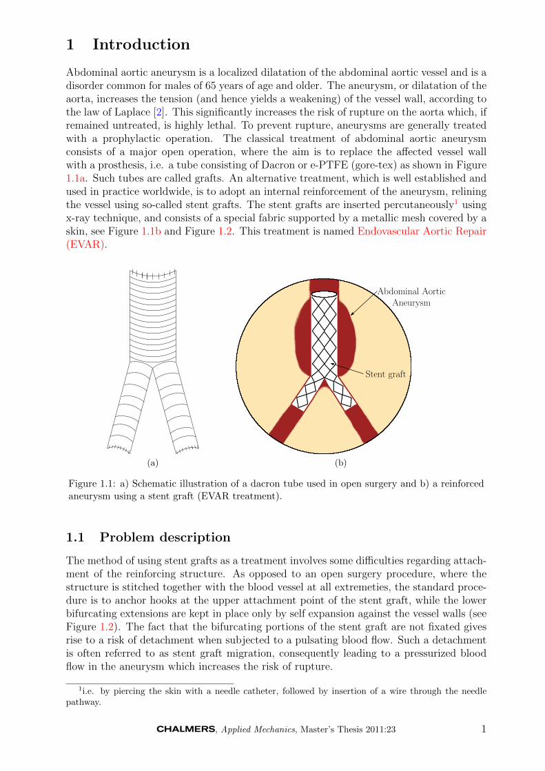
Abdominal aortic aneurysm is a localized dilatation of the abdominal aortic vessel and is adisorder common for males of 65 years of age and older. The aneurysm, or dilatation of theaorta, increases the tension (and hence yields a weakening) of the vessel wall, according tothe law of Laplace [2]. This significantly increases the risk of rupture on the aorta which, ifremained untreated, is highly lethal. To prevent rupture, aneurysms are generally treatedwith a prophylactic operation. The classical treatment of abdominal aortic aneurysmconsists of a major open operation, where the aim is to replace the affected vessel wallwith a prosthesis, i.e. a tube consisting of Dacron or e-PTFE (gore-tex) as shown in Figure1.1a. Such tubes are called grafts. An alternative treatment, which is well established andused in practice worldwide, is to adopt an internal reinforcement of the aneurysm, reliningthe vessel using so-called stent grafts. The stent grafts are inserted percutaneously1 usingx-ray technique, and consists of a special fabric supported by a metallic mesh covered by askin, see Figure 1.1b and Figure 1.2. This treatment is named Endovascular Aortic Repair(EVAR).
(a)
Abdominal AorticAneurysm
Stent graft
(b)
Figure 1.1: a) Schematic illustration of a dacron tube used in open surgery and b) a reinforcedaneurysm using a stent graft (EVAR treatment).
1.1 Problem description
The method of using stent grafts as a treatment involves some difficulties regarding attach-ment of the reinforcing structure. As opposed to an open surgery procedure, where thestructure is stitched together with the blood vessel at all extremeties, the standard proce-dure is to anchor hooks at the upper attachment point of the stent graft, while the lowerbifurcating extensions are kept in place only by self expansion against the vessel walls (seeFigure 1.2). The fact that the bifurcating portions of the stent graft are not fixated givesrise to a risk of detachment when subjected to a pulsating blood flow. Such a detachmentis often referred to as stent graft migration, consequently leading to a pressurized bloodflow in the aneurysm which increases the risk of rupture.
1i.e. by piercing the skin with a needle catheter, followed by insertion of a wire through the needlepathway.
, Applied Mechanics, Master’s Thesis 2011:23 1
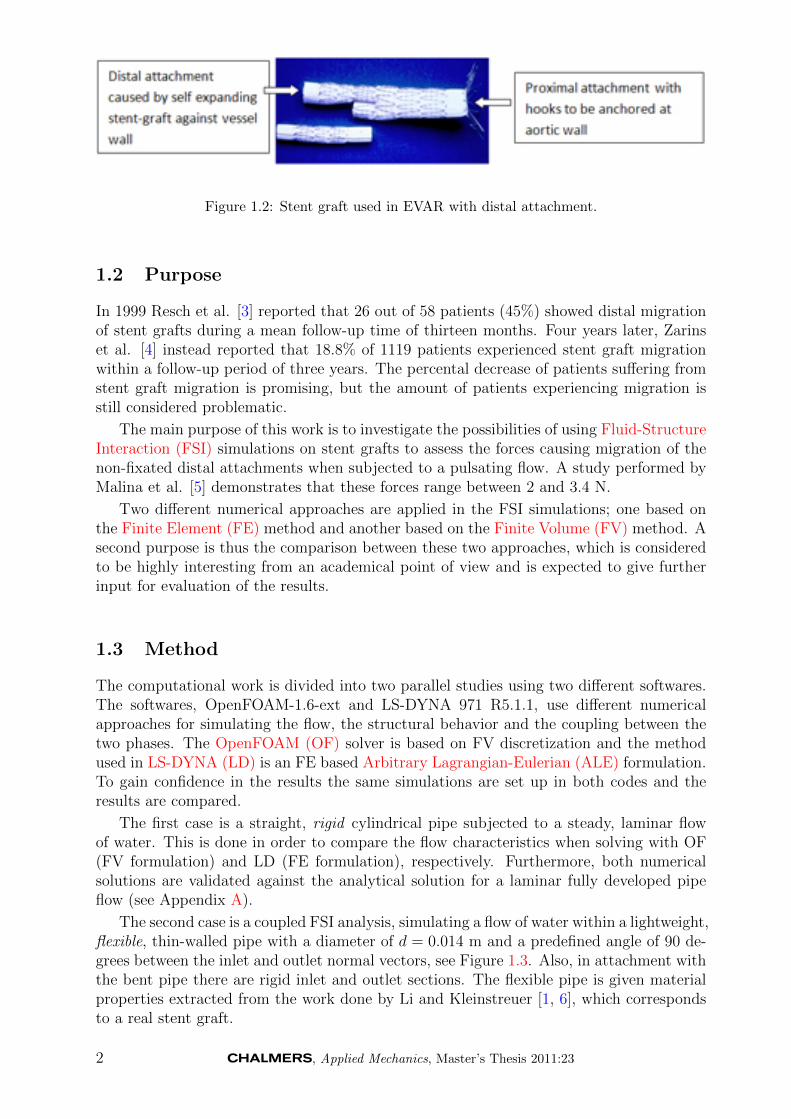
Figure 1.2: Stent graft used in EVAR with distal attachment.
1.2 Purpose
In 1999 Resch et al. [3] reported that 26 out of 58 patients (45%) showed distal migrationof stent grafts during a mean follow-up time of thirteen months. Four years later, Zarinset al. [4] instead reported that 18.8% of 1119 patients experienced stent graft migrationwithin a follow-up period of three years. The percental decrease of patients suffering fromstent graft migration is promising, but the amount of patients experiencing migration isstill considered problematic.
The main purpose of this work is to investigate the possibilities of using Fluid-StructureInteraction (FSI) simulations on stent grafts to assess the forces causing migration of thenon-fixated distal attachments when subjected to a pulsating flow. A study performed byMalina et al. [5] demonstrates that these forces range between 2 and 3.4 N.
Two different numerical approaches are applied in the FSI simulations; one based onthe Finite Element (FE) method and another based on the Finite Volume (FV) method. Asecond purpose is thus the comparison between these two approaches, which is consideredto be highly interesting from an academical point of view and is expected to give furtherinput for evaluation of the results.
1.3 Method
The computational work is divided into two parallel studies using two different softwares.The softwares, OpenFOAM-1.6-ext and LS-DYNA 971 R5.1.1, use different numericalapproaches for simulating the flow, the structural behavior and the coupling between thetwo phases. The OpenFOAM (OF) solver is based on FV discretization and the methodused in LS-DYNA (LD) is an FE based Arbitrary Lagrangian-Eulerian (ALE) formulation.To gain confidence in the results the same simulations are set up in both codes and theresults are compared.
The first case is a straight, rigid cylindrical pipe subjected to a steady, laminar flowof water. This is done in order to compare the flow characteristics when solving with OF(FV formulation) and LD (FE formulation), respectively. Furthermore, both numericalsolutions are validated against the analytical solution for a laminar fully developed pipeflow (see Appendix A).
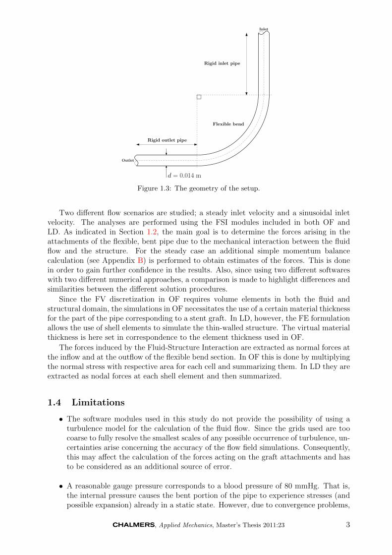
The second case is a coupled FSI analysis, simulating a flow of water within a lightweight,flexible, thin-walled pipe with a diameter of d = 0.014 m and a predefined angle of 90 de-grees between the inlet and outlet normal vectors, see Figure 1.3. Also, in attachment withthe bent pipe there are rigid inlet and outlet sections. The flexible pipe is given materialproperties extracted from the work done by Li and Kleinstreuer [1, 6], which correspondsto a real stent graft.
2 , Applied Mechanics, Master’s Thesis 2011:23
Rigid outlet pipe
Rigid inlet pipe
Flexible bend
Outlet
Inlet
d = 0.014 m
Figure 1.3: The geometry of the setup.
Two different flow scenarios are studied; a steady inlet velocity and a sinusoidal inletvelocity. The analyses are performed using the FSI modules included in both OF andLD. As indicated in Section 1.2, the main goal is to determine the forces arising in theattachments of the flexible, bent pipe due to the mechanical interaction between the fluidflow and the structure. For the steady case an additional simple momentum balancecalculation (see Appendix B) is performed to obtain estimates of the forces. This is donein order to gain further confidence in the results. Also, since using two different softwareswith two different numerical approaches, a comparison is made to highlight differences andsimilarities between the different solution procedures.
Since the FV discretization in OF requires volume elements in both the fluid andstructural domain, the simulations in OF necessitates the use of a certain material thicknessfor the part of the pipe corresponding to a stent graft. In LD, however, the FE formulationallows the use of shell elements to simulate the thin-walled structure. The virtual materialthickness is here set in correspondence to the element thickness used in OF.
The forces induced by the Fluid-Structure Interaction are extracted as normal forces atthe inflow and at the outflow of the flexible bend section. In OF this is done by multiplyingthe normal stress with respective area for each cell and summarizing them. In LD they areextracted as nodal forces at each shell element and then summarized.
1.4 Limitations
• The software modules used in this study do not provide the possibility of using aturbulence model for the calculation of the fluid flow. Since the grids used are toocoarse to fully resolve the smallest scales of any possible occurrence of turbulence, un-certainties arise concerning the accuracy of the flow field simulations. Consequently,this may affect the calculation of the forces acting on the graft attachments and hasto be considered as an additional source of error.
• A reasonable gauge pressure corresponds to a blood pressure of 80 mmHg. That is,the internal pressure causes the bent portion of the pipe to experience stresses (andpossible expansion) already in a static state. However, due to convergence problems,
, Applied Mechanics, Master’s Thesis 2011:23 3
this pressure condition is not taken into account in the simulations. Hence, the forcesextracted from the computational analyses are induced only by the fluid motion.
1.5 Assumptions and simplifications
• In order to achieve managable calculation times, a symmetry condition is introducedfor the setups in both softwares. The use of symmetry is argued to be applicablesince the solution for a laminar pipe flow should be symmetric. Moreover, in caseof occurence of turbulence the symmetry condition is considered not to give rise tomore sources of errors than the already insufficiently resolved turbulence.
• The calculations are performed using water as the fluid medium.
• A bulk modulus for water of the magnitude 106 is assumed to be adequate to avoidcompressibility effects in LD.
• Only one of the distal extensions is simulated.
• The geometry is generalized in such a way that the curvature of the bent pipe isassumed to be circular and, as mentioned in Section 1.3, the angle between the inletand outlet normal vectors is set to 90 degrees.
• The sinusoidal flow is assumed to pulsate with a frequency corresponding to a heartrate of 60 bpm.
• The structure is considered to be in an initial stressfree state. That is, stresses thatarise due to the initial bending of the pipe are neglected in the analysis.
• The flexible pipe material is assumed to have a constant density, i.e. not dependentupon the stretching or compression of the material.
• Modelling a woven stent graft material with a reinforcing structure is consideredtoo complex and time consuming. Hence, the pipe walls are modelled as smooth.Moreover, the material is considered both isotropic and homogeneous, disregardingany anisotropy present due to a stented structure. For this reason, the flexible pipeis from now on referred to as an Endovascular Graft (EVG).
1.6 Sustainability and environmental aspects
If the knowledge from this project (as well as subsequent ones) leads to improvementslowering the percentage of patients experiencing stent graft migration and reducing thenumber of fatalities, this is of great weight from a sustainability point of view. Withfurther confidence in the stent graft’s performance, there can be a reduced amount offollow up sessions and emergency surgeries, lowering the overall material cost and in thelong run lessening the impact on the environment.
4 , Applied Mechanics, Master’s Thesis 2011:23

2 Theory
This section presents a general overview of some fundamental concepts of continuum me-chanics along with basic notations, followed by more detailed explanations of the theorybehind the FE based ALE approach used in LD as well as the FV formulation used in theOF solver.
2.1 Notations
Consider three domains (see Figure 2.1), the spatial domain (B), the material domain (B0)and the arbitrary referential domain (B). Let t denote the open time interval t ∈ ]0, T [ andlet X, X and x denote the material, referential and spatial coordinates. A time derivativeof some function ζ is required in order to describe the continuum, where ζ can be definedas a function of previous mentioned coordinates. Hence [7]:The spatial time derivative
dζ
dt=∂ζ(x, t)
∂t|x (2.1)
The material time derivative
ζ =dζ(X, t)
dt|X (2.2)
The referential time derivative
ζ =dζ(X, t)
dt|X (2.3)
The spatial domain, and the image of Bo at time t, is defined through the material mapϕ. Assume B to be the image of B at time t under the mesh map ϕ. The material motionis characterized through the material map ϕ from the material configuration B0 to spatialconfiguration B with:
x = ϕ(X, t) : B0 → B,
its linear tangent map:
F = ∇Xϕ(X, t) : TB0 → TB,
and its Jacobian:
J = det F.
The Jacobian define the following relations between spatial and material vectorial areaelements and infinitesimal volume elements respectively:
da = JF−T · dA, dv = JdV.
Similarly, the vector map ϕ from the referential B to the spatial B configuration, withthe mesh motion characterized by:
x = ϕ(X, t) : B → B
and its related linear tangent map and Jacobian:
F = ∇Xϕ(X) : TB → TB, J = det F.
, Applied Mechanics, Master’s Thesis 2011:23 5
The Jacobian is used to define the following relations between spatial and referential vec-torial area and volume elements as:
da = JF−T · dA, dv = JdV .
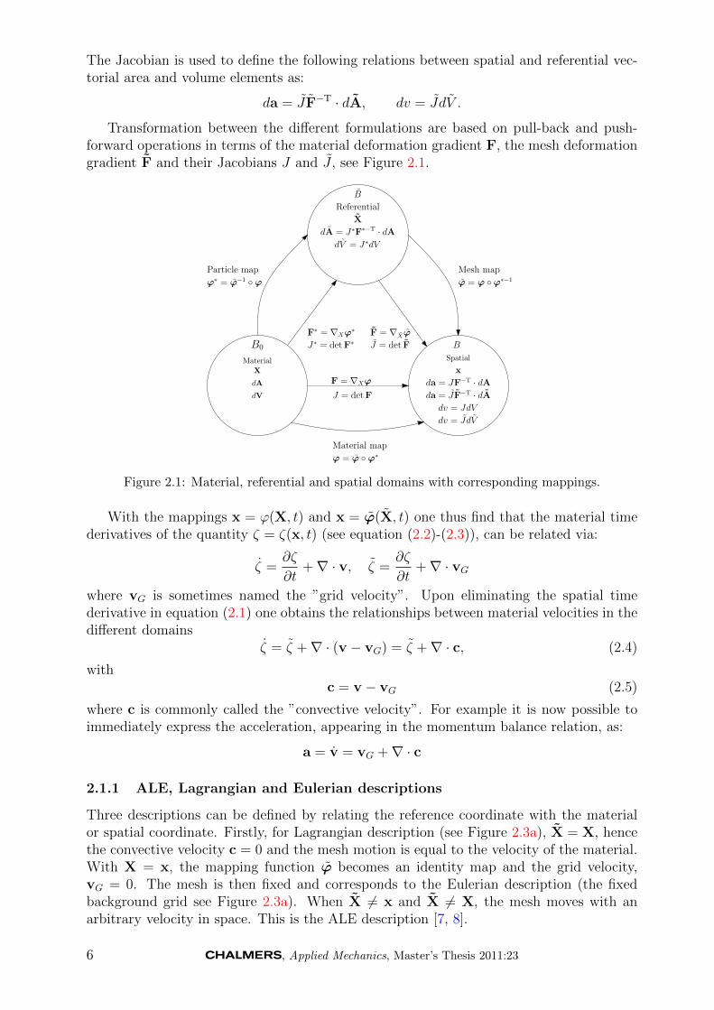
Transformation between the different formulations are based on pull-back and push-forward operations in terms of the material deformation gradient F, the mesh deformationgradient F and their Jacobians J and J , see Figure 2.1.
B0
Material
X
dA
dV
Particle map
ϕ∗ = ϕ−1 ◦ϕ
B
X
Referential
dA = J∗F∗−T · dAdV = J∗dV
Mesh map
ϕ = ϕ ◦ϕ∗−1
Material map
ϕ = ϕ ◦ϕ∗
F∗ = ∇Xϕ∗ F = ∇Xϕ
J∗ = detF∗ B
Spatial
x
da = JF−T · dAda = JF−T · dA
dv = JdV
dv = JdV
J = det F
F = ∇Xϕ
J = detF
Figure 2.1: Material, referential and spatial domains with corresponding mappings.
With the mappings x = ϕ(X, t) and x = ϕ(X, t) one thus find that the material timederivatives of the quantity ζ = ζ(x, t) (see equation (2.2)-(2.3)), can be related via:
ζ =∂ζ
∂t+∇ · v, ζ =
∂ζ
∂t+∇ · vG
where vG is sometimes named the ”grid velocity”. Upon eliminating the spatial timederivative in equation (2.1) one obtains the relationships between material velocities in thedifferent domains
ζ = ζ +∇ · (v − vG) = ζ +∇ · c, (2.4)
withc = v − vG (2.5)
where c is commonly called the ”convective velocity”. For example it is now possible toimmediately express the acceleration, appearing in the momentum balance relation, as:
a = v = vG +∇ · c
2.1.1 ALE, Lagrangian and Eulerian descriptions
Three descriptions can be defined by relating the reference coordinate with the materialor spatial coordinate. Firstly, for Lagrangian description (see Figure 2.3a), X = X, hencethe convective velocity c = 0 and the mesh motion is equal to the velocity of the material.With X = x, the mapping function ϕ becomes an identity map and the grid velocity,vG = 0. The mesh is then fixed and corresponds to the Eulerian description (the fixedbackground grid see Figure 2.3a). When X 6= x and X 6= X, the mesh moves with anarbitrary velocity in space. This is the ALE description [7, 8].
6 , Applied Mechanics, Master’s Thesis 2011:23

2.2 Physical conservation principles
Consider an isothermal continuum element in an arbitrary volume V bounded by a surfaceS at a time t. The continuum is then governed by the fundamental conservation laws formass and linear momentum [9], i.e:
d
dt
∫
V
ρ dV = 0, (2.6)
d
dt
∫
V
ρv dV =
∫
V
ρb dV +
∫
S
t(nf ) dS (2.7)
where ρ is the continuum density (whether it is a fluid or solid constituent), v is theconstituent velocity which, pertinent to a Cartesian coordinate system with basis vectorsin the Eulerian frame [ei]i=x,y,z, take on the components [vi]i=x,y,z. Moreover, b is the bodyforce vector with components [bi]i=x,y,z and t(nf ) is the vectorial force per unit surface areaacting on the boundary S.
By using Reynold’s transport theorem, i.e.
d
dt
∫
V
φ dV =
∫
V
(∂φ
∂t+∇ · (φv)
)dV (2.8)
with φ = φ(x, t) being an arbitrary spatial quantity, the law of mass conservation (2.6) canbe written as ∫
V
(∂ρ
∂t+∇ · (ρv)
)dV = 0 (2.9)
where ∇ is the spatial vector gradient operator with components [∇i]i=x,y,z =[∂∂x, ∂∂y, ∂∂z
].
The Cauchy stress theorem states that there exists a second order tensor σ related to thetraction such that
t(nf ) = σ · nf (2.10)
where nf is the outwards pointing unit normal vector of the outer surface. The tensor σis called the Cauchy stress tensor. By using relation (2.10) together with the divergencetheorem, the right hand side of the momentum conservation law (equation (2.7)) can berewritten. By also introducing Reynold’s transport theorem and cancelling out the zerovalue terms due to mass conservation (equation (2.9)), the momentum equation can beexpressed as
d
dt
∫
V
ρv dV =
∫
V
(σ · ∇+ ρb) dV. (2.11)
2.2.1 Viscous fluids
For an infinitesimal fixed isothermal Control volume (CV) dV , (see Figure 2.2) localizationof equation (2.9) yields that
∂ρ
∂t+∇ · (ρv) = 0 (2.12)
Equation (2.12) is the continuum version of the mass conservation equation and is oftenreferred to as the equation of continuity.
, Applied Mechanics, Master’s Thesis 2011:23 7

y
z
x
Control volume
dy
dx
dz
Figure 2.2: An infinitesimal control volume dV .
By using a similar reasoning for the conservation of momentum, the differential mo-mentum equation for an infinitesimal CV (in vector form) read
d
dt(ρv) = σ · ∇+ ρb (2.13)
where dvdt
= ∂v∂t
+ v · ∇v is the material derivative.The general assumption for fluids is that the stress is a function of pressure and the
velocity gradient [9], i.e.σ = σ(p,∇v)
and the constitutive relation for a viscous fluid is usually assumed to be additativelydecomposed according to
σ = −pI + τ . (2.14)
Introducing (2.14) into (2.13) yields the differential momentum equations for a viscousfluid as
d
dt(ρv) = −∇p+∇ · τ + ρb (2.15)
where ∇p is the pressure gradient across the CV and τ is the viscous stress tensor definedas
τ =
τxx τxy τxzτyx τyy τyzτzx τzy τzz
. (2.16)
The viscous stresses can be written as [10]
τxx = 2µ∂vx∂x, τyy = 2µ∂vy
∂y, τzz = 2µ∂vz
∂z,
τxy = τyx = µ(∂vx∂y
+ ∂vy∂x
), τxz = τzx = µ
(∂vz∂x
+ ∂vx∂z
), τyz = τzy = µ
(∂vy∂z
+ ∂vz∂y
)
(2.17)
8 , Applied Mechanics, Master’s Thesis 2011:23
where µ is the coefficient of dynamic viscosity. Substituting (2.17) into (2.15) gives thedifferential momentum equation for a Newtonian fluid2 as
d
dt(ρv) = −∇p+ µ∇2v + ρb. (2.18)
Equation (2.18) is more commonly known as the Navier-Stokes equation.
2.2.2 Elastic solids
For an elastic solid the Cauchy stress is a function of the displacement gradient [9], i.e.
σ = σ(∇u)
where u = r − r0 denotes the displacement vector relating the current material pointposition, r, to the initial material point position, r0. Since the solid is assumed to beelastically compressible, the pressure is also a function of ∇u and is hence not needed asan argument for the stress.
When considering finite deformations, alternatives to the Cauchy stress tensor are oftenused. The Piola-Kirchhoff stress tensors are examples of such alternatives. They expressthe stress relative to a reference configuration, whereas the Cauchy stress tensor expressesthe stress in relation to the present configuration.
The first Piola-Kirchhoff stress tensor, P , relates forces in the present configurationwith areas in the reference (”material”) configuration. The first Piola-Kirchhoff stresstensor is related to the Cauchy stress tensor as
P = Jσ · F−T (2.19)
where F is the deformation gradient tensor defined as
F = I + (∇Xu)T (2.20)
where ∇X = ∇ · F−T is the material gradient operator.The second Piola-Kirchhoff stress tensor, Σ, is further defined in terms of the first
Piola-Kirchhoff stress tensor asΣ = F−1 ·P (2.21)
and the relation between the second Piola-Kirchhoff stress tensor and the Green-Lagrangianstrain tensor is governed by the constitutive equation for a St. Venant-Kirchhoff material,i.e.
Σ = 2GE + λ tr (E)I (2.22)
where G and λ are the Lame’s coefficients and E is the Green-Lagrangian strain tensordefined as
E =1
2(FT · F− I). (2.23)
Once again, using localization, equation (2.11) can now be expressed in terms of the firstor the second Piola-Kirchhoff stress tensor as
ρ0dv
dt= P · ∇X + ρ0b (2.24)
and
ρ0dv
dt= (F ·Σ) · ∇X + ρ0b. (2.25)
2i.e. a fluid that follows the linear law of resistance, τ = µdvx
dy , postulated by Sir Isaac Newton in 1687.
, Applied Mechanics, Master’s Thesis 2011:23 9
2.3 Numerical approaches in LS-DYNA and OpenFOAM
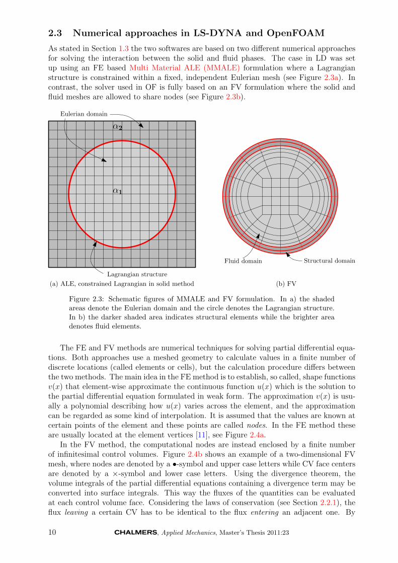
As stated in Section 1.3 the two softwares are based on two different numerical approachesfor solving the interaction between the solid and fluid phases. The case in LD was setup using an FE based Multi Material ALE (MMALE) formulation where a Lagrangianstructure is constrained within a fixed, independent Eulerian mesh (see Figure 2.3a). Incontrast, the solver used in OF is fully based on an FV formulation where the solid andfluid meshes are allowed to share nodes (see Figure 2.3b).
α1
α2
Lagrangian structure
Eulerian domain
(a) ALE, constrained Lagrangian in solid method
Fluid domain Structural domain
(b) FV
Figure 2.3: Schematic figures of MMALE and FV formulation. In a) the shadedareas denote the Eulerian domain and the circle denotes the Lagrangian structure.In b) the darker shaded area indicates structural elements while the brighter areadenotes fluid elements.
The FE and FV methods are numerical techniques for solving partial differential equa-tions. Both approaches use a meshed geometry to calculate values in a finite number ofdiscrete locations (called elements or cells), but the calculation procedure differs betweenthe two methods. The main idea in the FE method is to establish, so called, shape functionsv(x) that element-wise approximate the continuous function u(x) which is the solution tothe partial differential equation formulated in weak form. The approximation v(x) is usu-ally a polynomial describing how u(x) varies across the element, and the approximationcan be regarded as some kind of interpolation. It is assumed that the values are known atcertain points of the element and these points are called nodes. In the FE method theseare usually located at the element vertices [11], see Figure 2.4a.
In the FV method, the computational nodes are instead enclosed by a finite numberof infinitesimal control volumes. Figure 2.4b shows an example of a two-dimensional FVmesh, where nodes are denoted by a •-symbol and upper case letters while CV face centersare denoted by a ×-symbol and lower case letters. Using the divergence theorem, thevolume integrals of the partial differential equations containing a divergence term may beconverted into surface integrals. This way the fluxes of the quantities can be evaluatedat each control volume face. Considering the laws of conservation (see Section 2.2.1), theflux leaving a certain CV has to be identical to the flux entering an adjacent one. By
10 , Applied Mechanics, Master’s Thesis 2011:23

discretizing the surface integrals [12], and assuming that the rate of change is polynomialacross the cell, the fluxes can then be used to evaluate the sought after variables in eachnode.
(i, j + 1) (i+ 1, j + 1)
(i, j) (i+ 1, j)
x, y,v
p, V, ρ,m(i+ 1
2, j + 1
2
)
(a) Four-noded FE element: variable positionscorresponding to the ALE formulation.
PW E
N
S SESW
NENW
w e
n
s
(b) Structured 2D FV mesh: velocities and pres-sure computed in nodes (•), fluxes computed atcontrol volume surfaces (×).
Figure 2.4: Schematic figures of FE and FV formulation.
Since the applied ALE formulation is based on an FE approach the element nodesare positioned at the element vertices (see Figure 2.4a). These nodes contain the meshcoordinates, x and y, and the velocity, v. The mass, m, and volume, V , are instead definedin the center of the element,
(i+ 1
2, j + 1
2
), where also the pressure, p, and the material
density, ρ, are calculated.Each of the element solution variables have to be transported. Since the velocities are
stored in the element vertices and the density is stored in the element center, this givesrise to difficulties of advecting the momentum (which is a product of density and velocity).In this ALE approach these difficulties are overcome by advecting the nodal momentuminstead of the velocity, in order to ensure conservation of momentum [13]. The procedureis to modify an element-centered advection algorithm to advect the node-centered momen-tum. This is done by constructing auxiliary sets of element-centered variables from the(nodal) momentum, advect them and then reconstruct the new (nodal) velocities from theauxiliary variables.
The chosen ALE method (MMALE, see Section 2.4) demands two or more materialsto be defined within the Eulerian mesh; the first one, α1, in the elements constrained bythe Lagrangian structure and a second one, α2, in the surronding elements. This is notthe case in OF where the calculations are performed for a single fluid material.
Since the Eulerian and Lagrangian meshes are not coupled nodewise in LD, a couplingalgorithm is needed to define the contact interfaces between the Lagrangian mesh and thematerials defined in the Eulerian mesh. There are several coupling methods applicable forthe ALE formulation. In LD both penalty based and constraint based coupling methodsare available. Thus, a brief description of the two approaches is provided in Section 2.4.
In OF the coupling between the phases is governed by a traction vector, consistingof the fluid pressure and the shear stresses arising from the fluid-structure interaction.The traction vector is obtained by calculating the flow field and is then introduced into
, Applied Mechanics, Master’s Thesis 2011:23 11
the equations for the structure. Subsequently, the structural displacements are solved forand both the fluid and solid meshes are deformed accordingly. The displacement of thefluid-structure interface then appears as a boundary condition for the fluid phase in thefollowing time step and the solution procedure is repeated.
2.4 The Arbitrary Lagrangian-Eulerian formulation in LS-DYNA
In fluid-structure interaction problems where the fluid mesh, if treated as Lagrangian,would undergo massive deformation near the structure, causing the timestep to take anunacceptable small value, ALE is of great use [13]. The method is sometimes used to createa new undistorted mesh for the deforming domain which makes it possible to continue thecalculations. In the case of the EVG, the structure is treated as a Lagrangian and the fluidas a fixed Eulerian mesh. This way any distortions of the fluid mesh due to displacementof the EVG structure is completely avoided. The details of LD’s ALE implementation arenot fully available. Nevertheless, a conceptual overview is provided in this section.
2.4.1 Governing equations
The chosen method in LD solves the isothermal fluid problem using Eulerian descrip-tions of the continuity equation and the Navier-Stokes equations (see equation (2.12) and(2.18)) discussed in section 2.2.1. That is, the grid velocity is zero and hence, according toequation (2.5), the convective velocity equals the material velocity, i.e. c = v. Neglectingall the body forces, the governing equations for the compressible fluid problem then become
Continuity equation∂ρ
∂t+∇ · (ρv) = 0 (2.26)
Momentum equationd
dt(ρv) = −∇p+ µ∇2v in B (2.27)
The governing equation for the structural behavior, expressed in the Lagrangian framework,is the conservation of momentum:
ρ0dv
dt= P · ∇X + ρ0b in B0 (2.28)
where P is the first Piola-Kirchhoff stress tensor (see equation (2.19) in Section 2.2.2).
2.4.2 Multi Material ALE
In Eulerian and ALE-formulation it is possible to allow two or more materials in oneelement in a fixed mesh. In LD this is refereed to as the Multi Material ALE (MMALE)method where the elements contain a certain volume fraction of each material. The volumefraction represented by αei in element e of material i is expressed as:
αei =V ei
V e(2.29)
where V ei represents the material volume and Vi the element volume. Furthermore the sum
of the volume fractions must always equal 1 within one element such that:
n∑
i=1
αei = 1 (2.30)
12 , Applied Mechanics, Master’s Thesis 2011:23
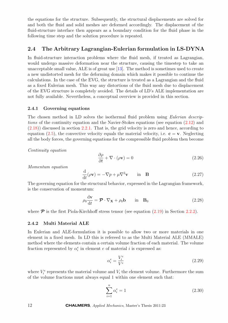
As the mass fluxes between elements, the initially well defined material boundary is re-placed by a transition region where αei drops from 1 to 0. If the interface was to be trackedby either the donor cell or van Leer advection scheme, it would be severely smeared [14].Instead interface reconstruction is used, where the mixed elements are cut with a planeseparating the materials (see Figure 2.5). The orientation of the plane is controlled by thegradient of the volume fraction field, which is governed by the Lagrangian structure. Whenthe structure moves, the volume fractions are updated and the interface plane is recon-structed accordingly. The movement of the structure is determined by the fluid structureinteraction, for which a coupling algorithm is needed.
αn=31 = 0.7 αn=4
1 = 0.5
αn=11 = 0.5 αn=2
1 = 0.2
α1 = 0.8
α2 = 0.2 V
n
α1V
α2V
n =∣∣∣∣∣∣∂α1∂x
∣∣∣∣∣∣ · ∂α1
∂x = 1√2
{11
}
Figure 2.5: MMALE with two materials.
2.4.3 Fluid-structure interaction
The most fundamental question when dealing with fluid-structure interaction is arguablywhether the fluid and structural parts are in contact with eachother. This section presentsthe basics of the contact based methods, regarding the fluids and solids as compounds ofparticles. LD does not treat the phases as compounds of particles; instead the couplingis handled by nodal contacts. However, the concept of the coupling is similar, consideringthe nodes as particles. Hence, the following reasoning is considered valid for explaining themain idea behind the coupling methods.
The conditions for finding possible collisional contacts between particles can be writtenas [15]
||Xf −Xs|| ≤ rf + rs (2.31)
andn · (vf − vs) ≤ 0 (2.32)
where Xf and Xs denote the positions of the fluid and solid particles, respectively, rf andrs denote their radii, n is the unit surface normal at the contact point and vf and vsrepresent the fluid and solid velocities, respectively.
, Applied Mechanics, Master’s Thesis 2011:23 13

vf
vs
n
rf
rs
Xf
Xs
Xp
Xc
r
Figure 2.6: Collision between fluid and solid particles.
Figure 2.6 shows a collision between a fluid and solid particle. The solid particle velocityis expressed as vs = vpar +ω× r, where vpar and ω are the linear and angular velocities ofthe corresponding solid particle, respectively.
From Figure 2.6 and equation (2.31) it can be concluded that the fluid and solid particlesoverlap eachother at the contact point Xp = Xs + rsn. Equation (2.32) then implies thatthe relative velocity of the fluid particle with respect to the solid particle along the normaldirection is less than zero. A positive value of the relative velocity would instead mean thatthe particles are no longer interpenetrated. This would be the case in a future time stepwhen the particles would be separated and hence not in contact with eachother anymore.
To resolve all contacts between the fluid and solid phases a coupling algorithm is needed.LD offers a penalty based coupling method as well as a constraint based one. The penaltybased method computes contact forces, Fcontact, between the fluids and solids to preventthe interpenetration of the phase surfaces. The contact force is defined as
Fcontact = ksdn + kd(vrel · n)n (2.33)
where ks and kd represent the stiffness and damping coefficients respectively, d denotesthe penetration depth or the overlap between the colliding surfaces, n is the unit surfacenormal at the contact point and vrel is the relative velocity between the fluid and solidnodes.
Finding a suitable value for the stiffness parameter can be somewhat troublesome andis a matter of trial and error. Another shortcoming with the penalty based method is thatit requires very small time steps to stably resolve collisions.
The constraint based coupling method provides another way to resolve the fluid-solidcontacts. This method connects the velocities of the fluid and solid bodies through animpulse description, rather than affecting their accelerations through a contact force. Un-like the penalty based method, the constraint based method does not conserve the kineticenergy [14]. Figure 2.7 shows a conceptual explanation of the constraint based couplingmethod used in LD where a collision between the phases is considered perfectly inelastic.
m m
vfluid solid
(a) Before impact
12v
12v
(b) After impact
Figure 2.7: Schematic figures of a fluid particle a) before and b) after colliding witha solid particle for the constraint based coupling method used in LD.
14 , Applied Mechanics, Master’s Thesis 2011:23

Before impact of the fluid and solid particles (see Figure 2.7a) the momentum, p, andkinetic energy, Wk, are
p0 = mv (2.34)
Wk0 =1
2mv2 (2.35)
where subscripts 0 refers to values at time t = 0, i.e. before impact.After a perfectly inelastic collision (see Figure 2.7b), the particles stick together with
a conserved momentum
p1 =1
2mv +
1
2mv = mv = p0, (2.36)
but with a loss in kinetic energy
Wk1 =1
4mv2 < Wk0 . (2.37)
2.4.4 Solution procedure of the LS-DYNA solver
A non-symmetric convective term, stemming from the convective velocity c, poses majordifficulties associated with time integration. If considering a Lagrangian description therelative motion is zero due to the material and referential systems being identical and thusthe convective term would disappear. In order to solve the ALE equations LD applies theOperator Split method. The approach is used in order to achieve less complex problems,divided into two or more sets which are solved sequentially.
The structural equations (2.28) are solved with the fluid pressure and shear stressesfrom equation (2.27) on the interface as a Neumann boundary condition. The solutiongives the structural velocities which are equal to the grid velocity, vG. The structure’s newposition updates the interface with the volume fractions for the fluid materials.
1. Perform a Lagrangian time step
2. Perform an advection step.
i) Move the material interface.
ii) Calculate the transport of element-centred variables
iii) Calculate the momentum transport and update the velocity.
In the first substep, the mesh moves with the material and the changes in velocity andinternal energy due to internal and external forces are calculated. When the new configura-tion for the Lagrangian substep is reached the advection (or Eulerian) substep takes place.Now a new nodal pattern has to be defined, unless it has been predefined by the user, asis the case for this study, where Eulerian formulation is used and the mesh displacementsset to zero. When the nodal pattern has been defined, the solutions variables need to beremapped to the arbitrary position with an advection algorithm, computing the transportof mass, internal energy and momentum across cell boundaries.
2.4.5 Advection method
When the nodal repositioning has been performed, the solution from the previous, distortedconfiguration need to be mapped onto the new one [14]. This is known as the advectionstep. Two assumptions are made for the remap step, first of all, the topology of the meshis fixed and secondly, during a step, the mesh motion is less than the characteristic lengths
, Applied Mechanics, Master’s Thesis 2011:23 15

of the neighbouring elements, i.e the Courant-Friedrichs-Lewy (CFL) number, should beless than one [13]. The algorithms used to perform the remap step are called advectionalgorithms referring to the scalar conservation equation (2.38):
∂φ
∂t+ a(x)
∂φ
∂t= 0 (2.38)
A beneficial advection algorithm is stable, conservative, accurate and monotonic. Al-though several of the solution variables are not governed by conservation equations, it isvital that they remain unchanged during the remap step. Conservation of mass and energyis particularly important since negative values would lead to non-physical results. The cal-culations for the transport of element centered variables (such as internal energy, the stresstensor, density and history variables) in LD is performed in accordance with the SALE3Dstrategy [16], and in this work using the Monotone Upwind Schemes for Conservation Laws(MUSCL) Van Leer scheme to achieve second order accurate monotonic results.
The fact that the velocities are located at the nodal points and not centered in theelement (see Section 2.3), means that they must be advected separately. Furthermore, themomentum has to be conserved during this process and is a product of the element centereddensity and the nodal velocities. For the momentum transport, a more expensive methodthan SALE, the Half Index Shift (HIS) algorithm is used. This method was developed byD. J. Benson [17] in order to overcome the dispersion problems with the SALE strategy[13].
2.5 The Finite Volume Method formulation in OpenFOAM
The solver used in the OF simulations is an extension of the icoFsiFoam solver and uses anFV formulation for both the fluid and the structural solution of the coupled FSI analysis.The part of the FSI solver that handles the calculation of the flow is based on the standardOF solver icoFoam, which solves the incompressible laminar Navier-Stokes equations usingthe Pressure-Implicit Split-Operator (PISO) algorithm, while the mathematical descriptionbehind the structural solution procedure is based on an updated Lagrangian formulation.
2.5.1 Mathematical formulation of the fluid analysis
The mathematical description behind the fluid analysis in OF is based on the Euleriandifferential approach for fluid flow described in Section 2.2.1. However, some assumptionsand simplifications are made for the equations that are worth mentioning. First of all, anyeffects of gravity or other body forces are neglected throughout the entire analysis, makingthe body force vector disappear from the momentum equations. Secondly, the solver usedin OF assumes that the fluid is incompressible. Hence the density is moved out of theconvective term of equation (2.18), giving
dv
dt= −1
ρ∇p+ ν∇2v. (2.39)
where ν = µ/ρ is the kinematic viscosity. Equations (2.39) are the incompressible Navier-Stokes equations that are solved in OF.
2.5.2 Mathematical formulation of the structural analysis
The majority of the changes in the extension of icoFsiFoam concerns the description ofthe solid phase. This is because the extended version is based on the updated Lagrangian
16 , Applied Mechanics, Master’s Thesis 2011:23
formulation and the mathematical description of this approach is thoroughly explainedin the work done by Tukovic and Jasak [18]. In order to provide a good insight to thisformulation the main contents of their work is also included in this section.
The mathematical description of the structural analysis is based on the conservationprinciples introduced in Section 2.2. Moreover, solving flow problems in a deforming controlvolume requires a mathematical description of the relationship between the rate of changeof the volume V and the motion of its surface, vs. This definition is called the spaceconservation law and is defined as
d
dt
∫
V
dV −∮
S
n · vs dS = 0 (2.40)
Considering an isothermal continuum in an arbitrary volume V bounded by a surface S,the motion is hence governed by the conservation laws of mass and linear momentum, i.e:
d
dt
∫
V
ρ dV +
∮
S
n · ρ(v − vs) dS = 0 (2.41)
d
dt
∫
V
ρv dV +
∮
S
n · ρ(v − vs)v dS =
∮
S
σ · n dS +
∫
V
ρb dV (2.42)
where n is the outward pointing unit normal to the surface S, v is the velocity of thecontinuum, vs is the velocity of the surface S, σ is the Cauchy stress tensor and b is theresulting body force. The difference v − vs can be compared to the convective velocity c(equation (2.5)) discussed in Section 2.1, indicating that the mathematical formulation isin line with an ALE description taking into account the deforming mesh motion.
Assuming an elastic, isothermal structure the dynamic behavior can be described byconsidering only the linear momentum conservation law in Lagrangian formulation, i.e.
D
Dt
∫
V
ρv dV =
∮
S
σ · n dS +
∫
V
ρb dV (2.43)
This can also be expressed in terms of the initial, undeformed control volume as
∫
V0
ρ0∂v
∂tdV0 =
∫
S0
(F ·Σ) · n0 dS0 +
∫
V0
ρ0b dV0 (2.44)
where the subscripts 0 denote quantities related to the initial, undeformed control volume,Σ is the second Piola-Kirchhoff stress tensor (see equation (2.21)) and F is the deformationgradient tensor (see Section 2.2.2).
Equation (2.44), which describes the total linear momentum conservation in Lagrangianformulation, can be written in an incremental form as
∫
V0
ρ0∂δv
∂tdV0 =
∫
S0
(δF ·Σ + F · δΣ) · n0 dS0 +
∫
V0
ρ0δb dV0 (2.45)
where δ represents the increment of the corresponding variables and the deformation gra-dient tensor increment reads δF = (∇δu).
As previously mentioned, the mathematical approach is based on an updated Lagrangianformulation. This means that the reference configuration is continuously updated to (repli-cate) the latest calculated configuration. The corresponding incremental version of equa-tion (2.22) becomes
δΣ = 2GδE + λ tr (δE)I (2.46)
, Applied Mechanics, Master’s Thesis 2011:23 17

where δE is the increment of the Green-Lagrangian strain tensor for the total Lagrangiandescription and is defined as
δE =1
2(δFT · F + FT · δF). (2.47)
Finally, it appears that the linear momentum conservation equation for an elastic solidin the updated Lagrangian description, with the displacement vector increment δu as theprimitive variable, can be obtained as:
∫
Vu
ρu∂δv
∂tdVu −
∮
Su
nu · (2G+ λ)∇δu dSu =
∮
Su
nu · q dSu +
∫
Vu
ρuδb dVu (2.48)
where the subscript u corresponds to the updated variables and
q = G(∇δu)T + λ tr (δu)I− (G+ λ)∇δu +G∇δu · (∇δu)T
+1
2λ(∇δu : ∇δu)I + Σu · δuT
u + δΣu · δFTu . (2.49)
The tensor q consists of nonlinear and coupling terms. In order to solve the discretizedequation using a segregated algorithm, these terms are treated explicitly after the dis-cretization. Jasak and Weller [19] claims that the efficiency of the segregated solutionprocedure can be improved by using the diffusivity (2G + λ) in the Laplacian at the left-hand side of equation (2.48).
For a fully defined problem description the domain needs to be specified in both spaceand time, as well as being given proper initial and boundary conditions. The initial condi-tion is simply the specified distribution of δu and δv at time zero, while there are severaltypes of boundary conditions (which can be either constant or time-dependent); fixed dis-placement increment, plane of symmetry, fixed pressure increment, fixed traction incrementand free surface.
The boundary conditions for fixed pressure increment and fixed traction incrementare both implemented as a fixed normal derivative Neumann boundary condition on thedisplacement increment.
2.5.3 Solution procedure of the OpenFOAM solver
The analysis using the FV method requires a discretization of the computational domainin both time and space. The simulation time is split into a finite number of time steps, δt,and the discretized equations are solved in a stepwise manner, time step by time step. Thecomputational space is discretized by splitting it into a finite number of control volumes.
The fluid and structural systems of equations are solved separately and sequentially foreach time step. As previously mentioned, the solution of the flow field is calculated usingthe PISO algorithm; an iterative procedure for solving equations for velocity and pressurefor transient problems [20]. The process is based on first evaluating initial guesses of thepressure and velocity fields using discretized equations of momentum3 and then correctingthem (at least) twice using a discretized pressure correction equation (derived from theequation of continuity). In this work, the discretization of the advection term (in OF) isdone using the linear upwind scheme; a second-order extension of the standard upwindscheme [12]. Once the solution of the flow field has converged the pressure and shear
3There are several numerical schemes available to discretize the momentum equations. The detailsabout these schemes are extensive and hence not provided in this report, but can be found in e.g. Versteeg& Malalasekera [12].
18 , Applied Mechanics, Master’s Thesis 2011:23

stresses are assembled into the traction vector. As described in Section 2.3 the tractionis then introduced into the structural equations. The following numerical evaluation ofthe structural displacements is similarly obtained by solving the system of discretizedlinear momentum conservation equations for an elastic solid in the updated Lagrangiandescription. Finally, the fluid and structural meshes are both moved in accordance withthe calculated displacements. The steps of the solution procedure can be summarized asfollows:
1. Guess velocity and pressure fields
2. Evaluate the guesses of velocity and pressure and correct them until convergence
i) Extract traction vector from the converged flow equation system
ii) Introduce traction vector into structural equations
3. Evaluate the incremental displacements of the structure
4. Move meshes in accordance with structural displacements
i) Extract incremental displacement velocity from the structural solution
ii) Introduce incremental displacement velocity into flow equations
y
z
x
Control volume
dy
dx
dz
P
nffrpE
df
Sf
Figure 2.8: Hexahedral control volume.
Figure 2.8 shows an example of a hexahedral control volume around the computationalpoint P located in the center of the control volume, its face f , its face area Sf , the faceunit normal vector nf and the center point E of the neighboring control volume sharingthe face f .
Since the conservation of linear momentum is described by the incremental updatedLagrangian formulation (equation (2.48)), the computational mesh has to be moved atthe beginning of each time step. This is done by using the displacement increment vector
, Applied Mechanics, Master’s Thesis 2011:23 19

obtained from the previous time step. The cell-centered FV method that is used in OFcalculates the displacement increment at the control volume center. Thus the calculateddisplacement increment must be interpolated onto the control volume vertices to enablethe dynamic mesh movement. This interpolation is done using a weighted averaging inter-polation given by
δup =
∑cwpc
[δuc + (rp − rc) · (∇δu)c + 1
2(rp − rc)
2:(∇∇δu)c]
∑cwpc
, (2.50)
where δup is the displacement increment of vertex p and δrc denotes the displacementincrement at the center of the control volume. The summation is done over all controlvolumes sharing the p vertex and the weighting factor wpc is defined as
wpc =1
|rp − rc|, (2.51)
where rc denotes the position vector of the control volume center and rp is the positionvector of the vertex p.
20 , Applied Mechanics, Master’s Thesis 2011:23

3 Simulation setups
As stated in Section 1.3, the computational work consists of two parallel studies which areperformed using OF and LD. Due to the different numerical approaches the domains haveto differ in some aspects. The following section presents the different setups (e.g. domains,boundary conditions etc.) for the different analyses.
3.1 Material properties
As indicated in Section 1.3 and 1.4 the fluid medium used in the simulations is water.Some properties of interest of water at 20◦C are listed in Table 3.1.
Table 3.1: Some properties of water at room temperature (20◦C) [21, 22].
Density (ρ) Dynamic viscosity (µ) Kinematic viscosity (ν) Speed of sound (vsound)998.2 [kg/m3] 1.005 · 10−3 [kg/(m·s)] 1.004 · 10−6 [m2/s] 1492 [m/s]
The value for speed of sound is used to calculate the bulk modulus (K) of water. Thebulk modulus describes a material’s resistance to undergo compression, i.e. a high bulkmodulus relates to a low compressibility. The speed of sound can be related to the bulkmodulus as [23]
vsound =
√K
ρ(3.1)
and hence the bulk modulus of water at 20◦C becomes
K = ρv2sound ≈ 2.2 · 109 [Pa]. (3.2)
The solver used in LD does not assume an incompressible fluid (as opposed to the solverused in OF). Thus, in order to omit compressibility a bulk modulus is needed to explicitlycommand the LD solver to treat water as an incompressible fluid. Unfortunately, a bulkmodulus as high as in (3.2) results in extensive calculation times. Hence the assumption ismade that a bulk modulus of the magnitude 106 is adequate to avoid any compressibilityeffects in LD.
The material properties for the EVG are more troublesome to determine. No suchinformation is available from the manufacturer. Hence, the material properties has to beextracted and approximated via literature from similar studies. Two such studies wereperformed by Li and Kleinstreuer [1, 6] from which the properties of the EVG material inthe present study are extracted. These are summarized in Table 3.2.
Table 3.2: Material properties of the EVG.
Thickness (h) Young’s modulus (E) Poisson’s ratio (η) Density (ρ)0.003 [m] 10 [MPa] 0.27 [-] 6000 [kg/m3]
, Applied Mechanics, Master’s Thesis 2011:23 21

3.2 Laminar flow in a rigid pipe
To evaluate the two software modules ability to simulate a flow field, a study of a straight,rigid cylindrical pipe subjected to a steady, laminar flow of water is conducted. To gainfurther confidence in the simulations, the results of the study are validated against theanalytical solution for a laminar fully developed pipe flow (see Appendix A).
3.2.1 Geometry
The analysis is performed on a straight, rigid pipe with diameter d = 0.014 m, i.e. thesame diameter as the subsequently analyzed EVG. The length of the pipe is chosen due tothe requirement that the flow has to be fully developed for a certain interval of the pipelength. This requirement has to be fulfilled in order to compare the simulations with theanalytical solution for a laminar fully developed pipe flow. According to [10], the pipelength needed for the flow to reach a fully developed profile, Le, can be related to the pipediameter, d, and the Reynolds number, Red, as
Le ≈ 0.06dRed. (3.3)
The commonly accepted design value for pipe flow transition from laminar to turbulentflow is [10]
Red,crit ≈ 2300. (3.4)
In order to ensure a laminar flow, the inlet velocity condition for the simulations is chosento be v = 0.12 m/s. Considering water (at room temperature) as the fluid medium, thisgive a Reynolds number of
Red =vd
ν≈ 1673. (3.5)
According to equation 3.3 this requires a pipe length, Le, of approximately 1.4 meters forthe flow to reach a fully developed profile. To enable a comparison with the analyticalsolution the pipe length was set to 2 meters.
3.2.2 Mesh
To save computational time, the simulation is done for half the pipe by making use ofsymmetry the same way as for the final EVG case. The mesh topology used is an o-gridwhich is commonly used for pipe flow simulations thanks to its capability of resolving theboundary layer, see Figure 3.1a. The flow is simulated using the FSI solvers (in uncoupledmode). This is because the main reason of the analysis is to compare the solvers and theway they solve the flow field.
22 , Applied Mechanics, Master’s Thesis 2011:23
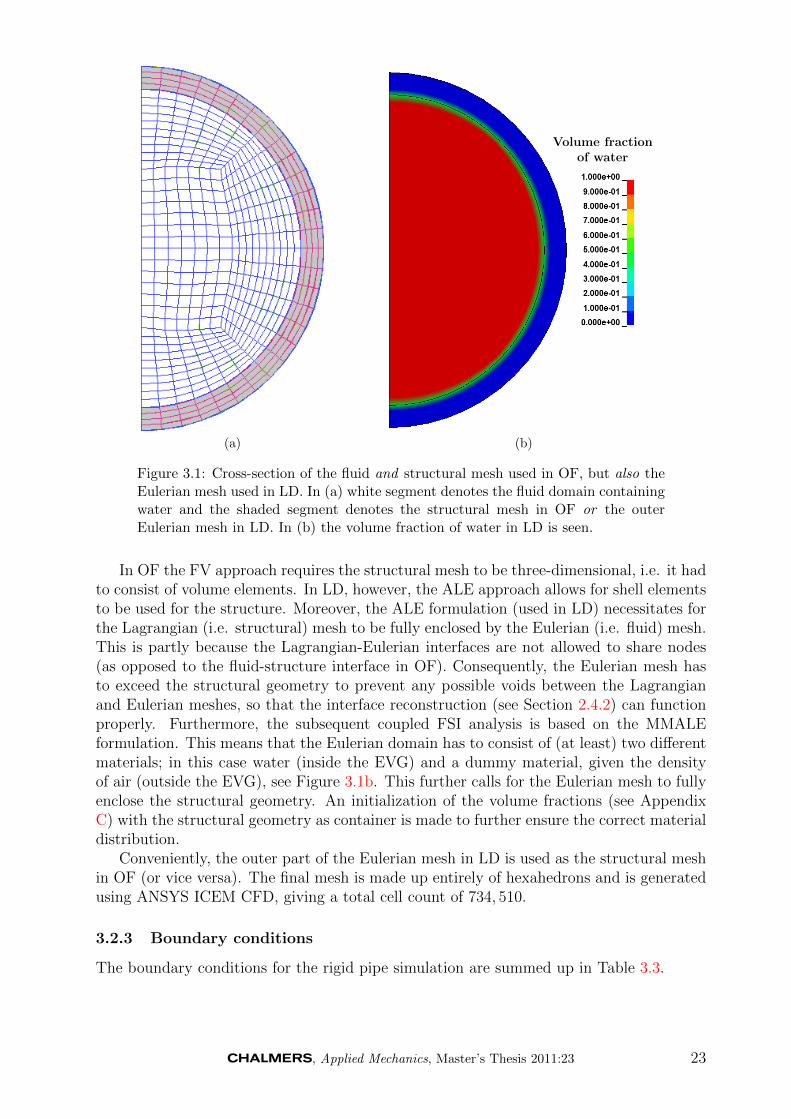
(a)
Volume fractionof water
(b)
Figure 3.1: Cross-section of the fluid and structural mesh used in OF, but also theEulerian mesh used in LD. In (a) white segment denotes the fluid domain containingwater and the shaded segment denotes the structural mesh in OF or the outerEulerian mesh in LD. In (b) the volume fraction of water in LD is seen.
In OF the FV approach requires the structural mesh to be three-dimensional, i.e. it hadto consist of volume elements. In LD, however, the ALE approach allows for shell elementsto be used for the structure. Moreover, the ALE formulation (used in LD) necessitates forthe Lagrangian (i.e. structural) mesh to be fully enclosed by the Eulerian (i.e. fluid) mesh.This is partly because the Lagrangian-Eulerian interfaces are not allowed to share nodes(as opposed to the fluid-structure interface in OF). Consequently, the Eulerian mesh hasto exceed the structural geometry to prevent any possible voids between the Lagrangianand Eulerian meshes, so that the interface reconstruction (see Section 2.4.2) can functionproperly. Furthermore, the subsequent coupled FSI analysis is based on the MMALEformulation. This means that the Eulerian domain has to consist of (at least) two differentmaterials; in this case water (inside the EVG) and a dummy material, given the densityof air (outside the EVG), see Figure 3.1b. This further calls for the Eulerian mesh to fullyenclose the structural geometry. An initialization of the volume fractions (see AppendixC) with the structural geometry as container is made to further ensure the correct materialdistribution.
Conveniently, the outer part of the Eulerian mesh in LD is used as the structural meshin OF (or vice versa). The final mesh is made up entirely of hexahedrons and is generatedusing ANSYS ICEM CFD, giving a total cell count of 734, 510.
3.2.3 Boundary conditions
The boundary conditions for the rigid pipe simulation are summed up in Table 3.3.
, Applied Mechanics, Master’s Thesis 2011:23 23
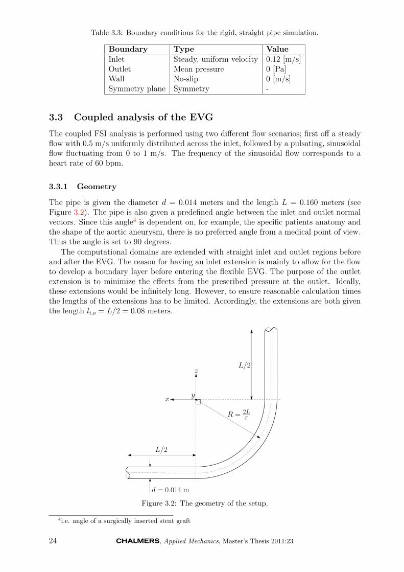
Table 3.3: Boundary conditions for the rigid, straight pipe simulation.
Boundary Type ValueInlet Steady, uniform velocity 0.12 [m/s]Outlet Mean pressure 0 [Pa]Wall No-slip 0 [m/s]Symmetry plane Symmetry -
3.3 Coupled analysis of the EVG
The coupled FSI analysis is performed using two different flow scenarios; first off a steadyflow with 0.5 m/s uniformly distributed across the inlet, followed by a pulsating, sinusoidalflow fluctuating from 0 to 1 m/s. The frequency of the sinusoidal flow corresponds to aheart rate of 60 bpm.
3.3.1 Geometry
The pipe is given the diameter d = 0.014 meters and the length L = 0.160 meters (seeFigure 3.2). The pipe is also given a predefined angle between the inlet and outlet normalvectors. Since this angle4 is dependent on, for example, the specific patients anatomy andthe shape of the aortic aneurysm, there is no preferred angle from a medical point of view.Thus the angle is set to 90 degrees.
The computational domains are extended with straight inlet and outlet regions beforeand after the EVG. The reason for having an inlet extension is mainly to allow for the flowto develop a boundary layer before entering the flexible EVG. The purpose of the outletextension is to minimize the effects from the prescribed pressure at the outlet. Ideally,these extensions would be infinitely long. However, to ensure reasonable calculation timesthe lengths of the extensions has to be limited. Accordingly, the extensions are both giventhe length li,o = L/2 = 0.08 meters.
z
xy
R = 2Lπ
L/2
L/2
d = 0.014 m
Figure 3.2: The geometry of the setup.
4i.e. angle of a surgically inserted stent graft
24 , Applied Mechanics, Master’s Thesis 2011:23

3.3.2 Mesh
The simulations for the two software modules are performed on two different mesh setups.In LD a cartesian Eulerian mesh is used, divided into two parts (see Figure 3.3) enablingthe definition of two different materials.
Outer Eulerian part
Inner Eulerian part
Lagrangian structure
Figure 3.3: The fluid and structural meshes used in LD.
The initialization (as described in Section 3.2.2) of the volume fractions for the twomaterials, recently associated with the mesh, is made such that water is enclosed by theLagrangian structure, with the dummy material surrounding it (see Figure 3.4).
Volume fractionof water
Figure 3.4: The initial volume fraction of water at t = 0.
The OF mesh (see Figure 3.5) differs drastically from the LD mesh (see Figure 3.6).In OF the flow is resolved using an o-grid. Once again, the requirement of using volume
, Applied Mechanics, Master’s Thesis 2011:23 25
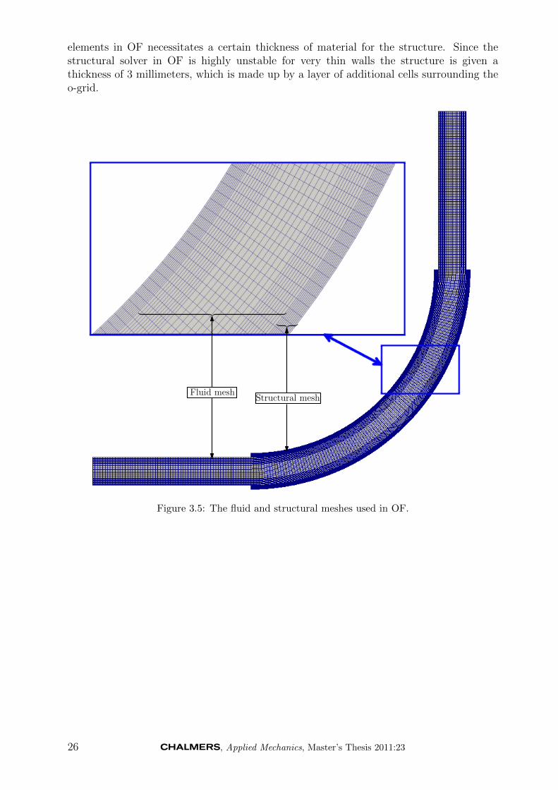
elements in OF necessitates a certain thickness of material for the structure. Since thestructural solver in OF is highly unstable for very thin walls the structure is given athickness of 3 millimeters, which is made up by a layer of additional cells surrounding theo-grid.
Structural meshFluid mesh
︸ ︷︷ ︸︸ ︷︷ ︸
Figure 3.5: The fluid and structural meshes used in OF.
26 , Applied Mechanics, Master’s Thesis 2011:23
Structure
︸ ︷︷ ︸
Fluid domain
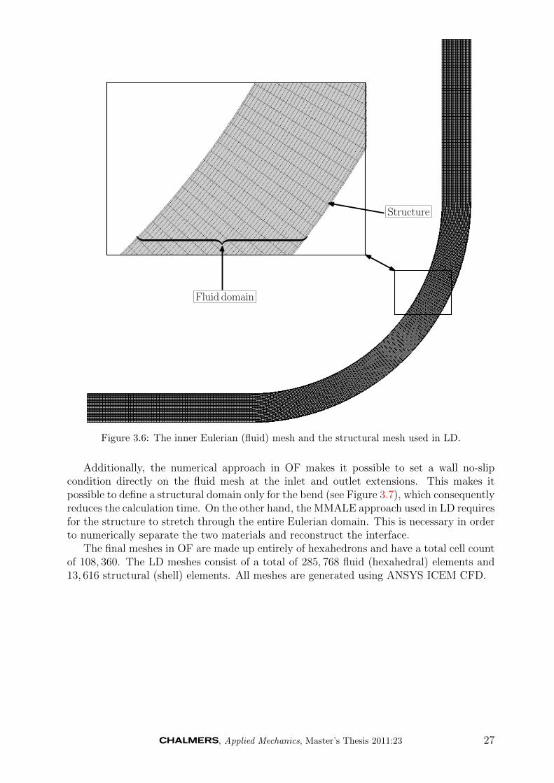
Figure 3.6: The inner Eulerian (fluid) mesh and the structural mesh used in LD.
Additionally, the numerical approach in OF makes it possible to set a wall no-slipcondition directly on the fluid mesh at the inlet and outlet extensions. This makes itpossible to define a structural domain only for the bend (see Figure 3.7), which consequentlyreduces the calculation time. On the other hand, the MMALE approach used in LD requiresfor the structure to stretch through the entire Eulerian domain. This is necessary in orderto numerically separate the two materials and reconstruct the interface.
The final meshes in OF are made up entirely of hexahedrons and have a total cell countof 108, 360. The LD meshes consist of a total of 285, 768 fluid (hexahedral) elements and13, 616 structural (shell) elements. All meshes are generated using ANSYS ICEM CFD.
, Applied Mechanics, Master’s Thesis 2011:23 27

Structural mesh
Fluid mesh
Figure 3.7: The fluid and structural meshes used in OF.
3.3.3 Boundary conditions
The boundary conditions used in the coupled analysis are summed up in Table 3.4. Theinlet boundary has been given two different conditions corresponding to the steady-stateflow and the pulsating flow, respectively.
Table 3.4: Boundary conditions for the coupled analysis.
Software Boundary Type ValueOF Inlet Steady-state velocity 0.5 [m/s]
Periodic velocity 0.5 + 0.5sin(2πft) [m/s]Outlet Mean pressure 0 [Pa]Rigid walls No-slip -Flexible walls Moving wall velocity -Symmetry plane Symmetry -
LD Inlet Steady-state velocity 0.5 [m/s]Periodic velocity 0.5 + 0.5sin(2πft) [m/s]
Outlet Zero traction 0 [N/m2]Rigid walls No-slip -Flexible walls Moving wall velocity -Symmetry plane Symmetry -
28 , Applied Mechanics, Master’s Thesis 2011:23

4 Results
This section covers the results of both the LD and the OF simulations. The simulationsconsist of three groups: firstly the flow solution comparison for a straight rigid pipe,secondly a steady flow through the bent EVG and finally a pulsating flow through thebent EVG. Pressure and velocity distribution at selected locations (see Figure 4.1) as wellas normal forces at the upstream and downstream attachments of the EVG are presented.
r Exit
(a) Straight setup
z
xy
R
Entrance(Upstream attachment)
Exit(Downstream attachment)
r
(b) Bent EVG setup
Figure 4.1: Setup overviews. Pressure and velocity cross-section profiles extractedat ”Entrance” and ”Exit” and normal forces in the coupled analysis extracted atthe upstream and downstream attachments, respectively.
4.1 Validation of laminar flow in a rigid pipe
The data from the straight rigid pipe simulations are sampled at the outlet (or ”Exit”,see Figure 4.1a) cross-section, after a simulated time of 14 seconds. At this point the flowis considered to be fully developed for both solvers. Figure 4.2a shows the cross-sectionvelocity profiles for OF, LD and the analytical solution (see Appendix A). The cross-sectionpressure profiles for OF and LD is plotted in Figure 4.2b.
For the OF simulation the velocity profiles at the outlet show great correspondencewith the analytical solution. The LD simulation seems to give a generally lower velocitythan both OF and the analytical solution, with the exception of the near wall regions (i.e.−0.007 m < r ≤ −0.006 m and 0.006 m ≤ r < 0.007 m).
For the pressure (see Figure 4.2b) some characteristic similarities can be seen betweenthe OF and LD results. However, the pressure at the outlet is lower in LD (though onlywith 0.01 Pa) and shows a more distinct variation of pressure across the pipe. Recall thatthe outlet boundary condition in OF was set to a mean pressure of 0 Pa (see Section 3.2).If assembling the OF pressure in Figure 4.2b, the mean value is not 0 Pa. This is becausethe pressure from the OF simulation is sampled in the cell-centers (i.e. slightly upstreamof the outlet boundary), while the pressure from the LD simulation is sampled directly onthe boundary. This most certainly contributes to the differences in pressure. Moreover, OFsolves for an incompressible flow while LD solves for a compressible fluid with a high bulk
, Applied Mechanics, Master’s Thesis 2011:23 29

modulus. This ought to further contribute to the differences for the pressure calculation.
(a) (b)
Figure 4.2: Plots showing a) velocity profiles of analytical solution, OF simulationand LD simulation and b) pressure profiles of OF simulation and LD simulation.
4.2 Steady flow with FSI
This section presents the results from the simulations using a steady inlet flow boundarycondition with the velocity 0.5 m/s, also taking into account the coupling between the fluidflow and the structure. Figure 4.3 shows comparisons of the cross-sectional velocity andpressure profiles in the symmetry plane. The profiles in Figure 4.3a and Figure 4.3c areextracted at the entrance of the bent EVG (i.e. upstream) and the profiles in Figure 4.3band Figure 4.3d at the exit of the bent EVG (i.e. downstream).
The pressure and velocity profiles from the two softwares are plotted at different times,i.e. t = 2 s for LD and t = 3 s for OF. This is because the LD simulation is run withactivated coupling from t = 0 s, while the coupling in OF is not activated until the flow hasbeen stabilized (e.g. at t = 2 s). The reason for this is the OF solver’s sensitivity to thelarge, transient forces that occur during the development of the flow field. An example ofsuch large force transients, extracted from the LD simulation, can be seen in Figure 4.5a.
Figure 4.4 shows the velocity and pressure fields in the symmetry plane obtained att = 2 s (LD) and t = 3 s (OF), respectively. Figure 4.5c and Figure 4.5d show comparisonsof the normal forces in the upstream and downstream attachments of the bent EVG forthe last 0.5 s of each simulation. As can be seen in Figure 4.5b, the structure in the OFsimulation still experience a ”shock” when the coupling is activated, requiring some timefor the forces to stabilize. However, the magnitudes of these force transients are muchlower than those experienced when activating the coupling already from t = 0 s.
The velocity results for OF and LD (see Figure 4.3) show that the flow is not fullydeveloped before entering the EVG, although a boundary layer is starting to develop. Theboundary layer seems to be further developed in OF than in LD, yielding velocity peaksnear the walls in the LD velocity profile. The reason for the less developed boundary layerin LD is most certainly due to the lower mesh density close to the walls (in comparisonwith the mesh in used in OF).
For both softwares there is a slightly higher velocity towards the leftmost wall (i.e.−0.006 m < r < −0.003 m). This makes sense since the flow is forced by the pressuregradient to ”turn” into the bent EVG, causing the flow to accelerate in this region. Thisis further validated by the pressure profiles in Figure 4.3c. It should be noted that the
30 , Applied Mechanics, Master’s Thesis 2011:23

volume fraction method used in LD (see Section 2.4.2) creates uncertainties regardingthe accurateness of the near wall solution variables. Even though the velocities are ofsimilar magnitude here, the impact of the transition region between the dummy materialand the water can not be disregarded. Furthermore, severe leakage of the water into theouter domain (see Figure 4.6) occur at the inlet boundary as well as local pressure andvelocity peaks. This affects the whole solution and is most probably the reason for the largedifferences between the two solver simulations. Hence, the velocity and pressure profiles forOF and LD, in this section, show less correspondence than the results from the validationof laminar flow in a rigid pipe (see Section 4.1).
The acceleration near the leftmost wall causes the flow to separate when entering theEVG (as clearly indicated in Figure 4.4a and 4.4b). The separation gives rise to a largedecrease in pressure near the innermost wall (see Figure 4.3d and Figure 4.4c - 4.4d).Worth noting is that Figure 4.4a indicates that the flow field is laminar, while Figure 4.4bimplies occurence of turbulence. This partly originates from the use of different meshes,but also from the use of different numerical advection schemes in the two softwares. Thepresence of turbulence in LD is further indicated by the randomness of the velocity profileat the exit of the EVG (see Figure 4.3b).
When further comparing the pressure profiles at the entrance and exit of the EVG(Figure 4.3c and 4.3d) it is evident that the pressure drop through the pipe is larger inLD than in OF. This is, again, validated by the pressure fields in Figure 4.4c and 4.4d.Consequently, the velocities are somewhat higher in the LD simulations, as well as thenormal forces in both the upstream and downstream attachments (see Figure 4.5). Thedifferent coupling methods may contribute to these differences, even though their impactis probably lesser than the two softwares’ ways of solving the flow field. Moreover, in bothsolvers the normal force in the upstream attachment is larger than the downstream normalforce. This is likely to originate from the separation of the flow, yielding a steep pressuregradient in the lower half of the EVG (see e.g. Figure 4.7e).
From the momentum balance calculations, (see Appendix B) a rough estimate is givenfor the upstream and downstream forces where Fx = Fy ≈ 0.03841 N. For OF the upstreamforce fluctuates around 0.0375 N and for LD around 0.0625 N. The downstream force forOF fluctuates around 0.0315 N and LD around 0.0465 N. For both forces, OF is slightlylower than the estimates. This is due to the calculations being performed for a streamtubewhere the streamlines are the same throughout the tube and no losses are considered. Inthe EVG there are frictional losses which reduces the force acting on the structure. For LDthe forces are higher than the estimated forces, in line with previously discussed pressureand leakage related reasons.
, Applied Mechanics, Master’s Thesis 2011:23 31

(a) Entrance velocity profiles (b) Exit velocity profiles
(c) Entrance pressure profiles (d) Exit pressure profiles
Figure 4.3: Plots showing b,c) cross-section velocity profiles and d,e) cross-sectionpressure profiles at the entrance and exit of the bent EVG at t = 2 s (LD) andt = 3 s (OF). Inlet velocity: vz = −0.5 m/s.
32 , Applied Mechanics, Master’s Thesis 2011:23

v [m/s]
0.75
0.6
0.4
0.2
0
(a) Velocity field, OF (t = 3 s)
v [m/s]0.85
0.6
0
0.2
(b) Velocity field, LD (t = 2 s)
p [Pa]
150
120
80
40
0
−1.2
(c) Pressure field, OF (t = 3 s)
p [Pa]200
100
0−10
(d) Pressure field, LD (t = 2 s)
Figure 4.4: a,b) showing velocity fields and c,d) showing pressure fields for OF andLD respectively.
, Applied Mechanics, Master’s Thesis 2011:23 33

(a) Normal forces (LD) (b) Normal forces (OF)
(c) Upstream attachment, last 0.5 s (OF, LD) (d) Downstream attachment, last 0.5 s (OF, LD)
Figure 4.5: Plots a,b) showing force transients and c,d) showing comparisons of nor-mal forces at upstream and downstream attachments for the last 0.5 s, respectively.
(a) Volume fraction t = 0 s (b) Volume fraction t = 0.1 s
Figure 4.6: a) showing initial volume fraction and b) the volume fraction after 0.1s, illustrating the leakage for the steady flow case in LD.
34 , Applied Mechanics, Master’s Thesis 2011:23

4.3 Pulsating flow with FSI
This section presents the results from the simulations using a sinusoidal velocity inlet flowboundary condition. The velocity and pressure results are presented at five different timesand at each time the results are accompanied by a plot showing the current stage of theinlet pulse. Figure 4.7-4.11 show the velocity and pressure fields in the symmetry plane atfive different stages of the inlet pulse. The reason for the different sampling times is againthe OF solver’s sensitivity to the initial force instabilities (see Section 4.2). Figure 4.12 -4.16 show velocity and pressure fields in the symmetry plane at five different stages of thesinusoidal inlet flow condition.
Figure 4.17 shows comparisons of the normal forces in the upstream and downstreamattachments of the EVG. The forces extracted from LD are sampled from t = 0 s, includingthe initial instabilities. This is not the case for OF where the simulation is split into threestages (see Appendix D) due to the solver sensitivity. Hence the normal forces are extractedand plotted only for the last stage, when the forces have been stabilized.
In Figure 4.7 and 4.8 it can be seen that the first 0.5 seconds of the sampled pulses showgreat similarities with the profiles from the simulations using a steady inlet flow condition(see Section 4.2). This is the case also for the last sampling point (see Figure 4.11). As forthe steady flow simulation, the flow characteristics correspond fairly well between the twonumerical solutions, though the magnitudes of pressure and velocity deviate here as well.This is most likely due to the inlet boundary leakage in LD (see Figure 4.18), discussed inSection 4.2.
The greatest differences between the solvers occur when approaching zero inlet velocity,hence between 0.5 s ≤ t ≤ 1 s (see Figure 4.8 - 4.10 and 4.13 - 4.15). The decreasinginlet velocity induces turbulence and since using different grids and advection schemes, theturbulence is not resolved equally. The two advection schemes handle the flux over eachcell differently, leading to a deviation in transport of the solution variables. Since neitherof the grids are fine enough to fully resolve the smallest scales, none of the solutions can.in this sense, be said to be more accurate. However, OF offers a finer mesh close to thestructure, yielding a better resolved boundary layer. Nonetheless, the results within thisinterval must be considered more uncertain.
The normal forces (see Figure 4.17) show fair correspondence with the sinusoidal inletpulse, though the forces are not entirely sinusoidal. What may be noted is the phase shiftof the forces in comparison to the sinusoidal inlet velocity, i.e. the forces reach their criticalvalues before the inlet velocity, but to clarify the reasons for this behavior more extensivesimulations are required. Again, as for the steady state analysis, the forces are consistentlylarger in LD than in OF, and the force at the upstream attachment is generally larger thanthe downstream force in both solvers. Also, the tugging (i.e. positive) forces that arisefrom the stretching of the EVG are slightly larger than the compressive (i.e. negative)forces that arise when the structure retracts from a stretched state.
, Applied Mechanics, Master’s Thesis 2011:23 35
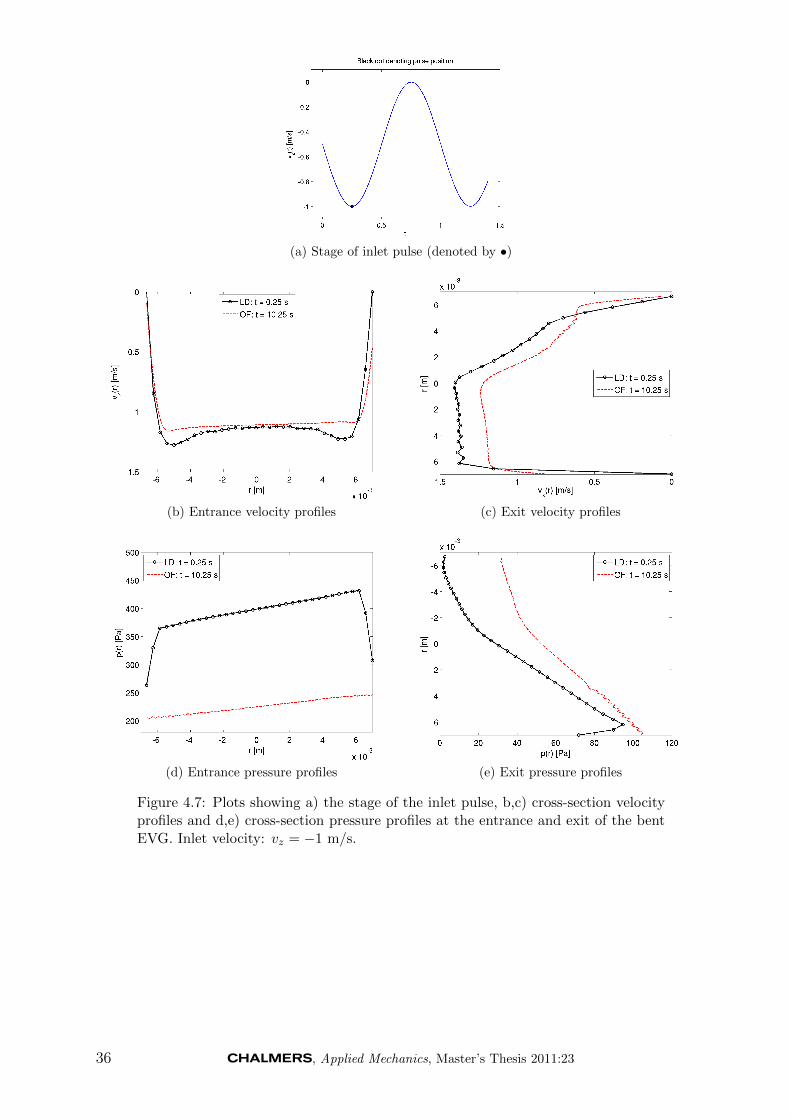
(a) Stage of inlet pulse (denoted by •)
(b) Entrance velocity profiles (c) Exit velocity profiles
(d) Entrance pressure profiles (e) Exit pressure profiles
Figure 4.7: Plots showing a) the stage of the inlet pulse, b,c) cross-section velocityprofiles and d,e) cross-section pressure profiles at the entrance and exit of the bentEVG. Inlet velocity: vz = −1 m/s.
36 , Applied Mechanics, Master’s Thesis 2011:23

(a) Stage of inlet pulse (denoted by •)
(b) Entrance velocity profiles (c) Exit velocity profiles
(d) Entrance pressure profiles (e) Exit pressure profiles
Figure 4.8: Plots showing a) the stage of the inlet pulse, b,c) cross-section velocityprofiles and d,e) cross-section pressure profiles at the entrance and exit of the bentEVG. Inlet velocity: vz = −0.5 m/s.
, Applied Mechanics, Master’s Thesis 2011:23 37

(a) Stage of inlet pulse (denoted by •)
(b) Entrance velocity profiles (c) Exit velocity profiles
(d) Entrance pressure profiles (e) Exit pressure profiles
Figure 4.9: Plots showing a) the stage of the inlet pulse, b,c) cross-section velocityprofiles and d,e) cross-section pressure profiles at the entrance and exit of the bentEVG. Inlet velocity: vz = 0 m/s.
38 , Applied Mechanics, Master’s Thesis 2011:23
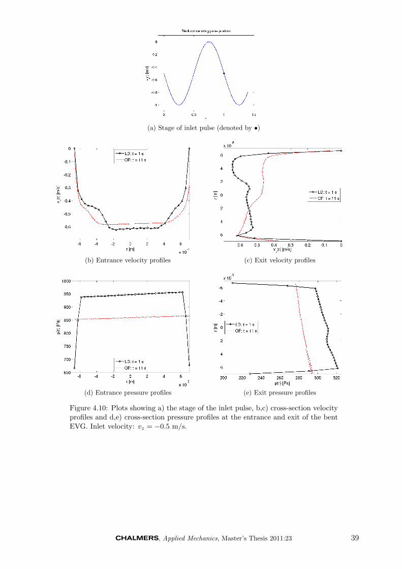
(a) Stage of inlet pulse (denoted by •)
(b) Entrance velocity profiles (c) Exit velocity profiles
(d) Entrance pressure profiles (e) Exit pressure profiles
Figure 4.10: Plots showing a) the stage of the inlet pulse, b,c) cross-section velocityprofiles and d,e) cross-section pressure profiles at the entrance and exit of the bentEVG. Inlet velocity: vz = −0.5 m/s.
, Applied Mechanics, Master’s Thesis 2011:23 39
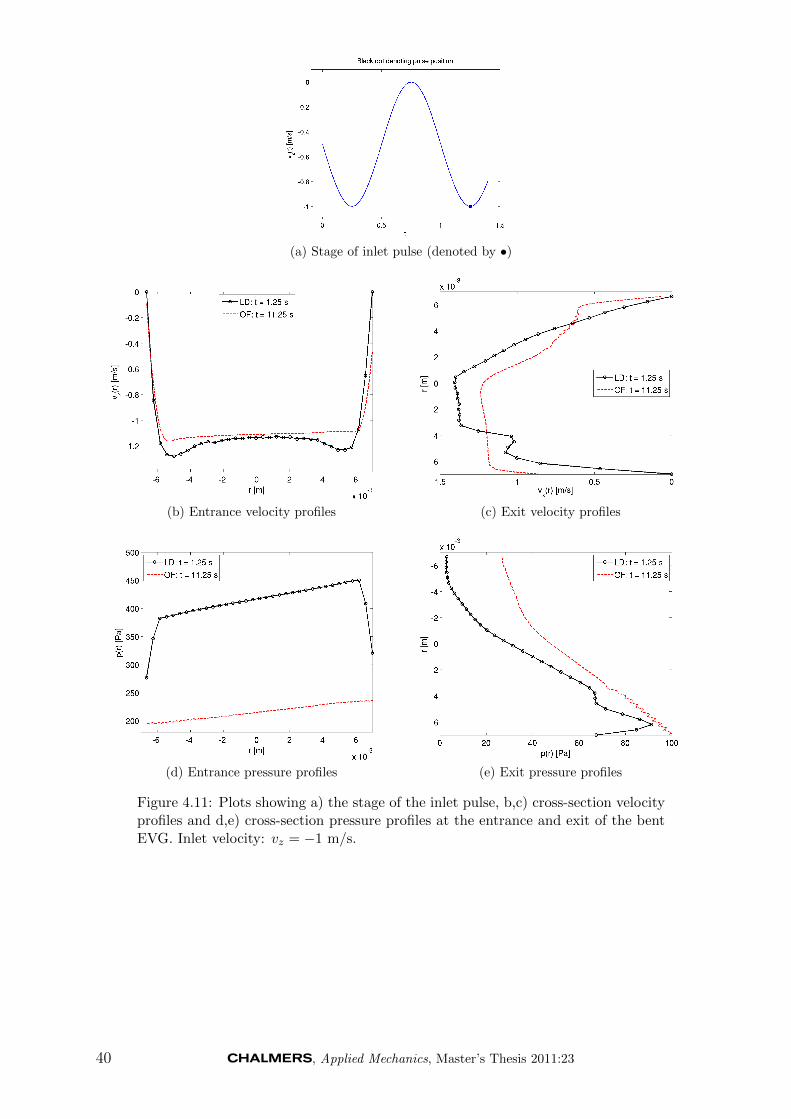
(a) Stage of inlet pulse (denoted by •)
(b) Entrance velocity profiles (c) Exit velocity profiles
(d) Entrance pressure profiles (e) Exit pressure profiles
Figure 4.11: Plots showing a) the stage of the inlet pulse, b,c) cross-section velocityprofiles and d,e) cross-section pressure profiles at the entrance and exit of the bentEVG. Inlet velocity: vz = −1 m/s.
40 , Applied Mechanics, Master’s Thesis 2011:23

(a) Stage of inlet pulse (denoted by •)
Software Upstream force [N] Downstream force [N]OF 0.1298 0.1058LD 0.2286 0.1756
(b) Normal forces at current stage
v [m/s]
1.5
0.8
0.4
0
1.2
0.8
0.4
(c) Velocity field, OF
v [m/s]1.5
0
0.3
1.2
0.9
0.6
(d) Velocity field, LD
400
p [Pa]
300
200
100
0−12
(e) Pressure field, OF
p [Pa]600
−30
200
400
(f) Pressure field, LD
Figure 4.12: a) shows the stage of the inlet pulse, b) shows the normal forces at thecurrent stage, c,d) show velocity fields from OF and LD, respectively, and e,f) showpressure fields from OF and LD, respectively.
, Applied Mechanics, Master’s Thesis 2011:23 41

(a) Stage of inlet pulse (denoted by •)
Software Upstream force [N] Downstream force [N]OF -0.0644 -0.0721LD -0.0060 -0.0213
(b) Normal forces at current stage
v [m/s]
1
0.8
0.6
0.4
0.2
0
(c) Velocity field, OF
v [m/s]1
0
0.2
0.8
0.6
0.4
(d) Velocity field, LD
p [Pa]
60
−200
−400
−600
−800
−900
(e) Pressure field, OF
p [Pa]50
−1000
−600
−300
(f) Pressure field, LD
Figure 4.13: a) shows the stage of the inlet pulse, b) shows the normal forces at thecurrent stage, c,d) show velocity fields from OF and LD, respectively, and e,f) showpressure fields from OF and LD, respectively.
42 , Applied Mechanics, Master’s Thesis 2011:23

(a) Stage of inlet pulse (denoted by •)
Software Upstream force [N] Downstream force [N]OF -0.0420 -0.0452LD -0.0019 -3.6300e-04
(b) Normal forces at current stage
v [m/s]
0.5
0.4
0.3
0.2
0.1
0
(c) Velocity fields, OF
v [m/s]0.5
0
0.1
0.4
0.3
0.2
(d) Velocity fields, LD
−40
−20
0
10
p [Pa]
(e) Pressure fields, OF
p [Pa]30
−60
−30
0
(f) Pressure fields, LD
Figure 4.14: a) shows the stage of the inlet pulse, b) shows the normal forces at thecurrent stage, c,d) show velocity fields from OF and LD, respectively, and e,f) showpressure fields from OF and LD, respectively.
, Applied Mechanics, Master’s Thesis 2011:23 43
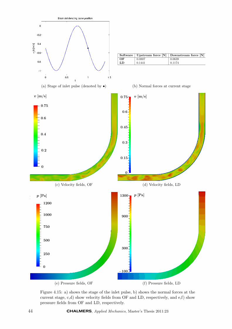
(a) Stage of inlet pulse (denoted by •)
Software Upstream force [N] Downstream force [N]OF 0.0807 0.0639LD 0.1441 0.1174
(b) Normal forces at current stage
0.6
0.4
0.2
0
v [m/s]
0.75
(c) Velocity fields, OF
v [m/s]0.75
0
0.15
0.6
0.45
0.3
(d) Velocity fields, LD
p [Pa]
1200
1000
750
500
250
0
(e) Pressure fields, OF
p [Pa]1300
−100
300
900
(f) Pressure fields, LD
Figure 4.15: a) shows the stage of the inlet pulse, b) shows the normal forces at thecurrent stage, c,d) show velocity fields from OF and LD, respectively, and e,f) showpressure fields from OF and LD, respectively.
44 , Applied Mechanics, Master’s Thesis 2011:23
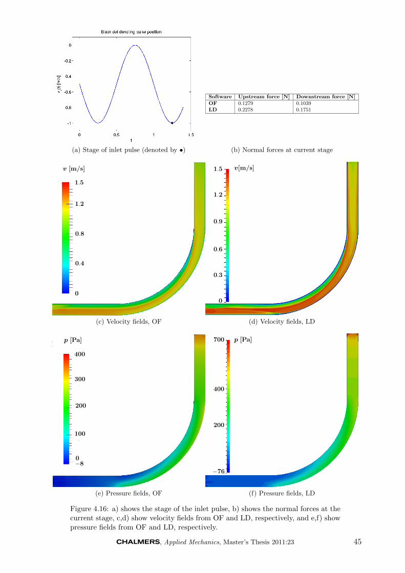
(a) Stage of inlet pulse (denoted by •)
Software Upstream force [N] Downstream force [N]OF 0.1279 0.1039LD 0.2278 0.1751
(b) Normal forces at current stage
v [m/s]
1.5
1.2
0.8
0.4
0
(c) Velocity fields, OF
v[m/s]1.5
0
0.3
1.2
0.9
0.6
(d) Velocity fields, LD
p [Pa]
400
300
200
100
0−8
(e) Pressure fields, OF
p [Pa]700
−76
200
400
(f) Pressure fields, LD
Figure 4.16: a) shows the stage of the inlet pulse, b) shows the normal forces at thecurrent stage, c,d) show velocity fields from OF and LD, respectively, and e,f) showpressure fields from OF and LD, respectively.
, Applied Mechanics, Master’s Thesis 2011:23 45

(a) Upstream normal forces (b) Downstream normal forces
Figure 4.17: Comparisons of upstream and downstream attachment normal forcesfor a sinusoidal inlet flow boundary condition.
(a) Volume fraction t = 0 s (b) Volume fraction t = 0.1 s
Figure 4.18: a) showing initial volume fraction and b) the volume fraction after 0.1s, illustrating the leakage for the pulsating flow case in LD.
46 , Applied Mechanics, Master’s Thesis 2011:23

5 Conclusions
As stated in Section 1.2, one of the main goals of this project is to investigate the possibil-ity of using FSI simulations to assess the forces causing stent graft migration. Prior work,such as the ones performed by Li and Kleinstreuer [1, 24] and Molony et al. [25], demon-strate rather successful results from FSI simulations applying an FE approach and a mixedFE/FV approach, respectively. The force estimations in [1, 24] are the most relevant forcomparison, since they are extracted at the bifurcating region of the EVG, and are in linewith the forces estimated in the work by Malina et al. [5]. However, the forces extractedin the present study are inferior to the ones obtained by Li and Kleinstreuer. These differ-ences most certainly originate from the dissimilarities in numerical approaches, boundaryconditions, geometry and fluid medium. Furthermore, the forces are not extracted at thesame locations.
Based on the work done by Li and Kleinstreuer [1, 24] and Molony et al. [25], theconclusion is that FSI simulations are realizable and possible to perform in such mannerthat a fair evaluation of the forces causing stent graft migration is achieved. However,this project does only offer results from further simplified simulations of the problem (seeSection 1.4 and 1.5), also using different softwares than in prior studies. Nonetheless, theresults show good promise of utilizing both LD and OF for more complex studies similarto those previously discussed. With this said, there are still several aspects that need to beimproved and further tested to reach a more satisfactory level of complexity that furtherresembles an in vivo5 stent graft. Examples of such improvements are a more aggressive(in terms of a steeper gradient), and hence more realistic, inlet pulse and a non-zero gaugepressure.
An additional purpose of this project is to compare the numerical approaches used inLD and OF. This is done by studying the velocity, pressure and resulting forces. Overall,LD gives higher magnitudes for these variables and this is mainly believed to be causedby the leakage of material and peaks in pressure and velocity at the inlet. Hence thecredibility of these results is arguable. It is, however, likely that LD performs well witha finer tuned setup. For example, the constraint based coupling algorithm used in thepresent setup performs poorly for the rigid parts (i.e. the inlet and outlet) [26], though apenalty based coupling algorithm would instead require an extensive process of trial anderror to establish important coupling parameters.
The approach used in OF does not suffer from any problems related to material mix-ing, since the different materials are separated into two different meshes. Instead, thelargest difficulties are related to the remeshing procedure that follows a deformation ofthe structural mesh (and hence the displacement of the fluid-structure interface). Theremeshing requirement leads to a sensitivity to large distortions, yielding an unstable andtime consuming solution procedure (see Appendix D.2). Another drawback with the FVformulation is the requirement of volume elements, making it difficult to simulate very thinstructures. On a more positive note, OF offers full insight to the source code, providingpossibilities to investigate the implementation of the mathematical formulations and toimplement modifications of the solver.
As a final remark, the authors believe that further testing and tuning of the modulesused in this project can be of great interest, with the long-term objective of providing alter-natives to the softwares used in prior studies. Since the setups used in this project partlylack complexity, it should be clearly stated that the forces extracted are not to be consid-ered as guiding values in terms of in vivo stent graft migration. Nonetheless, the studyprovides helpful information about the functionalities of the two numerical approaches.
5i.e. within a living organism
, Applied Mechanics, Master’s Thesis 2011:23 47
6 Recommendations
As mentioned in Section 5, several improvements are to be considered for future studies.First and foremost, it is recommended to apply a more aggressive and realistic inlet pulse,similar to the ones used by e.g. Li and Kleinstreuer [1, 6, 24] and Molony et al. [25].Additionally, a more representative gauge pressure is recommended in order to regard alarger inflation of the EVG, possibly contributing to larger forces. To gain further confi-dence in future studies it is recommended to perform parallel experimental and numericalstudies, enabling comparisons of the results. Experimental studies may also be used toensure proper material properties.
Furthermore, parametric studies of alternate geometries (e.g. EVG diameter and cur-vature) and alternate heart rates, possibly corresponding to patients suffering from hyper-tension6, can be of great interest. In the long run it may also be meaningful to model anon-newtonian blood flow rather than water, since it impacts the flow behavior and hencethe interaction with the EVG. Last, but not least, performing longer simulations wouldgive the possibility to further investigate phenomenas such as the phase shift of forces inthe pulsating case.
6i.e. elevated blood pressure
48 , Applied Mechanics, Master’s Thesis 2011:23

References
[1] Li, Z. & Kleinstreuer, C., “Analysis of biomechanical factors affecting stent-graftmigration in an abdominal aortic aneurysm model,” Journal of Biomechanics, vol. 39,2006.
[2] Basford, J. R., “The Law of Laplace and Its Relevance to Contemporary Medicineand Rehabilitation,” Archives of Physical Medicine and Rehabilitation, vol. 83, no. 8,2002.
[3] Resch, T., Ivancev, K., Brunkwall, J., Nyman, U., Malina, M. & Lindblad, B.,“Distal Migration of Stent-Grafts after Endovascular Repair of Abdominal AorticAneurysms,” Journal of Vascular and Interventional Radiology, vol. 10, no. 3, 1999.
[4] Zarins, C. K., Bloch, D. A., Crabtree, T., Matsumoto, A. H., White, R. A. & Foga-rty, T. J., “Stent graft migration after endovascular aneurysm repair: Importance ofproximal fixation,” Journal of Vascular Surgery, vol. 38, 2003.
[5] Malina, M., Lindblad, B., Ivancev, K., Lindh, M., Malina, H. & Brunkwall, J., “En-dovascular AAA Exclusion: Will Stents With Hooks and Barbs Prevent Stent-GraftMigration?,” Journal of Endovascular Surgery, vol. 5, no. 4, 1998.
[6] Li, Z. & Kleinstreuer, C., “Fluid-Structure Interaction Effects on Sac-Blood Pres-sure and Wall Stress in a Stented Aneurysm,” Journal of Biomechanical Engineering,vol. 127, no. 4, 2005.
[7] Ponthot, J.P & Belytschko, T., “Arbitrary Lagrangian-Eulerian formulation forelement-free Galerkin method,” Computer Methods in Applied Mechanics and En-gineering, vol. 152, 1998.
[8] Yeh, I., Chai, L. & Saha, N., “Application of ALE to airbag deployment simulation,”Int. J. Vehicle Safety, vol. 1, no. 4, 2006.
[9] Toll, S. & Ekh, M., Lecture notes, “TME075 - Mechanics of solids & fluids. Part I:Fundamentals,” August 2009.
[10] White, F. M., Fluid Mechanics. McGraw-Hill, 6th ed., 2008.
[11] Ottosen, N. & Petersson, H., Introduction to the Finite Element Method. PrenticeHall, 1st ed., 1992.
[12] Versteeg, H. K. & Malalasekera, W., An Introduction to Computational Fluid Dynam-ics - The Finite Volume Method. Prentice Hall, 2nd ed., 2007.
[13] Livermore Software Technology Corporation, LS-DYNA Theory Manual, 2006.
[14] Olovsson, L., Lecture notes, “LS-DYNA, Training class in ALE and fluid-structureinteraction,” May 2006.
[15] Kurose, S. & Takahashi, S., “Constraint-Based Simulation of Interactions BetweenFluids and Unconstrained Rigid Bodies,” in Proceedings of the 2009 Spring Conferenceon Computer Graphics, SCCG ’09, ACM, 2009.
[16] Amsden, A. A., Ruppel, H. M., & Hirt, C. W., “SALE: A Simplified ALE ComputerProgram for Fluid Flow at All Speeds,” Los Alamos Scientific Laboratory, 1980. LA-8095.
, Applied Mechanics, Master’s Thesis 2011:23 49
[17] Benson, D. J., “Momentum Advection on a Staggered Mesh,” Journal of Computa-tional Physics, vol. 100, no. 1, 1992.
[18] Tukovic, Z. & Jasak, H., “Updated Lagrangian Finite Volume Solver for large defor-mation dynamic response of elastic body,” Transactions of FAMENA, vol. 31, 2007.
[19] Jasak, H & Weller, H. G., “Application of the finite volume method and unstruc-tured meshes to linear elasticity,” International Journal for Numerical Methods inEngineering, vol. 48, 2000.
[20] OpenCFD Limited, OpenFOAM User Guide, July 2009. version 1.6.
[21] Morststedt, S-E. & Hellsten, G., Data och Diagram - Energi- och kemitekniska tabeller.Liber, 7th ed., 2008.
[22] Cutnell, J. D. & Johnson, K. W., Physics. Wiley, 4th ed., 1998.
[23] Graebel, W. P., Engineering Fluid Mechanics. Taylor & Francis, 1st ed., 2001.
[24] Li, Z. & Kleinstreuer, C., “Blood flow and structure interactions in a stented abdom-inal aortic aneurysm model,” Medical Engineering & Physics, vol. 27, no. 5, 2005.
[25] Molony, D. S., Kavanagh, E. G., Madhavan, P., Walsh, M. T. & McGloughlin, T.M., “A Computational Study of the Magnitude and Direction of Migration Forcesin Patient-specific Abdominal Aortic Aneurysm Stent-Grafts,” European Journal ofVascular and Endovascular Surgery, vol. 40, no. 3, 2010.
[26] Livermore Software Technology Corporation, LS-DYNA, Keyword User’s Manual,2003.
50 , Applied Mechanics, Master’s Thesis 2011:23
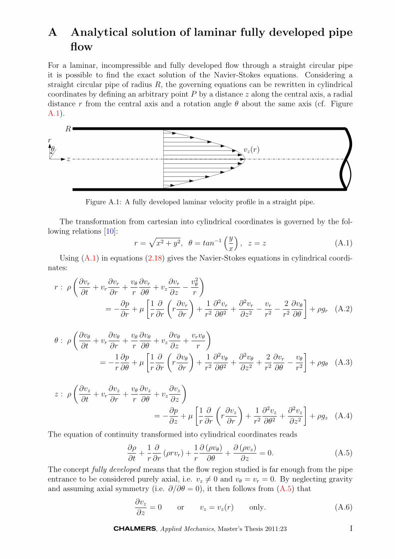
A Analytical solution of laminar fully developed pipe
flow
For a laminar, incompressible and fully developed flow through a straight circular pipeit is possible to find the exact solution of the Navier-Stokes equations. Considering astraight circular pipe of radius R, the governing equations can be rewritten in cylindricalcoordinates by defining an arbitrary point P by a distance z along the central axis, a radialdistance r from the central axis and a rotation angle θ about the same axis (cf. FigureA.1).
r
zθ
R
vz(r)
Figure A.1: A fully developed laminar velocity profile in a straight pipe.
The transformation from cartesian into cylindrical coordinates is governed by the fol-lowing relations [10]:
r =√x2 + y2, θ = tan−1
(yx
), z = z (A.1)
Using (A.1) in equations (2.18) gives the Navier-Stokes equations in cylindrical coordi-nates:
r : ρ
(∂vr∂t
+ vr∂vr∂r
+vθr
∂vr∂θ
+ vz∂vr∂z− v2θ
r
)
= −∂p∂r
+ µ
[1
r
∂
∂r
(r∂vr∂r
)+
1
r2∂2vr∂θ2
+∂2vr∂z2− vrr2− 2
r2∂vθ∂θ
]+ ρgr (A.2)
θ : ρ
(∂vθ∂t
+ vr∂vθ∂r
+vθr
∂vθ∂θ
+ vz∂vθ∂z
+vrvθr
)
= −1
r
∂p
∂θ+ µ
[1
r
∂
∂r
(r∂vθ∂r
)+
1
r2∂2vθ∂θ2
+∂2vθ∂z2
+2
r2∂vr∂θ− vθr2
]+ ρgθ (A.3)
z : ρ
(∂vz∂t
+ vr∂vz∂r
+vθr
∂vz∂θ
+ vz∂vz∂z
)
= −∂p∂z
+ µ
[1
r
∂
∂r
(r∂vz∂r
)+
1
r2∂2vz∂θ2
+∂2vz∂z2
]+ ρgz (A.4)
The equation of continuity transformed into cylindrical coordinates reads
∂ρ
∂t+
1
r
∂
∂r(ρrvr) +
1
r
∂ (ρvθ)
∂θ+∂ (ρvz)
∂z= 0. (A.5)
The concept fully developed means that the flow region studied is far enough from the pipeentrance to be considered purely axial, i.e. vz 6= 0 and vθ = vr = 0. By neglecting gravityand assuming axial symmetry (i.e. ∂/∂θ = 0), it then follows from (A.5) that
∂vz∂z
= 0 or vz = vz(r) only. (A.6)
, Applied Mechanics, Master’s Thesis 2011:23 I
This holds provided that the flow is steady and incompressible. Similarly, the r-momentumequation, eq. (A.2), simplifies to
∂p
∂r= 0 or p = p(z) only. (A.7)
Consequently, equation (A.4) reduces to
− ∂p
∂z+µ
r
∂
∂r
(r∂vz∂r
)= 0. (A.8)
Equation (A.8) is linear and may be integrated twice yielding the result
vz =∂p
∂z
r2
4µ+ C1ln (r) + C2 (A.9)
where C1 and C2 are constants. The boundary conditions are no-slip at the wall andmaximum velocity at the centerline (cf. Figure A.1):
r = 0;∂vz∂r
= 0
r = R; vz = 0.(A.10)
The constants in equation (A.9) can then be obtained as
C1 = 0 and C2 = −∂p∂z
(R2
4µ
). (A.11)
The final expression for laminar fully developed pipe flow is now obtained as
vz(r) = −∂p∂z
(1
4µ
)(R2 − r2
). (A.12)
II , Applied Mechanics, Master’s Thesis 2011:23

B Simple force estimation for a steady flow
In order to establish confidence in the extracted forces, a simple calculation is performedto estimate the force needed to balance the change in momentum of an inviscid fluid as itis deflected in a bent streamtube (see Figure B.1a). Consider a fixed CV of a streamtubewith the same steady, uniform inlet flow boundary condition and geometry as for the EVG(see Figure B.1b). The diameter d = 0.014 m yields a circular area of A = π · (d/2)2 m2.Together with the density of water ρ = 998 kg/m3 and the velocity
VIn = [0 0 − 0.5], VOut = [0.5 0 0] and |V| = |VIn| = |VOut| = 0.5 m/s
yields a mass flow of
m = mIn = mOut = ρA|V| ≈ 0.07682 kg/s.
For a one dimensional cross section, where V and ρ is uniform over the area and with theconservation of mass, the linear momentum equation reads [10]
F =d
dt
(∫
CV
Vρ dV
)+ (mV)Out − (mV)In (B.1)
The volume integral vanishes for a steady flow, such that the force becomes
F = m(VOut −VIn). (B.2)
This yields the x and y force components
Fx = Fz ≈ 0.03841 N.
mVIn
mVOut z
x y
F = m(VOut −VIn)
(a)
VOut
d = 0.014 m
VIn
m = constant
(b)
Figure B.1: a) shows a vector diagram for force calculation and b) a streamtube insteady flow.
, Applied Mechanics, Master’s Thesis 2011:23 III
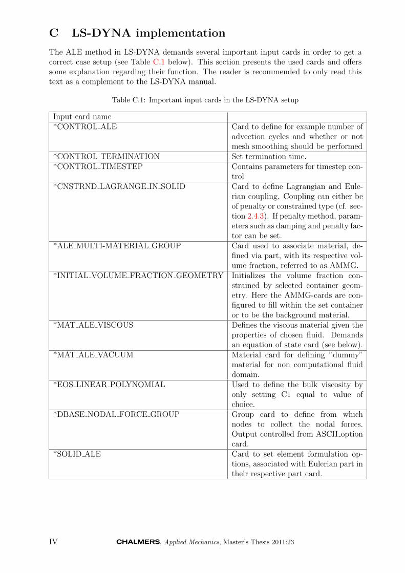
C LS-DYNA implementation
The ALE method in LS-DYNA demands several important input cards in order to get acorrect case setup (see Table C.1 below). This section presents the used cards and offerssome explanation regarding their function. The reader is recommended to only read thistext as a complement to the LS-DYNA manual.
Table C.1: Important input cards in the LS-DYNA setup
Input card name*CONTROL ALE Card to define for example number of
advection cycles and whether or notmesh smoothing should be performed
*CONTROL TERMINATION Set termination time.*CONTROL TIMESTEP Contains parameters for timestep con-
trol*CNSTRND LAGRANGE IN SOLID Card to define Lagrangian and Eule-
rian coupling. Coupling can either beof penalty or constrained type (cf. sec-tion 2.4.3). If penalty method, param-eters such as damping and penalty fac-tor can be set.
*ALE MULTI-MATERIAL GROUP Card used to associate material, de-fined via part, with its respective vol-ume fraction, referred to as AMMG.
*INITIAL VOLUME FRACTION GEOMETRY Initializes the volume fraction con-strained by selected container geom-etry. Here the AMMG-cards are con-figured to fill within the set containeror to be the background material.
*MAT ALE VISCOUS Defines the viscous material given theproperties of chosen fluid. Demandsan equation of state card (see below).
*MAT ALE VACUUM Material card for defining ”dummy”material for non computational fluiddomain.
*EOS LINEAR POLYNOMIAL Used to define the bulk viscosity byonly setting C1 equal to value ofchoice.
*DBASE NODAL FORCE GROUP Group card to define from whichnodes to collect the nodal forces.Output controlled from ASCII optioncard.
*SOLID ALE Card to set element formulation op-tions, associated with Eulerian part intheir respective part card.
IV , Applied Mechanics, Master’s Thesis 2011:23

D OpenFOAM implementation
As mentioned in Section 2.5 the simulation in OpenFOAM was performed using an ex-tended version of the icoFsiFoam solver. This section covers the case setup, as well as thesteps which the FSI simulations are divided into.
D.1 Case setup
The file structure for cases run with this solver differs somewhat from the typical standard(single-phase) cases in OpenFOAM. First off, the case is divided into two separate sub-folders; one for the fluid simulation and one for the structural simulation. These foldersare, from now on, referred to as fluid and solid, respectively. The file structures for thefluid and solid directories look as follows:
fluid solid
|-- 0 |-- 0
| |-- motionU | ‘-- DU
| |-- p |-- constant
| |-- solid -> ../../solid/0 | |-- polyMesh
| ‘-- U | | |-- boundary
|-- constant | | |-- cellZones
| |-- couplingProperties | | |-- faces
| |-- dynamicMeshDict | | |-- faceZones
| |-- polyMesh | | |-- neighbour
| | |-- boundary | | |-- owner
| | |-- cellZones | | |-- points
| | |-- faces | | |-- pointZones
| | |-- faceZones | | |-- sets
| | |-- neighbour | | | ‘-- interfaceSolidZone
| | |-- owner | | ‘-- zoneToPatchName
| | |-- points | ‘-- rheologyProperties
| | |-- pointZones |-- system
| | |-- sets | |-- controlDict
| | | ‘-- interfaceFluidZone | |-- decomposeParDict
| | ‘-- zoneToPatchName | |-- fvSchemes
| |-- solid -> ../../solid/constant | |-- fvSolution
| ‘-- transportProperties
|-- system
| |-- controlDict
| |-- decomposeParDict
| |-- fvSchemes
| |-- fvSolution
| |-- sampleDict
| |-- solid -> ../../solid/system
| ‘-- tetFemSolution
The initial and boundary conditions are defined in the 0 directories located directlyunder the fluid and solid directories. The pressure and velocity conditions for the fluidare defined in p and U, respectively, while the displacement increment condition for the
, Applied Mechanics, Master’s Thesis 2011:23 V

structure is defined in DU. The file motionU contains the conditions for the deforming meshmotion, which is a requirement for the FSI analysis. The motion of the mesh at thefluid-structure interface has to be implemented as a Dirichlet boundary condition for thefluid velocity. This is done using movingWallVelocity as the boundary condition in U
at the interface.The constant subdirectories (i.e. polyMesh, transportProperties andrheologyProperties) contain information about the meshes and the material properties(e.g. density, viscosity, Young’s modulus etc.) for the different phases. Most of thesettings governing the fluid-structure interaction are defined in couplingProperties andthe settings for the solution of the mesh motion are defined in dynamicMeshDict. Thesystem directories are where the solution procedure is setup. Settings such as end time,time step and time interval for output to be written are all defined in the file controlDict.The files fvSchemes and fvSolution contain information about which differencing schemesto use and settings for convergence tolerances. The decomposeParDicts describe how thecomputational domains should be decomposed for cases that are to be run in parallel. Thebranches of the type solid -> are, so-called, soft links linking together the settings forthe fluid phase with the solid phase. These links are necessary in order for the solver toget input to the solution of both the fluid and structural equation systems.
The fluid-structure interface is defined after the fluid and solid meshes have both beencreated. This is done by typing
setSet -case fluid
faceSet <fluidInterfaceName> new patchToFace <fluidInterfacePatchName>
quit
setsToZones -case fluid -noFlipMap
setSet -case solid
faceSet <solidInterfaceName> new patchToFace <solidInterfacePatchName>
quit
setsToZones -case solid -noFlipMap
when standing in the main case folder. The interface could then be used for the settingsin the file couplingProperties located in the subdirectory fluid/constant. This filecontained the residual tolerance for the FSI.
Since the straight pipe in the first study (see Section 3.2) are to be given rigid walls,the coupling implementation of the solver has to be turned off, making it solve only forthe flow. This is done by setting
fsi no;
in couplingProperties.
VI , Applied Mechanics, Master’s Thesis 2011:23

D.2 Simulation steps
Due to convergence problems, the OF FSI simulations have to be split into three stages.They are
1. Perform an initial, uncoupled steady flow simulation. Run until stabilized.
2. Perform an uncoupled, pulsating flow simulation. Run for a few pulses.
3. Perform a coupled, pulsating flow simulation.
i) Calculate normal forces in EVG attachments.
Thanks to this procedure, large initial instabilites (which causes the solution to diverge)can be avoided.
, Applied Mechanics, Master’s Thesis 2011:23 VII