Seediscussions,stats,andauthorprofilesforthispublicationat:https://www.researchgate.net/publication/306034496

FluidandParticleCoarseningofDragForceforDiscrete-ParcelApproach

Article·August2016

DOI:10.1016/j.ces.2016.08.014

READS

3

4authors:

AliOzel

PrincetonUniversity

18PUBLICATIONS43CITATIONS

SEEPROFILE

JariKolehmainen

PrincetonUniversity

10PUBLICATIONS8CITATIONS

SEEPROFILE

StefanRadl

GrazUniversityofTechnology

89PUBLICATIONS368CITATIONS

SEEPROFILE

SankaranSundaresan

PrincetonUniversity

226PUBLICATIONS5,237CITATIONS

SEEPROFILE

Allin-textreferencesunderlinedinbluearelinkedtopublicationsonResearchGate,

lettingyouaccessandreadthemimmediately.

Availablefrom:AliOzel

Retrievedon:12August2016

Author’s Accepted Manuscript

Fluid and Particle Coarsening of Drag Force forDiscrete-Parcel Approach

Ali Ozel, Jari Kolehmainen, Stefan Radl, SankaranSundaresan

PII: S0009-2509(16)30436-5DOI: http://dx.doi.org/10.1016/j.ces.2016.08.014Reference: CES13111

To appear in: Chemical Engineering Science

Received date: 9 June 2016Revised date: 2 August 2016Accepted date: 8 August 2016

Cite this article as: Ali Ozel, Jari Kolehmainen, Stefan Radl and SankaranSundaresan, Fluid and Particle Coarsening of Drag Force for Discrete-ParcelA p p r o a c h , Chemical Engineering Science,http://dx.doi.org/10.1016/j.ces.2016.08.014

This is a PDF file of an unedited manuscript that has been accepted forpublication. As a service to our customers we are providing this early version ofthe manuscript. The manuscript will undergo copyediting, typesetting, andreview of the resulting galley proof before it is published in its final citable form.Please note that during the production process errors may be discovered whichcould affect the content, and all legal disclaimers that apply to the journal pertain.

www.elsevier.com/locate/ces

Fluid and Particle Coarsening of Drag Force for Discrete-Parcel Approach

Ali Ozela,∗, Jari Kolehmainena, Stefan Radlb, Sankaran Sundaresana

aDepartment of Chemical and Biological Engineering, Princeton University, Princeton, NJ 08544, USAbInstitute of Process and Particle Engineering, Graz University of Technology, Inffeldgasse 13/III, 8010 Graz, Austria

Abstract

Fine-grid Euler-Lagrange simulations of gas-fluidization of uniformly sized particles have been performed in

three-dimensional periodic domains. Snapshots obtained from these simulations have been systematically

coarse-grained to extract filter size dependent corrections to the drag law that should be employed in coarse

Euler-Euler (EE) simulations. Correction to the drag law that should be employed in Coarse Multi-Phase

Particle-in-Cell (MP-PIC) model simulations is examined through a two-step process: separating the coars-

ening of the fluid and particle phases. It is found that the drag correction is almost entirely due to the

coarsening of the fluid cells, with particle coarsening having only a weak effect. It is shown that drag cor-

rection for coarse EE and MP-PIC simulations are comparable. As a result, coarse drag models developed

for EE simulations can serve as a good estimate for corrections in MP-PIC simulations, and vice versa.

Keywords: MP-PIC, parcel approach, fluid coarsening, particle coarsening, drag force, filtered two-fluid

model

1. Introduction

Industrial-scale gas-particle flow systems exhibit flow structures which span a wide range of spatial and

temporal scales; bubble-like voids of varying sizes rising at different velocities form in dense beds, while

dynamic clusters of different shapes and sizes are found in dilute flows. These meso-scale structures affect

the macro-scale flow patterns, which impacts the performance of fluidized bed chemical reactors. This5

multi-scale nature of flow complicates analysis and scale-up of these devices. Coarse simulation methods

that can reproduce reliably the macro-scale flow structures in these devices have been a topic of much

research (Agrawal et al., 2001; Wang and Li, 2007; Igci and Sundaresan, 2011a; Parmentier et al., 2012; Ozel

et al., 2013; Milioli et al., 2013; Schneiderbauer and Pirker, 2014).

Industrial-scale fluidized bed simulations can be classified into two groups: (1) Eulerian-Eulerian simula-10

tions based on two-fluid model (TFM) approach (Gidaspow, 1994; Syamlal et al., 1993; Balzer et al., 1998)

and (2) Eulerian-Lagrangian simulations based on multiphase particle-in-cell method (MP-PIC) (Snider,

2001; Snider and Banerjee, 2010; Snider et al., 2011).

∗Corresponding authorEmail address: aozel@princeton.edu (Ali Ozel)

Preprint submitted to Chemical Engineering Science August 8, 2016

In TFM simulations of gas-particle flows, one must postulate models for the interphase interaction force

and the effective stresses in the two phases. The particle phase stress model is either postulated in an ad-hoc15

manner (Jackson, 2000) or calculated using the kinetic theory for granular flow (KTGF) and a fluctuating

granular energy equation (e.g., see Gidaspow (1994); Koch and Sangani (1999); Balzer et al. (1998); Lun

et al. (1984); Ding and Gidaspow (1990)). In MP-PIC simulations, the continuum averaged equations of

motion for the gas phase are solved on an Eulerian grid, while representative particles, commonly referred

to as parcels representing a plurality of real particles, are tracked in a Lagrangian manner. As in TFM, this20

approach requires a model for the interphase interaction force. Furthermore, collisions between parcels are

not tracked; but are captured indirectly through a postulated particle phase stress (Snider, 2001; O’Rourke

and Snider, 2012; O’Rourke et al., 2009; Snider, 2007). The Discrete Particle Model (DPM) proposed by

Patankar and Joseph (2001) seeks to circumvent the need for postulating a stress model in the parcel-based

simulation by treating the parcels as effectively larger particles and tracking collisions between the parcels.25

Collision tracking is generally very expensive and hence DPM-based approach has not gained much attraction

for industrial scale device simulations.

It is generally accepted that meso-scale structures affect the macro-scale flow characteristics. As a result,

one must either resolve the meso-scale structures or recognize their consequences in some indirect manner.

Li and Kwauk (1994) recognized that the presence of clusters leads to a significant decrease in the effective30

fluid-particle drag and introduced the energy-minimization-multi-scale (EMMS) method, which has been

refined and extended since then (Wang and Li, 2007; Wang et al., 2008). The meso-scale patterns, which

the EMMS method sought to average over, can be observed in TFM simulations when fine numerical grids

are employed (e.g., see Agrawal et al. (2001); Ozel et al. (2013)). MP-PIC simulations with fine grids reveal

these structures as well; indeed, with fine Eulerian grids, both TFM and MP-PIC approaches reveal similar35

meso-scale structures (Benyahia and Sundaresan, 2012).

When fine numerical grids are employed, all the particles are tracked in an Euler-Lagrange simulation

(i.e. parcel size is one), and all the collisions are resolved, one obtains the so-called Computational Fluid

Dynamics-Discrete Element Method (CFD-DEM). This method has served as a vehicle to probe meso-

scale flow structures (Ye et al., 2004; Capecelatro and Desjardins, 2013; Capecelatro et al., 2014a,b; Radl40

and Sundaresan, 2014; Salikov et al., 2015) and the consequences of complex particle-particle interactions

(Kobayashi et al., 2013; Girardi et al., 2016; Kolehmainen et al., 2016; Gu et al., 2016; Fries et al., 2013). The

CFD-DEM approach is computationally expensive and is limited to small-scale flows, as one can realistically

track no more than a few million particles.

The use of fine grids is not practical for industrial scale flow problems (Sundaresan, 2000), necessitating45

the use of coarse (fluid) grids in both TFM and MP-PIC methods and treatment of particle-particle interac-

tions through a stress model. Such coarse simulations require coarse-grained constitutive models to account

for the consequences of unresolved flow structures.

A procedure for systematically coarse-graining the TFM to obtain the so-called filtered TFM has already

2

been presented in the literature (Igci et al., 2008; Parmentier et al., 2012; Ozel et al., 2013; Milioli et al.,50

2013; Schneiderbauer and Pirker, 2014; O’Brien, 2014; Fox, 2014) The filtered TFM contains additional

residual correlations (such as filtered solid stress and drag force), which must be modeled. It is now known

that the filtered drag force depends on filter size and can be significantly smaller than that predicted by

the original drag force models; this correction to the drag law is the most important difference between the

original and filtered TFMs (Igci and Sundaresan, 2011a; Parmentier et al., 2012; Ozel et al., 2013; Milioli55

et al., 2013; Schneiderbauer and Pirker, 2014). Ozarkar et al. (2015) show that the sub-grid contribution of

particle phase stress has a slight effect on the macroscopic flow predictions such as time-average pressure and

velocity profiles, as well as the solids inventory in a dense fluidized bed. However, in the context of dilute

dispersed flows, Moreau et al. (2009) point out that the trace of sub-grid contribution of particle stresses

has a dispersive characteristic and it is crucial to obtaining a better prediction of particle segregation.60

Coarse-graining CFD-DEM simulation results is beginning to gain attention only recently (Radl and

Sundaresan, 2014; Capecelatro et al., 2014b,a, 2016b,a), motivated by the need for closures to be used in

coarser models. These authors have simulated fluidized suspensions in fully/wall-bounded periodic domains

and analyzed the snapshots. Radl and Sundaresan (2014) examined how the drag law should be modified

when one coarsens the fluid grid size, while continuing to simulate through DEM the motion of all the65

particles in the simulation domain. Such coarsening, referred to as fluid coarsening, revealed the need for

a filter size dependent effective drag law, which is conceptually similar to what is known in the context of

TFMs. These authors speculated that the drag law may also depend on parcel size in both MP-PIC and

DPM based approaches. However, they did not perform a systematic particle coarsening to check whether

their speculation is correct, or considered the derivation of drag closures for Euler-Euler-based models from70

their CFD-DEM data. In contrast, Capecelatro et al. (2016b,a) propose closures for Reynolds-averaged

Euler-Euler-based models for gas-particle flows from CFD-DEM predictions. It should be remarked that

there is a long history of seeking closures for effective stresses and fluid turbulence particle interactions in

Euler-Euler models from Euler-Lagrange simulation results (e.g., see Simonin (1991); Vance et al. (2006);

Fede and Simonin (2006); Kaufmann et al. (2008)); however, these studies typically do not seek correction75

to drag.

The present study is concerned with a systematic coarsening of computational data generated through

detailed simulations to develop effective drag force models for filtered Euler-Euler and MP-PIC approaches.

Although it would be desirable to generate the required computational data through fully-resolved Euler-

Lagrange simulations, where the motion of the particles are followed using Newton’s equations and the80

interstitial fluid flow is completely resolved through direct numerical simulation (Koch and Ladd, 1997;

Derksen and Sundaresan, 2007; Rubinstein et al., 2016; Tenneti et al., 2010, 2011; Vincent et al., 2014;

Ozel et al., 2016), such simulations are very expensive and flows involving only a few thousand particles

can realistically be simulated through this approach. In contrast, one can readily perform CFD-DEM

simulations, which requires a microscopic drag law as an input, in larger domains containing millions of85

3

particles (Capecelatro et al., 2014a). Hence, this approach is more suitable for developing filtered drag laws

that are applicable for very coarse simulations. Work aimed at developing such coarse drag laws by filtering

CFD-DEM simulation results are beginning to emerge (Radl and Sundaresan, 2014; Girardi et al., 2016;

Capecelatro et al., 2016b,a).

One can also generate computational data through finely resolved Euler-Euler simulations, but these90

simulations require particle phase stress model as well. Continuum particle-phase stress models that account

for complex particle-particle interactions, such as van der Waals, capillary or electrostatic interactions, are

still under development. In contrast, these interactions are quite easily included in CFD-DEM simulations,

and therefore we pursue CFD-DEM simulations to generate the computational database needed for coarse

model development.95

By filtering the CFD-DEM results, one can generate four types of results: (1) coarse-grained drag that

can be used with filtered Euler-Euler simulations, (2) coarse-grained drag model that can be used with coarse

MP-PIC and coarse CFD-DPM simulations, (3) continuum particle phase stress model that can be used in

well resolved Euler-Euler simulations, and (4) coarse-grained stress models that can be used with filtered

Euler-Euler and coarse MP-PIC simulations. In the present study, we are concerned with items 1 and 2 in100

the above list.

The general approach to extract such drag models is follows. In the CFD-DEM simulations used to

generate the snapshots, a user-specified grid size is employed to solve the averaged equation for the gas

phase, which is 3dp in the examples presented in this paper, where dp denotes particle diameter. In order

to develop effective drag law for filtered Euler-Euler approach, we first map the Lagrangian variables from105

particle locations onto the Eulerian field and then compute the filtered Eulerian drag force for different

filter sizes by following the procedure already outlined in the literature (Igci and Sundaresan, 2011a; Ozel

et al., 2013). Drag model for Euler-Lagrange simulations can be coarsened in two ways: (1) One seeks

modifications to the drag force model when only coarsening the grid size used for solving the fluid phase

equations, while continuing to solve for the motion of all the particles as in the original fine-grid simulation.110

This is the fluid coarsening referred to earlier. (2) One seeks a modified drag law that applies when one

further coarsens the problem by following the motion of only a subset of the particles (along with the fluid

coarsening). This is the particle coarsening referred to earlier. This is illustrated in Figure 1 schematically.

In general, particle coarsening should be accompanied by fluid coarsening as well, since one must have a fair

number of representative particles inside each fluid cell to get reasonable statistics.115

In the present study we address the following questions:

• What is the relative importance of fluid and particle coarsening on the extent of correction to the drag

law for coarse Euler-Lagrange simulations?

• When applying the drag law, the drag force is evaluated in the Eulerian cell (i.e., in Euler-Euler

based models) and at the particle (parcel) location in the other (when seeking to perform well resolved120

simulations, researchers currently use the same drag law (e.g., Wen and Yu (1966)) in both Euler-Euler

4

(a) (b) (c)

Fluid coarsening Particle coarseningdp

dparcelΔ Δf Δf

dp

Figure 1: Schematic illustration showing fine-grid Euler-Lagrange simulations (panel (a); colors indicate the local particleconcentration) to obtain constitutive relationships for fluid-coarsened (panel (b)), and coarse-grid MP-PIC simulations withparcels representative of many particles (panel (c), dparcel refers to the diameter of a parcel).

simulations, researchers currently use the same drag law (e.g., Wen and Yu (1966)) in both Euler-Euler

and Euler-Lagrange simulations.) How does this difference affect the fashion in which the effective drag

law changes with extent of coarsening for the Euler-Euler and Euler-Lagrange simulations?

To answer these questions, we coarse-grain the same set of computationally generated snapshots to125

extract effective drag corrections applicable to both coarse Euler-Euler and Euler-Lagrange simulations. We

will demonstrate that fluid coarsening is mostly responsible for the correction to the drag law and that for

small filter sizes there is a small difference in the coarsened drag laws for the Euler-Euler and Euler-Lagrange

simulations. This difference becomes smaller as one increases the extent of fluid and particle coarsening. As

a result, one can, to a good approximation, avail the drag corrections developed in the literature for coarse130

Euler-Euler simulations in coarse Euler-Lagrange simulations as well.

This paper is organized as follows. We present the mathematical modeling and flow configuration, which

is a 3D fully periodic square prism, in §2. Fluid and particle coarsening procedures are described in §3. In

§4, the coarse-grained results are presented. The principal results are summarized in section, §5.

2. Mathematical Modeling and Flow Configuration135

In the Discrete Element Method (DEM) (Cundall and Strack, 1979), particles are tracked by solving

Newton’s equations of motion:

midvi

dt=

∑

j

(fnc,ij + f t

c,ij) + fg→p,i +mig (1)

Iidωi

dt=

∑

j

T t,ij (2)

5

Figure 1: Schematic illustration showing fine-grid Euler-Lagrange simulations (panel (a); colors indicate the local particleconcentration) to obtain constitutive relationships for fluid-coarsened (panel (b)), and coarse-grid MP-PIC simulations withparcels representative of many particles (panel (c), dparcel refers to the diameter of a parcel).

and Euler-Lagrange simulations.) How does this difference affect the fashion in which the effective drag

law changes with extent of coarsening for the Euler-Euler and Euler-Lagrange simulations?

To answer these questions, we coarse-grain the same set of computationally generated snapshots to

extract effective drag corrections applicable to both coarse Euler-Euler and Euler-Lagrange simulations. We125

will demonstrate that fluid coarsening is mostly responsible for the correction to the drag law and that for

small filter sizes there is a small difference in the coarsened drag laws for the Euler-Euler and Euler-Lagrange

simulations. This difference becomes smaller as one increases the extent of fluid and particle coarsening. As

a result, one can, to a good approximation, avail the drag corrections developed in the literature for coarse

Euler-Euler simulations in coarse Euler-Lagrange simulations as well.130

This paper is organized as follows. We present the mathematical modeling and flow configuration, which

is a 3D fully periodic square prism, in §2. Fluid and particle coarsening procedures are described in §3. In

§4, the coarse-grained results are presented. The principal results are summarized in section, §5.

2. Mathematical Modeling and Flow Configuration

In the Discrete Element Method (DEM) (Cundall and Strack, 1979), particles are tracked by solving

Newton’s equations of motion:

midvidt

=∑

j

(fnc,ij + f tc,ij) + fg→p,i +mig (1)

Iidωidt

=∑

j

T t,ij (2)

In the equations, particle i is spherical and has mass mi, moment of inertia Ii, translational and angular135

velocities vi and ωi. The forces acting on the particle i are: fnc,ij and f tc,ij which are the normal and

5

tangential contact forces between two particles i and j; fg→p,i which is the total interaction force on the

particle i due to surrounding gas (explained further below), and mig is the gravitational force. The torque

acting on particle i due to particle j is T t,ij . T t,ij = Rij × f tc,ij , where Rij is the vector from the center of

particle i to the contact point.140

The particle contact forces fnc,ij and f tc,ij are calculated by the following Johnson and Johnson (1987);

Di Renzo and Di Maio (2004):

fnc,ij =4

3Y ∗√r∗δ3/2

n nij + 2

√5

6β√Snm∗v

nij , (3)

f tc,ij =

−8G∗

√r∗δntij + 2

√56β√Stm∗vtij for

∣∣f tc,ij∣∣ < µs

∣∣fnc,ij∣∣

−µs∣∣fnc,ij

∣∣ tij|tij | for

∣∣f tc,ij∣∣ ≥ µs

∣∣fnc,ij∣∣ ,

(4)

where

1

Y ∗=

1− ν2i

Yi+

1− ν2j

Yj,

1

r∗=

1

ri+

1

rj, (5)

β =ln(e)√

ln2(e) + π2, Sn = 2Y ∗

√r∗δn, (6)

1

G∗=

2(2 + νi)(1− νi)Yi

+2(2 + νj)(1− νj)

Yj, St = 8G∗

√r∗δn. (7)

The subscripts i, j denote spherical particle i or j, and the superscript ∗ denotes the effective particle

property of those two particles. The effective particle mass m∗ is calculated as m∗ = mimj/(mi + mj); δn

is normal overlap distance; nij represents the unit normal vector pointing from particle j to particle i; vnij

represents the normal velocity of particle j relative to particle i; tij represents the tangential displacement

obtained from the integration of the relative tangential velocity during the contact, vtij ; and µs is the particle145

sliding friction coefficient. Here, Y is Young’s modulus, G is shear modulus, ν is Poisson’s ratio, and r is

particle radius.

The fluid phase is modeled by solving the following conservation of mass and momentum equations in

terms of the locally averaged variables over a computational cell:

∂

∂t(1− φ) + ∇ · [(1− φ)ug] = 0, (8)

ρg(1− φ)

(∂ug∂t

+ ug ·∇ug)

= −∇pg + ∇ · τ g + Φd + ρg(1− φ)g. (9)

Here, ρg is the density of the gas which is assumed to be constant, φ is the solid volume fraction, ug is the150

gas velocity, pg is the gas phase pressure, τ g is the gas phase deviatoric stress tensor. The total gas-particle

interaction force per unit volume of the mixture −Φd, exerted on the particles by the gas, is composed of a

generalized buoyancy force due to the slowly-varying (in space) local-average gas phase stress (−pgI + τ g)

and the force due to the rapidly varying flow (in space) field around the particles.

6

In finite volume method based computations employed in our simulations, Φd in any computational cell

is related to fg→p,i of all the particles in that cell as Φd = −∑cell

i fg→p,i

V where V is the volume of the

computational cell. On a per particle basis, the total interaction force on the particle by the gas can be

written as fg→p,i = −Vp,i∇pg|x=xp,i+ Vp,i∇ · τ g|x=xp,i

+ fd,i , where Vp,i is the particle volume and fd,i

is the drag force calculated by the Wen and Yu (1966) drag law. The gas phase deviatoric stress tensor

contribution is relatively insignificant in fg→p,i for modeling gas-fluidized beds of particles (Agrawal et al.,

2001) and hence ignored. The total interaction force is mapped on the Eulerian grid using a mollification

kernel ξ characterized by a smoothing length equal to the mesh spacing ∆ by following Pepiot and Desjardins

(2012). The kernel function ξ is defined by

ξ(L) =

14L4 − 5

8L2 + 115192 , if L ≤ 0.5

− 16L4 + 5

6L3 − 54L2 + 5

24L+ 5596 , if 0.5 < L ≤ 1.5

(2.5−L)4

24 , if 1.5 < L ≤ 2.5

0, otherwise

(10)

where L = d/∆ and d is the distance from the particle position xp,i to face center coordinate x. The155

total force is mapped over the 27 nearest cells around the particle location. Alternatively, the mapping

of Lagrangian properties on the Eulerian mesh could be performed by using trilinear interpolation (Snider

et al., 1998; Patankar and Joseph, 2001). Subscript i indicates that quantities are per particle, and that fluid

phase properties have been interpolated at the particle position, |x=xp,i . The fluid variables at the particle

position are computed by a linear interpolation using the distance weightings L.160

The gas phase equations are solved using an OpenFOAM-based Computational Fluid Dynamics solver

(OpenFOAM, 2013), while the particle phase DEM equations are evolved via the LIGGGHTS platform

(Kloss et al., 2011). The two phases are coupled via CFDEMcoupling (Kloss et al., 2012; Goniva et al.,

2012).

We performed simulations in periodic domains in which one can examine the flow dynamics without wall-165

induced restrictions. To drive the flow in this periodic domain, we decompose the pressure term pg in Eq. (9)

into two components as follows: pg(x, t) = p′′g (x, t) − ρ||g||(z − zo). Here, p′′g is the computed gas pressure

that obeys the periodic boundary condition and ρ||g||(z−zo) represents the mean vertical pressure drop due

to the total mass of a two-phase mixture; ρ is the domain-averaged mixture density; z is the coordinate in

the direction that is opposite of gravity and zo is a reference elevation.170

Although we will present our results in dimensionless form, it is useful to present typical dimensional

quantities to demonstrate that the simulations have been done for gas-particle systems of practical interest.

With this in mind, we present the simulation parameters in both dimensional and dimensionless forms in

Table 1. Simulations were performed for three different domain-averaged solid volume fractions < φ >:

0.02, 0.1, 0.2 and 0.3, and three different particle sizes. The simulations were run for a sufficiently long175

7

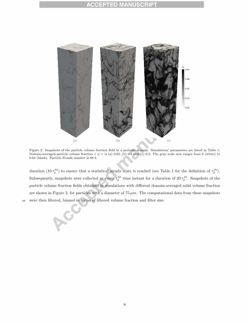
(a) (b)

0.16

0.32

0.48

0.00

0.64φ

(c)

Figure 2: Snapshots of the particle volume fraction field in a periodic domain. Simulations’ parameters are listed in Table 1.Domain-averaged particle volume fraction < φ > is (a) 0.02, (b) 0.1 and (c) 0.3. The gray scale axis ranges from 0 (white) to0.64 (black). Particle Froude number is 88.4.

Table 1. Simulations were performed for three different domain-averaged solid volume fractions < φ >:175

0.02, 0.1, 0.2 and 0.3, and three different particle sizes. The simulations were run for a sufficiently long

duration (10 τStp ) to ensure that a statistical steady state is reached (see Table 1 for the definition of τSt

p ).

Subsequently, snapshots were collected at every τStp time instant for a duration of 20 τSt

p . Snapshots of the

particle volume fraction fields obtained in simulations with different domain-averaged solid volume fraction

are shown in Figure 2, for particles with a diameter of 75µm. The computational data from these snapshots180

were then filtered, binned in terms of filtered volume fraction and filter size.

8

Figure 2: Snapshots of the particle volume fraction field in a periodic domain. Simulations’ parameters are listed in Table 1.Domain-averaged particle volume fraction < φ > is (a) 0.02, (b) 0.1 and (c) 0.3. The gray scale axis ranges from 0 (white) to0.64 (black). Particle Froude number is 88.4.

duration (10 τStp ) to ensure that a statistical steady state is reached (see Table 1 for the definition of τStp ).

Subsequently, snapshots were collected at every τStp time instant for a duration of 20 τStp . Snapshots of the

particle volume fraction fields obtained in simulations with different domain-averaged solid volume fraction

are shown in Figure 2, for particles with a diameter of 75µm. The computational data from these snapshots

were then filtered, binned in terms of filtered volume fraction and filter size.180

8

Table 1: Computational domain and simulations parameters.

Simulations Parameters Value

Particle diameter; dp [µm] 75 / 150 / 300

Domain size; (dp × dp × dp) 240× 240× 960

Grid size; (dp × dp × dp) 3× 3× 3

Acceleration due to gravity; g [m/s2] 9.81

Particle density; ρp [kg/m3] 1500

Young’s modulus; Y [Pa] 106

Poisson’s ratio; ν 0.42

Restitution coefficient; e 0.9

Particle-particle friction coefficient; µp 0.5

Gas density; ρg [kg/m3] 1.3

Gas viscosity; µg [Pa · s] 1.8×10−5

Stokes relaxation time; τStp =ρpdp

2

18µg[s] 0.026 / 0.104 / 0.416

Terminal velocity of a single particle

based on Wen and Yu (1966) drag law; vt [m/s] 0.255 / 1.022 / 4.080

Domain-averaged solid volume fraction < φ > 0.02 / 0.1 / 0.2† / 0.3‡

Number of particles 2.1× 106/10.5× 106/21× 106/31.5× 106

Froude number based on

terminal velocity; Frp = vt2/(||g||dp) 88.4 / 709.8 / 5656.3

† The simulations with the domain-averaged solid volume fraction of 0.2 were performed only for particles with

diameters of 150µm and 300µm.

‡ The simulation with the domain-averaged solid volume fraction of 0.3 was performed only for particles with a

diameter of 75µm.

3. Coarsening Procedure

3.1. Fluid Coarsening

The correction to the drag force needed for Euler-Lagrange simulations with coarser fluid grids was

deduced by filtering the results from highly resolved simulations. Firstly, the particle volume fraction, gas

pressure and gas velocity were filtered using various filter sizes ∆f around each computational node. The

filtered solid volume fraction is computed by

φ(x, t) =

∫ ∫ ∫φ(r, t)G(r− x)dr (11)

9

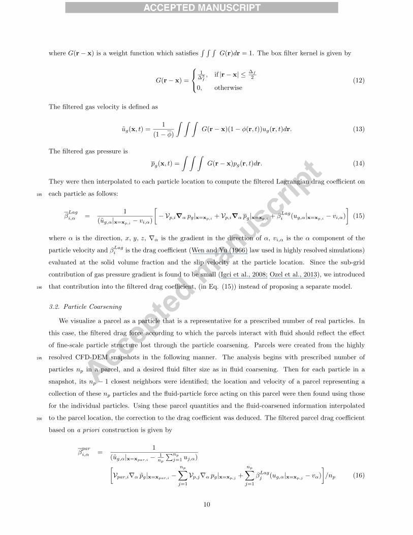
where G(r− x) is a weight function which satisfies∫ ∫ ∫

G(r)dr = 1. The box filter kernel is given by

G(r− x) =

1∆3

f, if |r− x| ≤ ∆f

2

0, otherwise(12)

The filtered gas velocity is defined as

ug(x, t) =1

(1− φ)

∫ ∫ ∫G(r− x)(1− φ(r, t))ug(r, t)dr. (13)

The filtered gas pressure is

pg(x, t) =

∫ ∫ ∫G(r− x)pg(r, t)dr. (14)

They were then interpolated to each particle location to compute the filtered Lagrangian drag coefficient on

each particle as follows:185

βLag

i,α =1

(ug,α|x=xp,i− vi,α)

[− Vp,i∇α pg|x=xp,i

+ Vp,i∇α pg|x=xp,i+ βLagi (ug,α|x=xp,i

− vi,α)

](15)

where α is the direction, x, y, z, ∇α is the gradient in the direction of α, vi,α is the α component of the

particle velocity and βLagi is the drag coefficient (Wen and Yu (1966) law used in highly resolved simulations)

evaluated at the solid volume fraction and the slip velocity at the particle location. Since the sub-grid

contribution of gas pressure gradient is found to be small (Igci et al., 2008; Ozel et al., 2013), we introduced

that contribution into the filtered drag coefficient, (in Eq. (15)) instead of proposing a separate model.190

3.2. Particle Coarsening

We visualize a parcel as a particle that is a representative for a prescribed number of real particles. In

this case, the filtered drag force according to which the parcels interact with fluid should reflect the effect

of fine-scale particle structure lost through the particle coarsening. Parcels were created from the highly

resolved CFD-DEM snapshots in the following manner. The analysis begins with prescribed number of195

particles np in a parcel, and a desired fluid filter size as in fluid coarsening. Then for each particle in a

snapshot, its np − 1 closest neighbors were identified; the location and velocity of a parcel representing a

collection of these np particles and the fluid-particle force acting on this parcel were then found using those

for the individual particles. Using these parcel quantities and the fluid-coarsened information interpolated

to the parcel location, the correction to the drag coefficient was deduced. The filtered parcel drag coefficient200

based on a priori construction is given by

βpar

i,α =1

(ug,α|x=xpar,i − 1np

∑np

j=1 uj,α)

[Vpar,i∇α pg|x=xpar,i −

np∑

j=1

Vp,j∇α pg|x=xp,j +

np∑

j=1

βLagj (ug,α|x=xp,j − vα)

]/np (16)

10

where |x=xpar,i denotes the filtered gas variables at the parcel location and Vpar,i is the parcel volume that

equals to the total volume of the particles participating in a parcel, npVp. It is then divided by np (i.e.

expressed on a per particle basis) so that one can compare βpar

and βLag

.

3.3. Euler-Euler filtering205

One of the goals of this study is to assess the difference between filtered Euler-Euler and Euler-Lagrange

results. We can use this analysis to argue if one can use Euler-Euler filtered drag model in MP-PIC simula-

tions or vice-versa. To perform Euler-Euler filtering, we first mapped the solid velocity us to the cell centers

in a priori manner by using the mollification kernel given in Eq. (10). Then, we computed the filtered

Eulerian drag coefficient as:210

βEul

α =1

(ug,α − us,α)

[φ∇α pg − φ∇α pg + βEul(ug,α − us,α)

]

where us,α is the filtered solid velocity at the cell center and given by

us(x, t) =1

φ

∫ ∫ ∫G(r− x)φ(r, t)us(r, t)dr (17)

and βEuli is the Eulerian drag coefficient (Wen and Yu (1966)).

4. Filtering Results

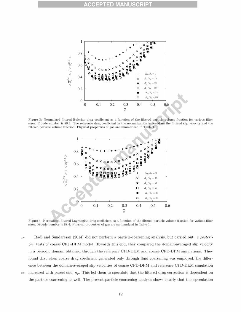
The filtered Eulerian drag coefficient as a function of the filtered particle volume fraction for various filter

sizes is shown in Figure 3. It reveals a significant reduction in filtered drag coefficient even when the filter

size is only 9 dp. This means that when we perform TFM simulations, a sub-grid correction to the drag law215

is necessary even with grid sizes as small as 9 dp. This could be one reason why TFM simulations show grid

size sensitivity even with very fine grids , and in case a filtered drag model is not used.

The filtered Lagrangian drag coefficient as a function of the filtered particle volume fraction for various

filter sizes is shown in Figure 4. Here, only fluid coarsening has been performed, as was done by Radl and

Sundaresan (2014); the present analysis considers much larger filter sizes. The strong effect of fluid filter220

size seen in Figure 4.

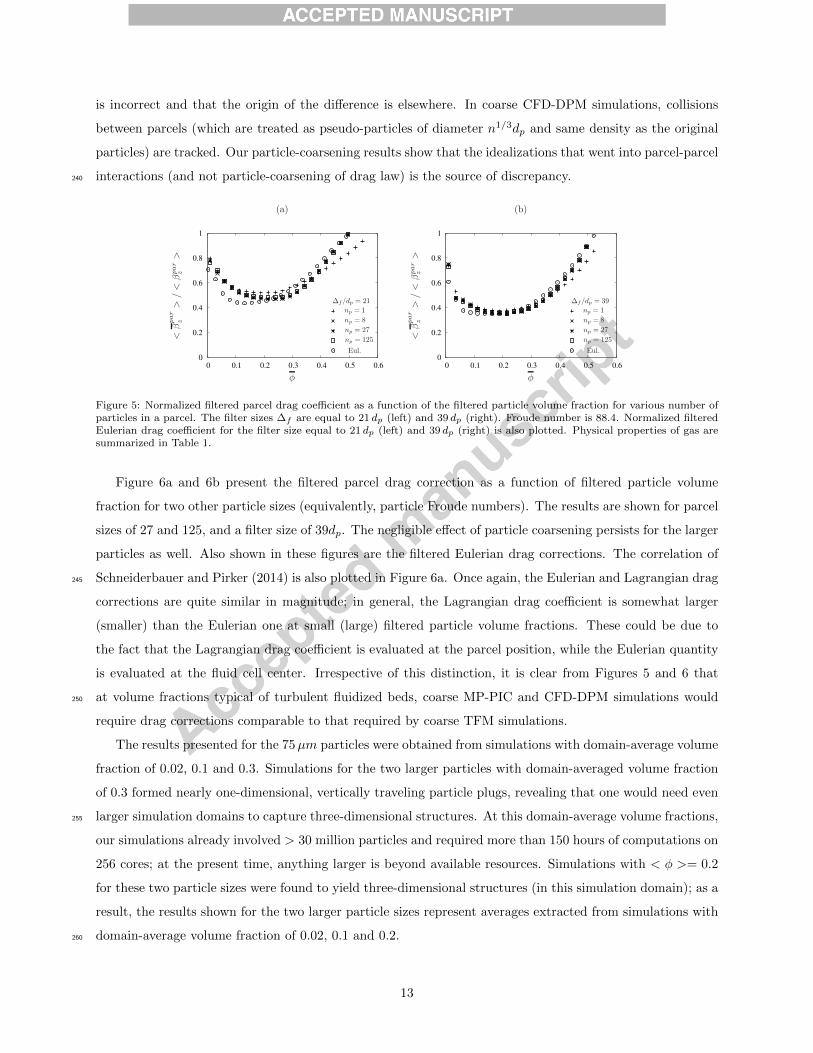
The outcome of particle coarsening is presented in Figure 5a and 5b for particles with Frp = 88.4. The

filtered parcel drag correction is presented in these figures as a function of filtered particle volume fraction

for various parcel sizes and two different filter sizes. The figures also include the filtered Eulerian drag

correction. The filtered parcel drag correction changes slightly upon increasing the parcel size from 1 to 8225

particles, but any further increase produces little change. The filtered parcel drag correction for parcel sizes

of 8 or larger is close to the filtered Eulerian drag correction at most filtered particle volume fraction. It is

readily apparent from Figures 4 and 6 that correction to the filtered drag coefficient comes largely from fluid

coarsening.

11

0

0.2

0.4

0.6

0.8

1

0 0.1 0.2 0.3 0.4 0.5 0.6

φ

<βEul

z>

/<

βEul

z>

∆f/dp = 9

∆f/dp = 15

∆f/dp = 21

∆f/dp = 27

∆f/dp = 33

∆f/dp = 39

Figure 3: Normalized filtered Eulerian drag coefficient as a function of the filtered particle volume fraction for various filtersizes. Froude number is 88.4. The reference drag coefficient in the normalization is based on the filtered slip velocity and thefiltered particle volume fraction. Physical properties of gas are summarized in Table 1.

0

0.2

0.4

0.6

0.8

1

0 0.1 0.2 0.3 0.4 0.5 0.6

φ

<βLag

z>

/<

βLag

z>

∆f/dp = 9

∆f/dp = 15

∆f/dp = 21

∆f/dp = 27

∆f/dp = 33

∆f/dp = 39

Figure 4: Normalized filtered Lagrangian drag coefficient as a function of the filtered particle volume fraction for various filtersizes. Froude number is 88.4. Physical properties of gas are summarized in Table 1.

Radl and Sundaresan (2014) did not perform a particle-coarsening analysis, but carried out a posteri-

ori tests of coarse CFD-DPM model. Towards this end, they compared the domain-averaged slip velocity

in a periodic domain obtained through the reference CFD-DEM and coarse CFD-DPM simulations. They

found that when coarse drag coefficient generated only through fluid coarsening was employed, the differ-

12

Figure 3: Normalized filtered Eulerian drag coefficient as a function of the filtered particle volume fraction for various filtersizes. Froude number is 88.4. The reference drag coefficient in the normalization is based on the filtered slip velocity and thefiltered particle volume fraction. Physical properties of gas are summarized in Table 1.

0

0.2

0.4

0.6

0.8

1

0 0.1 0.2 0.3 0.4 0.5 0.6

φ

<βEul

z>

/<

βEul

z>

∆f/dp = 9

∆f/dp = 15

∆f/dp = 21

∆f/dp = 27

∆f/dp = 33

∆f/dp = 39

Figure 3: Normalized filtered Eulerian drag coefficient as a function of the filtered particle volume fraction for various filtersizes. Froude number is 88.4. The reference drag coefficient in the normalization is based on the filtered slip velocity and thefiltered particle volume fraction. Physical properties of gas are summarized in Table 1.

0

0.2

0.4

0.6

0.8

1

0 0.1 0.2 0.3 0.4 0.5 0.6

φ

<βLag

z>

/<

βLag

z>

∆f/dp = 9

∆f/dp = 15

∆f/dp = 21

∆f/dp = 27

∆f/dp = 33

∆f/dp = 39

Figure 4: Normalized filtered Lagrangian drag coefficient as a function of the filtered particle volume fraction for various filtersizes. Froude number is 88.4. Physical properties of gas are summarized in Table 1.

Radl and Sundaresan (2014) did not perform a particle-coarsening analysis, but carried out a posteri-

ori tests of coarse CFD-DPM model. Towards this end, they compared the domain-averaged slip velocity

in a periodic domain obtained through the reference CFD-DEM and coarse CFD-DPM simulations. They

found that when coarse drag coefficient generated only through fluid coarsening was employed, the differ-

12

Figure 4: Normalized filtered Lagrangian drag coefficient as a function of the filtered particle volume fraction for various filtersizes. Froude number is 88.4. Physical properties of gas are summarized in Table 1.

Radl and Sundaresan (2014) did not perform a particle-coarsening analysis, but carried out a posteri-230

ori tests of coarse CFD-DPM model. Towards this end, they compared the domain-averaged slip velocity

in a periodic domain obtained through the reference CFD-DEM and coarse CFD-DPM simulations. They

found that when coarse drag coefficient generated only through fluid coarsening was employed, the differ-

ence between the domain-averaged slip velocities of coarse CFD-DPM and reference CFD-DEM simulation

increased with parcel size, np. This led them to speculate that the filtered drag correction is dependent on235

the particle coarsening as well. The present particle-coarsening analysis shows clearly that this speculation

12

is incorrect and that the origin of the difference is elsewhere. In coarse CFD-DPM simulations, collisions

between parcels (which are treated as pseudo-particles of diameter n1/3dp and same density as the original

particles) are tracked. Our particle-coarsening results show that the idealizations that went into parcel-parcel

interactions (and not particle-coarsening of drag law) is the source of discrepancy.240

ence between the domain-averaged slip velocities of coarse CFD-DPM and reference CFD-DEM simulation235

increased with parcel size, np. This led them to speculate that the filtered drag correction is dependent on

the particle coarsening as well. The present particle-coarsening analysis shows clearly that this speculation

is incorrect and that the origin of the difference is elsewhere. In coarse CFD-DPM simulations, collisions

between parcels (which are treated as pseudo-particles of diameter n1/3dp and same density as the original

particles) are tracked. Our particle-coarsening results show that the idealizations that went into parcel-parcel240

interactions (and not particle-coarsening of drag law) is the source of discrepancy.

(a) (b)

0

0.2

0.4

0.6

0.8

1

0 0.1 0.2 0.3 0.4 0.5 0.6

φ

<βpar

z>

/<

βpar

z>

∆f/dp = 21

np = 1

np = 8

np = 27

np = 125

Eul. 0

0.2

0.4

0.6

0.8

1

0 0.1 0.2 0.3 0.4 0.5 0.6

φ

<βpar

z>

/<

βpar

z>

∆f/dp = 39

np = 1

np = 8

np = 27

np = 125

Eul.

Figure 5: Normalized filtered parcel drag coefficient as a function of the filtered particle volume fraction for various number ofparticles in a parcel. The filter sizes ∆f are equal to 21 dp (left) and 39 dp (right). Froude number is 88.4. Normalized filteredEulerian drag coefficient for the filter size equal to 21 dp (left) and 39 dp (right) is also plotted. Physical properties of gas aresummarized in Table 1.

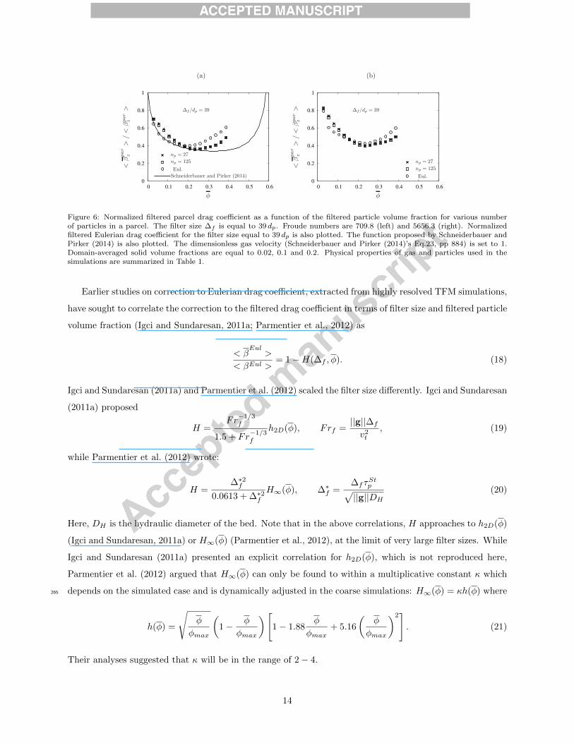
Figure 6a and 6b present the filtered parcel drag correction as a function of filtered particle volume

fraction for two other particle sizes (equivalently, particle Froude numbers). The results are shown for parcel

sizes of 27 and 125, and a filter size of 39dp. The negligible effect of particle coarsening persists for the larger

particles as well. Also shown in these figures are the filtered Eulerian drag corrections. The correlation of245

Schneiderbauer and Pirker (2014) is also plotted in Figure 6a. Once again, the Eulerian and Lagrangian drag

corrections are quite similar in magnitude; in general, the Lagrangian drag coefficient is somewhat larger

(smaller) than the Eulerian one at small (large) filtered particle volume fractions. These could be due to

the fact that the Lagrangian drag coefficient is evaluated at the parcel position, while the Eulerian quantity

is evaluated at the fluid cell center. Irrespective of this distinction, it is clear from Figures 5 and 6 that250

at volume fractions typical of turbulent fluidized beds, coarse MP-PIC and CFD-DPM simulations would

require drag corrections comparable to that required by coarse TFM simulations.

The results presented for the 75µm particles were obtained from simulations with domain-average volume

fraction of 0.02, 0.1 and 0.3. Simulations for the two larger particles with domain-averaged volume fraction

of 0.3 formed nearly one-dimensional, vertically traveling particle plugs, revealing that one would need even255

larger simulation domains to capture three-dimensional structures. At this domain-average volume fractions,

13

Figure 5: Normalized filtered parcel drag coefficient as a function of the filtered particle volume fraction for various number ofparticles in a parcel. The filter sizes ∆f are equal to 21 dp (left) and 39 dp (right). Froude number is 88.4. Normalized filteredEulerian drag coefficient for the filter size equal to 21 dp (left) and 39 dp (right) is also plotted. Physical properties of gas aresummarized in Table 1.

Figure 6a and 6b present the filtered parcel drag correction as a function of filtered particle volume

fraction for two other particle sizes (equivalently, particle Froude numbers). The results are shown for parcel

sizes of 27 and 125, and a filter size of 39dp. The negligible effect of particle coarsening persists for the larger

particles as well. Also shown in these figures are the filtered Eulerian drag corrections. The correlation of

Schneiderbauer and Pirker (2014) is also plotted in Figure 6a. Once again, the Eulerian and Lagrangian drag245

corrections are quite similar in magnitude; in general, the Lagrangian drag coefficient is somewhat larger

(smaller) than the Eulerian one at small (large) filtered particle volume fractions. These could be due to

the fact that the Lagrangian drag coefficient is evaluated at the parcel position, while the Eulerian quantity

is evaluated at the fluid cell center. Irrespective of this distinction, it is clear from Figures 5 and 6 that

at volume fractions typical of turbulent fluidized beds, coarse MP-PIC and CFD-DPM simulations would250

require drag corrections comparable to that required by coarse TFM simulations.

The results presented for the 75µm particles were obtained from simulations with domain-average volume

fraction of 0.02, 0.1 and 0.3. Simulations for the two larger particles with domain-averaged volume fraction

of 0.3 formed nearly one-dimensional, vertically traveling particle plugs, revealing that one would need even

larger simulation domains to capture three-dimensional structures. At this domain-average volume fractions,255

our simulations already involved > 30 million particles and required more than 150 hours of computations on

256 cores; at the present time, anything larger is beyond available resources. Simulations with < φ >= 0.2

for these two particle sizes were found to yield three-dimensional structures (in this simulation domain); as a

result, the results shown for the two larger particle sizes represent averages extracted from simulations with

domain-average volume fraction of 0.02, 0.1 and 0.2.260

13

our simulations already involved > 30 million particles and required more than 150 hours of computations on

256 cores; at the present time, anything larger is beyond available resources. Simulations with < φ >= 0.2

for these two particle sizes were found to yield three-dimensional structures (in this simulation domain); as a

result, the results shown for the two larger particle sizes represent averages extracted from simulations with260

domain-average volume fraction of 0.02, 0.1 and 0.2.

(a) (b)

0

0.2

0.4

0.6

0.8

1

0 0.1 0.2 0.3 0.4 0.5 0.6

φ

<βpar

z>

/<

βpar

z> ∆f/dp = 39

np = 27

np = 125

Eul.

Schneiderbauer and Pirker (2014) 0

0.2

0.4

0.6

0.8

1

0 0.1 0.2 0.3 0.4 0.5 0.6

φ

<βpar

z>

/<

βpar

z> ∆f/dp = 39

np = 27

np = 125

Eul.

Figure 6: Normalized filtered parcel drag coefficient as a function of the filtered particle volume fraction for various number ofparticles in a parcel. The filter size ∆f is equal to 39 dp. Froude numbers are 709.8 (left) and 5656.3 (right). Normalized filteredEulerian drag coefficient for the filter size equal to 39 dp is also plotted. The function proposed by Schneiderbauer and Pirker(2014) is also plotted. The dimensionless gas velocity (Schneiderbauer and Pirker (2014)’s Eq.23, pp 884) is set to 1. Domain-averaged solid volume fractions are equal to 0.02, 0.1 and 0.2. Physical properties of gas and particles used in the simulationsare summarized in Table 1.

Earlier studies on correction to Eulerian drag coefficient, extracted from highly resolved TFM simulations,

have sought to correlate the correction to the filtered drag coefficient in terms of filter size and filtered particle

volume fraction (Igci and Sundaresan, 2011a; Parmentier et al., 2012) as

< βEul

>

< βEul >= 1−H(∆f , φ). (18)

Igci and Sundaresan (2011a) and Parmentier et al. (2012) scaled the filter size differently. Igci and Sundaresan

(2011a) proposed

H =Fr

−1/3f

1.5 + Fr−1/3f

h2D(φ), F rf =||g||∆f

v2t, (19)

while Parmentier et al. (2012) wrote:

H =∆∗2

f

0.0613 + ∆∗2f

H∞(φ), ∆∗f =

∆fτStp√

||g||DH

(20)

Here, DH is the hydraulic diameter of the bed. Note that in the above correlations, H approaches to h2D(φ)

(Igci and Sundaresan, 2011a) or H∞(φ) (Parmentier et al., 2012), at the limit of very large filter sizes.

14

Figure 6: Normalized filtered parcel drag coefficient as a function of the filtered particle volume fraction for various numberof particles in a parcel. The filter size ∆f is equal to 39 dp. Froude numbers are 709.8 (left) and 5656.3 (right). Normalizedfiltered Eulerian drag coefficient for the filter size equal to 39 dp is also plotted. The function proposed by Schneiderbauer andPirker (2014) is also plotted. The dimensionless gas velocity (Schneiderbauer and Pirker (2014)’s Eq.23, pp 884) is set to 1.Domain-averaged solid volume fractions are equal to 0.02, 0.1 and 0.2. Physical properties of gas and particles used in thesimulations are summarized in Table 1.

Earlier studies on correction to Eulerian drag coefficient, extracted from highly resolved TFM simulations,

have sought to correlate the correction to the filtered drag coefficient in terms of filter size and filtered particle

volume fraction (Igci and Sundaresan, 2011a; Parmentier et al., 2012) as

< βEul

>

< βEul >= 1−H(∆f , φ). (18)

Igci and Sundaresan (2011a) and Parmentier et al. (2012) scaled the filter size differently. Igci and Sundaresan

(2011a) proposed

H =Fr−1/3f

1.5 + Fr−1/3f

h2D(φ), F rf =||g||∆f

v2t

, (19)

while Parmentier et al. (2012) wrote:

H =∆∗2f

0.0613 + ∆∗2fH∞(φ), ∆∗f =

∆fτStp√

||g||DH

(20)

Here, DH is the hydraulic diameter of the bed. Note that in the above correlations, H approaches to h2D(φ)

(Igci and Sundaresan, 2011a) or H∞(φ) (Parmentier et al., 2012), at the limit of very large filter sizes. While

Igci and Sundaresan (2011a) presented an explicit correlation for h2D(φ), which is not reproduced here,

Parmentier et al. (2012) argued that H∞(φ) can only be found to within a multiplicative constant κ which

depends on the simulated case and is dynamically adjusted in the coarse simulations: H∞(φ) = κh(φ) where265

h(φ) =

√φ

φmax

(1− φ

φmax

)[1− 1.88

φ

φmax+ 5.16

(φ

φmax

)2]. (21)

Their analyses suggested that κ will be in the range of 2− 4.

14

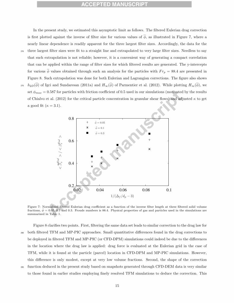
In the present study, we estimated this asymptotic limit as follows. The filtered Eulerian drag correction

is first plotted against the inverse of filter size for various values of φ, as illustrated in Figure 7, where a

nearly linear dependence is readily apparent for the three largest filter sizes. Accordingly, the data for the

three largest filter sizes were fit to a straight line and extrapolated to very large filter sizes. Needless to say270

that such extrapolation is not reliable; however, it is a convenient way of generating a compact correlation

that can be applied within the range of filter sizes for which filtered results are generated. The y-intercepts

for various φ values obtained through such an analysis for the particles with Frp = 88.4 are presented in

Figure 8. Such extrapolation was done for both Eulerian and Lagrangian corrections. The figure also shows

h2D(φ) of Igci and Sundaresan (2011a) and H∞(φ) of Parmentier et al. (2012). While plotting H∞(φ), we275

set φmax = 0.587 for particles with friction coefficient of 0.5 used in our simulations (motivated by the results

of Chialvo et al. (2012) for the critical particle concentration in granular shear flows) and adjusted κ to get

a good fit (κ = 3.1).

While Igci and Sundaresan (2011a) presented an explicit correlation for h2D(φ), which is not reproduced

here, Parmentier et al. (2012) argued that H∞(φ) can only be found to within a multiplicative constant κ265

which depends on the simulated case and is dynamically adjusted in the coarse simulations: H∞(φ) = κh(φ)

where

h(φ) =

√φ

φmax

(1− φ

φmax

)[1− 1.88

φ

φmax+ 5.16

(φ

φmax

)2]. (21)

Their analyses suggested that κ will be in the range of 2− 4.

In the present study, we estimated this asymptotic limit as follows. The filtered Eulerian drag correction

is first plotted against the inverse of filter size for various values of φ, as illustrated in Figure 7, where a270

nearly linear dependence is readily apparent for the three largest filter sizes. Accordingly, the data for the

three largest filter sizes were fit to a straight line and extrapolated to very large filter sizes. Needless to say

that such extrapolation is not reliable; however, it is a convenient way of generating a compact correlation

that can be applied within the range of filter sizes for which filtered results are generated. The y-intercepts

for various φ values obtained through such an analysis for the particles with Frp = 88.4 are presented in275

Figure 8. Such extrapolation was done for both Eulerian and Lagrangian corrections. The figure also shows

h2D(φ) of Igci and Sundaresan (2011a) and H∞(φ) of Parmentier et al. (2012). While plotting H∞(φ), we

set φmax = 0.587 for particles with friction coefficient of 0.5 used in our simulations (motivated by the results

of Chialvo et al. (2012) for the critical particle concentration in granular shear flows) and adjusted κ to get

a good fit (κ = 3.1).280

0.2

0.4

0.6

0.8

0.02 0.04 0.06 0.08 0.1

1/(∆f/dp − 3)

<βEul

z>

/<

βEul

z>

φ = 0.05

φ = 0.1

φ = 0.3

Figure 7: Normalized filtered Eulerian drag coefficient as a function of the inverse filter length at three filtered solid volumefractions, φ = 0.05, 0.1 and 0.3. Froude numbers is 88.4. Physical properties of gas and particles used in the simulations aresummarized in Table 1.

15

Figure 7: Normalized filtered Eulerian drag coefficient as a function of the inverse filter length at three filtered solid volumefractions, φ = 0.05, 0.1 and 0.3. Froude numbers is 88.4. Physical properties of gas and particles used in the simulations aresummarized in Table 1.

Figure 8 clarifies two points. First, filtering the same data set leads to similar correction to the drag law for

both filtered TFM and MP-PIC approaches. Small quantitative differences found in the drag corrections to280

be deployed in filtered TFM and MP-PIC (or CFD-DPM) simulations could indeed be due to the differences

in the location where the drag law is applied: drag force is evaluated at the Eulerian grid in the case of

TFM, while it is found at the particle (parcel) location in CFD-DPM and MP-PIC simulations. However,

this difference is only modest, except at very low volume fractions. Second, the shape of the correction

function deduced in the present study based on snapshots generated through CFD-DEM data is very similar285

to those found in earlier studies employing finely resolved TFM simulations to deduce the correction. This

15

reassures as it indicates robustness of the corrections.

The asymptotic limit deduced by Igci and Sundaresan (2011a) does not allow for dynamic adjustment,

while that due to Parmentier et al. (2012) does. The superior fit seen with the latter model is due to this

adjustable parameter. Parmentier et al. (2012) have also presented an elegant approach to deduce the value290

of this adjustable parameter in coarse simulations. Figure 8 suggests that it would be good to include such

dynamic adjustment of drag coefficient in simulations of filtered TFM, CFD-DPM and MP-PIC simulations.

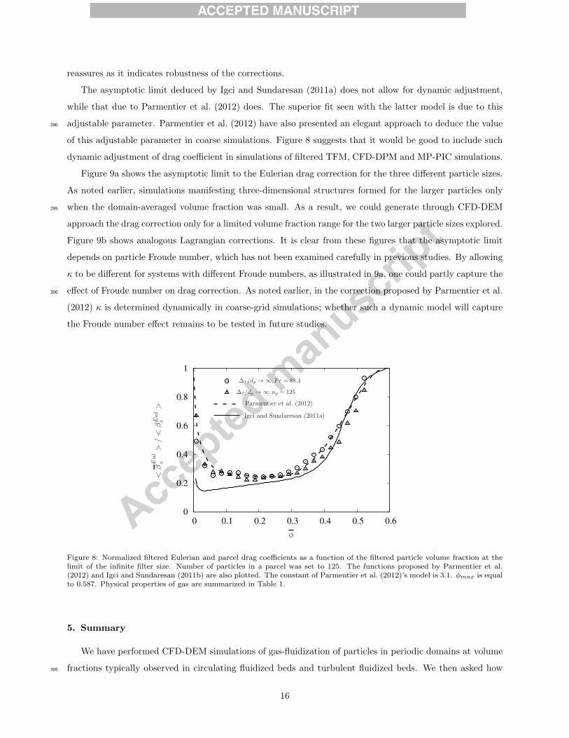
Figure 9a shows the asymptotic limit to the Eulerian drag correction for the three different particle sizes.

As noted earlier, simulations manifesting three-dimensional structures formed for the larger particles only

when the domain-averaged volume fraction was small. As a result, we could generate through CFD-DEM295

approach the drag correction only for a limited volume fraction range for the two larger particle sizes explored.

Figure 9b shows analogous Lagrangian corrections. It is clear from these figures that the asymptotic limit

depends on particle Froude number, which has not been examined carefully in previous studies. By allowing

κ to be different for systems with different Froude numbers, as illustrated in 9a, one could partly capture the

effect of Froude number on drag correction. As noted earlier, in the correction proposed by Parmentier et al.300

(2012) κ is determined dynamically in coarse-grid simulations; whether such a dynamic model will capture

the Froude number effect remains to be tested in future studies.

0

0.2

0.4

0.6

0.8

1

0 0.1 0.2 0.3 0.4 0.5 0.6

φ

<βEul

z>

/<

βEul

z>

∆f/dp → ∞, F r = 88.4

∆f/dp → ∞, np = 125

Parmentier et al. (2012)

Igci and Sundaresan (2011a)

Figure 8: Normalized filtered Eulerian and parcel drag coefficients as a function of the filtered particle volume fraction at thelimit of the infinite filter size. Number of particles in a parcel was set to 125. The functions proposed by Parmentier et al.(2012) and Igci and Sundaresan (2011b) are also plotted. The constant of Parmentier et al. (2012)’s model is 3.1. φmax isequal to 0.587. Physical properties of gas are summarized in Table 1.

(a) (b)

0

0.2

0.4

0.6

0.8

1

0 0.1 0.2 0.3 0.4 0.5 0.6

φ

<βEul

z>

/<

βEul

z>

∆f/dp → ∞, F r = 88.4

∆f/dp → ∞, F r = 709.8

∆f/dp → ∞, F r = 5656.3

H∞(φ)withκ = 3.1

H∞(φ)withκ = 2.8

H∞(φ)withκ = 2.5

0

0.2

0.4

0.6

0.8

1

0 0.1 0.2 0.3 0.4 0.5 0.6

φ

<βLag

z>

/<

βLag

z>

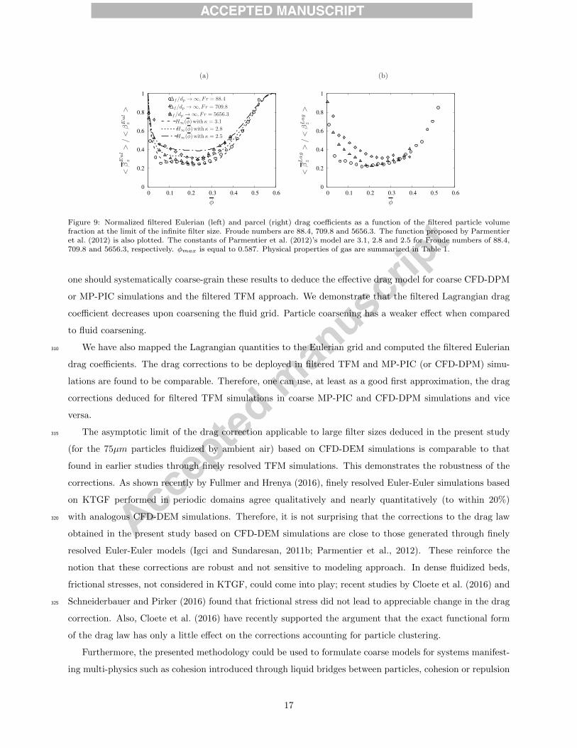
Figure 9: Normalized filtered Eulerian (left) and parcel (right) drag coefficients as a function of the filtered particle volume frac-tion at the limit of the infinite filter size. Froude numbers are 88.4, 709.8 and 5656.3. The function proposed by Parmentier et al.(2012) is also plotted. The constants of Parmentier et al. (2012)’s model are 3.1, 2.8 and 2.5 for Froude numbers of 88.4, 709.8and 5656.3, respectively. φmax is equal to 0.587. Physical properties of gas are summarized in Table 1.

corrections deduced for filtered TFM simulations in coarse MP-PIC and CFD-DPM simulations and vice315

versa.

The asymptotic limit of the drag correction applicable to large filter sizes deduced in the present study

(for the 75µm particles fluidized by ambient air) based on CFD-DEM simulations is comparable to that

found in earlier studies through finely resolved TFM simulations. This demonstrates the robustness of

the corrections. As shown recently by Fullmer and Hrenya (2016), finely resolved Euler-Euler simulations320

17

Figure 8: Normalized filtered Eulerian and parcel drag coefficients as a function of the filtered particle volume fraction at thelimit of the infinite filter size. Number of particles in a parcel was set to 125. The functions proposed by Parmentier et al.(2012) and Igci and Sundaresan (2011b) are also plotted. The constant of Parmentier et al. (2012)’s model is 3.1. φmax is equalto 0.587. Physical properties of gas are summarized in Table 1.

5. Summary

We have performed CFD-DEM simulations of gas-fluidization of particles in periodic domains at volume

fractions typically observed in circulating fluidized beds and turbulent fluidized beds. We then asked how305

16

0

0.2

0.4

0.6

0.8

1

0 0.1 0.2 0.3 0.4 0.5 0.6

φ

<βEul

z>

/<

βEul

z>

∆f/dp → ∞, F r = 88.4

∆f/dp → ∞, np = 125

Parmentier et al. (2012)

Igci and Sundaresan (2011a)

Figure 8: Normalized filtered Eulerian and parcel drag coefficients as a function of the filtered particle volume fraction at thelimit of the infinite filter size. Number of particles in a parcel was set to 125. The functions proposed by Parmentier et al.(2012) and Igci and Sundaresan (2011b) are also plotted. The constant of Parmentier et al. (2012)’s model is 3.1. φmax isequal to 0.587. Physical properties of gas are summarized in Table 1.

(a) (b)

0

0.2

0.4

0.6

0.8

1

0 0.1 0.2 0.3 0.4 0.5 0.6

φ

<βEul

z>

/<

βEul

z>

∆f/dp → ∞, F r = 88.4

∆f/dp → ∞, F r = 709.8

∆f/dp → ∞, F r = 5656.3

H∞(φ)withκ = 3.1

H∞(φ)withκ = 2.8

H∞(φ)withκ = 2.5

0

0.2

0.4

0.6

0.8

1

0 0.1 0.2 0.3 0.4 0.5 0.6

φ

<βLag

z>

/<

βLag

z>

Figure 9: Normalized filtered Eulerian (left) and parcel (right) drag coefficients as a function of the filtered particle volume frac-tion at the limit of the infinite filter size. Froude numbers are 88.4, 709.8 and 5656.3. The function proposed by Parmentier et al.(2012) is also plotted. The constants of Parmentier et al. (2012)’s model are 3.1, 2.8 and 2.5 for Froude numbers of 88.4, 709.8and 5656.3, respectively. φmax is equal to 0.587. Physical properties of gas are summarized in Table 1.

corrections deduced for filtered TFM simulations in coarse MP-PIC and CFD-DPM simulations and vice315

versa.

The asymptotic limit of the drag correction applicable to large filter sizes deduced in the present study

(for the 75µm particles fluidized by ambient air) based on CFD-DEM simulations is comparable to that

found in earlier studies through finely resolved TFM simulations. This demonstrates the robustness of

the corrections. As shown recently by Fullmer and Hrenya (2016), finely resolved Euler-Euler simulations320

17

Figure 9: Normalized filtered Eulerian (left) and parcel (right) drag coefficients as a function of the filtered particle volumefraction at the limit of the infinite filter size. Froude numbers are 88.4, 709.8 and 5656.3. The function proposed by Parmentieret al. (2012) is also plotted. The constants of Parmentier et al. (2012)’s model are 3.1, 2.8 and 2.5 for Froude numbers of 88.4,709.8 and 5656.3, respectively. φmax is equal to 0.587. Physical properties of gas are summarized in Table 1.

one should systematically coarse-grain these results to deduce the effective drag model for coarse CFD-DPM

or MP-PIC simulations and the filtered TFM approach. We demonstrate that the filtered Lagrangian drag

coefficient decreases upon coarsening the fluid grid. Particle coarsening has a weaker effect when compared

to fluid coarsening.

We have also mapped the Lagrangian quantities to the Eulerian grid and computed the filtered Eulerian310

drag coefficients. The drag corrections to be deployed in filtered TFM and MP-PIC (or CFD-DPM) simu-

lations are found to be comparable. Therefore, one can use, at least as a good first approximation, the drag

corrections deduced for filtered TFM simulations in coarse MP-PIC and CFD-DPM simulations and vice

versa.

The asymptotic limit of the drag correction applicable to large filter sizes deduced in the present study315

(for the 75µm particles fluidized by ambient air) based on CFD-DEM simulations is comparable to that

found in earlier studies through finely resolved TFM simulations. This demonstrates the robustness of the

corrections. As shown recently by Fullmer and Hrenya (2016), finely resolved Euler-Euler simulations based

on KTGF performed in periodic domains agree qualitatively and nearly quantitatively (to within 20%)

with analogous CFD-DEM simulations. Therefore, it is not surprising that the corrections to the drag law320

obtained in the present study based on CFD-DEM simulations are close to those generated through finely

resolved Euler-Euler models (Igci and Sundaresan, 2011b; Parmentier et al., 2012). These reinforce the

notion that these corrections are robust and not sensitive to modeling approach. In dense fluidized beds,

frictional stresses, not considered in KTGF, could come into play; recent studies by Cloete et al. (2016) and

Schneiderbauer and Pirker (2016) found that frictional stress did not lead to appreciable change in the drag325

correction. Also, Cloete et al. (2016) have recently supported the argument that the exact functional form

of the drag law has only a little effect on the corrections accounting for particle clustering.

Furthermore, the presented methodology could be used to formulate coarse models for systems manifest-

ing multi-physics such as cohesion introduced through liquid bridges between particles, cohesion or repulsion

17

due to electrostatic charges carried by the particles and cohesion through van der Waals interaction. However,330

it still needs to be firmly established if the findings presented in our current contribution can be transferred

directly to cohesive particulate systems.

In the present study, the drag correction for each gas-particle system is expressed as a function of filter

size and filtered particle volume fraction. Some earlier studies (Milioli et al. (2013); Schneiderbauer et al.

(2013); Ozel et al. (2013)) focusing on drag models for filtered TFM found that the drag correction should335

include additional markers such as local filtered slip velocity. We have not explored such complexities in

the present study. It would be interesting to explore whether additional local markers such as filtered slip

velocity or non-local information such gradients of filtered solid volume fraction and velocities, would improve

quantitative predictions of filtered models.

It would be of interest to analyze CFD-DEM results to formulate filtered stress models and demonstrate340

that they are similar to those found by analyzing TFM results. One can then confidently use the CFD-DEM

approach to develop coarse-grained stress models for systems with complex particle-particle interactions for

which constitutive models needed in TFM are not available.

Acknowledgement

This study was supported by ExxonMobil Research & Engineering Company.345

18

Agrawal, K., Loezos, P.N., Syamlal, M., Sundaresan, S., 2001. The role of meso-scale structures in rapid

gas-solid flows. Journal of Fluid Mechanics 445, 151–185.

Balzer, G., Boelle, A., Simonin, O., 1998. Eulerian gas-solid flow modelling of dense fluidized bed, in:

Fluidization VIII – International symposium of Engineering Foundation, pp. 1125–1134.

Benyahia, S., Sundaresan, S., 2012. Do we need sub-grid scale corrections for both continuum and discrete350

gas-particle flow models? Powder Technology 220, 2–6.

Capecelatro, J., Desjardins, O., 2013. An EulerLagrange strategy for simulating particle-laden flows. Journal

of Computational Physics 238, 1–31.

Capecelatro, J., Desjardins, O., Fox, R.O., 2014a. Numerical study of collisional particle dynamics in cluster-

induced turbulence. Journal of Fluid Mechanics 747, R2.355

Capecelatro, J., Desjardins, O., Fox, R.O., 2016a. Strongly coupled fluid-particle flows in vertical channels.

I. Reynolds-averaged two-phase turbulence statistics. Physics of Fluids (1994-present) 28, 033306.

Capecelatro, J., Desjardins, O., Fox, R.O., 2016b. Strongly coupled fluid-particle flows in vertical channels.

II. Turbulence modeling. Physics of Fluids (1994-present) 28, 033307.

Capecelatro, J., Pepiot, P., Desjardins, O., 2014b. Numerical characterization and modeling of particle360

clustering in wall-bounded vertical risers. Chemical Engineering Journal 245, 295–310.

Chialvo, S., Sun, J., Sundaresan, S., 2012. Bridging the rheology of granular flows in three regimes. Physical

Review E 85, 021305.

Cloete, J.H., Cloete, S., Municchi, F., Radl, S., Amini, S., 2016. The sensitivity of filtered Two Fluid Models

to the underlying resolved simulation setup, in: Fluidization XV – International symposium of Engineering365

Foundation.

Cundall, P.A., Strack, O.D.L., 1979. A discrete numerical model for granular assemblies. Gotechnique 29,

47–65.

Derksen, J.J., Sundaresan, S., 2007. Direct numerical simulations of dense suspensions: wave instabilities in

liquid-fluidized beds. Journal of Fluid Mechanics 587, 303–336.370

Di Renzo, A., Di Maio, F.P., 2004. Comparison of contact-force models for the simulation of collisions in

DEM-based granular flow codes. Chemical Engineering Science 59, 525–541.

Ding, J., Gidaspow, D., 1990. A bubbling fluidization model using kinetic theory of granular flow. AIChE

Journal 36, 523–538.

Fede, P., Simonin, O., 2006. Numerical study of the subgrid fluid turbulence effects on the statistics of heavy375

colliding particles. Physics of Fluids (1994-present) 18, 045103.

19

Fox, R.O., 2014. On multiphase turbulence models for collisional fluidparticle flows. Journal of Fluid

Mechanics 742, 368–424.

Fries, L., Antonyuk, S., Heinrich, S., Dopfer, D., Palzer, S., 2013. Collision dynamics in fluidised bed

granulators: A DEM-CFD study. Chemical Engineering Science 86, 108–123.380

Fullmer, W.D., Hrenya, C.M., 2016. Quantitative assessment of fine-grid kinetic-theory-based predictions of

mean-slip in unbounded fluidization. AIChE Journal 62, 11–17.

Gidaspow, D., 1994. Multiphase Flow and Fluidization: Continuum and Kinetic Theory Descriptions. 1

edition ed., Academic Press, Boston.

Girardi, M., Radl, S., Sundaresan, S., 2016. Simulating wet gassolid fluidized beds using coarse-grid CFD-385

DEM. Chemical Engineering Science 144, 224–238.

Goniva, C., Kloss, C., Deen, N.G., Kuipers, J.A.M., Pirker, S., 2012. Influence of rolling friction on single

spout fluidized bed simulation. Particuology 10, 582–591.

Gu, Y., Ozel, A., Sundaresan, S., 2016. Numerical studies of the effects of fines on fluidization. AIChE

Journal 62, 2271–2281.390

Igci, Y., Andrews, A.T., Sundaresan, S., Pannala, S., O’Brien, T., 2008. Filtered two-fluid models for

fluidized gas-particle suspensions. AIChE Journal 54, 1431–1448.

Igci, Y., Sundaresan, S., 2011a. Constitutive Models for Filtered Two-Fluid Models of Fluidized GasParticle

Flows. Industrial & Engineering Chemistry Research 50, 13190–13201.

Igci, Y., Sundaresan, S., 2011b. Verification of filtered two-fluid models for gas-particle flows in risers. AIChE395

Journal 57, 2691–2707.

Jackson, R., 2000. The Dynamics of Fluidized Particles. Cambridge University Press.

Johnson, K.L., Johnson, K.L., 1987. Contact Mechanics. Cambridge University Press.

Kaufmann, A., Moreau, M., Simonin, O., Helie, J., 2008. Comparison between Lagrangian and mesoscopic

Eulerian modelling approaches for inertial particles suspended in decaying isotropic turbulence. Journal400

of Computational Physics 227, 6448–6472.

Kloss, C., Goniva, C., Hager, A., Amberger, S., Pirker, S., 2012. Models, algorithms and validation for

opensource DEM and CFDDEM. Progress in Computational Fluid Dynamics, an International Journal

12, 140–152.

Kloss, C., Goniva, C., The Minerals, M..M.S.T., 2011. LIGGGHTS Open Source Discrete Element Simula-405

tions of Granular Materials Based on Lammps, in: Supplemental Proceedings. John Wiley & Sons, Inc.,

pp. 781–788.

20

Kobayashi, T., Tanaka, T., Shimada, N., Kawaguchi, T., 2013. DEMCFD analysis of fluidization behavior

of Geldart Group A particles using a dynamic adhesion force model. Powder Technology 248, 143–152.

Koch, D.L., Ladd, A.J.C., 1997. Moderate Reynolds number flows through periodic and random arrays of410

aligned cylinders. Journal of Fluid Mechanics 349, 31–66.

Koch, D.L., Sangani, A.S., 1999. Particle pressure and marginal stability limits for a homogeneous monodis-

perse gas-fluidized bed: kinetic theory and numerical simulations. Journal of Fluid Mechanics 400, 229–263.

Kolehmainen, J., Ozel, A., Boyce, C.M., Sundaresan, S., 2016. A hybrid approach to computing electrostatic

forces in fluidized beds of charged particles. AIChE Journal .415

Li, J., Kwauk, M., 1994. The Energy-Minimization Multi-Scale Method, Metallurgical Industry Press.

Beijing, PR China .

Lun, C.K.K., Savage, S.B., Jeffrey, D.J., Chepurniy, N., 1984. Kinetic Theories for Granular Flow: Inelastic

Particles in Couette Flow and Slightly Inelastic Particles in a General Flowfield. Journal of Fluid Mechanics

140, 223–256.420

Milioli, C.C., Milioli, F.E., Holloway, W., Agrawal, K., Sundaresan, S., 2013. Filtered two-fluid models of

fluidized gas-particle flows: New constitutive relations. AIChE Journal 59, 3265–3275.

Moreau, M., Simonin, O., Bdat, B., 2009. Development of Gas-Particle Euler-Euler LES Approach: A

Priori Analysis of Particle Sub-Grid Models in Homogeneous Isotropic Turbulence. Flow, Turbulence and

Combustion 84, 295–324.425

O’Brien, T.J., 2014. A multiphase turbulence theory for gassolid flows: I. Continuity and momentum

equations with Favre-averaging. Powder Technology 265, 83–87.

OpenFOAM, 2013. OpenFOAM 2.2.2, User Manual .

O’Rourke, P.J., Snider, D.M., 2012. Inclusion of collisional return-to-isotropy in the MP-PIC method.

Chemical Engineering Science 80, 39–54.430

O’Rourke, P.J., Zhao, P.P., Snider, D., 2009. A model for collisional exchange in gas/liquid/solid fluidized

beds. Chemical Engineering Science 64, 1784–1797.

Ozarkar, S.S., Yan, X., Wang, S., Milioli, C.C., Milioli, F.E., Sundaresan, S., 2015. Validation of filtered

two-fluid models for gas-particle flows against experimental data from bubbling fluidized bed. Powder

Technology 284, 159–169.435

Ozel, A., Fede, P., Simonin, O., 2013. Development of filtered EulerEuler two-phase model for circulating

fluidised bed: High resolution simulation, formulation and a priori analyses. International Journal of

Multiphase Flow 55, 43–63.

21

Ozel, A., Vincent, S., Masbernat, O., Estivalezes, J., Abbas, M., Brndle de Motta, J., Simonin, O., 2016. Par-

ticle resolved direct numerical simulation of a Liquid-Solid Fluidized Bed: Comparison with Experimental440

Data. submitted for publication .

Parmentier, J.F., Simonin, O., Delsart, O., 2012. A functional subgrid drift velocity model for filtered drag

prediction in dense fluidized bed. AIChE Journal 58, 1084–1098.

Patankar, N.A., Joseph, D.D., 2001. Modeling and numerical simulation of particulate flows by the Euleri-

anLagrangian approach. International Journal of Multiphase Flow 27, 1659–1684.445

Pepiot, P., Desjardins, O., 2012. Numerical analysis of the dynamics of two- and three-dimensional fluidized

bed reactors using an EulerLagrange approach. Powder Technology 220, 104–121.

Radl, S., Sundaresan, S., 2014. A drag model for filtered EulerLagrange simulations of clustered gasparticle

suspensions. Chemical Engineering Science 117, 416–425.

Rubinstein, G.J., Derksen, J.J., Sundaresan, S., 2016. Lattice Boltzmann simulations of low-Reynolds-450

number flow past fluidized spheres: effect of Stokes number on drag force. Journal of Fluid Mechanics

788, 576–601.

Salikov, V., Antonyuk, S., Heinrich, S., Sutkar, V.S., Deen, N.G., Kuipers, J.A.M., 2015. Characterization

and CFD-DEM modelling of a prismatic spouted bed. Powder Technology 270, Part B, 622–636.

Schneiderbauer, S., Pirker, S., 2014. Filtered and heterogeneity-based subgrid modifications for gas-solid455

drag and solid stresses in bubbling fluidized beds. AIChE Journal 60, 839–854.

Schneiderbauer, S., Pirker, S., 2016. The impact of different fine grid simulations on the sub-grid modification

for gassolid drag, in: 9th International Conference on Multiphase Flow, International Conference on

Multiphase Flow (ICMF): Firenze, Italy.

Schneiderbauer, S., Puttinger, S., Pirker, S., 2013. Comparative analysis of subgrid drag modifications for460

dense gas-particle flows in bubbling fluidized beds. AIChE Journal 59, 4077–4099.

Simonin, O., 1991. Prediction of the dispersed phase turbulence in particle-laden jets.

Snider, D., Banerjee, S., 2010. Heterogeneous gas chemistry in the CPFD EulerianLagrangian numerical

scheme (ozone decomposition). Powder Technology 199, 100–106.

Snider, D.M., 2001. An Incompressible Three-Dimensional Multiphase Particle-in-Cell Model for Dense465

Particle Flows. Journal of Computational Physics 170, 523–549.

Snider, D.M., 2007. Three fundamental granular flow experiments and CPFD predictions. Powder Technology

176, 36–46.

22

Snider, D.M., Clark, S.M., O’Rourke, P.J., 2011. EulerianLagrangian method for three-dimensional thermal

reacting flow with application to coal gasifiers. Chemical Engineering Science 66, 1285–1295.470

Snider, D.M., ORourke, P.J., Andrews, M.J., 1998. Sediment flow in inclined vessels calculated using a

multiphase particle-in-cell model for dense particle flows. International Journal of Multiphase Flow 24,

1359–1382.

Sundaresan, S., 2000. Modeling the hydrodynamics of multiphase flow reactors: Current status and chal-

lenges. AIChE Journal 46, 1102–1105.475

Syamlal, M., Rogers, W., OBrien, T.J., 1993. MFIX documentation: Theory guide. National Energy Tech-

nology Laboratory, Department of Energy, Technical Note DOE/METC-95/1013 and NTIS/DE95000031

.

Tenneti, S., Garg, R., Hrenya, C.M., Fox, R.O., Subramaniam, S., 2010. Direct numerical simulation of

gassolid suspensions at moderate Reynolds number: Quantifying the coupling between hydrodynamic480

forces and particle velocity fluctuations. Powder Technology 203, 57–69.

Tenneti, S., Garg, R., Subramaniam, S., 2011. Drag law for monodisperse gassolid systems using particle-

resolved direct numerical simulation of flow past fixed assemblies of spheres. International Journal of

Multiphase Flow 37, 1072–1092.

Vance, M.W., Squires, K.D., Simonin, O., 2006. Properties of the particle velocity field in gas-solid turbulent485

channel flow. Physics of Fluids (1994-present) 18, 063302.

Vincent, S., Brndle de Motta, J.C., Sarthou, A., Estivalezes, J.L., Simonin, O., Climent, E., 2014. A

Lagrangian VOF tensorial penalty method for the DNS of resolved particle-laden flows. Journal of Com-

putational Physics 256, 582–614.

Wang, J., Ge, W., Li, J., 2008. Eulerian simulation of heterogeneous gas-solid flows in CFB risers: EMMS-490

based sub-grid scale model with a revised cluster description. Chemical Engineering Science 63, 1553–1571.

Wang, W., Li, J., 2007. Simulation of gassolid two-phase flow by a multi-scale CFD approachof the EMMS

model to the sub-grid level. Chemical Engineering Science 62, 208–231.

Wen, C., Yu, Y., 1966. Mechanics of fluidization. Chem. Eng. Prog. Symp. Ser. 62, 100.

Ye, M., van der Hoef, M.A., Kuipers, J.A.M., 2004. A numerical study of fluidization behavior of Geldart A495

particles using a discrete particle model. Powder Technology 139, 129–139.

23