University of Central Florida University of Central Florida

STARS STARS

Electronic Theses and Dissertations, 2004-2019

2009

Flow Visualization In Microfluidic Expansion And Mixing Flow Visualization In Microfluidic Expansion And Mixing

Ehsan Yakhshi-Tafti University of Central Florida, ehsan.yt@gmail.com

Part of the Mechanical Engineering Commons

Find similar works at: https://stars.library.ucf.edu/etd

University of Central Florida Libraries http://library.ucf.edu

This Masters Thesis (Open Access) is brought to you for free and open access by STARS. It has been accepted for

inclusion in Electronic Theses and Dissertations, 2004-2019 by an authorized administrator of STARS. For more

information, please contact STARS@ucf.edu.

STARS Citation STARS Citation Yakhshi-Tafti, Ehsan, "Flow Visualization In Microfluidic Expansion And Mixing" (2009). Electronic Theses and Dissertations, 2004-2019. 4096. https://stars.library.ucf.edu/etd/4096

FLOW VISUALIZATION IN MICROFLUIDIC EXPANSION AND

MIXING

by

EHSAN YAKHSHI-TAFTI

M.S. Amirkabir University of Technology (Tehran Polytechnique, Iran), 2005

A thesis submitted in partial fulfillment of the requirements

for the degree of Master of Science

in the Department of Mechanical Engineering

in the College of Engineering and Computer Science

at the University of Central Florida

Orlando, Florida

Summer Term

2009

Major Professors: Ranganathan Kumar and Hyoung. J. Cho

ii

© Ehsan Yakhshi-Tafti

iii

ABSTRACT

Micro particle image velocimetry (μPIV) is a non-intrusive tool for visualizing flow in

micron-scale conduits. Using this investigative instrument, two experimental studies were

performed to understand flow behaviors in microfluidic channels - a sudden expansion

step flow and laminar velocity profile variation in diffusion driven mixing. First, flow in

a backward facing step feature (1:5 expansion ratio) in a microchannel was taken as the

subject of μPIV flow visualization. The onset and development of a recirculation flow

was studied as a function of flow rate. This flow pattern was further used to investigate

two major parameters affecting μPIV measurements; the depth-of-focus and recording

time-intervals between images in a μPIV image pair. The onset of recirculation was

initiated at flow rates that correspond to Reynolds numbers, Re>95, which is well beyond

the typical working range of microfluidic devices (Re=0.01-10). The recirculation flow

has a 3D structure due to the dimensions of the microchannel and the effect of no slip

condition on the walls. Ensemble cross-correlation was found not to be sensitive to

variations of depth-of-focus and the output flow fields were similar as long as the overall

optical focus remained within the upper and lower bounds of the microchannel. However,

variations of time intervals between images in a μPIV pair, resulted in quantitatively and

qualitatively different flow patterns for a given constant flow rate and depth-of-focus. In

the second experiment, the effect of the laminar velocity profile and its variation on

mixing phenomena at the reduced scale is studied. It is shown that the diffusive mass flux

between two miscible streams, flowing in a laminar regime in a microchannel, is

enhanced if the velocity at their diffusion interface is increased. Based on this idea, an in-

iv

plane passive micromixing concept is proposed and implemented in a working device

(sigma micromixer). This mixer shows considerable mixing performance by periodically

varying the flow velocity profile, such that the maximum of the profile coincides with the

transversely progressing diffusion fronts repeatedly throughout the mixing channel. μPIV

has been used to visualize the behavior of laminar flow inside the micromixer device and

to confirm the periodic variation of the velocity profile through the mixing channel.

v

To Ghazal and Nili

And Mahnaz and Jafar

vi

TABLE OF CONTENTS

INTRODUCTION .............................................................................................................. 1

List of References ........................................................................................................... 9

CHAPTER ONE: SUDDEN EXPANSION STEP FLOW IN A MICROCHANNEL .... 12

Introduction ................................................................................................................... 12

Problem Statement ........................................................................................................ 16

Experimental Setup ....................................................................................................... 20

Results ........................................................................................................................... 22

Onset of Recirculation .............................................................................................. 24

Effect of Depth of Focus ........................................................................................... 26

Effect of Time Interval between PIV Image-Pairs ................................................... 29

Conclusion .................................................................................................................... 31

List of References ......................................................................................................... 33

CHAPTER TWO: DESIGN, FABRICATION AND CHARACTERIZATION OF AN

IN-PLANE PASSIVE MICROMIXER ............................................................................ 35

Introduction ................................................................................................................... 35

Methods and Materials .................................................................................................. 38

Theory ....................................................................................................................... 38

Numerical Simulation ............................................................................................... 44

Fabrication ................................................................................................................ 48

Results - Characterization ............................................................................................. 51

Conclusion .................................................................................................................... 55

List of References ......................................................................................................... 56

vii

APPENDIX A: SU-8 & PDMS PROCESSING – MICROFLUIDIC CHANNEL

FABRICATION ................................................................................................................ 58

APPENDIX B: IMAGE PROCESSING .......................................................................... 67

viii

LIST OF FIGURES

Figure 1 Pressure driven flow in a Hele-Shaw cell (Santiago et al.(Santiago, Wereley et

al. 1998)); Right) µPIV flow visualization using ensemble-averaging measured in a

nominally 300x300µm channel. The solid line is given by analytical solution (Meinhart,

Wereley et al. 1999) ............................................................................................................ 4

Figure 2 a) Acoustic mixing (Liu, Yang et al. 2002) b) Electrokinetic instability mixing

(Oddy, Santiago et al. 2001) c) Mixing enhancement using time pulsing (Glasgow and

Aubry 2003) ........................................................................................................................ 7

Figure 3 Micro particle image velocimetry setup ............................................................. 13

Figure 4 Schematic of a sudden expansion feature in a microchannel (left), top view of an

actual fabricated channel (right) ....................................................................................... 20

Figure 5 TSI microPIV equipment ................................................................................... 21

Figure 6 Laminar flow at a sudden expansion (1:5) feature; due to significant difference

in the velocity magnitude, sections A, B and C were recorded using appropriate time

interval ( t) values (Re=28).............................................................................................. 23

Figure 7 Recirculation zone developing at the backstep wall (Re=280) .......................... 24

Figure 8 Initiation and development of a recirculation zone ............................................ 25

Figure 9 Evolution of the recirculation zone; the dividing streamline migrates from the

backstep wall onto the sidewall of the channel and further downstream as flow rate

increases ............................................................................................................................ 26

Figure 10 μPIV realizations of a recirculation flow at various depths of focus from top to

bottom of the device; (Z*=z/H, D100μsec, Re=222); variation of depth of focus has

insignificant effect on the output flow profile. ................................................................. 28

ix

Figure 11 μPIV realizations using different values of time interval (Dt) between

recordings of the PIV image pairs; depth of focus (Z*=0.5) and flow rate (Re=222) were

held constant. Resulting flow patterns differ qualitatively and quantitatively. ................ 30

Figure 12 Diffusion of species A into liquid film B; C0A is the solubility limit of A in to

liquid B.............................................................................................................................. 39

Figure 13 Progression of diffusion interfaces in the transverse direction to the flow; two

interfaces are developed and move away from the centerline of the channel as one moves

downstream ....................................................................................................................... 41

Figure 14 Velocity profile, unlike in a T-mixer, varies throughout the channel passively

and periodically due to the sidewall design; sidewall profiles expand and contract

asymmetrically (descending slope is steeper than the ascending slope). The velocity

profile maximum, shifts transversely such that it coincides with the diffusion interfaces

repeatedly. Increased velocity at interfaces, results in enhance flux of species. .............. 43

Figure 15 Velocity profiles at A and B resulting from numerical simulations; top layers of

fluid move faster than the bottom layers at section A whereas the situation is reversed at

section B and the velocity profile maximum shifts across the width of the channel. ....... 45

Figure 16 Contour plots of concentration comparing mixing performance of the standard

T mixer and the Modified Sigma micromixer. Ideally, at the exit all cross section

elements should attain a relative concentration of C*=0.5 showing perfect dispersion of

one species in another. ...................................................................................................... 47

Figure 17 Mixing performance deteriorates for mixers as inlet velocity increases

confirming the diffusion-based nature of mixing in microdevices (U*=Umax_inlet / [μ/ρ.Dh]

~ Remax, μ=0.001Pa.sec, ρ=1000kg.m-3

and Dh=100μm) ................................................. 47

x

Figure 18 Actual μPIV flow visualization inside the micromixer; top layers at section A

move slower than the bottom layers of the fluid where as the situation is reversed in

section B. (note the shifting of the velocity profile maximum across the width from A to

B)....................................................................................................................................... 48

Figure 19 General procedure for making microchannel using the SU8 resist and PDMS

replication ......................................................................................................................... 50

Figure 20 Scanning Electron Microscopy (SEM) images of a) oblique view of the

micromixer channel, b) rectangular cross-section of the channel c) smooth surface of the

micromixng walls d) intersection of channel with the reservoir ....................................... 51

Figure 21 Evaluation of mixing performance using color changes as a result of mixing of

a pH indicator (phenolphthalein) and a base solution (sodium hydroxide, pH=12.5)

Performance of Modified Sigma and the Standard T mixers at 3mm mixing length; the

wider the gray region, the better the solutions have mixed( Re=0.4, Q=350μl.hr-1

,

Dhydraulic = 66μm) ............................................................................................................... 52

Figure 22 Mixing performance at a given mixing length (L=8 mm) as a function of flow

Reynolds number, b) Mixing performance at a given flow rate (Q=1000 μl/hr, Re=0.91)

as a function of mixing length. ......................................................................................... 54

Figure 23 Two layers of PDMS (top: blank - bottom: with patterns) are bonded to form a

closed microchannel; inlet and outlet ports are punched in the blank layer prior to

bonding ............................................................................................................................. 65

Figure 24 Corona surface treatment machine is used to bond pdms-pdms or pdms-glass

layers ................................................................................................................................. 65

Figure 25 Infusion pump with control keypad .................................................................. 70

xi

Figure 26 Initial image correction / enhancement ............................................................ 71

Figure 27 Grayscale intensity across the channel width (Note: black color Imin=0). For

ideal mixing all pixel should attain a grayscale intensity of 0 showing the gray band has

expanded over the entire channel width............................................................................ 72

Figure 28 Sequence of steps in image processing for mixing evaluation ......................... 73

1

INTRODUCTION

Microfluidics research and technology is an emerging interdisciplinary field developed at

the intersection of chemistry, life sciences and physics (mainly fluid mechanics).

Microfluidics involves study of the behavior of fluids flowing in very small conduits,

typically at micrometer scales. Microfluidic devices and applications often involve

minute volumes of fluid and transport processes which are dominated by molecular

diffusion and not inertial effects. As the length of a system is scaled down, surface (L2) to

volume (L3) ratio in a system increases indicating that surface and interfacial effects gain

more significance compared to body forces such as inertia. For example a ten fold

decrease in the characteristic length will reduce the surface 100 fold, and the volume to

get smaller 1000 times; however the surface to volume ratio would increase 10 fold

compared to the original ratio. The behavior of fluids at the reduced scale is highly

influenced by factors such as surface tension, energy dissipation, quick thermal relaxation

and fluidic resistance. By scaling down a system many new applications have been

explored, in spite of challenges and shortcomings in actual realization of such systems.

For example, fluids flowing side-by-side, do not necessarily mix in the traditional sense;

molecular transport between them must often be through diffusion, a relatively slow

process.

Fundamental science regarding fluid flow at reduced scales as well as applied technology

targeted toward use in biochemical analytical systems are topics of ongoing research.

Study of slip conditions on surfaces for gas and liquid flows (Lockerby, Reese et al.

2

2004; Lauga, Brenner et al. 2007), effects of miniaturizing on emulsions and surfactant

functionality (Thorsen, Roberts et al. 2001), breakup of nano-jets (Moseler and Landman

2000), multiphase (liquid/liquid and liquid/gas) micro-flows (Stone, Stroock et al. 2004),

anomalous diffusion (Basu, Wolgemuth et al. 2004), hydrodynamic dispersion and

diffusion in non-newtonian systems (Daniel 2001) boiling regimes in microchannels

(Kandlikar 2002), microsystems with chaotic flow (Yi-Kuen, Deval et al. 2001) and

adsorption (physical/chemical) phenomena (Huber, Manginell et al. 2003) are some of

the active areas of fundamental research using microfluidic devices and concepts.

Development of inkjet printers, DNA sequencing chips, lab-on-a-chip technology and

thermal microdevices are some examples of applied microfluidics.

Flow visualization has been essential to the development of the field of microfluidics. As

the name microfluidics implies, the channels and conduits that contain the flows are

extremely small and insertion of any kind of probes into the devices for flow

measurement is usually impractical. Non-invasive flow visualization is important for the

fundamental understanding of the nature of micro-flows, analysis and development of

novel microfluidic devices, study of the related phenomena and providing data for

validation of computer aided simulation results (Sinton 2004). Particle-based

visualization techniques have been widely practiced in the field of microfluidics and

involve dispersion of tracking particles in the fluids. These particles can follow the fluid

reasonable well and velocity of fluids is inferred from recording the motion of the

particles. Laser Doppler Anemometry (LDA) Particle Image Velocimetry (PIV) and

Particle Streak Velocimetry (PSV) are major particle-based techniques that are used for

3

non-invasive flow visualization. In LDA, illumination from two laser sources form an

optical interference intersection; passage of highly reflective tracking particles through

the illumination volume causes shifts in the interference fringes. Displacement of the

fringes divided by time gives the velocity of fluid at the illumination spot. This method is

mostly used for macro scale applications as a number of complications arise when length

scales are reduced (Tieu, Mackenzie et al. 1995). In PSV, streaks of particles (e.g.

fluorescent dye) are tracked over a period of time on a single image. This technique has

very low resolution and only provides sparse information for the velocity field but

requires less experimental infrastructure (Brody, Yager et al. 1996). In PIV, the flow

domain is illuminated by generating a two dimensional light sheet (macro scale) or

illumination of a volume of fluid by a single frequency light such as Nd:YAG laser. Two

consecutive images are taken at a known time interval and resulting images are compared

using cross-correlation (two frames) or auto-correlation (single frame) algorithms. Micro

PIV (µPIV) is a derivative of PIV technique adapted for micro flow visualization. First

studies in the area of µPIV were conducted by Santiago et al. followed by Meinhart et al.

(Figure 1) and Koutsiaris (Koutsiaris, Mathioulakis et al. 1999) and other researchers.

4

Figure 1 Pressure driven flow in a Hele-Shaw cell (Santiago et al.(Santiago, Wereley et al. 1998));

Right) µPIV flow visualization using ensemble-averaging measured in a nominally 300x300µm

channel. The solid line is given by analytical solution (Meinhart, Wereley et al. 1999)

There are three key alterations from PIV to µPIV(Meinhart, Wereley et al. 1999):

First: since the flow passages are micron size; in this case, Brownanian motion can be a

noise generating factor because the random motion of particles are in the order of the

limited displacements of the particles due to the bulk motion of the fluid.

Second: dimension of flow passage are in micrometer range; hence the particles used for

visualization are even smaller. Complications arise in imaging such particles that have

diameters on the order of the illumination light wavelength (for example Nd:YAG laser

produces 532 nm wavelength light).

Third: due to size limitations it is not possible to generate two-dimensional light sheets

that only illuminate particles on a 2D plane inside the flow. Rather, a three dimensional

volume is illuminated. In this case, particles above and below the focal plane get

illuminated and eventually contribute to the noise. While out of focus particles are not in

the same plane as the in-focus particles, yet they would contribute to the velocity

5

measurement algorithm. This issue is has been addressed in the present manuscript.The

light coming from particles off the plane of focus forms a background noise (glow) which

makes it difficult to distinguish between light coming from in-focus particles and that

from the off-focus particles. Problems arising due to volume illumination issues in µPIV

have been studied by (Meinhart, Wereley et al. 2000), (Olsen and Adrian 2000), (Ovryn

2000) and (Cummings 2000). Details of these studies are given in the dedicated chapter.

In the first chapter of this study, the effect of depth of focus and varying time intervals

between images of a double-frame pair on the Ensemble cross-correlation µPIV scheme

is found by using the backward facing step (sudden expansion) flow as the subject of

flow imaging. Recirculation and vortex generation are distinct features of sudden

expansion flows. Onset of recirculation and development of vortices has been studied

using µPIV. Further more, this flow pattern has been used a subject to investigate

technical parameters of the imaging system, namely the depth of focus and time intervals

between pair images. As mentioned earlier, flow visualization is of key importance in

studying flow behavior at reduced scales and investigation of issues related to µPIV - a

major technique for flow imaging in micro flows - is useful and necessary.

Moving on to the applications of microfluidics, it is noted that in majority of cases

especially in analytical lab on chips, mixing of two or more fluids is essential to

achieving the application goals. Microfluidic devices are mainly designed for chemical

and biological applications where rapid and efficient mixing is essential. Mixing is of

considerable importance to realizing lab-on-a-chip (LOC) bio-analysis systems since a

6

majority of the applications often involve reactions that require quick and efficient

mixing of reactants for initiation (Liu, Stremler et al. 2000). Nevertheless, mixing is greatly

limited at the microscale where fluid flow is almost in all cases laminar. In laminar flows,

layers of fluid co-flow and slide over their neighboring layers in a parallel manner

without motion in the transverse direction. Considering the Highly laminar nature of flow

and the fact that introduction of chaos and turbulence cannot be easily achieved or may

not be practical under design constraints, it is expected that rapid mixing cannot be

readily achieved in microfluidic devices. This limitation is the motivation for designing

novel micromixing concepts.

Micromixer designs are categorized based on the source of energy used to perform

mixing. Active mixers are stimulated by external sources of energy, while passive mixers

achieve mixing based on geometrical design of the mixing channels (Nguyen and Wu

2005). In the former class, external sources such as acoustic (Liu, Yang et al. 2002),

thermal (Tsai and Lin 2002), electrokinetic (Oddy, Santiago et al. 2001) and pressure

disturbances (Deshmukh, Liepmann et al. 2001) cause stirring effects that enhance

mixing of reagents (Figure 2). While active micromixers have better mixing performance

compared to passive mixers, complications in integrating the external stimulus

mechanisms and the required power sources into the microdevices make them expensive

and incompatible to most applications; especially in cases where cheap disposable

platforms are desired. Majority of passive mixers are designed based on various channel

geometries in which external power sources are not required and the streaming flow itself

creates mixing (Liu, Stremler et al. 2000; Lee, Kim et al. 2006). Due to fabrication and

7

cost issues, 2D (planar) passive micromixers are preferred over those with complex three

dimensional structures (Jessica Melin 2004).

Figure 2 a) Acoustic mixing (Liu, Yang et al. 2002) b) Electrokinetic instability mixing (Oddy,

Santiago et al. 2001) c) Mixing enhancement using time pulsing (Glasgow and Aubry 2003)

In the second chapter, micromixing has been studied theoretically and based on the

findings an in plane passive micromixer has been designed, fabricated and tested for

mixing performance. Numerical simulations were conducted to evaluate the mixing

concept. Laminar velocity profile variation in the mixing channel is a key feature of the

8

mixer; µPIV studies developed in this study have been used to visualize the flow and

verify the periodic variation of flow in the mixing device.

Fabrication of devices was done in the clean room facilities in-house. Details of

fabrication, testing and image processing performed as part of the characterization are

documented and given as appendices.

9

List of References

Basu, S., C. W. Wolgemuth, et al. (2004). "Measurement of Normal and Anomalous

Diffusion of Dyes within Protein Structures Fabricated via Multiphoton Excited Cross-

Linking." Biomacromolecules 5(6): 2347-2357.

Brody, J. P., P. Yager, et al. (1996). "Biotechnology at low Reynolds numbers."

Biophysical Journal 71(6): 3430-3441.

Cummings, E. B. (2000). "An image processing and optimal nonlinear filtering technique

for particle image velocimetry of microflows." Experiments in Fluids 29(7): S042-S050.

Daniel, A. B. (2001). "Taylor dispersion of a solute in a microfluidic channel." Journal of

Applied Physics 89(8): 4667-4669.

Deshmukh, A., D. Liepmann, et al. (2001). Continuous micromixer with pulsatile

micropumps. Solid-State Sensor and Actuator Workshop, Hilton Head Island.

Glasgow, I. and N. Aubry (2003). "Enhancement of microfluidic mixing using time

pulsing." Lab Chip 3: 114-120.

Huber, D. L., R. P. Manginell, et al. (2003). "Programmed Adsorption and Release of

Proteins in a Microfluidic Device." Science 301(5631): 352-354.

Jessica Melin, G. G., Niclas Roxhed, Wouter van der Wijngaart and Göran Stemme

(2004). "A fast passive and planar liquid sample micromixer." Lab on a Chip.

Kandlikar, S. G. (2002). "Fundamental issues related to flow boiling in minichannels and

microchannels." Experimental Thermal and Fluid Science 26(2-4): 389-407.

Koutsiaris, A. G., D. S. Mathioulakis, et al. (1999). "Microscope PIV for velocity-field

measurement of particle suspensions flowing inside glass capillaries." Measurement

Science and Technology(11): 1037.

10

Lauga, E., M. P. Brenner, et al. (2007). Microfluidics: The no-slip boundary condition.

Handbook of Experimental Fluid Dynamics (Chapter 19), Springer.

Lee, S. W., D. S. Kim, et al. (2006). "A split and recombination micromixer fabricated in

a PDMS three-dimensional structure." Journal of Micromechanics and Microengineering

16(5): 1067-1072.

Liu, R. H., M. A. Stremler, et al. (2000). "Passive Mixing in a Three-Dimensional

Serpentine Microchannel." Journal of Microelectromechanical Systems 9: 190-197.

Liu, R. H., J. Yang, et al. (2002). "Bubble-induced acoustic micromixing." Lab on a Chip

2: 151-157.

Lockerby, D. A., J. M. Reese, et al. (2004). "Velocity boundary condition at solid walls

in rarefied gas calculations." Physical Review E 70(1): 017303.

Meinhart, C. D., S. T. Wereley, et al. (2000). "Volume illumination for two-dimensional

particle image velocimetry." Measurement Science and Technology(6): 809.

Meinhart, C. D., S. T. Wereley, et al. (1999). "PIV measurements of a microchannel

flow." Experiments in Fluids 27(5): 414-419.

Moseler, M. and U. Landman (2000). "Formation, Stability, and Breakup of Nanojets."

Science 289(5482): 1165-1169.

Nguyen, N.-T. and Z. Wu (2005). "Micromixers-a review." Journal of Micromechanics

and Micorengineering 15: R1.

Oddy, M. H., J. G. Santiago, et al. (2001). "Electrokinetic Instability Micromixing."

Analytical Chemistry 73(24): 5822-5832.

11

Olsen, M. G. and R. J. Adrian (2000). "Out-of-focus effects on particle image visibility

and correlation in microscopic particle image velocimetry." Experiments in Fluids 29(7):

S166-S174.

Ovryn, B. (2000). "Three-dimensional forward scattering particle image velocimetry

applied to a microscopic field-of-view." Experiments in Fluids 29(7): S175-S184.

Santiago, J. G., S. T. Wereley, et al. (1998). "A particle image velocimetry system for

microfluidics." Experiments in Fluids 25(4): 316-319.

Sinton, D. (2004). "Microscale flow visualization." Microfluidics and Nanofluidics 1(1):

2-21.

Stone, H. A., A. D. Stroock, et al. (2004). "ENGINEERING FLOWS IN SMALL

DEVICES: Microfluidics Toward a Lab-on-a-Chip." Annual Review of Fluid Mechanics

36(1): 381-411.

Thorsen, T., R. W. Roberts, et al. (2001). "Dynamic Pattern Formation in a Vesicle-

Generating Microfluidic Device." Physical Review Letters 86(18): 4163.

Tieu, A. K., M. R. Mackenzie, et al. (1995). "Measurements in microscopic flow with a

solid-state LDA." Experiments in Fluids 19(4): 293-294.

Tsai, J.-H. and L. Lin (2002). "A thermal-bubble-actuated micronozzle-diffuser pump."

Journal of Microelectromechanical Systems 11(6): 665-671.

Yi-Kuen, L., J. Deval, et al. (2001). Chaotic mixing in electrokinetically and pressure

driven micro flows. Micro Electro Mechanical Systems, 2001. MEMS 2001. The 14th

IEEE International Conference on.

12

CHAPTER ONE: SUDDEN EXPANSION STEP FLOW IN A MICROCHANNEL

Introduction

Particle Image Velocimetry (PIV) can be used to obtain high-resolution 2-D velocity

fields (Meinhart, Wereley et al. 1998). In conventional PIV, the flow is seeded with tracer

particles that scatter light due to having a refractive index different from that of the fluid

or because of fluorescence properties. Laser light is usually used as a source of

illumination. By means of the special configuration of optics, the flow is illuminated in a

2D light sheet at the desired location of the flow. The tracer particles, which reasonably

follow the fluid flow, are photographed at consecutive instances with a known time

interval. Each pair of the double-frame image is subdivided into smaller regions called

the interrogation spots. The displacement of the particles within the interrogation spot is

derived based on statistical methods with high accuracy (0.1 pixels) which results in

visualization of the velocity field in the illuminated 2D plane with knowledge of the time

interval (Nguyen and Wereley 2002).

Micro particle image velocimetry (μPIV) is a useful tool in studying fluid mechanics at

the reduced scale (micrometer range) also known as microfluidics. In conventional PIV,

with the proper selection of optics, it is possible to illuminate particles in the flow on a

desired 2D plane. The thickness of the illumination light sheet is much smaller than the

characteristic dimensions of the flow; for example the width/height of a duct. Therefore,

the flow can be analyzed layer by layer. In μPIV however, all the particles in the flow

field are illuminated due to limited optical access; the intensity of light picked up by the

tracer particles varies depending on how far away they are from the plane of focus. Epi-

fluorescence technique is implemented in μPIV, since the limited optical access does not

13

allow illumination and collection of the excitation and re-emission light from two

separate paths. Fluorescent dyes offer the possibility of using only one optical pathway.

Excitation light from an Nd:Yag laser with a fixed wavelength is guided to the desired

location of the flow; fluorescent dyes absorb this light moving into an excitation mode; at

releasing the absorbed energy, they re-emit light at a higher wavelength, since part of the

original energy gets dissipated as heat. The re-emission light can be filtered out using a

dichroic mirror that is transparent to the wavelength used for excitation but reflective to

the re-emission wavelength. The re-emission light is guided to the CCD camera where

the images are recorded in pairs and eventually transmitted to a computer for further

processing (Figure 3).

Figure 3 Micro particle image velocimetry setup

The fact that all particles in the field of view are illuminated and contribute to the final

image can be a major problem. The light from particles off the plane of focus forms a

background noise (glow) which makes it difficult to distinguish between light coming

from in-focus particles and that from the off-focus particles. Micro particle image

14

velocimetry technique is different from the conventional PIV in three ways; 1) tracer

particles are in the size range of the wavelength of the illumination light, which can make

the visualization of microflows challenging; 2) Brownian random motion of tracing

particles can be a significant source of error in low rates of flow 3) illumination of the

flow is not in a 2D plane but is rather an illumination volume; hence, out of focus

emissions from particles below and above the depth of focus increase the noise to signal

ratio. Santiago et al. first used PIV for microfluidic flows by using the concept of epi-

fluorescence (Santiago, Wereley et al. 1998). Due to the extremely small dimensions and

complexities of flow measurement in small scales (micro and nano meter scales), not

many successful experimental studies have been conducted that give details of the flow

such as the velocity and pressure fields and their derivatives. However,

Devasenathipathy, Santiago et al. 2002, Santiago and Meinhart Santiago, Wereley et al.

1998 have characterized such flow patterns in the micron scale devices.

In the present work, fluorescent dyed polystyrene tracer particles with an average

diameter of 1.1 μm were used. The absorption wavelength peak is 540nm and re-emission

is at a longer wavelength of 560nm for these particles. The emission light level is affected

by the fluorophore concentration, particle size, illumination wavelength, pulse energy,

pulse duration and the optical filters. The illumination source used here is a Q-switch Nd-

Yag laser that generates 532nm wavelength light. With the epi-fluorescent technique the

illumination and re-emission light to and from the measurement location, have identical

pathways except after the epi-fluorescence filter cube. The filter cube containing a

dichroic mirror and barrier filter is used to direct the illumination light and the re-

emission light to and from the fluorescent particles so that the fluorescent re-emission

15

gets filtered out and guided to the CCD camera which records the images and transmits

them to a computer for processing. Increasing the fluorescent particle concentration will

increase the concentration of particles in the image, but since a volume of fluid is

illuminated rather than a 2D sheet, light picked up from out of focus particles may

increase the background noise level. The laser light pulse duration is fixed to a value

between 3 to 10 nano-seconds. Increasing laser pulse energy also increases the emission

level but only to a certain threshold level after which no additional emission will be

added. The double frame image pairs are further processed with cross correlating

algorithms and the velocity vector field is derived. Ensemble correlation processing is

used which is appropriate for visualization of steady flow patterns. Double-frame image

pairs obtained in μPIV are processed by cross-correlation schemes which are often

written in the form of a computer code in order to resolve the velocity field from the

motion of the vase number of illuminated particles. The purpose of this study is to

evaluate the sensitivity of the Ensemble Cross-correlation algorithm to the optical focus

depth and variation of time intervals between image pairs. This scheme is mostly used for

processing steady flows. The correlation function at a certain interrogation spot is

generally represented by the following set of equations (Gad-el-Hak 2005):

q

j

p

i

kkk njmigjifnm

1 1

),().,(),(

1

Where f and g are the gray value of the gray value distribution from the first and second

exposure for the kth

recording PIV recording pair for an interrogation spot of size (p x q)

pixels. The highest peak of this function occurs at the particle image displacement in the

interrogation spot. If the flow has a steady characteristic, then the main peak of Φk(m,n)

always occurs at the same position for PIV recording pairs recorded at different times,

16

whereas all other sub-peaks occur with random intensities and positions in different

recording double frame pairs. If a large number of pairs is taken together (ensemble) and

averaged, then the main peak will remain at the same location and the random peaks

(noise) will average out to zero. The average (ensemble) correlation is given as

N

k

kens nmN

nm1

),(1),( 2

Once the displacement is found in an interrogation spot, given the time interval the

velocity vectors can be plotted. Fifty pair images were required on average to yield

quality vector fields. The time interval between frames of a pair depends on the

magnitude of the velocity of the tracer particles. It is noted that if the velocities in the

photographed area vary significantly compared to each other, then different time intervals

should be used to capture various ranges of velocity magnitudes; for example, small time

intervals are required to track fast moving tracer particles and larger time intervals to

capture the slow moving tracers.

Problem Statement

In conventional PIV, with the proper selection of optics, it is possible to illuminate

particles in the flow on a desired 2D plane. The thickness of the illumination light sheet is

much smaller than the characteristic dimensions of the flow; for example the width/height

of a duct. Therefore the flow can be analyzed layer by layer. In μPIV however, all the

particles in the flow field are illuminated due to limited optical access; the intensity of

light picked up by the tracer particles varies depending on how far away they are from the

plane of focus. Epi-fluorescence technique is implemented in μPIV, since the limited

optical access does not allow illumination and collection of the excitation and re-emission

light from two separate paths. Fluorescent dyes offer the possibility of using only one

17

optical pathway. Excitation light from an Nd:Yag laser with a fixed wavelength is guided

to the desired location of the flow; fluorescent dyes absorb this light moving into an

excitation mode; at releasing the absorbed energy, they re-emit light at a higher

wavelength, since part of the original energy gets dissipated as heat. The re-emission

light can be filtered out using a dichroic mirror that is transparent to the wavelength used

for excitation but reflective to the re-emission wavelength. The light from particles off

the plane of focus forms a background noise (glow) which makes it difficult to

distinguish between light coming from in-focus particles and that from the off-focus

particles. Olsen and Adrian (Olsen and Adrian 2000; Olsen and Adrian 2000) introduced

the concept of particle visibility for μPIV measurements while addressing this issue.

Particles were considered to be visible if only their peak intensity in the recorded images

rose significantly above the background glow. Particle visibility was found to be weakly

dependent on magnification, and most readily increased by decreasing the f number of the

optical system; depth-of-field increases with increasing the f-number. This means that

images taken with a low f-number will tend to have limited number of particles in focus,

with the rest being out of focus; hence eliminating the contribution of non-visible (out of

focus particles) to the image. If the optical parameters are kept constant, then particle

visibility can be increased by either decreasing the depth of the microfluidic device or

using a lower particle concentration. However, using lower particle concentration will

have the effect of reducing the number of particles within each interrogation volume

resulting in noisier velocity estimates. In addition, reduced concentration of fluorescent

dye can possibly necessitate using larger interrogation spots resulting in lower spatial

resolution. Meinhart et al. (Carl, Steve et al. 2000; Meinhart, Wereley et al. 2000)

18

maintained high spatial resolution at low particle concentration by taking many

realizations and then averaging the calculated spatial correlations for each interrogation

region to yield a high-vector-density velocity field. This technique is limited to steady

flows or periodic flows with phase locking. It is important to note that usually the

measured velocity is found to be a weighted average over the depth of the fluidic device.

By using appropriate weighting functions, velocity variation from top to bottom of the

interrogation volume can be accounted for. The weighting function can be used to put a

bound on the interrogation volume (depth of correlation) by defining a distance from the

object plane beyond which particles no longer contribute to the correlation function

significantly. As a solution for the background noise reduction, Bourdon et al. (Bourdon,

Olsen et al. 2004) proposed an image filtering method, termed power-filtering for

controlling the depth of correlation, independent of the image acquisition system, particle

size, and flow characteristics. By choosing appropriate power values, it is possible to

increase or decrease the depth of correlation by a factor two.

In this study, the effect of depth of focus and varying time intervals between images of a

double-frame pair on the Ensemble cross correlation scheme is found. Backward facing

step in a rectangular cross section microchannel having a hydraulic diameter of 133

microns, by means of the particle image velocimetry technique and implementing the

Ensemble method.

Recirculation and flow separation is the main feature of flow at sudden expansion

geometries in internal macroscopic flows. This unique flow pattern offers an opportunity

to investigate the characteristics of the above mentioned scheme in resolving velocity

profiles in microchannels. Sudden expansion (backward facing step) flows are among

19

commonly encountered basic flow patterns that have been addressed widely by

researchers by means of theoretical, numerical and experimental methods in laminar and

turbulent flow regimes in the macro-scale. Flow created at backward facing steps is of

importance because it gives insight to many internal flow patterns generated at

geometries containing sudden expansions in the path of flow; phenomena such as flow

separation and recirculation and their effects on heat and mass transfer can be analyzed

with reference to this flow pattern. Armaly et al. (Armaly, Durst et al. 1983) used Laser-

Doppler anemometry to make comprehensive measurements on air flows over a

backward facing step in a test channel over a 70-8000 range of Reynold’s number

covering laminar, transitional, and turbulent flows. Many numerical works have also been

reported on this subject. Biswas et al. (Biswas, Breuer et al. 2004) studied the backward

facing step flow for expansion ratios of 1.95, 2 and 3 and provided information on

characteristic flow patterns for Re of 10-4

to 800.

Here, the effect of variation of the depth-of-focus applied by adjusting the microscope

focus and the time intervals between PIV image-pairs is found on the flow visualization

using µPIV. Results at transition to recirculation flow for backward facing step for a 1:5

expansion is also provided.

20

Figure 4 Schematic of a sudden expansion feature in a microchannel (left), top view of an actual

fabricated channel (right)

Experimental Setup

The microfluidic device used for this study is fabricated using the well established SU-8

photolithography and Polydimethylsiloxane (PDMS) replication techniques (Jo, Van

Lerberghe et al. 2000). The device pattern is transferred via photolithography from a

mask onto the silicon wafer which has been spin-coated with SU-8 photoresist. The

developed SU-8 on the wafer is used as a mold; PDMS with a curing agent is poured on

the mold and allowed to cure overnight at room temperature. The PDMS layer with cast

features is then bonded to another flat piece of PDMS or glass slide by plasma surface

treatment. The device consists of a straight channel with a rectangular cross section that

suddenly expands to a larger width (1:5 ratio). Recirculation flow occurs as the flow

suddenly expands. The width to height ratio is 10:1 (x: flow direction, z: depth)

downstream the expansion (Figure 4). Since the bottom and top walls influence the flow

due to the no slip boundary condition, then choosing the appropriate depth of focus

would be a determining factor on the flow profile; this gives significance to the depth-of-

focus. For example, closer to the walls, the vortex would have smaller radius with lower

velocity magnitudes compared to the center portion that is less influenced by the walls.

z

y

x

100 μm

200μm

z

y

21

The μPIV (TSI Inc. MN) apparatus consisted of the following major components;

Nd:Yag laser source that generates green light at a wavelength of 532nm. Nikon

(TE2000-S) inverted microscope is used for magnifying the flow field which is

compatible with the epi-fluorescent technique (Figure 5).

Figure 5 TSI microPIV equipment

A 10x magnifying objective lens was used. A barrier filter cube was used to filter out the

re-emission light from the excitation light. Polystyrene fluorescent dye was used in this

study as the tracer particle with the following properties: 1μm average diameter, 540nm

excitation /560nm re-emission wavelength, 1010

beads/mL (FluroSpheres, Invitrogen CA).

A CCD camera was used to capture PIV images, capable of acquiring image-pairs at

maximum 15 double-image frames per second, with time intervals between two images

of a frame as low as 1μs. The timings of the laser firing and image capture are controlled

by a synchronizer unit. Ensemble cross correlation scheme together with background

conditioning was used for deriving the flow field from the captured images. An average

Laser Power Supply

Synchronizer Laser Head Inverted Microscope

Syringe Pump

Camera

22

of N=50 double-frame image pairs were processed for each case of variable time interval,

depth of focus or change in flow rate. Flow through the microchannels is maintained and

controlled by a precision syringe pump (KD Scientific, MA). Flow rate is varied such that

the onset and development of recirculation is observed at the backstep feature. The effect

of each variable is systematically investigated by maintaining all other variables and

parameters constant.

Results

A typical characteristic of sudden expansion flows is the vortices and recirculation flow

generated downstream the expansion feature. In microfluidic devices however, the

circulation zone is absent in the typical range of micro-flows (Re=ρUDH/μ= 0.01-10).ρ

and μ are density and viscosity of the fluid where U and DH are average flow velocity and

hydraulic diameter, respectively., laminar flow without any disturbances (Re=28) and a

fully developed recirculation (Re=280) are shown in (Figure 6, Figure 7), respectively.

All experiments were carried out using identical tracer particle concentrations. Each

variable was varied holding the others constant. The hydraulic diameter is calculated for

the rectangular cross section at the entrance channel, upstream of the expansion feature.

PADH 4

3

Where A and P are the area and perimeter of the cross section, respectively. Note that for

visualizing of each portion of the flow, depending on the magnitude of velocity,

appropriate time intervals should be used. For example, in figure 6, the fast moving core

is recorded using 75μs time interval, whereas for the slow moving flow at the corners

away from the center, time intervals of 200 and 600 micro seconds, were used in section

B and C respectively.

23

Figure 6 Laminar flow at a sudden expansion (1:5) feature; due to significant difference in the

velocity magnitude, sections A, B and C were recorded using appropriate time interval ( t) values

(Re=28)

The first signs of recirculation appear at a flow rate of 950μL.min-1

. Using physical

properties of water and the hydraulic diameter as the characteristic length, the

corresponding Reynolds number, Re=95 at the onset of recirculation at the given plane of

flow. It should be noted that the critical Re can vary from one plane to another with a

different depth (z) since the flow has 3D structure. This range of Re numbers is fairly

large, compared to typical microfluidic flows.

C B

A A

Δt=75μs

C

Δt=600μs

B

Δt=200μs

24

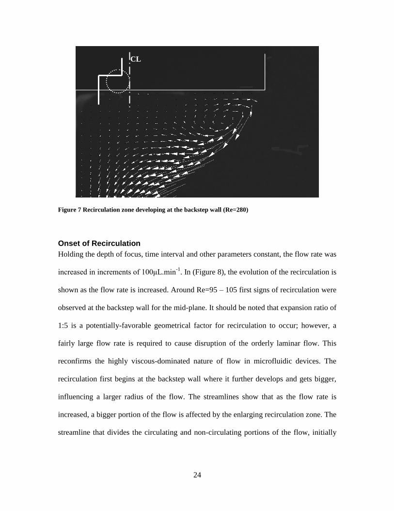
Figure 7 Recirculation zone developing at the backstep wall (Re=280)

Onset of Recirculation

Holding the depth of focus, time interval and other parameters constant, the flow rate was

increased in increments of 100μL.min-1

. In (Figure 8), the evolution of the recirculation is

shown as the flow rate is increased. Around Re=95 – 105 first signs of recirculation were

observed at the backstep wall for the mid-plane. It should be noted that expansion ratio of

1:5 is a potentially-favorable geometrical factor for recirculation to occur; however, a

fairly large flow rate is required to cause disruption of the orderly laminar flow. This

reconfirms the highly viscous-dominated nature of flow in microfluidic devices. The

recirculation first begins at the backstep wall where it further develops and gets bigger,

influencing a larger radius of the flow. The streamlines show that as the flow rate is

increased, a bigger portion of the flow is affected by the enlarging recirculation zone. The

streamline that divides the circulating and non-circulating portions of the flow, initially

CL

25

terminates on the backstep wall; this streamline migrates towards the sidewalls and

moves downstream of the channel as the flowrate is further increased.

Figure 8 Initiation and development of a recirculation zone

Re=116 (Q=1050μL.min-1

)

Re=200 (Q=1800μL.min-1

)

Re=33 (Q=300μL.min-1

)

Re=166 (Q=1500μL.min-1

)

Re=233 (Q=2100μL.min-1

) Re=266 (Q=2400μL.min-1

)

26

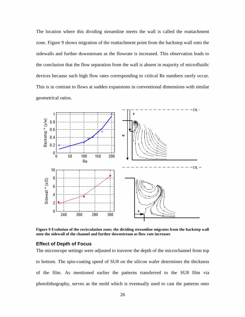
The location where this dividing streamline meets the wall is called the reattachment

zone. Figure 9 shows migration of the reattachment point from the backstep wall onto the

sidewalls and further downstream as the flowrate is increased. This observation leads to

the conclusion that the flow separation from the wall is absent in majority of microfluidic

devices because such high flow rates corresponding to critical Re numbers rarely occur.

This is in contrast to flows at sudden expansions in conventional dimensions with similar

geometrical ratios.

Figure 9 Evolution of the recirculation zone; the dividing streamline migrates from the backstep wall

onto the sidewall of the channel and further downstream as flow rate increases

Effect of Depth of Focus

The microscope settings were adjusted to traverse the depth of the microchannel from top

to bottom. The spin-coating speed of SU8 on the silicon wafer determines the thickness

of the film. As mentioned earlier the patterns transferred to the SU8 film via

photolithography, serves as the mold which is eventually used to cast the patterns onto

y CL

w

CL

x

27

the PDMS resin to form the microchannels. The device height in this study was in the

range of 100 to 120 μm; height variation is due to variations in the fabrication process

such as spin coating. The tracer particles used for μPIV were dispersed homogenously in

water and fed into the devices using an infusion pump. The same mixture with identical

tracer particle concentration was used for all the test cases. The size of the tracer particles

(1μm on average) is much smaller than typical dimensions of the flow such as the width

and height of the device which ensures that the particles would follow the flow

reasonably well. The border of the channels, as observed through the microscope,

consists of a line with two edges; each representing the intersection of the sidewall with

the top and the bottom wall. By adjusting the objective lens to be focused on the upper or

lower bounds of the channel, one of those two lines would appear sharp and the other

blurry (sidewall is not perfectly vertical). In this way, it is possible to pinpoint the upper

and lower walls and calibrate the markings on the microscope focusing knobs with the

actual microchannel depth. In (Figure 10), a series of PIV realizations are shown which

correspond to various depths from the top to bottom of the microchannel. It is observed

that given a preset time-interval (Δt=100μs) and flow rate, the resulting images from the

correlation algorithm show almost the same flow pattern. This is an important finding

since we explained earlier that with regards to the dimensions of the device, the top and

bottom walls would certainly affect the flow field and that the flow is a function of the

depth coordinate (3D flow).

28

Figure 10 μPIV realizations of a recirculation flow at various depths of focus from top to bottom of

the device; (Z*=z/H, D100μsec, Re=222); variation of depth of focus has insignificant effect on the

output flow profile.

expansion_HundredFourtyThree00056.vec

Frame 001 21 Dec 2008 C:Experimentsexpansion_HundredFourtyThreeVectorConditionedexpansion_HundredFourtyThree00056.vec

expansion_HundredFourtyFour00056.vec

Frame 001 21 Dec 2008 C:Experimentsexpansion_HundredFourtyFourVectorConditionedexpansion_HundredFourtyFour00056.vec

expansion_HundredFourtySeven00056.vec

Frame 001 21 Dec 2008 C:Experimentsexpansion_HundredFourtySevenVectorConditionedexpansion_HundredFourtySeven00056.ve

expansion_HundredFourtyTwo00056.vec

Frame 001 21 Dec 2008 C:Experimentsexpansion_HundredFourtyTwoVectorConditionedexpansion_HundredFourtyTwo00056.vec

Z*= 0.16 Z*= 0.33

Z*= 0.5 Z*= 0.83

29

It was observed that except for a slight change in the resolution and overall quality of the

images, the recorded flow fields are identical at various depth-of-focus values. This leads

to the conclusion that the ―ensemble cross correlation algorithm‖ is less sensitive to the

depth of focus. if not so, then the flow patterns resulting from using different values of

depth-of-focus should have been different.

Effect of Time Interval between PIV Image-Pairs

In order to investigate the effect of time intervals (Δt) between PIV recordings of image-

pairs, the depth of focus, flow rate and other parameters were set as constants and various

time intervals were chosen. The µPIV results for a given flow rate and depth are expected

to have a steady flow pattern regardless of imaging time interval at least qualitatively.

From (Figure 11), it can be concluded that the cross correlation algorithm is highly

sensitive to the time interval used for PIV recording of image-pairs. It was observed that

depending on the value chosen for the time interval, the algorithm gets locked into a

plane of flow that can be resolved within the range of parameters chosen, and which

results in the most frequently occurring displacement peaks over the averaged image-

pairs, regardless of the depth of focus. Note that the flow rate and depth of focus are held

constant and at least qualitatively similar flow patterns should have been observed using

a constant flow rate and depth-of-focus. However, the flow fields resulting from the three

cases are significantly different in terms of qualitative flow patterns as well as

quantitative values of the velocity magnitudes. Layers of fluid moving closer to the top

and bottom walls have lower velocity magnitudes compared to those close to the center

of the channel due to the no slip condition; larger time intervals are required to resolve

30

slow moving layers while for the faster moving layers at the core of the flow, shorter time

intervals should be used.

Figure 11 μPIV realizations using different values of time interval (Dt) between recordings of the PIV

image pairs; depth of focus (Z*=0.5) and flow rate (Re=222) were held constant. Resulting flow

patterns differ qualitatively and quantitatively.

Vel Mag

0.048

0.038

0.029

0.019

0.010

0.000

expansion_twentyNine00061.vec

Frame 001 21 Dec 2008 E:EHSANLAB270Experimentsexpansion_twentyNineVectorConditionedexpansion_twentyNine00061.vec

Vel Mag

0.022

0.018

0.013

0.009

0.004

0.000

expansion_thirtySeven00055.vec

Frame 001 21 Dec 2008 E:EHSANLAB270Experimentsexpansion_thirtySevenVectorConditionedexpansion_thirtySeven00055.vec

Vel Mag

0.018

0.014

0.011

0.007

0.004

0.000

expansion_thirtyTwo00055.vec

Frame 001 21 Dec 2008 E:EHSANLAB270Experimentsexpansion_thirtyTwoVectorConditionedexpansion_thirtyTwo00055.vec

Δt = 200 μs

Δt = 400 μs

Δt = 500 μs

31

In this sense, there can be an indirect correlation between the depth at which the flow

field is computed and the time interval used to record that flow field.

Conclusion

Backward facing step flow was visualized in a 1:5 expansion ratio in a microchannel

using the μPIV technique. The device was fabricated using the well established SU8

lithography and PDMS soft lithography fabrication process. Three variables were

investigated while making flow visualizations. First, the flow rate was increased in

increments to find out the onset of vortex generation and emergence of flow recirculation

zones. The behavior of the vortex in a given plane of flow was investigated and migration

of the dividing streamline was observed; the dividing streamline initially resides on the

backstep wall and gradually shifts on to the sidewall and moves downstream as the flow

rate is further increased. It was concluded that the flow hardly gets separated from the

wall in normal flow rates used in microfluidic devices even with geometrically favorable

features for recirculation and separation to occur. The onset of recirculation was observed

at relatively large flow rates. This reconfirms that the fluid flows are highly ordered and

laminar at reduced scales and cannot be disrupted easily. Second, the effect of depth of

focus was studied on the μPIV visualizations. It was observed that the cross-correlation

algorithm used in this study (ensemble cross correlation) was not sensitive to the exact

focusing of the optics on a given plane of flow as long as long as the focus remained

within the upper and lower bounds of the microchannel. Finally, it was observed that the

algorithm is highly affected by the value of time intervals used for recording PIV double

image-pairs. In other words, with a given time interval, only that portion of the flow

which yields the most repeated displacement peaks in the interrogation spots is resolved

32

as the final output. By considering a set of μPIV realizations using incremental time

intervals and combining them together, an indirect method for resolving the depth

coordinate of the flow (often a challenging subject) in μPIV realization using ensemble

cross correlation schemes.

33

List of References

Armaly, B. F., F. Durst, et al. (1983). "Experimental and theoretical investigation of

backward-facing step flow." Journal of Fluid Mechanics 127: 473-496.

Biswas, G., M. Breuer, et al. (2004). "Backward-Facing Step Flows for Various

Expansion Ratios at Low and Moderate Reynolds Numbers." Journal of Fluids

Engineering 126(3): 362-374.

Bourdon, C. J., M. G. Olsen, et al. (2004). "Power-filter technique for modifying depth of

correlation in microPIV experiments." Experiments in Fluids 37(2): 263-271.

Carl, D. M., T. W. Steve, et al. (2000). "A PIV Algorithm for Estimating Time-Averaged

Velocity Fields." Journal of Fluids Engineering 122(2): 285-289.

Devasenathipathy, S., J. G. Santiago, et al. (2002). "Particle Tracking Techniques for

Electrokinetic Microchannel Flows." Anal. Chem. 74(15): 3704-3713.

Gad-el-Hak, M. (2005). The MEMS Handbook, CRC Press.

Jo, B.-H., L. M. Van Lerberghe, et al. (2000). "Three-dimensional micro-channel

fabrication in polydimethylsiloxane(PDMS) elastomer." Journal of

Microelectromechanical Systems 9(1): 76-81.

Meinhart, C. D., S. T. Wereley, et al. (2000). "Volume illumination for two-dimensional

particle image velocimetry." Measurement Science and Technology(6): 809.

Meinhart, C. D., S. T. Wereley, et al. (1998). Micron-resolution velocimetry techniques.

Developments in laser techniques and applications to fluid mechanics. R. J. A. e. al.

Berlin, Springer Verlag.

Nguyen, N.-T. and S. T. Wereley (2002). Fundamentals and applications of

microfluidics, Artech House.

34

Olsen, M. G. and R. J. Adrian (2000). "Brownian motion and correlation in particle

image velocimetry." Optics & Laser Technology 32(7-8): 621-627.

Olsen, M. G. and R. J. Adrian (2000). "Out-of-focus effects on particle image visibility

and correlation in microscopic particle image velocimetry." Experiments in Fluids 29(7):

S166-S174.

Santiago, J. G., S. T. Wereley, et al. (1998). "A particle image velocimetry system for

microfluidics." Experiments in Fluids 25(4): 316-319.

35

CHAPTER TWO: DESIGN, FABRICATION AND CHARACTERIZATION OF AN IN-PLANE PASSIVE MICROMIXER

Introduction

Microfluidics is an enabling technology that allows fluids to be processed in smaller

volumes and on faster time scales (Floyd-Smith, Golden et al. 2006). Microfluidic

channels need much smaller volumes of biochemical reactants than analyzers in

traditional technology and their performance is more efficient due to their enhanced heat

and mass transfer properties. Another advantage is the precise controllability of flow by

applying electric fields, pressure gradient, geometry design of the channel or by a

combination of these methods (Niu and Lee 2003). Microfluidic devices are mainly

targeted towards chemical and biological applications where rapid and efficient mixing is

essential. Mixing is of considerable importance to realizing lab-on-a-chip (LOC) bio-

analysis systems since a majority of the applications often involve reactions that require

quick and efficient mixing of reactants for initiation (Liu, Stremler et al. 2000).

Nevertheless, mixing is greatly limited at the microscale where fluid flow is almost in all

cases laminar. In laminar flows, layers of fluid co-flow and slide over their neighboring

layers in a parallel manner without significant motion in the transverse direction.

The generic transport equation of any scalar υ (temperature in heat transfer, velocity in

momentum and concentration in mass transfer) is given as follows:

Sut

).().( 4

ρ, u and Γ are the density, velocity and diffusion constant respectively and Sυ is the

source term. In a steady state situation with no sink or source terms, the transport

phenomenon is governed by diffusion-based and convective-based effects represented by

36

the first term on the right hand side and second term on the left hand side of the equation

respectively.

Flow in microdevices is usually characterized by low Reynolds numbers (Re =ρVd/μ=

0.01 – 10) because the inertial effects are very small compared to viscosity related ones.

(ρ, V and μ are density, average velocity, and viscosity of the fluid and d is a

characteristic length of the system). Therefore, transport processes at the microscale are

mainly due to the random motion of the molecules, i. e., diffusion-based processes.

Accordingly, the dominating process in micromixing (mass transport) is also based on

molecular diffusion, which is relatively slow. Furthermore, values of the Peclet number

are relatively high in microchannels (Pe = Vd/Dmol > 100, where Dmol, is the molecular

diffusivity), indicating that diffusive mixing occurs at slower rates compared to the

timescales associated with fluid motion (Sudarsan and Ugaz 2006). The diffusive mass-

flux across an interface of miscible media is proportional to the interfacial area and

concentration gradient between the two. Since both the linear proportionality factor of

diffusion (the diffusion constant, Dmol) and the concentration gradient are constants in

most cases, one strategy to enhance the mixing is to maximize interfacial surfaces

between the fluids. However, the maximum possible interfacial area generation is related

to the viscous dissipation. Thus, efficient mixing and viscous dissipation, i.e., energy

consumption, are inevitably interlinked (Hessel, Löwe et al. 2005).

In the low Reynolds number, common methods of mixing used at the macroscale based

on inertial or convective processes, such as creating chaotic and turbulent motion, in

order to promote mixing, are less likely to be effective. However, some researchers have

proposed solutions using inertial effects. Liu et al. proposed an alternative approach to

37

induce chaotic advections to perturb the lamellae of fluid and increase mixing (Liu,

Stremler et al. 2000) . This is achieved by different means such as development of

secondary flows inherent to 3D flow geometries. Although the key advantage of the

chaotic-advection based strategies is that an exponential rate of mixing is achieved, as

opposed to an algebraic rate (e.g. t-1

), the structure becomes geometrically complex

(Bottausci, Cardonne et al. 2006).

In order to overcome viscous opposition to fluid flow, energy is required to flow the

fluid. Micromixers are categorized based on how this energy is provided to the device.

The mixing relies either on the pumping energy or provision of other external energy to

achieve mixing, termed as passive and active mixing, respectively. Compared with active

mixers, passive mixers have the advantages of low cost, ease of fabrication and

integration within microfluidic systems and no complex control units being involved

since there are no moving parts; in addition passive mixers do not need additional power

input. Therefore, passive mixers and typical microstructured flow mixing designs are

favorable for single-use disposable units in biological and chemical microsystems.

(Hong, Choi et al. 2004). Hessel et al (Hessel, Löwe et al. 2005) published a

comprehensive review in which different concepts and designs of micromixers are

explained. Serpentine Structure (Liu, Stremler et al. 2000), Modified Tesla Structure

(Hong, Choi et al. 2004), Split and Recombine Structure (SAR) (Schonfeld, Hessel et al.

2004) and Chaotic Flow Configuration (Stroock, Dertinger et al. 2002) micromixers are

examples of passive mixing devices proposed by researchers in recent years. Although

the micromixing problem has been studied widely, there still exists technical challenges

related to the performance, fabrication and integration of micromixers.

38

Here, the effect of the laminar velocity profile on the diffusive mixing is studied and a

novel and highly efficient yet very simple design of a passive micromixer which takes

advantage of variable inter-lamellae interface velocity is proposed. It was found that

mixing performance is highly enhanced if diffusion interfaces between miscible streams

attain the highest velocity possible throughout the residence time of fluids in the mixer,

given the flow rate, critical dimensions and other design constraints. Experimental

observations and numerical simulation results are provided to support the solution

proposed to enhance passive micromixing. Based on the idea presented, a 2-D in plane

passive micromixer was designed, fabricated and its functionality tested. Furthermore,

the idea of achieving variable velocity profile in laminar flow of the proposed mixing

scheme is confirmed with the aid of micro Particle Image Velocimetry (μPIV).

Methods and Materials

Theory

In order to explain the micromixing strategy, a simplified theoretical model of the

problem is introduced. Consider a film of liquid B, with a given (parabolic) velocity

profile, where species A diffuses in from a constant-concentration source (Figure 12).

This is a simplifying assumption and actually when two streams inter-diffuse,

concentration of species vary but are conserved quantities along the mixing path. The

mass diffusion of A inside B is a classic mass transfer problem (Bird, Stewart et al.

2007). It is assumed that diffusion of species would not alter the hydrodynamics of the

laminar flow (the viscosity and velocity profile). Another restriction imposed on the

problem is that, diffusion takes place slow enough that the diffused species would not

penetrate very far into the liquid.

39

Figure 12 Diffusion of species A into liquid film B; C0A is the solubility limit of A in to liquid B

The velocity profile has a general form of:

])(1[ 2

maxxvvz

5

where, x=0 is at the interface, vz, vmax, δ are velocity, maximum velocity and film

thickness respectively. Using the transport for diffusion of species A, and considering the

fact that mass transfer is predominantly diffusion based in the transverse direction, x

(convective term neglected in x) and convection based in the motion direction, z

(diffusive term neglected in z), the governing differential equation for concentration

distribution of species A, cA is given as follows with DA,B as the binary diffusion

constant:

2

2

,x

cD

z

cv A

BAA

z

6

Substitution of Eq. (5) in Eq. (6) gives

2

2

,

2

max ])(1[x

cD

z

cxv ABA

A

7

With the following boundary conditions:

z=0 cA=0

x=0 cA=cA0

x=δ ∂c/∂x=0

The solution to this problem is in the form of a series given by P.L. Pigford (1941);

however, a limiting expression for small values of δ/vmax is given.

B

A

Vmax z

x

C0A

δ

40

Considering the restriction set before, that species A does not penetrate a long distance

compared to the thickness of the liquid film, one can argue that species A would observe

the liquid film B, to be moving in z direction with a velocity equal to vmax. In other

words, since A diffuses to a depth very close to the interface, it does not sense the

presence of the solid wall at x=δ, hence the variations of the velocity from the interface

into depth and towards the wall. Based on this restriction, the current problem can be

approximated as a problem of diffusion of A into an infinite thickness layer of liquid

moving with the velocity vmax. Then, the simplified governing equation becomes:

2

2

,maxx

cD

z

cv A

BAA

8

By using a similarity variable approach, the solution has the following form:

)/4

()exp(2

1max.

/4/

0

2

0

max,

vzD

xerfcd

c

c

BA

vzDx

A

A

BA

9

Once the concentration gradients are known, the local mass flux at the interface may be

found as follows:

z

vDc

x

cDzN

BA

Ax

ABAxA

max,

00

,interface,, )( 10

It is observed that if the mass flux - diffusion of species A into B - is to be increased, then

one way is to have the highest possible value of vmax at the interface of the two miscible

fluids since it appears in the numerator of the flux term and increase in vmax will lead to

increase in the mass flux at the interface. This relationship is a key point for the design of

the proposed micromixer.

Looking into the original mixing problem in a micromixer where two streams of miscible

liquids, A and B, flowing side by side in a laminar regime in a microchannel, there would

be two diffusion fronts developed which progress in the transverse direction of the flow

41

as one proceeds from the beginning to the end of the channel. It is expected based on the

above mentioned, if velocities at the interfaces of the two fluids were increased, the

diffusive flux would increase. However, as the two fluids mix, the interfaces would shift

away from the centerline as one moves downstream of the channel, i.e., in the increasing

z-direction (Figure 13).

Figure 13 Progression of diffusion interfaces in the transverse direction to the flow; two interfaces

are developed and move away from the centerline of the channel as one moves downstream

Based on Einstein’s relationship for Brownian motion, it can be shown that the position

of the diffusion interface of each of the species (fronts) would progress from the initial

location (centerline) in the x-direction (in both ways) as follows:

21

,2

1

, )2()2()(U

zDDzx BABA

11

x, τ and Ū are, displacement of interface from centerline, channel residence time and

average fluid velocity respectively.

The two key facts of this work are established as follows:

(1) Mass flux at the interface of species diffusing into a liquid film from a constant source

increases as interface-velocity is increased;

(2) Interfaces progress in the transverse direction(x) as we go downstream the channel,

Based on these two facts, novel passive mixer design is proposed that takes advantage of

flow profile variation. The sidewalls cause the flow profile to change in such a way that

the maximum (vmax) is not always in the center line and gets shifted periodically across

42

the transverse direction. Due to the repeating patterns the shift in maximum velocity

occurs periodically where the progressing diffusion fronts and the maximum velocity

coincide repeatedly during the residence time of the fluid inside the mixing channel. This

is in contrast to the conventional T mixer that has a constant parabolic velocity profile,

where the maximum occurs only at the centerline (Figure 13). With respect to the

established facts, coincidence of diffusion interfaces with fast moving layers of fluid

result in better mass transfer, hence better diffusive mixing. It should be noted that in a

microchannel the velocity profile is also dependent on the depth of channel, y coordinate,

where as here a 2D configuration was assumed for the velocity that is independent of y;

this would not hurt the argument, since it can be said that the result is true at any given y

(depth in the microchannel). Velocity, vz-, would vary along x in the form of a parabolic

profile but with different magnitudes depending on y. Detailed study of the effect of the

velocity profile and the near wall effects has been performed by Kamholz (Kamholz and

Yager 2001) and Ismagilov (Ismagilov, Stroock et al. 2000) where a so called Butterfly

effect has been detected and explained at the cross-section of microchannel with binary

diffusion taking place.

In summary, altering the velocity profile repeatedly throughout the mixing channel of the

micromixer tends to increase the mixing performance. The next step is to develop the

desired velocity profile which would have its maximum value vary across the transverse

direction, x, as a function of the motion wise coordinate, z in a passive manner. This has

been accomplished by the design of the sidewalls. In this way not only the maximum of

the velocity profile shifts in the transverse direction periodically throughout the channel

but also, the overall interfacial area between the two streams is increased which also has a

43

positive effect on the mixing performance. Each layer of fluid undergoes acceleration and

deceleration passing through the mixer and the maximum velocities coincides with the

progressing diffusion fronts more often on average and with regards to the established

key points developed in this study, diffusive mass flux increases across these interfaces,

hence increasing the mixing efficiency of the micromixer. Schematic of the sidewall

profile and how the velocity profile is affected passively is illustrated in (Figure 14).

Figure 14 Velocity profile, unlike in a T-mixer, varies throughout the channel passively and

periodically due to the sidewall design; sidewall profiles expand and contract asymmetrically

(descending slope is steeper than the ascending slope). The velocity profile maximum, shifts

transversely such that it coincides with the diffusion interfaces repeatedly. Increased velocity at

interfaces, results in enhance flux of species.

Alternating acceleration and deceleration of the layers relative to each other lead to high

mixing efficiency without resorting to complex features that create stagnation or

recirculation of the fluid which leads to trap zones and dead volumes. As shown in

(Figure 14), parameters a and b define the ellipsoid used to generate the side wall

patterns. They are chosen such that, asymmetric sidewalls are generated with least

parallelism and that the maximum variation of the velocity profile is achieved passively.

λ is the periodic length of the repeating sidewall profiles. H is predefined as channel

width and h is the constriction width that together with other parameters makes the

sidewalls expand or contract asymmetrically; if chosen too small, then large pressure

H

b

a

R1

λ

R2

hH

b

a

R1

λ

R2

h

44

drops would occur. Sharp corners are removed by making the walls smooth to ensure that

no dead volumes are created in the device (R). Numerical simulations resulted in

optimized values of H=200, h=50, a=300, b=100, R=100 λ=400 and with channel depth

of 100 (unit: micrometer).

Numerical Simulation

Numerical simulation results are presented to show the effect of velocity profile variation

on promoting the diffusive mixing. Velocity profiles extracted at two corresponding

cross-sections are shown in (Figure 15) shows the change in velocity profile and the

shifting of the maximum from the center towards the side walls from upstream to

downstream of the channel in a repeating cell. This shift takes place periodically

throughout the channel; hence the interface layers experience a variable velocity in

contrast to the case of a straight channel with fixed velocity profile.

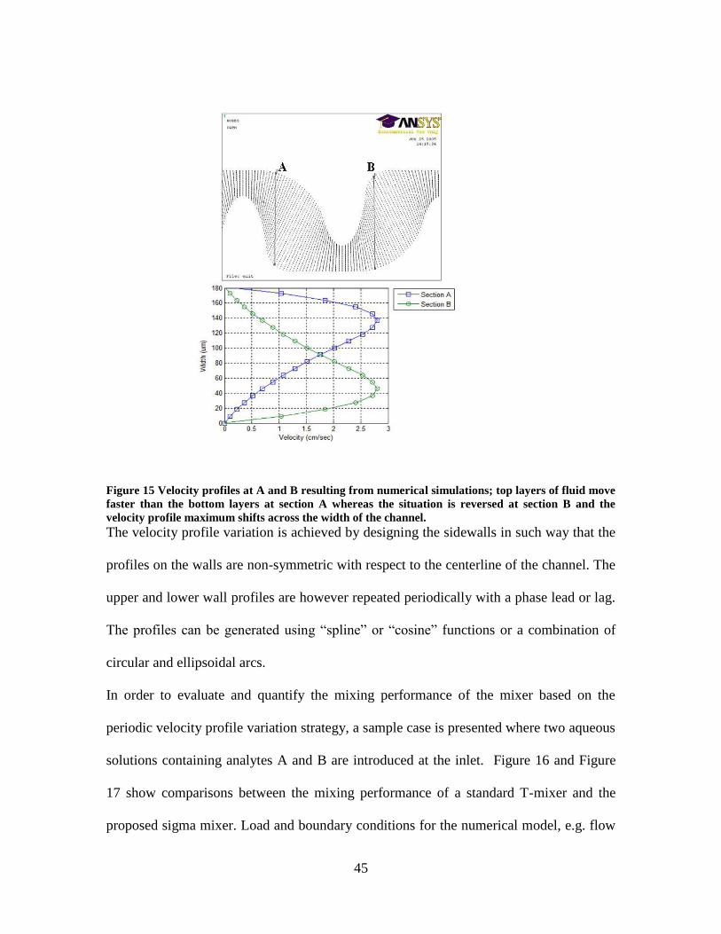
45

Figure 15 Velocity profiles at A and B resulting from numerical simulations; top layers of fluid move

faster than the bottom layers at section A whereas the situation is reversed at section B and the

velocity profile maximum shifts across the width of the channel.

The velocity profile variation is achieved by designing the sidewalls in such way that the

profiles on the walls are non-symmetric with respect to the centerline of the channel. The

upper and lower wall profiles are however repeated periodically with a phase lead or lag.

The profiles can be generated using ―spline‖ or ―cosine‖ functions or a combination of

circular and ellipsoidal arcs.

In order to evaluate and quantify the mixing performance of the mixer based on the

periodic velocity profile variation strategy, a sample case is presented where two aqueous

solutions containing analytes A and B are introduced at the inlet. Figure 16 and Figure

17 show comparisons between the mixing performance of a standard T-mixer and the

proposed sigma mixer. Load and boundary conditions for the numerical model, e.g. flow

46

rate, inlet concentration profiles and outlet pressure are chosen such that the governing

parameters like the Reynolds (UDH/ν) and Peclet number (UDH/DA,B) are identical in

order for the results to be comparable. The hydraulic diameter is taken to be similar too.

(DH=4A/P where A and P are the inlet cross section area and the wetted perimeter of the

channels respectively, U is the average velocity and ν is the kinematic viscosity of the

solution). Results are given for a case where Reynolds and Peclet number are 1.65 and

730 respectively. The ideal situation is to have an even distribution of both analyte

concentration over the cross-section of the outlet (both analytes having a constant

concentration across the width, in this case C* of 0.5). The mixing efficiency is defined

as follows:

N

j j ccN 1

21

2 ]*)(1

[ 12

cj is the concentration of cross section nodes and j is the index; The mixing efficiency

(%) is defined as :

%100)5.0(%M 13

σ has the form of standard deviation; standard deviation (STD) of the concentration

distribution of each analyte over the channel width can be calculated and used as a

measure of mixing performance. The lower the deviation from the average value, the

better mixing has occurred. Perfect mixing is when the STD goes to zero and an average

concentration of C*=0.5 is achieved all over the cross section. As can be seen in (Figure

17) both mixers show similar decrease in mixing performance with increased average

flow speed, confirming diffusion dominated mixing mechanism in the highly laminar

regime; however, the modified sigma micromixer show superior mixing performance at a

given working flow rate.

47

Figure 16 Contour plots of concentration comparing mixing performance of the standard T mixer

and the Modified Sigma micromixer. Ideally, at the exit all cross section elements should attain a

relative concentration of C*=0.5 showing perfect dispersion of one species in another.

Figure 17 Mixing performance deteriorates for mixers as inlet velocity increases confirming the

diffusion-based nature of mixing in microdevices (U*=Umax_inlet / [μ/ρ.Dh] ~ Remax, μ=0.001Pa.sec,

ρ=1000kg.m-3

and Dh=100μm)

In conclusion, numerical results supported the idea that the higher the velocity profile

variation is along the mixer length, the better the mixing performance would be. In

addition to numerical results, the variation of laminar velocity profile was confirmed

using micro Particle Image Velocimetry technique (Figure 18).

48

Figure 18 Actual μPIV flow visualization inside the micromixer; top layers at section A move slower

than the bottom layers of the fluid where as the situation is reversed in section B. (note the shifting of

the velocity profile maximum across the width from A to B)

Fabrication

The proposed micromixer has a 2-D in-plane structure which makes the fabrication and

integration convenient. Mixing is achieved without resorting to any complex geometry

unlike devices proposed in other designs (Liu, Stremler et al. 2000; Stroock, Dertinger et

al. 2002; Jen, Wu et al. 2003; Schonfeld, Hessel et al. 2004). Considering the

applications, which can range from one-time use disposable assay chips to integrated

49

microfluidic platforms for combinatorial chemistry testing devices used in

pharmaceutical research, emphasis has been placed on having the simplest yet effective

structures of all. In addition, unlike active micromixers, where an external source of

energy is required to promote the mixing, the proposed design falls into the category of

passive devices which can easily be integrated into any microscale platform and function

on a stand alone basis.

A typical procedure of fabricating a microchannel is to spin coat a layer photoresist on a

substrate; the thickness of the coating would determine the height of the microchannels.

Patterning the photoresist via photolithography is used to make a mold which will

eventually be used to replicate channels in an elastomer (Poly-dimethyl-siloxane PDMS).

The elastomer which comes in liquid form is mixed with a curing agent and poured on

mold and allowed to cure. The PDMS layer consisting of transferred patternes

(microchannels) is bonded to another blank layer of PDMS or glass slide to create a

closed fluidic channel by surface treatment. Inlet and outlet ports would be punched in

the blank layers (Figure 19).

50

Figure 19 General procedure for making microchannel using the SU8 resist and PDMS replication

SU-8 is a high-contrast, epoxy based negative photoresist used for micromachining and

other microelectronic and microfluidic applications, where thick, chemically and

thermally stable features are desired. Film thicknesses in the range 0.5 to less than 200

micrometers can be achieved with a single coat process. The exposed and subsequently

thermally cross-linked portions of the film are rendered insoluble to liquid developers

(Appendix 1). SU-8 is used to create high aspect ratio structures with near vertical walls

in very thick films due to its optical properties. In (Figure 20), scanning electron

microscopy image of the fabricated devices is shown.

51

Figure 20 Scanning Electron Microscopy (SEM) images of a) oblique view of the micromixer

channel, b) rectangular cross-section of the channel c) smooth surface of the micromixng walls d)

intersection of channel with the reservoir

Results - Characterization

In order to observe the efficiency of the proposed micromixer, an accepted method

proposed for mixing evaluation is adopted. An experiment was setup where two streams,

a base solution (sodium hydroxide) and a pH indicator solution (phenolphthalein) are

pumped into the mixer. Upon mixing the transparent solution will turn into pink/purple

color (Liu, Stremler et al. 2000)). Phenolphetalein and sodium hydroxide solution are

both colorless but once mixed turn into a dark pink/ purple color.

Phenolphthalein solution (phenolphthalein 1 %, isopropyl alcohol 60 %, water balance)

and 0.4N sodium hydroxide solution (1.6 % sodium hydroxide in a similar solution to

above and pH=12.5) were used. The two colorless solutions are introduced at the inlets of

52

the devices by an infusion pump. When mixed, a pink/purple region is created which

expands transversely with two interfaces away from the centerline as the solutions further

mix downstream. Color images (Lee, Kim et al. 2006) at select cross sections are

converted into gray-scale images. Pixels with gray intensity I=0, show fully mixed

regions whereas bright pixels, I=1, are non-mixed portions of the flow (Figure 21). The

deviation of gray intensity around the darkest gray pixel (completely mixed region in the

middle of the channel) is calculated for the pixels of the selected cross section (Stroock,

Dertinger et al. 2002).

n

i

iIIn 1

21

2

min ])(1

[

14

n is the number of the cross section pixels, Ii is gray intensity of pixel i of the selected

cross section and Imin is the minimum gray intensity. When there is no mixing, the

standard deviation, σ=1, and ideally at full mixing it will reach 0 as all pixels attain

uniform gray intensity (Appendix 2).

Figure 21 Evaluation of mixing performance using color changes as a result of mixing of a pH

indicator (phenolphthalein) and a base solution (sodium hydroxide, pH=12.5) Performance of

Modified Sigma and the Standard T mixers at 3mm mixing length; the wider the gray region, the

better the solutions have mixed( Re=0.4, Q=350μl.hr-1

, Dhydraulic = 66μm)

53

The level of mixing (percentage) is defined as follows:

100)1((%)M 15

The mixing performance was evaluated in comparison to the T mixer and the Modified

Tesla Structure mixer as a function flow Reynolds number and mixing length (Figure 22).

The result validates the effectiveness of the proposed passive micromixing concept and

improvement of mixing performance. In addition to having the advantage of no-dead

volume, the sigma mixer achieves satisfactory mixing in smaller mixing lengths; hence

favorable option for limited size chips and platforms.

54

Figure 22 Mixing performance at a given mixing length (L=8 mm) as a function of flow Reynolds

number, b) Mixing performance at a given flow rate (Q=1000 μl/hr, Re=0.91) as a function of mixing

length.

55

Conclusion

In this study, it was demonstrated that the diffusive mass flux between streams of fluid

flowing in a laminar regime increases as the velocity of the interface between the streams

of liquid increases; Since, the interfaces progress in the transverse direction as one moves

downstream the flow, by causing the maximum of the velocity profile to be shifted from

the centerline to coincide with the moving interfaces as often as possible, significant

improvement in mixing can be expected. A novel micromixer concept has been proposed

based on this idea. Numerical simulation was performed and based on the results, a 2-D

in-plane micromixer was fabricated and its functionality verified by color analysis due to

mixing of phenophetalein (pH indicator) and sodium hydroxide (pH=12). The proposed

micromixer can be adopted to a wide-range of microfluidic applications in the low

Reynolds number flows. The simple yet effective design facilitates the fabrication and

integration of the proposed micromixer which is favorable for disposable polymer-based

biochemical assay chips. The micromixer is passive thus energy efficient and is expected

to be compatible with various pumping mechanisms including capillary, hydraulic, and

electrokinetic systems. Finally, the device has no dead volumes or recirculation zones,

causing otherwise incomplete homogenization or cross-contamination of reagents. The

proposed device can be fabricated and integrated with a single mask photolithography

very easily due to its in-plane structure, making it superior and more favorable for mass

produced disposable micro-fluidic platforms.

56

List of References

Bird, R. B., W. E. Stewart, et al. (2007). Transpot Phenomenon. New York, J. Wiley.

Bottausci, F., C. Cardonne, et al. (2006). "An Actively Controlled Micromixer: 3-D

Aspect." Microfluidics: History, Theory and Applications.

Floyd-Smith, T. M., J. P. Golden, et al. (2006). "Characterization of passive microfluidic

mixers fabricated using soft lithography." Microfluid Nanofluid 2: 180-183.

Hessel, V., H. Löwe, et al. (2005). "Micromixers—a review on passive and active mixing

principles." Chemical Engineering Science 60: 2479-2501.

Hong, C.-C., J.-W. Choi, et al. (2004). "A novel in-plane passive microfluidic mixer with

modified Tesla structures." Lab Chip 4: 109-113.

Hong, C. C., J. W. Choi, et al. (2004). "A novel in-plane passive microfluidic mixer with

modified Tesla structures." Lab Chip 4: 109-113.

Ismagilov, R. F., A. D. Stroock, et al. (2000). "Experimental and theoretical scaling laws

for transverse diffusive broadening in two-phase laminar flows in microchannels."

Applied Physics Letters 76(17): 2376-2378.

Jen, C. P., C. Y. Wu, et al. (2003). "Design and simulation of the micromixer with

chaotic advection in twisted microchannels." Lab Chip 3: 77-81.

Kamholz, A. E. and P. Yager (2001). "Theoretical analysis of molecular diffusion in

pressure-driven laminar flow in microfluidic channels." Biophysical Journal 80: 155-160.

Lee, S. W., D. S. Kim, et al. (2006). "A split and recombination micromixer fabricated in

a PDMS three-dimensional structure." Journal of Micromechanics and Microengineering

16(5): 1067-1072.

57

Liu, R. H., M. A. Stremler, et al. (2000). "Passive Mixing in a Three-Dimensional

Serpentine Microchannel." Journal of Microelectromechanical Systems 9: 190-197.

Niu, X. and Y.-K. Lee (2003). "Efficient spatial-temporal chaotic mixing in

microchannels." Journal of Micromechanics and Microengineering(13): 454-462.

Schonfeld, F., V. Hessel, et al. (2004). "An optimised split-and-recombine micro-mixer

with uniform chaotic mixing." Lab Chip 4: 65-69.

Stroock, A. D., S. K. W. Dertinger, et al. (2002). "Chaotic Mixer for Microchannels."

Science 295(25): 647-651.

Stroock, A. D., S. K. W. Dertinger, et al. (2002). "Chaotic Mixer for Microchannels."

Science 295(5555): 647-651.

Sudarsan, A. P. and V. M. Ugaz (2006). "Fluid mixing in planar spiral microchannels."

Lab on a Chip 74(6): 74-82.

58

APPENDIX A: SU-8 & PDMS PROCESSING – MICROFLUIDIC CHANNEL FABRICATION

59

A typical procedure of fabricating a microchannel is to spin coat a layer photoresist on a

substrate; the thickness of the coating would determine the height of the microchannels.

Patterning the photoresist via photolithography is used to make a mold which will

eventually be used to replicate channels in an elastomer (Poly-dimethyl-siloxane PDMS).

The elastomer which comes in liquid form is mixed with a curing agent and poured on

mold and allowed to cure. The PDMS layer consisting of transferred patternes

(microchannels) is bonded to another blank layer of PDMS or glass slide to create a

closed fluidic channel by surface treatment. Inlet and outlet ports would be punched in

the blank layers.

SU-8 is a high-contrast, epoxy based negative photoresist used for micromachining and

other microelectronic and microfluidic applications, where thick, chemically and

thermally stable features are desired. Film thicknesses in the range 0.5 to less than 200

micrometers can be achieved with a single coat process. The exposed and subsequently

thermally cross-linked portions of the film are rendered insoluble to liquid developers.

SU-8 is used to create high aspect ratio structures with near vertical walls in very thick

films due to its optical properties.

Substrate Preparation

Silicon wafers (mechanical grade) are usually used as base substrates; although other

polished substrates can be used as well. Surface of the substrate needs to be clean, since

the adhesion of SU-8 coating to the substrate is adversely affected by surface

contaminations. Clean the wafer using basic cleaning methods. (For best results,

60

substrates should be cleaned with a piranha wet etch using H2SO4 and H2O2 followed by

DI water rinse). Blow-dry the wafers. After cleaning, place the wafers on 100°C hotplate

for 5 minutes for dehydration.

Coating

SU-8 resists are available in various standards viscosities (this manual is prepared for

SU-8 50 provided by MicroChem® ). For a desired coat thickness, depending on the

viscosity value, appropriate spin-speed should be chosen based on the graphs and tables

provided in manufacturer’s specification sheet.

(a) Apply adequate resist on the substrate (4 ml for 3 inch wafers).

(b) Use a two stage spin coat program as follows ( for film thickness : 100 – 120

μm) :

- 15 seconds @ 500 rpm, acceleration: 85

- 45 seconds @ 1000 rpm, acceleration: 850

(c) Edge bead removal; the resist accumulates on the edges which needs to be

removed using a blade to ensure well-controlled contact with the mask;

otherwise vertical side walls will not be achieved.

Soft Bake

A level hotplate with good thermal control and uniformity is recommended over

convection ovens. Soft bake is performed in a two stages:

(a) 10 minutes on 70°C hotplate

(b) 30 minutes on 105°C hotplate

Allow the wafer to cool down at room temperature before proceeding on to next steps. In

case, wrinkles appear on the surface of the resist, leave the wafer on the hotplate for a

61

few minutes. Repeat the cool-down and heat-up cycle until wrinkles are no longer seen

on the film.

Alignment and Exposure

Follow the instructions given for the EVG aligner to perform the adjustments and

exposure (since a single layer mask is used, alignment is not critical as long as the

features are in bounds of the wafer). SU-8 is optimized for near UV (350-400nm)

exposure. The optimal exposure dose will depend on film thickness (thicker films require

higher dosage) and process parameters.

(a) Follow EVG aligner procedures to load mask and wafer.

(b) Expose for 24 seconds (total dosage for targeted thickness is within 350-400

mJ/cm2)

Adhesion failure, severely negative sidewalls and excessive cracking are often

indications of an under cross-linking condition. To correct the problem, increase your

exposure dose and or increase your post exposure bake (PEB) time.

Post Exposure Bake (PEB)

PEB should take place directly after exposure. PEB is also a two step baking using

hotplates:

(a) 3 minutes on 75°C hotplate

(b) 10 mintues on 105°C hotplate

(c) Allow wafer to cool down to room temperature (thermal shocks will results in form of

cracks or peeling off of the coating if the hot wafers are placed in the developing

solution) After 1 minute of PEB at the higher temperature, an image of the patterns

62

should be visible in the SU-8 coating. If no visible latent image is seen during or after

PEB this means that there was insufficient exposure, heating or both.

Development

SU-8 developer provided by Microchem® is used for developing the patterns (other

solvent based developers such as ethyl lactate and diacentone alcohol may also be used).

Developing time vary largely based on agitation and other factors.

(a) Prepare petri dishes containing SU-8 developer and isopropyl alcohol (IPA).

(b) Recommended developing time is 7 – 10 minutes however, developing time

may be extended (up to 25 minutes). To find out the completion of the

developing process, immerse the wafer into the IPA; if a milky residue is

observed then the development is NOT completed yet.

(c) Once clear patterns emerge and no residue is seen, rinse with IPA and blow

dry using the nitrogen (air) gun.

There is a low risk of over-developing for SU-8; therefore the developing process can be

extended to ensure completion of the process.

Casting – PDMS processing

The fabricated SU-8 mold will be used to replicate patterns in the elastomer resin.

Patterns can be replicated as many times, depending on the quality of the mold. Sylgard

184 Silicone® provided by Dow Corning is used for fabricating the microchannels.

Conventionally, Sylgard 184 is used for microelectronic packaging applications due its

63

robustness, stability and reliability, both mechanical as well as electrical properties. The

two part resin is processed using the following steps:

(a) Place the processed SU-8 mold in a clean petri-dish and tape the edges to the

bottom so it doesn’t move.

(b) Place an empty disposable dish on the laboratory scale and zero the scale

(c) Pour appropriate amount of base resin and curing agent in 10:1 proportion;

usually, 15 grams of base elastomer is sufficient to cover a 3‖wafer and create

a semi-rigid layer; to construct a closed microchannel, two layers are needed)

(d) Stir the mixture thoroughly so that the curing agent and elastomer are

homogenously mixed.

(e) Pour half of the mixture on the wafer that has been tapped to the bottom of the

petri-dish and the remainder in an empty petri dish (to form the blank layer)

(f) Allow the mixture to cure at room temperature. Curing process takes more

that 48 hours. Accelerated curing can also be done using the following

guidelines; however, unwanted bubbles could be trapped during the

accelerated process since curing occurs very fast and there is not enough time

for the degassing of the liquid resin.

35 minutes @ 100°C or 20 minutes @ 125°C or 10 minutes @ 150°C

Ports – Bonding

Once the PDMS layers (blank layer and layer with patterns) are cured, they can be

bonded together to make a closed and leak-free microchannel (Figure 23).

Before bonding, holes are punched in the blank layer using a template. The two surfaces

need to be activated such that when they are brought in contact they would stick

64

permanently. For this purpose, oxygen plasma surface activation can be performed. The

surface modification for PDMS is fairly robust and a handheld Corona plasma generator

is sufficient for the surface treatment.

(a) Place the layers with bonding surfaces facing upwards on the flat disk

shown in (Figure 24). Insert the electrode head in the corona machine

and connect the power supply.

(b) Adjust the height such that the electrode head is 1 cm above the

surfaces.

(c) Remove the samples to tune the plasma arc; there is a tuning knob on

top of the machine which can be used to adjust the arc power. To avoid

sparks, remove any metallic objects (rings, watches and mobile

phones) away from the electrode head. The appropriate arc develops in

the form of a stable blue flame having a buzzing sound. (Too low

voltage on the tuning knob does not develop a flame, while excess

voltage on the other hand, causes sporadic sparks and destabilization of

the flame). Once the tuning is done, turn off the power and replace the

samples on the disk to perform the surface treatment.

65

Figure 23 Two layers of PDMS (top: blank - bottom: with patterns) are bonded to form a closed

microchannel; inlet and outlet ports are punched in the blank layer prior to bonding

Figure 24 Corona surface treatment machine is used to bond pdms-pdms or pdms-glass layers

66

(d) Turn on the power supply and slowly sweep the surfaces under the

flame for surface activation. Treat the surfaces for approximately one

minute each.

After turning off the power, lift the blank layer with a tweezers, minimizing the contacts

with the treated surfaces. Align holes on the blank layer with their counter part reservoirs

on the pattern layer and gently press the two activated surfaces in contact. Apply gentle

pressure on the two layers. Surfaces should be bonded after 5 – 10 minutes.

67

APPENDIX B: IMAGE PROCESSING

68

Introduction

Different methods have been proposed for evaluating the performance and optimizing the

design of micromixers. A common quantification technique is using dilution of a tracer

dye to determine the extent of mixing; for example fluorescent dye and a corresponding

microscope with a filter set are required. The intensity image can then be recorded and

evaluated. Since the concentration of the dye is proportional to the intensity of the

recorded image, the uniformity of the concentration image can be quantified by

determining the standard deviation of the pixel intensity values1 2. Another quantification

method is measuring the fluorescent product of a chemical reaction occurring due to

mixing of two or more reagents introduced to a micromixer 3.

Here we use a characterization method based on color changes resulting from mixing of a

pH indicator solution and a base (pH>7) solution. Phenolphthalein solution

(phenolphthalein 1 %, isopropyl alcohol 60 %, water balance) and 0.4N sodium

hydroxide solution (1.6 % sodium hydroxide in a similar solution to above and pH=12.5)

will be used. The two colorless solutions are introduced at the inlets of the devices by an

infusion pump. When mixed, a pink/purple region is created which expands transversely

with two interfaces away from the centerline as the solutions further mix downstream.

Color images at select cross sections are converted into thresholded grayscale images.

1 Liu R H et al 2000

2 Stroock A D et al 2002

3 Kamholz A E et al 1999

69

Dark pixels, gray intensity I=0, show fully mixed regions whereas bright pixels, I=1, are

non-mixed portions of the flow. Standard deviation of gray intensity around the darkest

gray pixel completely mixed region in the middle of the channel) is calculated for the

pixels of the selected cross section

21

2

1

min ])(1

[ i

n

i

IIn

n is the number of the cross section pixels, Ii is gray intensity of pixel i of the selected

cross section and Imin is the minimum gray intensity. When there is no mixing, the

standard deviation, σ=1, and ideally at full mixing it will reach 0 as all pixels attain

uniform gray intensity. The level of mixing (percentage) is defined as follows:

100)1(%M

The mixing performance is as a function of flow Reynolds number, Peclet number and

mixing length.

DiffLUPe

UDhRe

ρ: fluid density

U: average fluid velocity

Dh: microchannel hydraulic diameter

μ: fluid viscosity

L: mixing length

Diff: diffusion coefficient of liquids

70

At a given flow rate (required flowrate), the shorter the mixing length (L), the better is

the performance of a micromixer. Similarly, when limited mixing length is allowed,

flowrate and channel geometry should be chosen such that appropriate Re and Pe

numbers are achieved to ensure mixing.

Setup

Using an infusion pump, the base solution (pH=12.5) and indicator solution are

introduced to the inlets of the microchannel. A single outlet will be used to extract the

mixed solution out into a beaker. Set the appropriate flow using control keypad on the

infusion pump (Figure 25). Since all physical properties are constant, flowrate can be

changed to achieve various Re numbers.

The micromixer is placed under a microscope equipped with a color digital camera. The

images can be viewed on a computer screen and be saved for image processing.

Figure 25 Infusion pump with control keypad

71

Image Processing

- Initial correction / enhancement using conventional imaging software such as

Microsoft Office Picture Manager.

o Click Edit Pictures Tool → Color→ Enhance Color. Place the crosshair

cursor on a region which is supposed to be clear (white background)

o Choose an appropriate observation window using: Edit Pictures

Tool→Crop. Crop a window equal to the width of the channel and a

length equal to 100 pixels

o Save the resulting image (Figure 26)

Figure 26 Initial image correction / enhancement

- Read the file from previous step in MATLAB using imread command

- Convert the image into grayscale using rgb2gray command

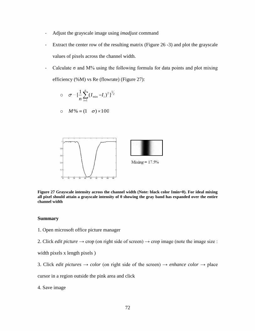
72

- Adjust the grayscale image using imadjust command

- Extract the center row of the resulting matrix (Figure 26 -3) and plot the grayscale

values of pixels across the channel width.

- Calculate σ and M% using the following formula for data points and plot mixing

efficiency (%M) vs Re (flowrate) (Figure 27):

o 21

2

1

min ])(1

[ i

n

i

IIn

o 100)1(%M

Figure 27 Grayscale intensity across the channel width (Note: black color Imin=0). For ideal mixing

all pixel should attain a grayscale intensity of 0 showing the gray band has expanded over the entire

channel width

Summary

1. Open microsoft office picture manager

2. Click edit picture → crop (on right side of screen) → crop image (note the image size :

width pixels x length pixels )

3. Click edit pictures → color (on right side of the screen) → enhance color → place

cursor in a region outside the pink area and click

4. Save image

73

5. read image in matlab : R=imread(‘filename.tif’);

6. convert to grayscale : I= rgb2gray (R);

7. enhance contrast: J= imadjust(I);

8. rescale to range of 0 – 1 : J= double(J)/255;

8. see results: figure, imshow(I), figure, imshow(J),

9. check the size of enhance image: size(J) → [W x L] should be equal to what to noted

in microsoft office picture manager

10. plot the grayscale of a middle column (or row depending on your image orientation)

across the width of the channel: figure, plot(J(:,L/2))

Figure 28 Sequence of steps in image processing for mixing evaluation

74

11. calculate sigma: 21

2

1

min ])(1

[ i

n

i

IIn

and mixing percentage 100)1(%M

For example image size is [79 x 23]:

for i=1:79

SUM=SUM+(J(i,12)-MIN).^2; calculating the

summation

end

SIGMA=sqrt(SUM/79) square root

SIGMA = 0.6949

MIXING=(1-SIGMA)x100