Flight to Quality, Flight to Liquidity,

and the Pricing of Risk

Dimitri Vayanos∗

February 17, 2004

Abstract

We propose a dynamic equilibrium model of a multi-asset market with stochastic volatility

and transaction costs. Our key assumption is that investors are fund managers, subject to

withdrawals when fund performance falls below a threshold. This generates a preference for

liquidity that is time-varying and increasing with volatility. We show that during volatile times,

assets’ liquidity premia increase, investors become more risk averse, assets become more neg-

atively correlated with volatility, assets’ pairwise correlations can increase, and illiquid assets’

market betas increase. Moreover, an unconditional CAPM can understate the risk of illiquid

assets because these assets become riskier when investors are the most risk averse.

∗Sloan School of Management, MIT, Cambridge, MA 02142, email: dimitriv@mit.edu. I thank Viral Acharya,John Cox, Xavier Gabaix, Denis Gromb, Tim Johnson, Leonid Kogan, Pete Kyle, Jonathan Lewellen, Hong Liu,Stew Myers, Jun Pan, Anna Pavlova, Steve Ross, Jiang Wang, Wei Xiong, Jeff Zwiebel, seminar participants atAmsterdam, Athens, Caltech, LSE, LBS, Michigan, MIT, NYU, Princeton, Stockholm, Toulouse, UBC, UCLA, UTAustin, Washington University, and participants at the Econometric Society 2003 Summer Meetings, for helpfulcomments. I am especially grateful to Jeremy Stein for discussions that helped define this project, and for insightfulcomments in later stages. Jiro Kondo provided excellent research assistance. Financial support for this research camefrom the MIT/Merrill Lynch partnership.

1 Introduction

Financial assets differ in their liquidity (i.e., the ease at which they can be transacted), and an

important question is how liquidity affects asset prices. One way to get at this question is to

measure the price differential (liquidity premium) between two assets of different liquidity but very

similar other characteristics. Many examples of such asset pairs come from the government bond

market. Consider, for instance, a just-issued (on-the-run) thirty-year US Treasury bond, and a

thirty-year bond issued three months ago (off-the-run). The two bonds are very similar in terms of

cash flows, but the on-the-run bond is significantly more liquid than its off-the-run counterpart.1

The analysis of liquid/illiquid asset pairs reveals that liquidity premia vary considerably over

time, widening dramatically during extreme market episodes. A term often used to characterize

these episodes is flight to liquidity, suggestive of the notion that investors experience a sudden and

strong preference for holding liquid assets. An example of such an episode is the 1998 financial

crisis. During the crisis, the yield spread between off- and on-the-run thirty-year US Treasury

bonds increased to 24 basis points (bp), from a pre-crisis value of 4bp. Similar increases occurred

in other on-the-run spreads, as well as in other spreads for which liquidity plays some role.2

An important factor driving the variation in liquidity premia seems to be the extent of un-

certainty in the market. For example, during the 1998 crisis there was a dramatic increase in

uncertainty, as measured by the implied volatilities of key financial indices.3 A link between liq-

uidity premia and volatility has also been empirically documented for less extreme times.4

In this paper, we propose an equilibrium model in which (i) assets differ in their liquidity, and

(ii) the extent of uncertainty, represented by the volatility of asset payoffs, is stochastic. Our model

generates liquidity premia that are time-varying and increasing with volatility. Thus, times of high

volatility are associated with a flight to liquidity.1For example, Sundaresan (1997, pp.16-18) reports that trading volume for on-the-run bonds is about ten times

as large as for their off-the-run counterparts. See also Boudoukh and Whitelaw (1991), who document the on-the-runphenomenon in Japan, and Warga (1992), Krishnamurthy (2002), and Goldreich, Hanke, and Nath (2003), who studythe yield spread between off- and on-the-run bonds.

2For example, the on-the-run five-year spread increased from 7bp to 28bp, the ten-year spread from 6bp to 16bp,and the ten-year spread in the UK from 6bp to 18bp. The spread between AA-rated corporate bonds (for whichdefault plays only a minor role) and government bonds increased from 80bp to 150bp in the US, and from 60bpto 120bp in the UK. For more information, and a comprehensive description of the crisis, see the report by theCommittee on the Global Financial System (CGFS (1999)).

3According to CGFS (1999), the implied volatility of the S&P500 index increased from 23% to 43%, that of theFTSE100 index from 27% to 48%, that of the three-month US eurodollar rate from 8% to 33%, and that of thethirty-year US T-bond rate from 7% to 14%.

4For example, Kamara (1994) considers the yield spread between T-notes and T-bills with matched maturities.He shows that the spread (which is mainly due to the notes’ lower liquidity) is correlated with interest-rate volatility.(See also Amihud and Mendelson (1991) and Strebulaev (2003).) Longstaff (2002) considers the yield spread betweenthe securities of Refcorp, a US government agency, and Treasury securities. He shows that the spread (which ismainly due to the lower liquidity of the Refcorp securities) is correlated with a consumer confidence index.

1

In our model, times of high volatility are associated with several other interesting phenomena,

often mentioned in the context of financial crises. We show that during volatile times, investors’

effective risk aversion increases. Thus, there is a flight to quality, in the sense that the risk premium

investors require per unit of volatility increases. We also show that assets become more negatively

correlated with volatility, and can also become more correlated with each other. Moreover, illiquid

assets become riskier, in the sense that their market betas increase. Some of these phenomena

have been documented anecdotally or empirically, and some are new and testable predictions of

our model.5 To our knowledge, our model is the first to show that all these phenomena are related,

and are also related to flight to liquidity.

Finally, our model has the implication that one cost of illiquidity is to make an asset riskier, and

more sensitive to the volatility. We also show that an unconditional CAPM can understate the risk

of illiquid assets because of this risk’s time-varying nature: illiquid assets become riskier in volatile

times, when investors are the most risk averse. This has implications for evaluating the performance

of strategies investing in illiquid assets: if performance is evaluated under an unconditional CAPM,

the strategies could appear better than they actually are.6

We consider a continuous-time, infinite-horizon economy with one riskless and multiple risky

assets. The riskless rate is exogenous and constant over time. The risky assets’ dividend processes

are exogenous, and are characterized by a common volatility parameter which evolves according to

a square-root process. The volatility parameter is the key state variable in our model.

The risky assets differ in their liquidity. To model liquidity, we assume that each asset carries

an exogenous transaction cost. These costs differ across assets, and could arise for reasons outside

the model such as asymmetric information, market-maker inventory costs, search, etc. We assume

that transaction costs are constant over time. Thus, the time-varying liquidity premia arise not

because of the transaction costs, but because of the investors’ willingness to bear these costs.

Our key assumption is in the modelling of investors. We assume that investors are fund man-

agers, managing wealth on behalf of the individuals who own it. Managers receive an exogenous

fee which depends on the amount of wealth under management. They are facing, however, the

probability that the individuals investing in the fund might withdraw their wealth at any time.

Withdrawals occur both for random reasons, and when a fund’s performance falls below an ex-5Section 5 presents the empirical evidence. Anecdotal evidence for increased risk aversion during volatile times

can be found in the CGFS (1999) report. In page 6, the report describes investment decisions at the onset of the1998 crisis as follows: “More fundamentally, investment decisions reflected some combination of an upward revisionto uncertainty surrounding the expected future prices of financial instruments ... and a reduced tolerance for bearingrisk.” The dramatic increases in the yields of speculative-grade corporate bonds and emerging market bonds during thecrisis can also be viewed as evidence for increased risk aversion. Flight-to-quality phenomena are hard to rationalizewithin a frictionless representative-investor model, because risk aversion is driven by preferences and should be stableover short time intervals.

6Strategies long on illiquid assets were followed by many hedge funds prior to the 1998 crisis.

2

ogenous threshold. Managers choose a risky-asset portfolio to maximize the expected utility they

derive from their fee, taking into account the probability of withdrawals.

Modelling investors as fund managers subject to performance-based withdrawals generates a

natural link between volatility and preference for liquidity. Indeed, during volatile times, the

probability that performance falls below the threshold increases, and withdrawals become more

likely. Thus, managers are less willing to hold illiquid assets during those times. The notion that

withdrawals from a fund are based on the fund’s performance is closely related to that of the limits

of arbitrage (e.g., Shleifer and Vishny (1997)). It also related to the notion of leverage, whereby a

trader’s levered position must be liquidated when its value falls below a threshold.

We first solve the model in the benchmark case where withdrawals do not depend on perfor-

mance. In that case, we can determine the equilibrium price process of the risky assets in closed

form. (Thus, one contribution of this paper is to derive a simple, closed-form solution for a multi-

asset dynamic equilibrium model with stochastic volatility and transaction costs.) We show that

the assets’ market betas, their pairwise correlations, and the correlations between the assets and

the volatility are all constant over time. Moreover, assets are priced by an unconditional two-factor

CAPM adjusted for transaction costs, where the two factors are the market and the volatility.

When withdrawals depend on performance, the equilibrium price process can be determined up

to a system of ordinary differential equations. This system can be studied both numerically, and

through closed-form solutions in the special case where the time-variation in volatility is small.

Because managers are less willing to hold illiquid assets during volatile times, liquidity premia

are increasing with volatility. We show that the effect of volatility on liquidity premia can also be

convex. The intuition is that when volatility is low, managers are not concerned with withdrawals

because the event that performance falls below the threshold requires a movement of several stan-

dard deviations. Thus, liquidity premia are very small, and almost insensitive to volatility. When

volatility increases, however, the probability of withdrawals starts increasing rapidly, and so do the

liquidity premia.7

Interestingly, volatility can have a convex effect not only on the liquidity premia, but also on

the risk premia. This is because risk premia are affected by the managers’ concern with with-

drawals. Indeed, withdrawals are personally costly to the managers (because the managers’ fee

is reduced), and holding a riskier portfolio makes them more likely by increasing the probability

that performance falls below the threshold. When volatility is low, managers are not concerned

with withdrawals. Thus, the component of the risk premium that corresponds to withdrawals is

very small, and almost insensitive to volatility. That component starts, however, increasing rapidly7Because the probability is bounded above, it must eventually become concave in the volatility. In Section 4 we

argue, however, that the convexity region is the more relevant.

3

when volatility increases. Because of the convexity, the managers’ effective risk aversion is higher

during volatile times, and so are the risk premia per unit of volatility.

The convexity in the risk and liquidity premia generates time-variation in asset correlations

and betas. Indeed, because of the convexity, the volatility shock becomes increasingly important,

relative to the other shocks, in driving asset returns as volatility increases. Thus, during volatile

times, assets move more closely with volatility, and the correlation between returns and volatility

decreases (becoming more negative). Moreover, the pairwise correlation between assets can in-

crease, because assets move more closely with volatility and thus there is greater scope for common

variation. Finally, because of the convexity in the liquidity premia, illiquid assets become increas-

ingly sensitive to volatility, relative to other assets, as volatility increases. Thus, during volatile

times, the negative effect of volatility on the average asset is reflected more strongly on illiquid

assets, giving rise to an increased market beta.

In equilibrium, assets are priced by a conditional two-factor CAPM, but not by its unconditional

version. The unconditional CAPM can understate, in particular, the risk of illiquid assets because

these assets become riskier when investors are the most risk averse.

Our model has a rich set of empirical implications. Some of the implications are sketched above,

and concern (i) the time-variation of expected returns, betas, correlations, and liquidity premia,

with aggregate volatility, and (ii) the effect of liquidity on cross-sectional expected returns. An

additional set of implications concern the role of a volatility or a liquidity factor in explaining

returns (i.e., liquidity as a risk factor rather than as an asset characteristic). Our model provides a

theoretical foundation to the recent empirical studies that show the presence of such a factor.8 It

also provides insights into the factor’s risk premium and the assets’ loadings along the factor. In

Section 5, we present the empirical implications of our model, and link our results to the empirical

findings.

This paper is closely related to the theoretical literature studying the effects of transaction

costs on equilibrium asset prices.9 In most of that literature, liquidity premia are constant over

time. This is because transaction costs are constant, and so are investors’ expected horizons (which

determine the investors’ willingness to bear the transaction costs). Acharya and Pedersen (2003)

assume that transaction costs are time-varying and investors have one-period horizons, and they

show the existence of a liquidity factor. Our work is complementary to theirs, in that we are8See, for example, Amihud (2002), Acharya and Pedersen (2003), Pastor and Stambaugh (2003), and Sadka (2003),

for a liquidity factor, and Ang, Hodrick, Xing, and Zhang (2003) for a volatility factor.9See, for example, Amihud and Mendelson (1986), Constantinides (1986), Heaton and Lucas (1996), Vayanos

(1998), Vayanos and Vila (1999), Huang (2002), Acharya and Pedersen (2003), and Lo, Mamaysky, and Wang (2003).In some of these papers (e.g., Constantinides (1986) and Vayanos (1998)), there is a cross-sectional relationshipbetween liquidity premia and asset volatility. (See also Duffie, Garleanu, and Pedersen (2003), for a similar result ina setting where transaction costs derive from search.) Volatility, however, is assumed constant over time.

4

assuming constant transaction costs but time-varying horizons (horizons are determined by the

probability of withdrawals, which depends on the volatility).

This paper is also related to the literature on delegated portfolio management, and espe-

cially to papers emphasizing the relationship between a fund’s performance and inflows. Starks

(1987), Chevalier and Ellison (1997), and Basak, Pavlova, and Shapiro (2003) examine how the

performance-flow relationship affects a fund manager’s behavior in partial equilibrium settings.

Shleifer and Vishny (1997) show that professional arbitrageurs who are subject to a performance-

flow relationship might be unable to bring prices close to fundamentals. This is because when prices

diverge from fundamentals, arbitrageurs realize capital losses, and this leads to an outflow of funds

from the arbitrage sector.10 In this paper, we examine the implications of the performance-flow

relationship for the pricing of liquidity.

Kyle and Xiong (2001) derive some of the same phenomena as in this paper through a wealth

effect. They show that subsequent to a noise shock that depresses prices, arbitrageurs’ wealth

decreases, risk aversion increases, and volatility and asset correlations increase. Danielsson and

Zigrand (2003) derive the increase in risk aversion through value-at-risk (VaR) constraints: sub-

sequent to a noise shock, some traders hit their VaR constraints, and the market’s effective risk

aversion increases. In those papers, assets do not carry any transaction costs. Also, the time-

variation is generated through noise shocks rather than through exogenous changes in uncertainty.

Scholes (2000) points out that liquid assets have an option-type feature because they give their

owner the option to convert them easily into cash if needed. Thus, liquid assets are more valuable

during volatile times, a result that we show formally in this paper.11 In fact, liquid assets in our

model are similar to out-of-the-money digital options. This is because substituting a liquid asset for

an illiquid one saves the manager the transaction cost of selling the illiquid asset when performance

falls below the threshold, but makes no difference otherwise.

The rest of this paper is organized as follows. Section 2 presents the model. Section 3 considers

the case where withdrawals do not depend on performance, and Section 4 allows withdrawals to

be performance-based. Section 5 presents the model’s empirical implications. Section 6 concludes,

and all proofs are in the Appendix.10The literature has pointed out several other general-equilibrium implications of delegated portfolio management.

Scharfstein and Stein (1990) show that the fund managers’ desire to signal themselves as high-ability can lead themto herd on the same asset. Allen and Gorton (1993), Dow and Gorton (1997), and Dasgupta and Prat (2003) showthat the same signalling concern can lead managers to engage in asset churning. Brennan (1993) and Cuoco andKaniel (2001) show that benchmarking managers on a subset of available assets can affect these assets’ risk premiarelative to the other assets.

11Scholes’ argument is exposed in more detail in Dunbar (2000, pp.196-197). See also Longstaff (1995), who usesoption-pricing theory to derive an upper bound on the cost of illiquidity.

5

2 Model

We consider a continuous-time, infinite-horizon economy. The riskless rate is exogenous and equal to

r. There are N risky assets, whose dividends exhibit stochastic volatility. Volatility is characterized

by a parameter vt, which is common to all assets, and evolves according to a square-root process

dvt = γ(v − vt)dt+ σ√vtdB

vt . (1)

The dividend flow δnt of asset n = 1, .., N , evolves according to the process

dδnt = κ(δ − δnt)dt+√vt (φndBt + ψnσdB

vt + dBnt) , (2)

reverting to a long-run mean δ at rate κ, and subject to three independent Brownian shocks dBt,

dBvt , and dBnt. The shock dBv

t is that of the volatility process, and represents systematic volatility

risk. The shock dBt represents residual systematic risk, and dBnt represents idiosyncratic risk. The

effects of the systematic shocks dBt and dBvt are amplified by the coefficients φn and ψn, which are

specific to asset n.12 The effects of all shocks are also amplified by the square root of the volatility

parameter vt. For brevity, we refer to vt simply as the volatility from now on. The assumption that

systematic volatility affects also the idiosyncratic shocks is for simplicity, and plays only a small

role in our analysis.

Asset n is in supply of Sn shares. Trading these shares is subject to an exogenous cost εn per

share, paid by both the buyer and the seller. Thus, asset n can be bought at the price pnt+ εn, and

sold at pnt− εn, where pnt denotes the average of the two prices. We refer to pnt as asset n’s price,

and evaluate an investment in the asset at that price. Transaction costs can differ across assets, and

we refer to assets with low (high) transaction costs as liquid (illiquid). While transaction costs are

taken as exogenous, they could arise for reasons outside the model such as asymmetric information,

market-maker inventory costs, search, etc.

Our modelling of investors is based on the notion that these are fund managers, subject to

withdrawals that depend on the fund’s performance. We attempt to capture this notion in the

simplest possible manner, to keep our dynamic asset pricing model manageable.

We denote a fund’s size by Wt, and assume that the manager has full discretion over the

allocation of Wt across assets. The manager cares about fund performance through an incentive

fee that depends on fund size. This fee is exogenous, and accrues to the manager at the rate

aWt, where a is a positive constant. The manager is infinitely lived and has preferences over12We multiply ψn by σ to ensure that the effects of dBv

t on the volatility and the dividend flow are comparable.We could, of course, eliminate σ by redefining ψn.

6

intertemporal consumption. Consumption is derived from the fee, and the manager can save or

borrow using the riskless asset. The manager’s preferences are of the CARA type

−E∫ ∞

0exp(−αct − βt)dt, (3)

where ct denotes the consumption rate. There is a continuum of managers with mass one.

The individuals investing in a fund can decide to withdraw their wealth. For simplicity, we

assume that withdrawals are extreme in that when they occur, a fund’s size is reduced to zero

and all assets are liquidated. Liquidation can occur after poor performance, and also for random

reasons. To motivate our modelling of liquidation, suppose that individuals monitor performance

at discrete times k∆t, where k ∈ Z and ∆t > 0. Suppose further that performance at time t = k∆t

is measured by the change in fund size during the interval [t − ∆t, t].13 (Thus, individuals have

short memories, focusing on performance only in the most recent period.) Suppose finally that

individuals monitor with probability µ, and decide to liquidate if performance is below a threshold

−L. Then, liquidation at time t occurs with probability

µProb(Wt −Wt−∆t ≤ −L

).

We next assume that ∆t is small, and set µ = µ∆t and L = L√

∆t. Liquidation then occurs at the

rate µπt, where

πt ≡ lim∆t→0

Prob(Wt −Wt−∆t ≤ −L

√∆t). (4)

To this rate, we add a constant λ, capturing the notion that liquidation can also occur for random

reasons. The rate λ can be arbitrarily small, and its purpose is to ensure that trade occurs even

when µ = 0.

The limit probability πt depends on the liquidation threshold and the instantaneous variance

of the fund’s portfolio. The latter depends on the fund’s investment in the risky assets, and the

assets’ equilibrium price process. Quite importantly, it also depends on the volatility vt, and it is

this link that generates the manager’s time-varying preference for liquidity. We compute πt as part

of the equilibrium in Section 4.

After liquidation, a manager starts a new fund whose size is an increasing function of the old

fund’s liquidation value (a low liquidation value might, for example, reduce a manager’s reputation,

and ability to raise the new fund). For simplicity, we assume that the manager starts the new fund

immediately after liquidation, and the new fund’s size is exactly equal to the old fund’s liquidation13Note that we are measuring performance by the change in fund size, rather than the fund’s return. This is

consistent with the assumption of CARA preferences, since under these preferences the investment in the risky assetsis independent of fund size.

7

value.14

We finally assume that in addition to the liquidating withdrawal, the individuals investing in a

fund perform a continuous withdrawal at the rate (r − a)Wt. This assumption is for simplicity, to

ensure that the total outflow while a fund is in operation (i.e., the manager’s fee plus the continuous

withdrawal) is equal to rWt, the annuity value of the fund’s size.

Some of our assumptions are admittedly quite strong. For example, we are assuming that

the individuals investing in a fund base their liquidation decision only on the fund’s very recent

performance, rather than on a longer-term measure. Moreover, a fund is evaluated in isolation,

rather than relative to other funds (which in equilibrium, have the same performance because they

are holding the same portfolio). A more satisfactory model of liquidation would be based on an

explicit agency problem between rational fund investors and the fund manager. For example, we

could assume that managers differ in their ability, and investors decide to liquidate when they are

sufficiently convinced that the manager is of low ability.15 Allowing for manager heterogeneity

would, however, complicate the model because managers would hold different portfolios. Further-

more, the inferences on ability might depend on a fund’s full history, and this would introduce

additional state variables.

The assumption that the size of a new fund depends on the old fund’s liquidation value ensures

that managers care about the transaction costs incurred at liquidation. An alternative, and perhaps

less ad-hoc, way to ensure this is to assume that transaction costs are not verifiable. That is,

individuals receive the fund’s market value at liquidation (computed using the average of buying

and selling prices), minus a penalty that does not depend on the transaction costs that liquidation

entails. This seems an accurate description of how mutual funds manage withdrawals: investors

are not charged for the specific transaction costs incurred in selling assets to meet a withdrawal,

but are sometimes charged a fixed withdrawal penalty.

Our motive in making the above assumptions is not to derive an elaborate model of delegated

portfolio management, but one that is simple enough to embed into a dynamic asset pricing setting.

At the same time, our results should hold under more general assumptions. Suppose, for example,

that managers differ in their ability, and hold different portfolios. Then, differences in relative

performance would increase in volatile times, and so would the probability of liquidation. The

ideas in our model might also apply outside the fund-management context. Suppose, for example,

that investors are holding levered positions. Then, a decrease in the positions’ value could trigger14Penalizing the manager for liquidation, by assuming that the new fund’s size is lower than the old fund’s liqui-

dation value, would strengthen our results.15Heinkel and Stoughton (1994) show that performance-based liquidation can be the outcome of optimal contract-

ing. They consider a two-period model, in which managers’ ability is unknown to investors, and managers can exertunobservable effort. In their model, managers are screened not through their choice of first-period contract, but atthe end of that period when they can be fired based on the fund’s performance.

8

liquidation of assets. Moreover, investors would have a preference for holding liquid assets in volatile

times, when liquidation is more likely.

Finally, our model is formally equivalent to a representative-investor model with “liquidation

events.” Suppose that a continuum of identical investors manage their own wealth, with preferences

given by (3). Suppose also that these investors are subject to liquidation events which arrive at

the rate λ+ µπt, forcing them to liquidate their portfolio and immediately form a new one. Then,

asset prices would be the same is in our fund-manager model, provided that the investors’ risk-

aversion coefficient is equal to αa/r.16 The representative-investor model requires a smaller set

of assumptions than the fund-manager model. (For example, we do not need to introduce the

incentive fee, or distinguish between the fund’s size and the manager’s own wealth.) We use the

fund-manager model, however, because of its more transparent interpretation.17

3 No Performance-Based Liquidation

In this section, we study the equilibrium in the benchmark case where liquidation is not based on

the fund’s performance, but can occur only for random reasons. Liquidation thus occurs at the

constant rate λ, and the monitoring rate µ is equal to zero.

3.1 Equilibrium

An equilibrium is characterized by price processes for theN risky assets, and portfolio policies by the

fund managers. Since managers have CARA preferences, their risky-asset portfolio is independent

of fund size. Thus, all managers hold the same portfolio, which by market clearing is the market

portfolio, i.e., Sn shares of asset n = 1, .., N .

To determine the equilibrium price process, we must consider the managers’ optimization prob-

lem, and write that the solution to that problem is to hold the market portfolio. A manager is

facing two budget constraints: one describing the evolution of the fund’s size and one the evolution16The modified risk-aversion coefficient is because the investors consume the annuity value of their wealth, rWt,

while the managers’ consumption is derived from the incentive fee aWt.17Our model can also be given an interpretation based on value-at-risk (VaR) constraints. Suppose that a trader’s

position is liquidated if the trader breaches a VaR constraint, and if the trader’s superiors happen to monitor theposition. Since a VaR constraint is of the form πt ≤ π, the position is liquidated at a rate F (πt), where F (πt) = 0if πt ≤ π, and F (πt) = µ if πt > π. Thus, the liquidation rate is a monotone transformation of πt. Note that underthe VaR interpretation, the assumption that performance is evaluated over a very short time interval becomes quitenatural.

9

of his own wealth. While a fund is in operation, its size Wt evolves according to

dWt = r

(Wt −

N∑n=1

xntpnt

)dt+

N∑n=1

xnt (δntdt+ dpnt) − rWtdt−N∑n=1

εn

∣∣∣∣dxntdt

∣∣∣∣ , (5)

where xnt denotes the number of shares invested in asset n. The first term in equation (5) is the

return on the amount invested in the riskless asset, the second is the return on the risky-asset

portfolio, the third is the outflow from the fund (due to the manager’s fee and the withdrawals),

and the fourth are the transaction costs of modifying the risky-asset portfolio.18 When liquidation

occurs, the change ∆Wt between the size of the new fund and the (pre-liquidation) size of the old

fund is

∆Wt = −N∑n=1

εn(|x−nt| + |x+

nt|), (6)

where x+nt and x−nt denote the investment in asset n by the new and the old fund, respectively. The

fund size decreases due to the transaction costs incurred in liquidation and in establishing new

positions.

The manager’s own wealth wt evolves according to

dwt = (rwt + aWt − ct) dt, (7)

where the first term is the return on wealth (the manager can save or borrow using the riskless

asset), the second is the fee, and the third is the consumption. The manager chooses the fund’s

risky-asset portfolio (x1t, .., xNt) and his own consumption ct to maximize the utility (3), subject

to the constraints (5)-(7) and a no-Ponzi condition stated in the Appendix.

To simplify the analysis of the manager’s optimization problem, we make a conjecture as to the

form of the equilibrium price process. We conjecture that in equilibrium, the price process of asset

n is of the form

pnt =δ

r+δnt − δ

r + κ− qn(vt), (8)

for some function qn(vt). The intuition for equation (8) is very simple. The first two terms represent

the present value of expected dividends discounted at the riskless rate. This present value depends

on the long-run mean, δ, of the dividend flow, and the deviation, δnt− δ, between the dividend flow

and the long-run mean. Since the deviation is temporary, it has a smaller impact on the present

value. The third term, qn(vt), measures the extent to which the price is discounted relative to

the present value. It is a combination of a risk and a liquidity premium, and is a function of the18We are restricting attention to processes xnt that are differentiable almost everywhere. This is without loss since

in equilibrium the process xnt is constant (and equal to Sn).

10

volatility vt.

Using the conjectured form of the price process, we can simplify the budget constraint (5). To

state the budget constraint in its simpler form, we introduce some notation that we use throughout

this paper. For a risky-asset portfolio xt ≡ (x1t, .., xNt), we denote by

φ(xt) ≡N∑n=1

xntφn (9)

and

ψ(xt) ≡N∑n=1

xntψn (10)

the coefficients characterizing the sensitivity of the portfolio’s dividend flow to the systematic shocks

dBt and dBvt . We denote by

q(vt, xt) ≡N∑n=1

xntqn(vt) (11)

the portfolio’s price discount relative to the present value of expected dividends, and by

ε(xt) ≡N∑n=1

xntεn (12)

the transaction costs of liquidating the portfolio. We also set

‖xt‖2 ≡N∑n=1

x2nt. (13)

Finally, we denote the market portfolio (S1, .., SN ) by S, and set φ ≡ φ(S), ψ ≡ ψ(S), ε = ε(S),

and q(vt) ≡ q(vt, S).

Lemma 1 The budget constraint (5) is equivalent to

dWt =[rq(vt, xt) − qv(vt, xt)γ(v − vt) − 1

2qvv(vt, xt)σ2vt

]dt

+√vt

[φ(xt)r + κ

dBt +[ψ(xt)r + κ

− qv(vt, xt)]σdBv

t +∑N

n=1 xntdBntr + κ

]

−N∑n=1

εn

∣∣∣∣dxntdt

∣∣∣∣ . (14)

Lemma 1 shows that the drift of the fund’s size is determined by the price discount of the fund’s

portfolio, and the price discount’s own drift. The diffusion is, in turn, determined by the diffusion

11

of the present value of the portfolio’s expected dividends, and the diffusion of the portfolio’s price

discount. Note that neither the drift nor the diffusion involve the assets’ dividend flows {δnt}n=1,..,N .

Thus, dividend flows do not appear as state variables in the manager’s optimization problem, and

do not influence the manager’s optimal risky-asset portfolio. Because of CARA preferences, the

optimal portfolio is also independent of fund size, and can thus only depend on the volatility vt.

Writing that the optimal portfolio is independent of vt (and equal to the market portfolio, i.e.,

xt = S) is what determines the functions {qn(vt)}n=1,..,N .

To solve the manager’s optimization problem, we must consider the maximum utility that the

manager can achieve under the equilibrium price process (i.e., the value function). We conjecture

that it is of the form

V (Wt, wt, vt) = − exp [−A [Wt + zwt + Z(vt)]] , (15)

where A ≡ αa, z ≡ r/a, and Z(vt) is a function of vt. Utility over the wealth variables (i.e.,

the fund’s size Wt and the manager’s own wealth wt) is of the CARA type, as is the utility over

consumption. Utility is more sensitive to the manager’s own wealth than the fund’s size as long as

r > a, i.e., the manager’s fee is lower than the annuity value of the fund’s size. Utility also depends

on the volatility vt, because vt affects the manager’s investment opportunity set.

The manager’s first-order condition takes a simple and intuitive form. Define the instantaneous

return on asset n as

dRnt ≡ dpnt + δntdt− rpntdt.

This return is per share (i.e., is the dollar return times the share price), and is in excess of the

riskless rate. Define also the instantaneous return on the market portfolio as

dRMt ≡N∑n=1

SndRnt.

This return is again per share, and the market portfolio is treated as one big share. The manager’s

first-order condition (i.e., that holding the market portfolio is optimal) is

Et(dRnt) = ACovt(dRnt, dRMt) +AZ ′(vt)Covt(dRnt, dvt) + [r + 2λ exp(2Aε)] εndt.19 (16)

Equation (16) is a conditional two-factor CAPM, adjusted for transaction costs. Asset n’s expected

return is determined by the asset’s covariance with the market portfolio, the covariance with volatil-

ity, and the asset’s transaction costs. The covariance with volatility matters because vt enters into

the value function, introducing a hedging demand. Transaction costs increase the asset’s return19We derive this first-order condition as part of the proof of Proposition 1.

12

because the manager must be compensated for incurring these costs every time liquidation occurs.

From now on, we refer to the adjustment for transaction costs as the asset’s liquidity premium,

and to the covariance terms as the asset’s risk premium.

The first-order condition (16) can be written as an ordinary differential equation (ODE), in-

volving the functions {qn(vt)}n=1,..,N and Z(vt). In the proof of Lemma 1, we show that asset n’s

return is

dRnt =[rqn(vt) − q′n(vt)γ(v − vt) − 1

2q′′n(vt)σ

2vt

]dt

+√vt

[φnr + κ

dBt +[ψnr + κ

− q′n(vt)]σdBv

t +1

r + κdBnt

]. (17)

Multiplying equation (17) by Sn, and adding over assets, we find that the return on the market

portfolio is

dRMt =[rq(vt) − q′(vt)γ(v − vt) − 1

2q′′(vt)σ2vt

]dt

+√vt

[φ

r + κdBt +

[ψ

r + κ− q′(vt)

]σdBv

t +∑N

n=1 SndBntr + κ

]. (18)

Using equations (1), (17), and (18), we can compute asset n’s expected return, covariance with the

market portfolio, and covariance with volatility. Substituting these into equation (16), we find the

second-order ODE

rqn(vt) − q′n(vt)γ(v − vt) − 12q′′n(vt)σ

2vt

−A[

φnφ

(r + κ)2+[ψnr + κ

− q′n(vt)] [

ψ

r + κ− [q′(vt) − Z ′(vt)

]]σ2 +

Sn(r + κ)2

]vt

− [r + 2λ exp(2Aε)] εn = 0. (19)

There are N ODEs (19), one for every risky asset. An additional ODE can be derived by the

manager’s Bellman equation. Taken together, these constitute a system of N + 1 ODEs for the

functions {qn(vt)}n=1,..,N and Z(vt). In the case of no performance-based liquidation, this system

has a simple, affine solution.

Proposition 1 Suppose that µ = 0 and

r + γ > A

√φ2 + ψ2σ2 + ‖S‖2 − ψσ

r + κσ. (20)

13

Then, there exists an equilibrium in which the functions {qn(vt)}n=1,..,N and Z(vt) are affine, i.e.,

qn(vt) = qn0 + qn1(vt − v),

Z(vt) = Z0 + Z1(vt − v).

The coefficients qn0 and qn1 are

qn0 =Av

r

[φnφ+ Sn(r + κ)2

+(

ψnr + κ

− qn1

)(ψ

r + κ− f1

)σ2

]+[1 + 2

λ

rexp(2Aε)

]εn (21)

and

qn1 =φnφ+Sn

(r+κ)2+ ψn

r+κ

(ψr+κ − f1

)σ2

r+γA +

(ψr+κ − f1

)σ2

, (22)

where f1 is the smaller of the two positive roots of the quadratic equation

(r + γ)f1 − 12A

[φ2 + ‖S‖2

(r + κ)2+(

ψ

r + κ− f1

)2

σ2

]= 0. (23)

The coefficients q1 ≡∑Nn=1 Snqn1 and Z1 are positive.

The coefficient qn0 is the average value of asset n’s price discount qn(vt) (since E(vt) = v).

The discount arises because of asset n’s risk premium and liquidity premium. The risk premium

is reflected in the first term of equation (21). Asset n’s risk is measured by the parameters φn

(sensitivity of dividend flow to residual systematic risk), ψn (sensitivity of dividend flow to volatility

risk), qn1 (sensitivity of price discount to volatility risk), and Sn (asset supply), since these determine

the asset’s covariance with the market portfolio and the volatility. The liquidity premium is reflected

in the second term of equation (21). This premium is increasing in asset n’s transaction costs εn,

and in the liquidation rate λ. It is also increasing in the costs ε of liquidating the overall portfolio

because high costs make liquidation a bad outcome, increasing the marginal utility associated with

it.

The coefficient qn1 measures the sensitivity of asset n’s price discount to changes in the volatility.

Volatility affects the discount because it affects the risk premium. Thus, qn1 depends on the

characteristics of asset n that determine the risk premium, i.e., φn, ψn, and Sn. It also depends on

the rate γ at which volatility reverts to its long-run mean: a high γ means that volatility shocks

are transitory and have a small effect on the discount.

In the case of no performance-based liquidation, the liquidation rate is independent of the

volatility, and so is the liquidity premium. Thus, the coefficient qn1 does not depend on asset’s n’s

14

transaction costs εn. In other words, transaction costs do not introduce any variation in an asset’s

price, and do not affect the asset’s risk premium. This will no longer be the case when liquidation

is performance-based.

3.2 Betas and Correlations

We next compute asset betas and correlations. We show that in the case of no performance-

based liquidation, conditional betas and correlations are independent of the volatility, and are

thus constant over time. Furthermore, the constant values of these variables coincide with the

unconditional betas and correlations. These results provide a simple benchmark for our subsequent

analysis: for example, any dependence of the conditional betas on volatility can be only because

liquidation is performance-based.

For each asset n, we consider the conditional beta w.r.t. the market portfolio:

βMnt ≡Covt(dRnt, dRMt)

Vart(dRMt),

the conditional beta w.r.t. the volatility:

βvnt ≡Covt(dRnt, dvt)

Vart(dvt),

the conditional correlation with any other asset m:

ρmnt ≡ Covt(dRmt, dRnt)√Vart(dRmt)Vart(dRnt)

,

and the conditional correlation with the volatility:

ρvnt ≡Covt(dRnt, dvt)√

Vart(dRnt)Vart(dvt).

We also consider the unconditional counterparts of these betas and correlations, and denote them

without the subscript t. In the case of no performance-based liquidation, conditional betas and

correlations are independent of the volatility, and are thus constant over time.

Proposition 2 For µ = 0, conditional betas and correlations are independent of vt.

The intuition behind the proposition can be seen from equation (17) which determines the

return on an asset:

dRnt =[rqn(vt) − q′n(vt)γ(v − vt) − 1

2q′′n(vt)σ

2vt

]dt

15

+√vt

[φnr + κ

dBt +[ψnr + κ

− q′n(vt)]σdBv

t +1

r + κdBnt

].

The diffusion component of the return is generated by the three shocks dBt, dBvt , and dBnt. Quite

crucially, the relative effects of these shocks are independent of the volatility, and are thus constant

over time. Indeed, the relative effects of dBt to dBvt to dBnt are

φnr + κ

/[ψnr + κ

− q′n(vt)]σ

/1

r + κ, (24)

and are constant because the function qn(vt) is affine. Since the relative effects are constant and the

multiplicative effect of the volatility is in√vt, the conditional covariance matrix of returns is equal

to a constant matrix times vt. The same applies to the conditional covariance matrix of returns

and volatility because the diffusion component of the volatility is in√vt. Since conditional betas

and correlations are homogeneous functions of degree zero in the elements of the latter matrix, they

are independent of vt.

Two assumptions of our model are critical for Proposition 2. The first is that the relative effects

of the shocks dBt, dBvt , and dBnt on the dividend flow are independent of the volatility. This ensures

that the shocks’ relative effects on the present value of expected dividends are constant. The second

assumption is that vt follows a square-root process. This ensures that the diffusion component of

the affine price discount qn(vt) is in√vt, as are those of the present value of expected dividends,

and of the volatility itself. While our assumptions are plausible, they are also special, and one

could envision plausible alternatives.20 An advantage of these assumptions, however, is to provide

a simple benchmark for isolating the new effects introduced by performance-based liquidation.

We next consider the unconditional betas and correlations, which are determined by the uncon-

ditional covariance matrix of returns and volatility. In continuous time, an unconditional covariance

is the expectation of its conditional counterpart. Indeed, since

Cov(dXt, dYt) = E(dXtdYt) − E(dXt)E(dYt),

and the second term is negligible relative to the first, we have

Cov(dXt, dYt) = E(dXtdYt) = E [Et(dXtdYt)] = E [Covt(dXt, dYt)] . (25)

Therefore, the unconditional covariance matrix of returns and volatility is the expectation of the20One alternative is that the systematic volatility vt does not affect the idiosyncratic shocks. Under this assumption,

the pairwise correlations between assets would increase in vt, and so would the correlation between an asset and vt.(Since with high systematic volatility, idiosyncratic shocks would have small relative effects.) Asset betas would,however, be independent of vt, and so would the correlation between vt and the market portfolio. (Assuming, ofcourse, a large number of assets, so that idiosyncratic shocks have no effect on the market portfolio return.)

16

conditional covariance matrix. Since the latter is equal to a constant matrix times vt, the former is

equal to the same constant matrix times the expectation of vt. Therefore, the unconditional betas

and correlations coincide with their conditional counterparts.

Proposition 3 For µ = 0, unconditional betas and correlations coincide with their conditional

counterparts.

3.3 Expected Returns

In equilibrium, expected returns are determined by a conditional two-factor CAPM, adjusted for

transaction costs. This CAPM is given by equation (16), and the two factors are the market and

the volatility. In Lemma 2, we restate this CAPM, using the asset betas instead of the covariances.

Lemma 2 In equilibrium, conditional expected returns are given by

Et(dRnt) =[βMntΛMt + βvntΛvt + [r + 2λ exp(2Aε)] εn

]dt, (26)

where

ΛMt ≡ A

[φ2

(r + κ)2+(

ψ

r + κ− q1

)2

σ2 +‖S‖2

(r + κ)2

]vt,

Λvt ≡ AZ1σ2vt.

Starting from the conditional CAPM, we can easily derive an unconditional CAPM. Since

conditional and unconditional betas coincide, the unconditional CAPM follows immediately by

taking expectations in the conditional CAPM equation.

Proposition 4 In equilibrium, unconditional expected returns are given by

E(dRnt) =[βMn ΛM + βvnΛv + [r + 2λ exp(2Aε)] εn

]dt, (27)

where ΛM ≡ E(ΛMt) and Λv ≡ E(Λvt).

Proposition 4 implies that an asset’s risk can be characterized completely by two coefficients:

the unconditional market and volatility betas. This result provides a benchmark for the analysis

of performance-based liquidation, where the characterization of asset risk is more complicated.

The coefficients ΛM and Λv are the factor risk premia. The volatility risk premium arises

because of the managers’ hedging demand, i.e., because volatility affects the managers’ investment

opportunity set. When volatility is zero, all assets have the same return as the riskless asset,

17

and thus the opportunity set is equivalent to that asset. An increase in volatility improves the

opportunity set because managers have more options. Therefore, holding wealth constant, managers

are better off with high volatility. (Formally, Proposition 1 shows that Z1, the derivative of the

function Z(vt) which characterizes the effect of volatility on the value function, is positive.) This

implies that holding the covariance with the market portfolio constant, managers prefer assets that

pay off when volatility is low. Thus, assets that are positively correlated with volatility carry a

positive premium, and this means that the volatility risk premium is positive.21

4 Performance-Based Liquidation

In this section, we allow for liquidation to be based on the fund’s performance. We assume that the

monitoring rate µ is positive, so that the liquidation rate λ+ µπt depends on the probability πt of

poor performance. The probability πt depends on the equilibrium price process, and we compute

it below as part of the equilibrium.

4.1 Equilibrium

We conjecture that the equilibrium price process takes the same form as in the case of no performance-

based liquidation: it is given by equation (8), for a possibly different set of discount functions

{qn(vt)}n=1,..,N . Given this process, we can compute the probability πt of poor performance. Re-

call from equation (4) that πt is the probability that the change Wt −Wt−∆t in fund size over the

small interval [t− ∆t, t] is below the threshold −L√∆t. The change in fund size is approximately

normal with a variance of order ∆t. Denoting this variance by zt∆t, πt is

πt = N

(− L√

zt

)≡ g(zt), (28)

where N(.) is the cumulative distribution function of the normal distribution. From the budget

constraint (14), zt is

zt =

[φ(xt)2

(r + κ)2+[ψ(xt)r + κ

− qv(vt, xt)]2

σ2 +‖xt‖2

(r + κ)2

]vt. (29)

Equations (28) and (29) determine the probability πt of poor performance. This probability depends

on the instantaneous variance zt of the fund’s portfolio, through the function g(zt). In turn, zt

depends on the volatility vt, the fund’s investments xt, and the equilibrium discount functions21The result that managers prefer assets that pay off when the investment opportunity set is poor follows because

of CARA preferences. It also holds for an investor with CRRA preferences, provided that risk aversion is greaterthan in the logarithmic case.

18

{qn(vt)}n=1,..,N . In what follows, we often denote πt by π(vt, xt) and zt by z(vt, xt), to emphasize

the dependence on vt and xt. We also set π(vt) ≡ π(vt, S) and z(vt) ≡ z(vt, S).

Figure 1 plots πt as a function of zt. For small values of zt, πt cannot be distinguished from

zero, because the event that performance falls below the threshold requires a movement of several

standard deviations. As zt increases, πt moves away from zero, and increases in an approximately

linear manner. For larger values of zt, πt becomes concave. This concavity is necessary because πt

must converge to 1/2 when zt goes to infinity: for large portfolio variance, performance falls below

the threshold with almost any negative movement.

The convexity or concavity of πt matters for some of our results. For example, market betas

of illiquid assets, as well as asset correlations, increase with volatility only when the latter takes

values in the region where πt is convex. This makes it important to determine whether the convexity

region is the more relevant.

The convexity region is consistent with the intuitive notion that liquidations are rare during

normal times but pick up dramatically in volatile, crisis times. A more detailed argument in

support of convexity can be constructed by mapping our model more closely to the real world.

A simplifying, and somewhat unrealistic, feature of our model is that liquidation is based only

on a fund’s very recent (“current”) performance. Suppose instead that liquidation is based on a

longer-term performance measure, to which current performance contributes only slightly. Then,

current performance has a small impact on the liquidation probability, except in two cases. The

first is when past performance has already brought the fund close to liquidation. More to our point,

the second case is when current volatility is high, because current performance can then contribute

significantly to the long-term measure. Consider now the liquidation probability as a function of

current volatility (for an average level of past performance). This probability is almost independent

of volatility when volatility is low, and increases for larger values, thus being convex.22

In what follows, we give greater emphasis to the results obtained in the convexity region (while

also noting that some results hold in both regions). This is primarily because the convexity region

seems the more relevant. Relevance aside, the results requiring convexity can also be viewed as a

set of joint predictions such that if one holds, all others should hold as well.

When liquidation is performance-based, the manager’s first-order condition is

Et(dRnt) = ACovt(dRnt, dRMt) +AZ ′(vt)Covt(dRnt, dvt)

+µ πxn(vt, xt)|xt=S

exp(2Aε) − 1A

dt

22A different way to phrase this argument is that when liquidation is based on a long-term performance measure,to which current performance contributes only slightly, it takes an extremely high value of current volatility to getinto the concavity region.

19

+ [r + 2[λ+ µπ(vt)] exp(2Aε)] εndt. (30)

Compared to the case of no performance-based liquidation (equation (16)), there are two differences.

First, the liquidation rate used in computing the liquidity premium (i.e., the last term in the RHS) is

λ+µπ(vt) instead of λ. Second, there is a new term (third term in the RHS) involving the derivative

of the probability of poor performance w.r.t. the investment in asset n. This term is a risk premium

that arises because of the manager’s concern with liquidation: increasing the investment in asset n

affects the risk of the fund’s overall portfolio, thus affecting the probability that performance falls

below the threshold. We refer to this term as a liquidation risk premium, to distinguish it from the

standard risk premium that arises because of the risk aversion in the manager’s utility function.

(The standard risk premium corresponds to the first two terms in the RHS).

Using equations (28) and (29), we can write the liquidation risk premium as

2µg′ [z(vt)]exp(2Aε) − 1

ACovt(dRnt, dRMt). (31)

The liquidation risk premium involves the covariance between asset n and the market portfolio,

exactly as the standard risk premium. This might seem surprising, given that liquidation is a tail

event. The intuition is that because performance is evaluated over a short interval, asset returns

are normal, and thus variance is the only measure of risk.

Substituting equation (31) into (30), we find

Et(dRnt) = A(vt)Covt(dRnt, dRMt) +AZ ′(vt)Covt(dRnt, dvt)

+ [r + 2[λ+ µπ(vt)] exp(2Aε)] εndt, (32)

where

A(vt) ≡ A+ 2µg′ [z(vt)]exp(2Aε) − 1

A. (33)

The manager’s first-order condition takes the form of a conditional CAPM adjusted for transaction

costs, as in the case of no performance-based liquidation. The existence of the liquidation risk

premium, however, modifies the coefficient multiplying the covariance with the market portfolio.

When liquidation is not performance-based, the covariance is multiplied by A, the coefficient of

absolute risk aversion of the manager’s value function. When liquidation is performance-based,

the coefficient becomes A(vt), and it incorporates both the risk aversion inherent in the manager’s

preferences, and that arising because of the concern with liquidation. From now on, we refer to

A(vt) as an effective risk-aversion coefficient.

20

The coefficient A(vt) increases with volatility in the convexity region of Figure 1.23 Intuitively,

when volatility is low, managers are not concerned with liquidation because the event that per-

formance falls below the threshold requires a movement of several standard deviations. When

volatility increases, however, liquidation becomes a concern, and managers choose their portfolios

in a more risk-averse fashion.

The result that effective risk aversion can increase with volatility is consistent with anecdotal

descriptions of flight-to-quality phenomena, i.e., of sharp increases in the market’s risk aversion

during periods of turmoil. (See Footnote 5 for references.) Such phenomena are hard to rationalize

within a frictionless representative-investor model, because risk aversion is driven by preferences and

should be stable over short time intervals. They can, however, be readily generated in our model:

risk aversion increases during volatile times because managers become concerned with liquidation.24

The first-order condition (32) is equivalent to an ODE, as in the case of no performance-based

liquidation. As in that case, there is one ODE for every asset, and one following from the Bellman

equation. These N + 1 ODEs determine the functions {qn(vt)}n=1,..,N and Z(vt). In Proposition 9

(stated in the Appendix), we characterize the equilibrium and derive the ODEs.

The ODEs are quite complicated because they involve the cumulative distribution function of

the normal distribution. To determine the functions {qn(vt)}n=1,..,N and Z(vt), we focus on the

special case where the parameter σ, which determines the volatility of volatility, is small. In this

case, volatility stays close to its long-run mean v, and we can solve the ODEs in closed form by

approximating all functions by Taylor expansions. The solutions provide significant insight into the

qualitative properties of the equilibrium. To study the quantitative properties, we need to solve

the ODEs numerically for general values of σ. We plan to do so in a companion paper where we

will calibrate the model.25

For our analysis, it suffices to consider Taylor expansions up to the second order. We thus set

qn(vt) = qn0 + qn1(vt − v) +12qn2(vt − v)2, (34)

23This is because z(vt) is increasing in vt, and g′(zt) is increasing in zt in the convexity region.24At a methodological level, our model shows that asset-pricing formulas derived in the presence of constraints

(e.g., liquidation) can be equivalent to formulas without constraints, but with modified preference parameters. Atthe same time, we show that constraints cannot be ignored, because the modified parameters can have propertiesthat are hard to rationalize based on preferences. (In particular, the effective risk-aversion coefficient A(vt) dependson the volatility.) Other models with constraints also have implications along those lines. For example, Grossmanand Vila (1992) show that a portfolio problem with leverage constraints is equivalent to an unconstrained problem inwhich the investor’s risk-aversion coefficient is different. Basak and Cuoco (1998) show that representative-investorpricing holds even when markets are incomplete, provided that the investor’s utility function is constructed usingstochastic weights.

25The ODEs become simpler to solve if g(zt) is replaced by a piecewise-linear function (which from Figure 1 is nota bad approximation), and the interest rate r is assumed small relative to the rate γ at which volatility reverts to itslong-run mean. In that case, the ODEs are of the Ricatti type, and solutions can be derived in terms of the Gammaand Kummer functions.

21

Z(vt) = Z0 + Z1(vt − v) +12Z2(vt − v)2, (35)

ignoring terms of order three and higher. The coefficients qni and Zi, i = 0, 1, 2, are functions of σ,

but it suffices to determine only the dominant term, i.e., the term of order zero in σ.26

Proposition 5 Up to order zero in σ, the coefficients qni, i = 0, 1, 2, are

qn0 =[A

r+µn( ) rz

exp(2Aε) − 1A

]zn +

[1 + 2

λ+ µN(− )r

exp(2Aε)]εn, (36)

qn1 =[

A

(r + γ)v+µn( ) ( 2 − 1)

2(r + γ)zvexp(2Aε) − 1

A

]zn +

µn( ) (r + γ)v

exp(2Aε)εn, (37)

qn2 =µn( ) ( 4 − 6 2 + 3)

4(r + 2γ)zv2

exp(2Aε) − 1A

zn +µn( ) ( 2 − 3)2(r + 2γ)v2 exp(2Aε)εn, (38)

where

zn ≡ φnφ+ Sn(r + κ)2

v,

z ≡∑Nn=1 Snzn, ≡ L/

√z, and n(.) is the density function of the normal distribution.

The main difference relative to the case of no performance-based liquidation is in the coefficients

qn1 and qn2. The coefficient qn1 measures the average sensitivity of asset n’s price discount to

changes in the volatility (since E [q′n(vt)] = qn1 + qn2E(vt − v) = qn1). One reason why volatility

affects the discount is because it affects asset n’s risk premium. This effect is as in the case of

no performance-based liquidation, with the difference that the risk premium now consists of the

standard and the liquidation risk premium. The effect of volatility on the risk premium corresponds

to the first term in equation (37): the two terms in the bracket capture the two components of the

risk premium, and both are multiplied by the coefficient zn which is the instantaneous covariance

between asset n and the market portfolio.

A second reason why volatility affects the discount is because it increases the liquidity premium.

This is a key new effect introduced by performance-based liquidation. The intuition is that at times

of high volatility, there is an increased probability that performance falls below the threshold. Thus,

liquidation is more likely, and this reduces a manager’s willingness to invest in illiquid (i.e., high

transaction cost) assets. The effect of volatility on the liquidity premium corresponds to the second

term in equation (37). This term is increasing in asset n’s transaction costs εn, meaning that

volatility has a greater impact on the discount of illiquid assets.

The coefficient qn2 measures the convexity of the price discount, i.e., how the price discount’s26Since the Taylor expansions are up to the second order, and vt − v is of the same order as σ, the coefficients qn0

and Z0 can be determined up to order two in σ, qn1 and Z1 up to order one, and qn2 and Z2 up to order zero.

22

sensitivity to volatility changes with volatility. In the case of no performance-based liquidation, qn2

is zero because the price discount is affine. Performance-based liquidation can introduce convexity

through the liquidation risk premium and the liquidity premium. Intuitively, both premia are very

small, and almost insensitive to volatility, when volatility is low and liquidation is not a concern.

For larger values of volatility, however, liquidation becomes a concern, and the two premia start

increasing rapidly.

More precisely, the liquidity premium is convex in the volatility when the probability of poor

performance is convex, and the liquidation risk premium is convex when the marginal increase

in that probability, by taking more risk, is convex. Recall from Figure 1 that the probability of

poor performance is convex when the risk of the fund’s portfolio is small relative to the liquidation

threshold. The exact condition is that , the number of standard deviations required to reach the

threshold, exceeds√

3 ≈ 1.73. Under this condition, the second term in equation (38) is positive.

The marginal increase in the probability of poor performance is convex under the more restrictive

condition > 2.34, which ensures that the first term in equation (38) is positive.27

Since the liquidity premium depends on the volatility, it accounts for a fraction of asset-price

movements, thus adding to the risk in an asset’s return. This risk is priced because it is systematic.

Thus, transaction costs have not only a direct effect on returns through the liquidity premium, but

also an indirect effect through the risk premium. In other words, assuming that transaction costs

affect returns only through the liquidity premium (as is implicitly done in several empirical studies)

would understate their impact. We return to this point in Section 5, where we present the model’s

empirical implications.

4.2 Betas and Correlations

When liquidation is performance-based, conditional betas and correlations depend on the volatility,

and are thus time-varying. In this section, we characterize the dependence on volatility for small σ.

We show, in particular, that convexity of the assets’ price discounts, together with the assumption

that volatility affects asset returns negatively, imply several interesting and testable properties: the

correlation between an asset and the volatility becomes more negative when volatility increases,

the pairwise correlation between similar assets increases with volatility, and the market betas of

illiquid assets increase with volatility.

Proposition 6 For small σ:27Convexity of the liquidity premium requires the probability of poor performance to be convex in the volatility.

In Figure 1, however, that probability is treated as a function of the instantaneous variance of the fund’s portfolio.We do not emphasize the difference because for small σ, convexity under one variable implies convexity under theother, and they both hold when � >

√3.

23

• The conditional correlation between asset n and the volatility decreases with volatility if qn2 >

0.

• The conditional correlation between assets m and n increases with volatility if

∑i,j=m,n

i�=j

qi2(φ2j + 1) [−χj − (χjφi − χiφj)φi] > 0, (39)

where

χn ≡ ψnr + κ

− qn1.

• The conditional market betas of illiquid assets increase with volatility (i.e., ∂2βMnt

∂εn∂vt> 0) if

q2r + γ

− χ( 2 − 3)2(r + 2γ)v

> 0, (40)

where q2 ≡∑Nn=1 Snqn2 and χ ≡∑N

n=1 Snχn.

To explain the intuition behind the proposition, we consider the diffusion component of asset

returns. From equations (24) and (34), the relative effects of the shocks dBt to dBvt to dBnt in

generating asset n’s diffusion component are

φnr + κ

/[ψnr + κ

− [qn1 + qn2(vt − v)]]σ

/1

r + κ.

When liquidation is performance-based, the relative effects depend on the volatility because the

price discount is not affine. To illustrate the role of volatility, we focus on the case where the

average effect of the volatility shock dBvt is negative. This amounts to assuming that

χn ≡ ψnr + κ

− qn1 < 0,

i.e., any positive effect of volatility on asset n’s dividend flow is dominated by the negative effect

on the price discount.

Suppose now that asset n’s price discount is convex (qn2 > 0). Then, the negative effect of

volatility on asset n’s return becomes even more negative at times of high volatility. At those

times, the volatility shock plays a greater role relative to the other shocks in driving asset n’s

return, and the asset moves more closely with volatility. Thus, the correlation between the asset

and the volatility becomes more negative (i.e., decreases), as the first result of the proposition

shows.

24

The second result concerns the pairwise correlation between assets. One would expect this cor-

relation to increase with volatility when (i) volatility affects asset returns negatively (χn < 0), and

(ii) price discounts are convex (qn2 > 0): these conditions ensure that at times of high volatility

assets move more closely with volatility, and thus there is more scope for common variation. Con-

ditions (i) and (ii) are, however, not fully sufficient. Suppose, for example, that asset m is almost

insensitive to volatility, i.e., χm and qm2 are close to zero, and φm = φn. Then, the volatility shock

does not affect the covariance between assets m and n, but its relative impact on asset n’s variance

increases with volatility. Thus, the correlation decreases with volatility (as can also be confirmed

from equation (39)). Conditions (i) and (ii) ensure that the correlation increases with volatility

when, for example, χm/φm ≈ χn/φm, i.e., assets m and n are similar in terms of the relative effects

that the two systematic shocks have on their returns.

The third result of the proposition is that the market betas of illiquid assets increase with

volatility when (i′) volatility is negatively correlated with the return on the market portfolio (χ < 0),

and (ii′) the market portfolio’s price discount is convex (q2 > 0).28 To explain the intuition, we

examine how the effect of volatility on an asset’s market beta depends on the characteristics of the

asset’s price discount.

First, the effect depends on the discount’s convexity. Suppose, for example, that asset n’s con-

vexity exceeds that of the average asset. Then, as volatility increases, asset n’s negative sensitivity

to volatility increases faster than that of the average asset. Thus, at times of high volatility, the

negative effect of volatility on the average asset (χ < 0) is reflected more strongly on asset n, giving

rise to an increased market beta.

Second, the effect depends on the discount’s average sensitivity to volatility. When the market

portfolio’s price discount is convex (q2 > 0), the fraction of market movements driven by volatility

increases with volatility. Then, if asset n’s sensitivity to volatility exceeds that of the average asset,

asset n exhibits greater common variation with the market at times of high volatility, and has an

increased market beta.

Illiquid assets have exactly the properties that lead to an increased market beta at times of high

volatility. Recall that liquidity premia are increasing in volatility, and are convex when >√

3, a

condition which is satisfied when q2 > 0. Since illiquid assets carry greater liquidity premia than

liquid assets, their price discounts are more sensitive to volatility, and more convex than those of

liquid assets. Thus, the market betas of illiquid assets increase with volatility.

28Conditions (i′) and (ii′) imply that the cross-partial derivative∂2βM

nt∂εn∂vt

is positive. The reason why this ensures

that the partial derivative∂βM

nt∂vt

is positive for high-transaction-cost assets is because of the adding-up constraint∑Nn=1 Snβ

Mnt = 1: this constraint implies that

∑Nn=1 Sn

∂βMnt

∂vt= 0.

25

4.3 Expected Returns

In equilibrium, expected returns are determined by a conditional two-factor CAPM, adjusted for

transaction costs. This is as in the case of no performance-based liquidation. The complication rel-

ative to that case arises in deriving an unconditional CAPM. When liquidation is not performance-

based, conditional betas are constant over time and equal to the unconditional betas. Thus, an

unconditional CAPM follows immediately by taking expectations in the conditional CAPM equa-

tion. When liquidation is performance-based, this no longer applies because the conditional betas

depend on the volatility.

To characterize unconditional expected returns, we take expectations in equation (32).29 Using

equation (25) and the fact that

E(XY ) = E(X)E(Y ) + Cov(X,Y ),

we find

E(dRnt) = E [A(vt)] Cov(dRnt, dRMt) + E[AZ ′(vt)

]Cov(dRnt, dvt)

+Cov [A(vt),Covt(dRnt, dRMt)] + Cov[AZ ′(vt),Covt(dRnt, dvt)

]+ Lεndt, (41)

where

L ≡ [r + 2[λ+ µE [π(vt)]] exp(2Aε)] .

The first two terms in the RHS involve an asset’s unconditional covariances with the two factors.

These terms represent an adjustment for risk that is fully captured by the unconditional CAPM,

because the covariances are linear functions of the unconditional betas. The unconditional CAPM

might, however, fail to capture the risk adjustment represented by the third and fourth terms.

Consider, for example, the third term, which involves the covariance between the effective risk-

aversion coefficient A(vt) and an asset’s conditional covariance with the market. To illustrate the

role of this term, consider two assets n1 and n2 that have the same unconditional covariance with

the market. Suppose, however, that the conditional covariance of asset n1 rises significantly in

states where managers are more risk averse, while that of asset n2 varies less strongly. Then, asset

n1 has a higher unconditional expected return than asset n2 because of a very high conditional

expected return in the high risk-aversion states.

Summarizing, an asset’s risk is characterized not only by the unconditional betas, but also29Our approach is similar in spirit to Jagannathan and Wang (1996). Notice that we are using the conditional

CAPM equation in its covariance form, rather than the beta form. This simplifies the analysis because the expectationof a conditional covariance is an unconditional covariance (in continuous time), while the same is not true for thebeta (unless beta is constant over time).

26

by the extent to which the conditional covariances covary with managers’ risk aversion. This

characterization is more complicated than in the case of no performance-based liquidation: in that

case, the coefficients A(vt) and Z ′(vt) are constants, and the third and fourth terms in equation

(41) are zero.

Despite the more complicated characterization, the unconditional CAPM can still hold, if the

third and fourth terms in equation (41) are linear functions of the unconditional betas. In Propo-

sition 7 we show, however, that these terms involve cross-sectional variation which is not captured

by the unconditional betas.

Proposition 7 For small σ, equation (41) becomes approximately

E(dRnt) =[βMn ΛM + βvnΛv +Kεn + Lεn

]dt, (42)

where

K ≡ −[µn( ) ( 2 − 3)χ

2zvexp(2Aε) − 1

A+AZ2

]µn( ) ( 2 − 3)σ4

4γ(r + 2γ)exp(2Aε), (43)

Λv ≡[AZ1 +

A(2Z2 + Z3v)σ2

4γ− µn( ) ( 2 − 3)q2σ2

4γzexp(2Aε) − 1

A

]σ2v, (44)

and ΛM is determined in the Appendix.

Proposition 7 shows that the adjustment for risk operates not only through the unconditional

betas βMn and βvn, but also through the term Kεn. Thus, the unconditional CAPM does not adjust

correctly for risk, failing to capture the risk associated with illiquidity.

To explain the intuition, suppose that the probability of poor performance is convex. Convexity

ensures that both the market betas of illiquid assets, and the managers’ effective risk-aversion

coefficient, increase with volatility. Thus, at times of high volatility, illiquid assets covary with the

market more strongly than other assets, and this is also when managers are the most risk averse.

As a result, illiquid assets carry a risk premium not fully captured by their unconditional betas.

Interestingly, the same risk premium applies when the probability of poor performance is concave:

at times of high volatility, illiquid assets covary with the market less than other assets, and this is

also when managers are the least risk averse. Thus, in both cases, the unconditional CAPM can

understate the risk of illiquid assets.30

30The reason why the CAPM does not always understate this risk (i.e., K is not always positive) is because of thehedging demand. Recall from Section 3.3 that the hedging demand is positive for assets that covary negatively withvolatility. During volatile times, illiquid assets covary with volatility more negatively than other assets. If duringthose times, the coefficient AZ′(vt) (which determines the strength of the hedging demand) is larger, the conditionalhedging demand is very strong for illiquid assets, and this can make K negative. The effect of the hedging demandis, however, small when A is small. (Formally, for small A, the first term in brackets in equation (43) dominates theterm AZ2. This makes K positive, provided that χ < 0, i.e., volatility impacts negatively the return on the marketportfolio.)

27

Equation (42) illustrates the direct and indirect effects of transaction costs. The direct effect is

through the liquidity premium, and corresponds to the term Lεn. The indirect effect is through the

risk premium, and arises because transaction costs make an asset more sensitive to the volatility, and

thus riskier. Part of the indirect effect is through the unconditional betas. Because transaction costs

make an asset more (negatively) sensitive to volatility, they decrease the volatility beta (making it

more negative). They also increase the market beta, as long as volatility impacts negatively the

return on the market portfolio (χ < 0).

Proposition 8 For small σ:

• The unconditional market beta of asset n increases with εn if χ < 0.

• The unconditional volatility beta of asset n decreases with εn.

The effect of transaction costs on the unconditional betas represents the part of the indirect

effect that is captured by the unconditional CAPM. The indirect effect is, however, not fully

captured by the CAPM, and the part that the CAPM does not capture corresponds to the term

Kεn.

Ignoring the transaction costs’ indirect effect can understate the full cost of asset illiquidity. The

indirect effect is absent from most theoretical studies of transaction costs, because these consider

liquidity premia that are constant over time.31 The indirect effect is also not accounted for in

empirical studies because these measure the impact of transaction costs controlling for risk (a point

to which we return in the next section). Our model explains why the indirect effect can arise, and

allows us to compare it to the direct effect. A precise comparison requires, of course, a calibration

of the model, which we plan to do in a companion paper.

A final implication of Proposition 7 concerns the volatility risk premium Λv. Recall that in the

case of no performance-based liquidation, the volatility risk premium is determined by the hedging

demand, and is positive. The effect of the hedging demand corresponds to the first two terms

in equation (44). (These terms involve Z1, Z2, and Z3, the first, second, and third derivatives

of the function Z(vt) which characterizes the effect of volatility on the value function.) Equation

(44) contains, however, an additional term which is not related to the hedging demand, and which

is generally negative.32 This term arises because of the time-variation in the conditional market

betas. Recall from Section 4.2 that the market beta of an asset which is very (negatively) sensitive to

volatility increases with volatility. Thus, the unconditional market beta of such an asset understates31See, for example, Amihud and Mendelson (1986), Constantinides (1986), Vayanos (1998), Vayanos and Vila

(1999), Huang (2002), and Lo, Mamaysky, and Wang (2003). An exception is Acharya and Pedersen (2003), whoassume time-varying transaction costs.

32The third term in equation (44) is negative when q2 > 0 (since then � >√

3) or when � <√

3 (since then q2 < 0).

28

the asset’s risk (because times of high volatility are also times of high risk aversion), and the

unconditional CAPM attributes incorrectly the extra risk to the volatility beta. This can give rise

to a negative volatility risk premium.33 In the next section, we explain why this point is relevant

for the empirical studies that consider a volatility or a liquidity factor.

So far, we have focused on the expected returns on individual assets. Our model has also

implications for the expected return on the market portfolio. Indeed, substituting RMt for Rnt in

equation (41), we find

E(dRMt) = E [A(vt)] Var(dRMt) + E[AZ ′(vt)

]Cov(dRMt, dvt)

+Cov [A(vt),Vart(dRMt)] + Cov[AZ ′(vt),Covt(dRMt, dvt)

]+ LεMdt. (45)

Using equation (45), we can explore how performance-based liquidation affects the market port-

folio’s expected return. First, because the investors’ risk-aversion coefficient increases from A to

A(vt), the expected return becomes more sensitive to the market portfolio’s unconditional variance

(first term in the RHS). Second, if the probability of poor performance is convex, the investors’

risk-aversion coefficient A(vt) covaries positively with the market portfolio’s conditional variance.

This raises further the market portfolio’s expected return, holding the unconditional variance con-

stant (third term in the RHS). Thus, performance-based liquidation can have implications for the

equity-premium puzzle, whereby the risk premium on the stock market is too high relative to what

is implied by investors’ risk aversion (characterized by A in our model). We plan to explore these

implications in a companion paper where we will calibrate the model.

5 Empirical Implications

In this section, we present the empirical implications of our model, and link our results to existing

empirical findings.

5.1 Time-Variation with Aggregate Volatility

Our model predicts that liquidity premia, correlations, betas, and expected returns, should vary

over time with aggregate volatility.

Liquidity Premia: Proposition 5 shows that liquidity premia increase with volatility. Empirical

support for this result comes from Kamara (1994), who shows that the yield spread between T-notes

and (more liquid) T-bills with matched maturities is correlated with interest-rate volatility.33The third term in equation (44) dominates the first two terms when A is small.

29

Correlations: Proposition 6 shows that the correlation between an asset and volatility decreases

(i.e., becomes more negative) as volatility increases.34 While a negative correlation between ag-

gregate stock returns and volatility has been documented empirically (e.g., French, Schwert, and

Stambaugh (1987), Campbell and Hentschel (1992)), we are not aware of any study that examines

how this correlation depends on the volatility.

Proposition 6 also shows that the pairwise correlation between similar assets (in terms of relative

loadings on the market and volatility portfolios) increases with volatility. Indirect support for this

result comes from studies documenting an increase in pairwise correlations during market downturns

(when volatility is also higher). See, for example, Longin and Solnik (2001) for international stock

indices, and Ang and Chen (2002) for US stocks.

Betas: Proposition 6 shows that the market betas of illiquid assets increase with volatility. To our

knowledge, this prediction of the model has not been tested empirically.

Expected Returns: Equation (32) implies that the market risk premium per unit of volatility

increases with volatility.35 Many empirical studies have examined the more basic question of

whether the market risk premium, per se, increases with volatility (see Lettau and Lydvigson

(2003) for a recent survey), but the overall evidence is inconclusive.

5.2 Liquidity and Expected Returns

In our model, transaction costs make an asset riskier, and more sensitive to the volatility. Thus,

they affect the asset’s expected return not only through the liquidity premium (direct effect), but

also through the risk premium (indirect effect). Formally, Proposition 7 shows that the expected

return of asset n is

E(dRnt) =[βMn ΛM + βvnΛv + (K + L)εn

]dt, (46)

where βMn and βvn are the asset’s market and volatility betas, and εn are the transaction costs.

Transaction costs affect the expected return through the liquidity premium Lεn, through the market

and volatility betas, and through the term Kεn which is the part of the risk premium not captured

by the CAPM. In particular, illiquid assets have higher market betas, as shown in Proposition 8.

Accounting for the indirect effect of transaction costs is relevant for the empirical studies that34For all implications listed in the remainder of this subsection, we require that (i) volatility is negatively correlated

with asset returns, and (ii) assets’ price discounts are convex.35Writing equation (32) as

Et(dRnt) =[βM

ntΛMt + βvntΛvt + [r + 2[λ+ µπ(vt)] exp(2Aε)] εn

]dt,

the market risk premium is ΛMt = A(vt)Vart(dRMt). When price discounts are convex, the effective risk-aversioncoefficient A(vt) is increasing in vt, and this implies that for small σ, ΛMt/vt is also increasing.

30

measure the impact of illiquidity on stocks’ expected returns (e.g., Amihud and Mendelson (1986),

Brennan and Subrahmanyam (1996), Eleswarapu (1997), and Chalmers and Kadlec (1998)). These

studies regress returns on a transaction-cost measure (e.g., bid-ask spread, market depth), and the

market beta (as to control for risk). Our model implies that such a regression (which corresponds

to equation (46) without the volatility beta) can understate the full effect of illiquidity. Indeed,

illiquidity increases the market beta, and controlling for the market beta suppresses this effect.

5.3 Liquidity Factor

According to equation (46), the cross-section of expected returns can be explained by the market

beta, the volatility beta, and the transaction costs. The presence of a volatility factor is consistent

with Ang, Hodrick, Xing, and Zhang (2003), who show that such a factor affects stocks’ expected

returns. It is also broadly consistent with Amihud (2002), Acharya and Pedersen (2003), Pastor and

Stambaugh (2003), and Sadka (2003), who show the same result for a liquidity factor. Indeed, these

papers construct the liquidity factor through some measure of price impact. Since in our model,

price impact increases with volatility, the liquidity factor corresponds exactly to (the opposite

of) the volatility factor.36 In generating a volatility or a liquidity factor, our model provides a

theoretical foundation to the above empirical findings. It also has implications for the factor’s risk

premium, and the assets’ loadings along the factor.

Factor Risk Premium: Ang, Hodrick, Xing, and Zhang (2003) find a negative volatility risk

premium. Likewise, Acharya and Pedersen (2003), Pastor and Stambaugh (2003), and Sadka (2003)

find a positive liquidity risk premium (and thus a negative premium on the illiquidity factor). Our

model explains what can drive such a premium. We show that the volatility risk premium in

the conditional CAPM is positive because of the hedging demand. However, the premium can

become negative in the unconditional CAPM (Proposition 7) because of the time-variation in the

conditional market betas.

Factor Loadings: Amihud (2002), Acharya and Pedersen (2003), and Pastor and Stambaugh

(2003) show that illiquid assets (i.e., assets whose own price-impact measure is high) are more

sensitive to the liquidity factor (i.e., to changes in the aggregate price-impact measure). Thus, the

notion of liquidity as an asset characteristic is related to that as a priced factor. This is consistent

with our model: in Proposition 8, we show that illiquid assets have low (i.e., more negative)

volatility betas. Acharya and Pedersen’s finding that illiquid assets have high market betas is also36If, for example, we introduce exogenous supply shocks in our model, these will have a higher price impact during

volatile times. Of course, we do not mean to imply that the actual liquidity factor is just volatility. However, thereis some correlation between the two factors. For example, the correlation between Pastor-Stambaugh’s or Sadka’sliquidity factors and the volatility is around -40%.

31

consistent with Proposition 8.

6 Conclusion

In this paper, we propose a theory of time-varying liquidity premia, and explore its asset-pricing

implications. Our theory is based on the notion that investors are fund managers, subject to

withdrawals that depend on the fund’s performance. During volatile times, the probability that

performance falls below an exogenous threshold increases, and withdrawals become more likely.

This reduces the managers’ willingness to hold illiquid assets, and raises the liquidity premia.

Our theory generates a rich set of empirical implications. These concern (i) the time-variation

of expected returns, betas, correlations, and liquidity premia, with aggregate volatility, and (ii) the

role of liquidity, both as an asset characteristic and as a risk factor, in explaining cross-sectional

expected returns. At a more theoretical level, a contribution of this paper is to solve analytically a

continuous-time equilibrium model with multiple assets, stochastic volatility, and transaction costs.

This research can be extended in a number of directions. An obvious extension is to test the

model’s implications empirically. One can also calibrate the model, and evaluate the quantitative

importance of the various effects. Such a calibration would reveal, for example, the relative im-

portance of the direct effect of transaction costs (through the liquidity premium) relative to the

indirect effect (through the risk premium).

On the theoretical front, one extension is to endogenize the assets’ transaction costs, focusing

especially on their time-variation. (A time-variation in transaction costs has, in fact, been docu-

mented in several recent studies.37) If, for example, transaction costs increase during volatile times,

the convexity in liquidity premia would be stronger, reinforcing many of our results.

Another extension is to consider a liquidation criterion that is based on a longer-term measure

of performance. Under such a criterion, past performance would be a state variable: for example,

after poor past performance, managers would become more concerned with liquidation and have

an increased preference for liquid assets. Thus, liquidity premia would increase in down markets,

and the same might apply to assets’ pairwise correlations, and the market betas of illiquid assets.

Deriving such results would broaden the empirical implications of our theory.

Finally, it might be interesting to introduce heterogeneity across investors, assuming, for exam-

ple, constrained investors (the fund managers) and unconstrained ones. This would allow for an

analysis of portfolio policies (which in our model is straightforward because all investors hold the37See, for example, Chordia, Roll, and Subrahmanyam (2001), Hasbrouck and Seppi (2001), Huberman and Halka

(2001), and Jones (2002). Acharya and Pedersen (2003) incorporate exogenous time-varying transaction costs into amulti-asset equilibrium model.

32

market portfolio). In particular, we could examine how the constrained investors should manage

the liquidity of their portfolios, given that illiquid assets become very risky in volatile times, when

constraints are the most severe.

33

Appendix

Proof of Lemma 1: The budget constraint (5) is equivalent to

dWt =N∑n=1

xnt (dpnt + δntdt− rpntdt) −N∑n=1

εn

∣∣∣∣dxntdt

∣∣∣∣ . (47)

Equations (1), (2), (8), and Ito’s lemma, imply that

dpnt + δntdt− rpntdt =[rqn(vt) − q′n(vt)γ(v − vt) − 1

2q′′n(vt)σ

2vt

]dt

√vt

[φnr + κ

dBt +[ψnr + κ

− q′n(vt)]σdBv

t +1

r + κdBnt

].

Substituting into equation (47), and using equations (9)-(11), we find equation (14).

Proof of Proposition 1: We proceed in two steps. First, we solve the manager’s optimization

problem, and show that optimality of the market portfolio is equivalent to the system of N + 1

ODEs. Second, we show that the solution of that system is as in the proposition.

Step 1: For brevity, we consider only buy-and-hold policies (i.e., policies where the manager buys

xn shares of asset n = 1, .., N , holds them until liquidation, buys the same number of shares again,

and so on), and show that optimality of the market portfolio within that set of policies implies the

system of ODEs. A proof that (i) considers the larger set of policies which are differentiable almost

everywhere, and (ii) shows that optimality is equivalent to the ODE system, can be constructed

using the calculus-of-variation method in Vayanos (1998).

For a buy-and-hold policy x ≡ (x1, .., xN ), the budget constraint (14) becomes

dWt =[rqn(vt, x) − qv(vt, x)γ(v − vt) − 1

2qvv(vt, x)σ2vt

]dt

+√vt

[φ(x)r + κ

dBt +[ψ(x)r + κ

− qv(vt, x)]σdBv

t +∑N

n=1 xndBntr + κ

]. (48)

Consider the optimization problem where the manager follows a given buy-and-hold policy x, and

maximizes over consumption. To solve this problem, we use dynamic programming and conjecture

that the manager’s value function is of the form

V (Wt, wt, vt) = − exp [−A [Wt + zwt + Z(vt, x)]] ,

34

for some function Z(vt, x). The Bellman equation is

maxct

[− exp(−αct) +DcWwvV (Wt, wt, vt) − βV (Wt, wt, vt)

+λ [V (Wt − 2ε(x), wt, vt) − V (Wt, wt, vt)]] = 0, (49)

where the last term represents the effect of liquidation (equation (6) implies that the size of the

new fund is equal to the size of the old fund minus 2ε(x)), and

DcWwvV ≡ VW

[rq(vt, x) − qv(vt, x)γ(v − vt) − 1

2qvv(vt, x)σ2vt

]+Vw (rwt + aWt − ct) + Vvγ(v − vt)

+12VWW

[φ(x)2

(r + κ)2+[ψ(x)r + κ

− qv(vt, x)]2

σ2 +‖x‖2

(r + κ)2

]vt

+VWv

[ψ(x)r + κ

− qv(vt, x)]σ2vt +

12Vvvσ

2vt.

The first-order-condition w.r.t. ct is

α exp(−αct) = Vw.

Plugging ct back into the Bellman equation, substituting for the partial derivatives of V , and

dividing by AV throughout, we find

r [q(vt, x) − Z(vt, x)] − [qv(vt, x) − Zv(vt, x)] γ(v − vt) − 12

[qvv(vt, x) − Zvv(vt, x)]σ2vt

−12A

[φ(x)2

(r + κ)2+[ψ(x)r + κ

− [qv(vt, x) − Zv(vt, x)]]2

σ2 +‖x‖2

(r + κ)2

]vt

+β − r

A+r log rA

− λexp[2Aε(x)] − 1

A= 0. (50)

In equilibrium, the manager must be holding the market portfolio, i.e., x = S. Noting that

φ(S) = φ, ψ(S) = ψ, ε(S) = ε, q(vt, S) = q(vt), and Z(vt, S) = Z(vt), we can write equation (50)

as

r [q(vt) − Z(vt)] −[q′(vt) − Z ′(vt)

]γ(v − vt) − 1

2[q′′(vt) − Z ′′(vt)

]σ2vt

−12A

[φ2

(r + κ)2+[

ψ

r + κ− [q′(vt) − Z ′(vt)

]]2

σ2 +‖S‖2

(r + κ)2

]vt

+β − r

A+r log rA

− λexp(2Aε) − 1

A= 0. (51)

Equation (51) is the N +1st ODE of the system. The first N ODEs will derive from the optimality

35

of the market portfolio. Consider a manager who forms a new risky-asset portfolio after liquidation.

Buying xn, rather than Sn, shares of asset n, changes the transaction costs by εn(xn − Sn), thus

changing Wt by the opposite of that amount. The manager’s utility changes by

− ∂

∂xnexp

[−A [Wt − εn(xn − Sn) + zwt + Z(vt, S−n)]],

where S−n ≡ (S1, .., Sn−1, xn, Sn+1, .., SN ). Since buying the market portfolio is optimal, the above

derivative is zero, and thus

Zxn(vt, x)|x=S = εn. (52)

Equation (52) implies that

Zvxn(vt, x)|x=S = Zxnv(vt, x)|x=S =∂εn∂v

= 0, (53)

and similarly

Zvvxn(vt, x)|x=S = 0. (54)

Differentiating equation (50) w.r.t. xn at x = S, and using equations (9)-(13) and (52)-(54), we

find the ODE (19). Thus, optimality of the market portfolio implies the system of ODEs.

To derive the ODEs, we used the Bellman equation of the manager’s optimization problem.

For the Bellman equation to ensure optimality, the set of consumption policies must be restricted

in a way that Ponzi schemes are ruled out (i.e., the manager must be prevented from borrowing

indefinitely). Since Ponzi schemes arise because of the infinite horizon, a simple way to rule them

out is to consider a finite-horizon economy and require that the infinite-horizon equilibrium is the

limit of a finite-horizon one as the horizon goes to infinity. Considering this limit will also provide

initial conditions for the ODEs.

More specifically, we consider an economy ending at time T , with asset n paying a liquidating

dividendδ

r+δnT − δ

r + κ,

and the manager receiving a utility

− exp [−A (WT + zwT )] .

We look for a finite-horizon equilibrium in which the price process is of the form

pnt =δ

r+δnt − δ

r + κ− qn(vt, t)

36

and the manager’s value function is

V (Wt, wt, vt, t) = − exp [−A [Wt + zwt + Z(vt, x, t)]] .

With finite horizon, the budget constraint (48) is replaced by

dWt =N∑n=1

xn

[rqn(vt, t) − [qn]v(vt, t)γ(v − vt) − 1

2[qn]vv(vt, t)σ2vt − [qn]t(vt, t)

]dt

+N∑n=1

xn√vt

[φnr + κ

dBt +[ψnr + κ

− [qn]v(vt, t)]σdBv

t +1

r + κdBnt

],

and the Bellman equation (49) by

maxct

[− exp(−αct) +DcWwvV (Wt, wt, vt, t) + Vt(Wt, wt, vt, t) − βV (Wt, wt, vt, t)

+λ [V (Wt − 2ε(x), wt, vt, t) − V (Wt, wt, vt, t)]] = 0.

Proceeding as in the infinite-horizon case, we find the equations

r [q(vt, t) − Z(vt, t)] − [qv(vt, t) − Zv(vt, t)] γ(v − vt) − 12

[qvv(vt, t) − Zvv(vt, t)]σ2vt

−12A

[φ2

(r + κ)2+[

ψ

r + κ− [qv(vt, t) − Zv(vt, t)]

]2

σ2 +‖S‖2

(r + κ)2

]vt

+β − r

A+r log rA

− λexp(2Aε) − 1

A− [qt(vt, t) − Zt(vt, t)] = 0 (55)

and

rqn(vt, t) − [qn]v(vt, t)γ(v − vt) − 12[qn]vv(vt, t)σ2vt

−A[

φnφ

(r + κ)2+[ψnr + κ

− [qn]v(vt, t)] [

ψ

r + κ− [qv(vt, t) − Zv(vt, t)]

]σ2 +

Sn(r + κ)2

]vt

− [r + 2λ exp(2Aε)] εn − [qn]t(vt, t) = 0. (56)

These equations are PDEs for the functions qn(vt, t) and Z(vt, t), and must be solved with the

terminal conditions qn(vT , T ) = Z(vT , T ) = 0. We require that the solution to the ODEs (51) and

(19) is the limit of the PDE solution as T goes to infinity and t is held constant. This ensures that

the infinite-horizon equilibrium is the limit of the finite-horizon one.

Step 2: Setting f(vt) ≡ q(vt) − Z(vt), we can write the ODEs (51) and (19) as

rf(vt) − f ′(vt)γ(v − vt) − 12f ′′(vt)σ2vt

37

−12A

[φ2

(r + κ)2+[

ψ

r + κ− f ′(vt)

]2

σ2 +‖S‖2

(r + κ)2

]vt

+β − r

A+r log rA

− λexp(2Aε) − 1

A= 0 (57)

and

rqn(vt) − q′n(vt)γ(v − vt) − 12q′′n(vt)σ

2vt

−A[

φnφ

(r + κ)2+[ψnr + κ

− q′n(vt)] [

ψ

r + κ− f ′(vt)

]σ2 +

Sn(r + κ)2

]vt

− [r + 2λ exp(2Aε)] εn = 0, (58)

respectively. The ODE (57) involves only the function f(vt), and has an affine solution

f(vt) = f0 + f1(vt − v),

provided that f1 satisfies equation (23), and

f0 =Av

2r

[φ2 + ‖S‖2

(r + κ)2+(

ψ

r + κ− f1

)2

σ2

]− β − r

rA− log r

A+λ

r

exp(2Aε) − 1A

= 0. (59)

The function qn(vt) satisfying the ODE (58) is also affine, i.e.,

qn(vt) = qn0 + qn1(vt − v),

provided that qn0 and qn1 satisfy equations (21) and (22), respectively.

Equations (59), (21), and (22), determine f0, qn0, and qn1, uniquely, as functions of f1. Equation

(23) is quadratic in f1 and has two real roots if and only if

(r + γ +A

ψσ2

r + κ

)2

> A2φ2 + ψ2σ2 + ‖S‖2

(r + κ)2σ2. (60)

Equation (60) can hold only if

r + γ +Aψσ2

r + κ> 0, (61)

and is thus equivalent to equation (20). Since the LHS of equation (23) goes to −∞ when f1 goes

to ±∞, it is negative outside the roots and positive within them. Since, in addition, the LHS is

negative for f1 = 0, and has a positive derivative (from equation (61)), the two roots are positive.

Given that f1 can take two values, there are two affine solutions to the ODEs (51) and (19). To

determine which solution to select (and to explain why we consider only affine solutions), we solve

38

the PDEs (55) and (56) with the terminal conditions qn(vT , T ) = Z(vT , T ) = 0. It is easy to check

that the solution is affine:

f(vt, t) ≡ q(vt, t) − Z(vt, t) = f0(t) + f1(t)(vt − v),

qn(vt, t) = qn0(t) + qn1(t)(vt − v),

where the functions f0(t), f1(t), qn0(t), and qn1(t), satisfy a system of ODEs. The terminal con-

ditions for the ODEs follow from qn(vT , T ) = Z(vT , T ) = 0 and are f0(T ) = f1(T ) = qn0(T ) =

qn1(T ) = 0. The ODE for the function f1(t) is

f ′1(t) = (r + γ)f1(t) − 12A

[φ2 + ‖S‖2

(r + κ)2+(

ψ

r + κ− f1(t)

)2

σ2

]. (62)

To determine the behavior of f1(t), we recall that the two roots of equation (23) are positive, and

the LHS of that equation is negative outside the roots and positive within them. Thus, the function

f1(t) (which starts from zero at t = T ) increases as t decreases, stays below the smaller root, and

converges to that root as T goes to infinity. This means that in the limit we obtain an affine

solution, and furthermore, the one corresponding to the smaller root. Note that if condition (20)

does not hold, the LHS of equation (23) is negative and bounded away from zero, and thus f1(t)

converges to infinity.

We finally show that q1 and Z1 are positive. Multiplying equation (22) by Sn, and summing

over n, we find

q1 =

φ2+‖S‖2

(r+κ)2+ ψ

r+κ

(ψr+κ − f1

)σ2

r+γA +

(ψr+κ − f1

)σ2

. (63)

Since f1 is a root of equation (23), we can write q1 as

q1 = f1 +r+γA f1

r+γA +

(ψr+κ − f1

)σ2. (64)

Since f1 is the smaller root, the derivative of the LHS of equation (23) at f1 is positive. Therefore,

r + γ

A+(

ψ

r + κ− f1

)σ2 > 0.

Since, in addition f1 > 0, equation (64) implies that q1 > 0 and Z1 = q1 − f1 > 0.

Proof of Proposition 2: The proof follows from the argument immediately after the proposition.

We can also compute the conditional betas and correlations directly, and show that when the

39

functions qn(vt) are affine, these are constant. We carry these computations below because we use

the results in subsequent proofs.

From equations (1), (17), and (18), the market beta of asset n is

βMnt =φnφ

(r+κ)2+[ψn

r+κ − q′n(vt)] [

ψr+κ − q′(vt)

]σ2 + Sn

(r+κ)2

φ2

(r+κ)2+[

ψr+κ − q′(vt)

]2σ2 + ‖S‖2

(r+κ)2

(65)

and the volatility beta is

βvnt =ψnr + κ

− q′n(vt). (66)

From equations (1), (17), and (18), the correlation between assets n and m is

ρmnt =φmφn

(r+κ)2+[ψm

r+κ − q′m(vt)] [

ψn

r+κ − q′n(vt)]σ2√∏

i=m,n

[φ2

i(r+κ)2

+[ψi

r+κ − q′i(vt)]2σ2 + 1

(r+κ)2

] (67)

and the correlation between asset n and the volatility is

ρvnt =

[ψn

r+κ − q′n(vt)]σ√

φ2n

(r+κ)2+[ψn

r+κ − q′n(vt)]2σ2 + 1

(r+κ)2

. (68)

Proof of Proposition 3: The proof follows from the argument preceeding the proposition.

Proof of Lemma 2: Using the asset betas, we can write equation (16) as

Et(dRnt) = AβMntVart(dRMt) +AZ ′(vt)βvntVart(dvt) + [r + 2λ exp(2Aε)] εndt. (69)

Equation (18) implies that

Vart(dRMt) =

[φ2

(r + κ)2+[

ψ

r + κ− q′(vt)

]2

σ2 +‖S‖2

(r + κ)2

]vtdt,

and equation (1) implies that

Vart(dvt) = σ2vtdt.

Plugging into equation (69), and noting that q′(vt) = q1 and Z ′(vt) = Z1, we find equation (26).

Proof of Proposition 4: The proposition follows immediately by taking expectations in equation

(26), and using the fact that βMnt = βMn and βvnt = βvn.

40

We next state and prove Proposition 9.

Proposition 9 In equilibrium, the functions {qn(vt)}n=1,..,N and Z(vt) must satisfy the equations

r [q(vt) − Z(vt)] −[q′(vt) − Z ′(vt)

]γ(v − vt) − 1

2[q′′(vt) − Z ′′(vt)

]σ2vt

−12A

[φ2

(r + κ)2+[

ψ

r + κ− [q′(vt) − Z ′(vt)

]]2

σ2 +‖S‖2

(r + κ)2

]vt

+β − r

A+r log rA

− [λ+ µπ(vt)]exp(2Aε) − 1

A= 0, (70)

and

rqn(vt) − q′n(vt)γ(v − vt) − 12q′′n(vt)σ

2vt

−A[

φnφ

(r + κ)2+[ψnr + κ

− q′n(vt)] [

ψ

r + κ− [q′(vt) − Z ′(vt)

]]σ2 +

Sn(r + κ)2

]vt

−µπxn(vt, x)|x=S exp(2Aε) − 1A

− [r + 2[λ+ µπ(vt)] exp(2Aε)] εn = 0. (71)

Proof: We proceed as in the proof of Proposition 1. The only change introduced by performance-

based liquidation is that equation (50) holds with λ+ µπ(vt, x) instead of λ. It now is

r [q(vt, x) − Z(vt, x)] − [qv(vt, x) − Zv(vt, x)] γ(v − vt) − 12

[qvv(vt, x) − Zvv(vt, x)]σ2vt

−12A

[φ(x)2

(r + κ)2+[ψ(x)r + κ

− [qv(vt, x) − Zv(vt, x)]]2

σ2 +‖x‖2

(r + κ)2

]vt

+β − r

A+r log rA

− [λ+ µπ(vt, x)]exp[2Aε(x)] − 1

A= 0. (72)

Setting x = S in equation (72), we find equation (70). Taking the derivative of equation (72) w.r.t.

xn for x = S, and using equation (52), we find equation (71).

Equations (70) and (71) constitute a system of N + 1 ODEs in the functions {qn(vt)}n=1,..,N

and Z(vt). The functions π(vt) and πxn(vt, x)|x=S can be expressed in terms of {qn(vt)}n=1,..,N and

Z(vt), using equations (28) and (29). These equations imply that π(vt) = g[z(vt)],

z(vt) =

[φ2

(r + κ)2+[

ψ

r + κ− q′(vt)

]2

σ2 +‖S‖2

(r + κ)2

]vt, (73)

and

πxn(vt, x)|x=S = 2g′[z(vt)]zn(vt), (74)

41

where

zn(vt) ≡[

φnφ

(r + κ)2+[ψnr + κ

− q′n(vt)] [

ψ

r + κ− q′(vt)

]σ2 +

Sn(r + κ)2

]vt. (75)

The initial conditions to the ODEs (70) and (71) follow from the behavior of vt at infinity. When

vt goes to infinity, π(vt) converges to 1/2. The solution to the ODEs must then converge to the

affine solution that these ODEs have when the function π(vt) is replaced by 1/2 and πxn(vt, x)|x=Sby zero.

Proof of Proposition 5: We first determine the Taylor expansions of z(vt), π(vt), and πxn(vt, x)|x=S ,

keeping terms up to order two in vt − v, but only up to order zero in σ. Equations (73) and (75)

imply that the Taylor expansions of z(vt) and zn(vt) are

z(vt) = z + zvt − v

v, (76)

zn(vt) = zn + znvt − v

v.

Since π(vt) = g[z(vt)], the Taylor expansion of π(vt) is

π(vt) = g(z) + g′(z)zvt − v

v+

12g′′(z)z2

(vt − v

v

)2

.

Equation (74) implies that the Taylor expansion of πxn(vt, x)|x=S is

πxn(vt, x)|x=S = 2[zn + zn

vt − v

v

][g′(z) + g′′(z)z

vt − v

v+

12g′′′(z)z2

(vt − v

v

)2]

= 2g′(z)zn + 2[g′(z) + g′′(z)z

]znvt − v

v+[2g′′(z)z + g′′′(z)z2

]zn

(vt − v

v

)2

.

The first three derivatives of the function g(zt) = N(−L/√zt) are

g′(zt) = n

(L√zt

)L

2z32t

,

g′′(zt) = n

(L√zt

)L

4z52t

(L2

zt− 3), (77)

g′′′(zt) = n

(L√zt

)L

8z72t

(L4

z2t

− 10L2

zt+ 15

).

Plugging into the Taylor expansions of π(vt) and πxn(vt, x)|x=S , and replacing L/√z by , we find

π(vt) = N(− ) +n( )

2vt − v

v+n( ) ( 2 − 3)

8

(vt − v

v

)2

, (78)

42

πxn(vt, x)|x=S =

[n( ) z

+n( ) ( 2 − 1)

2zvt − v

v+n( ) ( 4 − 6 2 + 3)

8z

(vt − v

v

)2]zn. (79)

Using equations (34), (35), (78), and (79), we next substitute qn(vt), Z(vt), π(vt), and πxn(vt, x)|x=S ,

into equation (71). Keeping terms up to order zero in σ, we find an equation involving terms of

order zero, one, and two, in vt − v. Setting these terms to zero, we find equations (36)-(38).

Proof of Proposition 6: Differentiating equation (68) w.r.t. vt, we find

∂ρvnt∂vt

= −q′′n(vt)σUn

+q′′n(vt)X2

nσ3

U3n

, (80)

where

Un ≡√

φ2n

(r + κ)2+[ψnr + κ

− q′n(vt)]2

σ2 +1

(r + κ)2

and

Xn ≡ ψnr + κ

− q′n(vt).

For small σ, vt is close to v, and q′n(vt) and q′′n(vt) are close to qn1 and qn2, respectively. The

highest-order term in equation (80) is

−qn2(r + κ)σ√φ2n + 1

.

Therefore, ρvnt decreases with volatility if qn2 > 0.

Differentiating equation (67) w.r.t. vt, we find

∂ρmnt∂vt

= −q′′m(vt)Xn + q′′n(vt)Xm

UmUnσ2 +

[φmφn

(r + κ)2+XmXnσ

2

] [q′′m(vt)Xm

U3mUn

+q′′n(vt)Xn

UmU3n

]σ2. (81)

For small σ, the highest-order term in equation (81) is

−(qm2χn + qn2χm)(φ2m + 1)(φ2

n + 1) + φmφn[qm2χm(φ2

n + 1) + qn2χn(φ2m + 1)

](φ2m + 1)

32 (φ2

n + 1)32

(r + κ)2σ2.

Rearranging the numerator, we find that ρvmnt increases with volatility if equation (39) holds.

Differentiating equation (65) w.r.t. vt, we find

∂βMnt∂vt

= −q′′n(vt)X + q′′(vt)Xn

U2σ2 +

[φnφ

(r + κ)2+XnXσ

2 +Sn

(r + κ)2

]2q′′(vt)X

U4σ2,

where

U ≡√

φ2

(r + κ)2+[

ψ

r + κ− q′(vt)

]2

σ2 +‖S‖2

(r + κ)2

43

and X ≡ ∑Nn=1 SnXn. Differentiating again w.r.t. εn, and noting that only the function qn(vt) is

affected,38 we find

∂2βMnt∂εn∂vt

= −[∂q′′n(vt)∂εn

X + q′′(vt)∂Xn

∂εn

(1 − 2X2σ2

U2

)]σ2

U2

= −[∂q′′n(vt)∂εn

X − q′′(vt)∂q′n(vt)∂εn

(1 − 2X2σ2

U2

)]σ2

U2. (82)

For small σ, the highest-order term in equation (82) is

−[∂qn2

∂εnχ− q2

∂qn1

∂εn

](r + κ)2σ2

φ2 + ‖S‖2.

Substituting qn1 and qn2 from equations (37) and (38), we find that ∂2βMnt /∂εn∂vt > 0 if equation

(40) holds.

Proof of Proposition 7: Setting

CMn ≡ Cov(dRnt, dRMt)dt

,

Cvn ≡ Cov(dRnt, dvt)dt

,

CAn ≡ Cov [A(vt),Covt(dRnt, dRMt)]dt

,

CZn ≡ Cov [Z ′(vt),Covt(dRnt, dvt)]dt

,

we can write equation (41) as

E(dRnt) =[E [A(vt)]CMn +AE

[Z ′(vt)

]Cvn + CAn +ACZn + Lεn

]dt. (83)

We will show that this equation is the same as (42), plus terms of higher order in σ.

We first compute CAn and CZn . Equations (17) and (18) imply that

Covt(dRnt, dRMt) =[

φnφ

(r + κ)2+XnXσ

2 +Sn

(r + κ)2

]vtdt. (84)

Using the Taylor expansions of qn(vt) and q(vt), we can write XnX as

XnX = χnχ− (χnq2 + χqn2) (vt − v) +O[(vt − v)2

], (85)

38The function q(vt) (associated to the market portfolio) is affected if the differentiation w.r.t. εn is interpreted asa change in an asset’s transaction costs, holding the other assets’ costs constant. If, however, the differentiation isinterpreted as a cross-sectional comparison between assets that differ only in transaction costs, q(vt) is not affected.

44

where O(x) means “of order x or higher.” Combining equations (84) and (85), and noting that for

a function F (vt),

Cov[F (vt), (vt − v)k

]= E

[[F (vt) − E [F (vt)]] (vt − v)k

]≈ F ′(v)E

[(vt − v)k+1

]= O(σk+1),

(86)

we find

CAn =[

φnφ

(r + κ)2+ χnχσ

2 +Sn

(r + κ)2

]Cov [A(vt), vt]

− (χnq2 + χqn2)σ2Cov [A(vt), (vt − v)vt] +O(σ5). (87)

Since

Cov [A(vt), (vt − v)vt] = Cov [A(vt), (vt − v)v] + Cov[A(vt), (vt − v)2

]= vCov [A(vt), vt] +O(σ3),

we can write equation (87) as

CAn =[

φnφ

(r + κ)2+ χnχσ

2 +Sn

(r + κ)2− (χnq2 + χqn2)σ2v

]Cov [A(vt), vt] +O(σ5). (88)

To compute CZn , we proceed similarly. Equations (1) and (17) imply that

Covt(dRnt, dvt) = Xnσ2vtdt. (89)

Using the Taylor expansion of qn(vt), we can write Xn as

Xn = χn − qn2(vt − v) +O[(vt − v)2

]. (90)

Combining equations (89) and (90), and using equation (86), we find

CZn = χnσ2Cov

[Z ′(vt), vt

]− qn2σ2Cov

[Z ′(vt), (vt − v)vt

]+O(σ5)

= [χn − qn2v]σ2Cov[Z ′(vt), vt

]+O(σ5). (91)

We next determine whether CAn and CZn can be expressed in terms of CMn and Cvn. Equations

(25), (84), and (85) imply that

CMn =E [Covt(dRnt, dRMt)]

dt

=[

φnφ

(r + κ)2+ χnχσ

2 +Sn

(r + κ)2

]E(vt) − (χnq2 + χqn2)σ2E [(vt − v)vt] +O(σ4)

45

=[

φnφ

(r + κ)2+ χnχσ

2 +Sn

(r + κ)2

]v − (χnq2 + χqn2)σ2E

[(vt − v)2

]+O(σ4)

=[

φnφ

(r + κ)2+ χnχσ

2 +Sn

(r + κ)2

]v +O(σ4), (92)

where the term O(σ4) follows because

E[(vt − v)k

]= O(σk).

Similarly, equations (25), (89), and (90) imply that

Cvn =E [Covt(dRnt, dvt)]

dt

= χnσ2E(vt) − qn2σ

2E [(vt − v)vt] +O(σ4)

= χnσ2E(vt) − qn2σ

2E[(vt − v)2

]+O(σ4)

= χnσ2v +O(σ4). (93)

Using equations (92) and (93), we can write equations (88) and (91) as

CAn =[CMnv

− q2Cvn − χqn2σ

2v

]Cov [A(vt), vt] +O(σ5) (94)

and

CZn =[Cvnv

− qn2σ2v

]Cov

[Z ′(vt), vt

]+O(σ5), (95)

respectively. Furthermore, using equation (38), and noting that

zn ≡ φnφ+ Sn(r + κ)2

v = CMn + o(σ),

we can write qn2 as

qn2 =µn( ) ( 4 − 6 2 + 3)

4(r + 2γ)zv2

exp(2Aε) − 1A

CMn +µn( ) ( 2 − 3)2(r + 2γ)v2 exp(2Aε)εn +O(σ). (96)

Plugging equations (94), (95), and (96) into equation (83), we find

E(dRnt) =[ΓMCMn + ΓvCvn +Kεn + Lεn

]dt+O(σ5), (97)

where

ΓM ≡ E [A(vt)] +Cov [A(vt), vt]

v

46

− [χCov [A(vt), vt] +ACov[Z ′(vt), vt

]] µn( ) ( 4 − 6 2 + 3)σ2

4(r + 2γ)zvexp(2Aε) − 1

A, (98)

Γv ≡ AE[Z ′(vt)

]+ACov [Z ′(vt), vt]

v− q2Cov [A(vt), vt] , (99)

K ≡ − [χCov [A(vt), vt] +ACov[Z ′(vt), vt

]] µn( ) ( 2 − 3)σ2

2(r + 2γ)vexp(2Aε). (100)

To compute Cov [A(vt), vt], we note that

Cov [A(vt), vt] = Cov [A(vt), (vt − v)]

≈ A′(v)E[(vt − v)2

]= 2µg′′(z)z′(v)

exp(2Aε) − 1A

Var(vt)

=µn( ) ( 2 − 3)

2zvexp(2Aε) − 1

AVar(vt)

=µn( ) ( 2 − 3)σ2

4γzexp(2Aε) − 1

A, (101)

where the second step follows from equation (86), the third from equation (33), the fourth from

equations (76) and (77), and the fifth because vt follows a square-root process. We similarly have

Cov[Z ′(vt), vt

]=Z2σ

2v

2γ, (102)

and

E[Z ′(vt)

]= Z1 +

12Z3E

[(vt − v)2

]= Z1 +

Z3σ2v

4γ. (103)

Plugging equations (101) and (102) into (100), we find equation (43). Plugging equations (101)-

(103) into (99), and noting that Λv = ΓvVar(dvt)/dt = Γvσ2v, we find equation (44).

Proof of Proposition 8: The unconditional market beta of asset n is

βMn =Cov(dRnt, dRMt)

Var(dRMt)

=E [Covt(dRnt, dRMt)]

E [Vart(dRMt)]

=E[[

φnφ(r+κ)2

+[ψn

r+κ − q′n(vt)] [

ψr+κ − q′(vt)

]σ2 + Sn

(r+κ)2

]vt

]E

[[φ2

(r+κ)2+[

ψr+κ − q′(vt)

]2σ2 + ‖S‖2

(r+κ)2

]vt

] .

47

Since εn affects only the function qn(vt), ∂βMn /∂εn has the same sign as

−E[∂q′n(vt)∂εn

[ψ

r + κ− q′(vt)

]vt

]. (104)

For small σ, the highest-order term in equation (104) is

−∂qn1

∂εnχv,

and is positive if χ < 0 (since ∂qn1/∂εn > 0 from equation (37)).

Proceeding similarly, we find that the unconditional volatility beta of asset n is

βvn =E[[

ψn

r+κ − q′n(vt)]σ2vt

]E [σ2vt]

,

and ∂βvn/∂εn has the same sign as

−E[∂q′n(vt)∂εn

vt

]. (105)

For small σ, the highest-order term in equation (105) is

−∂qn1

∂εnv,

and is negative.

48

References

Acharya, Viral and Lasse Pedersen, 2003, Asset Pricing with Liquidity Risk, working paper,

LBS and NYU.

Allen, Franklin and Gary Gorton, 1993, Churning Bubbles, Review of Economic Studies, 60,

813-836.

Amihud, Yacov, 2002, Illiquidity and Stock Returns: Cross-Section and Time-Series Effects,

Journal of Financial Markets, 5, 31-56.

Amihud, Yacov and Haim Mendelson, 1986, Asset Pricing and the Bid-Ask Spread, Journal

of Financial Economics, 17, 223-249.

Amihud, Yacov and Haim Mendelson, 1991, Liquidity, Maturity, and the Yield on US Trea-

sury Securities, Journal of Finance, 46, 479-486.

Ang, Andrew and Joseph Chen, 2002, Asymmetric Correlations of Equity Portfolios, Journal

of Financial Economics, 63, 443-494.

Ang, Andrew, Robert Hodrick, Yuhang Xing, and Xiaoyan Zhang, 2003, The Cross-Section

of Volatility and Expected Returns, working paper, Columbia University.

Basak, Suleyman and Domenico Cuoco, 1998, An Equilibrium Model with Restricted Stock

Market Participation, Review of Financial Studies, 11, 309-341.

Basak, Suleyman, Anna Pavlova, and Alex Shapiro, 2003, Offsetting the Incentives: Risk

Shifting and Benefits of Benchmarking in Money Management, working paper, LBS, MIT,

and NYU.

Boudoukh, Jacob and Robert Whitelaw, 1991, The Benchmark Effect in the Japanese Gov-

ernment Bond Market, Journal of Fixed Income, 1, 52-59.

Brennan, Michael, 1993, Agency and Asset Pricing, working paper, UCLA.

Brennan, Michael and Avanidhar Subrahmanyam, 1996, Market Microstructure and Asset

Pricing: On the Compensation for Illiquidity in Stock Returns, Journal of Financial Eco-

nomics, 41, 441-464.

Campbell, John and Ludger Hentschel, 1992, No News is Good News: An Asymmetric Model

of Changing Volatility in Stock Returns, Journal of Financial Economics, 31, 281-318.

49

Chalmers, John and Gregory Kadlec, 1998, An Empirical Investigation of the Amortized Spread,

Journal of Financial Economics, 48, 159-188.

Chevalier, Judith and Glenn Ellison, 1997, Risk Taking by Mutual Funds as a Response to

Incentives, Journal of Political Economy, 105, 1167-1200.

Chordia, Tarun, Richard Roll, and Avanidhar Subrahmanyam, 2001, Market Liquidity and

Trading Activity, Journal of Finance, 56, 501-530.

Committee on the Global Financial System, 1999, A Review of Financial Market Events in

Autumn 1998, Bank for International Settlements, Basle, Switzerland.

Constantinides, George, 1986, Capital Market Equilibrium with Transaction Costs, Journal of

Political Economy, 94, 842-862.

Cuoco, Domenico and Ron Kaniel, 2001, Equilibrium Prices in the Presence of Delegated

Portfolio Management, working paper, University of Pennsylvania and Duke University.

Danielsson, Jon and Jean-Pierre Zigrand, 2003, What Happens When You Regulate Risk?

Evidence from a Simple Equilibrium Model, working paper, LSE.

Dasgupta, Amil and Andrea Prat, 2003, Trading Volume with Career Concerns, working pa-

per, LSE.

Dow, James and Gary Gorton, 1997, Noise Trading, Delegated Portfolio Management and

Economic Welfare, Journal of Political Economy, 105, 1024-1050.

Duffie, Darrell, Nicolae Garleanu, and Lasse Pedersen, 2003, Valuation in Dynamic Bar-

gaining Markets, working paper, Stanford University, University of Pennsylvania, and NYU.

Dunbar, Nicholas, 2000, Inventing Money: The Story of Long-Term Capital Management and

the Legends Behind It, John Wiley, New York.

Eleswarapu, Venkat, 1997, Cost of Transacting and Expected Returns in the NASDAQ Market,

Journal of Finance, 52, 2113-2127.

French, Kenneth, William Schwert, and Robert Stambaugh, 1987, Expected Stock Returns

and Volatility, Journal of Financial Economics, 19, 3-29.

Goldreich, David, Bernd Hanke, and Purnendu Nath, 2003, The Price of Future Liquid-

ity: Time-Varying Liquidity in the US Treasury Market, working paper, LBS.

Grossman, Sanford and Jean-Luc Vila, 1992, Optimal Investment Strategies with Leverage

Constraints, Journal of Financial and Quantitative Analysis, 27, 151-168.

50

Hasbrouck, Joel and Duane Seppi, 2001, Common Factors in Prices, Order Flows, and Liq-

uidity, Journal of Financial Economics, 59, 383-411.

Heaton, John and Deborah Lucas, 1996, Evaluating the Effects of Incomplete Markets on

Risk Sharing and Asset Pricing, Journal of Political Economy, 104, 443-487.

Heinkel, Robert and Neal Stoughton, 1994, The Dynamics of Portfolio Management Con-

tracts, Review of Financial Studies, 7, 351-387.

Huang, Ming, 2002, Liquidity Shocks and Equilibrium Liquidity Premia, Journal of Economic

Theory, 109, 104-129.

Huberman, Gur and Dominika Halka, 2001, Systematic Liquidity, Journal of Financial Re-

search,, 24, 161-178.

Jagannathan, Ravi and Zhenyu Wang, 1996, The Conditional CAPM and the Cross-Section

of Expected Returns, Journal of Finance, 51, 3-53.

Jones, Charles, 2002, A Century of Stock Market Liquidity and Trading Costs, working paper,

Columbia University.

Kamara, Avraham, 1994, Liquidity, Taxes, and Short-Term Treasury Yields, Journal of Finan-

cial and Quantitative Analysis, 29, 403-417.

Krishnamurthy, Arvind, 2002, The Bond/Old-Bond Spread, Journal of Financial Economics,

66, 463-506

Kyle, Albert and Wei Xiong, 2001, Contagion as a Wealth Effect, Journal of Finance, 56,

1401-1440.

Lettau, Martin and Sydney Ludvigson, 2003, Measuring and Modelling Variation in the Risk-

Return Tradeoff, working paper, NYU.

Lo, Andrew, Harry Mamaysky, and Jiang Wang, 2003, Asset Prices and Trading Volume

under Fixed Transaction Costs, working paper, MIT.

Longin, Francois and Bruno Solnik, 2001, Extreme Correlation of International Equity Mar-

kets, Journal of Finance, 56, 649-676.

Longstaff, Francis, 1995, How Much Can Marketability Affect Security Values? Journal of Fi-

nance, 50, 1767-1774.

Longstaff, Francis, 2002, The Flight-to-Liquidity Premium in US Treasury Bond Prices, Journal

of Business, forthcoming.

51

Pastor, Lubos and Robert Stambaugh, 2003, Liquidity Risk and Expected Stock Returns,

Journal of Political Economy, 111, 642-685.

Sadka, Ronnie, 2003, Momentum, Liquidity Risk, and Limits to Arbitrage, working paper, Uni-

versity of Washington.

Scharfstein, David and Jeremy Stein, 1990, Herd Behavior and Investment, American Eco-

nomic Review, 80, 465-479.

Scholes, Myron, 2000, Crisis and Risk Management, American Economic Review, Papers and

Proceedings, 90, 17-21.

Shleifer, Andrei and Robert Vishny, 1997, The Limits of Arbitrage, Journal of Finance, 52,

35-55.

Starks, Laura, 1987, Performance Incentive Fees: An Agency-Theoretic Approach, Journal of

Financial and Quantitative Analysis, 22, 17-32.

Strebulaev, Ilya, 2003, Liquidity and Asset Pricing: Evidence from the US Treasury Securities

Market, working paper, LBS.

Sundaresan, Suresh, 1997, Fixed Income Markets and Their Derivatives, South-Western College

Publishing.

Vayanos, Dimitri, 1998, Transaction Costs and Asset Prices: A Dynamic Equilibrium Model,

Review of Financial Studies, 11, 1-58.

Vayanos, Dimitri and Jean-Luc Vila, 1999, Equilibrium Interest Rate and Liquidity Premium

with Transaction Costs, Economic Theory, 13, 509-539.

Warga, Arthur, 1992, Bond Returns, Liquidity and Missing Data, Journal of Financial and

Quantitative Analysis, 27, 605-617.

52

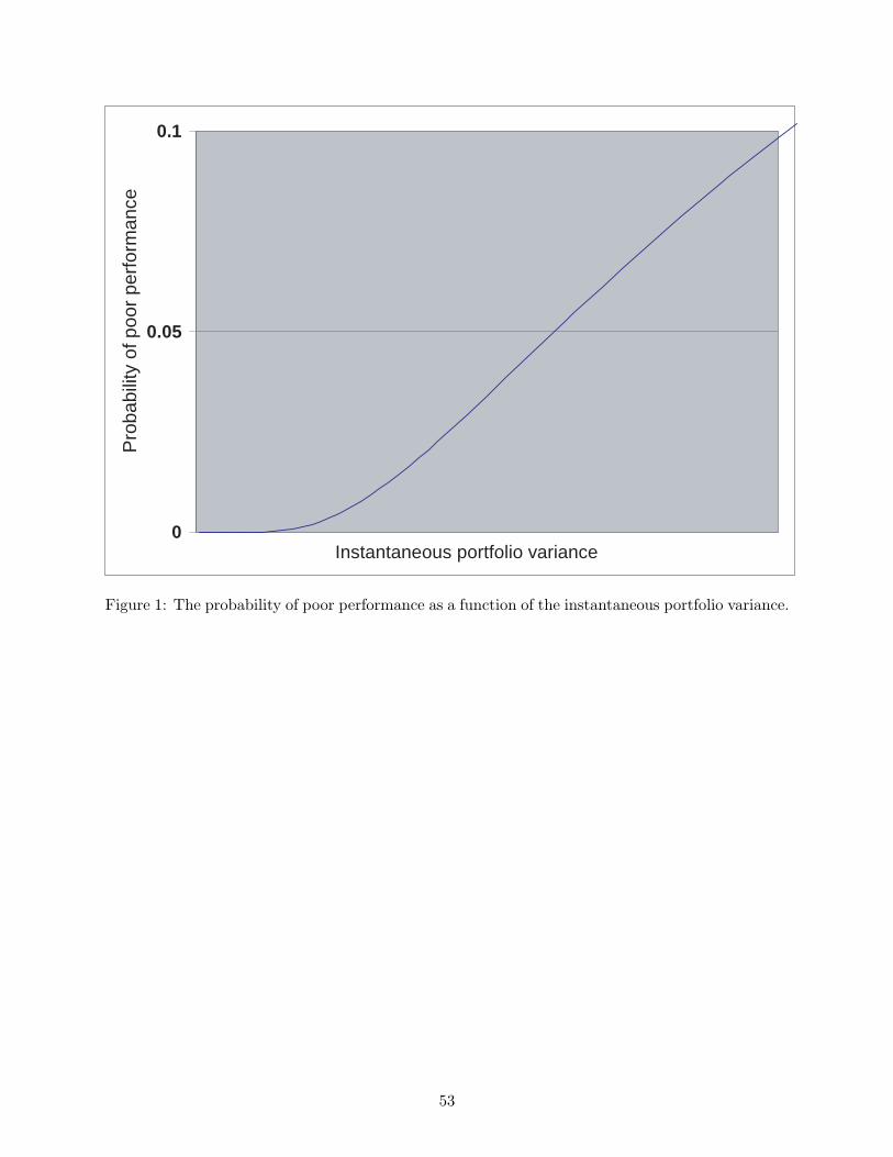
0

0.05

0.1

Instantaneous portfolio variance

Pro

babi

lity

ofpo

orpe

rfor

man

ce

Figure 1: The probability of poor performance as a function of the instantaneous portfolio variance.

53