Fiscal Policy, Sovereign Risk, and Unemployment ∗

Javier Bianchi

Federal Reserve Bank of Minneapolis

and NBER

Pablo Ottonello

University of Michigan

Ignacio Presno

Federal Reserve Board

November 15

Abstract

How should fiscal policy be conducted in the presence of default risk? We address

this question using a sovereign default model with downward wage rigidity. An

increase in government spending during a recession stimulates economic activity

and reduces unemployment. Because the government lacks commitment to

future debt repayments, expansionary fiscal policy increases sovereign spreads

making the fiscal stimulus less desirable. We analyze the optimal fiscal policy

and study quantitatively whether austerity or stimulus is optimal during an

economic slump.

Keywords: sovereign debt, optimal fiscal policy, downward nominal wage rigidity.

JEL Codes: E62, F34, F41, F44, H50.

∗PRELIMINARY AND INCOMPLETE. Latest Draft We would like to thank participants at the2015 Ridge December Forum, Federal Reserve Board and 2016 SED meetings. Disclaimer: The viewsexpressed herein do not necessarily reflect those of the Board of Governors, the Federal Reserve Bank ofMinneapolis or the Federal Reserve System.

1 Introduction

Much of the policy debates on fiscal policy during the Great Recession and the Eurozone

crisis have been centered on whether fiscal stimulus is desirable when there are concerns

about public debt sustainability. There is one view that argues that high unemployment

calls for expansionary government spending (e.g. Krugman, 2015). On the other hand, the

austerity view argues that, with high levels of debt, expansionary government spending

can increase further borrowing costs and the probability of a sovereign default crisis (e.g.

Barro, 2012).

Motivated by this austerity-versus-stimulus debate, we present a model in which debt-

financed government spending can mitigate an economic slump, but the resulting surge

in borrowing increases the vulnerability to a sovereign debt crisis. We study the optimal

fiscal policy and show how the government trades off the stimulus benefits of expanding

government spending with the costs from higher sovereign spreads.

We study optimal fiscal policy in a sovereign default model (Eaton and Gersovitz,

1981; Aguiar and Gopinath, 2006; Arellano, 2008) extended with downward wage rigidity

(Schmitt-Grohe and Uribe, 2016; Na, Schmitt-Grohe, Uribe, and Yue, 2014). We consider

a small open economy with a tradable and a nontradable sector and a fixed exchange

rate regime, or equivalently an economy member of a currency union. Lacking the

ability to depreciate the exchange rate, the economy faces the possibility of involuntary

unemployment. When the economy faces adverse shocks to tradable income, this depresses

aggregate demand and puts downward pressure on the price on non-tradables. Because

the wage is sticky, this reduces labor demand and generates unemployment.

An increase in government spending in non-tradables goods raises the relative price of

non-tradables and stimulates labor demand, thereby reducing unemployment. Because

taxes are distortionary, the government finances the expansion in spending partly by

raising taxes and partly by increasing debt. Confronted with a larger sovereign debt,

investors demand higher spreads on the government bonds to compensate for the risk

of default. Is it then optimal for the government to raise spending, given the increased

burden of sovereign debt and rising borrowing costs? This the key question we address in

our analysis.

Conducting a quantitative study calibrated to the recent Euro Area debt crisis, we

study both the positive and normative implications of fiscal policy. On the positive side,

1

we show that the fiscal multipliers are highly non-linear in the severity of the recession.

We also show that the optimal size of government purchases depends critically on the

sovereign debt level. When the stock of debt is relatively low, government spending

displays a strongly countercyclical role. As debt increases, and the government becomes

more exposed to a sovereign default, the optimal response becomes more austere.

Related Literature. Our paper bridges two strands of the literature. First, our paper

builds on the sovereign debt literature (Eaton and Gersovitz, 1981; Aguiar and Gopinath,

2006; Arellano, 2008). Cuadra, Sanchez, and Sapriza (2010) show that public expenditures

and tax rates are optimally procyclical in a canonical sovereign debt model. Because

spreads are higher in recessions, the government finds it optimal to contract spending and

raise revenues, and do the opposite during expansions. In Arellano and Bai (2014), the

government faces rigidities of fiscal revenues, which can either trigger the need for fiscal

austerity programs, or lead to government default. Our key contribution to this literature

is to consider the role for fiscal policy when there is an aggregate demand channel due to

nominal rigidities.1

Second, our paper also relates to a large literature that studies the role of government

spending as a macroeconomic stabilization tool. Examples in this literature include

Eggertsson (2011), Christiano, Eichenbaum, and Rebelo (2011), Werning (2011) Gali and

Monacelli (2008), Farhi and Werning (2012). This literature shows that when there are

constraints on monetary policy, either because of a zero lower bound or a fixed exchange

rate regime, countercyclical fiscal policy becomes desirable. We contribute to this literature

by introducing the possibility of sovereign default, and studying the implications for optimal

fiscal policy.

Our paper is also related to the empirical literature on fiscal multipliers (for a recent

survey see Ramey (2011)). This literature estimates a wide set of fiscal multipliers. Fiscal

multipliers in our model can be closer to zero or bigger than one, depending on the initial

states.

Roadmap. The paper is organized as follows. Section 2 presents the model and defines

the competitive equilibrium. Section 3 presents the quantitative analysis of the model

1With the exception of Na, Schmitt-Grohe, Uribe, and Yue (2014), this literature abstracts entirely fromnominal rigidities. The focus of Na, Schmitt-Grohe, Uribe, and Yue is on rationalizing why depreciationsof the exchange rate and defaults tend to occur together in the data.

2

calibrated to the Spanish economy. It also evaluates the welfare implications under the

different policy schemes. In section 4 we extend the framework incorporation credit

frictions and study the implications for optimal fiscal policy. Section 5 concludes.

2 Model

This section describes the model economy in which fiscal policy will be studied. We

consider a two-sector small open economy populated by a representative risk-averse

household, a representative firm, and a government. The economy receives a stochastic

endowment of tradable goods and has access to decreasing-returns-to-scale technology

operated by the firm to produce nontradable goods using labor. The household is hand-

to-mouth, consumes tradable and nontradable goods, and inelastically supplies labor in

competitive markets. The labor market is characterized by a downward nominal wage

rigidity, which can give rise to involuntary unemployment (as in Schmitt-Grohe and Uribe

(2016)).

The government is benevolent, and decides external borrowing, taxes, and public

spending on nontradable goods. The government cannot choose monetary policy, assumed

to be determined by a fixed exchange-rate regime. Public spending provides utility to

the household. Due to the presence of nominal wage rigidity and the fixed exchange rate,

public spending can reduce unemployment in the labor markets by affecting relative prices.

The government, however, has only imperfect instruments to finance surges in gN . First,

taxes are assumed to be distortionary. Second, external borrowing consists of one-period

securities, traded with risk-neutral competitive foreign lenders, whose promised repayment

is non-state-contingent. The government does not have commitment to repay and can

default on promised repayment, generating a utility cost to the households and exclusion

from international credit markets.

2.1 Households

Households’ preferences over consumption are described by the intertemporal utility

function:

E0

∞∑t=0

βtu(ct) + v(gNt )− Ω(τt)− ηtψχ,t, (1)

3

where ct denotes private consumption in period t, gNt denotes public spending in nontradable

goods, and τt denotes lump-sum taxes in period t. Let u(.) and g(.) be strictly increasing

and concave functions, and Ω(·) is a strictly increasing and convex function capturing

deadweight losses from taxation. Also, as it will become clear later, ζt is an indicator

function that takes the value of 0 if the government can issue bonds in period t and 1 it is

in financial autarky. The last term in the per-period payoff captures a utility cost from

default, where ψχ,t > 0 depends on the exogenous state of the economy. Finally, β ∈ (0, 1)

is the subjective discount factor, and Et denotes expectation operator conditional on the

information set available at time t.

The consumption good is assumed to be a composite of tradable (cT ) and nontradable

goods (cN), with a constant elasticity of substitution (CES) aggregation technology:

c = C(cT , cN) = [ωc(cT )−µ + (1− ωc)(cN)−µ]−1/µ,

where ωc ∈ (0, 1) and µ > −1. The elasticity of substitution between tradable and

nontradable consumption is therefore 1/(1 + µ).

Our choice of a utility loss from taxes and default, rather than an output cost, is

motivated by the fact that with the former the marginal rate of transformation between

tradable and nontradable goods is not altered when the economy defaults and switches to

autarky.

Each period, households receive a stochastic tradable endowment, yTt , and profits from

the ownership of firms producing nontradable goods, φNt . We assume that yTt is stochastic

and follow a stationary first-order Markov process. Households inelastically supply h

hours of work to the labor markets. Due to the presence of the wage rigidity (discussed in

detail in the next subsections), households will only be able to sell ht ≤ h hours in the

labor markets. The actual hours worked ht is determined by firms and taken as given by

the households. Given that the main focus of the paper is on sovereign debt, we assume

that households are hand-to-mouth and that the government can make proceedings from

external borrowing to the households using lump-sum taxes or transfers, τt, expressed in

tradable units. Households’ sequential budget constraint, expressed in terms of tradables,

is therefore given by

cTt + pNt cNt = yTt + φNt + wtht − τt, (2)

4

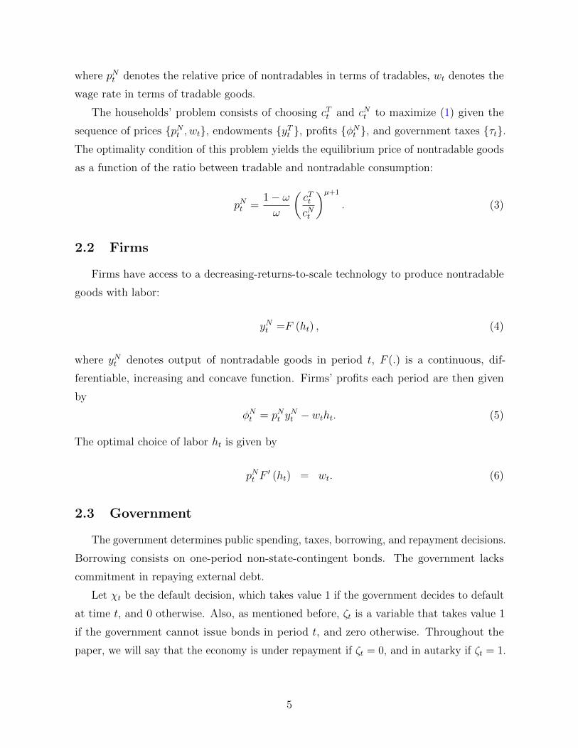
where pNt denotes the relative price of nontradables in terms of tradables, wt denotes the

wage rate in terms of tradable goods.

The households’ problem consists of choosing cTt and cNt to maximize (1) given the

sequence of prices pNt , wt, endowments yTt , profits φNt , and government taxes τt.The optimality condition of this problem yields the equilibrium price of nontradable goods

as a function of the ratio between tradable and nontradable consumption:

pNt =1− ωω

(cTtcNt

)µ+1

. (3)

2.2 Firms

Firms have access to a decreasing-returns-to-scale technology to produce nontradable

goods with labor:

yNt =F (ht) , (4)

where yNt denotes output of nontradable goods in period t, F (.) is a continuous, dif-

ferentiable, increasing and concave function. Firms’ profits each period are then given

by

φNt = pNt yNt − wtht. (5)

The optimal choice of labor ht is given by

pNt F′ (ht) = wt. (6)

2.3 Government

The government determines public spending, taxes, borrowing, and repayment decisions.

Borrowing consists on one-period non-state-contingent bonds. The government lacks

commitment in repaying external debt.

Let χt be the default decision, which takes value 1 if the government decides to default

at time t, and 0 otherwise. Also, as mentioned before, ζt is a variable that takes value 1

if the government cannot issue bonds in period t, and zero otherwise. Throughout the

paper, we will say that the economy is under repayment if ζt = 0, and in autarky if ζt = 1.

5

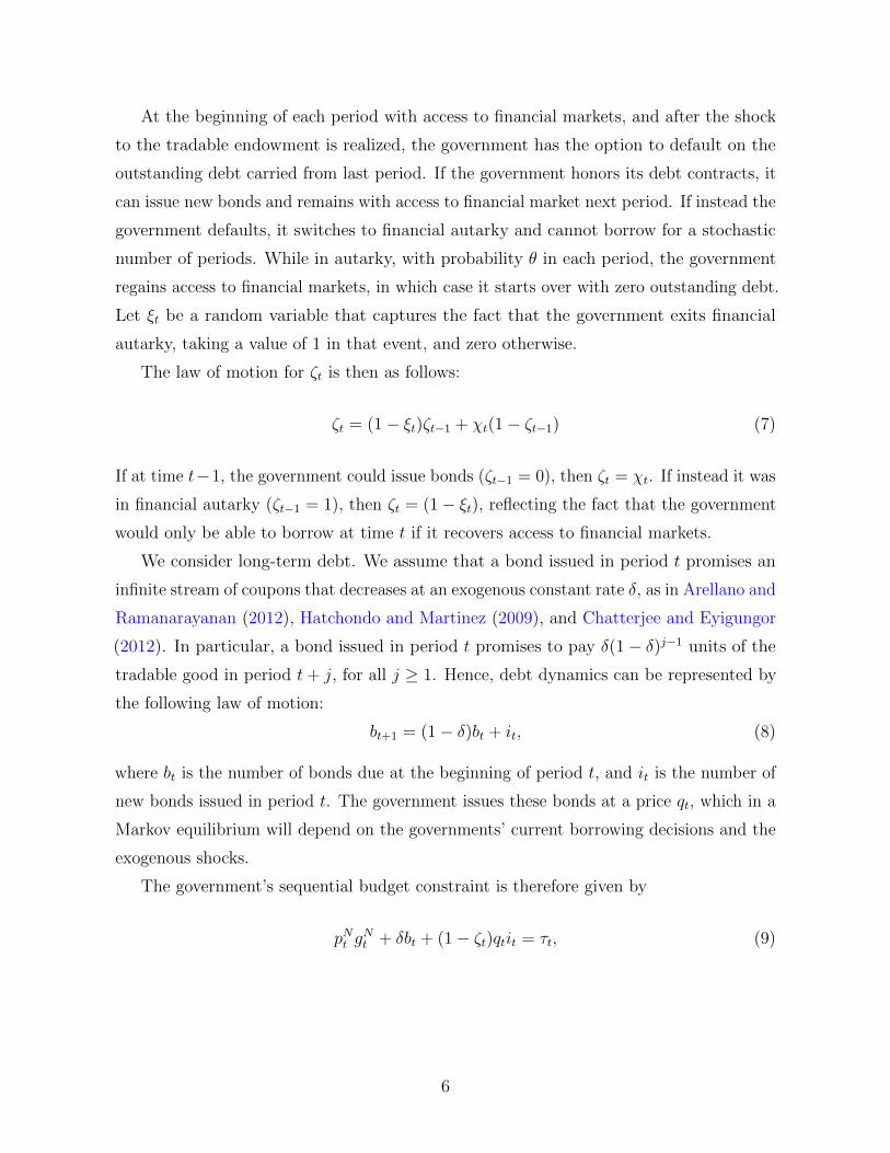
At the beginning of each period with access to financial markets, and after the shock

to the tradable endowment is realized, the government has the option to default on the

outstanding debt carried from last period. If the government honors its debt contracts, it

can issue new bonds and remains with access to financial market next period. If instead the

government defaults, it switches to financial autarky and cannot borrow for a stochastic

number of periods. While in autarky, with probability θ in each period, the government

regains access to financial markets, in which case it starts over with zero outstanding debt.

Let ξt be a random variable that captures the fact that the government exits financial

autarky, taking a value of 1 in that event, and zero otherwise.

The law of motion for ζt is then as follows:

ζt = (1− ξt)ζt−1 + χt(1− ζt−1) (7)

If at time t−1, the government could issue bonds (ζt−1 = 0), then ζt = χt. If instead it was

in financial autarky (ζt−1 = 1), then ζt = (1− ξt), reflecting the fact that the government

would only be able to borrow at time t if it recovers access to financial markets.

We consider long-term debt. We assume that a bond issued in period t promises an

infinite stream of coupons that decreases at an exogenous constant rate δ, as in Arellano and

Ramanarayanan (2012), Hatchondo and Martinez (2009), and Chatterjee and Eyigungor

(2012). In particular, a bond issued in period t promises to pay δ(1− δ)j−1 units of the

tradable good in period t+ j, for all j ≥ 1. Hence, debt dynamics can be represented by

the following law of motion:

bt+1 = (1− δ)bt + it, (8)

where bt is the number of bonds due at the beginning of period t, and it is the number of

new bonds issued in period t. The government issues these bonds at a price qt, which in a

Markov equilibrium will depend on the governments’ current borrowing decisions and the

exogenous shocks.

The government’s sequential budget constraint is therefore given by

pNt gNt + δbt + (1− ζt)qtit = τt, (9)

6

2.4 Foreign Lenders

It is assumed that the sovereign bonds are traded with atomistic, risk-neutral foreign

lenders. In addition to investing through the defaultable bonds, lenders have access to

one-period riskless security paying a gross interest rate R. By an arbitrage condition, bond

prices are then given by:

qt =1

REt((1− δ)qt+1 − χt+1). (10)

Lenders anticipate the government’s default decisions and demand lower bond prices, or

equivalently, higher returns, to compensate for a higher equilibrium probability of default.

2.5 Equilibrium

In equilibrium, the market for nontradable goods clears:

cNt + gNt = F (ht). (11)

Combining the equilibrium price equation (3) with resource constraint (11), the relative

price pt can be expressed as

pNt = P(cTt , ht, gNt ) =

1− ωω

(cTt

F (ht)− gNt

)µ+1

(12)

Combining the households’ budget constraint (2) with the definition of the firms’ profits

and market clearing condition (11), the resource constraint of the economy is given by

cTt = yTt + (1− ζt)[−qtit + δbt] (13)

For the labor markets, it is assumed that nominal wages have a lower bound W , by which

Wt ≥ W for all t. Given that the economy is under a currency peg and assuming that the

law of one price holds for tradable goods and that the price of foreign tradable goods is

constant and normalized to one, the wage rigidity can be expressed as

wt ≥ w, (14)

7

where wt is the real wage and w is the wage lower bound, both in terms of the tradable

good.

Actual hours worked cannot exceed the inelastically supplied level of hours:

ht ≤ h. (15)

Labor market equilibrium implies that the following slackness condition must hold for all

dates and states:

(wt − w)(h− ht

)= 0. (16)

This condition implies that when the nominal wage rigidity binds, the labor market can

exhibit involuntary unemployment, given by h − ht. Similarly, when the nominal wage

rigidity is not binding, the labor market must exhibit full employment.

A competitive equilibrium given government policies in our economy is then defined as

follows:

Definition 1 (Competitive Equilibrium) Given initial debt b0 and ζ0, an exogenous

process yTt , ξt∞t=0, government policies gNt , τt, bt+1, χt∞t=0, a competitive equilibrium is a

sequence of allocations cTt , cNt , ht∞t=0 and prices pNt , wt, qt∞t=0 such that:

1. Allocations solve household’s and firms’ problems at given prices.

2. Government policies satisfy the government budget constraint (9), subject to (7).

3. Bond pricing equation (10) holds.

4. The market for nontradable goods clears.

5. The labor market satisfies (14)-(16).

2.6 Optimal Government Policy

We consider the optimal policy of a benevolent government with no commitment, that

chooses public spending, external borrowing, and taxes to maximize households welfare,

subject to the implementability conditions. We focus on the Markov recursive equilibrium

in which all agents choose sequentially.

Every period the government enters with access to financial markets, it evaluates the

lifetime utility of households if debt contracts are honored against the lifetime utility of

8

households if they are repudiated. Given current (yT , b), the government problem with

access to financial markets can be formulated in recursive form as follows:

V (yT , b) = maxχ∈0,1

(1− χ)V r(yT , b) + χV d(yT ), (P )

where V r(yT , b) and V d(yT ) denote, respectively, the value of repayment, given by the

Bellman equation

V r(yT , b) = maxgN ,τ,b′,h

u(C(cT , F (h)− gN

))+ v(gN)− Ω(τ) + βEV (yT

′, b′) (P r)

subject to

cT + b = yT − q(yT , b′)i

τ = P(cT , h, gN)gN + q(yT , b′)b′ − b,

P(cT , h, gN)F ′ (h) ≥ w,

(P(cT , h, gN)F ′ (h)− w)(h− h) = 0,

and the value of default, given by:

V d(yT ) = maxgN ,τ,h

u(C(yT , F (h)− gN

))+ v(gN)− Ω(τ)− ψχ(yT )

+ βE(1− θ)V d(yT′) + θV (yT

′, 0) (P d)

subject to

τ = P(yT , h, gN)gNt ,

P(yT , h, gN)F ′ (h) ≥ w,

(P(yT , h, gN)F ′ (h)− w)(h− h) = 0.

where q(yT , b′) denote bond price schedule, taken as given by the government.

Let s = (yT , b, ζ) denote the aggregate state of the economy. Let χ(s), cT (s), gN (s), τ(s), b′(s), h(s)be the optimal policy rules associated with the government problem. A Markov perfect

equilibrium is then defined as follows.

9

Definition 2 (Markov perfect equilibrium) A Markov perfect equilibrium is defined

by value functions V (yT , b), V r(yT , b), V d(yT ), policy functions χ(s), cT (s), gN (s), τ(s), b′(s), h(s),and a bond price schedule q(s, b′) such that

1. Given the bond price schedule, policy and functions solve (P ), (P r), and (P d),

2. The bond price schedule satisfies

q(yT , b′) =1

RE(1− χ(yT

′, b′)). (17)

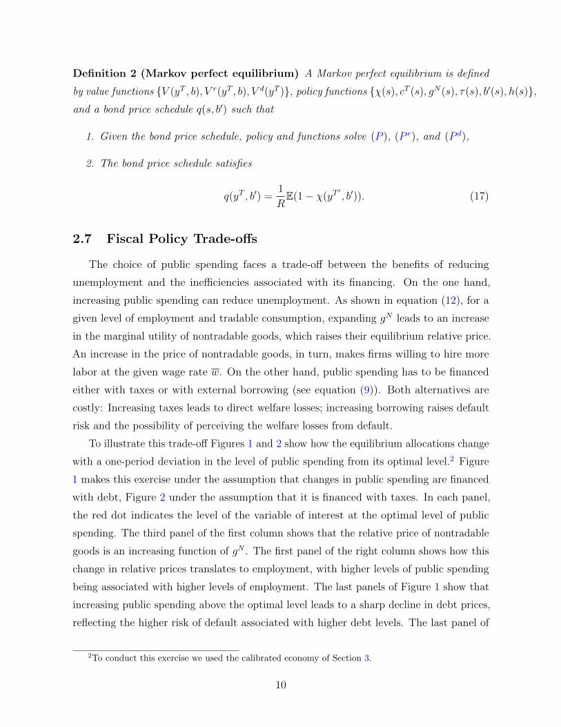
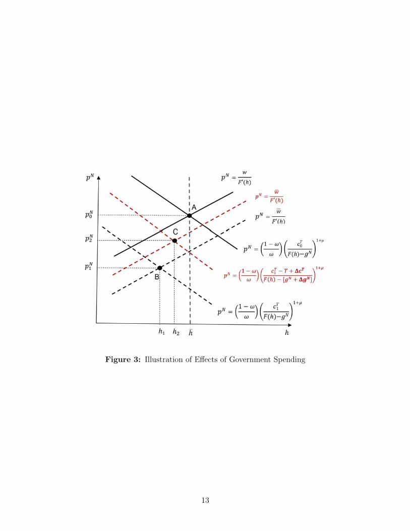
2.7 Fiscal Policy Trade-offs

The choice of public spending faces a trade-off between the benefits of reducing

unemployment and the inefficiencies associated with its financing. On the one hand,

increasing public spending can reduce unemployment. As shown in equation (12), for a

given level of employment and tradable consumption, expanding gN leads to an increase

in the marginal utility of nontradable goods, which raises their equilibrium relative price.

An increase in the price of nontradable goods, in turn, makes firms willing to hire more

labor at the given wage rate w. On the other hand, public spending has to be financed

either with taxes or with external borrowing (see equation (9)). Both alternatives are

costly: Increasing taxes leads to direct welfare losses; increasing borrowing raises default

risk and the possibility of perceiving the welfare losses from default.

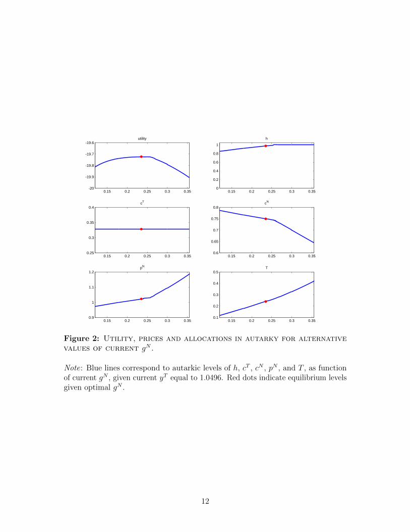
To illustrate this trade-off Figures 1 and 2 show how the equilibrium allocations change

with a one-period deviation in the level of public spending from its optimal level.2 Figure

1 makes this exercise under the assumption that changes in public spending are financed

with debt, Figure 2 under the assumption that it is financed with taxes. In each panel,

the red dot indicates the level of the variable of interest at the optimal level of public

spending. The third panel of the first column shows that the relative price of nontradable

goods is an increasing function of gN . The first panel of the right column shows how this

change in relative prices translates to employment, with higher levels of public spending

being associated with higher levels of employment. The last panels of Figure 1 show that

increasing public spending above the optimal level leads to a sharp decline in debt prices,

reflecting the higher risk of default associated with higher debt levels. The last panel of

2To conduct this exercise we used the calibrated economy of Section 3.

10

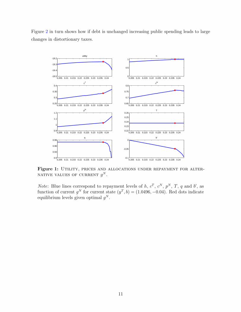
Figure 2 in turn shows how if debt is unchanged increasing public spending leads to large

changes in distortionary taxes.

0.205 0.21 0.215 0.22 0.225 0.23 0.235 0.24-19.5

-19.4

-19.3

-19.2utility

0.205 0.21 0.215 0.22 0.225 0.23 0.235 0.240

0.5

1h

0.205 0.21 0.215 0.22 0.225 0.23 0.235 0.240.25

0.3

0.35

0.4cT

0.205 0.21 0.215 0.22 0.225 0.23 0.235 0.240.65

0.7

0.75

0.8cN

0.205 0.21 0.215 0.22 0.225 0.23 0.235 0.240.9

1

1.1

1.2pN

0.205 0.21 0.215 0.22 0.225 0.23 0.235 0.240.22

0.23

0.24

0.25

0.26T

0.205 0.21 0.215 0.22 0.225 0.23 0.235 0.240.9

0.93

0.96

0.99q

0.205 0.21 0.215 0.22 0.225 0.23 0.235 0.24-0.1

-0.05

0b'

Figure 1: Utility, prices and allocations under repayment for alter-native values of current gN .

Note: Blue lines correspond to repayment levels of h, cT , cN , pN , T , q and b′, asfunction of current gN for current state (yT , b) = (1.0496,−0.04). Red dots indicateequilibrium levels given optimal gN .

11

0.15 0.2 0.25 0.3 0.35-20

-19.9

-19.8

-19.7

-19.6utility

0.15 0.2 0.25 0.3 0.350

0.2

0.4

0.6

0.8

1

h

0.15 0.2 0.25 0.3 0.350.25

0.3

0.35

0.4cT

0.15 0.2 0.25 0.3 0.350.6

0.65

0.7

0.75

0.8cN

0.15 0.2 0.25 0.3 0.350.9

1

1.1

1.2pN

0.15 0.2 0.25 0.3 0.350.1

0.2

0.3

0.4

0.5T

Figure 2: Utility, prices and allocations in autarky for alternativevalues of current gN .

Note: Blue lines correspond to autarkic levels of h, cT , cN , pN , and T , as functionof current gN , given current yT equal to 1.0496. Red dots indicate equilibrium levelsgiven optimal gN .

12

Quick Notes Page 2

Figure 3: Illustration of Effects of Government Spending

13

3 Quantitative Analysis

3.1 Calibration

To characterize the aggregate dynamics under the optimal fiscal policy we calibrate

the model to match key moments in the data at an annual frequency for the Spanish

economy over the period 1995-2015. We consider the following functional forms. We

assume constant relative risk aversion (CRRA) utility functions for private and public

consumption:

u(c) =c1−σ

1− σ,

v(g) =g1−σg

1− σg,

scaled by the relative weights (1−ψg) and ψg, respectively. Also, we consider an isoelastic

form for the production functions in the tradable and nontradable sectors:

F (h) = hα, α ∈ (0, 1). (18)

The maturity of long-term debt will be calibrated to the average duration in the data.

For now, we consider one period debt only.

The specification of the iceberg cost is assumed to be quadratic and symmetric for

taxes and subsidies,

Ω(τ) = ψττ2, (19)

where ψτ > 0 is a parameter that controls for the curvature of function Ω(·) and, hence,

plays a key role in the desirability for tax smoothing in our economy. The more convex

Ω(·) is, the higher the potential benefits are from adopting a smooth path for government

transfers. While the iceberg cost does not affect the implementability conditions in the

government problem, it directly subtracts per-period utility from households.

As mentioned before, in addition to temporary exclusion from financial markets, the

government suffers a direct utility cost of default given by ψχ(yT ). We assume the following

form for this utility loss in autarky:

ψχ(yTt ) = max0, ψ0χ + ψyχ log(yTt ), (20)

14

with α1 > 0. A similar specification but for output costs has been shown by Chatterjee

and Eyigungor (2012) to be crucial for matching bond spreads dynamics, in particular

subduing spreads volatility.

All parameter values used in the baseline calibration are shown in Table 1. The

coefficient of relative risk aversion of private consumption is set to 2, which is standard

in the literature. Similarly, the coefficient of risk aversion of public consumption σg is

also set to 2. The value of the parameter µ implies a Cobb-Douglas specification for the

consumption aggregator and an elasticity of substitution between tradable and nontradable

consumption of 1, slightly above the range of values typically used in other studies. The

share of tradables in the consumption composite implies a ratio of tradable output-to-total

output of 0.25, in line with the data. The relative weight on the public consumption

term in the utility function ψg is calibrated to replicate the average government spending

observed in the data for Spain from 1998 to 2015, which amounts to 18.3 percent of total

output.

The time discount factor β is set to 0.9, within the range of values used in the sovereign

default literature. The utility costs parameters ψ0χ and ψ1

χ chosen to generate a mean and

volatility of bond spreads consistent with the data.

The international risk-free rate R is equal to 1.02, which is roughly the average annual

gross yield on German 5-year government bonds over the period 2000-2015. Data on

bond yields for Germany and Spain has been taken from Deutsche Bank and Banco de

Espana, respectively. The reentry probability θ is set to generate an average autarky

spell of 5 years, which is very close to the average 4.7 years until resumption of financial

access reported by Gelos, Sahay and Sandleris (2011) over the period 1980-2000 for 150

developing countries.

The households’ inelastic supply of hours to work is normalized to 1. The labor share

in the production of nontradable goods is 0.63, which is the estimate found by Uribe (1997)

for Argentina. The lower bound on wages w is set to generate an unemployment rate of

10 percent on average in the simulations, which is lower than the 15 percent observed for

Spain during the period in consideration.

We assume that the tradable endowment yTt follows a log-normal AR(1) process,

log yTt+1 = ρ log yTt + σyεt+1,

15

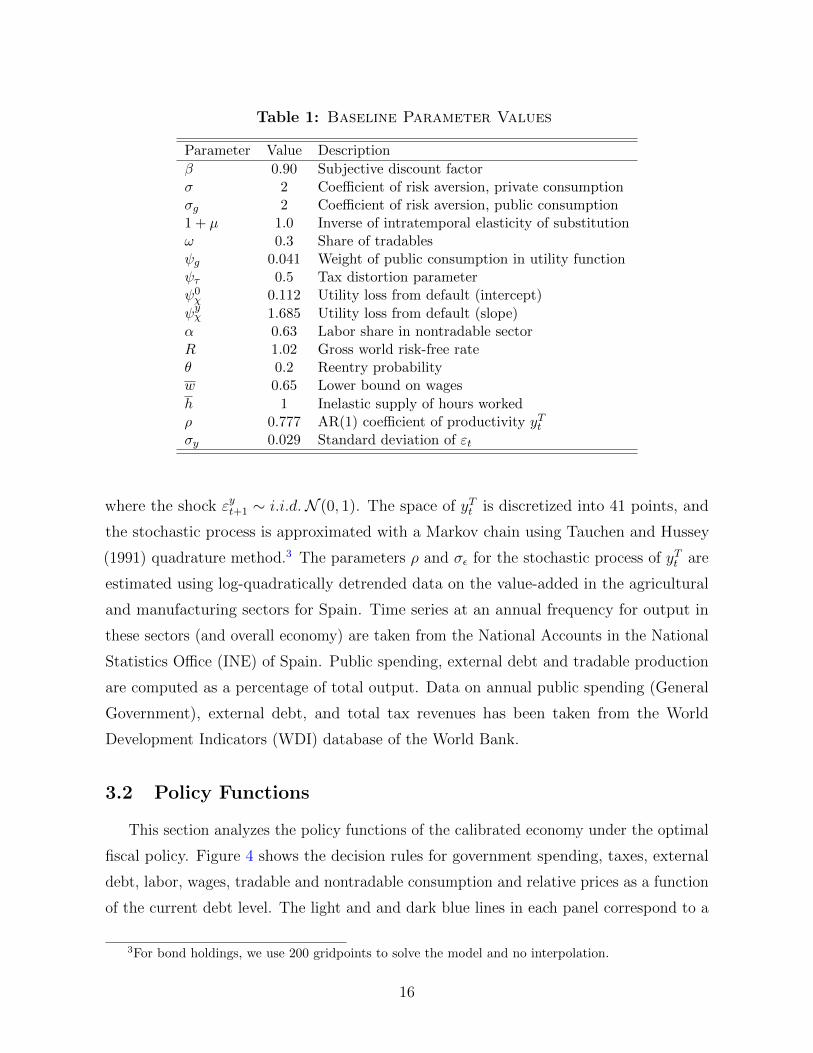
Table 1: Baseline Parameter Values

Parameter Value Description

β 0.90 Subjective discount factorσ 2 Coefficient of risk aversion, private consumptionσg 2 Coefficient of risk aversion, public consumption1 + µ 1.0 Inverse of intratemporal elasticity of substitutionω 0.3 Share of tradablesψg 0.041 Weight of public consumption in utility functionψτ 0.5 Tax distortion parameterψ0χ 0.112 Utility loss from default (intercept)

ψyχ 1.685 Utility loss from default (slope)α 0.63 Labor share in nontradable sectorR 1.02 Gross world risk-free rateθ 0.2 Reentry probabilityw 0.65 Lower bound on wages

h 1 Inelastic supply of hours workedρ 0.777 AR(1) coefficient of productivity yTtσy 0.029 Standard deviation of εt

where the shock εyt+1 ∼ i.i.d.N (0, 1). The space of yTt is discretized into 41 points, and

the stochastic process is approximated with a Markov chain using Tauchen and Hussey

(1991) quadrature method.3 The parameters ρ and σε for the stochastic process of yTt are

estimated using log-quadratically detrended data on the value-added in the agricultural

and manufacturing sectors for Spain. Time series at an annual frequency for output in

these sectors (and overall economy) are taken from the National Accounts in the National

Statistics Office (INE) of Spain. Public spending, external debt and tradable production

are computed as a percentage of total output. Data on annual public spending (General

Government), external debt, and total tax revenues has been taken from the World

Development Indicators (WDI) database of the World Bank.

3.2 Policy Functions

This section analyzes the policy functions of the calibrated economy under the optimal

fiscal policy. Figure 4 shows the decision rules for government spending, taxes, external

debt, labor, wages, tradable and nontradable consumption and relative prices as a function

of the current debt level. The light and and dark blue lines in each panel correspond to a

3For bond holdings, we use 200 gridpoints to solve the model and no interpolation.

16

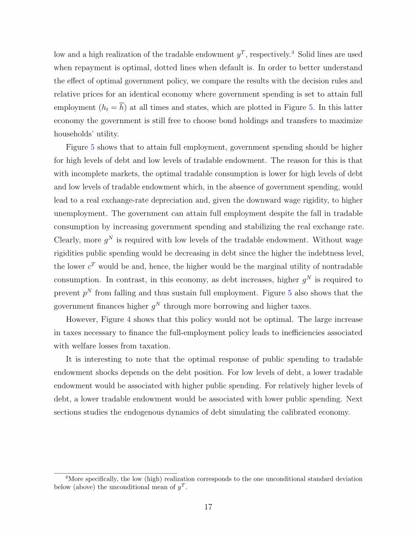
low and a high realization of the tradable endowment yT , respectively.4 Solid lines are used

when repayment is optimal, dotted lines when default is. In order to better understand

the effect of optimal government policy, we compare the results with the decision rules and

relative prices for an identical economy where government spending is set to attain full

employment (ht = h) at all times and states, which are plotted in Figure 5. In this latter

economy the government is still free to choose bond holdings and transfers to maximize

households’ utility.

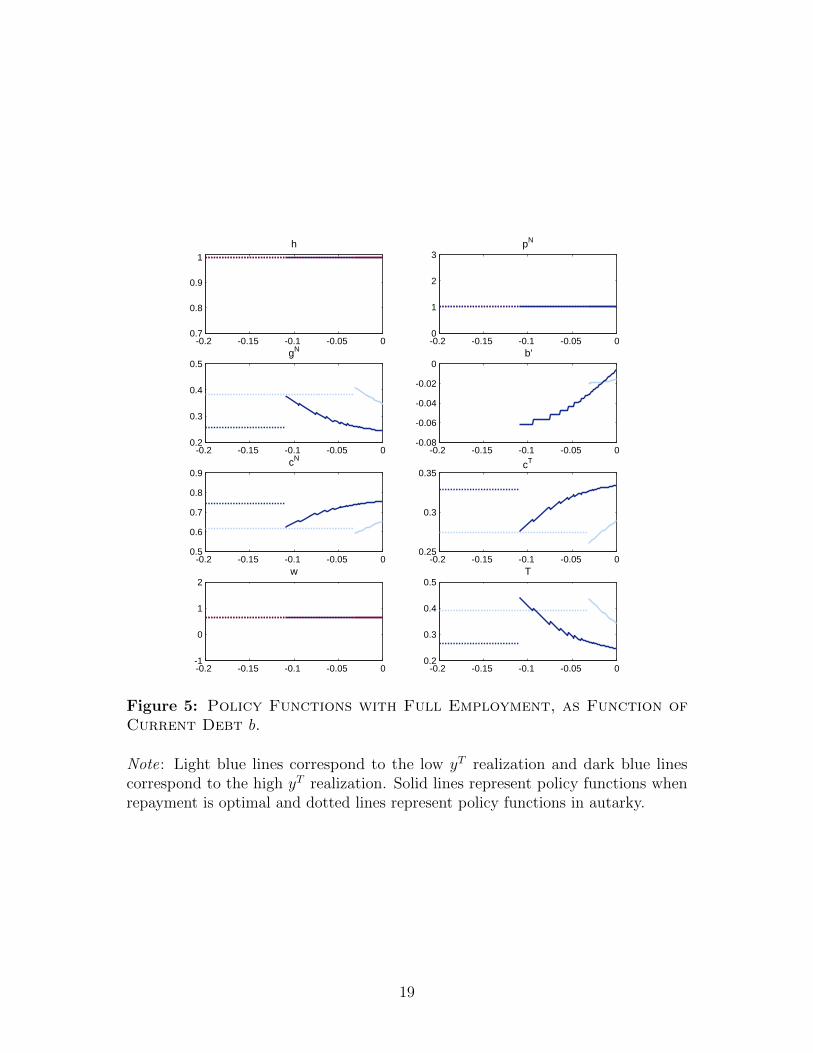
Figure 5 shows that to attain full employment, government spending should be higher

for high levels of debt and low levels of tradable endowment. The reason for this is that

with incomplete markets, the optimal tradable consumption is lower for high levels of debt

and low levels of tradable endowment which, in the absence of government spending, would

lead to a real exchange-rate depreciation and, given the downward wage rigidity, to higher

unemployment. The government can attain full employment despite the fall in tradable

consumption by increasing government spending and stabilizing the real exchange rate.

Clearly, more gN is required with low levels of the tradable endowment. Without wage

rigidities public spending would be decreasing in debt since the higher the indebtness level,

the lower cT would be and, hence, the higher would be the marginal utility of nontradable

consumption. In contrast, in this economy, as debt increases, higher gN is required to

prevent pN from falling and thus sustain full employment. Figure 5 also shows that the

government finances higher gN through more borrowing and higher taxes.

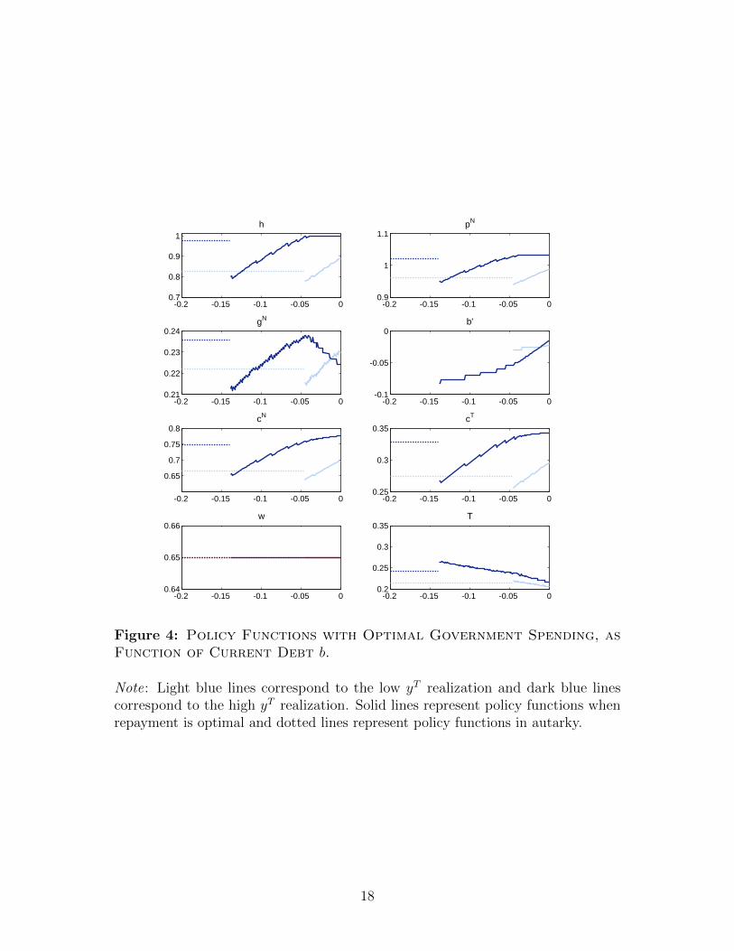
However, Figure 4 shows that this policy would not be optimal. The large increase

in taxes necessary to finance the full-employment policy leads to inefficiencies associated

with welfare losses from taxation.

It is interesting to note that the optimal response of public spending to tradable

endowment shocks depends on the debt position. For low levels of debt, a lower tradable

endowment would be associated with higher public spending. For relatively higher levels of

debt, a lower tradable endowment would be associated with lower public spending. Next

sections studies the endogenous dynamics of debt simulating the calibrated economy.

4More specifically, the low (high) realization corresponds to the one unconditional standard deviationbelow (above) the unconditional mean of yT .

17

-0.2 -0.15 -0.1 -0.05 00.7

0.8

0.9

1h

-0.2 -0.15 -0.1 -0.05 00.9

1

1.1pN

-0.2 -0.15 -0.1 -0.05 00.21

0.22

0.23

0.24gN

-0.2 -0.15 -0.1 -0.05 0-0.1

-0.05

0b'

-0.2 -0.15 -0.1 -0.05 0

0.65

0.7

0.75

0.8cN

-0.2 -0.15 -0.1 -0.05 00.25

0.3

0.35cT

-0.2 -0.15 -0.1 -0.05 00.64

0.65

0.66w

-0.2 -0.15 -0.1 -0.05 00.2

0.25

0.3

0.35T

Figure 4: Policy Functions with Optimal Government Spending, asFunction of Current Debt b.

Note: Light blue lines correspond to the low yT realization and dark blue linescorrespond to the high yT realization. Solid lines represent policy functions whenrepayment is optimal and dotted lines represent policy functions in autarky.

18

-0.2 -0.15 -0.1 -0.05 00.7

0.8

0.9

1h

-0.2 -0.15 -0.1 -0.05 00

1

2

3pN

-0.2 -0.15 -0.1 -0.05 00.2

0.3

0.4

0.5gN

-0.2 -0.15 -0.1 -0.05 0-0.08

-0.06

-0.04

-0.02

0b'

-0.2 -0.15 -0.1 -0.05 00.5

0.6

0.7

0.8

0.9cN

-0.2 -0.15 -0.1 -0.05 00.25

0.3

0.35cT

-0.2 -0.15 -0.1 -0.05 0-1

0

1

2w

-0.2 -0.15 -0.1 -0.05 00.2

0.3

0.4

0.5T

Figure 5: Policy Functions with Full Employment, as Function ofCurrent Debt b.

Note: Light blue lines correspond to the low yT realization and dark blue linescorrespond to the high yT realization. Solid lines represent policy functions whenrepayment is optimal and dotted lines represent policy functions in autarky.

19

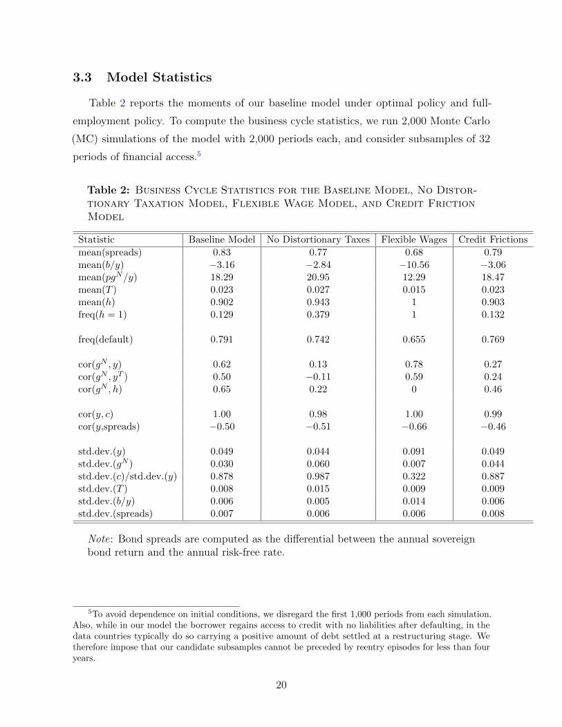
3.3 Model Statistics

Table 2 reports the moments of our baseline model under optimal policy and full-

employment policy. To compute the business cycle statistics, we run 2,000 Monte Carlo

(MC) simulations of the model with 2,000 periods each, and consider subsamples of 32

periods of financial access.5

Table 2: Business Cycle Statistics for the Baseline Model, No Distor-tionary Taxation Model, Flexible Wage Model, and Credit FrictionModel

Statistic Baseline Model No Distortionary Taxes Flexible Wages Credit Frictions

mean(spreads) 0.83 0.77 0.68 0.79mean(b/y) −3.16 −2.84 −10.56 −3.06mean(pgN/y) 18.29 20.95 12.29 18.47mean(T ) 0.023 0.027 0.015 0.023mean(h) 0.902 0.943 1 0.903freq(h = 1) 0.129 0.379 1 0.132

freq(default) 0.791 0.742 0.655 0.769

cor(gN , y) 0.62 0.13 0.78 0.27cor(gN , yT ) 0.50 −0.11 0.59 0.24cor(gN , h) 0.65 0.22 0 0.46

cor(y, c) 1.00 0.98 1.00 0.99cor(y,spreads) −0.50 −0.51 −0.66 −0.46

std.dev.(y) 0.049 0.044 0.091 0.049std.dev.(gN ) 0.030 0.060 0.007 0.044std.dev.(c)/std.dev.(y) 0.878 0.987 0.322 0.887std.dev.(T ) 0.008 0.015 0.009 0.009std.dev.(b/y) 0.006 0.005 0.014 0.006std.dev.(spreads) 0.007 0.006 0.006 0.008

Note: Bond spreads are computed as the differential between the annual sovereignbond return and the annual risk-free rate.

5To avoid dependence on initial conditions, we disregard the first 1,000 periods from each simulation.Also, while in our model the borrower regains access to credit with no liabilities after defaulting, in thedata countries typically do so carrying a positive amount of debt settled at a restructuring stage. Wetherefore impose that our candidate subsamples cannot be preceded by reentry episodes for less than fouryears.

20

The model predicts two key features about the optimal fiscal policy. First, the optimal

fiscal policy is procyclical, with a correlation between public spending and output of 0.62.

This prediction contrast with the −0.30 correlation between public spending and output

observed in the data for the period 1998-2011. Second, public spending is relatively smooth.

The volatility of public spending is 60 percent that of output, which compares to almost

90 percent of private consumption volatility relative to output. In the data government

spending is also found to be relatively smooth with 30 percent of the volatility of output.

To disentangle the mechanisms driving the optimal fiscal policy, Table 2 also reports

the moments of an economy with no distortionary taxes an an economy with flexible wages.

Both ingredients seem to be relevant explaining the patterns of the optimal policy. On

the one hand without distortionary taxation, the optimal policy would be only mildly

procyclical (0.13 correlation of public spending with output) and significantly more volatile

(50 percent more volatile than output). On the other hand, without wage rigidity fiscal

policy would be even more procyclical (0.78 correlation with output) and would practically

not vary over the cycle.

One caveat of this analysis is that the results presented have a debt in the model,

which is much lower than in the data. In future updates, we plan to consider long-term,

which allows for a better fit of the data, as shown by ?.

3.4 Welfare Analysis

In what follows we compare households’ welfare associated with optimal policy against

that resulting from the policy that guarantees full employment in all states, described

in the previous subsection. To do so, we compute the welfare gain of fiscal policy i with

respect to fiscal policy j as the percentage increase rate in current private consumption

under policy j that would make the representative household indifferent between the

two policies. Recall that s = (yT , b, η) denotes the state of the economy.6 Let S be the

associated state space, i.e. S = Y × B × 0, 1. Formally, given the CRRA preference

specification for σ = 2, this compensation denoted by λi,j(s) in current state s is given by

λi,j(s) =∆V (s)

cj(s)−1 −∆V (s)

6Technically, in our model the value of b is only defined if the economy can issue bonds, i.e. η = 0, asdebt plays no role in autarky.

21

with ∆V (s) ≡ V i(s)−V j(s), and where V j and V i correspond to the lifetime utility values

under policies i and j, respectively, and cj(s) is the optimal total consumption decision

rule under policy j.

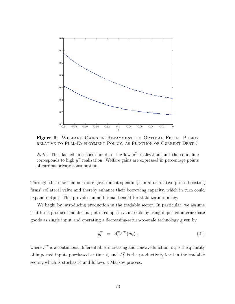
Figure 6 plots the welfare gain of optimal policy under repayment with respect to

the full-employment policy, as a function of the current debt level, for two different yT

levels. The dashed and solid lines correspond to a low and high realizations of the tradable

endowment, respectively.7 Welfare gains vary significantly with the state of the economy

with access to financial markets, taking values that range from around 20 percent to almost

70 percent.8 They are typically more pronounced with low levels of productivity and high

debt, where p tends to be lower. Eliminating involuntary unemployment can be very costly

in terms of welfare, especially in those states, due to its crowding-out effect on private

consumption of nontradables and larger tax distortions associated with higher gN .

Finally, we compute the unconditional welfare gains of optimal government policy

using the ergodic state distributions under the different policy regimes. As before, welfare

gains are expressed in terms of increment of current private consumption. Formally, the

compensation of adopting policy i relative to conducting policy j, denoted by λi,j

satisfies

λi,j

=∆V

(cj)−1 −∆V

with ∆V ≡∑

s∈S µi(s)V i(s)−

∑s∈S µ

j(s)V j(s), and (cj)−1 ≡∑

s∈S µj(s)cj(s), and where

µi and µj are the ergodic distributions of the state s ∈ S under policy i and j, respectively.9

The unconditional compensation rate of optimal policy with respect to the full-employment

regime is 19.96 percent, a non-negligible amount for policy analysis.

4 Firms’ Financial Frictions

In this section, we consider an extension of the baseline model with credit frictions.

We consider a working capital constraint and study the implications for optimal fiscal

policy. As we will see, a financial channel of fiscal policy arises in this extended framework.

7The low (high) endowment level are one unconditional standard deviation below (above) the uncon-ditional mean of yT .

8The welfare gains of optimal policy in autarky for the same yT realizations are 16.28 and 29.14percent, which are not very different from their counterparts when the government can issue bonds.

9For each policy regime, the ergodic distribution of state vector s = (yT , b, η) is computed by collectingthe last observation from each of the 10,000 Monte Carlo simulated paths.

22

-0.2 -0.18 -0.16 -0.14 -0.12 -0.1 -0.08 -0.06 -0.04 -0.02 00.1

0.2

0.3

0.4

0.5

0.6

0.7

0.8

b

Figure 6: Welfare Gains in Repayment of Optimal Fiscal Policyrelative to Full-Employment Policy, as Function of Current Debt b.

Note: The dashed line correspond to the low yT realization and the solid linecorresponds to high yT realization. Welfare gains are expressed in percentage pointsof current private consumption.

Through this new channel more government spending can alter relative prices boosting

firms’ collateral value and thereby enhance their borrowing capacity, which in turn could

expand output. This provides an additional benefit for stabilization policy.

We begin by introducing production in the tradable sector. In particular, we assume

that firms produce tradable output in competitive markets by using imported intermediate

goods as single input and operating a decreasing-return-to-scale technology given by

yTt = ATt FT (mt) , (21)

where F T is a continuous, differentiable, increasing and concave function, mt is the quantity

of imported inputs purchased at time t, and ATt is the productivity level in the tradable

sector, which is stochastic and follows a Markov process.

23

It is assumed that the cost of purchasing imported inputs, pmmt, must be paid in

advance of production. To finance this working capital, firms borrow through within-period

external loans denominated in units of tradables. Due to limited enforcement problems,

firms have to pledge a fraction κt ∈ (0, 1) of gross output as collateral:

pmmt ≤ κt(yTt + pNt y

Nt

). (22)

As in Mendoza (2002) and Bianchi (2012), among others, income can be used as collateral

and thus borrowing is limited to a constant fraction of gross output denominated in

tradable goods. This is also a relevant assumption for emerging economies as it captures

full liability dollarization on the firms’ side. The fraction κt is assumed to be stochastic

and can be interpreted as a financial shock, as in, for example, Jermann and Quadrini

(2012). It is assumed to follow a stationary first-order Markov process.

This collateral constraint (22) will be occasionally restricting the quantity of imported

inputs to firms, depending on the state of the economy.

In each period firms choose mt and ht to maximize profits now given by:

maxmt,ht

ATt FT (mt) + pNt F

N(ht)− pmmt − wtht

subject to the technology constraints (21) and (4) and the collateral constraint (22), given

prices pNt and wages wt.

Let λt denote the Lagrange multiplier associated with the collateral constraint (22).

The first-order conditions with respect to mt and ht are

ATt FTm(mt)(1 + κtλt) = pm(1 + λt)

pNt FNh (ht)(1 + κtλt) = wt

where F Tm(m) ≡ ∂FT (m)

∂mand FN

h (h) ≡ ∂FN (h)∂h

. Due to the collateral constraint, the FOCs

are altered relative to the frictionless economy. As long as the collateral constraint binds,

λt > 0, and hence the marginal product of each input does not equal its respective marginal

cost.

24

Furthermore, the complementary slackness conditions are

λt ≥ 0, λt(κt(yTt + pNt y

Nt

)− pmmt

)= 0. (23)

We assume that the financial shock κt can take only two values: κL and κH , with

0 < κL < κH . In particular, we set κL = 0.08 to generate an average drop of total

value-added of 10 percent on impact, which is roughly the fall observed in output during

sudden stop episodes. And the value for κH is chosen sufficiently high that the collateral

constraint does not bind for any state in equilibrium.

Also, we consider the following transition probability matrix for κt: Π(κH |κH) = 0.9

and Π(κH |κL) = 1. The latter probability is set to match the mean duration of a sudden

stop of around one year, as observed in the data from 1970 to 2011. The former probability

is then chosen to generate a 9-percent annual probability of occurrence of a sudden stop

in the asymptotic distribution, which is in the range of the data.

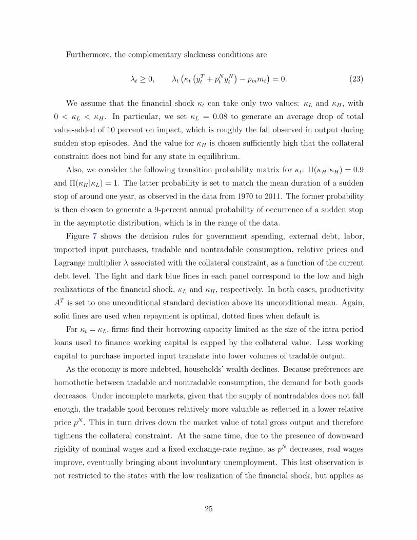
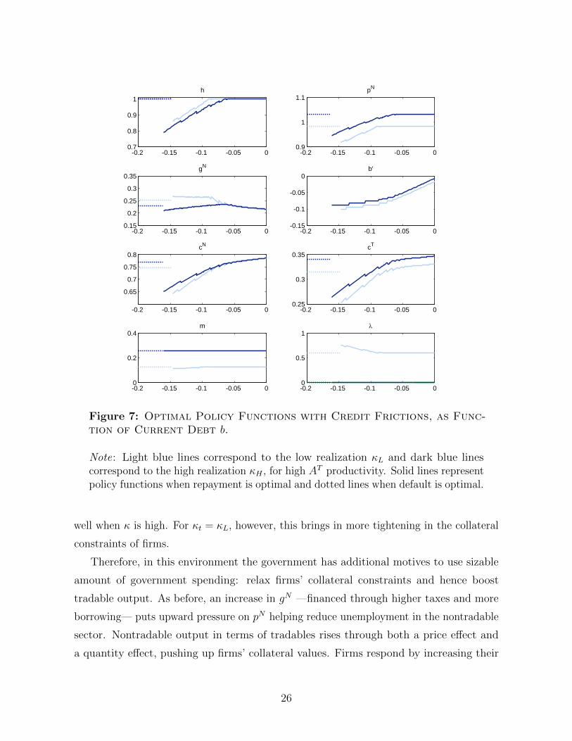
Figure 7 shows the decision rules for government spending, external debt, labor,

imported input purchases, tradable and nontradable consumption, relative prices and

Lagrange multiplier λ associated with the collateral constraint, as a function of the current

debt level. The light and dark blue lines in each panel correspond to the low and high

realizations of the financial shock, κL and κH , respectively. In both cases, productivity

AT is set to one unconditional standard deviation above its unconditional mean. Again,

solid lines are used when repayment is optimal, dotted lines when default is.

For κt = κL, firms find their borrowing capacity limited as the size of the intra-period

loans used to finance working capital is capped by the collateral value. Less working

capital to purchase imported input translate into lower volumes of tradable output.

As the economy is more indebted, households’ wealth declines. Because preferences are

homothetic between tradable and nontradable consumption, the demand for both goods

decreases. Under incomplete markets, given that the supply of nontradables does not fall

enough, the tradable good becomes relatively more valuable as reflected in a lower relative

price pN . This in turn drives down the market value of total gross output and therefore

tightens the collateral constraint. At the same time, due to the presence of downward

rigidity of nominal wages and a fixed exchange-rate regime, as pN decreases, real wages

improve, eventually bringing about involuntary unemployment. This last observation is

not restricted to the states with the low realization of the financial shock, but applies as

25

-0.2 -0.15 -0.1 -0.05 00.7

0.8

0.9

1h

-0.2 -0.15 -0.1 -0.05 00.9

1

1.1pN

-0.2 -0.15 -0.1 -0.05 00.15

0.2

0.25

0.3

0.35gN

-0.2 -0.15 -0.1 -0.05 0-0.15

-0.1

-0.05

0b'

-0.2 -0.15 -0.1 -0.05 0

0.65

0.7

0.75

0.8cN

-0.2 -0.15 -0.1 -0.05 00.25

0.3

0.35cT

-0.2 -0.15 -0.1 -0.05 00

0.2

0.4m

-0.2 -0.15 -0.1 -0.05 00

0.5

1

Figure 7: Optimal Policy Functions with Credit Frictions, as Func-tion of Current Debt b.

Note: Light blue lines correspond to the low realization κL and dark blue linescorrespond to the high realization κH , for high AT productivity. Solid lines representpolicy functions when repayment is optimal and dotted lines when default is optimal.

well when κ is high. For κt = κL, however, this brings in more tightening in the collateral

constraints of firms.

Therefore, in this environment the government has additional motives to use sizable

amount of government spending: relax firms’ collateral constraints and hence boost

tradable output. As before, an increase in gN —financed through higher taxes and more

borrowing— puts upward pressure on pN helping reduce unemployment in the nontradable

sector. Nontradable output in terms of tradables rises through both a price effect and

a quantity effect, pushing up firms’ collateral values. Firms respond by increasing their

26

demand of imported inputs and thereby tradable output expands. Interestingly, as shown

in the figure, the government optimally chooses to sustain relatively higher employment

with κL by allocating substantially more resources to government spending. By doing

so, it partly mitigates the worsening of firms’ credit conditions preventing the Lagrange

multiplier λ associated with the collateral constraint from rising even further. As current

debt continues increasing, it eventually becomes too costly for fiscal policy to avoid a

credit tightening for firms and hence we observe λ drifting up. Not surprisingly, as shown

in Table 2, fiscal policy becomes more volatile than in the baseline model. Also, optimal

gN is less procyclical.

The reduction in nontradable consumption —due to the crowding out of government

spending— is more than compensated by a rise in government spending and in tradable

consumption —following the relaxation of collateral constraints— leading to higher welfare

for households.

5 Conclusion

We studied the positive and normative implications of fiscal policy in a sovereign

default model extended with downward nominal rigidity. The presence of downward wage

rigidity creates a role for stabilization policy during recession. Sovereign default risk,

however, makes it costly to run debt financed stimulus.

We show that the stabilization effects of fiscal policy are highly non-linear in the

severity of the recession. When the level of unemployment is high, fiscal multipliers are

large, and can exceed unity when spending is debt financed. On the normative side, the

optimal amount of government spending depends critically on the sovereign debt level.

When the stock of debt is relatively low, recessions calls for strong stabilization policy.

As debt increases and the government becomes more exposed to a sovereign default, the

optimal response becomes more austere.

In work in progress we are considering how long-term debt maturity allows for a more

active stabilization policy. Moreover, we are also considering aspects of commitment in

the conduct of optimal fiscal policy and in the design of fiscal rules.

27

References

Aguiar, M., and G. Gopinath (2006): “Defaultable Debt, Interest Rates and the

Current Account,” Journal of International Economics, 69(1), 64–83.

Arellano, C. (2008): “Default Risk and Income Fluctuations in Emerging Economies,”

American Economic Review, 98(3), 690–712.

Arellano, C., and Y. Bai (2014): “Fiscal Austerity during Debt Crises,” Discussion

paper, Working paper, University of Rochester.

Arellano, C., and A. Ramanarayanan (2012): “Default and the Maturity Structure

in Sovereign Bonds,” Journal of Political Economy, 120(2), 187–232.

Barro, R. (2012): “Stimulus Spending Keeps Failing,” The Wall Street Journal May

9. http://www.wsj.com/articles/SB10001424052702304451104577390482019129156?mg=id-

wsj.

Chatterjee, S., and B. Eyigungor (2012): “Maturity, Indebtedness, and Default

Risk,” American Economic Review, 102(6), 2674–2699.

Christiano, L., M. Eichenbaum, and S. Rebelo (2011): “When is the government

spending multiplier large?,” Journal of Political Economy.

Cuadra, G., J. M. Sanchez, and H. Sapriza (2010): “Fiscal policy and default risk

in emerging markets,” Review of Economic Dynamics, 13(2), 452–469.

Eaton, J., and M. Gersovitz (1981): “Debt with Potential Repudiation: Theoretical

and Empirical Analysis,” Review of Economic Studies, 48(2), 289–309.

Eggertsson, G. B. (2011): “What fiscal policy is effective at zero interest rates?,” in

NBER Macroeconomics Annual 2010, Volume 25, pp. 59–112. University of Chicago Press.

Farhi, E., and I. Werning (2012): “Fiscal multipliers: Liquidity traps and currency

unions,” Discussion paper, National Bureau of Economic Research.

Gali, J., and T. Monacelli (2008): “Optimal monetary and fiscal policy in a currency

union,” Journal of international economics, 76(1), 116–132.

Hatchondo, J. C., and L. Martinez (2009): “Long-Duration Bonds and Sovereign

Defaults,” Journal of International Economics, 79(1), 117–125.

Krugman, P. (2015): “Austerity Arithmetic,” The New York Times

http://krugman.blogs.nytimes.com/2015/07/05/austerity-arithmetic/.

Na, S., S. Schmitt-Grohe, M. Uribe, and V. Z. Yue (2014): “A Model of the Twin

Ds: Optimal Default and Devaluation,” .

Ramey, V. A. (2011): “Can government purchases stimulate the economy?,” Journal of

Economic Literature, 49(3), 673–685.

Schmitt-Grohe, S., and M. Uribe (2016): “Downward nominal wage rigidity, currency

pegs, and involuntary unemployment,” Journal of Political Economy, 2.

28

Uribe, M. (1997): “Exchange-rate-based inflation stabilization: the initial real effects of

credible plans,” Journal of monetary Economics, 39(2), 197–221.

Werning, I. (2011): “Managing a liquidity trap: Monetary and fiscal policy,” Discussion

paper, National Bureau of Economic Research.

29