Downward Nominal Wage Rigidity, Currency Pegs, and ...mu2166/dnwr_pegs_iu/paper.pdf · Downward...

Downward Nominal Wage Rigidity, CurrencyPegs, and Involuntary Unemployment

Stephanie Schmitt-Grohe

Columbia University, Centre for Economic Policy Research, and National Bureau of Economic Research

Martın Uribe

Columbia University and National Bureau of Economic Research

This paper analyzes the inefficiencies arising from the combinationof fixed exchange rates, nominal rigidity, and free capital mobility. Wedocument that nominal wages are downwardly rigid in emerging coun-tries. We develop an open-economy model that incorporates this fric-tion. The model predicts that the combination of a currency peg andfree capital mobility creates a negative externality that causes overbor-rowing during booms and high unemployment during contractions.Optimal capital controls are shown to be prudential. For plausible cali-brations, they reduce unemployment by around 5 percentage points.The optimal exchange rate policy eliminates unemployment and callsfor large devaluations during crises.

I. Introduction

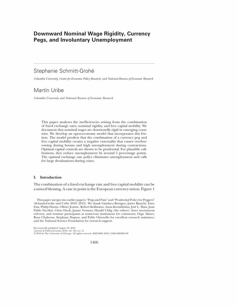
The combination of a fixed exchange rate and free capital mobility can beamixed blessing. A case in point is the European currency union. Figure 1

This papermerges two earlier papers: “Pegs and Pain” and “Prudential Policy for Peggers”(Schmitt-Grohé and Uribe 2010, 2012). We thank Gianluca Benigno, Javier Bianchi, EsterFaia, Philip Harms, Olivier Jeanne, Robert Kollmann, Anna Kormilitsina, José L. Maia, JuanPablo Nicolini, Chris Otrok, Jaume Ventura, Harald Uhlig (the editor), three anonymousreferees, and seminar participants at numerous institutions for comments; Ozge Akinci,Ryan Chahrour, Stephane Dupraz, and Pablo Ottonello for excellent research assistance;and the National Science Foundation for research support.

Electronically published August 30, 2016[ Journal of Political Economy, 2016, vol. 124, no. 5]© 2016 by The University of Chicago. All rights reserved. 0022-3808/2016/12405-0003$10.00

1466

FIG.1.—

Boom-bustcyclein

peripheralEurope:20

00–20

11.D

ataSo

urce:Eurostat.S

ample

period,2

000:Q4–

2011

:Q3.

Datarepresentarithmeticmean

ofBulgaria,Cyprus,Estonia,Greece,

Irelan

d,Lithuan

ia,Latvia,

Portugal,Sp

ain,Slovenia,an

dSlovakia.

Thevertical

dotted

lineindicates

2008

:Q2,

the

onsetoftheGreat

Contractionin

Europe.

Detaileddatasources

andco

untry-by-co

untryplotsareavailable

inonlineap

pen

dix

A.T

hedataareprovided

withtheonlinematerialsofthispap

er.Colorversionavailable

asan

onlineen

han

cemen

t.

displays the average current-account-to-GDP ratio, an index of nominalhourly wages in euros, and the rate of unemployment for a group of pe-ripheral European countries that were either on or pegging to the euroover theperiod 2000–2011. In the early 2000s, these countries enjoyed largecapital inflows, which, through their expansionary effect on domestic ab-sorption, led to sizable appreciations in hourly wages. With the onset ofthe global recession in 2008, capital inflows dried up and aggregate de-mand collapsed. At the same time, nominal wages remained at the levelthey had achieved at the peak of the boom.The combination of depressedlevels of aggregate demand and high nominal wages was associated with amassive increase in involuntary unemployment. In turn, local monetaryauthorities were unable to reduce real wages via a devaluation becauseof their commitment to the currency union.This narrative evokes several interrelated questions. What is the opti-

mal exchange rate policy in an open economy with downward nominalwage rigidity? What are the welfare costs of currency pegs vis-à-vis the op-timal exchange rate policy in the presence of downward nominal wagerigidity? Can fixed exchange rate regimes benefit from imposing capitalcontrols? If so, are optimal capital controls prudential in nature; that is,is it optimal to tax capital inflows during booms and subsidize them dur-ing contractions? How large are the welfare gains of optimal capital con-trols for peggers?In this paper, we address these five questions both analytically and

quantitatively. To this end, we develop a model of an open economy withdownward nominal wage rigidity. The motivation for focusing on down-ward nominal wage rigidity is empirical. There exists a large literature sug-gesting that downward nominal wage rigidity is pervasive in developedcountries. In this paper, we provide new evidence suggesting that this isalso the case among emerging-market economies.The model predicts an endogenous connection between macroeco-

nomic volatility and the mean level of unemployment. This connectionis due to the nature of the assumed labor contract, according to which em-ployment is demand determined during contractions but supply and de-mand determined during booms. As a result, involuntary unemploymentemerges during downturns and full employment during booms. Conse-quently, aggregate fluctuations cause unemployment on average. Impor-tantly, the average level of unemployment is increasing in the amplitudeof the business cycle, opening the door to large welfare gains frommacro-economic stabilization policy.The paper establishes that the combination of downward nominal wage

rigidity, a fixed exchange rate, and free capital mobility creates a nega-tive externality. The externality causes overborrowing during booms andexcessive unemployment during contractions. The nature of the external-

1468 journal of political economy

ity is that expansions in aggregate demand drive up wages, putting theeconomy in a vulnerable situation. For in the contractionary phase ofthe cycle, downward nominal wage rigidity and a fixed exchange rate pre-vent real wages from falling to the level consistent with full employment.Agents understand thismechanism but are too small to internalize the factthat their individual expenditure decisions collectively cause inefficientlylarge increases in wages during expansions.The existence of the externality creates a rationale for government in-

tervention. We consider two types of policy intervention. First, we studyinterventions that achieve the first-best allocation. We show that the first-best allocation can be brought about either via exchange rate policy orvia labor or production subsidies at the level of the firm financed by in-come taxes levied at the level of the household.The optimal exchange rate policy consists in engineering large devalu-

ations of the domestic currency during contractions. The purpose of thesedevaluations is to reduce the real value of wages. Importantly, these opti-mal devaluations are not of the beggar-thy-neighbor type because theydo not aim to foster exports by altering the terms of trade. Rather, theyare geared toward correcting the distortion in the labor market createdby downward nominal wage rigidity. Versions of the model calibrated toemerging-country data predict that boom-bust episodes like the ones thattook place in Argentina in 2001 or in peripheral Europe in 2008, in whichoutput falls by two standard deviations from peak to trough over a timespan of 10 quarters, call for devaluations of about 100 percent.The second type of policy intervention we consider is one in which the

policy maker is constrained to stick to a currency peg and faces limita-tions to change domestic fiscal policy. Instead, he resorts to imposing cap-ital controls. We show that in fixed exchange rate economies the Ramsey-optimal capital control tax is prudential in nature, as it restricts capitalinflows in good times and subsidizes external borrowing in bad times.The benevolent government has an incentive to levy taxes on externaldebt during expansions as a way to limit nominal wage growth. Moder-ating wage growth during booms helps ameliorate the unemploymentproblem caused by downward wage rigidity during subsequent contrac-tions. We show that the government determines the optimal capital con-trol policy as the solution to a trade-off between intertemporal distortionscaused by the capital controls themselves and static distortions causedby the combination of downward nominal wage rigidity and a fixed ex-change rate.Quantitative analysis based on a plausible calibration of the model to

emerging-country data suggests that currency pegs coupled with free cap-ital mobility lead to high average levels of unemployment of more than8 percent. In turn, large levels of unemployment translate into large wel-

downward nominal wage rigidity 1469

fare losses. Capital controls are shown to be highly effective at curbingoverborrowing during booms and reducing unemployment during busts.In the baseline calibration, optimal capital controls reduce the averagerate of unemployment fromover 8 percent to below 3 percent. Thismeansthat the trade-off faced by the policy maker between alleviating the staticdistortions in the labor markets and interfering with the efficient inter-temporal allocation of tradable absorption through capital controls is re-solved largely in favor of the former.This paper is related to the Mundellian literature on the trilemma of

international finance, according to which a country cannot have at thesame time a fixed exchange rate, free capital mobility, and an indepen-dent interest rate policy. A number of studies have analyzed the welfareconsequences of currency pegs in the context of models with nominalrigidities (e.g., Kollmann 2002; Galí and Monacelli 2005). There is alsoa body of work on the role of capital controls as a stabilization instrument.A strand of this literature stresses financial distortions, such as collateralconstraints on external borrowing as a rationale for capital controls (Au-ernheimer and García-Saltos 2000; Uribe 2006, 2007; Lorenzoni 2008;Caballero and Lorenzoni 2009; Korinek 2010; Benigno et al. 2011; Bianchi2011; Bianchi and Mendoza 2012; Jeanne and Korinek 2013). Anotherline of work is based on the classical trade theoretic argument that gov-ernments of large countries have incentives to apply capital controls asa means to induce households to internalize the country’s market powerin financialmarkets (e.g., Obstfeld andRogoff 1996; Costinot, Lorenzoni,and Werning 2011). Our theory of capital controls is distinct from theabove two in that it does not assume the existence of collateral constraintsor market power in financial markets. In a recent related paper, Farhiand Werning (2012) study capital controls in the context of a perfect-foresight, linearized version of the Galí and Monacelli (2005) sticky-pricemodel.The remainder of the paper is organized as follows. Section II develops

the theoretical model. Section III identifies the negative externality aris-ing from the combination of downward nominal wage rigidity, fixed ex-change rates, and free capital mobility. Sections IV, V, andVI characterizeequilibrium dynamics under optimal exchange rate policy, optimal fiscalpolicy under a currency peg, and optimal capital control policy under acurrency peg, respectively. Section VII shows bymeans of an analytical ex-ample thatoptimal capital controls areprudential. SectionVIIIpresentsem-pirical evidence on downward nominal wage rigidity in emerging coun-tries. Section IX analyzes quantitatively the adjustment of the economy toa boom-bust cycle under the various policy arrangements described above.It also contains themain quantitative results on the effects of the aforemen-tioned policy interventions on overborrowing, average unemployment,and welfare. Section X presents conclusions.


II. An Open Economy with Downward Nominal Wage Rigidity

We develop a model of a small open economy in which nominal wagesare downwardly rigid. The model features two types of goods, tradablesand nontradables. The economy is driven by two exogenous shocks, acountry–interest rate shock and a terms-of-trade shock.

A. Households

The economy is populated by a large number of identical householdswith preferences described by the utility function

E0o∞

t50

btU ðctÞ, (1)

where ct denotes consumption, U is a strictly increasing and concave pe-riod utility function, and b ∈ (0, 1) is the subjective discount factor. Thesymbol Et denotes the mathematical expectations operator conditionalon information available in period t. The consumption good is a com-posite of tradable consumption, cTt , and nontradable consumption, cNt .The aggregation technology has the form

ct 5 AðcTt , cNt Þ, (2)

whereA(�, �) is an increasing, concave, and linearly homogeneous function.We assume full liability dollarization. Specifically, households have ac-

cess to a one-period, internationally traded, state-noncontingent bondde-nominated in tradables. We let dt denote the level of debt assumed in pe-riod t2 1 and due in period t and rt the interest rate on debt held betweenperiods t and t1 1. The sequential budget constraint of the household isgiven by

PTt c

Tt 1 PN

t cNt 1 Etdt 5 PT

t yTt 1 Wtht 1 Ft 1

Etdt11

1 1 rt, (3)

where PTt denotes the nominal price of tradable goods, PN

t the nominalprice of nontradable goods, Et the nominal exchange rate defined as thedomestic currency price of one unit of foreign currency, yTt the endow-ment of traded goods, Wt the nominal wage rate, ht hours worked, andFt nominal profits from the ownership of firms. The variables rt and yTtare assumed to be exogenous and stochastic. Movements in yTt can be in-terpreted either as shocks to the physical availability of tradable goods oras shocks to the country’s terms of trade.Households supply inelastically �h hours to the labor market each pe-

riod. The assumption of an inelastic labor supply is motivated in part bymicroeconometric evidence (e.g., Blundell andMaCurdy 1999) andmac-


roeconometric evidence from models with nominal rigidities (e.g., SmetsandWouters 2007; Justiniano, Primiceri, and Tambalotti 2010) suggestingthat the labor supply elasticity is near zero. A second reason for assumingan inelastic labor supply is that it makes the workings of our two-sectormodel more transparent. In section G.5 of the online appendix, we relaxthis assumption by endogenizing the labor supply decision. Because of thepresence of downward nominal wage rigidity, householdsmay not be ableto sell all of the hours they supply. As a result, households take employ-ment, ht ≤ �h, as exogenously given.Households are assumed to be subject to the following debt limit, which

prevents them from engaging in Ponzi schemes:

dt11 ≤ �d, (4)

where �d denotes the natural debt limit.We assume that the law of one price holds for tradables. Specifically, let-

tingPT*t denote the foreign currency priceof tradables, the lawof oneprice

implies that PTt 5 P

T*t Et : We further assume that the foreign currency

price of tradables is constant and normalized to unity, PT*t 5 1. In the

quantitative analysis, we relax this assumption. Thus, we have that thenominal price of tradables equals the nominal exchange rate, PT

t 5 Et :Households choose contingent plans fct , cTt , cNt , dt11g to maximize (1)

subject to (2)–(4) taking as given PTt , P

Nt , Et, Wt, ht, Ft, rt, and yTt . Letting

pt ;PNt

PTt

denote the relative price of nontradables in terms of tradables and usingthe fact that PT

t 5 Et , the optimality conditions associated with this prob-lem are (2)–(4) and

A2ðcTt , cNt ÞA1ðcTt , cNt Þ

5 pt , (5)

lt 5 U 0ðctÞA1ðcTt , cNt Þ,

lt

1 1 rt5 bEtlt11 1 mt ,

mt ≥ 0,

mtðdt11 2 �d Þ 5 0,

(6)

where lt=PTt and mt denote the Lagrange multipliers associated with (3)

and (4), respectively.


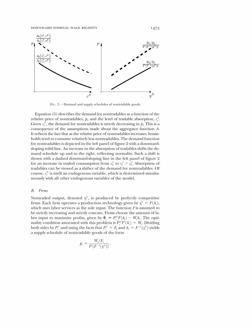
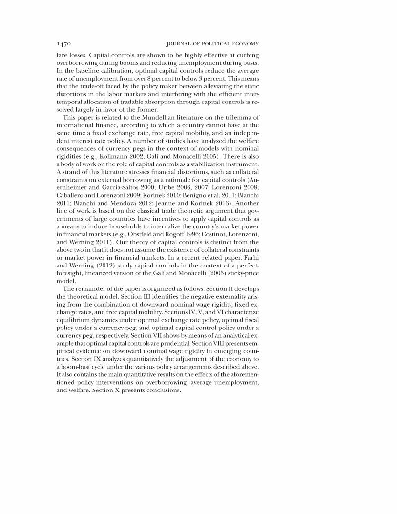
Equation (5) describes the demand for nontradables as a function of therelative price of nontradables, pt, and the level of tradable absorption, cTt .Given cTt , the demand for nontradables is strictly decreasing in pt. This is aconsequence of the assumptions made about the aggregator function A.It reflects the fact that as the relative price of nontradables increases, house-holds tend to consume relatively less nontradables. The demand functionfor nontradables is depicted in the left panel of figure 2 with a downward-sloping solid line. An increase in the absorption of tradables shifts the de-mand schedule up and to the right, reflecting normality. Such a shift isshown with a dashed downward-sloping line in the left panel of figure 2for an increase in traded consumption from cT0 to cT1 > cT0 . Absorption oftradables can be viewed as a shifter of the demand for nontradables. Ofcourse, cTt is itself an endogenous variable, which is determined simulta-neously with all other endogenous variables of the model.

B. Firms

Nontraded output, denoted yNt , is produced by perfectly competitivefirms. Each firm operates a production technology given by yNt 5 F ðhtÞ,which uses labor services as the sole input. The function F is assumed tobe strictly increasing and strictly concave. Firms choose the amount of la-bor input to maximize profits, given by Ft ; PN

t F ðhtÞ 2 Wtht : The opti-mality condition associated with this problem is PN

t F0ðhtÞ 5 Wt : Dividing

both sides by PTt and using the facts that PT

t 5 Et and ht 5 F 21ðyNt Þ yieldsa supply schedule of nontradable goods of the form

pt 5Wt=Et

F 0ðF 21ðyNt ÞÞ:

FIG. 2.—Demand and supply schedules of nontradable goods


This supply schedule is depicted with a solid upward-sloping line in theright panel of figure 2. Ceteris paribus, the higher the relative price ofthe nontraded good, the larger the supply of nontradable goods. Also,all other things equal, the higher the labor cost, Wt=Et , the smaller thesupply of nontradables at each level of the relative price pt. That is, an in-crease in the nominal wage rate, holding constant the nominal exchangerate, causes the supply schedule to shift up and to the left. The right panelof figure 2 displays with a broken upward-sloping line the shift in the sup-ply schedule that results from an increase in the nominal wage rate fromW0 to W1 > W0, holding the nominal exchange rate constant at E0. Simi-larly, a currency devaluation, holding the nominal wage constant, shiftsthe supply schedule down and to the right (not shown). Intuitively, a de-valuation that is not accompanied by a change in nominal wages reducesthe real labor cost, thereby inducing firms to increase the supply of non-tradable goods for any given relative price.

C. Downward Nominal Wage Rigidity

The central friction in the model is downward nominal wage rigidity.Specifically, we impose that

Wt ≥ gWt21, g > 0: (7)

The parameter g governs the degree of downward nominal wage rigidity.The higher g is, the more downwardly rigid nominal wages are. This set-up nests the cases of absolute downward rigidity when g ≥ 1 and full wageflexibility when g5 0. In Section VIII, we present empirical evidence sug-gesting that g is close to unity in low-inflation emerging economies.The presence of downwardly rigid nominal wages implies that the labor

market will in general not clear. Instead, involuntary unemployment, givenby �h 2 ht , will be a regular feature of this economy. Actual employmentmust satisfy

ht ≤ �h (8)

at all times. At any point in time, wages and employment must satisfy theslackness condition

ð�h 2 htÞ Wt 2 gWt21ð Þ 5 0: (9)

This condition states that periods of unemployment (ht < �h) must be ac-companied by a binding wage constraint. It also states that when the wageconstraint is not binding (Wt > gWt21), the economy must be in full em-ployment (ht 5 �h).Wenote that the assumed structure of the labormarket is perfectly com-

petitive. Both workers and employers are wage takers. Alternatively, one


could assume market power on either side. In the related new Keynesianliterature, it is customary to assume that workers have market power andset wages tomaximize their lifetimeutility. As emphasized by Elsby (2009),in the presence of a lower bound on nominal wages, this market structuremight give rise to an endogenous compression of wage increases in antic-ipation of future adverse shocks. The empirical evidence, however, sug-gests that strategic wage compression may have played a relatively minorrole in recent boom-bust episodes. For instance, as documented in fig-ure 1, nominal hourly wages in the periphery of the euro zone increasedover 60 percent during the boom of 2000–2008 in spite of low inflationand virtually no growth in total factor productivity.1

D. Equilibrium

In equilibrium, the market for nontraded goods must clear at all times.That is, the condition

cNt 5 yNt

must hold for all t. Combining this condition, the production technol-ogy for nontradables, the household’s budget constraint, and the defini-tion of firms’ profits, we obtain the market-clearing condition for tradedgoods,

cTt 1 dt 5 yTt 1dt11

1 1 rt:

Letting wt ; Wt=Et denote the real wage in terms of tradables and

et ;Et

Et21

the gross rate of devaluation of the domestic currency, we define an equi-librium as follows.Definition 1 (Equilibrium). An equilibrium is a set of stochastic pro-

cesses fcTt , ht , wt , dt11, lt , mtg∞t50 satisfying

cTt 1 dt 5 yTt 1dt11

1 1 rt, (10)

dt11 ≤ �d , (11)

1 Barkbu, Rahman, and Valdés (2012) show that for the euro area as a whole, total factorproductivity grew by less than 0.2 percent per year between 2000 and 2010. Productivitygrowth in the periphery of Europe was even weaker. According to data from the EU KlemsGrowth and Productivity Account Project, between 2000 and 2007, value-added total factorproductivity fell by 4 percent in Spain and by 1 percent in Ireland.


mt ≥ 0, (12)

mtðdt11 2 �d Þ 5 0, (13)

lt 5 U 0ðAðcTt , F ðhtÞÞÞA1ðcTt , F ðhtÞÞ, (14)

lt

1 1 rt5 bEtlt11 1 mt , (15)

A2ðcTt , F ðhtÞÞA1ðcTt , F ðhtÞÞ

5wt

F 0ðhtÞ, (16)

wt ≥ gwt21

et, (17)

ht ≤ �h, (18)

ðht 2 �hÞ wt 2 gwt21

et

� �5 0, (19)

given an exchange rate policy, fetg∞t50, initial conditions w21 and d0, and

exogenous stochastic processes frt , yTt g∞t50.

We characterize analytically equilibrium under four alternative policyregimes: a currency peg with free capital mobility, the optimal exchangerate policy, optimal fiscal policy under currency pegs, and optimal capi-tal controls under currency pegs.

III. Currency Pegs with Free Capital Mobility

A currency peg is an exchange rate policy in which the nominal exchangerate is fixed. The gross devaluation rate therefore satisfies

et 5 1, (20)

for t ≥ 0. Under a currency peg, the economy is subject to two nominalrigidities. One is policy induced: The nominal exchange rate, Et, is keptfixed by the monetary authority. The second is structural and is given bythe downward rigidity of the nominal wageWt. The combination of thesetwo nominal rigidities results in a real rigidity. Specifically, the real wage,wt, is downwardly rigid and, when falling, moves sluggishly at a rate nolarger than 12 g. The labormarket is therefore, in general, in disequilib-rium and features involuntary unemployment. Unemployment is a func-tion of the amount by which the past real wage exceeds the current full-employment real wage. It follows that under a currency peg, the past realwage, wt21, becomes a relevant state variable for the economy.


A. A Peg-Induced Externality

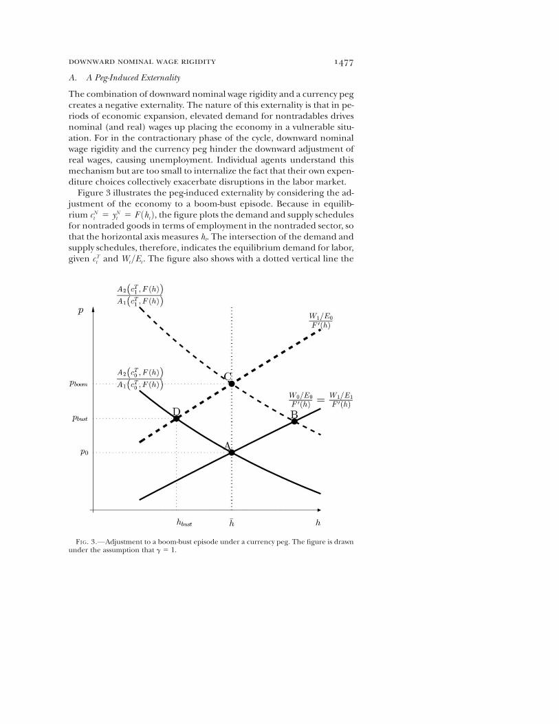
The combination of downward nominal wage rigidity and a currency pegcreates a negative externality. The nature of this externality is that in pe-riods of economic expansion, elevated demand for nontradables drivesnominal (and real) wages up placing the economy in a vulnerable situ-ation. For in the contractionary phase of the cycle, downward nominalwage rigidity and the currency peg hinder the downward adjustment ofreal wages, causing unemployment. Individual agents understand thismechanism but are too small to internalize the fact that their own expen-diture choices collectively exacerbate disruptions in the labor market.Figure 3 illustrates the peg-induced externality by considering the ad-

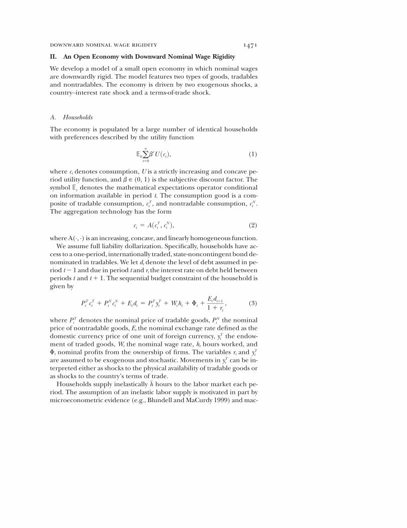
justment of the economy to a boom-bust episode. Because in equilib-rium cNt 5 yNt 5 F ðhtÞ, the figure plots the demand and supply schedulesfor nontraded goods in terms of employment in the nontraded sector, sothat the horizontal axis measures ht. The intersection of the demand andsupply schedules, therefore, indicates the equilibrium demand for labor,given cTt and Wt=Et . The figure also shows with a dotted vertical line the

FIG. 3.—Adjustment to a boom-bust episode under a currency peg. The figure is drawnunder the assumption that g 5 1.


labor supply, �h. Suppose that the initial position of the economy is at pointA, where the labor market is operating at full employment, ht 5 �h. Sup-pose that in response to a positive external shock, such as a decline inthe country interest rate, traded absorption increases from cT0 to cT1 >cT0 , causing the demand function to shift up and to the right. If nominalwages stayed unchanged, the new intersection of the demand and supplyschedules would occur at point B. However, at point B the demand for la-bor would exceed the available supply of labor �h. The excess demand forlabor drives up the nominal wage fromW0 toW1 > W0, causing the supplyschedule to shift up and to the left. The new intersection of the demandand supply schedules occurs at point C, where full employment is re-stored and the excess demand for labor has disappeared. The transitionfrom points A to C happens instantaneously because nominal wages areupwardly flexible. Although the economy is enjoying full employment,the increase in nominal wages is a harbinger of bad things to come.Suppose now that the positive external shock fades away and that, as

a consequence, absorption of tradables goes back to its normal level cT0 .The decline in cTt shifts the demand schedule back to its original position,indicated by the downward-sloping solid line.However, the economy doesnot return topointA. Becauseof downwardnominalwage rigidity, thenom-inal wage stays at W1, and because of the currency peg, the nominal ex-change rate remains at E0. As a result, the supply schedule continues tobe the broken upward-sloping line. The new intersection is at point D.There, the economy suffers involuntary unemployment equal to �h 2 hbust.If individual households could internalize the fact that consumptionboomslead to excessive wage growth and unemployment once the boom is over,theymight choose to restrain their appetite for tradable goods during theboom. This is the precise nature of the peg-induced externality.

B. Volatility and Mean Unemployment

The present model implies an endogenous connection between the am-plitude of the cycle and the average levels of involuntary unemploymentand output. This connection opens the door to large welfare gains fromoptimal stabilization policy and is rooted in the fact that under a currencypeg the economy adjusts asymmetrically to positive and negative externalshocks. The adjustment to positive external shocks is efficient, as nom-inal wages adjust upward to ensure that firms are on their labor demandschedule and households on their labor supply schedule. In sharp con-trast, the adjustment to negative external shocks is inefficient, as nominalwages fail to fall, forcing households off their labor supply schedule andgenerating involuntary unemployment. It follows that over the businesscycle, themodel economy fluctuates between periods of full employmentand an efficient level of production and periods of involuntary unem-


ployment and inefficiently low levels of production. Therefore, the aver-age levels of involuntary unemployment and nontraded output dependon the amplitude of the business cycle. That is, in this model, mean un-employment is increasing in the variance of the underlying shocks. Thisproperty of themodel obtains even if wage rigidity is symmetric (i.e., evenif nominal wages are equally rigid upwardly and downwardly). The reasonis that in the present model employment is determined by the smaller ofdemand and supply, as opposed to demand alone, as is the case in exist-ing sticky-wage models in the Erceg, Henderson, and Levin (2000) andGalí (2011) tradition. Asymmetric wage rigidity exacerbates the connec-tion between the volatility of the underlying shocks and the average levelof involuntary unemployment.

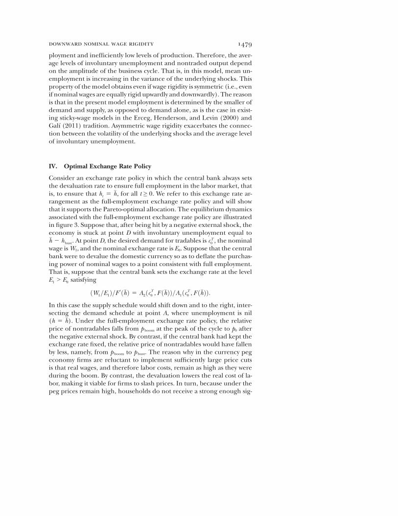
IV. Optimal Exchange Rate Policy

Consider an exchange rate policy in which the central bank always setsthe devaluation rate to ensure full employment in the labor market, thatis, to ensure that ht 5 �h, for all t ≥ 0. We refer to this exchange rate ar-rangement as the full-employment exchange rate policy and will showthat it supports the Pareto-optimal allocation. The equilibrium dynamicsassociated with the full-employment exchange rate policy are illustratedin figure 3. Suppose that, after being hit by a negative external shock, theeconomy is stuck at point D with involuntary unemployment equal to�h 2 hbust. At point D, the desired demand for tradables is cT0 , the nominalwage isW1, and the nominal exchange rate is E0. Suppose that the centralbank were to devalue the domestic currency so as to deflate the purchas-ing power of nominal wages to a point consistent with full employment.That is, suppose that the central bank sets the exchange rate at the levelE1 > E0 satisfying

ðW1=E1Þ=F 0ð�hÞ 5 A2ðcT0 , F ð�hÞÞ=A1ðcT0 , F ð�hÞÞ:In this case the supply schedule would shift down and to the right, inter-secting the demand schedule at point A, where unemployment is nil(h 5 �h). Under the full-employment exchange rate policy, the relativeprice of nontradables falls from pboom at the peak of the cycle to p0 afterthe negative external shock. By contrast, if the central bank had kept theexchange rate fixed, the relative price of nontradables would have fallenby less, namely, from pboom to p bust. The reason why in the currency pegeconomy firms are reluctant to implement sufficiently large price cutsis that real wages, and therefore labor costs, remain as high as they wereduring the boom. By contrast, the devaluation lowers the real cost of la-bor, making it viable for firms to slash prices. In turn, because under thepeg prices remain high, households do not receive a strong enough sig-


nal to switch expenditures away from tradables and toward nontradablesin a magnitude compatible with full employment.The full-employment policy amounts to setting the devaluation rate to

ensure that the real wage equals the full-employment real wage. We de-note the full-employment real wage by qðcTt Þ, where the function qðcTt Þ isgiven by

qðcTt Þ ;A2ðcTt , F ð�hÞÞA1ðcTt , F ð�hÞÞ

F 0ð�hÞ: (21)

The assumed properties of the aggregator function A ensure that thefunction qð�Þ is strictly increasing in cTt .The full-employment exchange rate policy stipulates that should the

nominal value of the full-employment real wage evaluated at last period’snominal exchange rate, qðcTt ÞEt21, fall below the lower bound gWt21, thenthe central bank devalues the domestic currency to ensure that qðcTt ÞEt ≥gWt21. That is, the devaluation rate makes the nominal wage,Wt, greaterthan or equal to its lower bound, gWt21, and at the same time guaranteesthat the real wage, wt, equals the full-employment real wage qðcTt Þ. In gen-eral, any exchange rate policy satisfying

et ≥ gwt21

qðcTt Þ(22)

ensures full employment at all times. All exchange rate policies pertain-ing to this family deliver the same real allocation and are therefore equiv-alent from a welfare point of view. Indeed, the real allocation induced bypolicies belonging to this family is Pareto optimal. The following propo-sition establishes these results.Proposition 1. Any exchange rate policy satisfying condition (22) is

consistent with a real allocation that exhibits full employment (ht 5 �h)at all dates and states and is Pareto optimal.Proof. See online appendix B.The Pareto-optimal allocation, denoted fcTot , do

t11g∞t50, is the solution to

the following value function problem:

voðyTt , rt , dtÞ 5 maxfcTt ,dt11g

fU ðAðcTt , F ð�hÞÞÞ 1 bEtvoðyTt11, rt11, dt11Þg (23)

subject to (10) and (11), where the function voðyTt , rt , dtÞ represents thewelfare level of the representative agent in state ðyTt , rt , dtÞ. The facts thatunder the optimal exchange rate policy aggregate dynamics can be de-scribed as the solution to a Bellman equation and that the past real wage,wt21, is not a relevant state variable in period t greatly facilitate the quan-titative characterization of the model’s predictions.


V. Optimal Fiscal Policy under a Currency Pegand Free Capital Mobility

Many observers have suggested the use of fiscal policy to ease the painsof currency pegs. However, advocates of active fiscal policy do not speakwith a single voice. Some argue that the right medicine is fiscal restraintvia tax increases and cuts in public expenditures. Others hold diametri-cally opposed views and argue that only widespread increases in govern-ment spending and tax cuts can offer pain relief. Our model suggeststhat both of these extreme views are misguided. Instead, the model sug-gests that the way to ease the pain of a currency peg by means of fiscalpolicy is more sophisticated in nature. In particular, optimal fiscal policyin the context of a currency peg can be implemented by a time-varyingwage subsidy at the firm level, financed with income taxes at the house-hold level.Suppose that the exchange rate is pegged (et 5 1) and that the govern-

ment subsidizes employment at the firm level at the rate tht and levies in-come taxes at the household level at the rate t

yt . The sequential budget

constraint of the household is then given by

cTt 1 ptcNt 1 dt 5 ð1 2 tyt ÞðyTt 1 wtht 1 ftÞ 1

dt11

1 1 rt, (24)

where ft ; Ft=Et denotes real profits in terms of tradables. Note thatthe proportional income tax t

yt is nondistorting, because households

take yTt , wtht , and ft as given. Consequently, the first-order conditionsof the household are as in the economy without income taxes (seeSec. II.A).With the wage subsidy, profits of firms expressed in terms of tradables

are given by ft 5 ptF ðhtÞ 2 ð1 2 tht Þwtht . The optimality condition forprofit maximization is

pt 5ð1 2 tht Þwt

F 0ðhtÞ: (25)

We assume that the government consumes no goods, starts with nodebt, and maintains a balanced budget period by period. Thus, its se-quential budget constraint is given by

tht wtht 5 tyt ðyTt 1 wtht 1 ftÞ : (26)

All other aspects of the model are as in the currency peg economy with-out taxes.The Pareto-optimal equilibrium can be supported under a currency

peg by setting the payroll subsidy tht as


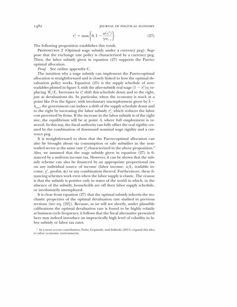
tht 5 max 0, 1 2qðcTt Þgwt21

� �: (27)

The following proposition establishes this result.Proposition 2 (Optimal wage subsidy under a currency peg). Sup-

pose that the exchange rate policy is characterized by a currency peg.Then, the labor subsidy given in equation (27) supports the Pareto-optimal allocation.Proof. See online appendix C.The intuition why a wage subsidy can implement the Pareto-optimal

allocation is straightforward and is closely linked to how the optimal de-valuation policy works. Equation (25) is the supply schedule of non-tradables plotted in figure 3, with the after-subsidy real wage ð1 2 tht Þwt re-placing Wt=Et . Increases in tht shift this schedule down and to the right,just as devaluations do. In particular, when the economy is stuck at apoint like D in the figure, with involuntary unemployment given by �h 2hbust, the government can induce a shift of the supply schedule down andto the right by increasing the labor subsidy tht , which reduces the laborcost perceived by firms. If the increase in the labor subsidy is of the rightsize, the equilibrium will be at point A, where full employment is re-stored. In this way, the fiscal authority can fully offset the real rigidity cre-ated by the combination of downward nominal wage rigidity and a cur-rency peg.It is straightforward to show that the Pareto-optimal allocation can

also be brought about via consumption or sale subsidies in the non-traded sector at the same rate tht characterized in the above proposition.2

Also, we assumed that the wage subsidy given in equation (27) is fi-nanced by a uniform income tax. However, it can be shown that the sub-sidy scheme can also be financed by an appropriate proportional taxon any individual source of income (labor income, wtht , tradable in-come, yTt , profits, ft) or any combination thereof. Furthermore, these fi-nancing schemes work even when the labor supply is elastic. The reasonis that the subsidy is positive only in states of the world in which, in theabsence of the subsidy, households are off their labor supply schedule,or involuntarily unemployed.It is clear from equation (27) that the optimal subsidy inherits the sto-

chastic properties of the optimal devaluation rate studied in previoussections (see eq. [22]). Because, as we will see shortly, under plausiblecalibrations the optimal devaluation rate is found to be highly volatileat business cycle frequency, it follows that the fiscal alternative presentedhere may indeed introduce an impractically high level of volatility in la-bor subsidy or labor tax rates.

2 In a more recent contribution, Farhi, Gopinath, and Itskhoki (2011) expand this ideato other economic environments.


VI. Optimal Capital Controls under a Currency Peg

In Section III.A, we established that the combination of a currency pegand downward nominal wage rigidity creates an externality. During epi-sodes of large capital inflows, nominal wages rise, making the economyvulnerable to unemployment once capital inflows dry up, as nominalwages cannot adjust downwardly to equilibrate the labor market. Individ-uals understand this source of fragility but are too small to do anythingabout it. Thus, under a currency peg and free capital mobility, the econ-omy overborrows during booms and suffers excessive unemploymentduring contractions. Consequently, the government has an incentive tointervene.In this section, we study the efficacy of capital controls in remedying

the peg-induced externality. We interpret the concept of capital controlsbroadly, as regulations of cross-border financial flows. For instance, theset of financial reform measures developed by the Basel Committee onBanking Supervision, known as Basel III, contemplates the use of pro-cyclical capital requirements for banks. This type of regulation is of in-terest because it tends to act like capital controls but without violatingpossible arrangements governing flows of financial capital across bor-ders, like those existing in the European Union.Specifically, we explore the possibility that the government acts pru-

dentially by imposing capital controls during booms. Such a policywould tend to curb capital inflows and in that way contain the rise innominal wages and limit the size of involuntary unemployment oncethe boom is over. Our approach is not to assume that capital controlsare prudential, but rather to investigate whether prudential capital con-trol policy emerges endogenously as a Ramsey-optimal outcome.The intuition for why the government may wish to use capital controls

in a prudential manner is illustrated in figure 4. Suppose that the econ-omy starts at point A. At that point traded consumption is equal to cT0 andthe economy enjoys full employment. Assume now that the economyexperiences a temporary decrease in the country interest rate followedby an increase, which causes a boom-bust response in cT. Assume thatin the absence of capital controls, consumption of tradables rises fromcT0 to cT1 > cT0 when the country interest rate falls and then declines backto cT0 once the country interest rate rises. As discussed earlier, in this casethe economy moves from point A to point C during the boom and thenfrom point C to point D in the bust. During the boom, nominal wagesrise from W0 to W1 > W0. In the bust, the economy experiences involun-tary unemployment in the amount of �h 2 hbust because real wages arestuck atW1=E0 and downward nominal wage rigidity in combination withthe currency peg prevents real wages from falling to a level consistentwith full employment.


Consider now the case in which the government implements capitalcontrol taxes in response to the initial interest rate decline and that as aresult of these taxes, the increase in traded consumption is smaller. Spe-cifically, assume that traded consumption now increases from cT0 to cT2 <cT1 . The demand for nontradables, shown with a broken downward-sloping line in figure 4, shifts up and to the right. As a result nominalwages increase to W2 and the nontradables supply schedule, shown witha broken upward-sloping line, shifts up and to the left. The new intersec-tion of the demand and supply schedules is at point C 0, where the econ-omy enjoys full employment. Because the shift in the demand schedulein the presence of capital controls is smaller than in their absence, nom-inal wages rise by less, that is, W2 < W1. Assume again that when the pos-itive external shock fades away, consumption of tradables falls back to cT0 .The resulting demand schedule is thus the same as the initial one, givenby the solid downward-sloping line in figure 4. The supply schedule (theupward-sloping broken line) does not shift because as a result of down-

FIG. 4.—Prudential capital control policy. The figure is drawn under the assumptionthat g 5 1.


ward nominal wage rigidity, nominal wages cannot decline, that is, wagesremain atW2, and as a result of the currency peg, the exchange rate can-not change, that is, it remains at E 0. The new intersection of the demandand supply schedules is at point D 0, where �h 2 h c

bust workers are involun-tarily unemployed. However, the level of unemployment at D 0 is lowerthan at D. It follows that by imposing capital controls in response to apositive external shock, that is to say, by imposing capital controls in aprudential manner, the government is able to reduce the amount of un-employment that occurs once the positive external shock is over.But this government intervention comes at the cost of bringing about

an inefficient allocation of traded consumption over time. For capitalcontrols distort the interest rate perceived by domestic households.The imposition of capital controls induces households not to take fulladvantage of the cheaper cost of borrowing during the boom and notto reduce their absorption of tradables sufficiently once the interest raterises. The figure illustrates the benefits in terms of lower unemploymentthat capital controls can bring. But the figure does not capture the costsin terms of a suboptimal time path of tradable consumption. To analyzethe trade-off between less unemployment and an inefficient allocationof traded consumption over time, we next characterize Ramsey-optimalcapital control policies more formally.Assume that the government taxes external debt at the proportional

rate tdt and rebates this source of revenue via a proportional incomesubsidy denoted t

yt . The budget constraint of the household is then

given by

cTt 1 ptcNt 1 dt 5 ð1 1 tyt ÞðyTt 1 wtht 1 ftÞ 1

ð1 2 tdt Þdt11

1 1 rt:

We note again that because all sources of income—yTt , wtht , and ft—aretaken as exogenous by the household, the income subsidy used to rebatethe revenues from capital controls is nondistorting. The introduction ofa capital control tax changes the household’s first-order condition forholdings of foreign assets to

lt

1 2 tdt1 1 rt

5 bEtlt11 1 mt : (28)

According to this expression, the effective gross interest rate ondebt holdings between periods t and t 1 1 perceived by households isð1 1 rtÞ=ð1 2 tdt Þ, which is greater than the gross country interest rate,1 1 rt, when the government imposes capital controls, that is, when tdt >0. Observe that the effective interest rate, ð1 1 rtÞ=ð1 2 tdt Þ, like thecountry interest rate, 1 1 rt, is in the information set of period t.


Thus, the capital control policy considered here preserves the state-noncontingent nature of external debt.The government is assumed to be benevolent and to be endowed with

full commitment. We therefore refer to the government as the Ramseyplanner. We assume that the government pegs the currency and cannotuse labor subsidies of the type studied in Section V. The budget con-straint of the government is therefore given by

tyt ðyTt 1 wtht 1 ftÞ 5tdt dt11

1 1 rt: (29)

The policy variable tdt can take positive or negative values. In the formercase it represents a tax on capital inflows and in the latter a subsidy.Because the monetary authority pegs the currency at all times, equilib-

rium conditions (17) and (19) become, respectively,

wt ≥ gwt21 (30)

and

ðht 2 �hÞ wt 2 gwt21ð Þ 5 0: (31)

We then have the following definition of equilibrium in the economywith capital controls.Definition 2 (Equilibrium with capital controls and a currency peg).

Under capital controls and a currency peg, an equilibrium is a set of sto-chastic processes fcTt , ht , wt , dt11, lt , mt , t

ytg∞

t50 satisfying (10)–(14), (16),(18), and (28)–(31), given a capital control policy ftdt g∞

t50, initial condi-tions w21 and d0, and exogenous stochastic processes frt , yTt g∞

t50.The Ramsey planner’s optimization problem consists in choosing a

tax scheme ftdt g to maximize the household’s lifetime utility function(1) subject to the equilibrium conditions listed in definition 2. The strat-egy we follow to characterize the Ramsey allocation is to drop from theRamsey planner’s problem all constraints except for (10), (11), (16),(18), and (30) and then show that the solution to this less constrainedproblem satisfies the omitted constraints.Accordingly, the less constrained Ramsey problem (LCP) is given by

maxfcTt ,dt11,ht ,wtg∞

t50

E0o∞

t50

btU ðAðcTt , F ðhtÞÞÞ

subject to (10), (11), (16), (18), and (30), given d0, w21, and the stochas-tic processes frt , yTt g∞

t50.We now show that the allocation fcTt , dt11, ht , wtg∞

t50 that solves the LCPsatisfies the constraints of the original Ramsey problem listed in defini-tion 2. To see this, use the LCP allocation to construct lt to satisfy (14).


Next, set mt 5 0 for all t.3 It follows that (12) and (13) are satisfied. Nowconstruct tdt to satisfy (28) and t

yt to satisfy (29). It remains to be shown

that the allocation that solves the LCP satisfies the slackness condition(31). To see that this is the case, consider the following proof by contra-diction. Suppose, contrary to what we wish to show, that the solution tothe LCP implies ht < �h and wt > gwt21 at some date t 0 ≥ 0. Consider now aperturbation to the allocation that solves the LCP consisting in a smallincrease in hours at time t 0 from ht 0 to ~ht 0 ≤ �h. Clearly, this perturbationdoes not violate the resource constraint (10), since hours do not enterin this equation. From (16) we have that the real wage falls to

~wt 0 ;A2ðcTt 0 , F ð~ht 0 ÞÞA1ðcTt 0 , F ð~ht 0 ÞÞ

F 0ð~ht 0 Þ < wt 0

(recall that the expression in the middle is decreasing in hours). Be-cause A1, A2, and F 0 are continuous functions, expression (30) is satisfiedprovided that the increase in hours is sufficiently small. In period t 0 1 1,restriction (30) is satisfied because ~wt 0 < wt 0 . We have therefore estab-lished that the perturbed allocation satisfies the restrictions of theLCP. Finally, the perturbation is clearly welfare increasing because it raisesthe consumption of nontradables in period t 0 without affecting the con-sumption of tradables in any period or the consumption of nontradablesin any period other than t 0. It follows that an allocation that does not sat-isfy the slackness condition (31) cannot be a solution to the LCP. Thiscompletes the proof that the allocation that solves the LCP is also feasi-ble in the Ramsey planner’s problem. It follows that the allocation thatsolves the LCP is indeed the Ramsey-optimal allocation. We summarizethis result in the following proposition.Proposition 3 (Optimal capital controls under a currency peg). Let

fcT c

t , dct11, h

ct , w

ct g∞

t50 be the allocation associated with the Ramsey-optimalcapital control policy in the economy with a currency peg. Then fcT c

t ,dct11, h

ct , w

ct g∞

t50 is the solution to the problem of maximizing (1) subjectto (10), (11), (16), (18), and (30), given d0, w21, and the stochastic pro-cesses frt , yTt g∞

t50.A corollary of this proposition is that one can characterize the Ramsey

allocation as the solution to the following Bellman equation problem:

vcðyTt , rt , dt , wt21Þ 5 max½U ðAðcTt , F ðhtÞÞ1 bEtv

cðyTt11, rt11, dt11, wtÞ�(32)

3 Note that in states in which the allocation calls for setting dt11 < �d, mt must be chosen tobe zero. However, in states in which the Ramsey allocation yields dt11 5 �d, mt need not bechosen to be zero. In these states, any positive value of mt could be supported in the decen-tralization of the Ramsey equilibrium. Of course, in this case, tdt will depend on the chosenvalue of mt. In particular, tdt will be strictly decreasing in the arbitrarily chosen value of mt.


subject to (10), (11), (16), (18), and (30), where vcðyTt , rt , dt , wt21Þ de-notes the value function of the representative household. We exploit thisformulation of the Ramsey problem in our quantitative analysis.The allocation induced by the Ramsey-optimal capital control policy

can also be supported through consumption taxes. Specifically, assumethat instead of taxing external debt, the government taxes total con-sumption expenditures, cTt 1 ptc

Nt , at the rate tct21, so that the after-tax

cost of consumption in period t is ðcTt 1 ptcNt Þð1 1 tct21Þ. The consump-

tion tax rate is determined one period in advance. That is, in period tthe government announces the tax rate on consumption expendituresthat will be in effect in period t 1 1. One can show that the Ramsey al-location can be supported by a consumption tax process of the form 1 1tct 5 ð1 2 tdt Þð1 1 tct21Þ, for any initial condition tc21 > 21, where tdt rep-resents the Ramsey-optimal tax rate on external debt. According to thisexpression, if the Ramsey-optimal capital control tax in period t is posi-tive (the planner is discouraging borrowing), then the associated Ramsey-optimal consumption tax scheme stipulates a decline in the consumptiontax rate between periods t and t 1 1 so as to induce households to post-pone consumption. Suppose now that the optimal capital control tax ispositive on average, which we will show is the case in the calibrated econ-omy studied in Section IX. Then, it is clear from the above formula thatthe associated optimal consumption tax rate converges asymptotically to asubsidy of 100 percent of consumption expenditure, or tct →21. This sug-gests an advantage of capital control taxes over consumption taxes froma practical point of view.We also note that the model with Ramsey-optimal capital controls is

equivalent to one in which a benevolent government chooses the levelof external debt and households cannot participate in financial marketsbut are hand-to-mouth agents. In this formulation, households receive atransfer from the government each period and their choice is limited tothe allocation of expenditure between tradable and nontradable goods.The government then chooses the aggregate level of external debt tak-ing into account the externality created by the combination of down-ward nominal wage rigidity and a currency peg.

VII. The Optimality of Prudential Capital Controlsunder a Currency Peg: An Analytical Example

In this section, we present an analytical example showing the prudentialnature of optimal capital controls. We characterize the optimal capitalcontrol policy in response to a temporary decline in the interest rateand show that the Ramsey policy calls for an increase in capital controltaxes while the interest rate is low. This intervention discourages capitalinflows, thereby attenuating the expansion in tradable absorption. The


example highlights the cost of capital controls, which take the form of aninefficient intertemporal allocation of consumption, and their benefits,which take the form of lower involuntary unemployment once the boomis over.Consider an economy like the one studied thus far in which the gov-

ernment pegs the nominal exchange rate. Assume that preferences aregiven by U ðctÞ 5 lnðctÞ and AðcTt , cNt Þ 5 cTt c

Nt . The technology for pro-

ducing nontradable goods is F ðhtÞ 5 hat , with a ∈ (0, 1). Assume that the

economy starts period 0 with no outstanding debt, d05 0, that the endow-ment of tradables, yT, is constant over time, and that the real wage in pe-riod21 equals ayT. Consider a situation in which the economy is subjectto a temporary interest rate decline in period 0. Specifically, supposethat r0 5 r and rt 5 r > r for t ≠ 0. This interest rate shock is assumedto be unanticipated. Finally, assume that bð1 1 r Þ 5 1, that g 5 1,and that �h 5 1. The economy is assumed to have been at a full-employment equilibriumprior to the interest rate shock, with dt5 0, cTt 5yT , and ht 5 cNt 5 1 for t < 0.In online appendix D, we show that under optimal capital controls, all

variables are constant over time starting in period 1. The constancy of allvariables is a consequence of the fact that after period 0 the economy suf-fers no further disturbances and of the assumptions that b(1 1 r) and g

are both equal to unity. The former parameter restriction ensures theconstancy of tradable consumption and the latter the constancy of thereal wage. This result implies that capital controls are zero starting in pe-riod 1. Online appendix D further establishes that in period 0 thechange in tradable consumption is nonnegative, that is, cT0 ≥ yT , andthus capital inflows are nonnegative, that is, d1 ≥ d0 5 0. Intuitively,the fall in the interest rate encourages international borrowing and con-sumption. In period 0, the economy enjoys full employment, h0 5 1. Thisis natural, since low interest rates stimulate aggregate demand. Finally,online appendix D shows that starting in period 1, employment is givenby ht 5 cT1 =c

T0 ≤ 1, for t ≥ 1. This expression says that unemployment is

increasing in the contraction in aggregate demand in period 1. Unem-ployment is persistent because wages cannot fall (g 5 1).With these results in hand, the Ramsey-optimal capital control prob-

lem simplifies to

maxfcT0 ,cT1 ,d1g

ln cT0 1b

1 2 bln cT1 1

ab

1 2 bðln cT1 2 ln cT0 Þ

� �

subject to d1 ≥ 0, cT0 5 yT 1 ½d1=ð1 1 r Þ�, and cT1 5 yT 2 ½rd1=ð1 1 rÞ�.The optimality conditions associated with this problem are the abovethree constraints,


1

1 1 r

1

cT02 b

1

cT12 ab

1

cT11

1 1 r

rð1 1 rÞ1

cT0

� �≤ 0, (33)

and the slackness condition

1

1 1 r

1

cT02 b

1

cT12 ab

1

cT11

1 1 r

r ð1 1 r Þ1

cT0

24

35

8<:

9=;d1 5 0:

The first two terms of optimality condition (33) represent the trade-offthat the representative household would face in an unregulated economyin deciding whether to take on an additional unit of debt in period 0. Anadditional unit of debt allows the household to consume 1=ð1 1 r Þ unitsof goods in period 0. In period 1, the household must repay one unit ofconsumption to cancel the debt assumed in period 0. We refer to thefirst two terms as the private marginal utility of debt. The third termin (33) captures the externality created by the combination of downwardnominal wage rigidity and a currency peg. It reflects the Ramsey plan-ner’s internalization of the fact that changes in consumption affect un-employment (recall that ht 5 cT1 =c

T0 for all t ≥ 1). This is an equilibrium

effect that is not taken into account by individual consumers. We refer tothe sum of the three terms as the social marginal utility of debt. Since thethird term is negative, we have that the social marginal utility of debt isalways lower than its private counterpart.4

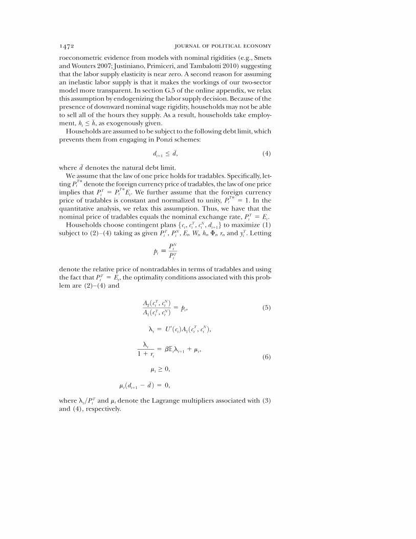
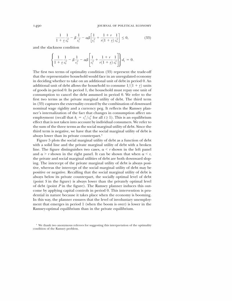
Figure 5 plots the social marginal utility of debt as a function of debtwith a solid line and the private marginal utility of debt with a brokenline. The figure distinguishes two cases, a < r shown in the left paneland a > r shown in the right panel. It can be shown that when a < r,the private and social marginal utilities of debt are both downward slop-ing. The intercept of the private marginal utility of debt is always posi-tive, whereas the intercept of the social marginal utility of debt may bepositive or negative. Recalling that the social marginal utility of debt isalways below its private counterpart, the socially optimal level of debt(point S in the figure) is always lower than the privately optimal levelof debt (point P in the figure). The Ramsey planner induces this out-come by applying capital controls in period 0. This intervention is pru-dential in nature because it takes place when the economy is booming.In this way, the planner ensures that the level of involuntary unemploy-ment that emerges in period 1 (when the boom is over) is lower in theRamsey-optimal equilibrium than in the private equilibrium.

4 We thank two anonymous referees for suggesting this interpretation of the optimalitycondition of the Ramsey problem.


Consider now the case a >r shown in the right panel of figure 5. In thiscase the social marginal utility of debt is negative for all nonnegative val-ues of debt. Thus, the socially optimal response to the decline in the in-terest rate is a corner solution featuring d1 5 0 (point S in the figure).The Ramsey planner imposes capital controls such that the privately per-ceived (after-tax) interest rate ð1 1 rÞ=ð1 2 td0Þ equals 1 1 r.5

Thus, private households have no incentives to alter their consump-tion plans.6 The benefit of this strong distortion of the intertemporal al-location of tradable absorption is full employment at all times. On theother hand, the private marginal utility of debt continues to be down-ward sloping with a positive intercept. As a consequence, the privatelyoptimal level of debt (point P in the figure) is always positive and thushigher than the socially optimal level.7

In the case in which a > r, the optimal capital control policy resolvesthe trade-off between intertemporal distortions and static distortions en-tirely in favor of eliminating all static distortions, that is, full employment

FIG. 5.—Private and social marginal utility of debt. Color version available as an onlineenhancement.

5 Implementing the same real allocation via consumption taxes instead of capital con-trols would require a permanent consumption subsidy at the gross rate ðr 2 r Þ=ð1 1 rÞstarting in period 1.

6 The change in the world interest rate does not generate a wealth effect because thedesired net asset position prior to the change in the interest rate was nil.

7 The intuition for why a > r is a sufficient condition for the corner solution of no in-crease in debt in response to a decline in the interest rate is as follows. An increase in debtimplies a fall in employment of at least 1=cT0 for all t ≥ 1 (recall that ht 5 cT1 =c

T0 ). This is

equivalent to a decline in nontradable output of a=cT0 for all t ≥ 1. The value of this amountof nontradables in terms of tradables is a since the relative price of nontradables in termsof tradables is cT0 . The present discounted value of a stream of a units of tradables is ap-proximately a/r. Thus, if this value is larger than unity (the increase in tradable consump-tion afforded by a unit increase in debt in period 0), the planner will never choose to in-crease debt in period 0.


at all times. In the case in which a < r, the trade-off is resolved in a morebalanced fashion. The optimal capital control policy consists in reducing(but not eliminating) inefficient unemployment and distorts (althoughless strongly) the intertemporal allocation of consumption. As we will seeshortly, the thrust of these findings carries over to richer economic envi-ronments.

VIII. Evidence on Downward Nominal Wage Rigidityand Estimates of g

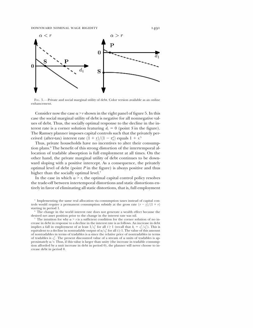
The central friction in the present theoretical framework is downwardnominal wage rigidity, embodied in the parameter g. There is abundantempirical evidence on downward nominal wage rigidity stemmingmostly from developed countries.8 In this section we present novel evi-dence from emerging countries and propose an empirical strategy foridentifying the wage rigidity parameter g. The strategy consists in observ-ing the behavior of nominal wages during periods of rising unemploy-ment and low inflation. We focus on episodes in which an economy un-dergoing a severe recession keeps the nominal exchange rate fixed. Twoprominent examples are Argentina during the second half of the Con-vertibility Plan (1998–2001) and the periphery of Europe during theGreat Recession of 2008.Figure 6 displays the nominal exchange rate, subemployment (de-

fined as the sum of unemployment and underemployment), nominal(peso) wages, and real (dollar) wages for Argentina during the period1996–2006. The subperiod 1998–2001 is of particular interest becauseduring that time the Argentine central bank was holding on to the cur-rency peg in spite of the fact that the economy was undergoing a severecontraction and both unemployment and underemployment were in asteep ascent. In the context of a flexible-wage model, one would expectthat the rise in unemployment would be associated with falling realwages. With the nominal exchange rate pegged, the fall in real wagesmust materialize through nominal wage deflation. However, during thisperiod, the nominal hourly wage never fell. Indeed, it increased from7.87 pesos in 1998 to 8.14 pesos in 2001. The present model predicts thatwith rising unemployment, the lower bound on nominal wages shouldbe binding, and therefore, g should equal the gross growth rate of nom-

8 See, e.g., Gottschalk (2005) for the United States from 1986 to 1993; Barattieri, Basu,and Gottschalk (2010) for the United States from 1996 to 1999; Daly, Hobijn, and Lucking(2012) for the United States during the Great Recession of 2008; Eichengreen and Sachs(1985) for western Europe during the Great Depression of 1929; Holden and Wulfsberg(2008) for OECD countries; Fortin (1996) for Canada; Kuroda and Yamamoto (2003)for Japan; and Fehr and Goette (2005) for Switzerland. Kaur (2012) presents evidencefrom informal labor markets in rural India.


inal wages. An estimate of the parameter g can then be constructed asthe average quarterly growth rate of nominal wages over the 3-year pe-riod considered, that is, g 5 ðW2001=W1998Þ1=12. This yields a value of g of1.0028.In order for this estimate of g to represent an appropriate measure of

wage rigidity in the context of the theoretical model, it must be adjustedto account for the fact that our model abstracts from foreign inflationand long-run productivity growth. To carry out this adjustment, we usethe growth rate of the US GDP deflator as a proxy for foreign inflation.Between 1998 and 2001, the US GDP deflator grew by 1.77 percentper year on average. We set the long-run growth rate in Argentina at1.07 percent per year, to match the average growth rate of Argentineper capita real GDP over the period 1900–2005 reported in García-Cicco,Pancrazi, and Uribe (2010). The adjusted value of g is then given by1:0028=ð1:0107 � 1:0177Þ1=4 5 0:9958. This value of g means that realwages can fall frictionlessly by 1.7 percent per year.

FIG. 6.—Nominal wages and unemployment in Argentina, 1996–2006. Own calculationsbased on nominal exchange rate and nominal wage data from the Bureau of Labor Statis-tics and subemployment data from Instituto Nacional de Estadistica y Censos de Argentina.The data are provided with the online materials of this paper.


We note additionally that the fact that Argentine real wages fell sig-nificantly and persistently after the devaluation of 2002 (bottom-rightpanel of fig. 6) suggests that the 1998–2001 period was one of censoredwage deflation, which further strengthens the view that nominal wagessuffer from downward inflexibility.Finally, we note that during the 1998–2001 Argentine contraction,

consumer prices, unlike nominal wages, did fall significantly. The con-sumer price index (CPI) rate of inflation was, on average,20.86 percentper year over the period 1998–2001. It follows that real wages rose notonly in dollar terms but also in terms of CPI units. Incidentally, this ev-idence provides some support for our assumption that downward nom-inal rigidities are less stringent for product prices than for factor prices.The second episode from the emerging-market world that we use to

infer the value of g is the Great Recession of 2008 in the periphery ofEurope. Table 1 presents an estimate of g for 12 European economiesthat are either on the euro or pegging to the euro. The table showsthe unemployment rate in 2008:Q1 and 2011:Q2. The starting pointof this period corresponds to the beginning of the Great Recession inEurope according to the Centre for Economic Policy Research Euro AreaBusiness Cycle Dating Committee. The 2008 crisis caused unemploymentrates to rise sharply across all 12 countries. The table also displays the to-tal growth of nominal hourly labor cost in manufacturing, construction,and services (including the public sector) over the 13-quarter period2008:Q1–2011:Q2.9 Despite the large surge in unemployment, nominalwages grew in most countries, and in those in which they fell, the declinewas modest. The implied value of g, shown in the last column of table 1, isgiven by the average growth rate of nominal wages over the period consid-ered, that is, g 5 ðW2011:Q2=W2008:Q1Þ1=13. The estimated values of g rangefrom 0.996 for Lithuania to 1.028 for Bulgaria.To adjust g for foreign inflation, we use the fact that over the 13-quarter

sample period considered in table 1, inflation in Germany was 3.6 per-cent, or about 0.3 percent per quarter. To adjust for long-run growth,we use the average growth rate of per capita output in the southern pe-riphery of Europe of 1.2 percent per year or 0.3 percent per quarter.10 Al-lowing for these effects suggests an adjusted estimate of g in the interval[0.990, 1.022].Taken together, the evidence examined in this section suggests that

downward nominal wage rigidity is pervasive in emerging countriesand that during low-inflation periods a conservative estimate of g is

9 The public sector is not included for Spain because of data limitations.10 This figure corresponds to the average growth rate of per capita real GDP in Greece,

Spain, Portugal, and Italy over the period 1990–2011 according to the World DevelopmentIndicators.


0.99 at a quarterly frequency. This value implies that nominal wages candecline up to 4 percent per year.

IX. Quantitative Analysis

In this section we characterize quantitatively the behavior of the econ-omy under the alternative policy arrangements analyzed theoretically inSections III–VI.

A. Calibration

We calibrate the model at a quarterly frequency using data from Argen-tina as shown in table 2. We estimate a bivariate AR(1) process for the

TABLE 1Unemployment, Nominal Wages, and g: Evidence from the Euro Zone

Unemployment Rate Wage Growth

Country 2008:Q1 (%) 2011:Q2 (%)W2011:Q2/W2008:Q2

Implied

Value of g

Bulgaria 6.1 11.3 43.3 1.028Cyprus 3.8 6.9 10.7 1.008Estonia 4.1 12.8 2.5 1.002Greece 7.8 16.7 22.3 .9982Ireland 4.9 14.3 .5 1.0004Italy 6.4 8.2 10.0 1.007Lithuania 4.1 15.6 25.1 .996Latvia 6.1 16.2 2.6 .9995Portugal 8.3 12.5 1.91 1.001Spain 9.2 20.8 8.0 1.006Slovenia 4.7 7.9 12.5 1.009Slovakia 10.2 13.3 13.4 1.010

Note.—Own calculations are based on data from Eurostat. The variableW is an index of nominal average hourly labor cost in manufacturing, con-struction, and services. Unemployment is the economywide unemploymentrate. The data are provided with the online materials of this paper.

TABLE 2Baseline Calibration

Parameter Value Description

g .99 Degree of downward nominal wage rigidityj 5 Inverse of intertemporal elasticity of consumptionyT 1 Steady-state tradable output�h 1 Labor endowmenta .26 Share of tradablesy .44 Elasticity of substitution between tradables and

nontradablesa .75 Labor share in nontraded sectorb .9375 Quarterly subjective discount factor


exogenous driving forces ðyTt , rtÞ by ordinary least squares using data overthe period 1983:Q1 to 2001:Q4. The empirical measure of yTt is the cycli-cal component of Argentine GDP in agriculture, forestry, fishing, min-ing, and manufacturing at 1993 prices. We measure the country-specificreal interest rate as the sum of the Emerging Market Bond Index 1spread for Argentina and the 90-day US Treasury Bill rate, deflated usinga measure of expected dollar inflation.11 Online appendix E providesfurther details on the data sources. The estimated process is

ln yTt

ln1 1 rt1 1 r

264

375 5

0:7901 21:3570

20:0104 0:8638

" # ln yTt21

ln1 1 rt21

1 1 r

264

375 1 et ;

et ∼ N ∅,0:0012346 20:0000776

20:0000776 0:0000401

" # !,

(34)

and r5 0.0316. According to these estimates, both ln yTt and rt are highlyvolatile, with unconditional standard deviations of 12.2 percent and1.7 percent per quarter, respectively. The unconditional contemporane-ous correlation between ln yTt and rt is high and negative at20.86, imply-ing that borrowing conditions for debtors tend to deteriorate at thewrong time, namely, when output is low. The estimated joint auto-regressive process implies that both traded output and the real interestrate are persistent, with first-order autocorrelations of .95 and .93, re-spectively. The estimated value of the steady-state real interest rate ishigh at 3.16 percent per quarter, or 13.2 percent per year.We set g at 0.99, the lowest of the cross-country estimates reported in

Section VIII. This value imposes the least amount of wage rigidity de-tected in the Argentine and European data. This value of g means thatnominal wages can fall by up to 4 percent per year. Online appendix G.4considers the case of g 5 0.98, which allows nominal wages to fall by upto 8 percent per year.We assume the constant relative risk aversion form U ðcÞ 5 ðc12j 2

1Þ=ð1 2 jÞ for the period utility function, the constant elasticity of sub-stitution form

AðcT , cN Þ 5 aðcT Þ12ð1=yÞ 1 ð1 2 aÞðcN Þ12ð1=yÞ� y=ðy21Þ

for the aggregator function, and the isoelastic form F ðhÞ 5 ha for theproduction function of nontradables. Reinhart and Végh (1995) esti-

11 The country-specific interest rate reflects the fact that, in general, each country bor-rows at a different interest rate. The country interest rate captures factors such as country-specific repayment risk. These idiosyncratic interest rate differentials are present even forcountries that are part of a monetary union, such as the members of the euro zone.


mate the intertemporal elasticity of substitution to be 0.21 using Argen-tine quarterly data. We therefore set j equal to 5. Online appendix G.3considers a value of j close to 2. We set �h equal to unity. Then, if thesteady-state trade balance to output ratio is small, as is the case in Argen-tina, the parameter a is approximately equal to the share of traded out-put in total output.12 The share of traded output observed in Argentinedata over the period 1980:Q1–2010:Q1 is 26 percent; hence we set a 50.26. Using time-series data for Argentina over the period 1993:Q1–2001:Q3, González Rozada et al. (2004) estimate the elasticity of substitu-tion between traded and nontraded consumption, y, to be 0.44. This es-timate is consistent with the cross-country estimates of Stockman andTesar (1995). These authors include in their estimation both developedand developing countries. Restricting the sample to include only devel-oping countries yields a value of y of 0.43 (see Akinci 2011). FollowingUribe’s (1997) evidence on the size of the labor share in the nontradedsector in Argentina, we set a equal to 0.75.We set �d at the natural debt limit, which we define as the level of ex-

ternal debt that can be supported with zero tradable consumption whenthe household perpetually receives the lowest possible realization oftradable endowment, yT

min

, and faces the highest possible realization ofthe interest rate, rmax. Formally, �d ; yT

minð1 1 r maxÞ=r max, which in the pres-ent calibration equals 8.34.Finally, we set b to match an average foreign-debt-to-output ratio of

26 percent per year, a value in line with that reported for Argentina overour calibration period by Lane and Milesi-Ferretti (2007). The cali-brated value of b is small relative to those typically used to calibrateclosed-economy models or open-economy models with a stationarity-inducing feature as described in Schmitt-Grohé and Uribe (2003). Butlow values of b are more common in open-economy models that donot include a stationarity-inducing device.

B. Approximating Equilibrium Dynamics

Here we sketch the numerical solution methods we employ to approxi-mate the equilibrium dynamics under the three policy arrangements weconsider, namely, in ascending order of computational complexity, theoptimal exchange rate policy, a currency peg with optimal capital con-trols, and a currency peg with free capital mobility.Under all three policy arrangements, the approximation involves

discretizing the state space. We discretize the exogenous AR(1) process

12 The parameter a is approximately equal to the share of tradable output in total out-put even though y ≠ 1 because, if the trade balance is near zero, traded output is nearunity, and hours are close to �h 5 1, we have that cN 5 yN ≈ cT ≈ yT ≈ 1 and p ≈ ð1 2 aÞ=a,which implies that yT=ðyT 1 pyN Þ ≈ a.


(34) using 21 equally spaced points for ln yTt in the interval ±0.3858 and11 equally spaced points for lnð1 1 rtÞ=ð1 1 r Þ in the interval ±0.0539.13

The transition probability matrix of the exogenous driving process istherefore of size 231� 231.14 To compute this matrix, we follow the algo-rithm described in Schmitt-Grohé and Uribe (2009). The resulting tran-sition probability matrix captures well the covariance matrices of order 0and 1.To discretize the endogenous state dt, we use 501 equally spaced points.

We fix the upper bound of the debt grid at 8, which is close to �d 5 8:34,and the lower bound at 25.When the exchange rate policy takes the form of a currency peg

(whether combined with free capital mobility or with capital controls), asecond endogenous state emerges, namely, past real wages, wt21. We dis-cretize this state using a grid of 500 equally spaced points for the logarithmof wt21. We set the lowest grid value of wt21 at 0.5 and the highest at 5.3.The equilibrium dynamics under the optimal exchange rate policy are

obtained from the solution to the value function problem given by thefunctional equation (23) and the constraints (8), (10), and (11). We nu-merically approximate this solution by applying the method of valuefunction iteration over a discretized state space. Under the optimal ex-change rate policy, the state of the economy in period t ≥ 0 is the tripletfyTt , rt , dtg.The equilibrium dynamics under a currency peg with the optimal cap-

ital control policy can be approximated by solving the functional equa-tion (32) subject to (10), (11), (16), (18), and (30). Approximatingthe equilibrium dynamics in this environment is more demanding thandoing so under the optimal exchange rate policy because the formerproblem includes an additional state variable, namely, wt21. We numeri-cally approximate the equilibrium dynamics by applying the method ofvalue function iteration over a discretized state space. The state of theeconomy in period t ≥ 0 consists of the quadruplet fyTt , rt , dt , wt21g.The task of approximating the equilibrium dynamics becomes even

more challenging under a currency peg with free capital mobility. Asin the case of a currency peg with optimal capital controls, there are fourstate variables, yTt , rt, dt, and wt21. However, under a currency peg with freecapital mobility, aggregate dynamics cannot be cast in terms of a Bell-man equation without introducing additional state variables, such asthe individual level of debt, which households perceive as distinct fromits aggregate counterpart. We therefore approximate the solution by

13 The lengths of these intervals are 2 � ffiffiffiffiffi10

ptimes the standard deviation of each vari-

able.14 Because some pairs ðyTt , rtÞ occur with probability zero, the transition probability ma-

trix can be reduced to one of dimension 145 � 145.


Euler equation iteration over a discretized version of the state spaceðyTt , rt , dt , wt21Þ. Online appendix F describes our numerical algorithmin more detail. Matlab codes are provided with the online materials ofthis paper.

C. Boom-Bust Cycles

We define a boom-bust episode as a situation in which tradable output, yTt ,is at or below trend in period 0, at least one standard deviation abovetrend in period 10, and at least one standard deviation below trend inperiod 20. This definition is motivated by the contraction in aggregateactivity observed in Argentina in 2001. We simulate the model economyfor 20 million periods and select all subperiods that satisfy our definitionof a boom-bust episode. We then average across these episodes.The top two panels of figure 7 display the dynamics of the two exoge-

nous driving forces, tradable output and the country interest rate. Becauseour estimate of the exogenous driving forces features a high negative cor-relation between traded output and the country interest rate, a boom-bustepisode can also be interpreted as one in which the interest rate falls onestandard deviation below mean over a period of 10 quarters and thenrises to one standard deviation above mean in the following 10 quarters.The middle and bottom panels of the figure depict the model’s pre-

dictions during the boom-bust cycle. Solid lines correspond to the econ-omy with a currency peg and free capital mobility, broken lines to theeconomy with a currency peg and optimal capital controls, and dottedlines to the economy with the optimal exchange rate policy.The middle-left panel of the figure shows that the optimal capital con-

trol policy is prudential. Capital controls increase significantly duringthe expansionary phase of the cycle, from about 2 percent at the begin-ning of the episode to 6 percent at the peak of the cycle. During thecontractionary phase of the cycle, capital controls are drastically relaxed.Indeed at the bottom of the crisis, capital inflows are actually subsidizedat a rate of about 2 percent. The sharp increase in capital controls duringthe expansionary phase of the cycle puts sand in the wheels of capitalinflows, thereby restraining the boom in tradable consumption (seethe bottom-right panel). Under a peg with free capital mobility, duringthe boom, tradable consumption increases significantly more than un-der the optimal capital control policy. In the contractionary phase, thefiscal authority incentivates spending in tradables by subsidizing capitalinflows. As a result consumption falls by much less in the regulated econ-omy than it does in the unregulated one. During the recession, the op-timal capital control policy, far from calling for austerity in the form ofsevere cuts in tradable consumption, supports this type of expenditure.That is, the capital control policy stabilizes the absorption of tradable


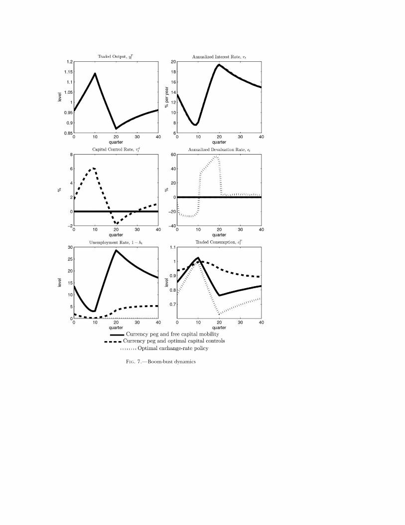
FIG. 7.—Boom-bust dynamics

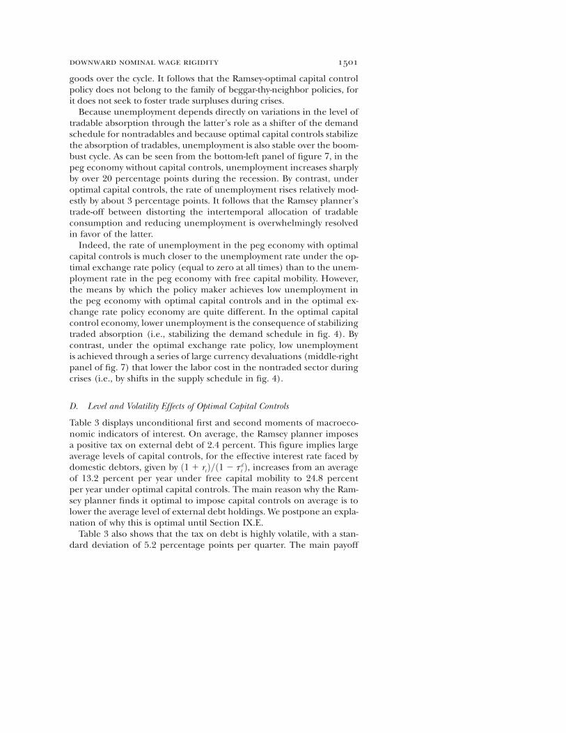
goods over the cycle. It follows that the Ramsey-optimal capital controlpolicy does not belong to the family of beggar-thy-neighbor policies, forit does not seek to foster trade surpluses during crises.Because unemployment depends directly on variations in the level of

tradable absorption through the latter’s role as a shifter of the demandschedule for nontradables and because optimal capital controls stabilizethe absorption of tradables, unemployment is also stable over the boom-bust cycle. As can be seen from the bottom-left panel of figure 7, in thepeg economy without capital controls, unemployment increases sharplyby over 20 percentage points during the recession. By contrast, underoptimal capital controls, the rate of unemployment rises relatively mod-estly by about 3 percentage points. It follows that the Ramsey planner’strade-off between distorting the intertemporal allocation of tradableconsumption and reducing unemployment is overwhelmingly resolvedin favor of the latter.Indeed, the rate of unemployment in the peg economy with optimal

capital controls is much closer to the unemployment rate under the op-timal exchange rate policy (equal to zero at all times) than to the unem-ployment rate in the peg economy with free capital mobility. However,the means by which the policy maker achieves low unemployment inthe peg economy with optimal capital controls and in the optimal ex-change rate policy economy are quite different. In the optimal capitalcontrol economy, lower unemployment is the consequence of stabilizingtraded absorption (i.e., stabilizing the demand schedule in fig. 4). Bycontrast, under the optimal exchange rate policy, low unemploymentis achieved through a series of large currency devaluations (middle-rightpanel of fig. 7) that lower the labor cost in the nontraded sector duringcrises (i.e., by shifts in the supply schedule in fig. 4).

D. Level and Volatility Effects of Optimal Capital Controls

Table 3 displays unconditional first and second moments of macroeco-nomic indicators of interest. On average, the Ramsey planner imposesa positive tax on external debt of 2.4 percent. This figure implies largeaverage levels of capital controls, for the effective interest rate faced bydomestic debtors, given by ð1 1 rtÞ=ð1 2 tdt Þ, increases from an averageof 13.2 percent per year under free capital mobility to 24.8 percentper year under optimal capital controls. The main reason why the Ram-sey planner finds it optimal to impose capital controls on average is tolower the average level of external debt holdings. We postpone an expla-nation of why this is optimal until Section IX.E.Table 3 also shows that the tax on debt is highly volatile, with a stan-

dard deviation of 5.2 percentage points per quarter. The main payoff


TABLE3

OptimalCapitalControls:LevelandVolatilityEffects

Mean

StandardDeviation

Variable

Symbol

Optimal

Exchan

geRate

Policy

Peg

withOptimal

Cap

ital

Controls

Peg

withNo

Cap

ital

Controls

Optimal

Exchan

geRate

Policy

Peg

withOptimal

Cap

ital

Controls

Peg

withNo

Cap

ital

Controls

Cap

ital

controlrate

td t0

2.4

00

5.2

0Unem

ploym

entrate

� h2

h t0

3.1

13.5

07.6

11.7

Consumption

c t.93

.97

.89

.08

.08

.10

Tradebalan

ceyT t

2cT t

.18

.05

.11

.10

.12

.07

Realwage

Wt=Et

1.5

2.1

2.3

.8.6

.7Traded

output

yT t1.0

1.0

1.0

.1.1

.1Interestrate

r t13

.213

.213

.27.4

7.4

7.4

External

deb

td t

5.8

.93.4

.42.3

.7Deb

t-to-outputratio

d t=4ðyT

1p tcN tÞ

57.9

11.2

26.0

28.6

22.1

12.6

Note.—

Thevariab

lestd t,� h2

h t,a

ndd t=4ðyT t

1p tcN tÞa

reex

pressed

inpercents;r tisex

pressed

inpercentper

year;andc t,y

T t2

cT t,W

t=Et,yT t,a

ndd tare

expressed

inlevels.

of imposing cyclical capital controls is a significant reduction in the av-erage rate of unemployment from 13.5 percent under free capital mo-bility to 3.1 percent under the optimal capital control policy. This reduc-tion in unemployment is welfare increasing because it raises the averagelevel of production, and hence also absorption, of nontradables, whichprovide utility to domestic households.The reduction in unemployment is mediated by a significant reduc-

tion in the volatility of the growth rate of tradable absorption. The stan-dard deviation of the growth rate of tradable consumption, cTt =c

Tt21, not

shown in the table, falls from 5.3 percent under free capital mobility to2.9 percent under optimal capital controls. The connection between thevolatility of tradable consumption growth and the average level of unem-ployment follows from the fact that consumption of tradables plays therole of a shifter of the demand for nontradables (see fig. 3). In turn, theRamsey planner succeeds in curbing the variance of tradable expendi-ture growth by raising the cost of external borrowing during boomsand lowering it during recessions. The correlation between traded out-put yTt and the capital control rate tdt is .54 and the correlation betweenthe interest rate rt and tdt is2.58. Indeed, the Ramsey planner engineersan effective interest rate that is positively correlated with traded outputin spite of the fact that the interest rate itself is strongly negatively corre-lated with the latter.Table 3 shows that the first and secondmoments of the real (and nom-

inal) wage rates are not significantly affected by the presence of capitalcontrols. This prediction of the model might appear surprising becausedownward wage rigidity is the sole friction in the present model and be-cause unemployment behaves markedly differently in the peg economywith free capital mobility and the peg economy with optimal capital con-trols. A reason why the unconditional moments of real wages are littleaffected by capital controls is that the lower bound on wages is bindingmost of the time in both economies (85 percent of the time under freecapital mobility and 65 percent of the time under optimal capital con-trols); and when this happens, the wage rate falls at the common grossrate g. A reason why the first and second moments of unemploymentare so different under free capital mobility and under optimal capitalcontrols in spite of the similarity in the corresponding moments of realwages is that when the wage constraint is binding, the magnitude of theunemployment rate depends on the strength of the domestic absorptionof tradables, which is significantly affected by capital controls.

E. Peg-Induced Overborrowing

Table 3 shows that the average level of external debt in the peg economywith free capital mobility is more than three times higher than it is in


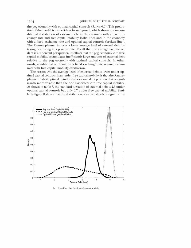
the peg economy with optimal capital controls (3.4 vs. 0.9). This predic-tion of the model is also evident from figure 8, which shows the uncon-ditional distribution of external debt in the economy with a fixed ex-change rate and free capital mobility (solid line) and in the economywith a fixed exchange rate and optimal capital controls (broken line).The Ramsey planner induces a lower average level of external debt bytaxing borrowing at a positive rate. Recall that the average tax rate ondebt is 2.4 percent per quarter. It follows that the peg economy with freecapital mobility accumulates inefficiently large amounts of external debtrelative to the peg economy with optimal capital controls. In otherwords, conditional on being on a fixed exchange rate regime, econo-mies with free capital mobility overborrow.The reason why the average level of external debt is lower under op-

timal capital controls than under free capital mobility is that the Ramseyplanner finds it optimal to induce an external debt position that is signif-icantly more volatile than the one associated with free capital mobility.As shown in table 3, the standard deviation of external debt is 2.3 underoptimal capital controls but only 0.7 under free capital mobility. Simi-larly, figure 8 shows that the distribution of external debt is significantly

FIG. 8.—The distribution of external debt


more dispersed under optimal capital controls than under free capitalmobility. A more volatile process for external debt requires centeringthe debt distribution further away from the natural debt limit for precau-tionary reasons. In turn, the reason why the Ramsey planner finds wideswings in the external debt position desirable is that such variations allowhim to insulate the domestic absorption of tradable goods from exoge-nous disturbances buffeting the economy. Put differently, in the Ramseyeconomy, external debt plays the role of shock absorber to a much largerextent than it does in the economy with free capital mobility.The purpose of optimal capital controls is not to close the current ac-

count. On the contrary, under optimal capital controls, the economymakes more heavy use of the current account to smooth consumptionthan it does under free capital mobility. To see this, note that the currentaccount is given by the change in net external debt and that, as is appar-ent from figure 8, the net external debt has a much more dispersed dis-tribution under optimal capital controls than under free capital mobility.Figure 8 shows that the distribution of net external debt under the op-

timal exchange rate policy (dotted line) has a higher mean and is muchless dispersed than under a currency peg with optimal capital controls.This difference highlights the fact that the two policies achieve reduc-tions in unemployment (relative to a currency peg with free capital mo-bility) through very different means. Under the optimal exchange ratepolicy, the government eliminates unemployment via devaluations thatshift the supply of nontradables to offset variations in the demand fornontradables brought about by fluctuations in the desired consumptionof tradables. In this way, the policy maker achieves two goals, full employ-ment and an efficient allocation of tradable consumption over time. Un-der a currency peg with optimal capital controls, the policy maker can-not induce shifts in the supply of nontradables, since its hands aretied by the currency peg and the presence of downward nominal wagerigidity. Instead, the government reduces unemployment by minimizingshifts in the demand for nontradables. To this end, the governmentlevies capital controls to stabilize the desired demand for tradable con-sumption, which is the key shifter of the demand schedule for non-tradables. In turn, as explained above, a smooth path for tradable con-sumption can be supported only by large swings in the country’sexternal debt position, which by necessity must be centered further awayfrom the natural debt limit than it would be if tradable consumptionwere allocated optimally.Finally, it is of interest to point out that the optimal capital control pol-

icy characterized here is complementary to the one that emerges inmodels of overborrowing due to collateral constraints (e.g., Korinek2010; Bianchi 2011). In this class of models, households’ ability to bor-row is increasing in the value of output in terms of tradables. In turn,


the value of output in terms of tradables is increasing in the relative priceof nontradables. This relative price is endogenous to the model but ex-ogenous to the household, which creates a pecuniary externality. Thegovernment understands that in equilibrium the relative price of non-tradables is increasing in the absorption of tradables. Consequently, toinduce a more relaxed collateral constraint on average, the governmentimplements a policy that raises the average consumption of tradedgoods. To support higher average consumption of tradables, the econ-omy must hold a lower average stock of external debt. This is achievedthrough capital controls. Thus, this literature shares two characteristicswith the present model, namely, an externality that leads to over-borrowing and positive average capital controls as a second-best remedy.The key difference, of course, resides in the nature of the externality, fi-nancial frictions in one case and downward wage rigidity in the other.

F. Welfare Costs of Free Capital Mobility under a Currency Peg

We have established that in the peg economy, free capital mobility en-tails excessive external debt and unemployment. Both of these factorstend to depress consumption and therefore reduce welfare. In this sec-tion, we quantify the welfare losses associated with free capital mobilityin economies subject to a currency peg.Define the welfare cost of a currency peg under free capital mobility

conditional on state st ; fyTt , rt , dt , wt21g, denoted lf ðstÞ, as the percent-age increase in the lifetime consumption stream required by an individ-ual living in the economy with a currency peg and free capital mobility instate st to be as well off as an individual living in an economy with the op-timal exchange rate policy. Formally, lf ðstÞ solves

E o∞

j50

bjU cft1j 1 1lf ðstÞ100

� �� st( )

5 voðyTt , rt , dtÞ,

where cft denotes consumption in the economy with a peg and free cap-ital mobility and, as defined earlier, voðyTt , rt , dtÞ denotes the value func-tion in the economy with the optimal exchange rate policy in stateðyTt , rt , dtÞ. Because the state vector st is stochastic, the conditional welfarecost measure, lf ðstÞ, is itself stochastic. We report the mean of lf ðstÞ overthe distribution of st in the peg economy with free capital mobility. For-mally, let pf ðstÞ denote the unconditional probability of st under a pegwith free capital mobility. Then

lf 5 ost

pf ðstÞlf ðstÞ: (35)


Similarly, the welfare cost of a currency peg under the optimal capitalcontrol policy conditional on state st, denoted lcðstÞ, is defined as thepermanent percentage increase in the lifetime consumption stream re-quired by an individual living in the economy with a currency peg andoptimal capital controls in state st to be as well off as an individual livingin the economy with the optimal exchange rate policy. That is, lcðstÞ isimplicitly given by

E o∞

j50

bjU cct1j 1 1lcðstÞ100

� �� st( )

5 voðyTt , rt , dtÞ,

where cct denotes consumption in the economy with a peg and optimalcapital controls. Letting pcðstÞ denote the unconditional probability ofst under a peg with optimal capital controls, we have that the expectedvalue of the welfare cost of a peg under the optimal capital control policyis given by

lc 5 ost

pcðstÞlcðstÞ: (36)

Recalling that the optimal exchange rate policy achieves the Pareto-optimal allocation, one can interpret lf as the distance, in welfare terms,between the first-best allocation and the allocation induced by a currencypeg with free capital mobility. Similarly, lc can be interpreted as the dis-tance between the first-best allocation and the one induced by a currencypeg coupled with Ramsey-optimal capital controls.Table 4 shows that the average welfare costs of free capital mobility for

a pegging economy are large. The representative household living in theeconomy with free capital mobility requires, on average, an increase of11.6 percent in consumption every period to be indifferent between liv-ing under a peg with free capital mobility and living in an economy withthe optimal exchange rate policy.The optimal capital control policy greatly reduces the pains of cur-

rency pegs. Households living in an economy with a currency peg and op-timal capital controls require a 3.7 percent increase in consumption eachperiod to be as well off as living in the economy with the optimal exchangerate policy. The welfare gain of moving from a peg, with or without opti-mal capital controls, to the optimal exchange rate policy has three compo-nents: One is a reduction in unemployment, which translates into higherproduction and consumption of nontradables. This benefit is larger forthe peg economy with free capital mobility. The second component is re-lated to transitional dynamics along which households liquidate precau-tionary savings through higher-than-average consumption of tradables.This effect can be seen from figure 8, showing that the average level of ex-ternal debt is higher under the optimal exchange rate policy than under


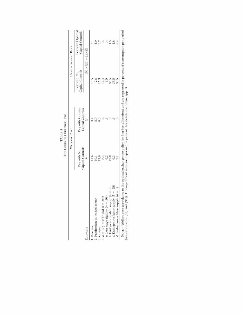
TABLE4

TheCostsofCurrencyPegs

WelfareCost

UnemploymentRate

Peg

withNo

Cap

ital

Controls

Peg

withOptimal

Cap

ital

Controls

Peg

withNo

Cap

ital

Controls

Peg

withOptimal

Cap

ital

Controls

Economy

lf

lc

100�

E½1

2ðh

t=� hÞ�

1.Baseline

11.6

3.7

13.5

3.1

2.Productionin

trad

edsector

10.1

5.0

7.8

1.9

3.Greece

17.6

6.0

15.3

3.7

4.j5

1/y5

2.27

andb5

.962

8.4

.612

.4.5

a.Lesswagerigidity(g

5.98)

6.2

.49.5

.4b.Endoge

nouslaborsupply(d

5.5)

19.0

.833

.51.3

c.Endoge

nouslaborsupply

(d5

.75)

9.3

.633

.51.8

d.Endoge

nouslaborsupply

(d5

1)2.1

.333

.58.4

Note.—

Welfare

costsarerelative

totheoptimalex

chan

gerate

policy

(orfirst-bestallocation)an

dareex

pressed

inpercentofco

nsumptionper

period

(see

expressions[35]

and[36]).Unem

ploym

entratesareex

pressed

inpercent.Fordetailsseeonlineap

p.G.

either of the two peg arrangements. The reduction in savings is greater forthe peg economy with optimal capital controls. The third component is alower long-run level of tradable consumption under the optimal ex-change rate policy. This component represents a cost and is higher un-der optimal capital controls than under free capital mobility. Overall, thewelfare gains are dominated by the reduction in unemployment.A relevant question from a policy perspective is what are the welfare

gains for a pegging economy with free capital mobility to adopt optimalcapital controls. One might be tempted to conclude that the answer islf 2 lc , or 7.9 percent of consumption per period. But this computationwould fail to correctly take into account the transitional debt dynamicsinvolved in moving from free capital mobility to optimal capital controls.As can be seen from figure 8, moving from a peg economy with free cap-ital mobility to a peg with optimal capital controls requires reducing theaverage level of external debt. This deleveraging is costly, since it im-plies a temporarily lower-than-average level of consumption of tradables.This sacrifice is painful by itself, but it also causes unemployment to behigher along the transition (recall that consumption of tradables is ashifter of the demand for nontradables). In the long run the economywith optimal capital controls will enjoy a higher average level of tradableconsumption than the economy with free capital mobility. In sum, mov-ing from free capital mobility to optimal capital controls has the benefitsof lower long-run unemployment (13.5 vs. 3.1 percent), higher long-runconsumption of tradables (6.9 percent higher), but a transitional cost as-sociated with debt deleveraging. Of course, by definition, there must benet gains from moving from free capital mobility to optimal capital con-trols. In our economy these gains turn out to be 2.2 percent of consump-tion per period.15 This is a large number as welfare costs go in businesscycle analysis but is not as high as the naive measure lf 2 lc .Our finding of large welfare costs of currency pegs (with or without

capital controls) stands in stark contrast to a large body of work, pio-neered by Lucas (1987), suggesting that the costs of business cycles(not just of suboptimal monetary policy) are small. Lucas’s approachto computing the welfare costs of business cycles abstracts from twofeatures that are central determinants of welfare costs in our model,

15 Formally, the welfare gain of switching from a peg with free capital mobility to a pegwith optimal capital controls, denoted lf → cðstÞ, is given by

lf → c 5 ost

pf ðstÞlf → cðstÞ,

where lf → cðstÞ is implicitly given by

E o∞

j50

bjU cft1j 1 1lf → cðstÞ100

� �� st( )

5 E o∞

j50

bjU ðcct1jÞ�� st

( ):


namely, the effect of volatility on mean unemployment and transitionaldynamics. The lack of connection between volatility and means withinLucas’s approach can be seen by noticing that it consists in first remov-ing a trend from a consumption time series and then evaluating asecond-order approximation of welfare using observed deviations ofconsumption from trend. Under this approach, the welfare cost of busi-ness cycles depends only on the volatility of the cyclical component ofconsumption. Implicit in this methodology is the assumption that thetrend is unaffected by policy. In our model, however, suboptimal mone-tary policy creates an endogenous connection between the amplitude ofthe business cycle and the average rate of unemployment. In turn,through its effect on the average level of unemployment, suboptimal ex-change rate policy has a significant effect on the average level of con-sumption of nontradables (recall that nontradables are produced withlabor). It follows that applying Lucas’s methodology to data stemmingfrom our model would overlook the effects of policy on mean consump-tion and therefore would result in spuriously low welfare costs.The importance of transitional dynamics for welfare can be seen by

comparing the mean and standard deviation of consumption in theeconomy with a peg and optimal capital controls and the economy withoptimal exchange rate policy. The welfare cost of pegs with optimalcapital controls relative to the optimal exchange rate policy is 3.7 per-cent of consumption per period even though consumption under theformer policy has a higher mean (0.97 vs. 0.93) and the same volatility(0.08) as under the latter. The reason why the peg with optimal capitalcontrols is welfare dominated by the economy with the optimal ex-change rate policy is that the former is associated with an inefficientlylow level of external debt. As a result, an economy that switches from apeg with optimal capital controls to the optimal exchange rate policyenjoys a transition with high absorption of tradables as it accumulatesexternal debt.Because our model is stylized, we interpret the present welfare evalu-

ation as suggestive. The sensitivity analysis presented in online appendixG and summarized in table 4 provides some more support for the size ofthe welfare losses reported here. In particular, it shows that the mainfindings are robust to allowing for production in the traded sector, esti-mating the driving process using data from Greece, considering a higherintertemporal elasticity of substitution (or lower value of j), allowing formore wage flexibility, and introducing endogenous labor supply.

X. Conclusion

We document the presence of downward nominal wage rigidity in low-inflation emerging economies with fixed nominal exchange rates. We


estimate that even in the context of massive unemployment, nominalhourly wages fail to fall at a rate larger than 1 percent per quarter. Withthis motivation in mind, we develop a dynamic stochastic model of anopen economy with downward nominal wage rigidity and analyze its ad-justment to large external shocks.A key insight of the model is that the combination of downward nom-

inal wage rigidity and a fixed exchange rate gives rise to a negative exter-nality. The nature of the externality is that private absorption expandstoo much in response to favorable shocks, causing inefficiently large in-creases in real wages. No problems are manifested in this phase of thecycle. However, as the economy falls back to its trend path, wages failto decline quickly enough because they are downwardly rigid. In addi-tion, the central bank, having its hands tied by the commitment to afixed exchange rate, cannot deflate the real value of wages via a devalu-ation. In turn, high real wages and a contracting level of aggregate ab-sorption cause involuntary unemployment. Individual agents are con-scious of this mechanism but are too small to internalize it. Theexternality thus leads to overborrowing during booms and to excessiveunemployment during downturns.We show that without policy intervention, currency pegs can be painful

for economies that are subject to large external shocks. For example, a cal-ibrated version of our model predicts that an external shock, defined as atwo standard deviation collapse in the terms of trade and a two standarddeviation increase in the country interest rate, causes an increase in unem-ployment of more than 20 percent of the labor force. This figure is consis-tent with the unemployment rates observed in the aftermath of recentlarge contractions in emerging-market economies that followed a fixed ex-change rate regime, including Argentina 1998–2001 and the periphery ofthe European Union after 2008.One policy option to address the unemployment problem is to abandon

the currency peg in favor of the optimal exchange rate policy.We show thatthe optimal exchange rate policy calls for large devaluations in response tolarge external shocks. These devaluations reduce the real value of wages,allowing the labor market to clear. In the calibrated model, boom-bust cy-cles of the typeobserved inArgentina in 1998–2001 and in the periphery ofEurope after 2008 call for devaluations of about 100 percent.We demonstrate that an alternative to devaluation is the optimal fiscal

policy. For example, optimal wage subsidies at the firm level financed byincome taxes at the household level can fully undo the distortions cre-ated by the combination of downward nominal wage rigidity and a cur-rency peg and therefore can bring about the Pareto-optimal allocation.We argue, however, that such policies might not be practical to imple-ment in a political environment focused on fiscal austerity such as theone prevailing in Europe after 2008. This motivates our analysis of opti-


mal capital control policy, broadly interpreted as regulations of cross-border financial flows, as an alternative way to address the aforemen-tioned negative externality.We show that the optimal capital control policy is prudential in nature.

The benevolent government taxes capital inflows in good times and sub-sidizes external borrowing in bad times. The key role of capital controlsis to insulate the domestic absorption of tradable goods from externalshocks. In this way, the government avoids that external disturbancesspill over to the nontraded sector causing unemployment. Capital con-trols, although they represent only a second-best policy, can go a longway toward restoring full employment in fixed exchange rate economies.Under our baseline calibration, the average rate of unemployment fallsfrom 13.5 to 3.1 percent when the currency peg is coupled with optimalcapital controls.These results suggest that when labor markets suffer from downward

nominal wage rigidity and the exchange rate is fixed, countercyclicalcapital controls can be an effective instrument for macroeconomic sta-bilization.

References

Akinci, Özge. 2011. “A Note on the Estimation of the Atemporal Elasticity ofSubstitution between Tradable and Nontradable Goods.” Manuscript (Febru-ary 2), Columbia Univ.

Auernheimer, L., and R. García-Saltos. 2000. “International Debt and the Priceof Domestic Assets.”Working Paper no. wp/00/177 (October), Internat. Mon-etary Fund, Washington, DC.

Barattieri, Alessandro, Susanto Basu, and Peter Gottschalk. 2010. “Some Evi-dence on the Importance of Sticky Wages.” Working Paper no. 16130 ( June),NBER, Cambridge, MA.

Barkbu, Bergljot, Jesmin Rahman, and Rodrigo Valdés. 2012. “Fostering Growthin Europe Now.” Staff Discussion Note no. SDN-12-07 ( June 18), Internat. Mon-etary Fund, Washington, DC.

Benigno, Gianluca, Huigang Chen, Christopher Otrok, Alessandro Rebucci,and Eric R. Young. 2011. “Revisiting Overborrowing and Its Policy Implica-tions.” In Monetary Policy under Financial Turbulence, edited by Luis FelipeCespedes, Roberto Chang, and Diego Saravia, 145–84. Santiago: CentralBank Chile.

Bianchi, Javier. 2011. “Overborrowing and Systemic Externalities in the BusinessCycle.” A.E.R. 101 (December): 3400–3426.

Bianchi, Javier, and Enrique G. Mendoza. 2012. “Overborrowing, Financial Cri-ses and Macroprudential Policy.” Manuscript ( July), Univ. Wisconsin.

Blundell, Richard, and Thomas MaCurdy. 1999. “Labor Supply: A Review of Al-ternative Approaches.” In Handbook of Labor Economics, vol. 3, edited by OrleyAshenfelter and David Card, 1559–1695. Amsterdam: North-Holland.

Caballero, Ricardo J., and Guido Lorenzoni. 2009. “Persistent Appreciations andOvershooting: A Normative Analysis.” Manuscript (February), MassachusettsInst. Tech.


Costinot, Arnaud, Guido Lorenzoni, and Iván Werning. 2011. “ATheory of Cap-ital Controls as Dynamic Terms-of-Trade Manipulation.” Working Paper no.17680 (December), NBER, Cambridge, MA.

Daly, Mary, Bart Hobijn, and Brian Lucking. 2012. “Why Has Wage GrowthStayed Strong?” Fed. Reserve Bank San Francisco Econ. Letter 2012-10 (April 2).

Eichengreen, Barry, and Jeffrey Sachs. 1985. “Exchange Rates and Economic Re-covery in the 1930s.” J. Econ. Hist. 45 (December): 925–46.

Elsby, Michael. 2009. “Evaluating the Economic Significance of Downward Nom-inal Wage Rigidity.” J. Monetary Econ. 56 (March): 154–69.

Erceg, Christopher J., Dale W. Henderson, and Andrew T. Levin. 2000. “OptimalMonetary Policy with Staggered Wage and Price Contracts.” J. Monetary Econ.46:281–314.

Farhi, Emmanuel, G. Gopinath, and O. Itskhoki. 2011. “Fiscal Devaluations.”Manuscript, Harvard Univ.

Farhi, Emmanuel, and Iván Werning. 2012. “Dealing with the Trilemma: Opti-mal Capital Controls with Fixed Exchange Rates.” Working Paper no. 18199( June), NBER, Cambridge, MA.

Fehr, Ernst, and Lorenz Goette. 2005. “Robustness and Real Consequences ofNominal Wage Rigidity.” J. Monetary Econ. 52 (May): 779–804.

Fortin, Pierre. 1996. “The Great Canadian Slump.” Canadian J. Econ. 29 (Novem-ber): 761–87.

Galí, Jordi. 2011. Unemployment Fluctuations and Stabilization Policies: A New Keynes-ian Perspective. Cambridge, MA: MIT Press.

Galí, Jordi, and Tommaso Monacelli. 2005. “Monetary Policy and Exchange RateVolatility in a Small Open Economy.” Rev. Econ. Studies 72 ( July): 707–34.

García-Cicco, Javier, Roberto Pancrazi, and Martín Uribe. 2010. “Real BusinessCycles in Emerging Countries?” A.E.R. 100:2510–31.

González Rozada, Martín, Pablo Andrés Neumeyer, Alejandra Clemente, DiegoLuciano Sasson, and Nicholas Trachter. 2004. “The Elasticity of Substitution inDemand for Non-tradable Goods in Latin America: The Case of Argentina.”Research Network Working Paper no. R-485 (August), Inter-American Devel-opment Bank, Washington, DC.

Gottschalk, Peter. 2005. “Downward Nominal-Wage Flexibility: Real or Measure-ment Error?” Rev. Econ. and Statis. 87 (August): 556–68.

Holden, Steinar, and Fredrik Wulfsberg. 2008. “Downward Nominal Wage Rigid-ity in the OECD.” B.E. J. Macroeconomics 8:art. 15.

Jeanne, Olivier, and Anton Korinek. 2013. “Macroprudential Regulation versusMoppingUp after the Crash.”Working Paper no. 18675 ( January), NBER, Cam-bridge, MA.

Justiniano, Alejandro, Giorgio Primiceri, and Andrea Tambalotti. 2010. “Invest-ment Shocks and Business Cycles.” J. Monetary Econ. 57 (March): 132–45.

Kaur, Supreet. 2012. “Nominal Wage Rigidity in Village Labor Markets.” Manu-script ( January), Harvard Univ.

Kollmann, Robert. 2002. “Monetary Policy Rules in the Open Economy: Effectson Welfare and Business Cycles.” J. Monetary Econ. 49 ( July): 989–1015.

Korinek, Anton. 2010. “Excessive Dollar Borrowing in Emerging Markets: BalanceSheet Effects and Macroeconomic Externalities.” Manuscript, Univ. Maryland.

Kuroda, Sachiko, and Isamu Yamamoto. 2003. “Are Japanese Nominal WagesDownwardly Rigid? Part I: Examinations of Nominal Wage Change Distribu-tions.” Monetary and Econ. Studies, Bank of Japan 21 (August): 1–29.

Lane, Philip R., and Gian Maria Milesi-Ferretti. 2007. “The External Wealth ofNations Mark II: Revised and Extended Estimates of Foreign Assets and Liabil-ities, 1970–2004.” J. Internat. Econ. 73 (November): 223–50.


Lorenzoni, Guido. 2008. “Inefficient Credit Booms.” Rev. Econ. Studies 75:809–33.

Lucas, Robert E., Jr. 1987. Models of Business Cycles. Cambridge, MA: Blackwell.Obstfeld, Maurice, and Kenneth Rogoff. 1996. Foundations of International Macro-

economics. Cambridge, MA: MIT Press.Reinhart, Carmen M., and Carlos A. Végh. 1995. “Nominal Interest Rates, Con-

sumption Booms, and Lack of Credibility: A Quantitative Examination.” J. De-velopment Econ. 46 (April): 357–78.

Schmitt-Grohé, Stephanie, and Martín Uribe. 2003. “Closing Small Open Econ-omy Models.” J. Internat. Econ. 61 (October): 163–85.

———. 2009. “Finite-State Approximation of VAR Processes: A Simulation Ap-proach.” Manuscript, Columbia Univ.

———. 2010. “Pegs and Pain.” Manuscript, Columbia Univ.———. 2012. “Prudential Policy for Peggers.” Manuscript, Columbia Univ.Smets, Frank, and Raf Wouters. 2007. “Shocks and Frictions in US Business

Cycles: A Bayesian DSGE Approach.” A.E.R. 97 ( June): 586–606.Stockman, Alan C., and Linda L. Tesar. 1995. “Tastes and Technology in a Two-

Country Model of the Business Cycle: Explaining International Comove-ments.” A.E.R. 85 (March): 168–85.

Uribe, Martín. 1997. “Exchange-Rate-Based Inflation Stabilization: The InitialReal Effects of Credible Plans.” J. Monetary Econ. 39 ( June): 197–221.

———. 2006. “On Overborrowing.” A.E.R. Papers and Proc. 96 (May): 417–21.———. 2007. “Individual versus Aggregate Collateral Constraints and the Over-

borrowing Syndrome.”Working Paper no. 12260 (May),NBER,Cambridge,MA.


Downward Nominal Wage Rigidity, Currency Pegs, and ...mu2166/dnwr_pegs_iu/paper.pdf · Downward...

Documents

Transcript of Downward Nominal Wage Rigidity, Currency Pegs, and ...mu2166/dnwr_pegs_iu/paper.pdf · Downward...