Prêmio Banco Central de Economia e FinançasPolítica Monetária • 3º lugar

Asymmetric Price and Wage Rigidity in Brazil: Estimation of a DSGE Model via Particle Filter

Ederson Luiz Schumanski

ederson_schumanski@sicredi.com.brmrrede@hotmail.com

Brasília • 2015

1

Asymmetric Price and Wage Rigidity in Brazil:

Estimation of a DSGE Model via Particle Filter

Abstract

The aim of this paper is to check whether price and wage rigidity are asymmetric in

the Brazilian economy, i.e., whether economic agents adjust them downward or upward. In

addition, the effects of monetary and fiscal policies on the dynamics of the economy are

assessed. To do that, a nonlinear dynamic stochastic general equilibrium (DSGE) model with

asymmetry in price and wage adjustment costs is used, following Aruoba, Bocola, and

Schorfheide (2013). This model can produce downward (or upward) price or wage rigidity,

which could give rise to strong nonlinearities. Therefore, the model is solved using a

nonlinear method and its parameters are estimated by a particle filter. Results indicate that

both nominal prices and wages are stickier downward and asymmetric rigidity has an impact

on the dynamics of the economy whenever monetary and fiscal policy shocks are present. If

the Central Bank implements the monetary policy without considering the effects of

asymmetric rigidity, the policy will be suboptimal.

Keywords: DSGE. Particle filter. Monetary and fiscal policy. Nonlinear solution method.

Asymmetric adjustment costs.

JEL codes: C11, C15, E52, E62

2

1. Introduction

The so-called Lucas (1976) critique was a milestone in the improvement of modeling

and analysis of macroeconomic models in the 1970s. The assessment of economic policies

through econometric models might be detrimental as the parameters of these models are not

structural, i.e., they are not invariant to policy regime shifts. In other words, the relationships

between aggregate variables would tend to change whenever macroeconomic policies were

altered. Thus, in response to the Lucas critique, several macroeconomic models were built

upon microfoundations (DSGE).

In the past 20 years, huge improvements have been made in macroeconomic modeling

and DSGE models have gained momentum both among scholars and economists. Many

central banks around the globe have developed their own DSGE models to assess economic

policies and macro variables movements. Given the growing importance of these models for

quantitative analyses, their estimation has become increasingly popular. The usual method to

estimate the structural parameters of these models consists of Bayesian techniques and

likelihood-based inference in order to take the information from the dataset to the model

economy, as pointed out by An & Schorfheide (2007). First, the DSGE model is submitted to

some solution method and represented in state space and, then, filtering methods are used to

estimate likelihood. However, most dynamic models do not have a likelihood function that

can be calculated analytically or numerically.

As a way to circumvent this problem, most papers on dynamic economies focus on

log-linearized equilibrium conditions, eventually turning the Kalman filter into an essential

tool for the simulation of unobservable variables and for the estimation of likelihood of

models that describe the behavior of the economy of interest, allowing parameters to be

estimated by Bayesian techniques. Nonetheless, the Kalman filter is somewhat restrictive –

3

with linear state-space representation and Gaussian perturbations – thus limiting the analysis

of nonlinear phenomena likely to be observed in the data. Fasolo (2012) mentions some

examples of nonlinearities usually observed in the data: the influence of risk aversion and of

precautionary saving on aggregate variables, such as consumption and investment; the so-

called “fat-tails” often seen in economic shocks and fiscal and monetary policy regime shifts;1

all of which cannot be properly described by a linear model. Although the economics

literature has not reached a consensus about the advantages of the estimation of nonlinear

approximations in DSGE models, Fernández-Villaverde, Rubio-Ramírez & Santos (2006)

theoretically demonstrate that nonlinear approximations in the DSGE model investigated by

them led to a more accurate estimation of the “peak” of the likelihood function, which would

consequently have some impact on the estimation of structural parameters of the economy at

issue. The authors point out that second-order errors in policy functions cause first-order

errors in the likelihood function that arises from the process, which could consequently

produce disastrous results for linear estimators, as first-order errors in the likelihood function

yield biased parameter estimates. Moreover, the authors show that errors in the approximate

likelihood function would build up with the increase in sample size. In other words, the

approximation errors associated with the linear representation of DSGE models may lead to

significant errors in the corresponding likelihood functions2 and, therefore, as a result, the

approximation of likelihood functions based on a model solved via a linear solution method,

may differ from an exact likelihood estimation.

1There are two examples of a monetary policy regime shift in the Brazilian economy: the first one refers to when

Gustavo Franco, the then-president of the Central Bank of Brazil, was replaced with Armínio Fraga in 1999, who

took over and had his mind set on adopting the inflation-targeting regime, which he eventually did in July 1999,

under Resolution 2.615, issued by the National Monetary Council (Giambiagi & Villela, 2005). The second case

was when Alexandre Tombini – the current president of the Central Bank – replaced Henrique Meirelles in 2011,

adopting a more tolerant stance on inflation, reducing the Selic rate to its historical minimum of 7.25 pp and

keeping it at low levels even when inflation is above the midpoint of the target range (4.5%). 2 Alves (2011) performs a simulation using a comprehensive set of artificial data based on a nonlinear solution of

a DSGE model and estimates the structural parameters via log-linear approximations around steady state

conditions. The author finds a significant bias in Calvo (1983) stickiness parameter estimates – price rigidity and elasticity of labor supply.

4

By taking these problems into account and attempting to solve them, Fernández-

Villaverde & Rubio-Ramírez (2005) propose the use of a particle filter to estimate the

likelihood of the neoclassical growth model and gather empirical evidence about the

superiority of nonlinear DSGE estimators to linear ones. However, the empirical evidence

provided by the authors cannot be generalized, as it is valid only for the simple model used.

Therefore, to put forward stronger arguments in favor of nonlinear methods, Villaverde &

Rubio-Ramírez (2007) estimate an extended version of the neoclassical growth model and add

essential nonlinearities using the argument that the shocks that underlie the model are subject

to stochastic volatility, and thus linear approximations would eventually cancel out the effects

of these shocks, rendering this type of approximation inefficient, consequently making

nonlinear approximations grow in popularity.

Accordingly, the use of likelihood-based inference becomes important for some

reasons. First, following Monfort (1996), from an empirical perspective, this type of inference

is a simple way to deal with misspecified models, which is the case of dynamic steady-state

economies, which are false by construction, making likelihood-based inference attractive due

to its asymptotic properties and to its good behavior in small samples, even when models are

misspecified, as argued by Fernández-Villaverde & Rubio-Ramírez (2005). From a theoretical

viewpoint, it is assumed that any empirical evidence obtained from data should be included in

the likelihood function, as highlighted by Berger & Wolpert (1988). Given this background

information, it seems plausible to say that the closer researchers get to the likelihood of the

analyzed model, that is, the closer they get to the actual likelihood, the more they will be able

to extract all the necessary and available information from the data. Therefore, the appropriate

selection of the approximation method is crucial to researchers, as this will enormously

influence the likelihood function of the model to be studied.

5

First of all, after having a look at the previous arguments, the selection of a nonlinear

approximation method seems to be highly recommendable to solve a dynamic steady-state

model. Notwithstanding, one should bear in mind that models which do not include some kind

of nonlinearity and are submitted to nonlinear approximation methods are conducive to a

steady state that is quite similar to the that found in linear estimations. Hence, the use of

nonlinear solution methods is only useful when the model presents some kind of

nonlinearity.3 In the present paper, the use of nonlinear solution methods is necessary because

of the model used. The focus is on the estimation of a new Keynesian model with asymmetric

price and wage adjustment costs, following Kim & Ruge-Murcia (2009) and Aruoba, Bocola

& Shorfheide (2013). This model can produce downward (or upward) price and wage rigidity.

By allowing asymmetry in adjustment costs, the economic agents’ decision-making rules may

become strongly nonlinear. The key feature of the model is the introduction of asymmetry in

price and wage adjustment costs. In other words, besides taking into account price and wage

rigidity, the model also adds asymmetry in rigidity. So, depending on the sign and size of the

parameters associated with asymmetry, prices and wages in the Brazilian economy can be

stickier downward or upward. These asymmetries may be caused by the Brazilian labor

market framework, due to the high percentage of informal jobs and turnover, as well as to the

large number of military jobs and civil servants, among whom wages are stickier. Moreover,

these asymmetries may influence prices at the firm level, since most of the costs Brazilian

firms have to cover are associated with the payment of their employees’ wages; in addition,

3 According to Aruoba, Bocola & Shorfheide (2013), there are two types of nonlinearities that may be seen in

nonlinear DSGE models. The first ones are known as approximately smooth nonlinearities, in which decision

rules contain slopes and, possibly, asymmetries as those which are generated by cost functions or asymmetric

loss functions. The other type refers to “kinks” in decision rules, such as those generated by the zero lower

bound in nominal interest rates. Also, the authors mention that nonlinear characteristics may be endogenous or

exogenous. Slopes in utility functions, in adjustment cost functions, and in production functions may

endogenously give rise to nonlinear decision rules households and firms abide by. On the other hand, an example

of an exogenous linearity is the stochastic volatility to which exogenous shocks are subjected, which causes business cycle movements.

6

(downward or upward) rigidity is also expected to influence the prices of goods, which may

be even stickier (either upward or downward) than wages, thereby causing more harmful

inflationary effects on the economy as a whole. Thus, in a more rigid economy where prices

and wages are cut, expansionary monetary policy shocks, by means of a decrease in interests

or of fiscal shocks, such as tax reduction or increase in government spending, could force the

economy into longer periods of high inflation, bringing about economic imbalance, which

would take longer to be overcome.

All that being said, the present paper seeks to answer the following questions: is price

and wage rigidity in the Brazilian economy asymmetric, i.e., do economic agents act

nonlinearly, being more reluctant to adjust prices and wages downward instead of upward? If

so, how do these asymmetries eventually influence economic behavior when the economy

faces a temporary monetary and fiscal policy shock? So, the present paper aims to estimate

the structural parameters of Brazilian economy – especially those which have to do with

asymmetric rigidity - and to assess the behavior of the major macroeconomic variables

towards monetary and fiscal policy movements. A DSGE model, proposed by Kim & Ruge-

Murcia (2009) and extended by Aruoba, Bocola & Shorfheide (2013), is then used with

asymmetric price and wage adjustment costs, which could lead to nonlinearities in economic

agents’ behaviors. The model is solved using perturbation methods and is estimated with

Brazilian data via a particle filter, in order to construct the likelihood. It is important to stress

that the particle filter can be used to estimate models other than the nonlinear ones.

Empirically, it proved to be superior to the Kalman filter in DSGE models. Several authors

reported superior performance of their estimates made from the nonlinear model estimated by

sequential Monte Carlo methods. Among these authors are An & Schorfheide (2007),

Fernández-Villaverde & Rubio-Ramírez (2007) and Amisano & Tristani (2010), who

compare their findings using a model solved by a nonlinear method, and hence estimated by a

7

particle filter, and the same model in linearized form estimated by the Kalman filter. Even in

the work of Fernández-Villaverde & Rubio-Ramírez (2005), in which the authors estimate a

quasilinear model (neoclassical growth model), the particle filter outperformed the Kalman

filter.

The paper is organized into four sections, in addition to the introduction. Section 2

introduces the nonlinear DSGE model with asymmetric price and wage adjustment costs and

provides a brief analysis of the solution method used. Section 3 describes the estimation

method, which focuses on the particle filter. Section 4 presents and comments on the results

of the empirical analysis. Section 5 concludes.

2. The Theoretical Model

2.1. Evolution of DSGE Models and the New Keynesian Approach

The attempt to understand and analyze how fluctuations occur in macroeconomic

variables – such as output, inflation, unemployment, among others – prompted many

economic researchers to develop several models, from the mid-20th century onwards, to

explain these phenomena. Improvements in macroeconomic theory, along with the

development of econometric techniques, allowed constructing more robust models based on

microeconomic foundations, with good performance in the adjustment of data and forecasts.

These models are known as DSGE (dynamic stochastic general equilibrium). “Dynamic”

because time matters, i.e., the past influences the present, and the future (through

expectations) also influences the present. “Stochastic” because there are structural shocks,

which are accountable for cycles and fluctuations in several macroeconomic variables. And

finally, “General Equilibrium” because funds in the economy are allocated via markets, i.e.,

there are several interdependent markets that interact with each other in a given time period.

8

Kydland & Prescott (1982) provided the necessary tools to assess the behavior of

economic movements. These authors built a model assuming a perfectly competitive market

where utility maximizing agents would be subject to budget and technological constraints.

According to Romer (2012), what these real business cycle models seek is the construction of

a microfounded general equilibrium model and the specification of the shocks observed in the

main macroeconomic movements. In addition, according to Rebelo (2005), there were three

revolutionary ideas in the seminal work published in 1982. The first one, based on the

previous work of Lucas & Prescott (1971), claims that business cycles can be analyzed by

dynamic general equilibrium models. The second one shows the possibility to combine

business cycles with the growth theory, highlighting that business cycles must be consistent

with empirical regularities in long-term growth. Finally, the third idea proposes going way

beyond the qualitative comparison of the model’s properties with stylized facts that were

predominant in theoretical studies until 1982.

The main advantage of the real business cycle model is that it is not subject to Sims4

and Lucas5 critiques, as these models are hinged upon microeconomic foundations. In other

words, the restrictions imposed on the variables would not occur on an ad hoc basis, since

they would be based on the description of behaviors of consumers, firms, and government.

Furthermore, the parameters of these models are deemed to be structural, as they remain

unchanged when faced with monetary policy regime shifts since they are closely related to

preferences and technology, which tend to be stable in the short and medium run. On the other

hand, the downside of the model is that it is not checked in practice due to the lack of a

4 Sims (1980) argues that the restrictions imposed on structured models aimed at making them identifiable were

too strong and then undermined the efficiency and quality of forecasts. The author introduced the vector

autoregressive (VAR) model, which was not theoretical and did not require that structured models be

identifiable. 5 Lucas (1976) argues that the use of econometric models aimed at the formulation of economic policies could be

harmful, as the parameters of these models would not be structural; i.e., they would not be invariant to the

economic policy and would thus be susceptible to variations whenever changes occurred in the economic scenario.

9

monetary sector. This sector is not necessary because the presence of perfect competition and

totally flexible prices render money superneutral, not affecting real economic variables, i.e.,

the monetary policy in this type of model is irrelevant. However, in empirical studies as those

of Christiano, Eichenbaum & Evans (1999), superneutrality was not observed in real data,

prompting criticisms against real business cycles for their lack of empirical evidence.

Owing to the harsh criticisms against real business cycles regarding empirical

evidence that the forecasts made by the model about monetary disturbances were unrealistic,

some assumptions had to be reconsidered. According to Galí (2008), departing from the real

business cycle, the change in some assumptions about the original model and the introduction

of some frictions gave rise to the new Keynesian model, which contemplates a monopolistic

competition across firms and the introduction of nominal rigidity – implying nonneutrality of

money in the short run. Most of current DSGE models assume that prices and/or wages are

sticky in nominal terms, i.e., they are not adjusted perfectly in each period. The two pricing

mechanisms most widely used in the macroeconomic literature are those by Calvo (1983) and

by Rotemberg (1982). The former one assumes that prices are gradually adjusted at random

intervals and that this sort of rigidity is investigated in studies like those of Christiano,

Eichenbaum & Evans (2005) and Smets & Wouters (2004). In the latter mechanism, proposed

by Rotemberg, prices are adjusted more slowly than what would be ideal, but identically by

all firms, implying convex costs. This type of rigidity was used by Schmitt-Grohé & Uribe

(2004) and by An & Schorfheide (2007).

2.2. DSGE Model with Asymmetric Price and Wage Adjustment Costs

The model dealt with herein consists of a single final good firm and of a continuum of

intermediate good producing firms used as input for the former. Moreover, a representative

household that maximizes its intertemporal utility, subject to budget constraint, is included.

10

Finally, in the last economic sector, there is a monetary and fiscal authority. The model is

based on Kim & Ruge-Murcia (2009) and Aruoba, Bocola & Shorfheide (2013), in which the

authors replace the adjustment cost functions proposed by Rotemberg (1982) with “linex”

adjustment cost functions, which can capture downward (or upward) price and wage rigidity.

The model leaves capital accumulation aside and deals with a closed economy, for the sake of

simplicity. In the present paper, the aim of using these asymmetric adjustment cost functions

is to try to describe the behavior of price setters in a more realistic fashion, thus seeking to

elucidate wage and price movements. Apparently, both methods proposed by Calvo (1983)

and Rotemberg (1982) to produce wage and price rigidity do not lead to a complete rigidity

mechanism. These methods regard rigidity as symmetrical, i.e., they do not take into

consideration that economic agents might cause prices to be stickier downward than upward,

resulting in asymmetric rigidity. In other words, it seems plausible to believe that employers

are much stricter about reducing wages than about raising them; additionally, in the case of

firms, they are stricter about reducing the prices of their goods than about increasing them,

especially in a monopolistically competitive market, where firms exercise some monopoly.

The use of these functions is also justified by the empirical evidence that their introduction

produce nonlinearities in the DSGE model that can explain the nonlinearities observed in U.S.

data, as shown by Aruoba, Bocola & Shorfheide (2013). Nevertheless, the authors underscore

that the nonlinear dynamics observed in inflation and in wages do not produce nonlinearities

in GDP growth or in the interest rate. So, the nonlinearities seen in the dynamics of wages and

prices do not spread explicitly across the other U.S. economic variables. The equations for the

model proposed by Aruoba, Bocola & Shorfheide (2013) are presented in what follows.

11

2.2.1 Firms

In the proposed model, a country produces a single final good and a set of intermediate

goods indexed by 𝑗 ∈ [0,1]. The firms that manufacture final goods are perfectly competitive

and the good is consumed by households. In their turn, intermediate good firms manufacture

differentiated goods in a monopolistically competitive market.

Final good firms are perfectly competitive and combine intermediate goods indexed

by 𝑗 ∈ [0,1] using the following production function:

𝑌𝑡 = (∫ 𝑌𝑡(𝑗)1−𝜆𝑝,𝑡𝑑𝑗1

0)

1

1−𝜆𝑝,𝑡. (1)

Note that 1 𝜆𝑝,𝑡 > 1⁄ represents elasticity of demand for each intermediate good that

embodies the technology. Given that final good firms are in a perfectly competitive market,

they maximize their profits according to production function (1) using the prices of all

intermediate goods 𝑃𝑡(𝑗) and the price of final goods 𝑃𝑡. The maximization problem is then

expressed as:

𝑚𝑎𝑥𝑌𝑡(𝑗)𝑃𝑡𝑌𝑡 − ∫ 𝑃𝑡(𝑗)𝑌𝑡(𝑗)1

0𝑑𝑗. (2)

By solving the firm’s problem, one obtains the input demand function, which is given by:

𝑌𝑡(𝑗) = (𝑃𝑡(𝑗)

𝑃𝑡)

−1𝜆𝑝,𝑡

⁄𝑌𝑡. (3)

In equation (3), the demand for intermediate goods depends on price 𝑃𝑡 (𝑗) of the intermediate

good relative to price 𝑃𝑡 of the final good. By using aggregate demand 𝑌𝑡 together with the

12

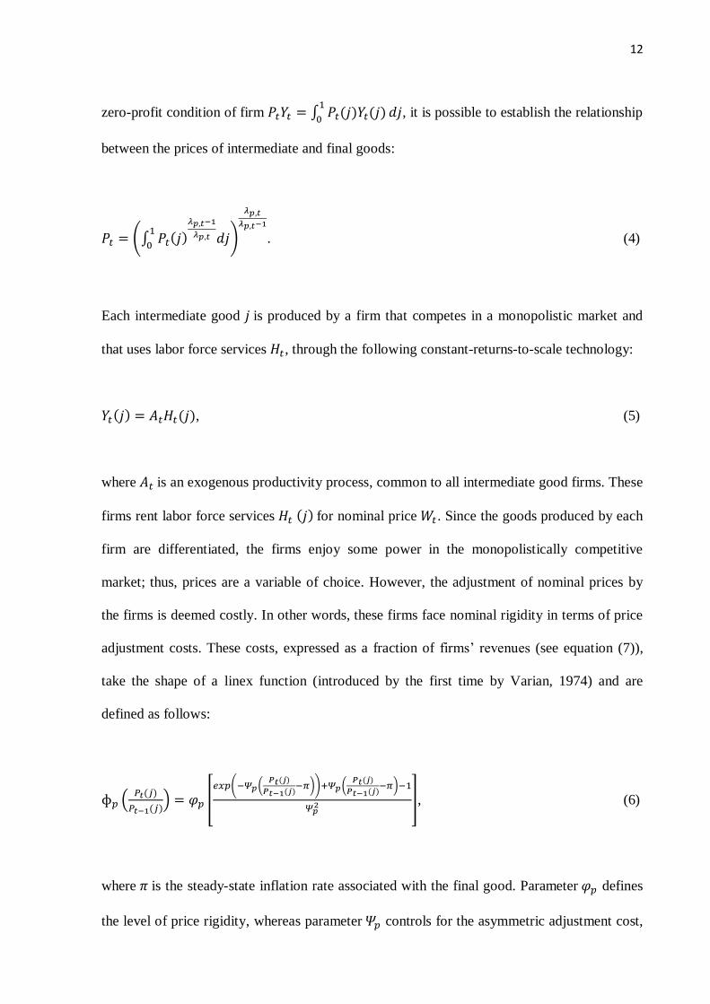
zero-profit condition of firm 𝑃𝑡𝑌𝑡 = ∫ 𝑃𝑡(𝑗)𝑌𝑡(𝑗)1

0𝑑𝑗, it is possible to establish the relationship

between the prices of intermediate and final goods:

𝑃𝑡 = (∫ 𝑃𝑡(𝑗)𝜆𝑝,𝑡−1

𝜆𝑝,𝑡 𝑑𝑗1

0)

𝜆𝑝,𝑡

𝜆𝑝,𝑡−1

. (4)

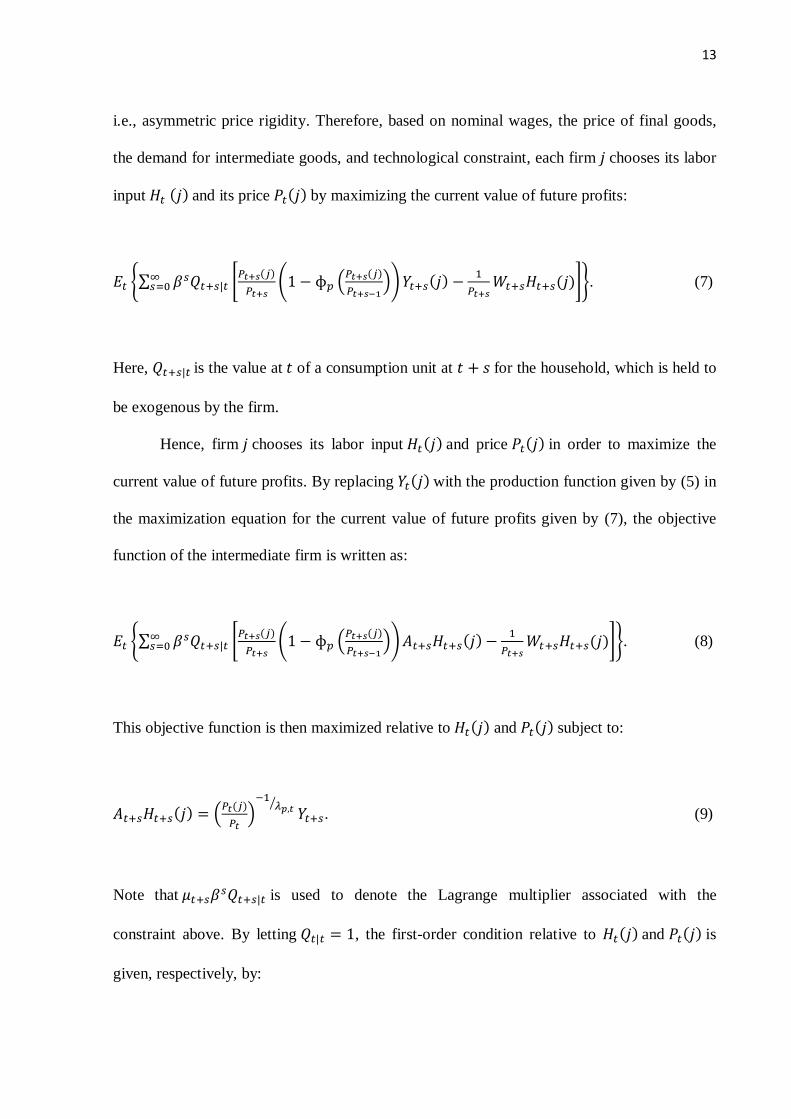
Each intermediate good 𝑗 is produced by a firm that competes in a monopolistic market and

that uses labor force services 𝐻𝑡, through the following constant-returns-to-scale technology:

𝑌𝑡(𝑗) = 𝐴𝑡𝐻𝑡(𝑗), (5)

where 𝐴𝑡 is an exogenous productivity process, common to all intermediate good firms. These

firms rent labor force services 𝐻𝑡 (𝑗) for nominal price 𝑊𝑡. Since the goods produced by each

firm are differentiated, the firms enjoy some power in the monopolistically competitive

market; thus, prices are a variable of choice. However, the adjustment of nominal prices by

the firms is deemed costly. In other words, these firms face nominal rigidity in terms of price

adjustment costs. These costs, expressed as a fraction of firms’ revenues (see equation (7)),

take the shape of a linex function (introduced by the first time by Varian, 1974) and are

defined as follows:

ɸ𝑝 (𝑃𝑡(𝑗)

𝑃𝑡−1(𝑗)) = 𝜑𝑝 [

𝑒𝑥𝑝(−𝛹𝑝(𝑃𝑡(𝑗)

𝑃𝑡−1(𝑗)−𝜋))+𝛹𝑝(

𝑃𝑡(𝑗)

𝑃𝑡−1(𝑗)−𝜋)−1

𝛹𝑝2 ], (6)

where 𝜋 is the steady-state inflation rate associated with the final good. Parameter 𝜑𝑝 defines

the level of price rigidity, whereas parameter 𝛹𝑝 controls for the asymmetric adjustment cost,

13

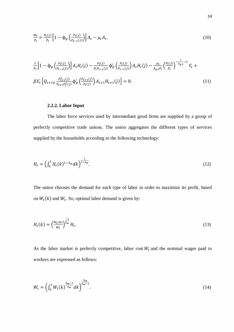
i.e., asymmetric price rigidity. Therefore, based on nominal wages, the price of final goods,

the demand for intermediate goods, and technological constraint, each firm 𝑗 chooses its labor

input 𝐻𝑡 (𝑗) and its price 𝑃𝑡(𝑗) by maximizing the current value of future profits:

𝐸𝑡 {∑ 𝛽𝑠𝑄𝑡+𝑠|𝑡 [𝑃𝑡+𝑠(𝑗)

𝑃𝑡+𝑠(1 − ɸ𝑝 (

𝑃𝑡+𝑠(𝑗)

𝑃𝑡+𝑠−1)) 𝑌𝑡+𝑠(𝑗) −

1

𝑃𝑡+𝑠𝑊𝑡+𝑠𝐻𝑡+𝑠(𝑗)]∞

𝑠=0 }. (7)

Here, 𝑄𝑡+𝑠|𝑡 is the value at 𝑡 of a consumption unit at 𝑡 + 𝑠 for the household, which is held to

be exogenous by the firm.

Hence, firm 𝑗 chooses its labor input 𝐻𝑡(𝑗) and price 𝑃𝑡(𝑗) in order to maximize the

current value of future profits. By replacing 𝑌𝑡(𝑗) with the production function given by (5) in

the maximization equation for the current value of future profits given by (7), the objective

function of the intermediate firm is written as:

𝐸𝑡 {∑ 𝛽𝑠𝑄𝑡+𝑠|𝑡 [𝑃𝑡+𝑠(𝑗)

𝑃𝑡+𝑠(1 − ɸ𝑝 (

𝑃𝑡+𝑠(𝑗)

𝑃𝑡+𝑠−1)) 𝐴𝑡+𝑠𝐻𝑡+𝑠(𝑗) −

1

𝑃𝑡+𝑠𝑊𝑡+𝑠𝐻𝑡+𝑠(𝑗)]∞

𝑠=0 }. (8)

This objective function is then maximized relative to 𝐻𝑡(𝑗) and 𝑃𝑡(𝑗) subject to:

𝐴𝑡+𝑠𝐻𝑡+𝑠(𝑗) = (𝑃𝑡(𝑗)

𝑃𝑡)

−1𝜆𝑝,𝑡

⁄𝑌𝑡+𝑠. (9)

Note that 𝜇𝑡+𝑠𝛽𝑠𝑄𝑡+𝑠|𝑡 is used to denote the Lagrange multiplier associated with the

constraint above. By letting 𝑄𝑡|𝑡 = 1, the first-order condition relative to 𝐻𝑡(𝑗) and 𝑃𝑡(𝑗) is

given, respectively, by:

14

𝑊𝑡

𝑃𝑡=

𝑃𝑡(𝑗)

𝑃𝑡[1 − ɸ𝑝 (

𝑃𝑡(𝑗)

𝑃𝑡−1(𝑗))] 𝐴𝑡 − 𝜇𝑡𝐴𝑡. (10)

1

𝑃𝑡[1 − ɸ𝑝 (

𝑃𝑡(𝑗)

𝑃𝑡−1(𝑗))] 𝐴𝑡𝐻𝑡(𝑗) −

𝑃𝑡(𝑗)

𝑃𝑡𝑃𝑡−1(𝑗)ɸ𝑝

′ (𝑃𝑡(𝑗)

𝑃𝑡−1(𝑗)) 𝐴𝑡𝐻𝑡(𝑗) −

𝜇𝑡

𝜆𝑝,𝑡𝑃𝑡(

𝑃𝑡(𝑗)

𝑃𝑡)

−1

𝜆𝑝,𝑡−1

𝑌𝑡 +

𝛽𝐸𝑡 {𝑄𝑡+1|𝑡𝑃𝑡+1

2 (𝑗)

𝑃𝑡+1𝑃𝑡2(𝑗)

ɸ𝑝′ (

𝑃𝑡+1(𝑗)

𝑃𝑡(𝑗)) 𝐴𝑡+1𝐻𝑡+1(𝑗)} = 0. (11)

2.2.2. Labor Input

The labor force services used by intermediate good firms are supplied by a group of

perfectly competitive trade unions. The union aggregates the different types of services

supplied by the households according to the following technology:

𝐻𝑡 = (∫ 𝐻𝑡(𝑘)1−𝜆𝑤𝑑𝑘1

0)

1

1−𝜆𝑤. (12)

The union chooses the demand for each type of labor in order to maximize its profit, based

on 𝑊𝑡(𝑘) and 𝑊𝑡. So, optimal labor demand is given by:

𝐻𝑡(𝑘) = (𝑊𝑡(𝑘)

𝑊𝑡)

−1

𝜆𝑤 𝐻𝑡. (13)

As the labor market is perfectly competitive, labor cost 𝑊𝑡 and the nominal wages paid to

workers are expressed as follows:

𝑊𝑡 = (∫ 𝑊𝑡 (𝑘)𝜆𝑤−1

𝜆𝑤 𝑑𝑘1

0)

𝜆𝑤𝜆𝑤−1

. (14)

15

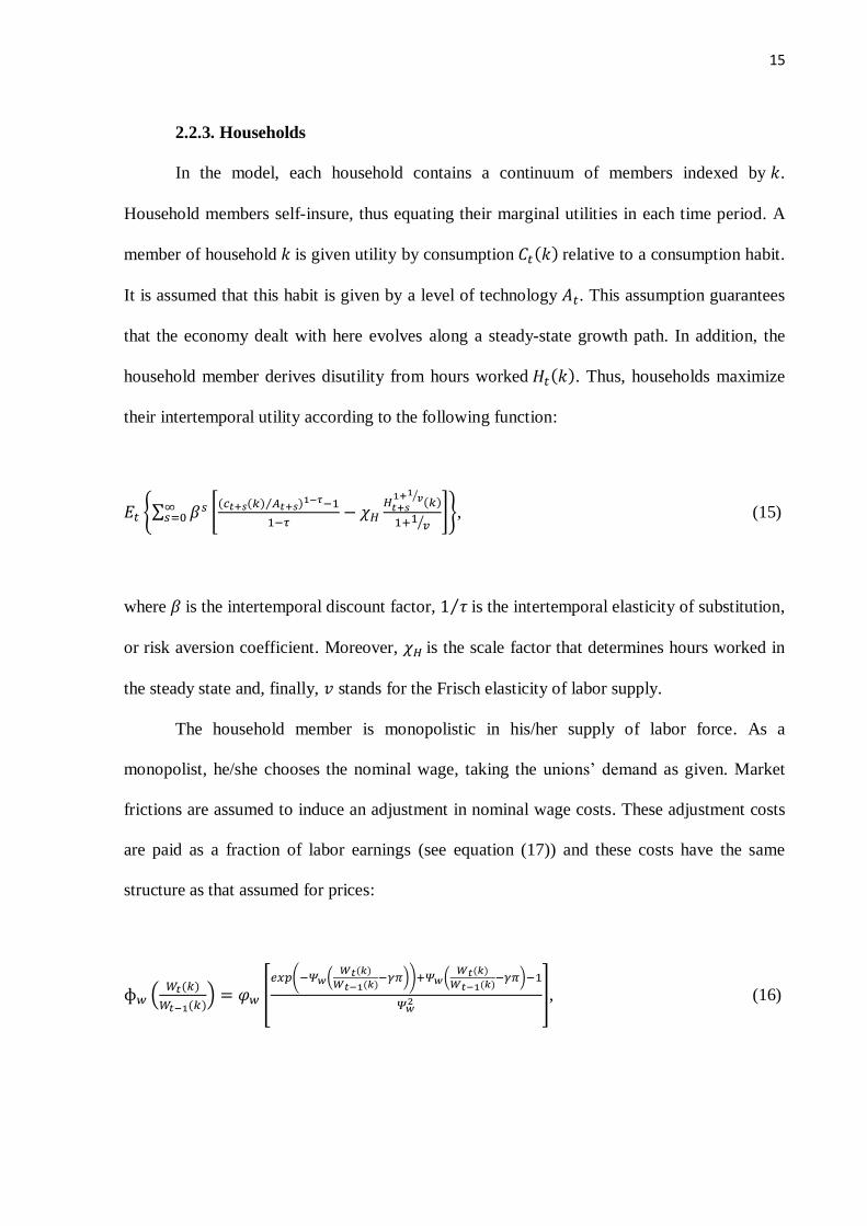
2.2.3. Households

In the model, each household contains a continuum of members indexed by 𝑘.

Household members self-insure, thus equating their marginal utilities in each time period. A

member of household 𝑘 is given utility by consumption 𝐶𝑡(𝑘) relative to a consumption habit.

It is assumed that this habit is given by a level of technology 𝐴𝑡. This assumption guarantees

that the economy dealt with here evolves along a steady-state growth path. In addition, the

household member derives disutility from hours worked 𝐻𝑡(𝑘). Thus, households maximize

their intertemporal utility according to the following function:

𝐸𝑡 {∑ 𝛽𝑠 [(𝑐𝑡+𝑠(𝑘) 𝐴𝑡+𝑠⁄ )1−𝜏−1

1−𝜏− 𝜒𝐻

𝐻𝑡+𝑠1+1

𝑣⁄(𝑘)

1+1𝑣⁄

]∞𝑠=0 }, (15)

where 𝛽 is the intertemporal discount factor, 1 𝜏⁄ is the intertemporal elasticity of substitution,

or risk aversion coefficient. Moreover, 𝜒𝐻 is the scale factor that determines hours worked in

the steady state and, finally, 𝑣 stands for the Frisch elasticity of labor supply.

The household member is monopolistic in his/her supply of labor force. As a

monopolist, he/she chooses the nominal wage, taking the unions’ demand as given. Market

frictions are assumed to induce an adjustment in nominal wage costs. These adjustment costs

are paid as a fraction of labor earnings (see equation (17)) and these costs have the same

structure as that assumed for prices:

ɸ𝑤 (𝑊𝑡(𝑘)

𝑊𝑡−1(𝑘)) = 𝜑𝑤 [

𝑒𝑥𝑝(−𝛹𝑤(𝑊𝑡(𝑘)

𝑊𝑡−1(𝑘)−𝛾𝜋))+𝛹𝑤(

𝑊𝑡(𝑘)

𝑊𝑡−1(𝑘)−𝛾𝜋)−1

𝛹𝑤2 ], (16)

16

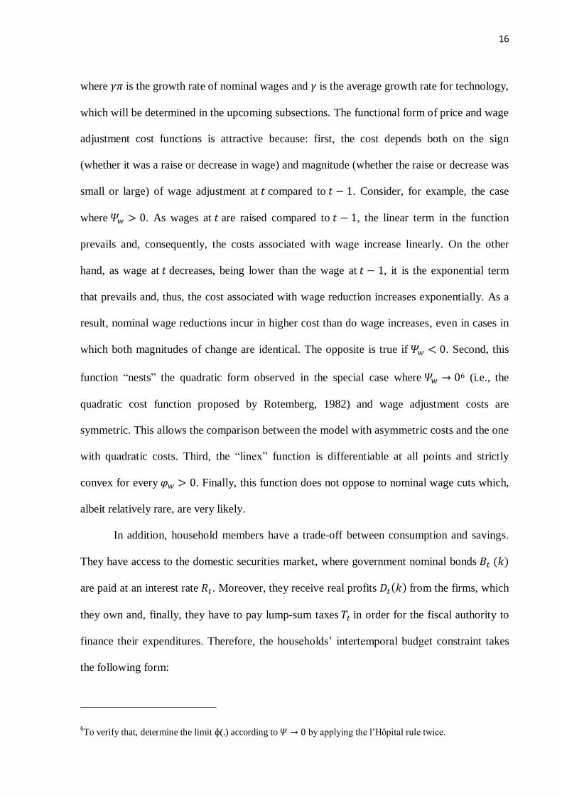
where 𝛾𝜋 is the growth rate of nominal wages and 𝛾 is the average growth rate for technology,

which will be determined in the upcoming subsections. The functional form of price and wage

adjustment cost functions is attractive because: first, the cost depends both on the sign

(whether it was a raise or decrease in wage) and magnitude (whether the raise or decrease was

small or large) of wage adjustment at 𝑡 compared to 𝑡 − 1. Consider, for example, the case

where 𝛹𝑤 > 0. As wages at 𝑡 are raised compared to 𝑡 − 1, the linear term in the function

prevails and, consequently, the costs associated with wage increase linearly. On the other

hand, as wage at 𝑡 decreases, being lower than the wage at 𝑡 − 1, it is the exponential term

that prevails and, thus, the cost associated with wage reduction increases exponentially. As a

result, nominal wage reductions incur in higher cost than do wage increases, even in cases in

which both magnitudes of change are identical. The opposite is true if 𝛹𝑤 < 0. Second, this

function “nests” the quadratic form observed in the special case where 𝛹𝑤 → 06 (i.e., the

quadratic cost function proposed by Rotemberg, 1982) and wage adjustment costs are

symmetric. This allows the comparison between the model with asymmetric costs and the one

with quadratic costs. Third, the “linex” function is differentiable at all points and strictly

convex for every 𝜑𝑤 > 0. Finally, this function does not oppose to nominal wage cuts which,

albeit relatively rare, are very likely.

In addition, household members have a trade-off between consumption and savings.

They have access to the domestic securities market, where government nominal bonds 𝐵𝑡 (𝑘)

are paid at an interest rate 𝑅𝑡. Moreover, they receive real profits 𝐷𝑡(𝑘) from the firms, which

they own and, finally, they have to pay lump-sum taxes 𝑇𝑡 in order for the fiscal authority to

finance their expenditures. Therefore, the households’ intertemporal budget constraint takes

the following form:

6To verify that, determine the limit ɸ(.) according to 𝛹 → 0 by applying the l’Hôpital rule twice.

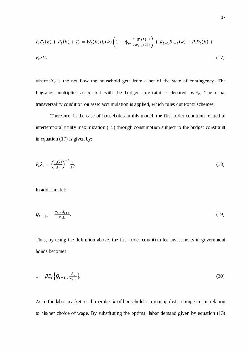
17

𝑃𝑡𝐶𝑡(𝑘) + 𝐵𝑡(𝑘) + 𝑇𝑡 = 𝑊𝑡(𝑘)𝐻𝑡(𝑘) (1 − ɸ𝑤 (𝑊𝑡(𝑘)

𝑊𝑡−1(𝑘))) + 𝑅𝑡−1𝐵𝑡−1(𝑘) + 𝑃𝑡𝐷𝑡(𝑘) +

𝑃𝑡𝑆𝐶𝑡, (17)

where 𝑆𝐶𝑡 is the net flow the household gets from a set of the state of contingency. The

Lagrange multiplier associated with the budget constraint is denoted by 𝜆𝑡. The usual

transversality condition on asset accumulation is applied, which rules out Ponzi schemes.

Therefore, in the case of households in this model, the first-order condition related to

intertemporal utility maximization (15) through consumption subject to the budget constraint

in equation (17) is given by:

𝑃𝑡𝜆𝑡 = (𝐶𝑡(𝑘)

𝐴𝑡)

−𝜏 1

𝐴𝑡. (18)

In addition, let:

𝑄𝑡+1|𝑡 =𝑃𝑡+1𝜆𝑡+1

𝑃𝑡𝜆𝑡. (19)

Thus, by using the definition above, the first-order condition for investments in government

bonds becomes:

1 = 𝛽𝐸𝑡 {𝑄𝑡+1|𝑡𝑅𝑡

𝜋𝑡+1}. (20)

As to the labor market, each member 𝑘 of household is a monopolistic competitor in relation

to his/her choice of wage. By substituting the optimal labor demand given by equation (13)

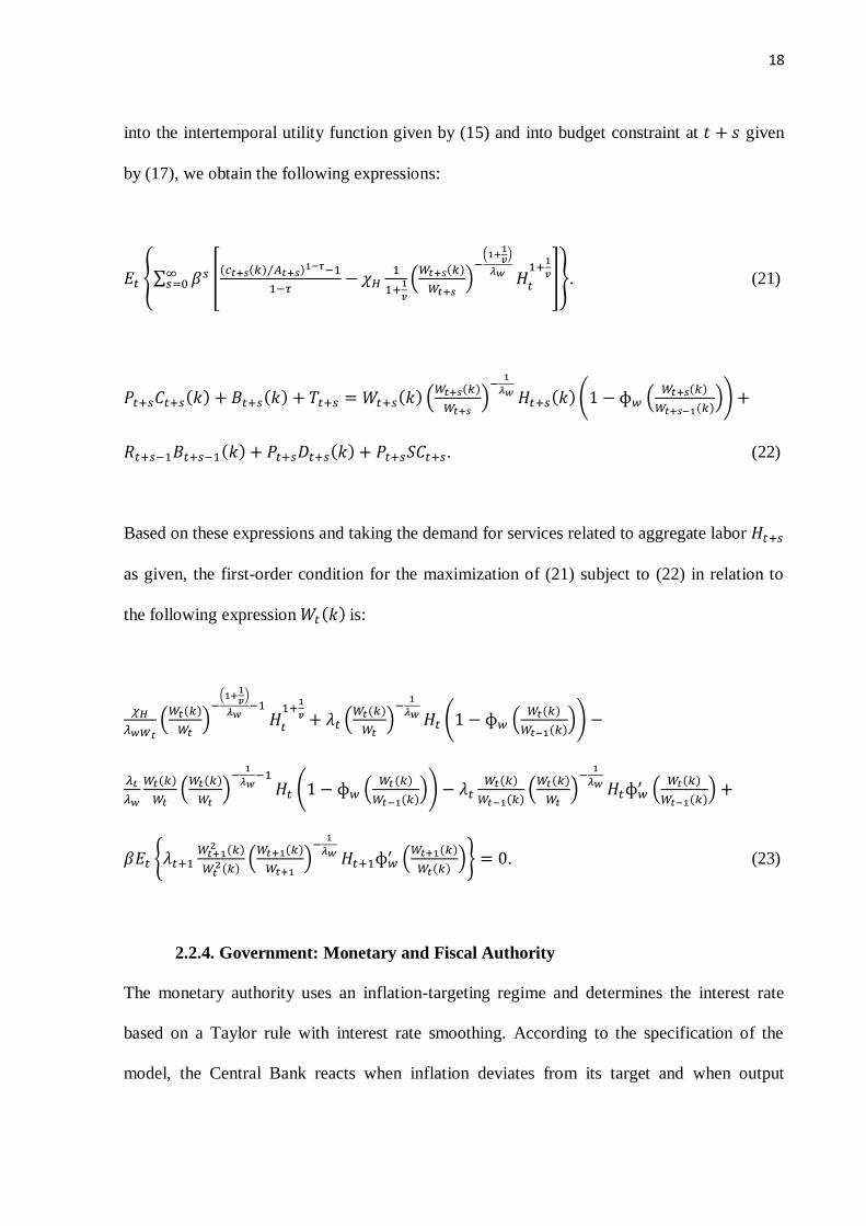
18

into the intertemporal utility function given by (15) and into budget constraint at 𝑡 + 𝑠 given

by (17), we obtain the following expressions:

𝐸𝑡 {∑ 𝛽𝑠 [(𝑐𝑡+𝑠(𝑘) 𝐴𝑡+𝑠⁄ )1−𝜏−1

1−𝜏− 𝜒𝐻

1

1+1

𝑣

(𝑊𝑡+𝑠(𝑘)

𝑊𝑡+𝑠)

−(1+

1𝑣

)

𝜆𝑤 𝐻𝑡

1+1

𝑣]∞𝑠=0 }. (21)

𝑃𝑡+𝑠𝐶𝑡+𝑠(𝑘) + 𝐵𝑡+𝑠(𝑘) + 𝑇𝑡+𝑠 = 𝑊𝑡+𝑠(𝑘) (𝑊𝑡+𝑠(𝑘)

𝑊𝑡+𝑠)

−1

𝜆𝑤 𝐻𝑡+𝑠(𝑘) (1 − ɸ𝑤 (𝑊𝑡+𝑠(𝑘)

𝑊𝑡+𝑠−1(𝑘))) +

𝑅𝑡+𝑠−1𝐵𝑡+𝑠−1(𝑘) + 𝑃𝑡+𝑠𝐷𝑡+𝑠(𝑘) + 𝑃𝑡+𝑠𝑆𝐶𝑡+𝑠. (22)

Based on these expressions and taking the demand for services related to aggregate labor 𝐻𝑡+𝑠

as given, the first-order condition for the maximization of (21) subject to (22) in relation to

the following expression 𝑊𝑡(𝑘) is:

𝜒𝐻

𝜆𝑤𝑊𝑡

(𝑊𝑡(𝑘)

𝑊𝑡)

−(1+

1𝑣

)

𝜆𝑤−1

𝐻𝑡

1+1

𝑣 + 𝜆𝑡 (𝑊𝑡(𝑘)

𝑊𝑡)

−1

𝜆𝑤 𝐻𝑡 (1 − ɸ𝑤 (𝑊𝑡(𝑘)

𝑊𝑡−1(𝑘))) −

𝜆𝑡

𝜆𝑤

𝑊𝑡(𝑘)

𝑊𝑡(

𝑊𝑡(𝑘)

𝑊𝑡)

−1

𝜆𝑤−1

𝐻𝑡 (1 − ɸ𝑤 (𝑊𝑡(𝑘)

𝑊𝑡−1(𝑘))) − 𝜆𝑡

𝑊𝑡(𝑘)

𝑊𝑡−1(𝑘)(

𝑊𝑡(𝑘)

𝑊𝑡)

−1

𝜆𝑤 𝐻𝑡ɸ𝑤′ (

𝑊𝑡(𝑘)

𝑊𝑡−1(𝑘)) +

𝛽𝐸𝑡 {𝜆𝑡+1𝑊𝑡+1

2 (𝑘)

𝑊𝑡2(𝑘)

(𝑊𝑡+1(𝑘)

𝑊𝑡+1)

−1

𝜆𝑤 𝐻𝑡+1ɸ𝑤′ (

𝑊𝑡+1(𝑘)

𝑊𝑡(𝑘))} = 0. (23)

2.2.4. Government: Monetary and Fiscal Authority

The monetary authority uses an inflation-targeting regime and determines the interest rate

based on a Taylor rule with interest rate smoothing. According to the specification of the

model, the Central Bank reacts when inflation deviates from its target and when output

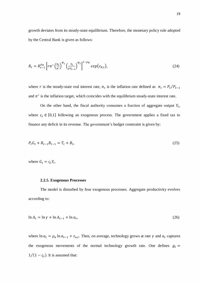
19

growth deviates from its steady-state equilibrium. Therefore, the monetary policy rule adopted

by the Central Bank is given as follows:

𝑅𝑡 = 𝑅𝑡−1𝜌𝑅 [𝑟𝜋∗ (

𝜋𝑡

𝜋∗)𝛹1

(𝑌𝑡

𝛾𝑌𝑡−1)

𝛹2

]1−𝜌𝑅

𝑒𝑥𝑝(휀𝑅,𝑡), (24)

where 𝑟 is the steady-state real interest rate, 𝜋𝑡 is the inflation rate defined as 𝜋𝑡 = 𝑃𝑡 𝑃𝑡−1⁄

and 𝜋∗ is the inflation target, which coincides with the equilibrium steady-state interest rate.

On the other hand, the fiscal authority consumes a fraction of aggregate output 𝑌𝑡,

where 𝜍𝑡 ∈ [0,1] following an exogenous process. The government applies a fixed tax to

finance any deficit in its revenue. The government’s budget constraint is given by:

𝑃𝑡𝐺𝑡 + 𝑅𝑡−1𝐵𝑡−1 = 𝑇𝑡 + 𝐵𝑡, (25)

where 𝐺𝑡 = 𝜍𝑡𝑌𝑡.

2.2.5. Exogenous Processes

The model is disturbed by four exogenous processes. Aggregate productivity evolves

according to:

ln 𝐴𝑡 = ln 𝛾 + ln 𝐴𝑡−1 + ln 𝑎𝑡, (26)

where ln 𝑎𝑡 = 𝜌𝑎 ln 𝑎𝑡−1 + 휀𝑎,𝑡. Then, on average, technology grows at rate 𝛾 and 𝑎𝑡 captures

the exogenous movements of the normal technology growth rate. One defines 𝑔𝑡 =

1 (1 − 𝜍𝑡)⁄ . It is assumed that:

20

ln 𝑔𝑡 = (1 − 𝜌𝑔) ln 𝑔 + 𝜌𝑔 ln 𝑔𝑡−1 + 휀𝑔,𝑡. (27)

The inverse elasticity of demand for intermediate goods evolves according to a logged

first-order autoregressive process:

ln 𝜆𝑝,𝑡 = (1 − 𝜌𝑝) ln 𝜆𝑝,𝑡−1 + 휀𝑝,𝑡. (28)

Finally, the monetary policy shock 휀𝑅,𝑡 is assumed to be serially uncorrelated. All

these four processes are independent and normally distributed with zero mean and standard

deviation 𝜎𝑧, 𝜎𝑔, 𝜎𝑝 and 𝜎𝑅.

2.3. Solution of the Model

The nonlinear nature often associated with DSGE models does not allow for their

closed analytical solution and, consequently, this nonlinearity implies a likelihood function7

that cannot be calculated analytically or numerically. To solve this problem, most of the

literature on dynamic economies has focused on approximate likelihood obtained from the

log-linearized version of the original model. When this approach is used, it is possible to use

the Kalman filter for constructing the likelihood function and its estimation. However,

linearization depends both on the accurate approximation of the model by a linear relationship

and on the assumption that economic shocks are normally distributed; but both hypotheses are

problematic. Firstly, the impact of linearization is stronger than it looks like. Fernández-

Villaverde, Rubio-Ramírez & Santos (2006) demonstrate that second-order errors in policy

7Recall that, as highlighted by An & Schorfheide (2007), likelihood-based inference is a useful tool that can take

dynamic steady-state models to real economic data.

21

functions may have first-order effects on the resulting likelihood function. Moreover, they

show that likelihood errors get worse as sample size increases; i.e., small errors in policy

functions accumulate at the same rate as sample size increases. Fernández-Villaverde &

Rubio-Ramírez (2005), Amisano & Tristani (2010), An & Schorfheide (2007), and Andreasen

(2011) use nonlinear approximations in their respective models and report that such

approximations provide a more appropriate fit of the data. Secondly, the hypothesis of normal

shocks hinders the investigation of models with time-varying volatility. Fernández-Villaverde

& Rubio-Ramírez (2007) use a model in which shocks are subject to stochastic volatility and

this induces both fundamental nonlinearities in the model and nonnormal distributions; in

addition, the authors argue that the use of a linear approximation method would eliminate the

effects of these shocks, not managing to explore this mechanism, requiring linear

approximation for the analysis of the model proposed by them. A similar case is observed in

the model proposed by Kim & Ruge-Murcia (2009) and extended by Aruoba, Bocola &

Shorfheide (2013), which was used in this paper. A linearized version of the model would

eliminate asymmetries in price and wage adjustment costs, which would not allow analyzing

the effects on the economy caused by the introduction of these rigidity mechanisms8.

Therefore, the use of a nonlinear approximation method to maintain the nonlinear structure of

the model is advisable.

So, before directing our attention to the estimation of the model, it is necessary to first

define the linear solution method to be used. As the solution method provides the policy

functions that will be used to calculate likelihood, which will strongly influence the

estimation, it is important to choose a method that is as accurate as possible. Nevertheless,

besides the fact that the method should be accurate, it is also important that it be quick, since

8 Aruoba, Bocola & Shorfheide (2013) demonstrated that the introduction of these asymmetries in price and

wage adjustment costs in the DSGE model explain very well the nonlinearities observed in prices and wages in the U.S. economy in the sample selected by them.

22

the likelihood function will be calculated several times for different sets of parameter values.

There is a wide range of methods for the linear approximation of a DSGE model, each of

them with advantages and disadvantages, as pointed out by Judd (1998). Additionally, the

nonlinear solution method can be based on local or global approximation. The perturbation

method is the one which is most widely used for the solution of dynamic models, which

builds a Taylor series expansion of the agents’ policy functions around the steady state and a

perturbation parameter. However, as argued by Aruoba, Fernández-Villaverde & Rubio-

Ramírez (2006), because it is a local approximation method, it is only satisfactory around the

steady state, i.e., this could be a problem in cases in which the economy is subject to large

shocks or is in crisis (e.g., the 1929 crisis or the 2008 financial crisis). On the other hand,

global methods are considered more robust, among which the most famous are the projection

methods, in which the policy functions corresponding to the model’s solution are represented

as a linear combination of previously known basis functions. As examples, we have the finite

element method, value function interaction, and spectral methods based on Chebyshev9

polynomials.

In brief, the nonlinear solution method chosen for the study is a second-order

perturbation method, accurate and quick, as reported by Aruoba, Fernández-Villaverde &

Rubio-Ramírez (2006). In addition, Moura (2010) tests several nonlinear approximation

methods using a simple real business cycle model and argues that global methods seem to be

the best approximation method, but the author warns that its implementation is way too

complicated and slower than perturbation methods. Hence, according to the author,

perturbation methods appear to yield a good trade-off between programming, computing time,

9Judd (1998), Miranda & Fackler (2002), DeJong & Dave (2007), and Aruoba, Fernández-Villaverde & Rubio-

Ramírez (2006) are good references on these methods. For further reading on perturbation methods, see Judd &

Guu (1997), Kim, Kim, Schumburg & Sims (2003), Schimitt-Grohé & Uribe (2004), and Gomme & Klein (2008).

23

and approximation accuracy. Therefore, although second-order perturbation methods do not

yield the best accuracy when the nonlinearity of the model is higher, this method is seemingly

the most attractive one, as it is the simplest and quickest to implement, which is important in

the case of DSGE models, in which for each set of parameter values, the model must be

solved as many times as necessary until it converts.

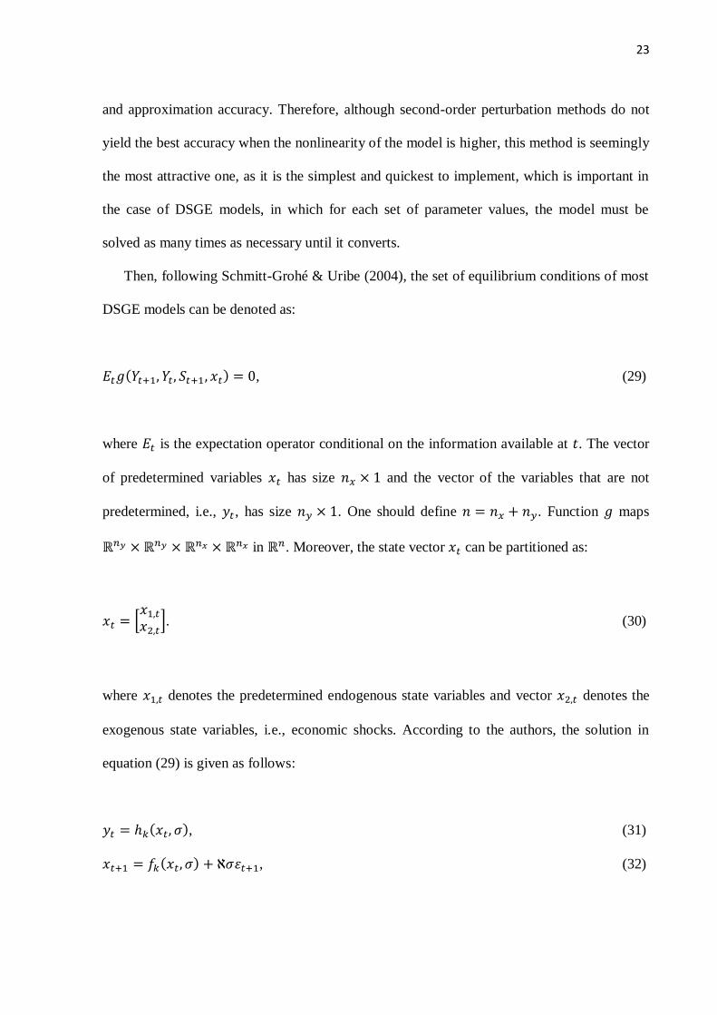
Then, following Schmitt-Grohé & Uribe (2004), the set of equilibrium conditions of most

DSGE models can be denoted as:

𝐸𝑡𝑔(𝑌𝑡+1, 𝑌𝑡, 𝑆𝑡+1, 𝑥𝑡) = 0, (29)

where 𝐸𝑡 is the expectation operator conditional on the information available at 𝑡. The vector

of predetermined variables 𝑥𝑡 has size 𝑛𝑥 × 1 and the vector of the variables that are not

predetermined, i.e., 𝑦𝑡, has size 𝑛𝑦 × 1. One should define 𝑛 = 𝑛𝑥 + 𝑛𝑦. Function 𝑔 maps

ℝ𝑛𝑦 × ℝ𝑛𝑦 × ℝ𝑛𝑥 × ℝ𝑛𝑥 in ℝ𝑛. Moreover, the state vector 𝑥𝑡 can be partitioned as:

𝑥𝑡 = [𝑥1,𝑡

𝑥2,𝑡]. (30)

where 𝑥1,𝑡 denotes the predetermined endogenous state variables and vector 𝑥2,𝑡 denotes the

exogenous state variables, i.e., economic shocks. According to the authors, the solution in

equation (29) is given as follows:

𝑦𝑡 = ℎ𝑘(𝑥𝑡, 𝜎), (31)

𝑥𝑡+1 = 𝑓𝑘(𝑥𝑡, 𝜎) + ℵ𝜎휀𝑡+1, (32)

24

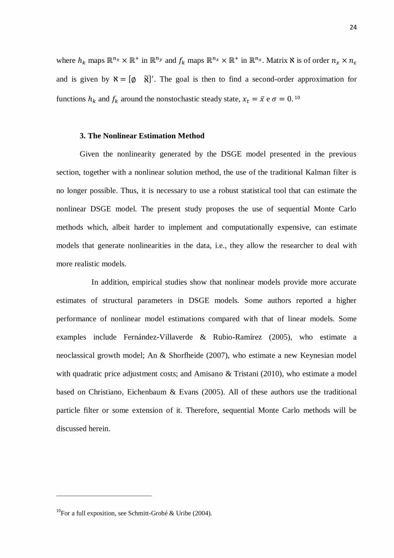
where ℎ𝑘 maps ℝ𝑛𝑥 × ℝ+ in ℝ𝑛𝑦 and 𝑓𝑘 maps ℝ𝑛𝑥 × ℝ+ in ℝ𝑛𝑥. Matrix ℵ is of order 𝑛𝑥 × 𝑛𝜀

and is given by ℵ = [∅ ℵ̃]′. The goal is then to find a second-order approximation for

functions ℎ𝑘 and 𝑓𝑘 around the nonstochastic steady state, 𝑥𝑡 = �̅� e 𝜎 = 0. 10

3. The Nonlinear Estimation Method

Given the nonlinearity generated by the DSGE model presented in the previous

section, together with a nonlinear solution method, the use of the traditional Kalman filter is

no longer possible. Thus, it is necessary to use a robust statistical tool that can estimate the

nonlinear DSGE model. The present study proposes the use of sequential Monte Carlo

methods which, albeit harder to implement and computationally expensive, can estimate

models that generate nonlinearities in the data, i.e., they allow the researcher to deal with

more realistic models.

In addition, empirical studies show that nonlinear models provide more accurate

estimates of structural parameters in DSGE models. Some authors reported a higher

performance of nonlinear model estimations compared with that of linear models. Some

examples include Fernández-Villaverde & Rubio-Ramírez (2005), who estimate a

neoclassical growth model; An & Shorfheide (2007), who estimate a new Keynesian model

with quadratic price adjustment costs; and Amisano & Tristani (2010), who estimate a model

based on Christiano, Eichenbaum & Evans (2005). All of these authors use the traditional

particle filter or some extension of it. Therefore, sequential Monte Carlo methods will be

discussed herein.

10For a full exposition, see Schmitt-Grohé & Uribe (2004).

25

3.1. Bayesian Estimation

Bayesian methods are good for estimating dynamic state problems. This approach

attempts to construct the state’s probability density function (pdf) by taking into consideration

all the information available up to the time of estimation. For a more specific problem, as is

the case of linear Gaussian estimation, the pdf remains Gaussian for each filter interaction,

and the Kalman filter reproduces and updates the mean and covariance of the distribution. On

the other hand, for nonlinear and/or non-Gaussian problems, there is no general analytical

expression (closed form) for the necessary pdf.

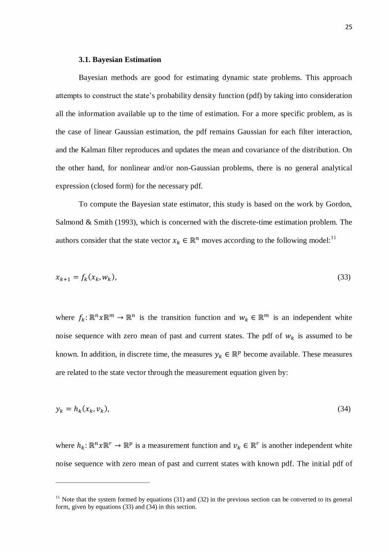
To compute the Bayesian state estimator, this study is based on the work by Gordon,

Salmond & Smith (1993), which is concerned with the discrete-time estimation problem. The

authors consider that the state vector 𝑥𝑘 ∈ ℝ𝑛 moves according to the following model:11

𝑥𝑘+1 = 𝑓𝑘(𝑥𝑘, 𝑤𝑘), (33)

where 𝑓𝑘: ℝ𝑛𝑥ℝ𝑚 → ℝ𝑛 is the transition function and 𝑤𝑘 ∈ ℝ𝑚 is an independent white

noise sequence with zero mean of past and current states. The pdf of 𝑤𝑘 is assumed to be

known. In addition, in discrete time, the measures 𝑦𝑘 ∈ ℝ𝑝 become available. These measures

are related to the state vector through the measurement equation given by:

𝑦𝑘 = ℎ𝑘(𝑥𝑘, 𝑣𝑘), (34)

where ℎ𝑘: ℝ𝑛𝑥ℝ𝑟 → ℝ𝑝 is a measurement function and 𝑣𝑘 ∈ ℝ𝑟 is another independent white

noise sequence with zero mean of past and current states with known pdf. The initial pdf of

11 Note that the system formed by equations (31) and (32) in the previous section can be converted to its general form, given by equations (33) and (34) in this section.

26

state vector 𝑝(𝑥1|𝐷0) ≡ 𝑝(𝑥1) is assumed to be available, as well as the functional forms 𝑓𝑖

and ℎ𝑖 for 𝑖 = 1, … , 𝑘. The information available up to period 𝑘 is the set of measures

𝐷𝑘 = {𝑦𝑖: 𝑖 = 1, … , 𝑘}.

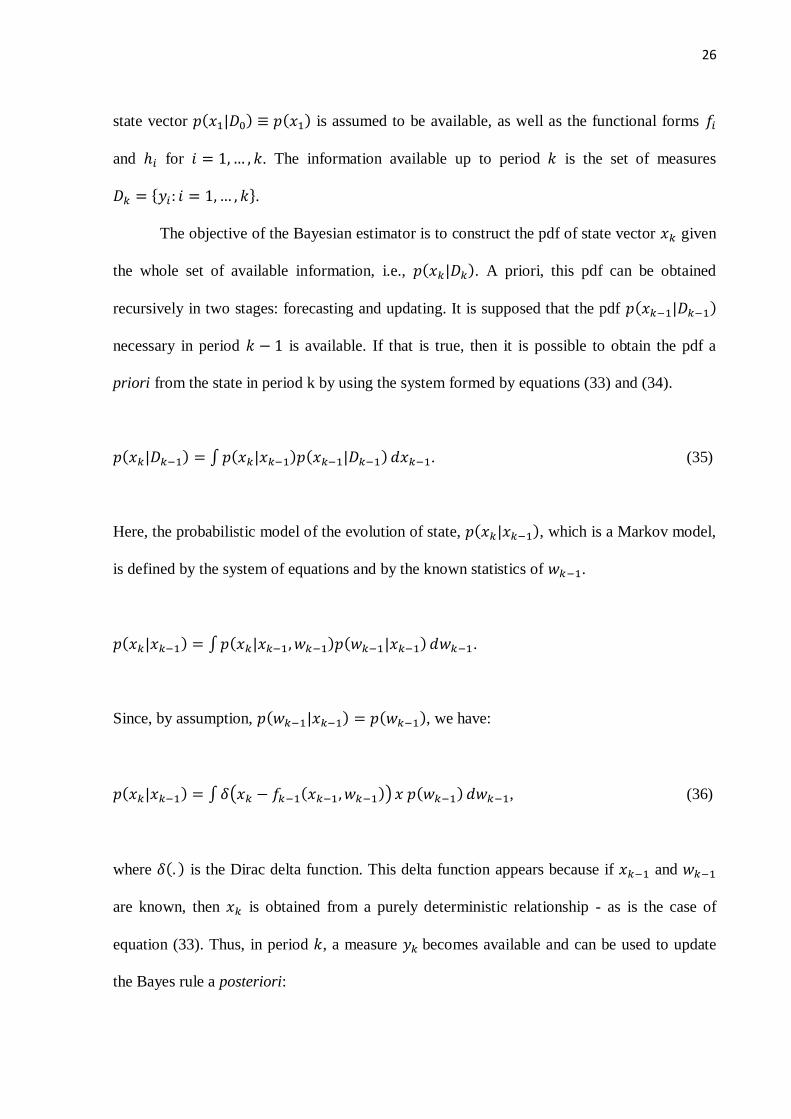
The objective of the Bayesian estimator is to construct the pdf of state vector 𝑥𝑘 given

the whole set of available information, i.e., 𝑝(𝑥𝑘|𝐷𝑘). A priori, this pdf can be obtained

recursively in two stages: forecasting and updating. It is supposed that the pdf 𝑝(𝑥𝑘−1|𝐷𝑘−1)

necessary in period 𝑘 − 1 is available. If that is true, then it is possible to obtain the pdf a

priori from the state in period k by using the system formed by equations (33) and (34).

𝑝(𝑥𝑘|𝐷𝑘−1) = ∫ 𝑝(𝑥𝑘|𝑥𝑘−1)𝑝(𝑥𝑘−1|𝐷𝑘−1) 𝑑𝑥𝑘−1. (35)

Here, the probabilistic model of the evolution of state, 𝑝(𝑥𝑘|𝑥𝑘−1), which is a Markov model,

is defined by the system of equations and by the known statistics of 𝑤𝑘−1.

𝑝(𝑥𝑘|𝑥𝑘−1) = ∫ 𝑝(𝑥𝑘|𝑥𝑘−1, 𝑤𝑘−1)𝑝(𝑤𝑘−1|𝑥𝑘−1) 𝑑𝑤𝑘−1.

Since, by assumption, 𝑝(𝑤𝑘−1|𝑥𝑘−1) = 𝑝(𝑤𝑘−1), we have:

𝑝(𝑥𝑘|𝑥𝑘−1) = ∫ 𝛿(𝑥𝑘 − 𝑓𝑘−1(𝑥𝑘−1, 𝑤𝑘−1)) 𝑥 𝑝(𝑤𝑘−1) 𝑑𝑤𝑘−1, (36)

where 𝛿(. ) is the Dirac delta function. This delta function appears because if 𝑥𝑘−1 and 𝑤𝑘−1

are known, then 𝑥𝑘 is obtained from a purely deterministic relationship - as is the case of

equation (33). Thus, in period 𝑘, a measure 𝑦𝑘 becomes available and can be used to update

the Bayes rule a posteriori:

27

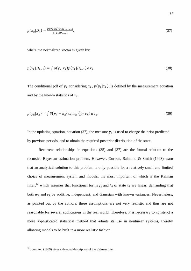
𝑝(𝑥𝑘|𝐷𝑘) =𝑝(𝑦𝑘|𝑥𝑘)𝑝(𝑥𝑘|𝐷𝑘−1)

𝑝(𝑦𝑘|𝐷𝑘−1), (37)

where the normalized vector is given by:

𝑝(𝑦𝑘|𝐷𝑘−1) = ∫ 𝑝(𝑦𝑘|𝑥𝑘)𝑝(𝑥𝑘|𝐷𝑘−1) 𝑑𝑥𝑘. (38)

The conditional pdf of 𝑦𝑘 considering 𝑥𝑘, 𝑝(𝑦𝑘|𝑥𝑘), is defined by the measurement equation

and by the known statistics of 𝑣𝑘

𝑝(𝑦𝑘|𝑥𝑘) = ∫ 𝛿(𝑦𝑘 − ℎ𝑘(𝑥𝑘, 𝑣𝑘))𝑝 (𝑣𝑘) 𝑑𝑣𝑘 . (39)

In the updating equation, equation (37), the measure 𝑦𝑘 is used to change the prior predicted

by previous periods, and to obtain the required posterior distribution of the state.

Recurrent relationships in equations (35) and (37) are the formal solution to the

recursive Bayesian estimation problem. However, Gordon, Salmond & Smith (1993) warn

that an analytical solution to this problem is only possible for a relatively small and limited

choice of measurement system and models, the most important of which is the Kalman

filter,12

which assumes that functional forms 𝑓𝑘 and ℎ𝑘 of state 𝑥𝑘 are linear, demanding that

both 𝑤𝑘 and 𝑣𝑘 be additive, independent, and Gaussian with known variances. Nevertheless,

as pointed out by the authors, these assumptions are not very realistic and thus are not

reasonable for several applications in the real world. Therefore, it is necessary to construct a

more sophisticated statistical method that admits its use in nonlinear systems, thereby

allowing models to be built in a more realistic fashion.

12 Hamilton (1989) gives a detailed description of the Kalman filter.

28

There exist a few alternatives to deal with this problem, including two improvements

of the traditional Kalman filter, in an attempt to make the estimation of nonlinear systems

better, namely the Extended Kalman Filter (EKF) and the Unscented Kalman Filter (UKF).

According to Simon (2006), the EKF is the state estimation algorithm most widely used in

nonlinear systems. Anyway, the author warns that this filter may be hard to adjust and, more

often than not, yields unreliable estimates in cases of severe nonlinearity. That occurs because

the filter relies on linearization to propagate state means and covariance. On the other hand,

the UKF provides remarkable improvements in the accuracy of estimates when compared

with the EKF; but the UKF is only an approximate nonlinear estimator. In other words, the

EKF calculates the mean of a nonlinear system with first-order accuracy, whereas the UKF

improves that by yielding an estimate with higher-order accuracy. Notwithstanding, Simon

(2006) comments that the use of these filters simply delays the inevitable disparity that is

observed when the nonlinear measurement system is too severe.

Hence, the method used herein, i.e., the particle filter (fully nonlinear state estimator),

introduced in what follows, is proposed with the aim of improving the estimation of DSGE

models, thus bringing these theoretical models closer to the reality of economic data.

3.2. Particle filter

The particle filter – also known as sequential importance sampling method or simply

as sequential Monte Carlo method, is introduced here. It is a fully nonlinear numerical state

estimator that may be used to estimate any model in state-space form. According to Simon

(2006), the particle filter, or Monte Carlo filter, is a “brute force” statistical estimation method

that often works well with problems that are not easily dealt with by the conventional Kalman

filter, that is, highly nonlinear systems.

29

The particle filter was originally introduced by Metropolis & Ulam (1949), who

described the mathematical treatment of physical phenomena. According to those authors,

problems involving just some particles, through the analysis of ordinary differential equation

systems, were investigated in classic mechanics. However, as argued by the authors, a totally

different technique is necessary for the description of systems with a large number of

particles, the so-called method of statistical mechanics, which focuses on the analysis of the

properties of a set of particles rather than on the observation of individual particles. Note that

the particle filter is an improvement of the SIS (sequential importance sampling) algorithm. It

is the foundation on which the literature on the subsequent sequential Monte Carlo methods

rests. According to Arulampalam et al. (2002), the SIS algorithm suffers from a degeneracy

problem, in which, after some interactions, only one of all initial particles has a non-negligible

weight and therefore all Monte Carlo estimations of the integrals are made using a sample of

size 1. Conversely, the particle filter proposed by Gordon, Salmond & Smith (1993) and

Kitagawa (1996) is considered to be the standard Monte Carlo method. This filter, which

Arulampalam et al. (2002) later called generic particle filter, adds a resampling step to the

algorithm, which helps reduce the degeneracy observed in the SIS algorithm. Despite its

broad use in several other areas of research,13

just recently has the particle filter begun to be

used as a statistical tool to calculate likelihood in nonlinear models in economics. For

instance, Kim, Shephard & Chib (1998) and Pit & Shepard (1999) applied this method to

stochastic volatility models. However, pioneering research into the use of particle filters in

DSGE models was conducted by Fernández-Villaverde & Rubio-Ramírez (2005). By blazing

the trail for the use of particle filter to estimate macroeconomic models, other similar works

were introduced into the literature on DSGE models involving sequential Monte Carlo

methods: An (2007), An & Schorfheide (2007), Fernández-Villaverde & Rubio-Ramírez

13See Cox (1996) for an application of the particle filter to mobile robot localization.

30

(2007), Flury & Shephard (2011), Amisano & Tristani (2010), DeJong et al. (2009), Strid

(2006), Andreasen (2011), Fasolo (2012), and Aruoba, Bocola & Shorfheide (2013).

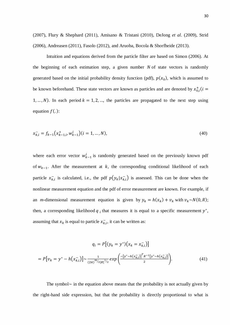
Intuition and equations derived from the particle filter are based on Simon (2006). At

the beginning of each estimation step, a given number 𝑁 of state vectors is randomly

generated based on the initial probability density function (pdf), 𝑝(𝑥0), which is assumed to

be known beforehand. These state vectors are known as particles and are denoted by 𝑥0,𝑖+ (𝑖 =

1, … , 𝑁). In each period 𝑘 = 1, 2, …, the particles are propagated to the next step using

equation 𝑓(. ):

𝑥𝑘,𝑖− = 𝑓𝑘−1(𝑥𝑘−1,𝑖

+ , 𝑤𝑘−1𝑖 )(𝑖 = 1, … , 𝑁), (40)

where each error vector 𝑤𝑘−1𝑖 is randomly generated based on the previously known pdf

of 𝑤𝑘−1. After the measurement at 𝑘, the corresponding conditional likelihood of each

particle 𝑥𝑘,𝑖− is calculated, i.e., the pdf 𝑝(𝑦𝑘|𝑥𝑘,𝑖

− ) is assessed. This can be done when the

nonlinear measurement equation and the pdf of error measurement are known. For example, if

an m-dimensional measurement equation is given by 𝑦𝑘 = ℎ(𝑥𝑘) + 𝑣𝑘 with 𝑣𝑘~𝑁(0, 𝑅);

then, a corresponding likelihood 𝑞 𝑖 that measures it is equal to a specific measurement 𝑦∗,

assuming that 𝑥𝑘 is equal to particle 𝑥𝑘,𝑖− , it can be written as:

𝑞𝑖 = 𝑃[(𝑦𝑘 = 𝑦∗)(𝑥𝑘 = 𝑥𝑘,𝑖− )]

= 𝑃[𝑣𝑘 = 𝑦∗ − ℎ(𝑥𝑘,𝑖− )]~

1

(2𝜋)𝑚

2⁄ |𝑅|1

2⁄𝑒𝑥𝑝 (

−[𝑦∗−ℎ(𝑥𝑘,𝑖− )]

𝑇𝑅−1[𝑦∗−ℎ(𝑥𝑘,𝑖

− )]

2). (41)

The symbol~ in the equation above means that the probability is not actually given by

the right-hand side expression, but that the probability is directly proportional to what is

31

found on the right hand side of the equation. Thus, if this equation is used for all

particles 𝑥𝑘,𝑖− (𝑖 = 1, … , 𝑁), the corresponding likelihoods that the state is equal in each

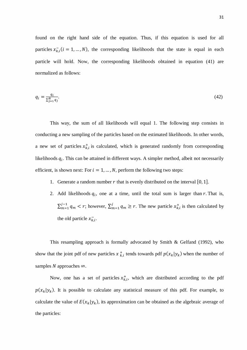
particle will hold. Now, the corresponding likelihoods obtained in equation (41) are

normalized as follows:

𝑞𝑖 =𝑞𝑖

∑ 𝑞𝑗𝑁𝑗=1

. (42)

This way, the sum of all likelihoods will equal 1. The following step consists in

conducting a new sampling of the particles based on the estimated likelihoods. In other words,

a new set of particles 𝑥𝑘,𝑖+ is calculated, which is generated randomly from corresponding

likelihoods 𝑞𝑖 . This can be attained in different ways. A simpler method, albeit not necessarily

efficient, is shown next: For 𝑖 = 1, … , 𝑁, perform the following two steps:

1. Generate a random number 𝑟 that is evenly distributed on the interval [0, 1].

2. Add likelihoods 𝑞𝑖, one at a time, until the total sum is larger than 𝑟. That is,

∑ 𝑞𝑚 < 𝑟𝑗−1𝑚=1 ; however, ∑ 𝑞𝑚 ≥ 𝑟

𝑗𝑚=1 . The new particle 𝑥𝑘,𝑖

+ is then calculated by

the old particle 𝑥𝑘,𝑖− .

This resampling approach is formally advocated by Smith & Gelfand (1992), who

show that the joint pdf of new particles 𝑥 𝑘,𝑖+ tends towards pdf 𝑝(𝑥𝑘|𝑦𝑘) when the number of

samples 𝑁 approaches ∞.

Now, one has a set of particles 𝑥𝑘,𝑖+ , which are distributed according to the pdf

𝑝(𝑥𝑘|𝑦𝑘). It is possible to calculate any statistical measure of this pdf. For example, to

calculate the value of 𝐸(𝑥𝑘|𝑦𝑘), its approximation can be obtained as the algebraic average of

the particles:

32

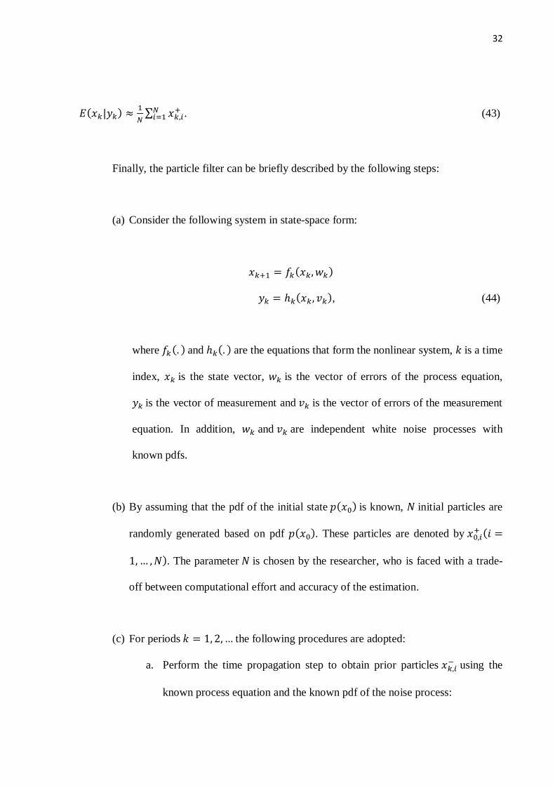
𝐸(𝑥𝑘|𝑦𝑘) ≈1

𝑁∑ 𝑥𝑘,𝑖

+𝑁𝑖=1 . (43)

Finally, the particle filter can be briefly described by the following steps:

(a) Consider the following system in state-space form:

𝑥𝑘+1 = 𝑓𝑘(𝑥𝑘, 𝑤𝑘)

𝑦𝑘 = ℎ𝑘(𝑥𝑘, 𝑣𝑘), (44)

where 𝑓𝑘 (. ) and ℎ𝑘(. ) are the equations that form the nonlinear system, 𝑘 is a time

index, 𝑥𝑘 is the state vector, 𝑤𝑘 is the vector of errors of the process equation,

𝑦𝑘 is the vector of measurement and 𝑣𝑘 is the vector of errors of the measurement

equation. In addition, 𝑤𝑘 and 𝑣𝑘 are independent white noise processes with

known pdfs.

(b) By assuming that the pdf of the initial state 𝑝(𝑥0) is known, 𝑁 initial particles are

randomly generated based on pdf 𝑝(𝑥0). These particles are denoted by 𝑥0,𝑖+ (𝑖 =

1, … , 𝑁). The parameter 𝑁 is chosen by the researcher, who is faced with a trade-

off between computational effort and accuracy of the estimation.

(c) For periods 𝑘 = 1, 2, … the following procedures are adopted:

a. Perform the time propagation step to obtain prior particles 𝑥𝑘,𝑖− using the

known process equation and the known pdf of the noise process:

33

𝑥𝑘,𝑖− = 𝑓𝑘−1(𝑥𝑘−1,𝑖

+ , 𝑤𝑘−1𝑖 )(𝑖 = 1, … , 𝑁), (45)

where each vector of errors 𝑤𝑘−1 𝑖 is generated randomly based on the

known pdf of 𝑤𝑘−1.

b. Calculate likelihood 𝑞𝑖 of each particle 𝑥𝑘,𝑖− conditioned on the vector of

measurement 𝑦𝑘 . That is done by assessing the pdf 𝑝(𝑦𝑘|𝑥𝑘,𝑖− ) based on the

nonlinear measurement equation and on the pdf of the measurement

equation errors.

c. Normalize the corresponding likelihoods obtained in the previous steps as

follows:

𝑞𝑖 =𝑞𝑖

∑ 𝑞𝑗𝑁𝑗=1

. (46)

Now the sum of all likelihoods equals 1.

d. A set of posterior particles 𝑥𝑘,𝑖+ is generated based on corresponding

likelihoods 𝑞𝑖. This is the resampling step.

Now that a set of particles 𝑥𝑘,𝑖 + was obtained, distributed according to pdf 𝑝(𝑥𝑘|𝑦𝑘), the

researcher can calculate the statistical measures (often mean and covariance) of this pdf.

Finally, the rationale behind the particle filter is that the particles generated from

distribution 𝑝(𝑥0) which do not contribute to characterizing the state vector in each time

34

period should be eliminated, leaving only those particles that have a larger weight on the

distribution. Therefore, the filter includes only the particles around the relevant regions of the

state space. Hence, the sampling step is the key element of the particle filter, based on a slight

modification in the standard of the SIS method. In the case of the standard importance

sampling method, each particle generated in the projection step would be sampled with the

same probability. However, it is known from the literature on the sequential Monte Carlo

method that when 𝑡 → ∞, there is a degeneracy problem, in which, except for a single specific

particle, all the other weights converge to zero. Moreover, even the single particle with weight

equal to 1 does not necessarily provide the best description of the state vector. Accordingly,

the modification proposed and later used by Fernández-Villaverde & Rubio-Ramírez (2005) is

of great importance to the proper operation of the particle filter.

3.3. Problems involving the particle filter and its alternatives

The literature on the sequential Monte Carlo methods underscores that the standard

particle filter suffers from the so-called “sample impoverishment,”14

which may be regarded

as a milder degeneracy problem, i.e., less harmful to the method. Note that the sample of a

very large number of particles will not degenerate as occurs with the SIS algorithm; however,

this number will decrease for only some distinct particle values. Sample impoverishment

occurs mainly when there are outliers in the data or in situations in which the measurement

equation gives a lot of information about the states. Pitt & Shephard (1999) comment that the

presence of outliers in the data often requires higher values for the number of particles in

14To calculate the inefficiency of the particle filter (how severe sample impoverishment is) and to calculate the

quality of the approximation to the state density with the particle filter, Arulampalam et al. (2002) suggest

estimating the so-called effective sample size. The idea is to use the variance of importance weights as a tool to

assess the quality of the distribution. This statistic is given by:

𝑁𝑒𝑓𝑓 =1

∑ (𝑞𝑡𝑖)

2𝑁𝑖=1

.

35

order to generate a good approximation to the density. Moreover, as commented by Moura

(2010), the importance sampler used to approximate the integrals in the filtering process only

includes the information available in the observed variables at 𝑡 − 1, not using the

information at 𝑡. Accordingly, some extensions to the standard particle filter were proposed in

order to include information available at 𝑡, making it more efficient, for instance, the auxiliary

particle filter proposed by Pitt & Shephard (1999) and the conditional particle filter

introduced by Amisano & Tristani (2010). However, it should be highlighted that the

consistency of the particle filter is based mainly on the number of particles used to

approximate the probability density function to the state variables in each time period.

Nevertheless, there is a trade-off between the accuracy of the filter and the time necessary to

perform the procedure. Fasolo (2012) shows that the log likelihood values become more

accurate as the number of particles increases. Additionally, the author compares the

performance of the standard particle filter and of the auxiliary one and concludes that, in spite

of the latter having a good performance when the number of observations is large and the

number of particles is relatively small, the standard particle filter is significantly less

computationally demanding and, therefore, this filter tends to have a better performance with

a large number of particles in comparison with the auxiliary filter.

Therefore, there are some extensions to the standard particle filter aimed at improving

its performance. Nonetheless, the particle filter proposed by Fernández-Villaverde & Rubio-

Ramírez (2005 and 2007) is still a robust statistical tool with better results than the traditional

Kalman filter, as demonstrated by Fernández-Villaverde & Rubio-Ramírez (2005), An &

Schorfheide (2007), and Amisano & Tristani (2010).

36

3.4. Posterior distribution simulations

After obtaining the likelihood, it may be used in a Bayesian algorithm that simulates

the posteriors of the parameters. In the present paper, the algorithm known as Random-Walk

Metropolis (RWM) introduced in Chib (2001) and in An & Schorfheide (2007) is used.

Briefly put, sequential Monte Carlo methods are used to calculate the likelihood of the DSGE

model, and then this likelihood is plugged into a Monte Carlo Markov Chain (MCMC)

process.

So as to carry out this process successfully, first one estimates the linearized version of

the DSGE model introduced in Section 2 using the RWM algorithm. By using the same

covariance matrix for the distribution proposed to generate the particles, as in the case of the

linearized DSGE model, we then run the RWM algorithm based on the likelihood function

associated with the second-order approximation of the DSGE model. Note that the covariance

matrix of the proposed distribution is defined such that the RWM algorithm will have an

acceptance rate around 50%. A total of 100,000 particles are used to approximate the

likelihood function of the nonlinear DSGE model, whereas the variance of measurement

errors is defined as 10% of the variance of the observation sample. Finally, 275,000

simulations of the posterior distribution of the nonlinear DSGE model are obtained. It should

be underscored that the first 75,000 simulations are eliminated and that only the statistical

results obtained from the remaining simulations are reported.

Also, the number of particles chosen in the present paper is much larger than that

observed in previous studies. For example, Fernández-Villaverde & Rubio-Ramírez (2005)

use 60,000 particles in the neoclassical growth model. Afterwards, the same authors use an

extended version of this model with 80,000 particles. On the other hand, An & Schorfheide

(2007) estimate a new Keynesian model with 40,000 particles. Finally, Aruoba, Bocola &

Shorfheide (2013) use 80,000 particles to calculate the likelihood function of a DSGE model

37

with asymmetric adjustment costs for both prices and wages. Therefore, in this paper, we used

the “brute force” approach to tackle the afore-mentioned impoverishment problem. Despite

the higher computational costs, the increase in the number of particles helps minimize the

impoverishment problem.

4. Estimation and Results

After the discussion on the methods for solution of the DSGE model and also on the

estimation methods, the present section deals with the empirical results of the proposed

model. The model shown in Section 2 is solved using a nonlinear method and its structural

parameters are estimated by the particle filter. The estimation results obtained through the

Kalman filter for the linearized version of the model are briefly described. However, no

comparison is made between the performance of the two filters, as in other studies such as An

& Schorfheide (2007) and Amisano & Tristani (2010). Therefore, the first part of this section

shows the data and prior distributions. The second part is concerned with posterior

distributions, comments on the results, and compares the parameters with other literature data.

Finally, the section concludes by analyzing the impulse response functions aiming to assess

the dynamics of the economy in its linear version (symmetric rigidity) and in its linear version

(asymmetric rigidity) in the presence of a transient shock to the monetary and fiscal policies.

4.1. Data and prior distributions

This paper uses quarterly data from 2000:1 to 2014:4, totaling 60 observations. Note

that the selection of this period is due to a regime shift, with the introduction of the inflation-

targeting regime in 1999. Four observable macroeconomic variables were utilized: output,

inflation, interest rate, and wages. The GDP, IPCA (broad consumer price index) and the

Selic interest rate data published by the Brazilian Institute of Geography and Statistics (IBGE)

38

were used. Average earnings, a labor market variable disclosed by DIEESE, were used. This

indicator uses the behavior of the metropolitan area of São Paulo as proxy for the national

dynamics. The decision to adopt this series rather than that published by the IBGE was based

on the structural break in this series in 2002 caused by a methodological change.

The priors were estimated following economic studies conducted in Brazil, and in the

case of parameters that had not been calculated for the Brazilian economy, the same prior of

the original model was used. The estimation of parameter β was based on Shorfheide (2000).

The mean value for parameter 𝑣 was set as 2. We chose the value 1.30 for τ, which is

employed in the SAMBA model by Castro et al. (2011). The values of monetary authority

parameters (𝜌𝑟, 𝛹2 and 𝛹2) were the same as those of the SAMBA model. As to shock

persistence parameters (𝜌𝑎, 𝜌𝑔 and 𝜌𝑝), the prior was equal to 0.85. The values of rigidity

parameters are the same described in Aruoba, Bocola & Shorfheide (2013), since there is no

empirical evidence regarding these parameters in the Brazilian economy. Finally, the inverse

gamma distribution was chosen for all standard deviations. Tables 4.1 and 4.2 summarize the

priors used for the parameters.

4.2. Estimation results: linear and nonlinear models

First of all, this subsection briefly presents the results for the estimation made using

the Kalman filter. The first step consisted in finding the solution to the model shown in

Section 2 by a linear approximation via Taylor expansions or logarithmic approximations.

After linearization, the solution to the model is written as deviation of the values from the

steady state and the model is given in difference equation form with rational expectations. The

next step consisted in writing the solution in state-space form, assessing the likelihood

function via the Kalman filter. The parameters estimated by this method will not be analyzed

thoroughly as the focus is on the result of the nonlinear model. Nevertheless, as demonstrated

39

in Table 4.1, the estimated parameters appear to be in line with the results obtained for the

Brazilian economy, except for the interest rate smoothing parameter, whose value was

apparently way below that observed by Castro et al. (2011) and Sin & Gaglianone (2006). On

the other hand, the value obtained for 𝛽 was smaller than the usual one often calculated for

Brazil (around 0.989).

However, the most important task to be accomplished in this section concerns the

analysis of the results obtained for the estimation made using the particle filter. Unlike

previous findings, the DSGE model is solved by using a second-order perturbation method,

which results in a nonlinear representation in state-space form. In this case, it is no longer

possible to use the Kalman filter to assess the likelihood function. Table 4.2 shows the results

for the estimation made using the particle filter.

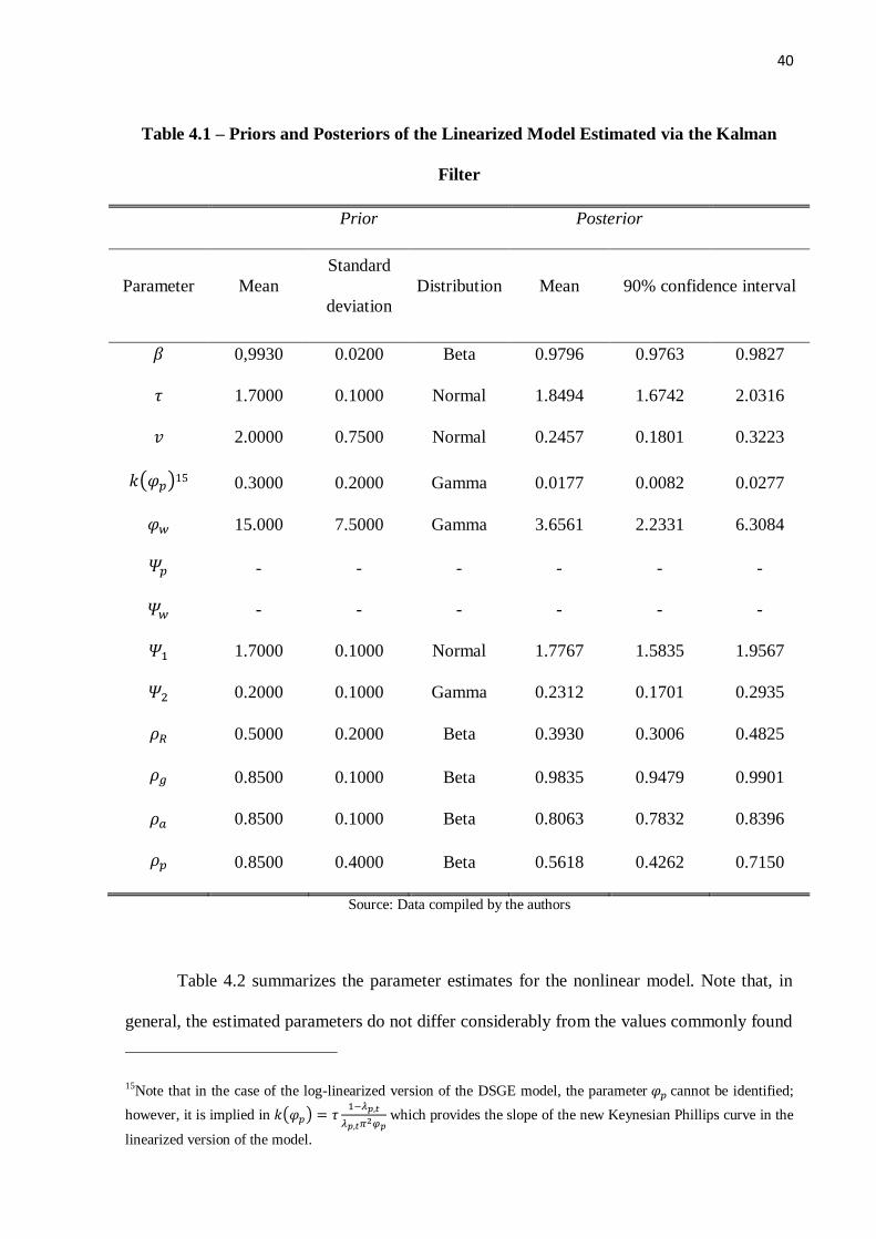
40

Table 4.1 – Priors and Posteriors of the Linearized Model Estimated via the Kalman

Filter

Prior Posterior

Parameter Mean

Standard

deviation

Distribution Mean 90% confidence interval

𝛽 0,9930 0.0200 Beta 0.9796 0.9763 0.9827

𝜏 1.7000 0.1000 Normal 1.8494 1.6742 2.0316

𝑣 2.0000 0.7500 Normal 0.2457 0.1801 0.3223

𝑘(𝜑𝑝)15 0.3000 0.2000 Gamma 0.0177 0.0082 0.0277

𝜑𝑤 15.000 7.5000 Gamma 3.6561 2.2331 6.3084

𝛹𝑝 - - - - - -

𝛹𝑤 - - - - - -

𝛹1 1.7000 0.1000 Normal 1.7767 1.5835 1.9567

𝛹2 0.2000 0.1000 Gamma 0.2312 0.1701 0.2935

𝜌𝑅 0.5000 0.2000 Beta 0.3930 0.3006 0.4825

𝜌𝑔 0.8500 0.1000 Beta 0.9835 0.9479 0.9901

𝜌𝑎 0.8500 0.1000 Beta 0.8063 0.7832 0.8396

𝜌𝑝 0.8500 0.4000 Beta 0.5618 0.4262 0.7150

Source: Data compiled by the authors

Table 4.2 summarizes the parameter estimates for the nonlinear model. Note that, in

general, the estimated parameters do not differ considerably from the values commonly found

15Note that in the case of the log-linearized version of the DSGE model, the parameter 𝜑𝑝 cannot be identified;

however, it is implied in 𝑘(𝜑𝑝) = 𝜏1−𝜆𝑝,𝑡

𝜆𝑝,𝑡𝜋2𝜑𝑝 which provides the slope of the new Keynesian Phillips curve in the

linearized version of the model.

41

in the empirical literature with Brazilian data. The first part of Table 4.2 shows the statistics

for household preferences. The intertemporal discount factor, 𝛽, was equal to 0.9951, smaller

than the values commonly calibrated (0.989) for the Brazilian economy described by Castro et

al. (2011) and Vasconcelos & Divino (2012). Conversely, parameter 𝜏 – which measures the

inverse intertemporal elasticity of substitution and is also known as risk aversion coefficient –

yielded an estimate of 1.8480, higher than that obtained by Portugal & Silva (2011) and

Castro et al. (2011). Interestingly, empirical models, such as those published by the Central

Bank of Brazil in its quarterly inflation reports, show that the interest rate eventually produces

a small effect on inflation compared with the effects observed in DSGE models seen in

impulse response functions. Finally, the elasticity of labor supply, 𝑣, yielded a value of

0.1692, indicating wage rigidity in the specification of the model after the introduction of

asymmetric wage adjustment costs.

As to the monetary policy coefficients, the Central Bank of Brazil seemingly attaches

more weight to the deviations in inflation than in output. The estimated parameter that

responds to inflation, 𝛹1, yielded 1.6220. This value was smaller than that observed by Casto

et al. (2011), i.e., 2.43. However, it was higher than that obtained by Sin & Gaglianone

(2006), 1.33, and Santos & Kanczuk (2011), 1.50. The value of parameter 𝛹2, which indicates

the importance given by the Central Bank to the deviation from output, was 0.3905, much

higher than that observed by the afore-mentioned authors – 0.16, 0.13, and 0.16, respectively.

The estimated parameters demonstrate that, although the Central Bank attaches more weight

to inflation than to output, in the case of the model used here, the monetary authority gives

considerable attention to deviations from output, which occurs in a lesser degree in most

empirical studies on Brazil. Nonetheless, according to this finding, the monetary authority

reacts to output when it is above its potential so as to prevent higher inflation rates caused by

excess demand. Finally, the interest rate smoothing coefficient, 𝜌𝑟, corresponded to 0.7419,

42

which is lower than that reported by Castro et al. (2011) and by Sin & Gaglione (2006), who

obtained 0.79 and 0.8402, respectively. This indicates that the monetary authority takes into

account the previous interest rate level in order to make decisions about its increase. In other

words, the Central Bank usually keeps the interest rate stable over time instead of changing it

abruptly. In sum, the results found here indicate that 74% of the current interest rate is

determined by the past interest rate value; so, 26% of the deviations in inflation and output are

adjusted in each period.

43

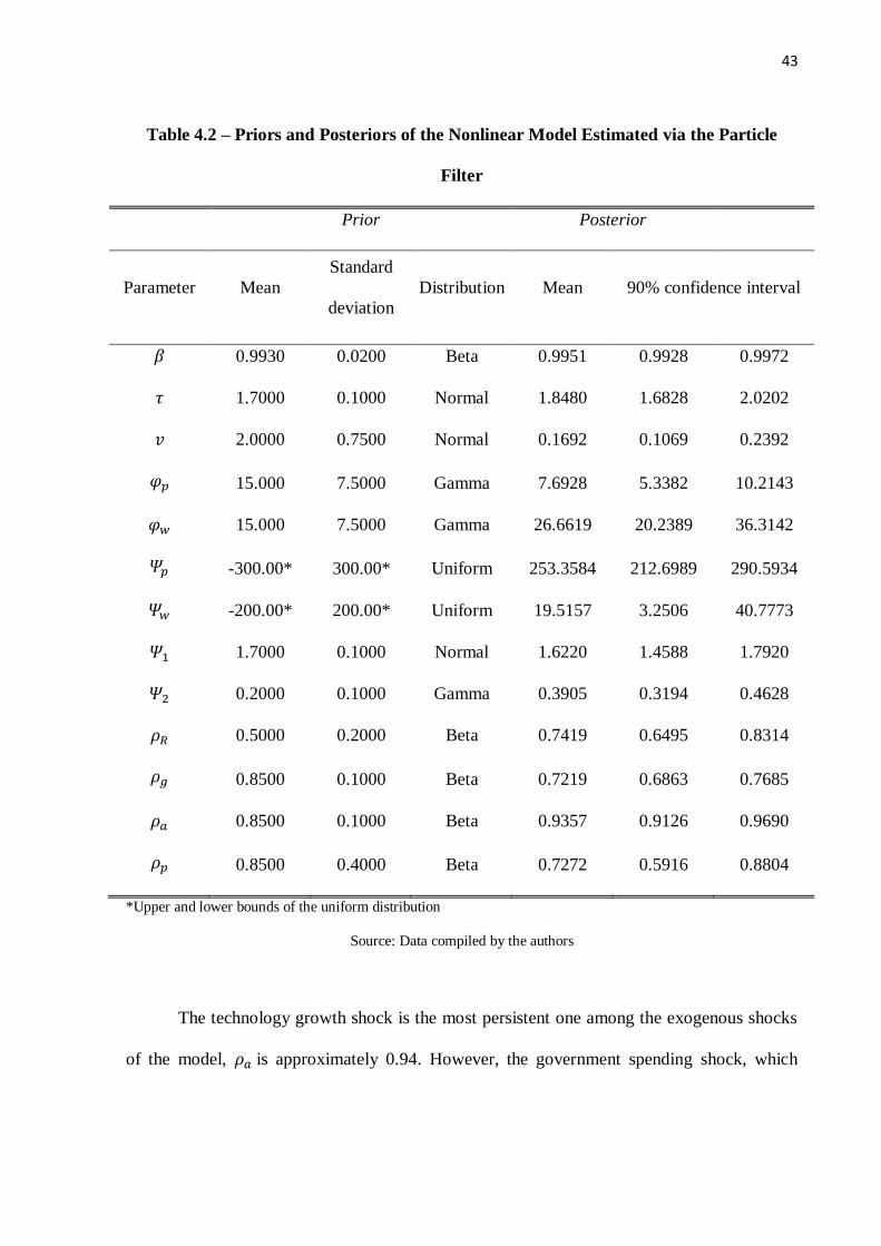
Table 4.2 – Priors and Posteriors of the Nonlinear Model Estimated via the Particle

Filter

Prior Posterior

Parameter Mean

Standard

deviation

Distribution Mean 90% confidence interval

𝛽 0.9930 0.0200 Beta 0.9951 0.9928 0.9972

𝜏 1.7000 0.1000 Normal 1.8480 1.6828 2.0202

𝑣 2.0000 0.7500 Normal 0.1692 0.1069 0.2392

𝜑𝑝 15.000 7.5000 Gamma 7.6928 5.3382 10.2143

𝜑𝑤 15.000 7.5000 Gamma 26.6619 20.2389 36.3142

𝛹𝑝 -300.00* 300.00* Uniform 253.3584 212.6989 290.5934

𝛹𝑤 -200.00* 200.00* Uniform 19.5157 3.2506 40.7773

𝛹1 1.7000 0.1000 Normal 1.6220 1.4588 1.7920

𝛹2 0.2000 0.1000 Gamma 0.3905 0.3194 0.4628

𝜌𝑅 0.5000 0.2000 Beta 0.7419 0.6495 0.8314

𝜌𝑔 0.8500 0.1000 Beta 0.7219 0.6863 0.7685

𝜌𝑎 0.8500 0.1000 Beta 0.9357 0.9126 0.9690

𝜌𝑝 0.8500 0.4000 Beta 0.7272 0.5916 0.8804

*Upper and lower bounds of the uniform distribution

Source: Data compiled by the authors

The technology growth shock is the most persistent one among the exogenous shocks

of the model, 𝜌𝑎 is approximately 0.94. However, the government spending shock, which

44

represents a generic demand shock, is given by 𝜌𝑔 = 0.7219. Finally, the persistence of the

shock to the inverse elasticity of demand for intermediate goods, 𝜌𝑝, is equal to 0.73.

Finally, the rigidity and asymmetry parameters are analyzed in the price and wage

adjustment cost functions. The parameters that govern price and wage rigidity, 𝜑𝑝 =

7.6928 and 𝜑𝑤 = 26.6619, indicate both price and wage rigidity in the Brazilian economy.

Moreover, the parameters show that wage rigidity is higher than price rigidity.

Notwithstanding, this finding can be explained by the values obtained for other rigidity

parameters – those which provide evidence of asymmetric rigidity – which will be discussed

in what follows. Therefore, the most interesting and important results are those related to

asymmetry parameters for price and wage adjustment cost functions, as these parameters have

not been estimated for the Brazilian economy yet. For parameters 𝛹𝑝 and 𝛹𝑤 the estimates

were 253.3584 and 19.5157, respectively. By comparing these results with those obtained by

Aruoba, Bocola & Shorfheide (2013), one has a higher value for asymmetric price (𝛹𝑝 =

165) and a lower one than that observed for asymmetric wage (𝛹𝑤 = 59). Also, by

comparing the findings with those described by Kim & Ruge-Murcia (2009), the wage

parameter is way below the values obtained by other authors (𝛹𝑤 = 901.4); however, in that

study, only wage asymmetry is assumed to exist, which might have influenced the results, in

addition to the fact that the authors estimated their DSGE model using the method of

simulated moments. By and large, the positive estimates of 𝛹𝑝 = 253.3584 and 𝛹𝑤 =

19.5157 imply that it is harder to lower prices and wages than to raise them; in addition, price

asymmetry is more pronounced than wage asymmetry. This result may have influenced the

value of parameters 𝜑𝑝 and 𝜑𝑤 mentioned earlier. Note that the value of 𝜑𝑝 was much lower

than 𝜑𝑤; on the other hand, the value of 𝛹𝑝 was much higher than 𝛹𝑤. What this result shows

is that the firm has a real cost (e.g., in terms of goods or hours worked) when it changes its

price, which is identified by parameter 𝜑𝑝, but because of the small value of this parameter,

45

the firms start with a low cost and then bring it closer to market efficiency when they adjust

their prices. Nevertheless, the high value of 𝛹𝑝 tells us that firms adjust their prices at a higher

cost when they need to lower rather than to increase their prices. The opposite is true for

wages, i.e., wage rigidity is high, but wage asymmetry is low although it indicates that the

cost associated with lowering them is higher. Thus, we gathered evidence that both prices and

wages are sticky in the Brazilian economy; furthermore, they are stickier downward than

upward. This may be so mainly due to the following factors. In the case of wages, as pointed

out by Camargo (2009), the Brazilian labor market has some peculiarities, with a

comprehensive body of laws governing its operation, in addition to being complex and giving

meticulous attention to detail, which eventually hinders the appropriate “drafting” of labor

contracts, with different characteristics from those established by law, rendering the labor

contract framework legally binding and barely negotiable. Hence, by drawing up contracts

with more flexible clauses than those required by law, firms risk having these contracts

declared void by the labor court, resulting in high costs. Therefore, wages become sticky. On

the other hand, the presence of strong unions in the domestic economy may produce

downward wage rigidity, more often than not, not allowing for cuts in wages based on

workers’ productivity. In the case of prices, two factors could explain rigidity. The first one

stems from wage rigidity itself, which ends up having an impact on firms’ costs. Since wages

are stickier downward, firms eventually do not adjust their prices efficiently (setting wages

according to productivity). Moreover, as highlighted previously, firms risk having to cover

high costs by trying to negotiate contracts that are more flexible than what the Brazilian law

stipulates, and are at risk of having these contracts deemed void, giving rise to expensive

lawsuits. The second situation is concerned with the fact that firms often operate in a market

that is not fully competitive, i.e., most firms have some monopoly over their products since

such products are minimally different from those marketed by their competitors. However, in

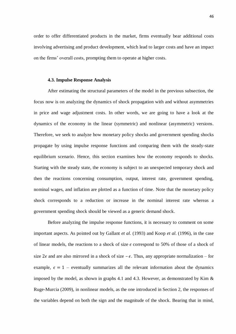
46

order to offer differentiated products in the market, firms eventually bear additional costs

involving advertising and product development, which lead to larger costs and have an impact

on the firms’ overall costs, prompting them to operate at higher costs.

4.3. Impulse Response Analysis

After estimating the structural parameters of the model in the previous subsection, the

focus now is on analyzing the dynamics of shock propagation with and without asymmetries

in price and wage adjustment costs. In other words, we are going to have a look at the

dynamics of the economy in the linear (symmetric) and nonlinear (asymmetric) versions.

Therefore, we seek to analyze how monetary policy shocks and government spending shocks

propagate by using impulse response functions and comparing them with the steady-state

equilibrium scenario. Hence, this section examines how the economy responds to shocks.

Starting with the steady state, the economy is subject to an unexpected temporary shock and

then the reactions concerning consumption, output, interest rate, government spending,

nominal wages, and inflation are plotted as a function of time. Note that the monetary policy

shock corresponds to a reduction or increase in the nominal interest rate whereas a

government spending shock should be viewed as a generic demand shock.

Before analyzing the impulse response functions, it is necessary to comment on some

important aspects. As pointed out by Gallant et al. (1993) and Koop et al. (1996), in the case

of linear models, the reactions to a shock of size 𝜖 correspond to 50% of those of a shock of

size 2𝜖 and are also mirrored in a shock of size – 𝜖. Thus, any appropriate normalization – for

example, 𝜖 = 1 – eventually summarizes all the relevant information about the dynamics

imposed by the model, as shown in graphs 4.1 and 4.3. However, as demonstrated by Kim &

Ruge-Murcia (2009), in nonlinear models, as the one introduced in Section 2, the responses of

the variables depend on both the sign and the magnitude of the shock. Bearing that in mind,

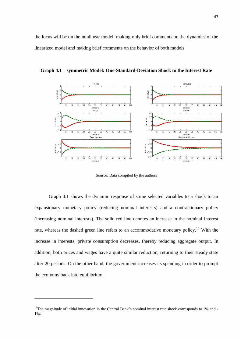
47

the focus will be on the nonlinear model, making only brief comments on the dynamics of the

linearized model and making brief comments on the behavior of both models.

Graph 4.1 – symmetric Model: One-Standard-Deviation Shock to the Interest Rate

Source: Data compiled by the authors

Graph 4.1 shows the dynamic response of some selected variables to a shock to an

expansionary monetary policy (reducing nominal interests) and a contractionary policy

(increasing nominal interests). The solid red line denotes an increase in the nominal interest

rate, whereas the dashed green line refers to an accommodative monetary policy.16

With the

increase in interests, private consumption decreases, thereby reducing aggregate output. In

addition, both prices and wages have a quite similar reduction, returning to their steady state

after 20 periods. On the other hand, the government increases its spending in order to prompt

the economy back into equilibrium.

16The magnitude of initial innovation in the Central Bank’s nominal interest rate shock corresponds to 1% and -

1%.

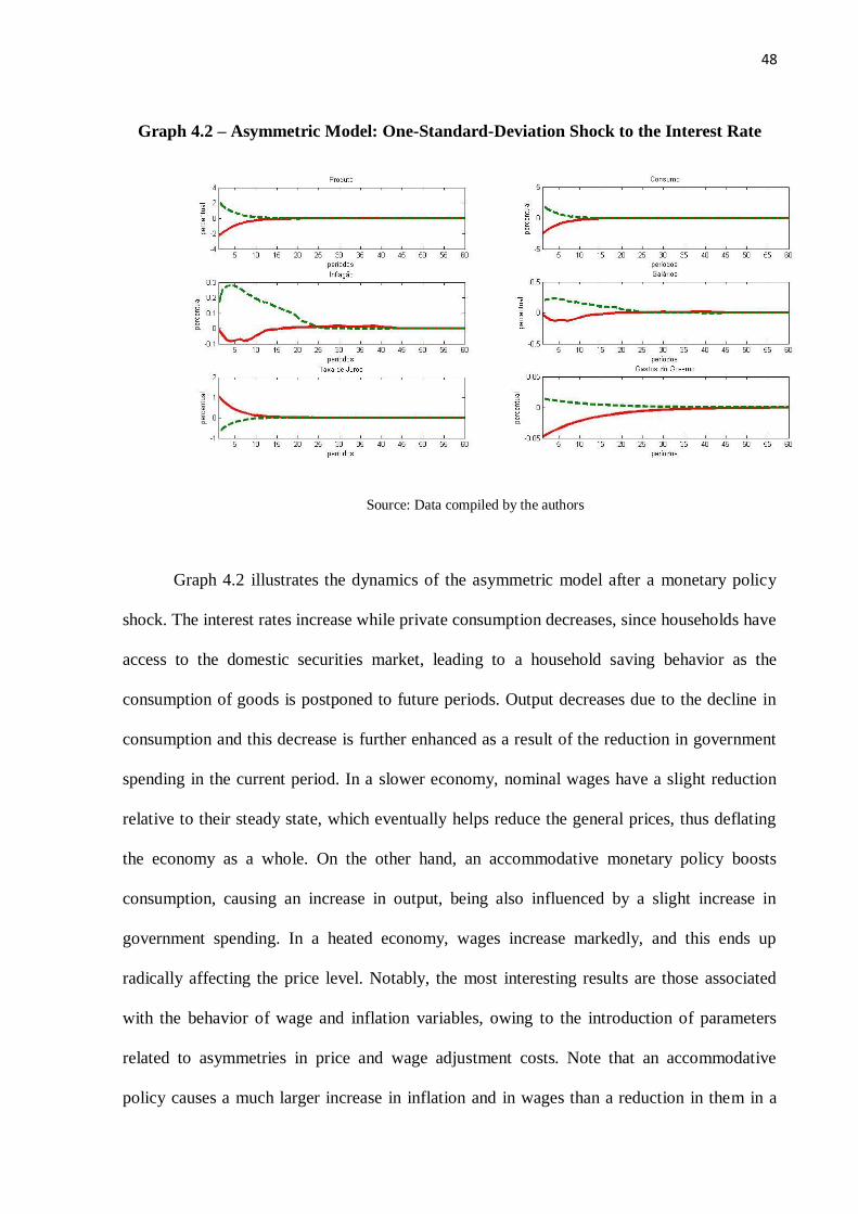
48

Graph 4.2 – Asymmetric Model: One-Standard-Deviation Shock to the Interest Rate

Source: Data compiled by the authors

Graph 4.2 illustrates the dynamics of the asymmetric model after a monetary policy

shock. The interest rates increase while private consumption decreases, since households have

access to the domestic securities market, leading to a household saving behavior as the

consumption of goods is postponed to future periods. Output decreases due to the decline in

consumption and this decrease is further enhanced as a result of the reduction in government

spending in the current period. In a slower economy, nominal wages have a slight reduction

relative to their steady state, which eventually helps reduce the general prices, thus deflating

the economy as a whole. On the other hand, an accommodative monetary policy boosts

consumption, causing an increase in output, being also influenced by a slight increase in

government spending. In a heated economy, wages increase markedly, and this ends up

radically affecting the price level. Notably, the most interesting results are those associated

with the behavior of wage and inflation variables, owing to the introduction of parameters

related to asymmetries in price and wage adjustment costs. Note that an accommodative

policy causes a much larger increase in inflation and in wages than a reduction in them in a

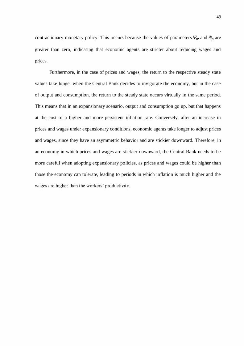
49

contractionary monetary policy. This occurs because the values of parameters 𝛹𝑤 and 𝛹𝑝 are

greater than zero, indicating that economic agents are stricter about reducing wages and

prices.

Furthermore, in the case of prices and wages, the return to the respective steady state

values take longer when the Central Bank decides to invigorate the economy, but in the case

of output and consumption, the return to the steady state occurs virtually in the same period.

This means that in an expansionary scenario, output and consumption go up, but that happens

at the cost of a higher and more persistent inflation rate. Conversely, after an increase in

prices and wages under expansionary conditions, economic agents take longer to adjust prices

and wages, since they have an asymmetric behavior and are stickier downward. Therefore, in

an economy in which prices and wages are stickier downward, the Central Bank needs to be

more careful when adopting expansionary policies, as prices and wages could be higher than

those the economy can tolerate, leading to periods in which inflation is much higher and the

wages are higher than the workers’ productivity.

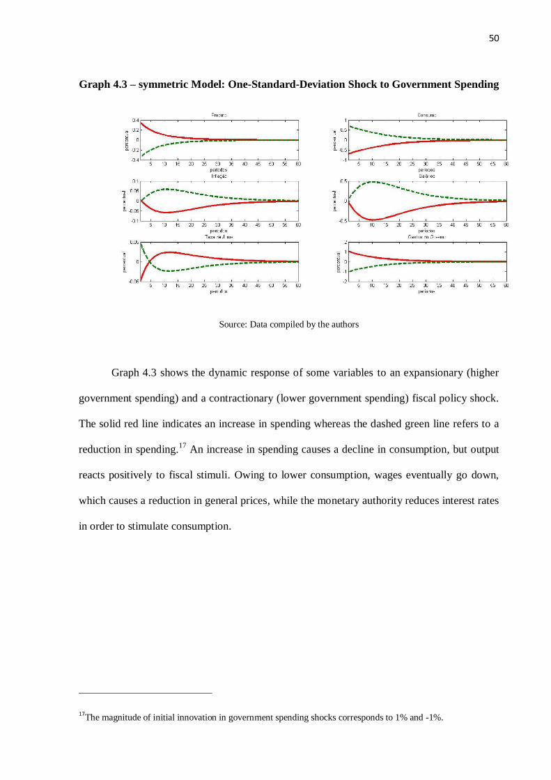
50

Graph 4.3 – symmetric Model: One-Standard-Deviation Shock to Government Spending

Source: Data compiled by the authors

Graph 4.3 shows the dynamic response of some variables to an expansionary (higher

government spending) and a contractionary (lower government spending) fiscal policy shock.

The solid red line indicates an increase in spending whereas the dashed green line refers to a

reduction in spending.17

An increase in spending causes a decline in consumption, but output

reacts positively to fiscal stimuli. Owing to lower consumption, wages eventually go down,

which causes a reduction in general prices, while the monetary authority reduces interest rates

in order to stimulate consumption.

17The magnitude of initial innovation in government spending shocks corresponds to 1% and -1%.

51

Graph 4.4 – Asymmetric Model: One-Standard-Deviation Shock to Government

Spending

Source: Data compiled by the authors

In Graph 4.4, when spending increases, private consumption decreases considerably,

since households in this economy are Ricardian; consequently, there is a large crowding out

effect, in which an increase in government spending reduces private consumption. Output

increases slightly in the first quarters even with the abrupt reduction in household

consumption, but it goes back quickly to the initial steady state. This increase can be

explained by a boost in demand caused by higher government spending. Regarding nominal

wages, they are increased slightly as a result of the initial fiscal incentive. Nonetheless, as

private consumption declines and aggregate output returns to its steady state rather quickly,

wages go back to a lower level in subsequent quarters. The increase in wages eventually

affects inflation and thus the Central Bank intervenes by driving interests up in order to

counteract the inflationary effects in the short run. On the other hand, a contractionary fiscal

policy brings about a small increase in household consumption whereas aggregate output

shows a remarkable reduction. Due to burgeoning demand, resulting from an increase in

52

private consumption, nominal wages go up sharply and remain way above the point of

equilibrium for a long time. With higher wages, firms opt to increase the prices of their

products so as to adjust to household income, thus maximizing their profit, at least in the short

run. As shown in Graph 4.4, wage and price movements are similar, indicating downward

rigidity, caused by the introduction of asymmetric adjustment costs in the model. When an

inflationary period is observed, the monetary authority increases the interest rates; however,

the increase in interest rates is smaller than the previous one. Apparently, the Central Bank

decides to fight inflationary effects, but as aggregate output decreases, the increase in interest

rates does not take place abruptly so as not to push aggregate output further down. This

behavior is quite similar to that observed in the past four years, in which the Central Bank was

more tolerant of inflation to prevent output from being affected by higher interest rates. In

summary, as shown in Graph 4.4, fiscal expansion contributes little to aggregate output

movement whereas fiscal contraction causes a decrease in output. The effects on wages and

on inflation may be severe both in an expansionary and contractionary policy environment.

Finally, by comparing the behavior of the symmetric model with that of the

asymmetric one, when there is a monetary policy shock, an expansionary policy causes a

similar wage movement in both models. However, prices increase more abruptly in the

asymmetric model and stay off the equilibrium path for a longer time (around five quarters

more than in the linearized model), indicating higher persistence of inflationary effects on the

Brazilian economy when the agents behave asymmetrically towards prices and wages. In the

case of consumption and output, the responses are very similar in both models, showing that

nonlinearities in prices and wages do not drastically affect the behavior of these variables. On

the other hand, in the presence of a fiscal policy shock, output and consumption behave

differently in each model. In the case of prices and wages, a temporary fiscal imbalance

eventually leads to higher disequilibrium in both models, taking around 55 periods to return to

53

the steady state, five quarters more than in the asymmetric model. In brief, the comparison of

the dynamics of both models in the presence of a monetary or fiscal policy shock shows a

much larger effect on prices and wages in the asymmetric case. This finding was expected

since the estimated parameters associated with the level of asymmetry in the nonlinear model

provide evidence that the economy is stickier downward. Accordingly, in an economy in

which price and wage setters are stickier downward, both the Central Bank and the fiscal

authority should proceed with caution, as an accommodative policy or an imbalance in public

accounts eventually has a stronger impact on wages and on inflation and, consequently, the

economy will need a longer time to adjust. Thus, at election time, when the incumbent

government often creates economic incentives, an imbalance in public accounts or a reduction

in interest rates by the Central Bank in order to boost credit and consumption can lead to

higher and more persistent inflation rates, preventing the economy from returning as fast as

possible to its steady state.

5. Conclusion

The use of linearized DSGE models turned the Kalman filter into the standard tool for

likelihood estimation, helping with the estimation of these economic models. However, this

filter often has a very restrictive framework, thus limiting the analysis of nonlinear

phenomena observed in the real world. Therefore, the pioneering work by Fernández-

Villaverde & Rubio-Ramírez (2005) opened up a new avenue to the study of nonlinear

macroeconomic models by developing a sequential Monte Carlo algorithm that allows

estimating the likelihood function of a model solved by a nonlinear method. From then on,

several studies on the estimation of nonlinear models with the use of sequential Monte Carlo

methods have been conducted, including, among others, An & Schorfheide (2007),

54

Fernández-Villaverde & Rubio-Ramírez (2007), Amisano & Tristani (2010), Andreasen

(2011), and Fasolo (2012).

Among these methods, the particle filter is the most famous one. It is a numerical state

estimator that is fully nonlinear and that can be used to estimate any model in state-space

form. According to Simon (2006), the particle filter, or Monte Carlo filter, is a “brute force”

statistical method that often works well with problems that are not easily solved by the

conventional Kalman filter, i.e., highly nonlinear systems.

Thus, having at hand a statistical tool that allows using nonlinear DSGE models,

which generates a better representation of the economy, it is possible to use a model that

generates fundamental nonlinearities. Taking this into consideration, a DSGE model with

asymmetric price and wage adjustment costs, proposed by Kim & Ruge-Murcia (2009) and

expanded by Aruoba, Bocola & Shorfheide (2013), was used, producing nonlinearity in the

economic agents’ behavior. This model allows checking whether prices and wages are stickier

upward or downward. In other words, the aim of this paper was to verify whether price and

wage rigidity in the Brazilian economy is asymmetric and how it affects the dynamics of the

economy. Therefore, the present study estimated the structural parameters of the Brazilian

economy and assessed the behavior of the major macroeconomic variables towards monetary

and fiscal policy movements. The model is solved by using second-order perturbation

methods based on Schmitt-Grohé & Uribe (2004) and estimated with Brazilian data, using the

particle filter in order to construct the likelihood.

The results provide evidence that wages and prices in the Brazilian economy are

stickier downward, as the parameters associated with asymmetric rigidity are greater than

zero. In other words, there is asymmetry – which is weaker in the case of wages and stronger

in the case of prices – making economic agents be stricter when it comes to reducing rather

than increasing wages and prices. These asymmetries, in the case of prices, may be caused by

55

some monopoly on the part of firms or result from the downward wage rigidity, since most of

the costs defrayed by firms are associated with their payrolls. Asymmetry in wages may be

attributed to the characteristics of the Brazilian labor market, due to a very complex body of

laws governing the drafting of contracts. Moreover, there is high turnover and a large number

of informal job contracts, which may result in remarkable asymmetries.

Based on the impulse response analysis, it is possible to conclude that in the presence

of asymmetries in price and wage rigidity, the Central Bank should be more careful about the

formulation of an expansionary monetary policy, given that prices and wages are stickier

downward and monetary easing could thus lead to longer periods of high inflation. Likewise,

fiscal policy movements (be they expansionary or contractionary) eventually have a negative

impact, especially on inflation, which means that it is better to keep the fiscal policy in its

steady state, i.e., to have a neutral fiscal policy. Additionally, by comparing the dynamics of

asymmetric economy (solved by a nonlinear method and estimated by a particle filter) with

symmetric economy (linearized version in which likelihood is estimated by the Kalman filter),

it was observed that nonlinear economy takes longer to return to its steady state after a

monetary or fiscal shock and that nonlinearities are more pronounced in prices and wages

than in any other macroeconomic variables.

Finally, several elements can be added and improved in a future study. It would be

interesting, for instance, to investigate the underlying causes of asymmetries in price and

wage rigidity. In addition, another suggestion is to use a DSGE model for an open economy

and include capital accumulation in order to bring the theoretical model as closest as possible

to the real economy. Regarding the particle filter, it would be interesting to use extensions of

this filter, such as the conditional particle filter (Amisano & Tristani, 2010) or the particle

filter proposed by Andreasen (2011) in an attempt to further improve its estimates.

56

References

ALVES, S. A. L. Essays on Trend Inflation: Optimal Policy, Estimation Bias, and

Unemployment Volatility. PhD Thesis, University of California, Santa Cruz, October, 2011.

AMISANO, G.; TRISTANI, O. Euro Area Inflation Persistence in an Estimated Nonlinear

DSGE Model. Journal of Economic Dynamics & Control. 34, p. 1837-1858, 2010.

AN, S. Bayesian Estimation of DSGE Models: Lessons from Second-Order

Approximations, 2007.

AN, S.; SCHORFHEIDE, F. Bayesian Analysis of DSGE Models. Econometric Review, n.

26, p. 187-192, 2007.

ANDREASEN, M. M. Non-Linear DSGE Models and the Optimized Central Difference

Particle Filter. Journal of Economic Dynamics and Control, v. 35, n. 10, p. 1671-1695,

2011.

ARUOBA, S. B.; BOCOLA, L.; SCHORFHEIDE, F. Assessing DSGE Model

Nonlinearities. Manuscript, University of Pennsylvania, 2013.

ARUOBA, S. B.; FERNÁNDEZ-VILLAVERDE, J. F.; RUBIO-RAMÍREZ, R. J. Comparing

Solution Methods for Dynamic Equilibrium Economies. Journal of Economic Dynamic and

Control, 30 (12), p. 2477-2508, 2006.

BERGER, J. O.; WOLPER, R. L. The Likelihood Principle. Institute of Mathematical

Statistics, Lecture Notes Volume 6. 1988.

CALVO, G. Staggered Prices in a Utility Maximizing Framework. Journal of Monetary

Economics. V. 12, p. 383-398, 1983.

CAMARGO, J. M. Desemprego, Informalidade e Rotatividade: Reformas que Fazem

Diferença. Em: GIAMBIAGI, F.; BARROS, O. (Orgs.). Brasil Pós-Crise: Agenda para a

Próxima Década. Rio de Janeiro, Elsevier, 2009. Parte II, Cap. 14, p. 231-244.

CASTRO, M. R. et al. Samba: Stochastic Analytical Model with a Bayesian Approach.

Banco Central do Brasil, Working Paper Series, n. 239. Brasília: BCB, 2011.

CHIB, S. Markov Chain Monte Carlo Methods: Computational an Inference, In: HECKMAN,

J. J.; LEAMER, E. Handbook of Econometrics. Amsterdam: Elsevier Science, 2001. Vol. 5,

Cap. 57, p. 3569-3649.

CHRISTIANO, L. J.; EICHENBAUM, M.; EVANS, C. L. Monetary Policy Shocks: What

Have We Learned and What End? In: TAYLOR, J. B.; WOODFORD, M.; Handbook of

Macroeconomics 1A. Amsterdam: Elsevier Science, p. 65-148, 1999.

CHRISTIANO, L. J.; EICHENBAUM, M.; EVANS, C. L. Nominal Rigidities and the

Dynamic Effects of a Shock to Monetary Policy. Journal of Political Economy.113, p. 1-45,

2005.

57

COX, I. J. Blanche – An Experiment in Guidance and Navigation of an Autonomous Robot

Vehicle. IEEE Transactions on Robotics and Automation, v. 7, n. 2, p. 193-204, abr.,

1991.

DEJONG, D. N.; DAVE, C. Structural Macroeconometrics. Princeton, NJ: Princeton

University Press; 2007.

DEJONG, D. N. el al. Efficient Likelihood Evaluation of State-Space Representations.

Czech National Bank, Working Papers, 2009.

FASOLO, A. M. A Note on Particle Filter Applied to DSGE Models. Banco Central

Working Papers Series 281, Banco Central do Brasil, 2012.

FERNÁNDEZ-VILLAVERDE, J. F; RUBIO-RAMÍREZ, R. J. Estimating Dynamic

Equilibrium Economies: Linear Versus Nonlinear Likelihood. Journal of Applied

Econometrics, 20 (7): 891-910. 2005.

FERNÁNDEZ-VILLAVERDE, J. F; RUBIO-RAMÍREZ, R. J. Estimating Macroeconomic

Model: A Likelihood Approach. Mimeo, University of Pennsylvania. 2007.

FERNÁNDEZ-VILLAVERDE, J. F; RUBIO-RAMÍREZ, R. J.; SANTOS, M. S.

Convergence Properties of the Likelihood of Computed Dynamic Models. Econometrica, 74

(1): 93-119. 2006.

FLURY, T.; SHEPHARD, N. Bayesian Inference Based Only on Simulated Likelihood:

Particle Filter Analysis of Dynamic Economic Models. Econometric Theory, 27 (5), p. 933-

956, 2011.

GALÍ, J. Monetary Policy, Inflation and the Business Cycle: An Introduction to the New

Keynesian Framework. Princeton and Oxford, 2008.

GALLANT, A. R.; ROSSI, P. E.; TAUCHEN, G. Nonlinear Dynamic Structures.

Econometrica, 61, p. 871-908, 1993.

GIAMBIAGI, F.; VILLELA, A. (Orgs.). Economia Brasileira Contemporânea (1954-

2004). Rio de Janeiro, Elsevier, 2005.

GOMME, P.; KLEIN, P. Second-Order Approximation of Dynamic Models Without the

Use of Tensors. Mimeo, University of Western Ontario, 2008.

GORDON, N. J.; SALMOND, D. J.; SMITH, A. F. M. Novel approach of Nonlinear/Non-

gaussian Bayesian State estimation. Radar and Signal Processing, IEE Proceedings-F, 140

(2), 107-113, 1993.

JUDD, K. L. Numerical Methods in Economics. Cambridge, Massachussets: MIT Press,

1998.

JUDD, K. L.; GUU, S. M. Asymptotic Methods for Aggregate Growth Models. Journal of

Economic Dynamic and Control, 21 (6), p. 1025-1042, 1997.

58

KALMAN, R. E. A New Approach to Linear Filtering and Linear Problems. Transaction of

the ASME – Journal of Basic Engineering, 82 (Series D): 35-45. 15. 1960.

KIM, J.; F. RUGE-MURCIA. How Much Inflation is Necessary to Grease the Wheels.

Journal of Monetary Economics, n. 56, p. 365-377, 2009.

KIM, J.; KIM, S.; SCHAUMBURG, E. SIMS, C. Calculating and Using Second Order

Accurate Solutions of Discrete Time Dynamic Equilibrium Models. Mimeo, 2003.

KIM, S.; SHEPHARD, N.; CHIB, S. Stochastic Volatility: Likelihood Inference and

Comparison with Arch Models. Review of Economic Studies, 65 (3), p. 361-93, 1998.

KITAGAWA, G. Non-gaussian State Space Modeling of Nonstationary Time Series. Journal

of the American Statistical Association, 82 (400): 1032-1041. 15, 22. (1987).

KITAGAWA, G. Monte Carlo Filter and Smoother for non-gaussian nonlinear state space

models. Journal of Computational and Graphical Statistics, 5 (1): 1-25.105, 109, 110.

(1996).

KOOP, G.; PESARAN, M. H.; POTTER, S. Impulse Response Analysis in Non-linear

Multivariate Models. Journal of Econometrics, 74, p. 119-147, 1996.

KYDLAND, F.; PRESCOTT, E. Time to Build and Aggregate Fluctuations. Econometrica,

v. 50, p. 1345-1370, 1982.

LUCAS, R. E. Jr. Econometric Policy Evaluation: A Critique. Carnegie-Rochester

Conference Series on Public Policy, v. 1, p. 19-46, 1976.

LUCAS, R. E. Jr.; PRESCOTT, E. C. Investment under Uncertainty. Econometrica, n. 39, p.

659-681, 1971.

METROPOLIS, N.; ULAM, S. The Monte Carlo Method. Journal of the American

Statistical Association, v. 44, n. 247, p. 335-341, 1949.

MIRANDA, M. J.; FACKLER, P. L. Applied Computational Economics and Finance. The

MIT Press, 2002.

MONFORT, A. A Reappraisal of Misspecified Econometric Models. Econometric Theory

12, 597-612. 1996.

MOURA, G. V. Efficient Importance Sampling in Applied Econometrics. PhD thesis,

Christian- Albrechts-Universität Zu Kiel, C.A.U., Germany, 2010.

PITT, M. K.; SHEPHARD, N. Filtering via Simulation: Auxiliary Particle Filters. Journal of

the American Statistical Association, 94 (446), p. 590-559.

PORTUGAL, M.; SILVA, F. O Impacto de Choques Fiscais na Economia Brasileira:

Uma Abordagem DSGE. Texto para Discussão do Programa de Pós-Graduação em

Economia da UFRGS. 2011.

59

REBELO, S. Real Business Cycle Models: Past, Present, and Future. Northwestern

University, March, 2005.

ROMER, D. Advanced Macroeconomics. New York, McGraw-Hill/Irwin, 4th Edition,

2012.

ROTEMBERG, J. Monopolistic Price Adjustment and Aggregate Output. Review of

Economic Studies, n. 49, p. 517-531, 1982.

SANTOS, F. G.; KANCZUK, F. Price Puzzle e Canal de Custo da Política Monetária:

Evidência para a Economia Brasileira. ANPEC, 2011.

SCHMITT-GROHÉ, S.; URIBE, M. Optimal Fiscal and Monetary Policy under Stick Prices.

Journal of Economic Theory, n. 114, p. 198-230, 2004.

SCHMITT-GROHÉ, S.; URIBE, M. Solving Dynamic General Equilibrium Models Using a

Second-Order Approximation to the Policy Function. Journal of Economic Dynamic and

Control, n. 28, p. 755-775, 2004.

SCHORFHEIDE, F. Loss Function-Based Evaluation of DSGE Models. Journal of Applied

Econometrics, n. 15, p. 645-670, 2000.

SIN, H.; GAGLIANONE, W. Stochastic Simulation of a DSGE Model for Brazil, MPRA, n.

20853, 2006.

SMITH, A.; GELFAND, A. Bayesian Statistics without Tears: A Sampling-Resampling

Perspective. The American Statistician, 46 (2), p. 84-88, 1992.

SIMON, D. Optimal State Estimation: Kalman, 𝒉∞, and Nonlinear Approaches.

Hoboken: John Wiley, 2006.

SIMS, C. Macroeconomics and Reality. Econometrica, v. 48, n. 1, p. 1-48, 1980.

SIMS, C. Solving Linear Rational Expectations Models. Computational Economics, v. 20,

p. 1-20, 2001.

SMETS, F.; WOUTERS, R. An Estimated Stochastic Dynamic General Equilibrium Model of

the Euro Area. Journal of the European Economic Association, v.1, p. 1123-1175, 2004.

STRID, I. Parallel Particle Filters for Likelihood Evaluation in DSGE Models: As

Assessment. In: Proceeding of the Computing in Economics and Finance. Society for

Computational Economics, v. 395, 2006.

VASCONCELOS, B.; DIVINO, J. O Desempenho Recente da Política Monetária Brasileira

sob a Ótica da Modelagem DSGE. Trabalhos para Discussão do Banco Central do Brasil,

n. 291, 2012.

VARIAN, H. A Bayesian Approach to Real Estate Assessment. In: FEINBERG, S. E.;

ZELLNER, A. Studies in Bayesian Economics in Honor of L. J. Savage. Amsterdam:

North-Holland, 1974.