Firm Heterogeneity and Export Pricing in India

Michael A. AndersonWashington and Lee University

Martin H. DaviesWashington and Lee University

Center for Applied Macroeconomic Analysis, Australia National University

Jose E. SignoretU.S. International Trade Commission

Stephen L. S. SmithGordon College

The views in this presentation are strictly those of the authors and do not represent the opinions of the U.S. International Trade Commission or any of its individual Commissioners.

Plan• motivation and contribution• literature review: theory and empirics• data• results• discussion• conclusion

Motivation and Contribution

• New dataset (Prowess + TIPS) that allows us to examine pricing behavior of Indian exporters

• Motivation: Indian firms: the same or different?

• Previous studies, for a number of countries, find:• more productive firms charge higher prices,• prices rise with distance and fall with remoteness.

• By contrast we find Indian firms are different:• more productive firms charge lower prices,• prices fall with distance and rise with remoteness.

• What are Indian firms doing differently?

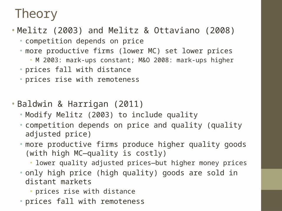
Theory• Melitz (2003) and Melitz & Ottaviano (2008)• competition depends on price• more productive firms (lower MC) set lower prices

• M 2003: mark-ups constant; M&O 2008: mark-ups higher• prices fall with distance • prices rise with remoteness

• Baldwin & Harrigan (2011)• Modify Melitz (2003) to include quality• competition depends on price and quality (quality adjusted price)• more productive firms produce higher quality goods (with high MC

—quality is costly)• lower quality adjusted prices—but higher money prices

• only high price (high quality) goods are sold in distant markets• prices rise with distance

• prices fall with remoteness

Literature• heterogeneous goods, heterogeneous markets• China: Manova and Zhang (2012)• Colombia: Kugler and Verhoogen (2012)• US: Harrigan, Ma, and Shlykov (2015)• Portugal: Bastos and Silva (2010)• Hungary: Gorg, Halpern, and Murakozy (2010)• France: Martin (2009)

• Findings:• Firms price discriminate across destinations • Higher productivity firms charge higher prices

• linked to product quality upgrades.• prices increase with distance: all papers• prices fall with remoteness: MZ, HMS• above are consistent with Baldwin & Harrigan quality-adjusted Melitz

(2003)

Theory: Antoniades (2015)• heterogeneous markets: quality ladders long

• correlation between prices and productivity positive• homogeneous market: quality ladders short

• correlation between prices and productivity negative

• Sign of relationship depends on scope for quality differentiations (cost of quality upgrading): determined by• market size (L), • the degree of differentiation between varieties (1/γ)• cost of innovation (θ)• appreciation of quality (β)

then > 0 scope for quality differentiation is low then < 0 scope for quality differentiation is high

where 1/c is productivity and δ measures the cost of quality upgrading

• homogeneous goods: γ → ∞, and → 0 .

Diagram: Scope for quality differentiation

Scope for quality differentiation: low Scope for quality differentiation: high

CORRELATION BETWEEN PRICES AND PRODUCTIVITYSimple example

• two firms: high productivity (H) and low productivity (L)• marginal cost firm i: ci mark-up firm i: μi

cL > cH → μL < μH

• price = mc + mark-up pi = ci + μi

Two Cases:• scope for quality differentiation: high

pH = cH + μH > pL = cL + μL

HIGH PRODUCTIVITY FIRM HAS HIGHER PRICE

• scope for quality differentiation: lowpH = cH + μH < pL = cL + μL

LOW PRODUCTIVITY FIRM HAS HIGHER PRICE

Literature• heterogeneous goods, heterogeneous markets• China: Manova and Zhang (2012)• Columbia: Kugler and Verhoogen (2012)• US: Harrigan, Ma, and Shlykov (2015)• Portugal: Bastos and Silva (2010)• Hungary: Gorg, Halpern, and Murakozy (2010)• France: Martin (2009)

• Findings:• Firms price discriminate across destinations • Higher productivity firms charge higher prices

• linked to product quality upgrades.• prices increase with distance: all papers• prices fall with remoteness: MZ, HMS• above are consistent with Baldwin & Harrigan quality-adjusted Melitz

(2003)

Literature

• homogeneous goods, homogeneous markets• Roberts and Supina: (1996, 2000): white pan bread, coffee, tin cans,

corrugated boxes, gasoline, concrete• Syverson (2007): ready-mix concrete• Foster, Haltiwanger, Syversion (2008): ice, concrete, sugar, boxes,

oak flooring

• Findings• prices fall with productivity

• heterogeneous goods, homogeneous markets• this paper

III. Data

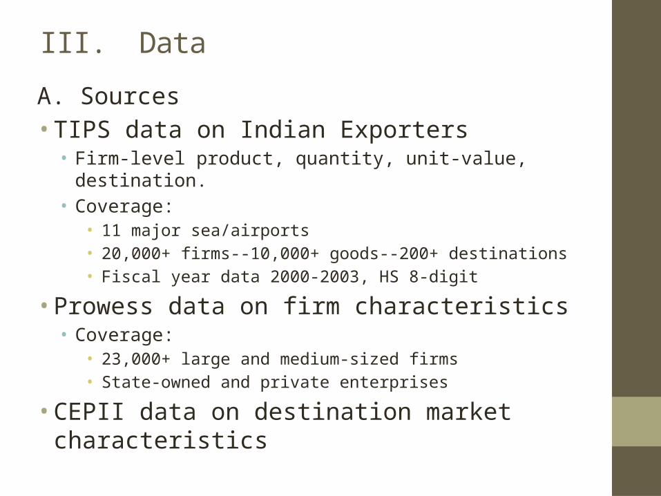
A. Sources• TIPS data on Indian Exporters

• Firm-level product, quantity, unit-value, destination.• Coverage:

• 11 major sea/airports• 20,000+ firms--10,000+ goods--200+ destinations• Fiscal year data 2000-2003, HS 8-digit

• Prowess data on firm characteristics• Coverage:

• 23,000+ large and medium-sized firms• State-owned and private enterprises

• CEPII data on destination market characteristics

III. DataB. Construction• Aggregation issues• …over time• …over firm IDs• …over product IDs• …over units

C. Result• 20,850 observations of unique firm-product-unit value-

destination-year data• All matched with firm and destination characteristics• 1,018 unique manufacturing firms

• Overall export revenue rises: $143 million (2000) to $520 million (2003)• Exports dominated by a few firms: top 10 percent export 80

percent of value• Sources of revenue growth: • Pure extensive growth—new revenue from new products, new

destinations—accounts for 40-50 percent of revenue increases. • At least half is from intensive growth—ongoing sales of established

goods to established destinations.

IV. ResultsA. Descriptive findings

A. Descriptives (cont.)

• Intensive revenue growth can be decomposed into contributions of price and quantity changes

• Unconditioned finding: revenue growth occurs through quantity increases rather than price increases.

• n = 2,545 continuing firm-product-destination combinations for which rates of change can be calculated:• Median revenue change: 38.7%• Median price change: -1.0%• Median quantity change: 50.0%

Cross-tabulation of price, quantity changes

Table 5. B. Continuing Firm-Product Observations With Positive Revenue Growth (n = 1,532) Percent (number) %quantity

%price (-) (+) Total (-) 0 (0) 50.2 (770) 50.3 (770) (+) 4.7 (73) 44.9 (689) 49.7 (762)

Total 4.9 (73) 95.1 (1,459) 100.0 (1,532)

IV. Results (cont.)B. Conditioned results• Dependent variable: export unit value• Independent variables:• Country variables:

• GDP per capita (loggdppc)• GDP (loggdp)• Distance (logdist)• Remoteness (logremote)

• Product fixed effects• Firm variables:

• TFP (logtfp)—Levinsohn-Petrin on gross value added, indexed• K/L (logklabor)• Size, proxied by wagebill (loglabor)

Selection correction

• Bias because firms’ prices only observed if firms choose to export to particular destinations.

• HMS’s 3-stage estimator• Extension of Wooldridge (1995).• 1st stage:Probit of entry (firm in a destination) estimated over

all possible firm-destination-year combinations. • 2nd stage: OLS regression of (positive) firm-product-

destination revenue on inverse Mills ratio, export-market and firm

characteristics. • 3rd stage: OLS regression of firm unit values on partial

residualsfrom 2nd stage (actual residuals plus estimated term for the inverse Mills ratio), export-market and firm characteristics.

Table 5. Firm-Product Pricing by Destination and Firm Characteristics—With and Without Sample Selection Correction

All Goods

(1) (2) VARIABLES logprice logprice loggdppc 0.0892*** 0.177***

(0.0209) (0.0277) loggdp 0.0366*** 0.271***

(0.0133) (0.0540) logdist -0.0242 -0.373***

(0.0473) (0.0661) logremote 0.00446 0.361***

(0.0432) (0.0779) logtfp -0.171** -0.162**

(0.0827) (0.0816) logklabor 0.0823 0.0933*

(0.0554) (0.0560) loglabor 0.0645* 0.181***

(0.0345) (0.0334) selection 0.211***

(0.0464) Observations 20,850 20,850 R-squared 0.862 0.871 Fixed effects Prod Prod SE clusters Country Country Robust standard errors in parentheses *** p<0.01, ** p<0.05, * p<0.1

Table 5.B. Firm-Product Pricing by Destination and Firm Characteristics—With Sample Selection Correction

All goods

Textile and textile articles

Machinery, appliances,

elect. equipment

All other HS chapters

(2) (4) (6) (8) VARIABLES logprice logprice logprice logprice loggdppc 0.177*** 0.127*** 0.0136 0.163***

(0.0277) (0.0249) (0.0472) (0.0274) loggdp 0.271*** 0.189*** 0.194*** 0.230***

(0.0540) (0.0387) (0.0555) (0.0449) logdist -0.373*** -0.162** -0.330*** -0.300***

(0.0661) (0.0678) (0.112) (0.0586) logremote 0.361*** 0.240*** 0.347*** 0.244***

(0.0779) (0.0510) (0.126) (0.0701) logtfp -0.162** -0.137** -0.565*** -0.208**

(0.0816) (0.0688) (0.173) (0.0881) logklabor 0.0933* 0.0102 0.0258 0.158**

(0.0560) (0.0308) (0.183) (0.0754) loglabor 0.181*** 0.162*** 0.388*** 0.0973**

(0.0334) (0.0269) (0.105) (0.0394) selection 0.211*** 0.0355*** 0.269*** 0.242***

(0.0464) (0.00698) (0.0386) (0.0567) Observations 20,850 2,915 4,233 13,657 R-squared 0.871 0.919 0.913 0.842 Fixed effects Prod Prod Prod Prod SE clusters Country Country Country Country

Results: Main Findings…

VARIABLES(2)

logprice

loggdppc 0.177***(0.0277)

loggdp 0.271***(0.0540)

logdist -0.373***(0.0661)

logremote 0.361***(0.0779)

logtfp -0.162**(0.0816)

logklabor 0.0933*(0.0560)

loglabor 0.181***(0.0334)

Observations 20,850R-squared 0.871

• 1. Pricing-to-market• 2. Prices… • fall with firm productivity• fall with distance• rise with remoteness

• 3. Results unchanged with differentiated goods defined by Rauch categories.• 4. Prices rise with firm size

and K/L

Discussion:Three Zones: I, II, III

Discussion: three zones • Zone III: heterogeneous goods, heterogeneous markets• US, China, Portugal, Hungary, France, Columbia

• Zone I: homogeneous goods, homogeneous markets• white pan bread, coffee, tin cans, corrugated boxes, gasoline,

concrete

• Zone II: heterogeneous goods, homogeneous markets• this paper

Discussion: China v India: scope of q.d. 2000-2005

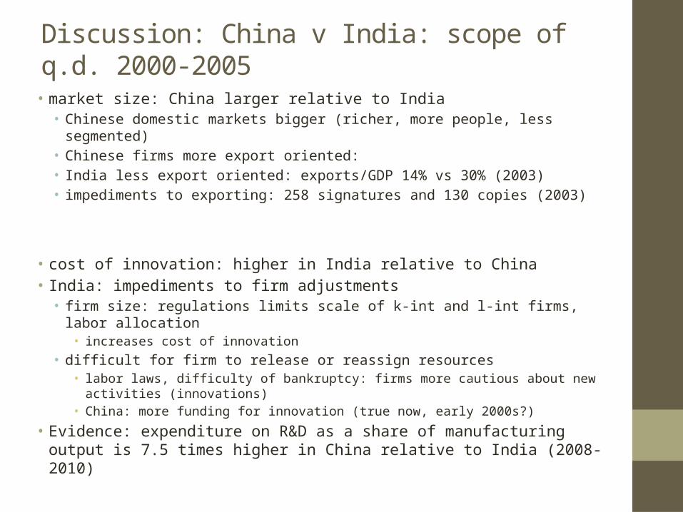
• market size: China larger relative to India• Chinese domestic markets bigger (richer, more people, less segmented)• Chinese firms more export oriented: • India less export oriented: exports/GDP 14% vs 30% (2003)• impediments to exporting: 258 signatures and 130 copies (2003)

• cost of innovation: higher in India relative to China• India: impediments to firm adjustments• firm size: regulations limits scale of k-int and l-int firms, labor allocation

• increases cost of innovation• difficult for firm to release or reassign resources

• labor laws, difficulty of bankruptcy: firms more cautious about new activities (innovations)

• China: more funding for innovation (true now, early 2000s?)

• Evidence: expenditure on R&D as a share of manufacturing output is 7.5 times higher in China relative to India (2008-2010)

Discussion: what is driving result• Divide observations along two lines:

1. by ternary Rauch Categories: homogeneous; reference-priced; differentiated

2. main groups in • Machinery (20%) – all differentiated• Textiles (14%) – 62% differentiated• All other goods (66%) – 57% differentiated

• Correlation (conditioned) strongest in machinery (all differentiated) (-0.53)• where expect correlation might positive it is most negative.

Remoteness, Distance

• heterogeneous markets (rest of literature)• prices and quality positively correlated• highest priced goods are highest quality and lowest price per unit of

quality => most competitive• distance: only highest priced goods make it to most distant markets

• price rises with distance• remoteness: only most competitive goods compete in areas with high

mass of economic activity• prices fall with remote

• homogeneous markets (this paper)• prices and quality negatively correlated• lowest prices goods has the lowest price per unknit of quality => most

competitive• distance: prices fall with distance• remoteness: prices rise with remoteness.

Conclusions• Indian firms are different• New empirical findings: • Indian firms with higher productivity charge lower prices in

destination markets• Negative association between distance and prices• prices increase with remoteness

• results: heterogeneous goods, homogeneous markets: Zone II• firms quality upgrading • but mark-ups rise too slowly to offset falling MC

• in contrast to:• heterogeneous goods, heterogeneous markets: Zone III• homogeneous goods, homogeneous markets: Zone I