Firm entry, product repositioning and welfare�

Eleftherios ZachariasAthens University of Economics and Bussiness,76 Patission Str., 104 34 Athens, GreeceRimini Centre for Economic Analysis

Email: ezachar@aueb.gr

May 7, 2009

Abstract

We show that the entry of a second �rm in a horizontally di¤erenti-ated market (ala Hotelling) may harm consumers as prices increase andconsumer�s surplus possibly decrease. We �rst derive the price and theconsumer�s surplus of a monopoly which is located at the center of themarket. When a second �rm enters the market the �rst �rm repositionsand the two �rms locate at their equilibrium points. Although compe-tition adds to variety and increases consumer�s surplus, the post entryincrease in price may outweight the gains from extra variety and makeconsumers worse o¤.

JEL Classi�cation: L13, D43, D60Keywords : Horizontal di¤erentiation, welfare analysis, product repo-

sitioning

1 Introduction

We examine the e¤ects of repositioning on prices and consumer�s surplus fromthe entry of a second �rm on a horizontally di¤erentiated market. Repositioningmay take the form of a change in the physical location where the product iso¤ered: When a second �rm decides to sell a di¤erentiated product througha supermarket chain, the incumbent is posible to relocate its product on theshelves of these supermarkets in an e¤ort to minimize the consequences of theentry on its sales. Repositioning may also take the form of relocation in theproduct space: A number of various reasons such as a change in demographicparameters, demand shocks or mergers may make �rms to change the physicalcharacteristics of their products. An example of successful repositioning in theface of competition is the response of MSNBC to Fox News. As Fox Channel

�I would like to thank George Deltas, Paolo Garella and Konstantinos Serfes for theircomments. I am responsible for any remaining errors.

1

solidi�ed over time its hold of the �right-wing�part of the viewing spectrum,MSNBC repositioned itself as the liberal alternative. Sweeting (2007) estimatesthe costs and revenues associated with the format switching in the broadcastradio industry. He �nds that repositioning raised Hispanic listening by over20%, as stations entered Spanish-language formats in many markets.We consider a market in which consumers are located on a Hotelling�s line.

Post entry, the incumbent which originally is located at the center of the line,relocates and the two �rms locate at their equilibrium locations. We show thatthe entry of a second �rm may harm consumers as it may decrease consumer�ssurplus. We know that competition adds to variety, and thus increases con-sumer�s surplus. On the other hand under certain conditions the duopoly pricemay exceed the monopoly price. We show that there are parameter values forwhich the price increase outweights the gains from extra variety and the con-sumer�s surplus decreases. The e¤ect of competition on price is the result of twofactors. The demand in duopoly is much steeper than the demand in monopoly:As the monopoly locates at the center of the market, when it lowers its pricefrom the equilibrium price , the quantity demanded increases on both ends ofthe market. When a duopoly �rm unilaterally and marginally lowers its pricefrom the equilibrium level, the demand for its product does not increase on theend point and the number of consumers switching from the other �rm is small.Thus, such �rm has an incentive to raise its price above the monopoly price.On the other hand, as a duopoly �rm sells to fewer consumers its elasticitymay be higher than the elasticity of the monopoly. In such case, the duopoly�rm has an incentive to set its price below the monopoly price.When the �rste¤ect dominates the second, post entry prices increase. The result holds bothwhen post entry the two �rms locate within the market quartiles (which occurswhen the transportation cost is linear, Hinloopen and van Marrewijk (1999))and when the two �rms locate outside the market quartiles (which occurs whenthe transportation cost is quadratic, Chrico et. al (2003)).The increase in prices as the result of intensi�ed competition has been ex-

amined in spatial models of product di¤erentiation: Perlo¤ et al. (2005) showthat the entry of a second �rm in a Hotelling type market will increase the priceif the two �rms collude and may increase the price if the two �rms competeala Bertrand. Chen and Riordan (2007) analyze a generalized Hotelling model,the spokes model, and show that equilibrium prices can increase with entry.Chen and Riordin (2008) present a general discrete choice model of product dif-ferentiation and provide necessary and su¢ cient conditions for price increasingcompetition. In the above models, there is no relocation after the entry of thesecond �rm, as in the present paper. Furthermore, here we show that, postentry, consumer�s surplus is possible to decrease.Price increasing competition may hold as a result of imperfect information:

When consumers must search for the prices that �rms charge, the presence ofmore �rms makes it more di¢ cult to �nd the lowest price in the market. Con-sumers�incentives to search reduce and this can cause the equilibrium marketprice to increase as the number of �rms increase (Stiglitz (1987)). In Schultz andStahl (1996) imperfectly informed consumers search for the best variety. Retail-

2

ers locate in the same shopping center. The greater variety of products attractsmore customers to the shopping center which might outweight the more intensecompetition within the shopping center. Here, there is no search as consumershave perfect information.The result holds in markets with consumers belonging to a loyal group of

consumers and a switching group. As the number of sellers increase, the size ofthe switching group per �rm decreases, and its incentive to exploit the capturedconsumers through a higher price increases. In Rosenthal (1980) the equilibriumprices are in mixed strategies.1

This result has also been empirically documented in a number of horizontallyand vertically di¤erentiated markets: Goolsbee and Syverson (2006) show thatin the passenger airlines industry, competitors of Southwest Airlines raise routeprices when Southwest opens new routes to the same destination from a nearbyairport. Perlo¤ et al. (2005) show that new entry of di¤erentiated propriatedanti-ulcer drugs raises prices in that market. Thomadsen (2007) provides evi-dence that prices may rise above the monopoly level with entry, in the fast foodindustry. Furthermore, Caves et al (1991) and Grabowski and Vernon (1992)provide evidence that the price of brand-name drugs in the U.S. increased afterthe entry of generic drug products. This happens as brand name manufacturersraise their prices to price discriminate when generics enter the market. Ward etal. (2002) show that the entry of private-label food products tend to raise theprices of name-brand products.In independent work, Cowan and Yin (2008) show that welfare may decrease

with competition with the entry of a second �rm when transportation cost islinear. They assume that a monopolist is locating at the one end of the Hotellingline, while in duopoly the new �rm locates at the other end of the line. Thus,they implicitly assume that there is no option of locating at an interior pointwithin the line. However, Hinloopen and van Marrewijk (1999) show that inthis case the equilibrium locations for the two �rms will be within the market�squartiles. Here, we consider the equilibrium locations for the two �rms withlinear and quadratic transportation cost and we compare them with a monopolythat is located at the center of the market space.

1.1 Linear transportation cost

We use the standard Hotelling�s (1929) duopoly model assuming that consumershave a �nite reservation price for the di¤erentiated product as Lerner and Singer(1937). Consumers are located uniformly at the [0; 1] interval. For simplicity,we normalize the total number of consumers to one. Each consumer buys oneunit of the good. Initially, there is only one �rm in the market. The monopoly islocated at the center of the characteristic space (as this is the optimal locationfor the monopoly) and maximizes its pro�ts by setting its price PM . In thissection we assume linear transportation cost. The utility that a consumer, whois located at point x in the line, gets from buying the product from the monopoly

1For a model of a similar �avour, see also Zhou (2006).

3

is:

U(x) = V � t����x� 12

����� PM :All consumers with nonnegative utility buy from the monopoly.Post entry, the monopoly relocates and the market can be described by the

standard duopoly model. Let now the two �rms be A and B. Firm A is locatedat xA and B at 1� xB . The price each �rm sets is Pi, where i = A;B. Theutility that a consumer, who is located at point x in the line, gets from buyingthe product from �rm A, is:

UA(x) = V � tjx� xAj � PA;

and when he buys from �rm B is:

UB(x) = V � tj1� xB � xj � PB :

A consumer located at x solves:

maxfV � tjx� xAj � PA; V � tj1� xB � xj � PB ; 0g:

where t is a positive real number which shows the unit transport cost. Thisspeci�cation implies that strong preference for one �rm results in strong aversionto the other �rm by a factor t. V is the reservation price, that is the maximumprice that a consumer who is located either at xA or 1� xB , is willing to pay forthe good. Furthermore, to facilitate the analysis we set � = t=V . Both �rmssimultaneously determine where to locate and then simultaneously set theirprice. Furthermore, the analysis focuses on pure strategy symmetric locationequilibria.It is well known that when V is �high�relative to t, there is no pure strategy

price-location equilibrium.2 For higher values of � we have two types of equilib-ria. More speci�cally, for 87 � � <

43 Hinloopen and van Marrewijk (1999) show

that we have competitive equilibria with full supply. In this case, the distancebetween the two �rms is less than 1

2 . Each �rm serves half the market only.Firms charge high prices and as a result the consumers at the endpoints of theproduct space (at x = 0 and x = 1) have zero utility. As �rms locate within themarket�s quartiles, the marginal consumer at the center (x = 1

2 ) of the productspace has strictly positive utility. For 4

3 � � � 2 we have touching equilibriawith full supply. In this type of equilibria, the two �rms locate at the market�squartiles. Again, each �rm covers half the market only. Firms set high prices,so that and the utility of the consumers at x = 0; x = 1 and x = 1

2 is zero. For� > 2 the two �rms form two local monopolies and do not compete.3

We consider values of � for which the optimal price of the monopoly is aninterior solution. We derive the price, the consumer�s surplus and welfare of themonopoly that, before entry, is located at the center of the product space. Wethen do the same using the duopoly model for the various parameters of � and

2 In particular this occurs for � < 8=7 (Hinloopen and van Marrewijk (1999)).3This happens when there are consumers who do not buy at all.

4

the corresponding locations for the two �rms. We compare the results in thetwo models and show that post entry prices can not decrease. Also, there arevalues of � for which the consumer�s surplus is greater before entry. We havethe following Lemma.

Lemma 1 With linear transportation cost, the optimal price for the monopolythat is located at x = 1

2 is an interior solution for � � 1. All consumers in

[ 12�V2t ;

12+

V2t ] buy. The monopoly�s price is

V2 its pro�ts are

V 2

2t the consumer�s

surplus is V 2

4t and total welfare is3V 2

4t .When we have two �rms and for 4

3 � � � 2, the price and the total pro�tsare V � t

4 the consumer�s surplus ist8 and total welfare is V �

t8 .

When we have two �rms and for 87 � � <

43 , the price and the total pro�ts

are t2 the consumer�s surplus is 4V �

2V 2

t � 7t4 and total welfare is 4V �

2V 2

t � 5t4 .

The proof is in the Appendix.From above it is easy to show that post entry: (a) Prices increase4 and

(b) there are values of � for which competition can harm consumers as totalconsumer�s surplus decreases. We have the following Proposition:

Proposition 2 For linear transportation cost, post entry: Prices increase for87 � � < 2. Prices remain the same for � = 2. Consumer�s surplus decreasesfor � 2 ( 97 ;

p2). Consumer�s surplus remains the same for � = 9

7 and � =p2.

The proof can be easily derived if we compare the prices and the consumer�ssurplus in the two models from Lemma 1 for the various values of � and can befound in the Appendix.We �rst compare the consumer�s surplus of the monopoly with that of the

duopoly models when 87 � � < 4

3 . Notice that the ratio of the duopoly price

over the monopoly price t=2V=2 = � increases as � increase. On the other hand,

as � increases the monopoly sells to less consumers (the monopoly�s marketshare is 1

2 +V2t � (

12 �

V2t ) =

1� ). Recall that in the duopoly model, the two

�rms always cover the whole market. As � increases, the e¤ect of higher pricesdominates the e¤ect of the increased variety on consumer�s surplus. As a result,the consumer�s surplus is higher in the monopoly model for high values of �(i.e. when � 2 ( 97 ;

43 )).

We now compare the consumer�s surplus of the monopoly with that of theduopoly models when 4

3 � � � 2. Here, the ratio of the prices in the two

models V� t4

V2

= 2 � �2 decreases with �. In addition, as � increases, as before,

the monopoly sells to less consumers. As a result, the consumer�s surplus ishigher in the monopoly model for low values of �, i.e. when � 2 [ 43 ;

p2).

In Figures 1 and 2 we compare the consumer�s surplus when V = 2. For thisV the acceptable values of t in the two models are: t 2

�167 ; 4

�in the duopoly

model and t 2 [2;1) in the monopoly model. The two models can be compared4The price remains the same when � = 2.

5

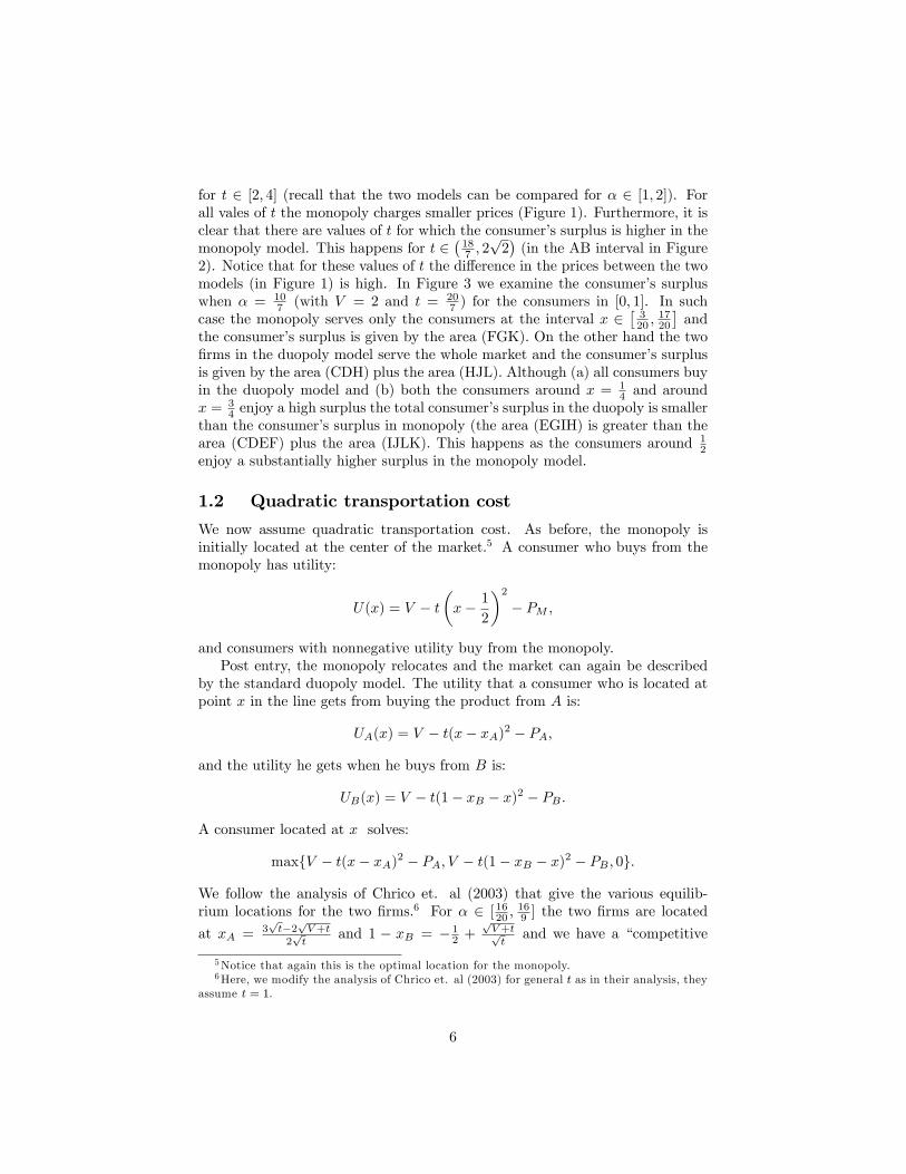
for t 2 [2; 4] (recall that the two models can be compared for � 2 [1; 2]). Forall vales of t the monopoly charges smaller prices (Figure 1). Furthermore, it isclear that there are values of t for which the consumer�s surplus is higher in themonopoly model. This happens for t 2

�187 ; 2

p2�(in the AB interval in Figure

2). Notice that for these values of t the di¤erence in the prices between the twomodels (in Figure 1) is high. In Figure 3 we examine the consumer�s surpluswhen � = 10

7 (with V = 2 and t = 207 ) for the consumers in [0; 1]. In such

case the monopoly serves only the consumers at the interval x 2�320 ;

1720

�and

the consumer�s surplus is given by the area (FGK). On the other hand the two�rms in the duopoly model serve the whole market and the consumer�s surplusis given by the area (CDH) plus the area (HJL). Although (a) all consumers buyin the duopoly model and (b) both the consumers around x = 1

4 and aroundx = 3

4 enjoy a high surplus the total consumer�s surplus in the duopoly is smallerthan the consumer�s surplus in monopoly (the area (EGIH) is greater than thearea (CDEF) plus the area (IJLK). This happens as the consumers around 1

2enjoy a substantially higher surplus in the monopoly model.

1.2 Quadratic transportation cost

We now assume quadratic transportation cost. As before, the monopoly isinitially located at the center of the market.5 A consumer who buys from themonopoly has utility:

U(x) = V � t�x� 1

2

�2� PM ;

and consumers with nonnegative utility buy from the monopoly.Post entry, the monopoly relocates and the market can again be described

by the standard duopoly model. The utility that a consumer who is located atpoint x in the line gets from buying the product from A is:

UA(x) = V � t(x� xA)2 � PA;

and the utility he gets when he buys from B is:

UB(x) = V � t(1� xB � x)2 � PB :

A consumer located at x solves:

maxfV � t(x� xA)2 � PA; V � t(1� xB � x)2 � PB ; 0g:

We follow the analysis of Chrico et. al (2003) that give the various equilib-rium locations for the two �rms.6 For � 2 [ 1620 ;

169 ] the two �rms are located

at xA = 3pt�2

pV+t

2pt

and 1 � xB = � 12 +

pV+tptand we have a �competitive

5Notice that again this is the optimal location for the monopoly.6Here, we modify the analysis of Chrico et. al (2003) for general t as in their analysis, they

assume t = 1.

6

equilibrium with full supply�type of equilibrium. In fact, here, the consumersat the endpoints of the product space enjoy a positive surplus and the consumerat x = 1

2 does not enjoy a positive surplus.7 For � 2 [ 169 ;

163 ] the two �rms

are located at the two quartiles and we have a touching equilibrium with fullsupply, in which the consumers at x = 0; x = 1 and x = 1

2 have zero utility.Finally, for � > 16

3 the two �rms form two (local) monopolies.We again consider values of � for which the optimal price of the monopoly

is an interior solution. This happens for � � 43 . We follow the analysis of the

previous section. We have the following Lemma:

Lemma 3 With quadratic transportation cost, the optimal price for the monopolythat is located at x = 1

2 is an interior solution for � �43 . In such case all con-

sumers in [ 12 �Vp3ptV; 12 +

Vp3ptV] buy. The monopoly�s price is 2V

3 its pro�ts

are 4V 2

3p3ptVthe consumer�s surplus is 4V

ptV

9p3t

and total welfare is 16V 2

9p3ptV.

When we have two �rms and for 1620 � � �

169 ; the price and the total pro�ts

are �2t+2ptpV + t, the consumer�s surplus is � 1

2

pt( 7

pt

6 �pV + t) and total

welfare is � 31t12 +

52

ptpV + t .

When we have two �rms, for 169 � � �

163 the price and the total pro�ts are

V � t16 the consumer�s surplus is

t24 and total welfare is V �

t48 .

The proof is in the Appendix. It is easy to prove the following Proposition:

Proposition 4 For quadratic transportation cost post entry: Prices increase for43 � � <

163 . Prices remain the same for � =

163 . Consumer�s surplus decrease

for 43 � � <

8 3p23 . Consumer�s surplus remains the same for � = 8 3p2

3 .

The proof can be easily derived if we compare the prices and the consumer�ssurplus in the monopoly model with those in the duopoly models for 1612 � � �

169

and 169 � � �

163 and can be found in the Appendix.

First notice that the monopoly sells only to a 12+

Vp3ptV�( 12�

Vp3ptV) = 2p

3�

mass of consumers around 12 . However, the monopoly price is smaller than the

price in the duopoly model for both types of equilibria.8 Although the consumerswho are located around xA and 1 � xB enjoy a positive surplus this is muchsmaller than the surplus that enjoy the consumers around the center beforeentry. For this reason, the consumer surplus is greater in the monopoly, for lowvalues of �.In Figures 4, 5 we compare the consumer�s surplus when V = 2. For this V

the acceptable values for t are: t 2�3212 ;

322

�in the duopoly model and t 2

�3220 ;1

�in the monopoly model. As the two models can be compared for � 2 [ 1612 ;

163 ]

we compare them for 3212 � t � 32

3 . For all vales of t the monopoly chargessmaller prices (Figure 4). The consumer�s surplus is higher in the monopolymodel when t < 16 3p2

3 (in the interval ab in Figure 5). Notice that for these

7The above hold also for � 2 [ 1633; 1620). However, in this range of �, the two �rms are

located outside of [0; 1], a possibility that we do not examine.8The price remains the same when � = 16

3.

7

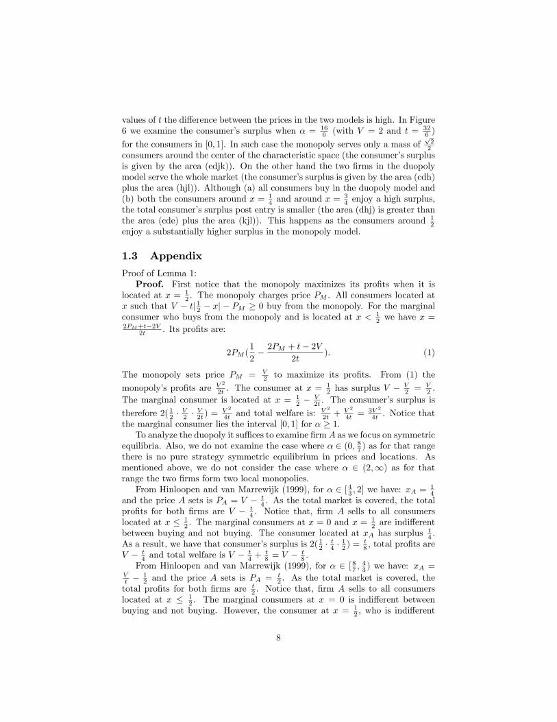
values of t the di¤erence between the prices in the two models is high. In Figure6 we examine the consumer�s surplus when � = 16

6 (with V = 2 and t = 326 )

for the consumers in [0; 1]. In such case the monopoly serves only a mass ofp22

consumers around the center of the characteristic space (the consumer�s surplusis given by the area (edjk)). On the other hand the two �rms in the duopolymodel serve the whole market (the consumer�s surplus is given by the area (cdh)plus the area (hjl)). Although (a) all consumers buy in the duopoly model and(b) both the consumers around x = 1

4 and around x =34 enjoy a high surplus,

the total consumer�s surplus post entry is smaller (the area (dhj) is greater thanthe area (cde) plus the area (kjl)). This happens as the consumers around 1

2enjoy a substantially higher surplus in the monopoly model.

1.3 Appendix

Proof of Lemma 1:Proof. First notice that the monopoly maximizes its pro�ts when it is

located at x = 12 . The monopoly charges price PM . All consumers located at

x such that V � tj 12 � xj � PM � 0 buy from the monopoly. For the marginalconsumer who buys from the monopoly and is located at x < 1

2 we have x =2PM+t�2V

2t . Its pro�ts are:

2PM (1

2� 2PM + t� 2V

2t). (1)

The monopoly sets price PM = V2 to maximize its pro�ts. From (1) the

monopoly�s pro�ts are V 2

2t . The consumer at x =12 has surplus V �

V2 =

V2 .

The marginal consumer is located at x = 12 �

V2t . The consumer�s surplus is

therefore 2( 12 �V2 �

V2t ) =

V 2

4t and total welfare is:V 2

2t +V 2

4t =3V 2

4t . Notice thatthe marginal consumer lies the interval [0; 1] for � � 1.To analyze the duopoly it su¢ ces to examine �rmA as we focus on symmetric

equilibria. Also, we do not examine the case where � 2 (0; 87 ) as for that rangethere is no pure strategy symmetric equilibrium in prices and locations. Asmentioned above, we do not consider the case where � 2 (2;1) as for thatrange the two �rms form two local monopolies.From Hinloopen and van Marrewijk (1999), for � 2 [ 43 ; 2] we have: xA =

14

and the price A sets is PA = V � t4 . As the total market is covered, the total

pro�ts for both �rms are V � t4 . Notice that, �rm A sells to all consumers

located at x � 12 . The marginal consumers at x = 0 and x =

12 are indi¤erent

between buying and not buying. The consumer located at xA has surplus t4 .

As a result, we have that consumer�s surplus is 2( 12 �t4 �

12 ) =

t8 , total pro�ts are

V � t4 and total welfare is V �

t4 +

t8 = V �

t8 .

From Hinloopen and van Marrewijk (1999), for � 2 [ 87 ;43 ) we have: xA =

Vt �

12 and the price A sets is PA = t

2 . As the total market is covered, thetotal pro�ts for both �rms are t

2 . Notice that, �rm A sells to all consumerslocated at x � 1

2 . The marginal consumers at x = 0 is indi¤erent betweenbuying and not buying. However, the consumer at x = 1

2 , who is indi¤erent

8

from buying from either �rm, has surplus 2V � 3t2 . The consumer located

at xA has surplus V � t2 . As a result, we have that consumer�s surplus is

2(( 12 � (V �t2 ) � (

Vt �

12 )) +

12 (2V �

3t2 + V �

t2 ) � (

12 �

Vt +

12 )) = 4V �

2V 2

t � 7t4

and total welfare is 4V � 2V 2

t � 5t4 .

Proof of Proposition 2Proof. For � 2 [ 87 ;

43 ) the price in the duopoly model is

t2 and the price in

the monopoly model is V2 . As � =

tV > 1, post entry the price increases.

For � 2 [ 87 ;43 ) the di¤erence in consumer�s surplus between the monopoly

and the duopoly models is:

V 2

4t��4V � 2V

2

t� 7t4

�= �4V + 9V

2

4t+7t

4:

The di¤erence is zero for t = V and t = 9V7 . Notice that the di¤erence is

positive for t > 9V7 as its derivative with respect to t, which is equal to 7

4 �9V 2

4t2

is positive for t > 3Vp7and 3Vp

7< 9V

7 .

For � 2 [ 43 ; 2] the price in the duopoly model is V �t4 . We have:

V � t

4>V

2=) V

2>t

4=) � < 2;

post entry the price increases, and only for � = 2 prices remain the same.For � 2 [ 43 ; 2] the di¤erence in consumer�s surplus between the monopoly

and the duopoly models is:V 2

4t� t

8;

which is positive for � <p2, and zero for � =

p2.

Proof of Lemma 3:Proof. We now examine the monopoly at x = 1

2 model. The consumer atx who buys from the monopolist who is located at x = 1

2 and charges price

PM has utility V � t�12 � x

�2 � PM . The price PM is such that the marginalconsumer who is located at x� has zero surplus. We therefore have: PM =

V �t�12 � x

��2 =) x� = 12��V�PM

t

� 12 and x� = 1

2+�V�PM

t

� 12 . The monopolist

who is located at x = 12 maximizes its pro�ts:

2PM

1

2� 1

2��V � PM

t

� 12

!!:

From the �rst order condition we have PM = 2V3 . We have x

� = 12 �

Vp3tV;

x� = 12+

Vp3tV. As we require 0 � x� � 1 we also require V � 3t

4 =) � � 43 . The

pro�ts are 4V 2

3p3ptV. The consumer located at x who buys from the monopoly

has surplus: V � t( 12 � x)2 � 2V

3 . The consumer�s surplus is:Z 12+

Vp3tV

12�

Vp3tV

�V � t(1

2� x)2 � 2V

3

�dx =

4VptV

9p3t

;

9

and total welfare is 16V 2

9p3ptV.

Following Chrico et. al (2003), when we have two �rms, for 1620 � � � 16

9

the location of �rm A is, xA =3pt�2

pV+t

2pt

and the location of B is: 1 � xB =� 12 +

pV+tpt. The price and the total pro�ts are �2t+ 2

ptpV + t. The surplus

of a consumer located at x who buys from A is:

V � t�x�

�3pt� 2

pV + t

2pt

��2� (�2t+ 2

ptpV + t) =

�14

pt(�1 + 2x)(4

pV + t+

pt(�5 + 2x)):

The consumer�s surplus is:

2

Z 12

0

��14

pt(�1 + 2x)(4

pV + t+

pt(�5 + 2x))

�dx =

�12

pt

�7pt

6�pV + t

�and total welfare is � 31t

12 +52

ptpV + t .

For 169 � � <

163 the price and the total pro�ts are V � t

16 . The consumerlocated at x and buys form A has surplus

V � t�1

4� x�2��V � t

16

�=1

2t(1� 2x)x;

and the total consumer�s surplus is

2

Z 12

0

1

2t(1� 2x)xdx = t

24;

and total welfare is V � t16 +

t24 = V �

t48 .

Proof of Proposition 4.Proof. For 1612 � � �

169 we �rst compare the prices in the two models. We

have:

�2t+ 2ptpV + t >

2V

3=) 2

ptpV + t >

2V

3+ 2t;

and we have:

t(V + t) >

�V

3+ t

�2=) tV

3>V 2

9=) t

V>1

3;

which holds as 1612 � �.

We now compare consumer�s surplus for the monopoly at x = 12 and the

duopoly at xA =3pt�2

pV+t

2pt

models. The di¤erence in the consumer�s surplusis:

4VptV

9p3t

���12

pt

�7pt

6�pV + t

��: (2)

10

Its derivative with respect to V is: 2V3p3ptV�

pt

4pt+V

and is positive in this

interval as it is positive for the minimum value of V in the interval,9 that is for

V = 9t16 . We have

2V3p3ptV�

pt

4pt+V

���V= 9t16= � 1

5 +1

2p3> 0. It therefore su¢ ces

to show that the di¤erence is positive for V = 9t16 . This holds as for V =

9t16 , (2)

is equal to 148 (�2t+ 3

p3t) > 0.

For 169 � � �

163 we �rst compare the prices in the two models. We have:

V � t

16>2V

3=) V

3>t

16;

which holds as inequality for � < 163 and as equality when � =

163 .

We now compare consumer�s surplus for the monopoly at x = 12 and the

duopoly at the quartiles models. The di¤erence in the consumer�s surplus is:

4VptV

9p3t

� t

24:

First notice that 169 � � �163 ()

3t16 � V �

9t16 . The derivative of

4VptV

9p3t

with

respect to V is: 2V3p3ptVand is positive. We have:

4VptV

9p3t

� t

24= 0 =) V =

3t

8 3p2:

As 3t16 <

3t8 3p2 <

9t16 the di¤erence is negative for V 2

h3t16 ;

3t8 3p2

�zero at 3t

8 3p2 and

positive for�

3t8 3p2 ;

9t16

i. In terms of �, the di¤erence is positive for � 2

h169 ;

8 3p23

�nd zero at � = 8 3p2

3 .

References

[1] Caves, R., M.D. Whinston, and M.A. Hurwitz (1991), Patent Expiration,Entry, and Competition in the U.S. Pharmaceutical Industry, BrookingsPapers in Economic Activity : Microeconomics, 1-48.

[2] Chen, Y., and M.H. Riordan (2007), Price and Variety in the Spokes Model,Economic Journal, 117, 897-921.

[3] Chen, Y., and M. H. Riordan (2008), Price increasing competition, RANDJournal of Economics, 39, 1042-1058.

[4] Chrico, A., Lambertini, L., and F. Zagonari (2003), How demand a¤ectsoptimal prices and product di¤erentiation, Papers in Regional Science, 82,555-568.

9We have: 1612� � � 16

9() 9t

16� V � 12t

16.

11

[5] Cowan, S., and Yin, X. (2008), Competition can harm consumers, Aus-tralian Economic Papers, 47, 3, 264-271.

[6] Goolsbee, A., and C., Syverson (2006), How do incumbents respond tothe threat of entry: Evidence from major airlines, University of Chicago,working paper.

[7] Grabowski, H. G., and J. M. Vernon (1992), Brand loyalty, entry and pricecompetition in pharmaceuticals after the 1984 Drug Act, Journal of Lawand Economics, 35: 331-350.

[8] Hinloopen, J., and C., van Marrewijk (1999), On the limits of the principleof minimum di¤erentiation, International Journal of Industrial Organiza-tion, 17, 735-750.

[9] Hotelling, H. (1929), Stability in competition, Economic Journal, 41-57.

[10] Lerner, A.P., and H.W. Singer (1937), Some notes on duopoly and spatialcompetition, Journal of Political Economy, 45, 145-186.

[11] Perlo¤, J.M., V.Y., Suslow and P.J., Seguin (2005), Higher prices fromentry: Pricing of brand-name drugs, mimeo.

[12] Rosenthal, R.W. (1980), A model in which an increase in the number ofsellers leads to a higher price, Econometrica, 48, 1575-1580.

[13] Schulz, N., and K. Stahl (1996), Do Consumers Search for the Higher Price?Oligopoly Equilibrium and Monopoly Optimum in Di¤erentiated-ProductsMarkets. Rand Journal of Economics, 27, 542-562.

[14] Sweeting, A. (2007), Dynamic product repositioning in di¤erentiated prod-uct markets: The case of format switching in the commercial radio industry,NBER working paper 13522.

[15] Stiglitz, J.E. (1987), Competition and the Number of Firms in a Market:Are Duopolists More Competitive Than Atomistic Markets?, Journal ofPolitical Economy, 95: 1041-1061.

[16] Thomadsen, R. (2007), Product positioning and competition: The role oflocation in the fast food industry, Marketing Science, 26, 792-804.

[17] Ward, M,R., J.P. Shimshack, J.M. Perlo¤, and Harris, J.M. (2002), Ef-fects of the private-label invasion in food industries, American Journal ofAgricultural Economics, 84, 961-973.

[18] Zhou, W. (2006), A simple model of entry that increases price levels andprice dispersion, Advances in Economic Analysis and Policy, 6, 1, Article7.

12

2.002.052.102.152.202.25

0.050.100.150.200.250.300.350.400.450.500.550.600.650.700.75 C0.80

Consumer's surplus (Linear cost)

0

0.1

0.2

0.3

0.4

0.5

0.6

2.1 2.25 2.4 2.55 2.7 2.85 3 3.15 3.3 3.45 3.6 3.75 3.9t

Figure 2

CS

MonopolyDuopoly

AB

Consumer's surplus (Linear cost)

0

0.2

0.4

0.6

0.8

1

1.2

0 0.08 0.15 0.23 0.3 0.38 0.45 0.53 0.6 0.68 0.75 0.83 0.9 0.98x

Figure 3

CS

Monopoly

Duopoly

C

D

E

F

G

H

I

J

K L

Prices (Linear cost)

0

0.2

0.4

0.6

0.8

1

1.2

1.4

2 2.1 2.2 2.3 2.4 2.5 2.6 2.7 2.8 2.9 3 3.1 3.2 3.3 3.4 3.5 3.6 3.7 3.8 3.9 4t

Figure 1

Pric

e

MonopolyDuopoly

Prices (Quadratic cost)

00.20.40.60.8

11.21.41.61.8

2

1.82 2.48 3.14 3.8 4.46 5.12 5.78 6.44 7.1 7.76 8.42 9.08 9.74 10.4t

Figure 4

Pric

e

MonopolyDuopoly

Consumer's surplus (Quadratic cost)

0

0.05

0.1

0.15

0.2

0.25

0.3

0.35

0.4

0.45

0.5

1.82 2.48 3.14 3.8 4.46 5.12 5.78 6.44 7.1 7.76 8.42 9.08 9.74 10.4t

Figure 5

CS

MonopolyDuopoly

b

a

Consumer's Surplus (Quadratic cost)

0

0.1

0.2

0.3

0.4

0.5

0.6

0.7

0 0.08 0.15 0.23 0.3 0.38 0.45 0.53 0.6 0.68 0.75 0.83 0.9 0.98x

Figure 6

CS

MonopolyDuopoly

c

d

eh

j

k l