Finite Sample Inference Methodsfor Simultaneous Equations and

Models with Unobserved and Generated Regressors1

Jean-Marie Dufour2 and Joanna Jasiak3

Universite de Montreal and York University

January 2000

1This work was supported by the Social Sciences and Humanities Research Council of Canada, the Nat-ural Sciences and Engineering Research Council of Canada and the Fonds FCAR (Government of Qu´ebec).The authors thank Lise Salvas and Claude Montmarquette for providing the data as well as Gordon Fisher,Denis Foug`ere, Christian Gouri´eroux, Helmut Lutkepohl, Edmond Malinvaud, Alain Monfort, Garry Phillips,Jim Stock, Mohamed Taamouti, Herman van Dijk, Eric Zivot, the Editor Frank Diebold and three anonymousreferees for helpful comments. This paper is a revised version of Dufour and Jasiak (1993).

2C.R.D.E, Universit´e de Montreal, C.P. 6128, Succursale Centre Ville, Montr´eal, Quebec H3C 3J7,Canada. TEL: 1 514 343 6557; FAX: 1 514 343 5831; e-mail:dufour@crde:umontreal:ca.

3Department of Economics, York University, 4700 Keele Street, Toronto, Ontario M3J 1P3, Canada. TEL:1 416 736 2100 extension 77045; FAX: 1 416 736 5987; e-mail:jasiakj@yorku:ca.

ABSTRACT

We propose finite sample tests and confidence sets for models with unobserved and generatedregressors as well as various models estimated by instrumental variables method. We study twodistinct approaches for various models considered by Pagan (1984). The first one is an instrumentsubstitution method which generalizes an approach proposed by Anderson and Rubin (1949) andFuller (1987) for different (although related) problems, while the second one is based on splittingthe sample. The instrument substitution method uses the instruments directly, instead of generatedregressors, in order to test hypotheses about the “structural parameters” of interest and build confi-dence sets. The second approach relies on “generated regressors”, which allows a gain in degreesof freedom, and a sample split technique. A distributional theory is obtained under the assumptionsof Gaussian errors and strictly exogenous regressors. We show that the various tests and confidencesets proposed are (locally) “asymptotically valid” under much weaker assumptions. The proper-ties of the tests proposed are examined in simulation experiments. In general, they outperform theusual asymptotic inference methods in terms of both reliability and power. Finally, the techniquessuggested are applied to a model of Tobin’sq and to a model of academic performance.

Key words: generated regressor; simultaneous equations; structural model; pivotal function;sample-split; Anderson-Rubin method; finite-sample inference; exact test; confidence region; in-strumental variables; Tobin’sq; academic performance.

RESUME

Nous proposons des tests et r´egions de confiance exactes pour des mod`eles comportant desvariables inobserv´ees ou des r´egresseurs estim´es de mˆeme que pour divers mod`eles estim´es parla methode des variables instrumentales. De fac¸on plus sp´ecifique, nous ´etudions deux approchesdiff erentes pour divers mod`eles consid´eres par Pagan (1984). La premi`ere est une m´ethode desubstitution d’instruments qui g´eneralise des techniques propos´ees par Anderson et Rubin (1949)et Fuller (1984) pour des probl`emes differents, tandis que la seconde m´ethode est fond´ee sur unesubdivision de l’echantillon. La m´ethode de substitution d’instruments utilise directement les in-struments disponibles, plutˆot que des r´egresseurs estim´es, afin de tester des hypoth`eses et construiredes regions de confiance sur les “param`etres structuraux” du mod`ele. La seconde m´ethode s’appuiesur des r´egresseurs estim´es, ce qui permet un gain de degr´es de libert´e, ainsi que sur une techniquede subdivision de l’´echantillon. Nous fournissons une th´eorie distributionnelle exacte sous une hy-pothese de normalit´e des perturbations et de r´egresseurs strictement exog`enes. Nous montrons queles tests et r´egions de confiance ainsi obtenus sont aussi (localement) “asymptotiquement valides”sous des hypoth`eses distributionnelles beaucoup plus faibles. Nous ´etudions les propri´etes des testsproposes dans le cadre d’une exp´erience de simulation. En g´eneral, celles-ci sont plus fiables et ontune meilleure puissance que les techniques traditionnelles. Finalement, les techniques propos´eessont appliqu´eesa un modele duq de Tobin eta un modele de performance scolaire.

Mots-clefs: regresseur estim´e; equations simultan´ees; mod`ele structurel; fonction pivotale; subdivi-sion d’echantillon; methode d’Anderson-Rubin; variables instrumentales; inf´erence `a distance finie;test exact; r´egion de confiance; variables instrumentales;q de Tobin; performance scolaire.

Contents

1 Introduction 1

2 Exact inference by instrument substitution 3

3 Inference with generated regressors 6

4 Joint tests on Æ and 7

5 Inference with a surprise variable 9

6 Inference on general parameter transformations 10

7 Asymptotic validity 12

8 Monte Carlo study 13

9 Empirical illustrations 19

10 Conclusions 22

1 Introduction

A frequent problem in econometrics and statistics consists in making inferences on models whichcontain unobserved explanatory variables, such as expectational or latent variables and variablesobserved with error; see, for example, Barro (1977), Pagan (1984, 1986) and the survey of Oxleyand McAleer (1993). A common solution to such problems is based on using instrumental variablesto replace the unobserved variables by proxies obtained from auxiliary regressions (generated re-gressors). It is also well known that using such regressors raises difficulties for making tests andconfidence sets, and it is usually proposed to replace ordinary least squares (OLS) standard errorsby instrumental variables (IV) based standard errors; see Pagan (1984, 1986) and Murphy and Topel(1985). In any case, all the methods proposed to deal with such problems only have an asymptoticjustification, which means that the resulting tests and confidence sets can be extremely unreliablein finite samples. In particular, such difficulties occur in situations involving “weak instruments”,a problem which has received considerable attention recently; see, for example, Nelson and Startz(1990a, b), Buse (1992), Maddala and Jeong (1992), Bound, Jaeger and Baker (1993, 1995), An-grist and Krueger (1994), Hall, Rudebusch and Wilcox (1996), Dufour (1997), Staiger and Stock(1997) and Wang and Zivot (1997) [for some early results relevant to the same issue, see also Nagar(1959), Richardson (1968) and Sawa (1969)].

In this paper, we treat these issues from a finite sample perspective and we propose finite sampletests and confidence sets for models with unobserved and generated regressors. We also consider anumber of related problems in the more general context of linear simultaneous equations. To get re-liable tests and confidence sets, we emphasize the derivation of truly pivotal (or boundedly pivotal)statistics, as opposed to statistics which are only asymptotically pivotal; for a general discussionof the importance of such statistics for inference, see Dufour (1997). We study two distinct ap-proaches for various models considered by Pagan (1984). The first one is an instrument substitutionmethod which generalizes an approach proposed by Anderson and Rubin (1949) and Fuller (1987)for different (although related) problems, while the second one is based on splitting the sample.The instrument substitution method uses the instruments directly, instead of generated regressors,in order to test hypotheses and build confidence sets about “structural parameters”. The secondapproach relies on “generated regressors”, allowing a gain in degrees of freedom, and a samplesplit technique. Depending on the problem considered, we derive either exactsimilar tests (andconfidence sets) or conservative procedures. The hypotheses for which we obtain similar tests (andcorrespondingly similar confidence sets) include: a) hypotheses which set the value of the unob-served (expected) variable coefficient vector [as in Anderson and Rubin (1949) and Fuller (1987)];b) analogous restrictions taken jointly with general linear constraints on the coefficients of the (ob-served) exogenous variables in the equation of interest; and c) hypothesis about the coefficients of“surprise” variables when such variables are included in the equation. Tests for these hypotheses arebased on Fisher-type statistics, but the confidence sets typically involve nonlinear (although quitetractable) inequalities. In particular, when only one unobserved variable (or endogenous explana-tory variable) appears in the model, the confidence interval for the associated coefficient can becomputed easily on finding the roots of a quadratic polynomial. Note that Anderson-Rubin-typemethods have not previously been suggested in the context of the general Pagan (1984) setup; fur-ther, problems such as those described in b) and c) above have not apparently been considered at allfrom this perspective.

In the case of the instrument substitution method, the tests and confidence sets so obtained can beinterpreted as likelihood ratio (LR) procedures (based on appropriately chosen reduced form alter-natives), or equivalently as profile likelihood techniques [for further discussion of such techniques,see Bates and Watts (1988, Chapter 6), Meeker and Escobar (1995) and Chen and Jennrich (1996)].

1

The exact distributional theory is obtained under the assumptions of Gaussian errors and strictlyexogenous regressors, which ensures that we have well-defined testable models. Although we stresshere applications to models with unobserved regressors, the extensions of Anderson–Rubin (AR)procedures that we discuss are also of interest for inference in various structural models which areestimated by instrumental variable methods (e.g., simultaneous equations models). Furthermore, weobserve that the tests and confidence sets proposed are (locally) “asymptotically valid” under muchweaker distributional assumptions (which may involve non-Gaussian errors and weakly exogenousinstruments).

It is important to note that the confidence sets obtained by the methods described above, unlikeWald-type confidence sets, are unbounded with non-zero probability. As emphasized from a generalperspective in Dufour (1997), this is a necessary property of any valid confidence set for a parameterthat may not be identifiable on some subset of the parameter space. As a result, confidence proce-dures that do not have this property have true level zero, and the sizes of the corresponding tests(like Wald-type tests) must deviate arbitrarily from their nominal levels. It is easy to see that suchdifficulties occur in models with unobserved regressors, models with generated regressors, simulta-neous equations models, and different types of the error-in-variables models. In the context of thefirst type of model, we present below simulation evidence that strikingly illustrates these difficul-ties. In particular, our simulation results indicate that tests based on instrument substitution methodshave good power properties with respect to Wald-type tests, a feature previously pointed out for theAR tests by Maddala (1974) in a comparative study for simultaneous equations [on the power ofAR tests, see also Revankar and Mallela (1972)]. Furthermore, we find that generated regressorssample-split tests perform better when the generated regressors are obtained from a relatively smallfraction of the sample (e.g., 10% of the sample) while the rest of the sample is used for the mainregression (in which generated regressors are used).

An apparent shortcoming of the similar procedures proposed above, and probably one of thereasons why AR tests have not become widely used, is the fact that they are restricted to testinghypotheses which specify the values of the coefficients of all the endogenous (or unobserved) ex-planatory variables, excluding the possibility of considering a subset of coefficients (e.g., individualcoefficients). We show that inference on individual parameters or subvectors of coefficients is how-ever feasible by applying a projection technique analogous to the ones used in Dufour (1989, 1990),Dufour and Kiviet (1996, 1998) and Kiviet and Dufour (1997). We also show that such techniquesmay be used for inference on general possibly nonlinear transformations of the parameter vector ofinterest.

The plan of the paper is as follows. In Section 2, we describe the main model which may con-tain several unobserved variables (analogous to the “anticipated” parts of those variables), and weintroduce the instrument substitution method for this basic model with various tests and confidencesets for the coefficients of the unobserved variables. In Section 3, we propose the sample splitmethod for the same model with again the corresponding tests and confidence sets. In Section 4,we study the problem of testing joint hypotheses about the coefficients of the unobserved variablesand various linear restrictions on the coefficients of other (observed) regressors in the model. Sec-tion 5 extends these results to a model which also contains error terms of the unobserved variables(the “unanticipated” parts of these variables). In Section 6, we consider the problem of makinginference about general nonlinear transformations of model coefficients. Then, in Section 7, wediscuss the “asymptotic validity” of the proposed procedures proposed under weaker distributionalassumptions. Section 8 presents the results of simulation experiments in which the performance ofour methods is compared with some widely used asymptotic procedures. Section 9 presents appli-cations of the proposed methods to a model of Tobin’sq and to an economic model of educationalperformance. The latter explains the relationship between students’ academic performance, their

2

personal characteristics and some socio-economic factors. The first example illustrates inferencein presence of good instruments, while in the second example only poor instruments are available.As expected, confidence intervals for Tobin’sq based on the Wald-type procedures largely coin-cide with those resulting from our methods. On the contrary, large discrepancies arise betweenthe confidence intervals obtained from the asymptotic and the exact inference methods when poorinstruments are used. We conclude in Section 10.

2 Exact inference by instrument substitution

In this section, we develop finite sample inference methods based on instrument substitution meth-ods for models with unobserved and generated regressors. We first derive general formulae for thetest statistics and then discuss the corresponding confidence sets. We consider the following basicsetup which includes as special cases Models 1 and 2 studied by Pagan (1984):

y = Z�Æ +X + e ;(2.1)

Z� =WB + U� ; Z = Z� + V�(2.2)

wherey is aT�1 vector of observations on a dependent variable,Z� is aT�Gmatrix of unobservedvariables,X is aT � K matrix of exogenous explanatory variables in the structural model,Z isa T � G matrix of observed variables,W is a T � q matrix of variables related toZ�; whilee = (e1; : : : ; eT )

0; U� = [u0�1; : : : ; u

0�T ]

0 andV� = [v0�1; : : : ; v0�T ]

0 areT � 1 andT � G matricesof disturbances. The matrices of unknown coefficientsÆ; ; andB have dimensions respectivelyG � 1; K � 1 andq � G: In order to handle common variables in both equations (2.1) and (2.2),like for example the constant term, we allow for the presence of common columns in the matricesW andX. In the setup of Pagan (1984),U� is assumed to be identically zero(U� = 0); et andv�tare uncorrelated[E(etv�t) = 0]; and the exogenous regressorsX are excluded from the “structural”equation (2.1). In some cases below, we will need to reinstate some of the latter assumptions.

The finite sample approach we adopt in this paper requires additional assumptions, especially onthe distributional properties of the error term. Since (2.2) entailsZ =WB+V whereV = U�+V�;

we will suppose the following conditions are satisfied:

X andW are independent ofe andV� ;(2.3)

rank (X) = K ; 1 � rank (W ) = q < T ; G � 1 ; 1 � K +G < T ;(2.4)

(et; v0

�t)0 ind� N [0; ] ; t = 1; : : : ; T ;(2.5)

det() > 0 :(2.6)

If K = 0, X is simply dropped from equation (2.1). Note that no assumption on the distribution ofU� is required. Assumptions (2.3) – (2.6) can be relaxed if they are replaced by assumptions on theasymptotic behavior of the variables asT !1. Results on the asymptotic “validity” of the variousprocedures proposed in this paper are presented in Section 7.

Let us now consider the null hypothesis:

H0 : Æ = Æ0 :(2.7)

The instrument substitution method is based on replacing the unobserved variable by a set of instru-ments. First, we substitute (2.2) into (2.1):

y = (Z � V�)Æ +X + e = ZÆ +X + (e� V�Æ) :(2.8)

3

Then subtractingZÆ0 on both sides of (2.8), we get:

y � ZÆ0 =WB(Æ � Æ0) +X + u(2.9)

whereu = e � V�Æ0 + U�(Æ � Æ0): Now suppose thatW andX haveK2 columns in common(0 � K2 < q) while the other columns ofX are linearly independent ofW :

W = [W1; X2] ; X = [X1; X2] ; rank [W1; X1; X2] = q1 +K < T(2.10)

whereW1, X1 andX2 areT � q1, T � K1 andT � K2 matrices, respectively (K = K1 + K2,q = q1 +K2). We can then rewrite (2.9) as

y � ZÆ0 =W1Æ1� +X � + u(2.11)

whereÆ1� = B1(Æ � Æ0), 2� = 2 +B2(Æ � Æ0); � = ( 01; 02�)

0; Bi is aKi �G matrix (i = 1;

2) andB = [B01; B

02]0:

It is easy to see that model (2.11) underH0 satisfies all the assumptions of the classical linearmodel. Furthermore, sinceÆ1� = 0 whenÆ = Æ0, we can testH0 by a standardF -test of the nullhypothesis

H0� : Æ1� = 0 :(2.12)

ThisF -statistic has the form

F (Æ0; W1) =(y � ZÆ0)

0P (M(X)W1) (y � ZÆ0)=q1

(y � ZÆ0)0M([W1; X]) (y � ZÆ0)=(T � q1 �K)(2.13)

whereP (A) = A(A0A)�1

A0 andM(A) = IT � P (A) for any full column rank matrixA: When

Æ = Æ0, we haveF (Æ0; W1) � F (q1; T � q1�K); so thatF (Æ0; W1) > F (�; q1; T � q1�K) isa critical region with level� for testingÆ = Æ0; whereP [F (Æ0; W1) � F (�; q1; T � q1 �K)] =

1 � � : The essential ingredient of the test is the fact thatq1 � 1, i.e. some instruments must beexcluded fromX in (2.1). On the other hand, the usual order condition for “identification”(q1 � G)

is not necessary for applying this procedure. In other words, it is possible to test certain hypothesesaboutÆ even if the latter vector is not completely identifiable. It is then straightforward to see thatthe set

CÆ(�) = fÆ0 : F (Æ0; W1) � F (�; q1; T � q1 �K)g(2.14)

is a confidence set with level1� � for the coefficientÆ. The tests based on the statisticF (Æ0; W1)

and the above confidence set generalizes the procedure proposed by Fuller (1987, pp. 16–17) for amodel with one unobserved variable(G = 1) andX limited to a constant variable(K = 1):

Consider now the case whereZ is aT � 1 vector andX is aT �K matrix. In this case, theconfidence set (2.14) for testingH0 : Æ = Æ0 has the following general form:

CÆ(�) =

�Æ0 :

(y � ZÆ0)0A1(y � ZÆ0)

(y � ZÆ0)0A2(y � ZÆ0)��2

q1� F�

�(2.15)

where F� = F (�; q1; T � q1 � K) and �2 = T � q1 � K and the matricesA1 =

P (M(X)W1); A2 = M([W1; X]): Since(�2=q1) only takes positive values, the inequality in(2.15) is equivalent to the quadratic inequality:

aÆ20 + bÆ0 + c � 0(2.16)

wherea = Z0CZ; b = �2y0CZ; c = y

0Cy; C = A1 �G�A2 andG� = (q1=�2)F�:

4

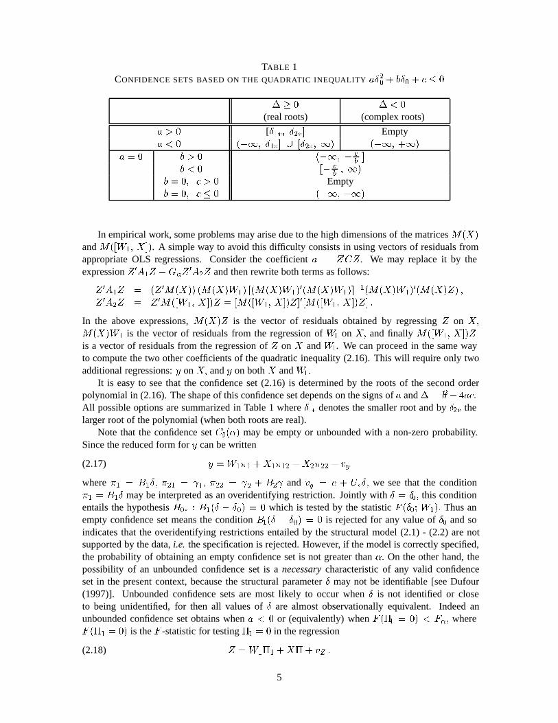
TABLE 1CONFIDENCE SETS BASED ON THE QUADRATIC INEQUALITYaÆ20 + bÆ0 + c � 0

� � 0 � < 0

(real roots) (complex roots)

a > 0 [Æ1�; Æ2�] Emptya < 0 (�1; Æ1�] [ [Æ2�; 1) (�1; +1)

a = 0 b > 0��1; �

cb

�b < 0

��

cb; 1

�b = 0; c > 0 Emptyb = 0; c � 0 (�1; +1)

In empirical work, some problems may arise due to the high dimensions of the matricesM(X)

andM([W1; X]). A simple way to avoid this difficulty consists in using vectors of residuals fromappropriate OLS regressions. Consider the coefficienta = Z

0CZ. We may replace it by the

expressionZ0A1Z �G�Z

0A2Z and then rewrite both terms as follows:

Z0A1Z = (Z 0

M(X)) (M(X)W1) [(M(X)W1)0(M(X)W1)]

�1(M(X)W1)0(M(X)Z) ;

Z0A2Z = Z

0M([W1; X])Z = [M([W1; X])Z]0[M([W1; X])Z] :

In the above expressions,M(X)Z is the vector of residuals obtained by regressingZ on X;

M(X)W1 is the vector of residuals from the regression ofW1 on X; and finallyM([W1; X])Z

is a vector of residuals from the regression ofZ onX andW1. We can proceed in the same wayto compute the two other coefficients of the quadratic inequality (2.16). This will require only twoadditional regressions:y onX; andy on bothX andW1:

It is easy to see that the confidence set (2.16) is determined by the roots of the second orderpolynomial in (2.16). The shape of this confidence set depends on the signs ofa and� = b

2� 4ac:

All possible options are summarized in Table 1 whereÆ1� denotes the smaller root and byÆ2� thelarger root of the polynomial (when both roots are real).

Note that the confidence setCÆ(�) may be empty or unbounded with a non-zero probability.Since the reduced form fory can be written

y =W1�1 +X1�12 +X2�22 + vy(2.17)

where�1 = B1Æ; �21 = 1; �22 = 2 + B2 and vy = e + U�Æ; we see that the condition�1 = B1Æ may be interpreted as an overidentifying restriction. Jointly withÆ = Æ0; this conditionentails the hypothesisH0� : B1(Æ � Æ0) = 0 which is tested by the statisticF (Æ0; W1): Thus anempty confidence set means the conditionB1(Æ � Æ0) = 0 is rejected for any value ofÆ0 and soindicates that the overidentifying restrictions entailed by the structural model (2.1) - (2.2) are notsupported by the data,i.e. the specification is rejected. However, if the model is correctly specified,the probability of obtaining an empty confidence set is not greater than�: On the other hand, thepossibility of an unbounded confidence set is anecessary characteristic of any valid confidenceset in the present context, because the structural parameterÆ may not be identifiable [see Dufour(1997)]. Unbounded confidence sets are most likely to occur whenÆ is not identified or closeto being unidentified, for then all values ofÆ are almost observationally equivalent. Indeed anunbounded confidence set obtains whena < 0 or (equivalently) whenF (�1 = 0) < F�; whereF (�1 = 0) is theF -statistic for testing�1 = 0 in the regression

Z =W1�1 +X� + vZ :(2.18)

5

In other words, the confidence interval (2.15) is unbounded if and only if the coefficients of theexogenous regressors inW1 [which is excluded from the structural equation (2.1)] are not signifi-cantly related toZ at level� : i.e:, W1 can be interpreted as a matrix of “weak instruments” forZ:

In contrast, Wald-type confidence sets forÆ are typically bounded with probability one, so their truelevel must be zero. Note finally that an unbounded confidence set can be informative:e.g., the set(�1; Æ1�] [ [Æ2�; 1) may exclude economically important values ofÆ (Æ = 0 for example).

3 Inference with generated regressors

Test statistics similar to those of the previous section may alternatively be obtained from linear re-gressions with generated regressors. To obtain finite sample inferences in such contexts, we proposeto compute adjusted values from an independent sample. In particular, this can be done by applyinga sample split technique.

Consider again the model described by (2.1) to (2.6). In (2.9), a natural thing to do wouldconsist in replacingWB by WB, whereB is an estimator ofB. TakeB = (W 0

W )�1W

0Z; the

least squares estimate ofB based on (2.2). Then we have:

y � ZÆ0 =WB(Æ � Æ0) +X + [u+W (B � B) (Æ � Æ0)] = ZÆ0� +X + u�(3.1)

whereÆ0� = Æ � Æ0 andu� = e � V�Æ0 + [U� +W (B � B) ](Æ � Æ0). Again, the null hypothesisÆ = Æ0 may be tested by testingH0� : Æ0� = 0 in model (3.1). Here the standardF statistic forH0�

is obtained by replacingW1 by Z in (2.13),i.e.

F (Æ0; Z) =(y � ZÆ0)

0P (M(X)Z) (y � ZÆ0)=G

(y � ZÆ0)0M([Z; X]) (y � ZÆ0)=(T �G�K);(3.2)

if K = 0 [noX matrix in (2.1)], we conventionally setM(X) = IT and[Z; X] = Z: However, toget a null distribution forF (Æ0; Z), we will need further assumptions. For example, in addition tothe assumptions (2.1) to (2.6), suppose, as in the original Pagan (1984) setup, that

e andV � U� + V� are independent.(3.3)

In this case, whenÆ = Æ0 = 0; Z andu� are independent and, conditional onZ, model (3.1) satisfiesall the assumptions of the classical linear model (with probability 1). Thus the null distribution ofthe statisticF (0; Z) for testingÆ0 = 0 is F (G; T �G�K). Unfortunately, this property does notextend to the more general statisticF (Æ0; Z) whereÆ0 6= 0 becauseZ andu� are not independentin this case. A similar observation (in an asymptotic context) was made by Pagan (1984).

To deal with more general hypotheses, suppose now that an estimate~B of B such that

~B is independent ofe andV�(3.4)

is available, and replaceZ =WB by ~Z =W ~B in (3.1). We then get

y � ZÆ0 = ~ZÆ0� +X + u��(3.5)

whereu�� = e � V�Æ0 + [U� +W (B � ~B)] (Æ � Æ0). Under the assumptions (2.1) – (2.6) withÆ = Æ0 and conditional on~Z (or ~B), model (3.5) satisfies all the assumptions of the classical linearmodel and the usualF -statistic for testingÆ0� = 0;

F (Æ0; ~Z) =(y � ZÆ0)

0P (M(X) ~Z)(y � ZÆ0)=G

(y � ZÆ0)0M([ ~Z; X])(y � ZÆ0)=(T �G�K)(3.6)

6

where the usual notation has been adopted, follows anF (G; T�G�K) distribution. Consequently,the critical regionF (Æ0; ~Z) > F (�; G; T � G �K) has size�: Note that condition (3.3) is notneeded for this result to hold. Furthermore

~CÆ(�) = fÆ0 : F (Æ0; ~Z) � F (�; G; T �G�K)g(3.7)

is a confidence set forÆ with size1 � �: For scalarÆ (G = 1), this confidence set takes a formsimilar to the one in (2.15), except thatA1 = P (M(X) ~Z) andA2 =M([ ~Z; X]):

A practical problem here consists in finding the independent estimate~B. Under the assumptions(2.1) – (2.6), this can be done easily by splitting the sample. LetT = T1 + T2, whereT1 >

G +K andT2 � q, and write:y = (y0(1) ; y0

(2))0; X = (X 0

(1) ; X0

(2))0; Z = (Z 0

(1) ; Z0

(2))0; W =

(W 0

(1) ; W0

(2))0; e = (e0(1) ; e

0

(2))0; V� = (V 0

�(1) ; V0

�(2))0 and(U 0

�(1) ; U0

�(2))0; where the matricesy(i);

X(i) ; Z(i) ; W(i) ; e(i) ; V�(i) andU�(i) haveTi rows(i = 1; 2): Consider now the equation

y(1) � Z(1)Æ0 = ~Z(1)Æ0� +X(1) + u(1)��(3.8)

where ~Z(1) = W(1)~B; ~B = [W 0

(2)W(2)]�1W

0

(2)Z(2) is obtained from the second sample, and

u(1)�� = e(1) � V�(1)Æ0 + [U�(1) +W(1)(B � B) ](Æ � Æ0): Clearly ~B is independent ofe(1) and

V�(1); so the statisticF (Æ0; ~Z(1)) based on equation (3.8) follows aF (G; T1�K�G) distributionwhenÆ = Æ0.

A sample split technique has also been suggested by Angrist and Krueger (1994) to build anew IV estimator, called Split Sample Instrumental Variables (SSIV) estimator. Its advantage overthe traditional IV method is that SSIV yields an estimate biased toward zero, rather than towardthe probability limit of the OLS estimator in finite sample if the instruments are weak. Angristand Krueger show that an unbiased estimate of the attenuation bias can be calculated and, conse-quently, an asymptotically unbiased estimator (USSIV) can be derived. In their approach, Angristand Krueger rely on splitting the sample in half,i.e., settingT1 = T2 =

T2

whenT is even. How-ever, in our setup, different choices forT1 andT2 are clearly possible. Alternatively, one couldselect at random the observations assigned to the vectorsy(1) andy(2): As we will show later (seeSection 8) the number of observations retained for the first and the second subsample have a directimpact on the power of the test. In particular, it appears that one can get a more powerful test oncewe use a relatively small number of observations for computing the adjusted values and keep moreobservations for the estimation of the structural model. This point is illustrated below by simula-tion experiments. Finally, it is of interest to observe that sample splitting techniques can be usedin conjunction with the Boole-Bonferroni inequality to obtain finite-sample inference procedures inother contexts, such as seemingly unrelated regressions and models with moving average errors; forfurther discussion, the reader may consult Dufour and Torr`es (1998).

4 Joint tests on Æ and

The instrument substitution and sample split methods described above can easily be adapted to testhypotheses on the coefficients of both the latent variables and the exogenous regressors. In thissection, we deriveF -type tests for general linear restrictions on the coefficient vector. Consideragain model (2.1) – (2.6), which after substituting the term(Z � V�) for the latent variable yieldsthe following equation:

y = (Z � V�)Æ +X + e = ZÆ +X + (e� V�Æ) :(4.1)

7

We first consider a hypothesis which fixes simultaneouslyÆ and an arbitrary set of linear transfor-mations of :

H0 : Æ = Æ0; R1 = �10

whereR1 is ar1�K fixed matrix such that1 � rank(R1) = r1 � K: The matrixR1 can be viewedas a submatrix of aK �K matrixR = [R0

1; R02]0 where det(R) 6= 0, so that we can write

R =

"R1

R2

# =

"R1

R2

#=

"�1

�2

#:(4.2)

LetXR = XR�1 = [XR1

; XR2]whereXR1

andXR2areT�r1 andT�r2 matrices(r2 = K�r1).

Then we can rewrite (4.1) as

y = ZÆ +XR1�1 +XR2

�2 + (e� V�Æ) :(4.3)

SubtractingZÆ0 andXR1�10 on both sides, we get

y � ZÆ0 �XR1�10 = [W1B1 +X2B2] (Æ � Æ0) +XR1

(�1 � �10)

+XR2�2 + [e� V�Æ0 + U�(Æ � Æ0)] :

(4.4)

Suppose now thatW andX haveK2 columns in common (with0 � K2 < q); while the othercolumns ofX are linearly independent ofW as in (2.10). SinceX = [X1; X2] = XRR =

XR1R1 + XR2

R2 ; we can writeX = [X1; X2] = [XR1R11 + XR2

R21; XR1R12 + XR2

R22] ;

whereR1 = [R11; R12], R2 = [R21; R22] andRij is ari �Kj matrix (i; j = 1; 2): Then replaceX2 byXR1

R12 +XR2R22 in (4.4):

y � ZÆ0 �XR1�10 =W1Æ

�1 +XR1

�1 +XR2

�2 + u(4.5)

whereÆ�1 = B1(Æ � Æ0), �1 = R12B2(Æ � Æ0) + (�1 � �10),

�2 = R22B2(Æ � Æ0) + �2, and

u = e � V�Æ0 + U�(Æ � Æ0): Consequently, we can testH0 by testingH00 : Æ

�1 = 0;

�1 = 0;in

(4.5), which leads to the statistic:

F (Æ0; �10; W1; XR1) =

fy (Æ0; �10)0P (M(XR2

)WR1) y (Æ0; �10)=(q1 + r1)g

fy (Æ0; �10)0M([W1; X]) y (Æ0; �10)=(T � q1 �K)g(4.6)

wherey (Æ0; �10) = y�ZÆ0�XR1�10 andWR1

= [W1; XR1]; if r2 = 0; we setM(XR2

) = IT: :

UnderH0; F (Æ0; �10; W1; XR1) � F (q1 + r1; T � q1 � K) and we rejectH0 at level�

when F (Æ0; �10; W1; XR1) > F (�; q1 + r1; T � q1 � K). Correspondingly,f(Æ00; �

010)

0 :

F (Æ0; �10; W1; XR1) � F (�; q1 + r1; T � q1 �K)g is a confidence set with level1 � � for Æ

and�1 = R1 1.Suppose now we employ the procedure with generated regressors using an estimator~B inde-

pendent ofu andV . We can then proceed in the following way. Setting~Z =W ~B andV = Z � ~Z;

we have:y � ZÆ0 �XR1

�10 = ~Z�1 +XR1��1 +XR2

�2 + u��(4.7)

where Æ�1 = Æ� Æ0, ��1 = �1� �10 andu�� = e�V�Æ0+ [U�+W (B� ~B)](Æ� Æ0). In this casewe will simply test the hypothesisH0 : Æ

�

1 = 0; ��1 = 0. TheF statistic forH0 takes the form:

F (Æ0; �10; ~Z; XR1) =

fy (Æ0; �10)0P (M(XR2

) ~ZR1) y (Æ0; �10)=(G+ r1)g

fy (Æ0; �10)0M([ ~Z; X]) y (Æ0; �10)=(T �G�K)g(4.8)

wherey(Æ0; �10) = y � ZÆ0 �XR1�10; and ~ZR1

= [ ~Z; XR1]: UnderH0, F (Æ0; �10; ~Z; XR1

) �

F (G+r1; T�G�K):The corresponding critical region with level� is given byF (Æ0; �10; ~Z; XR1) >

F (�; G + r1; T � G � r1) ; and the confidence set at level1 � � is thus f(Æ00; �010)

0 :

F (Æ0; �10; ~Z; XR1) � F (�; G+ r1; T �G�Kg:

8

5 Inference with a surprise variable

In many economic models we encounter so-called “surprise” terms among the explanatory variables.These reflect the differences between the expected values of latent variables and their realizations.In this section we study a model which contains the unanticipated part ofZ [Pagan (1984, model4)] as an additional regressor beside the latent variable, namely:

y = Z�Æ + (Z � Z�) +X� + e = ZÆ + V� +X� + e� V�Æ ;(5.1)

Z = Z� + V� =WB + (U� + V�) =WB + V ;(5.2)

where the general assumptions (2.3) – (2.6) still hold. The term(Z � Z�) represents the unantici-pated part ofZ. This setup raises more difficult problems especially for inference on . Neverthelesswe point out here that the procedures described in the preceding sections for inference onÆ and remain applicable essentially without modification, and we show that similar procedures can beobtained as well for inference on provided we make the additional assumption (3.3).

Consider first the problem of testing the hypothesisH0 : Æ = Æ0. Applying the same procedureas before, we get the equation:

y � ZÆ0 =WB(Æ � Æ0) +X� + V� + (e� V�Æ0)(5.3)

hence, assuming thatW andX haveK2 columns in common,

y � ZÆ0 =W1B1(Æ � Æ0) +X1�1 +X2��

2 + e+ V�( � Æ0) =W1Æ1� +X�� + u(5.4)

whereÆ1� = B1(Æ � Æ0), ��2 = �2 + B2(Æ � Æ0), �� = (� 0

1; ��20)0 andu = e + V�( � Æ0). Then

we can testÆ = Æ0 by using theF -statistic forÆ10 = 0:

F (Æ0; W1) =(y � ZÆ0)

0P (M(X)W1) (y � ZÆ0)=q1

(y � ZÆ0)0M [X(W1)] (y � ZÆ0)=(T � q1 �K):(5.5)

WhenÆ = Æ0, F (Æ0; W1) � F (q1; T � q1 �K): It follows thatF (Æ0; W1) > F (�; q�K2; T �

q1�K) is a critical region with level� for testingÆ = Æ0 while fÆ0 : F (Æ0; W1) � F (�; q1; T �

q1 � K)g is a confidence set with level1 � � for Æ. Thus, the procedure developed for the casewhere no surprise variable is present applies without change. If generated regressors are used, wecan write:

y � ZÆ0 =WB(Æ � Æ0) +X� + e+ V�( � Æ0) + V (Æ � Æ) :(5.6)

ReplacingWB by ~Z =W ~B, where ~B is an estimator independent ofe andV , we get

y � ZÆ0 = ~ZÆ� +X� + u(5.7)

whereÆ� = Æ � Æ0 ; u = e + V�( � Æ0) + ~V (Æ � Æ0) and ~V = Z � ~Z: Here the hypothesisÆ = Æ0 entailsH0

0 : Æ� = 0. TheF -statisticF (Æ0; ~Z) defined in (3.6) follows anF (G; T �G�K)

distribution whenÆ = Æ0. Consequently, the tests and confidence set procedures based onF (Æ0; ~Z)

apply in the same way. Similarly, it is easy to see that the joint inference procedures described inSection 4 also apply without change.

Let us now consider the problem of testing an hypothesis on the coefficient of the surprise term,i.e. H0 : = 0. In this case, it appears more difficult to obtain a finite-sample test under theassumptions (2.1) – (2.6). So we will assume that the following conditions, which are similar toassumptions made by Pagan (1984) setup, hold:

a)U� = 0 ; b) e andV are independent.(5.8)

9

Then we can write:

y = Z�Æ + (Z � Z�) +X� + e = Z +W1Æ�1 +X�� + e :(5.9)

SubtractingZ 0 on both sides yields

y � Z 0 = Z � +W1Æ1� +X�� + e(5.10)

where � = � 0. We can thus test = 0 by testing � = 0 in (5.10), using

F ( 0; Z) =(y � Z 0)

0P (M([W1; X])Z) (y � Z 0)=G

(y � Z 0)0M([W1; Z; X]) (y � Z 0)=(T �G� q1 �K)

:(5.11)

When = 0, F ( 0; Z) � F (G; T �G�q1�K) so thatF ( 0; Z) � F (�; G; T �G�q1�K)

is a critical region with level� for = 0 and

f 0 : F ( 0; Z) � F (�; G; T �G� q1 �K)g(5.12)

is a confidence set with level1� � for . When is a scalar, this confidence set can be written as:� 0 :

(y � Z 0)0D(y � Z 0)

(y � Z 0)0E(y � Z 0)

��2

�1� F�

�(5.13)

where�1 = G = 1, �2 = T �G � q1 �K, D = P (M([W1; X])), E = M([W1; Z; X]): Sincethe ratio�2=�1 always takes positive values, the confidence set is obtained by finding the values 0 that satisfy the inequalitya 20 + b 0 + c � 0 ; wherea = Z

0LZ ; b = �2Z 0

Ly ; c = y0Ly ;

L = D�H�E andH� = (�1=�2)F�. Finally it is straightforward to see that the problem of testinga joint hypothesis of the typeH0 : = 0; R1� = �10 can be treated by methods similar to theones presented in Section 4.

6 Inference on general parameter transformations

The finite sample tests presented in this paper are based on extensions of Anderson–Rubin statistics.An apparent limitation of Anderson–Rubin type tests comes from the fact that they are designed forhypothesis fixing the complete vector of the endogenous (or unobserved) regressor coefficients.In this section, we propose a solution to this problem which is based on applying a projectiontechnique. Even more generally, we study inference on general nonlinear transformations ofÆ in(2.1), or more generally of(Æ0; � 01)

0 where�1 = R1 is a linear transformation of ; and we proposefinite sample tests of general restrictions on subvectors ofÆ or (Æ0; � 01)

0: For a similar approach, see

Dufour (1989, 1990) and Dufour and Kiviet (1998).Let � = Æ or � = (Æ0; � 01)

0 depending on the case of interest. In the previous sections, we derivedconfidence sets for� which take the general form

C�(�) = f�0 : F (�0) � F�g(6.1)

whereF (�0) is a test statistic for� = �0 andF� is a critical value such thatP [� 2 C�(�)] � 1�� :

If � = �0, we haveP [�0 2 C�(�)] � 1� � ; P [�0 =2 C�(�)] � � :(6.2)

Consider a (possibly nonlinear) transformation� = f(�) of �. Then it is easy to see that

C�(�) � f�0 : �0 = f(�) for some� 2 C�(�)g(6.3)

10

is a confidence set for� with level at least1� � ; i.e.

P [� 2 C�(�)] � P [� 2 C�(�)] � 1� �(6.4)

henceP [� =2 C�(�)] � � :(6.5)

Thus, by rejectingH0 : � = �0 when�0 =2 C�(�), we get a test of level�. Further

�0 =2 C�(�), �0 6= f(�0) ; 8�0 2 C�(�)(6.6)

so that the condition�0 =2 C�(�) can be verified by minimizingF (�0) over the setf�1(�0) = f�0 :

f(�0) = �0g and checking whether the infimum is greater thanF�.When � = f(�) is a scalar, it is easy to obtain a confidence interval for� by considering

variables�L = inff�0 : �0 2 C�(�)g and�U = supf�0 : �0 2 C�(�)g obtained by minimizingand maximizing�0 subject to the restriction�0 2 C�(�): It is then easy to see that

P [�L � � � �U ] � P [� 2 C�(�)] � 1� �(6.7)

so that[�L; �U ] is a confidence interval with level1� � for �: Further, if such confidence intervalsare built for several parametric functions, say�i = fi(�); i = 1; ::: ;m; from the same confidencesetC�(�); the resulting confidence intervals[�iL; �iU ]; i = 1; ::: ;m; are simultaneous at level1� �; in the sense that the correspondingm�dimensional confidence box contains the true vector(�1; ::: ; �m) with probability (at least)1 � �; for further discussion of simultaneous confidencesets, see Miller (1981), Savin (1984) and Dufour (1989). When a set of confidence intervals are notsimultaneous, we will call them “marginal intervals”.

Consider the special case where� = Æ = (Æ1; Æ0

2)0 and� = Æ1; i.e. � is an element ofÆ: Then

the confidence setC�(�) takes the form:

C�(�) = CÆ1(�) = fÆ10 : (Æ10; Æ0

2)02 CÆ(�); for someÆ2g:(6.8)

Consequently we must have:

P [Æ1 2 CÆ1(�)] � 1� � ; P [Æ10 =2 CÆ1(�)] � � :(6.9)

Further if we consider the random variablesÆL1 = inffÆ10 : Æ10 2 CÆ1(�)g andÆU1 = supfÆ10 : Æ102 CÆ1(�)g obtained by minimizing and maximizingÆ10 subject to the restrictionÆ10 2 CÆ1(�),[ÆL1 ; Æ

U1 ] is a confidence interval with level1� � for Æ1: The test which rejectsH0 : Æ1 = Æ10 when

Æ10 =2 CÆ1(�) has level not greater than�. Furthermore,

Æ10 =2 CÆ1(�), F�(Æ010; Æ

0

2)0�> F� ;8Æ2 :(6.10)

Condition (6.10) can be checked by minimizing theF�(Æ010; Æ

02)

0�

statistic with respect toÆ2 andcomparing the minimal value withF�. The hypothesisÆ1 = Æ10 is rejected if the infimum ofF�(Æ010; Æ

0

2)0�

is greater thanF�. In practice, the minimizations and maximizations required by theabove procedures can be performed easily through standard numerical techniques.

Finally, it is worthwhile noting that, even though the simultaneous confidence setC�(�) for �may be interpreted as a confidence set based on inverting LR-type tests for� = �0 [or a profilelikelihood confidence set (see Meeker and Escobar, 1995, or Chen and Jennrich, 1996)], projection-based confidence sets, such asC�(�); are not (strictly speaking) LR confidence sets.

11

7 Asymptotic validity

In this section we show that the finite sample inference methods described above remain valid underweaker assumptions provided the number of observations is sufficiently large. Consider again themodel described by (2.1) – (2.6) and (2.10), which yields the following equations:

y = ZÆ +X + u ;(7.1)

Z =W1B1 +X2B2 + V ;(7.2)

whereu = e� V Æ. If we are prepared to accept a procedure which is only asymptotically “valid”,we can relax the finite-sample assumptions (2.3) – (2.6) since the normality of error terms and theirindependence are no longer necessary. To do this, let us focus on the statisticF (Æ0; W1) defined in(2.13). Then, under general regularity conditions, we can show:a) under the null hypothesisÆ = Æ0 theF -statistic in (2.13),

F (Æ0; W1) =(y � ZÆ0)

0M(X)W1[W

01M(X)W1]

�1W

01M(X) (y � ZÆ0)=q1

(y � ZÆ0)0M([X; W1]) (y � ZÆ0)=(T � q1 �K);(7.3)

follows a�2q1=q1 distribution asymptotically (asT !1);

b) under the fixed alternativeÆ = Æ1, providedB1(Æ1 � Æ0) 6= 0; the value of (2.13) tends to getinfinitely large asT increases,i.e. the test based onF (Æ0; W1) is consistent.

Assume that the following limits hold jointly:�u0u

T;u0V

T;V

0V

T

�!

��2u; �uV ; �V

�;(7.4)

�X

0X

T;X

0W1

T;W

01W1

T

�! (�XX ; �XW1

; �W1W1) ;(7.5)

(T�1

2 X0u; T

�1

2 W01u; T

�1

2 X0V; T

�1

2 W01V )) � � (�Xu; �W1u; �XV ; �W1V ) ;(7.6)

where! and) denote respectively convergence in probability and convergence in distribution asT !1, and the joint distribution of the random variables in� is multinormal with the covariancematrix of (�0

Xu; �0W1u

)0 given by

� = V

"�Xu

�W1u

#=

"�2�XX ��XW1

��W1X �W1W1

#

where�XW1= �0

W1Xand det(�) 6= 0: We know from equation (2.11) that

y � ZÆ0 =W1B1(Æ � Æ0) +X � + u :

Under the null hypothesisÆ = Æ0, the numerator ofF (Æ0; W1) is equal to

N = u0M(X)W1[W

01M(X)W1]

�1W

01M(X)u=q1

= u0(I � P )W1[W

01(I � P )W1]

�1W

01(I � P )u=q1

=hT�

1

2 W01(I � P )u

i0 h1TW

01(I � P )W1

i�1 hT�

1

2 W01(I � P )u

i=q1

whereP = P (X) = X(X 0X)�1

X0: Under the assumptions (7.4) to (7.6), we have the following

convergence:

T�

1

2 W01(I � P )u = T

�1

2 W01u�

�1TW

01X

� �1TX

0X

��1 �T�

1

2 X0u

�) �W1jX � �W1u � �W1X ��1

XX �Xu

12

where

V [�W1jX ] = V [�W1u] + �W1X ��1XX V [�Xu] �

�1XX �XW1

� E[�W1u�0Xu] �

�1XX �XW1

� �W1X ��1XX E[�Xu �

0W1u

]

= �W1W1� �W1X ��1

XX �XW1

and1TW

01(I � P )W1 = 1

TW

01W1 �

1TW

01X

�1TX

0X

��1 �1TX

0W1

�! �W1W1

� �W1X ��1XX �XW1

:

Consequently

N ) �0

W1jX

��W1W1

� �W1X ��1XX �0

XW1

��1�W1jX=q1 � �

2(q1)=q1:

This means that we can define the confidence intervals as the sets of pointsÆ0 for which the statis-tic (7.3) fails to reject, using the asymptotic�2q1=q1 critical values or the somewhat stronger (andprobably more accurate) critical values of the Fisher distribution. Furthermore, it is easy to see that,both under the null and the alternative, the denominatorD converges to�2u asT !1:

D = u0M([X; W1])u=T

= u0uT�

u0[X;W1]f[X;W1]0[X;W1]g

�1[X;W1]uT

! �2u:

Consider now a fixed alternativeÆ = Æ1. WhenÆ = Æ1, we have

N = [W1B1(Æ1 � Æ0) + u]0M(X)W1[W01M(X)W1]

�1W

01M(X) [W1B1(Æ1 � Æ0) + u]=q1

= T�

1

2 [(W 01M(X)W1)B1(Æ1 � Æ0) +W

01M(X)u)]

0hW 0

1M(X)W1

T

i�1

�T�

1

2 [(W 01M(X)W1)B1(Æ1 � Æ0) +W

01M(X)u)] =q1:

The behavior of the variableN depends on the convergence limits of the terms on the right-handside of the last equation. It means that we can find the limit ofN by showing the convergence ofthe individual components. The major building block of the expression forN is

T�

1

2 [W 01M(X)W1B1(Æ1 � Æ0) +W

01M(X)u] = T

1

2

�W 0

1M(X)W1

T

�B1(Æ1 � Æ0)

+ T�

1

2 W01M(X)u :

As we have shown,T�1

2 W01M(X)u converges in distribution to a random variable�W1jX and the

termT1

2

�W 0

1M(X)W1

T

�B1(Æ1 � Æ0) diverges in probability asT gets large. Consequently, under a

fixed alternative, the whole expression goes to infinity, and the test is consistent. It is easy to provesimilar asymptotic results for the other tests proposed in this paper.

8 Monte Carlo study

In this section, we present the results of a small Monte Carlo experiment comparing the perfor-mance of the exact tests proposed above with other available (asymptotically justified) procedures,especially Wald-type procedures.

A total number of one thousand realizations of an elementary version of the model (2.1)–(2.2),equivalent to Model 1 discussed by Pagan (1984), were simulated for a sample of sizeT = 100: Inthis particular specification, only one latent variableZ is present. The error terms ine andV (where

13

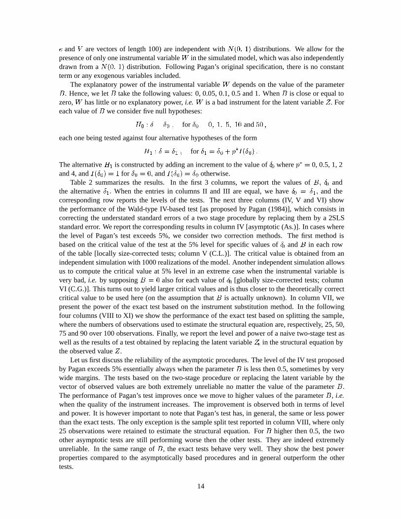
e andV are vectors of length 100) are independent withN(0; 1) distributions. We allow for thepresence of only one instrumental variableW in the simulated model, which was also independentlydrawn from aN(0; 1) distribution. Following Pagan’s original specification, there is no constantterm or any exogenous variables included.

The explanatory power of the instrumental variableW depends on the value of the parameterB. Hence, we letB take the following values: 0, 0.05, 0.1, 0.5 and 1. WhenB is close or equal tozero,W has little or no explanatory power,i.e. W is a bad instrument for the latent variableZ: Foreach value ofB we consider five null hypotheses:

H0 : Æ = Æ0 ; for Æ0 = 0; 1; 5; 10 and50 ;

each one being tested against four alternative hypotheses of the form

H1 : Æ = Æ1 ; for Æ1 = Æ0 + p�I(Æ0) :

The alternativeH1 is constructed by adding an increment to the value ofÆ0 wherep� = 0, 0.5, 1, 2and 4, andI(Æ0) = 1 for Æ0 = 0; andI(Æ0) = Æ0 otherwise.

Table 2 summarizes the results. In the first 3 columns, we report the values ofB; Æ0 andthe alternativeÆ1: When the entries in columns II and III are equal, we haveÆ0 = Æ1; and thecorresponding row reports the levels of the tests. The next three columns (IV, V and VI) showthe performance of the Wald-type IV-based test [as proposed by Pagan (1984)], which consists incorrecting the understated standard errors of a two stage procedure by replacing them by a 2SLSstandard error. We report the corresponding results in column IV [asymptotic (As.)]. In cases wherethe level of Pagan’s test exceeds 5%, we consider two correction methods. The first method isbased on the critical value of the test at the 5% level for specific values ofÆ0 andB in each rowof the table [locally size-corrected tests; column V (C.L.)]. The critical value is obtained from anindependent simulation with 1000 realizations of the model. Another independent simulation allowsus to compute the critical value at 5% level in an extreme case when the instrumental variable isvery bad,i.e. by supposingB = 0 also for each value ofÆ0 [globally size-corrected tests; columnVI (C.G.)]. This turns out to yield larger critical values and is thus closer to the theoretically correctcritical value to be used here (on the assumption thatB is actually unknown). In column VII, wepresent the power of the exact test based on the instrument substitution method. In the followingfour columns (VIII to XI) we show the performance of the exact test based on splitting the sample,where the numbers of observations used to estimate the structural equation are, respectively, 25, 50,75 and 90 over 100 observations. Finally, we report the level and power of a naive two-stage test aswell as the results of a test obtained by replacing the latent variableZ� in the structural equation bythe observed valueZ.

Let us first discuss the reliability of the asymptotic procedures. The level of the IV test proposedby Pagan exceeds 5% essentially always when the parameterB is less then 0.5, sometimes by verywide margins. The tests based on the two-stage procedure or replacing the latent variable by thevector of observed values are both extremely unreliable no matter the value of the parameterB.The performance of Pagan’s test improves once we move to higher values of the parameterB, i.e.when the quality of the instrument increases. The improvement is observed both in terms of leveland power. It is however important to note that Pagan’s test has, in general, the same or less powerthan the exact tests. The only exception is the sample split test reported in column VIII, where only25 observations were retained to estimate the structural equation. ForB higher then 0.5, the twoother asymptotic tests are still performing worse then the other tests. They are indeed extremelyunreliable. In the same range ofB, the exact tests behave very well. They show the best powerproperties compared to the asymptotically based procedures and in general outperform the othertests.

14

TABLE 2SIMULATION STUDY OF TEST PERFORMANCE FOR A MODEL

WITH UNOBSERVED REGRESSORS

Parameter Values Rejection FrequenciesB Æ0 Æ1 Wald-type IS Split-sample 2S OLS

As. C.L. C.G. 25 50 75 90I II III IV V VI VII VIII IX X XI XII XIII

0.00 0.0 0.0 0.1 � � 5.1 5.1 6.1 5.2 5.4 5.1 �

0.00 0.0 0.5 0.0 � � 4.7 5.1 4.4 4.1 3.9 4.7 �

0.00 0.0 1.0 0.0 � � 5.6 4.8 5.5 5.7 5.4 5.6 �

0.00 0.0 2.0 0.0 � � 4.2 4.5 4.5 3.8 4.5 4.2 �

0.00 0.0 4.0 0.0 � � 5.2 5.3 5.9 4.3 5.0 5.2 �

0.00 1.0 1.0 7.3 5.1 5.1 5.0 4.6 4.9 4.8 5.2 15.7 4.70.00 1.0 1.5 6.8 5.5 5.5 4.4 4.8 4.4 5.4 6.1 15.7 6.80.00 1.0 2.0 7.6 5.9 5.9 5.0 4.3 4.8 4.8 5.1 17.9 6.50.00 1.0 3.0 8.6 6.6 6.6 6.3 5.0 4.9 5.0 5.8 19.9 7.00.00 1.0 5.0 6.6 4.9 4.9 4.4 4.3 4.6 5.5 4.6 18.1 5.1

0.00 5.0 5.0 54.1 5.5 5.5 5.1 5.5 4.2 5.2 4.9 70.5 69.30.00 5.0 7.5 52.8 5.4 5.4 4.9 6.1 4.9 5.1 4.6 69.7 69.00.00 5.0 10.0 56.5 5.7 5.7 4.8 4.5 6.1 5.0 4.8 71.7 71.50.00 5.0 15.0 50.7 4.6 4.6 4.8 4.5 4.3 4.5 3.8 66.6 67.00.00 5.0 25.0 52.7 5.2 5.2 4.6 4.5 4.6 5.6 5.0 67.8 68.8

0.00 10.0 10.0 69.0 4.5 4.5 4.9 5.3 6.0 4.9 5.1 84.5 85.00.00 10.0 15.0 68.4 5.7 5.7 5.9 4.7 5.0 5.6 4.5 84.3 83.90.00 10.0 20.0 68.6 5.0 5.0 5.7 4.3 4.9 4.7 5.2 84.6 84.30.00 10.0 30.0 70.2 4.9 4.9 4.5 5.4 5.2 5.0 5.2 85.4 84.40.00 10.0 50.0 68.7 5.3 5.3 4.8 4.2 5.1 5.6 5.0 83.6 83.1

0.00 50.0 50.0 86.5 6.4 6.4 5.4 4.4 5.0 5.1 5.4 96.9 96.50.00 50.0 75.0 85.2 6.7 6.7 6.2 3.9 5.0 6.6 6.7 95.1 96.10.00 50.0 100.0 87.4 5.2 5.2 4.6 6.5 5.0 4.5 5.5 96.8 96.40.00 50.0 150.0 85.8 6.5 6.5 5.8 5.0 5.3 5.9 5.9 97.1 97.10.00 50.0 250.0 86.7 6.8 6.8 5.9 4.8 6.0 6.2 5.8 97.1 97.3

0.05 0.0 0.0 0.0 � � 4.8 5.0 3.6 3.6 5.3 4.8 �

0.05 0.0 0.5 0.2 � � 4.9 5.1 5.5 4.8 5.2 4.9 �

0.05 0.0 1.0 0.0 � � 7.4 5.4 5.7 6.2 7.6 7.4 �

0.05 0.0 2.0 0.3 � � 16.6 8.7 11.7 14.7 15.7 16.6 �

0.05 0.0 4.0 1.0 � � 47.8 16.4 26.9 38.1 44.0 47.8 �

15

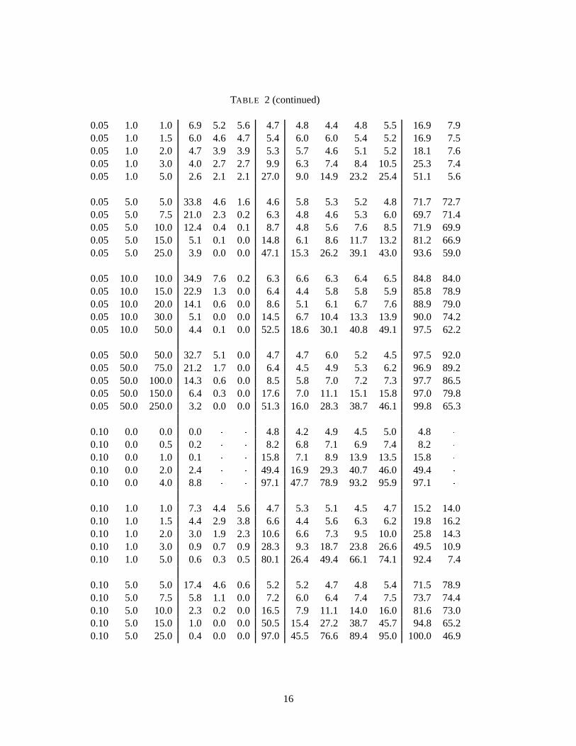
TABLE 2 (continued)

0.05 1.0 1.0 6.9 5.2 5.6 4.7 4.8 4.4 4.8 5.5 16.9 7.90.05 1.0 1.5 6.0 4.6 4.7 5.4 6.0 6.0 5.4 5.2 16.9 7.50.05 1.0 2.0 4.7 3.9 3.9 5.3 5.7 4.6 5.1 5.2 18.1 7.60.05 1.0 3.0 4.0 2.7 2.7 9.9 6.3 7.4 8.4 10.5 25.3 7.40.05 1.0 5.0 2.6 2.1 2.1 27.0 9.0 14.9 23.2 25.4 51.1 5.6

0.05 5.0 5.0 33.8 4.6 1.6 4.6 5.8 5.3 5.2 4.8 71.7 72.70.05 5.0 7.5 21.0 2.3 0.2 6.3 4.8 4.6 5.3 6.0 69.7 71.40.05 5.0 10.0 12.4 0.4 0.1 8.7 4.8 5.6 7.6 8.5 71.9 69.90.05 5.0 15.0 5.1 0.1 0.0 14.8 6.1 8.6 11.7 13.2 81.2 66.90.05 5.0 25.0 3.9 0.0 0.0 47.1 15.3 26.2 39.1 43.0 93.6 59.0

0.05 10.0 10.0 34.9 7.6 0.2 6.3 6.6 6.3 6.4 6.5 84.8 84.00.05 10.0 15.0 22.9 1.3 0.0 6.4 4.4 5.8 5.8 5.9 85.8 78.90.05 10.0 20.0 14.1 0.6 0.0 8.6 5.1 6.1 6.7 7.6 88.9 79.00.05 10.0 30.0 5.1 0.0 0.0 14.5 6.7 10.4 13.3 13.9 90.0 74.20.05 10.0 50.0 4.4 0.1 0.0 52.5 18.6 30.1 40.8 49.1 97.5 62.2

0.05 50.0 50.0 32.7 5.1 0.0 4.7 4.7 6.0 5.2 4.5 97.5 92.00.05 50.0 75.0 21.2 1.7 0.0 6.4 4.5 4.9 5.3 6.2 96.9 89.20.05 50.0 100.0 14.3 0.6 0.0 8.5 5.8 7.0 7.2 7.3 97.7 86.50.05 50.0 150.0 6.4 0.3 0.0 17.6 7.0 11.1 15.1 15.8 97.0 79.80.05 50.0 250.0 3.2 0.0 0.0 51.3 16.0 28.3 38.7 46.1 99.8 65.3

0.10 0.0 0.0 0.0 � � 4.8 4.2 4.9 4.5 5.0 4.8 �

0.10 0.0 0.5 0.2 � � 8.2 6.8 7.1 6.9 7.4 8.2 �

0.10 0.0 1.0 0.1 � � 15.8 7.1 8.9 13.9 13.5 15.8 �

0.10 0.0 2.0 2.4 � � 49.4 16.9 29.3 40.7 46.0 49.4 �

0.10 0.0 4.0 8.8 � � 97.1 47.7 78.9 93.2 95.9 97.1 �

0.10 1.0 1.0 7.3 4.4 5.6 4.7 5.3 5.1 4.5 4.7 15.2 14.00.10 1.0 1.5 4.4 2.9 3.8 6.6 4.4 5.6 6.3 6.2 19.8 16.20.10 1.0 2.0 3.0 1.9 2.3 10.6 6.6 7.3 9.5 10.0 25.8 14.30.10 1.0 3.0 0.9 0.7 0.9 28.3 9.3 18.7 23.8 26.6 49.5 10.90.10 1.0 5.0 0.6 0.3 0.5 80.1 26.4 49.4 66.1 74.1 92.4 7.4

0.10 5.0 5.0 17.4 4.6 0.6 5.2 5.2 4.7 4.8 5.4 71.5 78.90.10 5.0 7.5 5.8 1.1 0.0 7.2 6.0 6.4 7.4 7.5 73.7 74.40.10 5.0 10.0 2.3 0.2 0.0 16.5 7.9 11.1 14.0 16.0 81.6 73.00.10 5.0 15.0 1.0 0.0 0.0 50.5 15.4 27.2 38.7 45.7 94.8 65.20.10 5.0 25.0 0.4 0.0 0.0 97.0 45.5 76.6 89.4 95.0 100.0 46.9

16

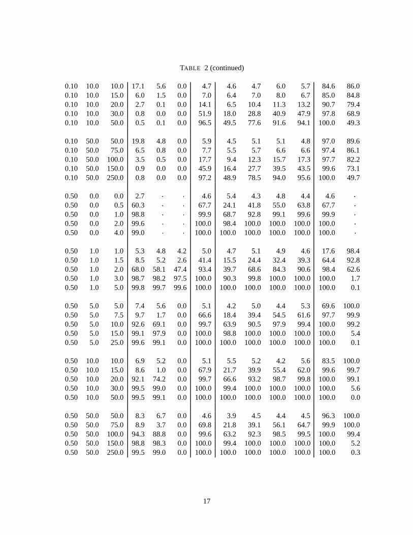
TABLE 2 (continued)

0.10 10.0 10.0 17.1 5.6 0.0 4.7 4.6 4.7 6.0 5.7 84.6 86.00.10 10.0 15.0 6.0 1.5 0.0 7.0 6.4 7.0 8.0 6.7 85.0 84.80.10 10.0 20.0 2.7 0.1 0.0 14.1 6.5 10.4 11.3 13.2 90.7 79.40.10 10.0 30.0 0.8 0.0 0.0 51.9 18.0 28.8 40.9 47.9 97.8 68.90.10 10.0 50.0 0.5 0.1 0.0 96.5 49.5 77.6 91.6 94.1 100.0 49.3

0.10 50.0 50.0 19.8 4.8 0.0 5.9 4.5 5.1 5.1 4.8 97.0 89.60.10 50.0 75.0 6.5 0.8 0.0 7.7 5.5 5.7 6.6 6.6 97.4 86.10.10 50.0 100.0 3.5 0.5 0.0 17.7 9.4 12.3 15.7 17.3 97.7 82.20.10 50.0 150.0 0.9 0.0 0.0 45.9 16.4 27.7 39.5 43.5 99.6 73.10.10 50.0 250.0 0.8 0.0 0.0 97.2 48.9 78.5 94.0 95.6 100.0 49.7

0.50 0.0 0.0 2.7 � � 4.6 5.4 4.3 4.8 4.4 4.6 �

0.50 0.0 0.5 60.3 � � 67.7 24.1 41.8 55.0 63.8 67.7 �

0.50 0.0 1.0 98.8 � � 99.9 68.7 92.8 99.1 99.6 99.9 �

0.50 0.0 2.0 99.6 � � 100.0 98.4 100.0 100.0 100.0 100.0 �

0.50 0.0 4.0 99.0 � � 100.0 100.0 100.0 100.0 100.0100.0 �

0.50 1.0 1.0 5.3 4.8 4.2 5.0 4.7 5.1 4.9 4.6 17.6 98.40.50 1.0 1.5 8.5 5.2 2.6 41.4 15.5 24.4 32.4 39.3 64.4 92.80.50 1.0 2.0 68.0 58.1 47.4 93.4 39.7 68.6 84.3 90.6 98.4 62.60.50 1.0 3.0 98.7 98.2 97.5 100.0 90.3 99.8 100.0 100.0 100.0 1.70.50 1.0 5.0 99.8 99.7 99.6 100.0 100.0 100.0 100.0 100.0100.0 0.1

0.50 5.0 5.0 7.4 5.6 0.0 5.1 4.2 5.0 4.4 5.3 69.6 100.00.50 5.0 7.5 9.7 1.7 0.0 66.6 18.4 39.4 54.5 61.6 97.7 99.90.50 5.0 10.0 92.6 69.1 0.0 99.7 63.9 90.5 97.9 99.4 100.0 99.20.50 5.0 15.0 99.1 97.9 0.0 100.0 98.8 100.0 100.0 100.0 100.0 5.40.50 5.0 25.0 99.6 99.1 0.0 100.0 100.0 100.0 100.0 100.0100.0 0.1

0.50 10.0 10.0 6.9 5.2 0.0 5.1 5.5 5.2 4.2 5.6 83.5 100.00.50 10.0 15.0 8.6 1.0 0.0 67.9 21.7 39.9 55.4 62.0 99.6 99.70.50 10.0 20.0 92.1 74.2 0.0 99.7 66.6 93.2 98.7 99.8 100.0 99.10.50 10.0 30.0 99.5 99.0 0.0 100.0 99.4 100.0 100.0 100.0 100.0 5.60.50 10.0 50.0 99.5 99.1 0.0 100.0 100.0 100.0 100.0 100.0100.0 0.0

0.50 50.0 50.0 8.3 6.7 0.0 4.6 3.9 4.5 4.4 4.5 96.3 100.00.50 50.0 75.0 8.9 3.7 0.0 69.8 21.8 39.1 56.1 64.7 99.9 100.00.50 50.0 100.0 94.3 88.8 0.0 99.6 63.2 92.3 98.5 99.5 100.0 99.40.50 50.0 150.0 98.8 98.3 0.0 100.0 99.4 100.0 100.0 100.0 100.0 5.20.50 50.0 250.0 99.5 99.0 0.0 100.0 100.0 100.0 100.0 100.0100.0 0.3

17

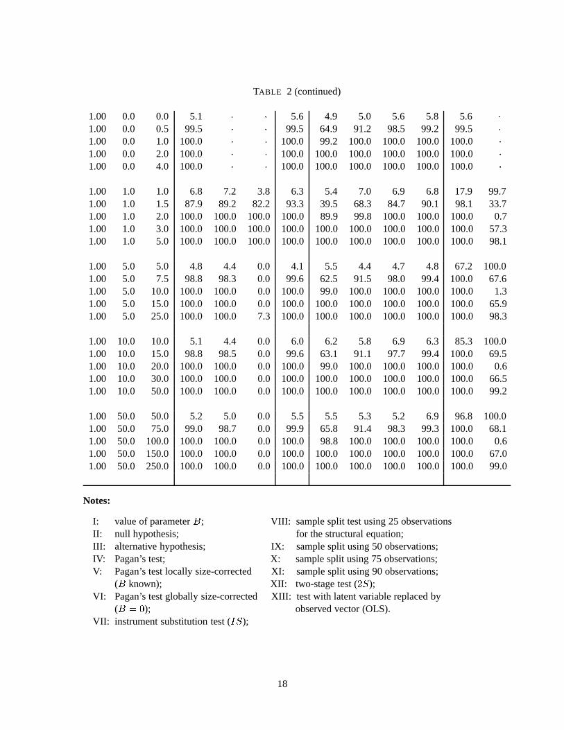
TABLE 2 (continued)

1.00 0.0 0.0 5.1 � � 5.6 4.9 5.0 5.6 5.8 5.6 �

1.00 0.0 0.5 99.5 � � 99.5 64.9 91.2 98.5 99.2 99.5 �

1.00 0.0 1.0 100.0 � � 100.0 99.2 100.0 100.0 100.0 100.0 �

1.00 0.0 2.0 100.0 � � 100.0 100.0 100.0 100.0 100.0100.0 �

1.00 0.0 4.0 100.0 � � 100.0 100.0 100.0 100.0 100.0100.0 �

1.00 1.0 1.0 6.8 7.2 3.8 6.3 5.4 7.0 6.9 6.8 17.9 99.71.00 1.0 1.5 87.9 89.2 82.2 93.3 39.5 68.3 84.7 90.1 98.1 33.71.00 1.0 2.0 100.0 100.0 100.0 100.0 89.9 99.8 100.0 100.0 100.0 0.71.00 1.0 3.0 100.0 100.0 100.0 100.0 100.0 100.0 100.0 100.0100.0 57.31.00 1.0 5.0 100.0 100.0 100.0 100.0 100.0 100.0 100.0 100.0100.0 98.1

1.00 5.0 5.0 4.8 4.4 0.0 4.1 5.5 4.4 4.7 4.8 67.2 100.01.00 5.0 7.5 98.8 98.3 0.0 99.6 62.5 91.5 98.0 99.4 100.0 67.61.00 5.0 10.0 100.0 100.0 0.0 100.0 99.0 100.0 100.0 100.0 100.0 1.31.00 5.0 15.0 100.0 100.0 0.0 100.0 100.0 100.0 100.0 100.0100.0 65.91.00 5.0 25.0 100.0 100.0 7.3 100.0 100.0 100.0 100.0 100.0100.0 98.3

1.00 10.0 10.0 5.1 4.4 0.0 6.0 6.2 5.8 6.9 6.3 85.3 100.01.00 10.0 15.0 98.8 98.5 0.0 99.6 63.1 91.1 97.7 99.4 100.0 69.51.00 10.0 20.0 100.0 100.0 0.0 100.0 99.0 100.0 100.0 100.0 100.0 0.61.00 10.0 30.0 100.0 100.0 0.0 100.0 100.0 100.0 100.0 100.0100.0 66.51.00 10.0 50.0 100.0 100.0 0.0 100.0 100.0 100.0 100.0 100.0100.0 99.2

1.00 50.0 50.0 5.2 5.0 0.0 5.5 5.5 5.3 5.2 6.9 96.8 100.01.00 50.0 75.0 99.0 98.7 0.0 99.9 65.8 91.4 98.3 99.3 100.0 68.11.00 50.0 100.0 100.0 100.0 0.0 100.0 98.8 100.0 100.0 100.0 100.0 0.61.00 50.0 150.0 100.0 100.0 0.0 100.0 100.0 100.0 100.0 100.0100.0 67.01.00 50.0 250.0 100.0 100.0 0.0 100.0 100.0 100.0 100.0 100.0100.0 99.0

Notes:

I: value of parameterB; VIII: sample split test using 25 observationsII: null hypothesis; for the structural equation;III: alternative hypothesis; IX: sample split using 50 observations;IV: Pagan’s test; X: sample split using 75 observations;V: Pagan’s test locally size-corrected XI: sample split using 90 observations;

(B known); XII: two-stage test (2S);VI: Pagan’s test globally size-corrected XIII: test with latent variable replaced by

(B = 0); observed vector (OLS).VII: instrument substitution test (IS);

18

9 Empirical illustrations

In this section, we present empirical results on inference in two distinct economic models with latentregressors. The first example is based on Tobin’s marginalq model of investment (Tobin, 1969),with fixed assets used as the instrumental variable forq. The second model stems from educationaleconomics and relates students’ academic achievements to a number of personal characteristics andother socioeconomic variables. Among the personal characteristics, we encounter a variable definedas “self–esteem” which is viewed as an imperfect measure of a latent variable and is instrumentedby measures of the prestige of parents’ professional occupation. The first example is one where wehave good instruments, while the opposite holds for the second example.

Consider first Tobin’s marginalq model of investment (Tobin, 1969). Investment of an indi-vidual firm is defined as an increasing function of the shadow value of capital, equal to the presentdiscounted value of expected marginal profits. In Tobin’s original setup, investment behavior of allfirms is similar and no difference arises from the degree of availability of external financing. In fact,investment behavior varies across firms and is determined to a large extent by financial constraintssome firms are facing in the presence of asymmetric information. For those firms, external financ-ing may either be too costly or not provided for other reasons. Thus investment depends heavily onthe firm’s own source of financing, namely the cash flow. To account for differences in investmentbehavior implied by financial constraints, several authors [Abel (1979), Hayashi (1985), Abel andBlanchard (1986), Abel and Eberly (1993)] introduced the cash flow as an additional regressor toTobin’s q model. It can be argued that another explanatory variable controlling the profitability ofinvestment is also required. For this reason, one can argue that the firm’s income has to be includedin the investment regression as well. The model is thus

Ii = 0 + ÆQi + 1CFi + 2Ri + ei(9.1)

whereIi denotes the investment expenses of an individual firmi, CFi andRi its cash flow andincome respectively, whileQi is Tobin’sq measured by equity plus debt and approximated empir-ically by adding data on current debt, long term debt, deferred taxes and credit, minority interestand equity less inventory;Æ and = ( 0; 1; 2)

0 are fixed coefficients to be estimated. Given thecompound character ofQi; which is constructed from several indexes, fixed assets are used as anexplanatory variable forQi in the regression which completes the model:

Qi = �0 + �1Fi + vi :(9.2)

For the purpose of building finite-sample confidence intervals following the instrument substitutionmethod, the latter equation may be replaced (without any change to the results) by the more generalequation (called below the “full instrumental regression”):

Qi = �0 + �1Fi + �3CFi + �4Ri + vi :(9.3)

Our empirical work is based on “Stock Guide Database” containing data on companies listedat the Toronto and Montreal stock exchange markets between 1987 and 1991. The records consistof observations on economic variables describing the firms’ size and performance, like fixed capitalstock, income, cash flow, stock market price, etc. All data on the individual companies have previ-ously been extracted from their annual, interim and other reports. We retained a subsample of 9285firms whose stocks were traded on the Toronto and Montreal stock exchange markets in 1991.

Since we are interested in comparing our inference methods to the widely used Wald-type tests,we first consider the approach suggested by Pagan (1984). Since usual estimators of coefficient

19

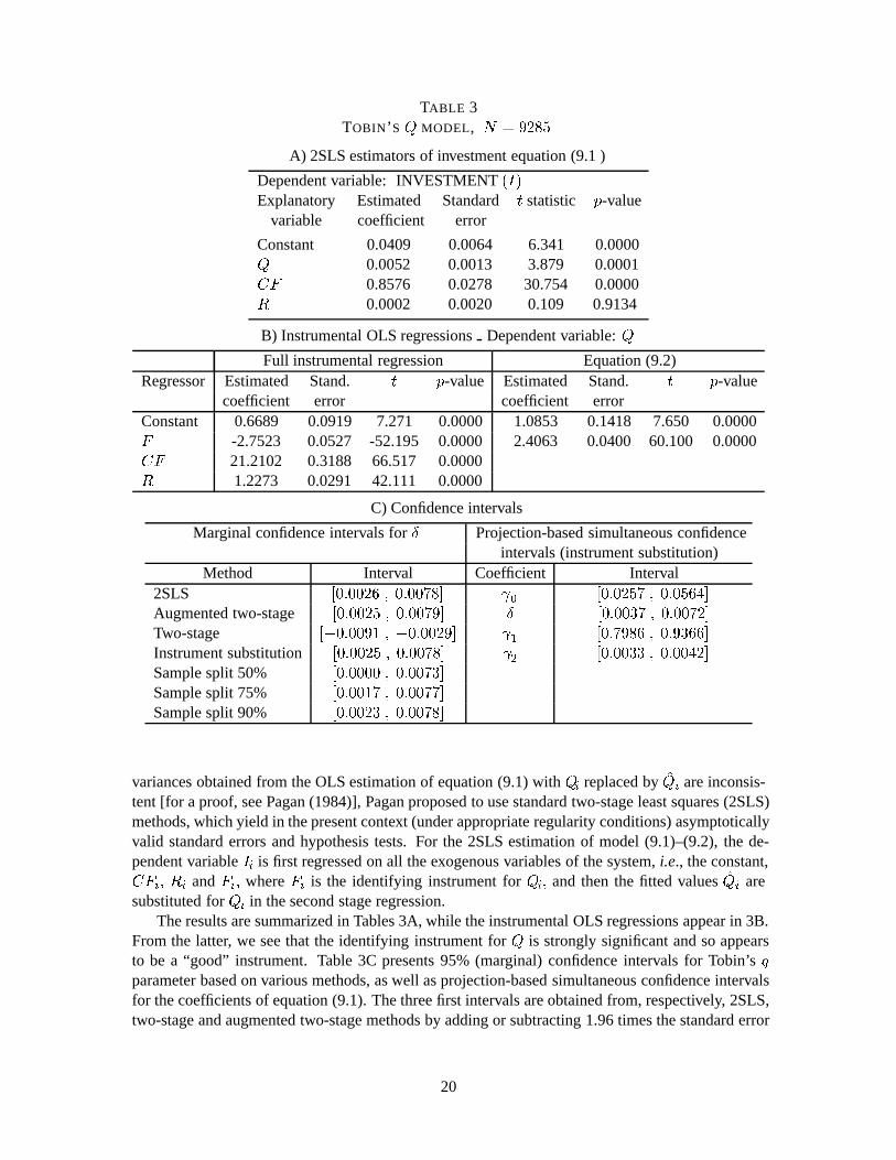
TABLE 3TOBIN’ S Q MODEL, N = 9285

A) 2SLS estimators of investment equation (9.1 )

Dependent variable: INVESTMENT(I)Explanatory Estimated Standardt statistic p-value

variable coefficient error

Constant 0.0409 0.0064 6.341 0.0000Q 0.0052 0.0013 3.879 0.0001CF 0.8576 0.0278 30.754 0.0000R 0.0002 0.0020 0.109 0.9134

B) Instrumental OLS regressionsDependent variable:Q

Full instrumental regression Equation (9.2)Regressor Estimated Stand. t p-value Estimated Stand. t p-value

coefficient error coefficient errorConstant 0.6689 0.0919 7.271 0.0000 1.0853 0.1418 7.650 0.0000F -2.7523 0.0527 -52.195 0.0000 2.4063 0.0400 60.100 0.0000CF 21.2102 0.3188 66.517 0.0000R 1.2273 0.0291 42.111 0.0000

C) Confidence intervals

Marginal confidence intervals forÆ Projection-based simultaneous confidenceintervals (instrument substitution)

Method Interval Coefficient Interval2SLS [0:0026 ; 0:0078] 0 [0:0257 ; 0:0564]

Augmented two-stage [0:0025 ; 0:0079] Æ [0:0037 ; 0:0072]

Two-stage [�0:0091 ; �0:0029] 1 [0:7986 ; 0:9366]

Instrument substitution [0:0025 ; 0:0078] 2 [0:0033 ; 0:0042]

Sample split 50% [0:0000 ; 0:0073]

Sample split 75% [0:0017 ; 0:0077]

Sample split 90% [0:0023 ; 0:0078]

variances obtained from the OLS estimation of equation (9.1) withQi replaced byQi are inconsis-tent [for a proof, see Pagan (1984)], Pagan proposed to use standard two-stage least squares (2SLS)methods, which yield in the present context (under appropriate regularity conditions) asymptoticallyvalid standard errors and hypothesis tests. For the 2SLS estimation of model (9.1)–(9.2), the de-pendent variableIi is first regressed on all the exogenous variables of the system,i.e., the constant,CFi; Ri andFi; whereFi is the identifying instrument forQi; and then the fitted valuesQi aresubstituted forQi in the second stage regression.

The results are summarized in Tables 3A, while the instrumental OLS regressions appear in 3B.From the latter, we see that the identifying instrument forQ is strongly significant and so appearsto be a “good” instrument. Table 3C presents 95% (marginal) confidence intervals for Tobin’sq

parameter based on various methods, as well as projection-based simultaneous confidence intervalsfor the coefficients of equation (9.1). The three first intervals are obtained from, respectively, 2SLS,two-stage and augmented two-stage methods by adding or subtracting 1.96 times the standard error

20

to/from the estimated parameter value.1 Below we report the exact confidence intervals (instrumentsubstitution and sample split) based on the solution of quadratic equations as described in Sections2 and 3. Recall that the precision of the confidence intervals depends, in the case of the samplesplit method, on the number of observations retained for the estimation of the structural equation.We thus show the results for, respectively, 50%, 75% and 90% of the entire sample (selected ran-domly). The simultaneous confidence intervals for the elements of the vector� = ( 0; Æ; 1; 2)

0

are obtained by first building a simultaneous confidence setC�(�), with level 1 � � = 0:95 for �according to the instrument substitution method described in Section 4 and then by both minimizingand maximizing each coefficient subject to the restriction� 2 C�(�) [see Section 6]. The programused to perform these constrained optimizations is the subroutine NCONF from the IMSL math-ematical library. The corresponding four-dimensional confidence box has level95% (or possiblymore),i.e: we have simultaneous confidence intervals (at level95%):

From these results, we see that all the confidence intervals forÆ; except for the two-stage interval(which is not asymptotically valid), are quite close to each other. Among the finite-sample intervals,the ones based on the instrument substitution and the 90% sample split method appear to be the mostprecise. It is also worthwhile noting that the projection-based simultaneous confidence intervals allappear to be quite short. This shows that the latter method works well in the present context and canbe implemented easily.

Let us now consider another example where, on the contrary, important discrepancies arisebetween the intervals based on the asymptotic and the exact inference methods. Montmarquetteand Mahseredjian (Montmarquette and Mahseredjian, 1989; Montmarquette, Houle, Crespo andMahseredjian, 1989) studied students’ academic achievements as a function of personal and socioe-conomic explanatory variables. Students’ school results in French and mathematics are measuredby the grade, taking values on the interval0 � 100: The grade variable is assumed to depend onpersonal characteristics, such as age, intellectual ability (IQ) observed in kindergarten and “self–esteem” measured on an adapted children self–esteem scale ranging from 0 to 40. Other explanatoryvariables include parents’ income, father’s and mother’s education measured in number of years ofschooling, the number of siblings, student’s absenteeism, his own education and experience as wellas the class size. We examine the significance of self–esteem, which is viewed as an imperfectlymeasured latent variable to explain the first grader’s achievements in mathematics. The self esteemof younger children was measured by a French adaptation of the McDaniel–Piers scale. Noting themeasurement scale may not be equally well adjusted to the age of all students and due to the highdegree of arbitrariness in the choice of this criterion, the latter was instrumented by Blishen indicesreflecting the prestige of father’s and mother’s professional occupations in order to take account ofeventual mismeasurement.

The data stem from a 1981–1982 survey of first graders attending Montreal francophone publicelementary schools. The sample consists of 603 observations on students’ achievements in mathe-matics. The model considered is:

LMATi = �0 + Æ SEi + �1 IQi + �2 Ii + �3 FEi + �4MEi + �5 SNi

+ �6Ai + �7ABPi + �8 EXi + �9EDi + �10ABSi + �11 CSi + ei

(9.4)

where (for each individuali) LMAT = `n(grade/(100� grade)),SE = `n(self esteem test re-sult/(40� self esteem test result)),IQ is a measure of intelligence (observed in kindergarten),I is

1The augmented two-stage method uses all the available instruments to compute the generated regressors (full in-strumental regression), rather than the restricted instrumental equation (9.2). As with the two-stage method, OLS-basedcoefficient standard errors obtained in this way are inconsistent; see Pagan (1984) for further discussion.

21

parents’ income,FE andME are father’s and mother’s years of schooling,SN denotes the sibling’snumber,A is the age of the student,ABP is a measure of teacher’s absenteeism,EX indicates theyears of student’s work experience,ED measures his education in years,ABS is student’s absen-teeism andCS denotes the class size. Finally, the instrumental regression is:

SEi = 0 + 1 FPi + 2MPi + vi(9.5)

whereFP andMP correspond to the prestige of the father and mother’s profession expressed interms of Blishen indices. We consider also the more general instrumental regression which includesall the explanatory variables on the right-hand side of (9.4) exceptSE: The 2SLS estimates andprojection-based simultaneous confidence are reported in Table 4A while the results of the instru-mental regressions appear in Table 4B.

Standard (bounded) Wald-type confidence intervals are of course entailed by the 2SLS estima-tion. ForÆ however, the instrument substitution method yields the confidence interval defined bythe inequality:�31:9536 Æ20 � 84:7320 Æ0 � 850:9727 � 0 : Since the roots of this second orderpolynomial are complex anda < 0; this confidence interval actually covers the whole real line.Indeed, from the full instrumental regression and usingt-tests as well as the relevantF -test (Table4B), we see that the coefficients ofFP andMP are not significantly different from zero,i.e. thelatter appear to be poor instruments. So the fact that we get here an unbounded confidence intervalfor Æ is expected in the light of the remarks at the end of Section 2. The projection-based confidenceintervals (Table 4A) yield the same message forÆ; although it is of interest to note that the intervalsfor the other coefficients of the model can be quite short despite the fact thatÆ may be difficult toidentify. As in the case of multicollinearity problems in linear regressions, inference about somecoefficients of a model remains feasible even if the certain parameters are not identifiable.

10 Conclusions

The inference methods presented in this paper are applicable to a variety of models, such as re-gressions with unobserved explanatory variables or structural models which can be estimated byinstrumental variable methods (e.g., simultaneous equations models). They may be considered asextensions of Anderson-Rubin procedures where the major improvement consists of providing testsof hypotheses on subsets or elements of the parameter vector. This is accomplished via a projectiontechnique allowing for inference on general possibly nonlinear transformations of the parametervector of interest. We emphasized that our test statistics, being pivotal or at least boundedly pivotalfunctions, yield valid confidence sets which are unbounded with a non-zero probability. The un-boundedness of confidence sets is of particular importance when the instruments are poor and theparameter of interest is not identifiable or close to being unidentified. Accordingly, a valid confi-dence set should cover the entire set of real numbers since all values are observationally equivalent[see Dufour (1997) and Gleser and Hwang (1987)]. Our empirical results indicate that inferencemethods based on Wald-type statistics are unreliable in the presence of poor instruments since suchmethods typically yield bounded confidence sets with probability one. The results in this paperthus underscore another shortcoming of Wald-type procedures which is quite distinct from otherproblematic properties, such as non-invariance to reparameterizations [see Dagenais and Dufour(1991)].

In general, non-identifiability of parameters results either from low quality instruments or, morefundamentally, from a poor model specification. A valid test yielding an unbounded confidenceset becomes thus a relevant indicator of problems involving the econometric setup. The powerproperties of exact and Wald-type tests were compared in a simulation-based experiment. The test

22

TABLE 4MATHEMATICS ACHIEVEMENT MODEL N = 603

2SLS estimators of achievement equation (9.4) Projection-basedDependent variable: LMAT 95% confidence intervalsExplanatory Estimated Standardt statistic p-value (instrument substitution)

variable coefficient errorConstant -4.1557 0.9959 -4.173 0.0000 [-4.8601 , -3.7411]SE 0.2316 0.3813 0.607 0.5438 (�1;+1)

IQ 0.0067 0.0015 4.203 0.0000 [0.006600 , 0.006724]I 0.0002 0.3175 0.008 0.9939 [-0.09123 , 0.10490]FE 0.0015 0.0089 0.172 0.8636 [-0.00914 , 0.01889]ME 0.0393 0.0117 3.342 0.0009 [0.02868 , 0.05762]SN -0.0008 0.0294 -0.029 0.9767 [-0.1546 , 0.1891]A 0.0144 0.0070 2.050 0.0408 [0.01272 , 0.01877]ABP -0.0008 0.0005 -1.425 0.1548 [-0.003778 , 0.000865]EX -0.0056 0.0039 -1.420 0.1561 [-0.01307 , 0.00333]ED -0.0007 0.0206 -0.035 0.9718 [-0.0123 , 0.2196]ABS -0.0001 0.0002 -0.520 0.6033[-0.0001764 , 0.0000786]CS -0.0184 0.0093 -1.964 0.0500 [-0.03003 , -0.009790]

Marginal95% quadratic confidence interval forÆ (�1;+1)

Instrumental OLS regressionsDependent variable: SE

Full instrumental regression Equation (9.5)Regressor Estimated Stand. t p-value Estimated Stand. t p-value

coefficient error coefficient errorConstant -1.2572 1.0511 -1.1960 0.232 0.8117 0.1188 6.830 0.0000FP 0.5405 0.3180 1.7000 0.090 0.5120 0.2625 1.951 0.0516FM 0.3994 0.3327 1.2004 0.230 0.6170 0.2811 2.194 0.0286IQ 0.003822 0.000611 6.2593 0.000I 0.02860 0.03161 0.9049 0.366 F -statistic for significance of FP andFE -0.01352 0.01136 -1.1899 0.235 FM in full instrumental regression:ME -0.004028 0.01517 -0.2655 0.791 F (2; 589) = 2:654 (p-value= 0.078)SN -0.01439 0.03325 -0.4326 0.665A 0.003216 0.008161 0.3941 0.694ABP 0.000698 0.000577 1.2108 0.226EX -0.002644 0.004466 -0.5920 0.554ED -0.02936 0.02080 -1.4117 0.159ABS 0.000426 0.000194 2.1926 0.029CS 0.01148 0.009595 1.1966 0.232

23

performances were examined by simulations on a simple model with varying levels of instrumentquality and the extent to which the null hypotheses differ from the true parameter value. We foundthat the tests proposed in this paper were preferable to more usual IV-based Wald-type methods fromthe points of view of level control and power. This seems to occur despite the fact that AR-type pro-cedures involve “projections onto a high-dimensional subspace which could result in reduced powerand thus wide confidence regions” [Staiger and Stock (1997, p. 570)]. However, it is important toremember that size-correcting Wald-type procedures requires one to use huge critical values thatcan easily destroy power. Wald-type procedures can be made useful only at the cost introducing im-portant and complex restrictions on the parameter space that one is not generally prepare to impose;for further discussion of these difficulties, see Dufour (1997, Section 6).

It is important to note that although the simulations were performed under the normality as-sumption, our tests yield valid inferences in more general cases involving non-Gaussian errors andweakly exogenous instruments. This result has a theoretical justification and is also confirmed byour empirical examples. Since the inference methods we propose are as well computationally easyto perform, they can be considered as a reliable and a powerful alternative to more usual Wald-typeprocedures.

References

ABEL, A. (1979): Investment and the Value of Capital. New York: Garland Publishing.ABEL, A. AND O. J. BLANCHARD (1986): “The Present Value of Profits and Cyclical Movements

in Investment,”Econometrica, 54, 249–273.ABEL, A. AND J. EBERLY (1993): “A Unified Model of Investment under Uncertainty,” Technical

Report 4296, National Bureau of Economic Research, Cambridge, MA.ANDERSON, T. W. AND H. RUBIN (1949): “Estimation of the Parameters of a Single Equation in

a Complete System of Stochastic Equations,”Annals of Mathematical Statistics, 20, 46–63.ANGRIST, J. D. AND A. B. KRUEGER (1994): “Split Sample Instrumental Variables,” Technical

Working Paper 150, N.B.E.R., Cambridge, MA.BARRO, R. J. (1977): “Unanticipated Money Growth and Unemployment in the United States,”

American Economic Review, 67, 101–115.BATES, D. M. AND D. G. WATTS (1988): Nonlinear Regression Analysis and its Applications.

New York: John Wiley & Sons.BOUND, J., D. A. JAEGER, AND R. BAKER (1993): “The Cure can be Worse than the Disease:

A Cautionary Tale Regarding Instrumental Variables,” Technical Working Paper 137, NationalBureau of Economic Research, Cambridge, MA.

BOUND, J., D. A. JAEGER, AND R. M. BAKER (1995): “Problems With Instrumental VariablesEstimation When the Correlation Between the Instruments and the Endogenous Explanatory Vari-able Is Weak,”Journal of the American Statistical Association, 90, 443–450.

BUSE, A. (1992): “The Bias of Instrumental Variables Estimators,”Econometrica, 60, 173–180.CHEN, J.-S.AND R. I. JENNRICH (1996): “The Signed Root Deviance Profile and Confidence

Intervals in Maximum Likelihood Analysis,”Journal of the American Statistical Association, 91,993–999.

DAGENAIS, M. G. AND J.-M. DUFOUR (1991): “Invariance, Nonlinear Models and AsymptoticTests,”Econometrica, 59, 1601–1615.

DUFOUR, J.-M. (1989): “Nonlinear Hypotheses, Inequality Restrictions, and Non-Nested Hy-potheses: Exact Simultaneous Tests in Linear Regressions,”Econometrica, 57, 335–355.

(1990): “Exact Tests and Confidence Sets in Linear Regressions with Autocorrelated Errors,”

24

Econometrica, 58, 475–494.(1997): “Some Impossibility Theorems in Econometrics, with Applications to Structural and

Dynamic Models,”Econometrica, 65, 1365–1389.DUFOUR, J.-M. AND J. JASIAK (1993): “Finite Sample Inference Methods for Simultaneous Equa-

tions and Models with Unobserved and Generated Regressors,” Technical report, C.R.D.E., Uni-versite de Montreal.

DUFOUR, J.-M. AND J. F. KIVIET (1996): “Exact Tests for Structural Change in First-Order Dy-namic Models,”Journal of Econometrics, 70, 39–68.

(1998): “Exact Inference Methods for First-Order Autoregressive Distributed Lag Models,”Econometrica, 66, 79–104.

DUFOUR, J.-M. AND O. TORRES (1998): “Union-Intersection and Sample-Split Methods inEconometrics with Applications to SURE and MA Models,” inHandbook of Applied EconomicStatistics, ed. by D. E. A. Giles and A. Ullah. New York: Marcel Dekker, pp. 465–505.

FULLER, W. A. (1987):Measurement Error Models. New York: John Wiley & Sons.GLESER, L. J. AND J. T. HWANG (1987): “The Nonexistence of100(1 � �) Confidence Sets of

Finite Expected Diameter in Errors in Variables and Related Models,”The Annals of Statistics,15, 1351–1362.

HALL , A. R., G. D. RUDEBUSCH, AND D. W. WILCOX (1996): “Judging Instrument Relevancein Instrumental Variables Estimation,”International Economic Review, 37, 283–298.

HAYASHI , F. (1982): “Tobin’s Marginalq and Averageq: A Neoclassical Interpretation,”Econo-metrica, 50, 213–224.

KIVIET, J.AND J.-M. DUFOUR(1997): “Exact Tests in Single Equation Autoregressive DistributedLag Models,”Journal of Econometrics, 80, 325–353.

MADDALA , G. S. (1974): “Some Small Sample Evidence on Tests of Significance in SimultaneousEquations Models,”Econometrica, 42, 841–851.

MADDALA , G. S.AND J. JEONG (1992): “On the Exact Small Sample Distribution of the Instru-mental Variable Estimator,”Econometrica, 60, 181–183.

MEEKER, W. Q.AND L. A. ESCOBAR(1995): “Teaching About Approximate Confidence RegionsBased on Maximum Likelihood Estimation,”The American Statistician, 49, 48–53.

MILLER, R. G., JR. (1981): Simultaneous Statistical Inference (Second Edition). New York:Springer-Verlag.

MONTMARQUETTE, C., R. HOULE, M. CRESPO, AND S. MAHSEREDJIAN (1989): Les inter-ventions scolaires en milieu defavorise: estimation et evaluation. Montreal: Les Presses del’Universite de Montreal.

MONTMARQUETTE, C. AND S. MAHSEREDJIAN (1989): “Could Teacher Grading Practices Ac-count for Unexplained Variation in School Achievements?,”Economics of Education Review, 8,335–343.

MURPHY, K. M. AND R. H. TOPEL (1985): “Estimation and Inference in Two-Step EconometricModels,”Journal of Business and Economic Statistics, 3, 370–379.

NAGAR, A. L. (1959): “The Bias and Moment Matrix of the General k-class Estimators of theParameters in Simultaneous Equations,”Econometrica, 27, 575–595.

NELSON, C. R.AND R. STARTZ (1990a): “The Distribution of the Instrumental Variable Estimatorand itst-ratio When the Instrument is a Poor One,”Journal of Business, 63, 125–140.

(1990b): “Some Further Results on the Exact Small Properties of the Instrumental VariableEstimator,”Econometrica, 58, 967–976.

OXLEY, L. AND M. M CALEER (1993): “Econometric Issues in Macroeconomic Models with Gen-erated Regressors,”Journal of Economic Surveys, 7, 1–39.

PAGAN, A. (1984): “Econometric Issues in the Analysis of Regressions with Generated Regres-

25

sors,”International Economic Review, 25, 221–247.(1986): “Two Stage and Related Estimators and their Applications,”Review of Economic Stud-

ies, 53, 517–538.RICHARDSON, D. H. (1968): “The Exact Distribution of a Structural Coefficient Estimator,”Jour-

nal of the American Statistical Association, 63, 1214–1226.SAVIN , N. E. (1984): “Multiple Hypothesis Testing,” inHandbook of Econometrics, Volume 2, ed.

by Z. Griliches and M. D. Intrilligator. Amsterdam: North-Holland, pp. 827–879.SAWA , T. (1969): “The Exact Sampling Distribution of Ordinary Least Squares and Two-Stage

Least Squares Estimators,”Journal of the American Statistical Association, 64, 923–937.STAIGER, D. AND J. H. STOCK (1997): “Instrumental Variables Regression with Weak Instru-

ments,”Econometrica, 65, 557–586.

26