Finite Element Model for Atmospheric IR-Absorption · Finite element model for the IR absorption in...
18
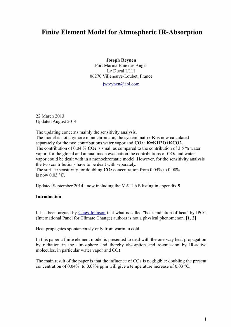
Finite Element Model for Atmospheric IR-Absorption Joseph Reynen Port Marina Baie des Anges Le Ducal U111 06270 Villeneuve-Loubet, France [email protected] 22 March 2013 Updated August 2014 The updating concerns mainly the sensitivity analysis. The model is not anymore monochromatic, the system matrix K is now calculated separately for the two contributions water vapor and CO2 : K=KH2O+KCO2. The contribution of 0.04 % CO2 is small as compared to the contribution of 3.5 % water vapor: for the global and annual mean evacuation the contributions of CO2 and water vapor could be dealt with in a monochromatic model. However, for the sensitivity analysis the two contributions have to be dealt with separately. The surface sensitivity for doubling CO2 concentration from 0.04% to 0.08% is now 0.03 °C. Updated September 2014 . now including the MATLAB listing in appendix 5 Introduction It has been argued by Claes Johnson that what is called "back-radiation of heat" by IPCC (International Panel for Climate Change) authors is not a physical phenomenon. [1, 2] Heat propagates spontaneously only from warm to cold. In this paper a finite element model is presented to deal with the one-way heat propagation by radiation in the atmosphere and thereby absorption and re-emission by IR-active molecules, in particular water vapor and CO2. The main result of the paper is that the influence of CO 2 is negligible: doubling the present concentration of 0.04% to 0.08% ppm will give a temperature increase of 0.03 °C. 1
Transcript of Finite Element Model for Atmospheric IR-Absorption · Finite element model for the IR absorption in...
Finite Element Model for Atmospheric IR-Absorption
Joseph ReynenPort Marina Baie des Anges
Le Ducal U11106270 Villeneuve-Loubet, France
22 March 2013Updated August 2014
The updating concerns mainly the sensitivity analysis.The model is not anymore monochromatic, the system matrix K is now calculated separately for the two contributions water vapor and CO2 : K=KH2O+KCO2.The contribution of 0.04 % CO2 is small as compared to the contribution of 3.5 % water vapor: for the global and annual mean evacuation the contributions of CO2 and water vapor could be dealt with in a monochromatic model. However, for the sensitivity analysis the two contributions have to be dealt with separately.The surface sensitivity for doubling CO2 concentration from 0.04% to 0.08% is now 0.03 °C.
Updated September 2014 . now including the MATLAB listing in appendix 5
Introduction
It has been argued by Claes Johnson that what is called "back-radiation of heat" by IPCC(International Panel for Climate Change) authors is not a physical phenomenon. [1, 2]
Heat propagates spontaneously only from warm to cold.
In this paper a finite element model is presented to deal with the one-way heat propagationby radiation in the atmosphere and thereby absorption and re-emission by IR-activemolecules, in particular water vapor and CO2.
The main result of the paper is that the influence of CO2 is negligible: doubling the presentconcentration of 0.04% to 0.08% ppm will give a temperature increase of 0.03 °C.
1
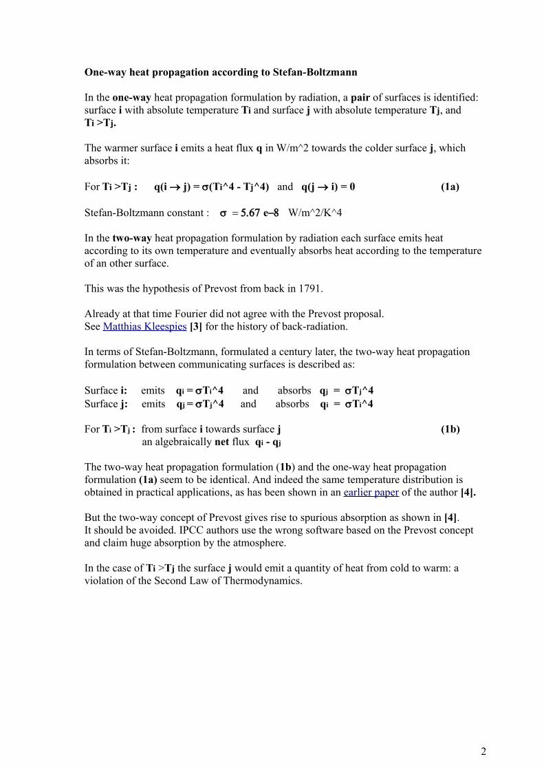
One-way heat propagation according to Stefan-Boltzmann
In the one-way heat propagation formulation by radiation, a pair of surfaces is identified: surface i with absolute temperature Ti and surface j with absolute temperature Tj, and Ti >Tj.
The warmer surface i emits a heat flux q in W/m^2 towards the colder surface j, which absorbs it:
For Ti >Tj : q(i j) = (Ti^4 - Tj^4) and q(j i) = 0 (1a)
Stefan-Boltzmann constant : eW/m^2/K^4
In the two-way heat propagation formulation by radiation each surface emits heat according to its own temperature and eventually absorbs heat according to the temperature of an other surface.
This was the hypothesis of Prevost from back in 1791.
Already at that time Fourier did not agree with the Prevost proposal.See Matthias Kleespies [3] for the history of back-radiation.
In terms of Stefan-Boltzmann, formulated a century later, the two-way heat propagation formulation between communicating surfaces is described as: Surface i: emits qi = Ti^4 and absorbs qj = Tj^4 Surface j: emits qj = Tj^4 and absorbs qi = Ti^4
For Ti >Tj : from surface i towards surface j (1b) an algebraically net flux qi - qj
The two-way heat propagation formulation (1b) and the one-way heat propagation formulation (1a) seem to be identical. And indeed the same temperature distribution is obtained in practical applications, as has been shown in an earlier paper of the author [4].
But the two-way concept of Prevost gives rise to spurious absorption as shown in [4].It should be avoided. IPCC authors use the wrong software based on the Prevost concept and claim huge absorption by the atmosphere.
In the case of Ti >Tj the surface j would emit a quantity of heat from cold to warm: a violation of the Second Law of Thermodynamics.
2

Finite element model for the IR absorption in the atmosphere
We will derive in this section a set of simultaneous linear equations for heat radiation in a multilayer semi-transparent stack according to the one-way heat propagation formulation, using the finite element method (FEM).
It is an amelioration of an earlier finite difference model [4]. We model the semi-transparent atmosphere as a stack of N-2 grids consisting of fully transparent holes and fully absorbing wires with a normalized cross-section (1-fi ) and fi , respectively. Such a grid can be considered as a very fine gauze.
The lower level of the stack at node 1 represents the surface of the planet, outer-space is represented by node N.
To each node i of the stack a temperatures Ti is allocated, converted into variables θi=σTi^4.The dimension of these variables is W/m^2 and indeed θ, although variables related to temperature, sometimes represent heat fluxes. It follows from the context.
The wires of a grid in the stack exchange heat by radiation with the wires of other grids in the stack according to equation (1a), the one-way heat propagation formulation of the SB law, from the warmer ones to the colder ones, according to the Second Law of Thermodynamics.
In transverse direction i.e. parallel to the surface of the planet, the dimensions are supposedto be infinitely large: by symmetry only heat propagation by radiation in vertical direction has to be considered.
The dimensionless cross-section fi of the wire i.e. the diameter of the wire multiplied by its length per unit of area of the gauze, can vary for the various grids in vertical direction and can be interpreted as an absorption/emission coefficient. It will be called as such from now on.
We consider the one-way heat radiation between two layers i and j by LW radiation according to the SB law (1a), as depicted by the basic radiation finite element in Figure 1.
Figure 1 Basic finite element for heat radiation between grids i and j.
qj → — — — — — — — — — — — — — fj, θj
element heat flux↑fe*(θi-θj)
qi → — — — — — — — — — — — — — fi, θi
Grids i and j are not necessarily adjacent, other grids can be in between.
The nodal parameters are:
3
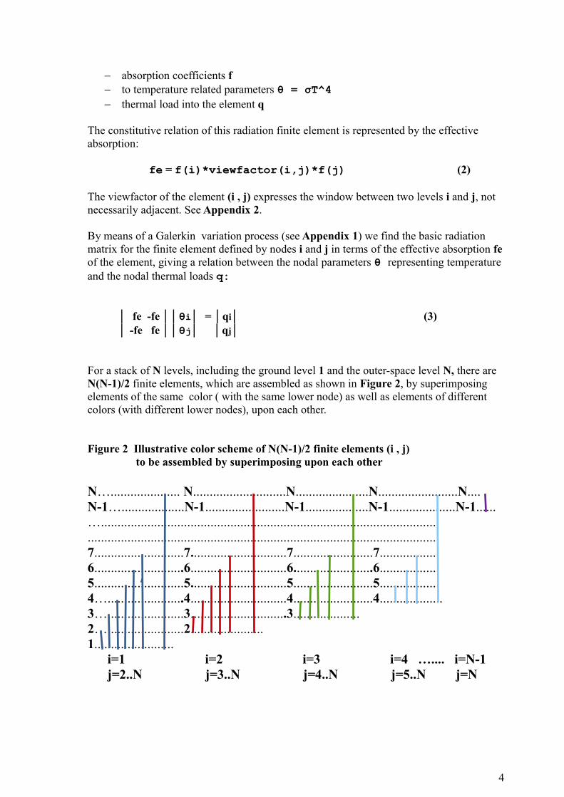
absorption coefficients f to temperature related parameters θ = σT^4 thermal load into the element q
The constitutive relation of this radiation finite element is represented by the effective absorption:
fe = f(i)*viewfactor(i,j)*f(j) (2)
The viewfactor of the element (i , j) expresses the window between two levels i and j, not necessarily adjacent. See Appendix 2.
By means of a Galerkin variation process (see Appendix 1) we find the basic radiation matrix for the finite element defined by nodes i and j in terms of the effective absorption feof the element, giving a relation between the nodal parameters θ representing temperatureand the nodal thermal loads q:
│ fe -fe ││θi│ = │qi│ (3) │ -fe fe ││θj│ │qj│
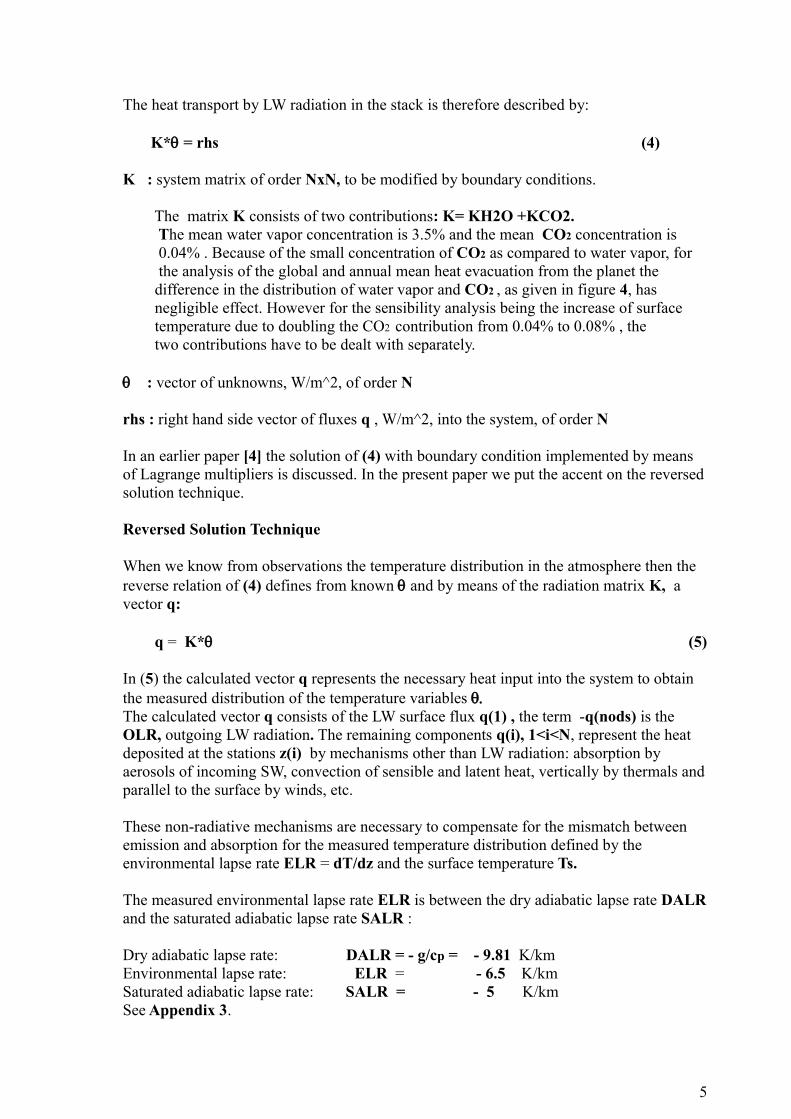
For a stack of N levels, including the ground level 1 and the outer-space level N, there are N(N-1)/2 finite elements, which are assembled as shown in Figure 2, by superimposing elements of the same color ( with the same lower node) as well as elements of different colors (with different lower nodes), upon each other.
Figure 2 Illustrative color scheme of N(N-1)/2 finite elements (i , j) to be assembled by superimposing upon each other
N…..................... N............................N......................N........................N....N-1…...................N-1........................N-1...................N-1....................N-1......…................................................................................................................................................................................................................7...........................7.............................7........................7..................6...........................6.............................6........................6..................5...........................5.............................5........................5..................4….......................4.............................4........................4...................3….......................3.............................3.................... 2….......................2...................... 1........................ i=1 i=2 i=3 i=4 ….... i=N-1 j=2..N j=3..N j=4..N j=5..N j=N
4
The heat transport by LW radiation in the stack is therefore described by:
K* = rhs (4)
K : system matrix of order NxN, to be modified by boundary conditions.
The matrix K consists of two contributions: K= KH2O +KCO2. The mean water vapor concentration is 3.5% and the mean CO2 concentration is 0.04% . Because of the small concentration of CO2 as compared to water vapor, for the analysis of the global and annual mean heat evacuation from the planet the difference in the distribution of water vapor and CO2 , as given in figure 4, has negligible effect. However for the sensibility analysis being the increase of surface temperature due to doubling the CO2 contribution from 0.04% to 0.08% , the two contributions have to be dealt with separately.
: vector of unknowns, W/m^2, of order N
rhs : right hand side vector of fluxes q , W/m^2, into the system, of order N
In an earlier paper [4] the solution of (4) with boundary condition implemented by means of Lagrange multipliers is discussed. In the present paper we put the accent on the reversedsolution technique.
Reversed Solution Technique
When we know from observations the temperature distribution in the atmosphere then the reverse relation of (4) defines from known and by means of the radiation matrix K, a vector q:
q = K* (5)
In (5) the calculated vector q represents the necessary heat input into the system to obtain the measured distribution of the temperature variables The calculated vector q consists of the LW surface flux q(1) , the term -q(nods) is the OLR, outgoing LW radiation. The remaining components q(i), 1<i<N, represent the heat deposited at the stations z(i) by mechanisms other than LW radiation: absorption by aerosols of incoming SW, convection of sensible and latent heat, vertically by thermals andparallel to the surface by winds, etc.
These non-radiative mechanisms are necessary to compensate for the mismatch between emission and absorption for the measured temperature distribution defined by the environmental lapse rate ELR = dT/dz and the surface temperature Ts.
The measured environmental lapse rate ELR is between the dry adiabatic lapse rate DALRand the saturated adiabatic lapse rate SALR :
Dry adiabatic lapse rate: DALR = - g/cp = - 9.81 K/kmEnvironmental lapse rate: ELR = - 6.5 K/kmSaturated adiabatic lapse rate: SALR = - 5 K/kmSee Appendix 3.
5

We can write the components of the vector of temperatures T and of the corresponding vector of variables as function of ELR and z :
Ti = Ts + ELR*zi → i = Ti^4 (6)
The vector q in (5) represents now the necessary heat input at various height in the atmo-sphere to obtain a vector corresponding to a temperature distribution (6) according to the lapse rate ELR. We see that without a model for the various other mechanisms, the deposit of heat by such other mechanisms can be defined, not in detail of each mechanism but the detailed distribution in z-direction of the sum of all.
In view of the proverb “a picture tells more than thousand words ”, we give an example ofthe plots in the next sections where we will deal with the analysis of the atmosphere of the planet.
In Figure 3 are plotted various heat fluxes and/or LW radiation as function of the parameter ftot which is the sum of the absorption coefficient of the grids.A typical value of the number of layers is 50.
For a qtoa = 240 the value ftot= 0.86 is typical. For ftot =0 : OLR= qsurfLW=qwindow = ε1*σ*Ts^4 For increasing ftot, qsurfLW decreases: there is no back-radiation.
Figure 3 Results of equation q = K*
Where:OLR: outgoing LW radiation = - q(nods)qsurfLW: LWsurface flux = q(1)OLR - qsurfLW: mechanisms other than LW radiation = -q(nods)-q(1)qwindow: LW through atmospheric window = (1-ftot) *ε(1)*(1)qLW-in = qsurfLW – qwindow: LW flux into atmosphereqtoa: outgoing LW flux at top of atmosphere, taken as 240 from IPCC.ftot: sum(f)
6
Note the low value of the LW radiation into the atmosphere, qLW-in.Note also the difference between the red and green curve : mechanisms other than LW radiation. These mechanisms are predominant.
Input parameters
Geometry
The results as depicted in figure 3 are obtained from a FEM model with a height = 10 km and number of nodes N=50.
The number of finite elements is N*(N-1)/2= 1225.
Such a high number allows to have a fine mesh near the surface where things happen. A fine mesh is needed there to be able to follow the strong variation of absorption near the surface.
The thickness of the layers dz(i) is defined by a geometrical series with ratio r=1.3 and with sum(dz) equal to height.
The first layer near the surface has a thickness of 6 mm, the upper layer has a thickness of 2.3 km.
Distribution of absorption coefficients
The IR-active gases are those with three or more atoms per molecule: water vapor H20, carbon dioxide CO2, ozone O3, methane CH4.
Water vapor is the predominant IR-active gas: a concentration of 3.5% as the annual and global average. The concentration of CO2 is 0.04% , being about 1% of that of water vapor. The absorption by water vapor molecules is 10 times bigger, and as a consequence the contribution to absorption of CO2 is only 0.1 % of the total one defined by water vapor.However, in the sensitivity analysis two contributions of CO2 are analyzed:0.1 % and 1% of the total contribution of water vapor.
The distribution of the absorption of the water vapor over the various levels with thickness dz(i) is introduced by a function:
fdH2O(i) = α*dz(i)*exp(-m*z(i)/(height/2)) (7)
where m is an input parameter. The constant α is such that the function is normalized: sum(fdH2O)=1.
The distributions fdH2O (7) and fdCO2 (8) are depicted in Figure 4.
7
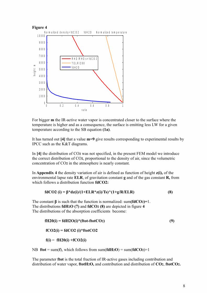
Figure 4
0 0 . 2 0 . 4 0 . 6 0 . 8 10
1 0 0 0
2 0 0 0
3 0 0 0
4 0 0 0
5 0 0 0
6 0 0 0
7 0 0 0
8 0 0 0
9 0 0 0
1 0 0 0 0
r a t i o
heig
ht m
N o r m a l i z e d d e n s i t y = f d C O 2 f d H 2 O N o r m a l i z e d t e m p e r a t u r e
R H O / R H O s = f d C O 2T E L R / 2 8 8f d H 2 O
For bigger m the IR-active water vapor is concentrated closer to the surface where the temperature is higher and as a consequence, the surface is emitting less LW for a given temperature according to the SB equation (1a).
It has turned out [4] that a value m=9 give results corresponding to experimental results by IPCC such as the K&T diagrams.
In [4] the distribution of CO2 was not specified, in the present FEM model we introduce the correct distribution of CO2, proportional to the density of air, since the volumetric concentration of CO2 in the atmosphere is nearly constant.
In Appendix 4 the density variation of air is defined as function of height z(i), of the environmental lapse rate ELR, of gravitation constant g and of the gas constant R, from which follows a distribution function fdCO2:
fdCO2 (i) = β*dz(i)/(1+ELR*z(i)/Ts)^(1+g/R/ELR) (8)
The constant β is such that the function is normalized: sum(fdCO2)=1.The distributions fdH2O (7) and fdCO2 (8) are depicted in figure 4The distributions of the absorption coefficients become:
fH20(i) = fdH2O(i)*(ftot-ftotCO2) (9)
fCO2(i) = fdCO2 (i)*ftotCO2
f(i) = fH20(i) +fCO2(i)
NB ftot = sum(f), which follows from sum(fdH2O) = sum(fdCO2)=1
The parameter ftot is the total fraction of IR-active gases including contribution and distribution of water vapor, ftotH2O, and contribution and distribution of CO2, ftotCO2.
8
The absorption coefficients f(i) as defined in (9) are used in the constitutive relation (2) for the effective absorption fe of the various finite elements.
Application to the real atmosphere.
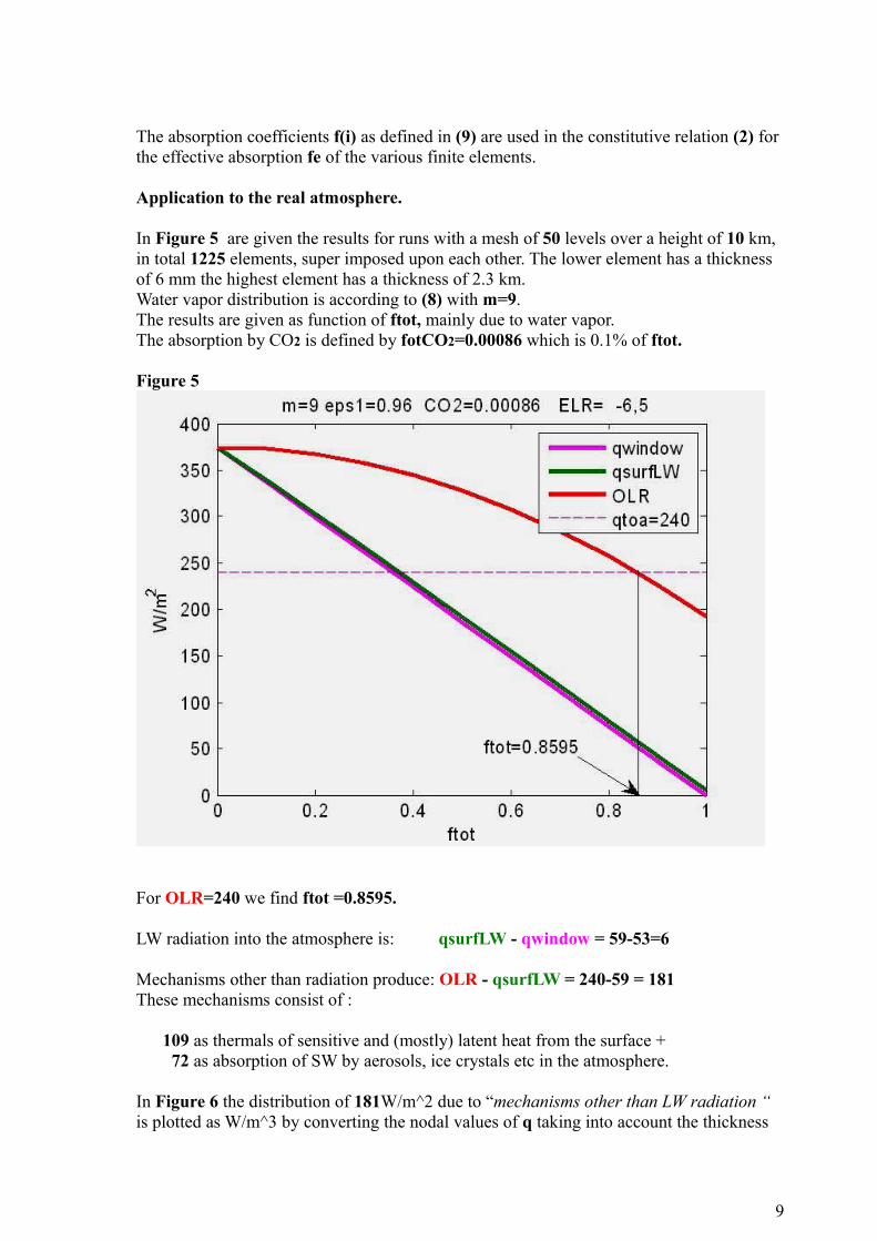
In Figure 5 are given the results for runs with a mesh of 50 levels over a height of 10 km, in total 1225 elements, super imposed upon each other. The lower element has a thickness of 6 mm the highest element has a thickness of 2.3 km. Water vapor distribution is according to (8) with m=9.The results are given as function of ftot, mainly due to water vapor. The absorption by CO2 is defined by fotCO2=0.00086 which is 0.1% of ftot.
Figure 5
For OLR=240 we find ftot =0.8595.
LW radiation into the atmosphere is: qsurfLW - qwindow = 59-53=6
Mechanisms other than radiation produce: OLR - qsurfLW = 240-59 = 181These mechanisms consist of :
109 as thermals of sensitive and (mostly) latent heat from the surface + 72 as absorption of SW by aerosols, ice crystals etc in the atmosphere.
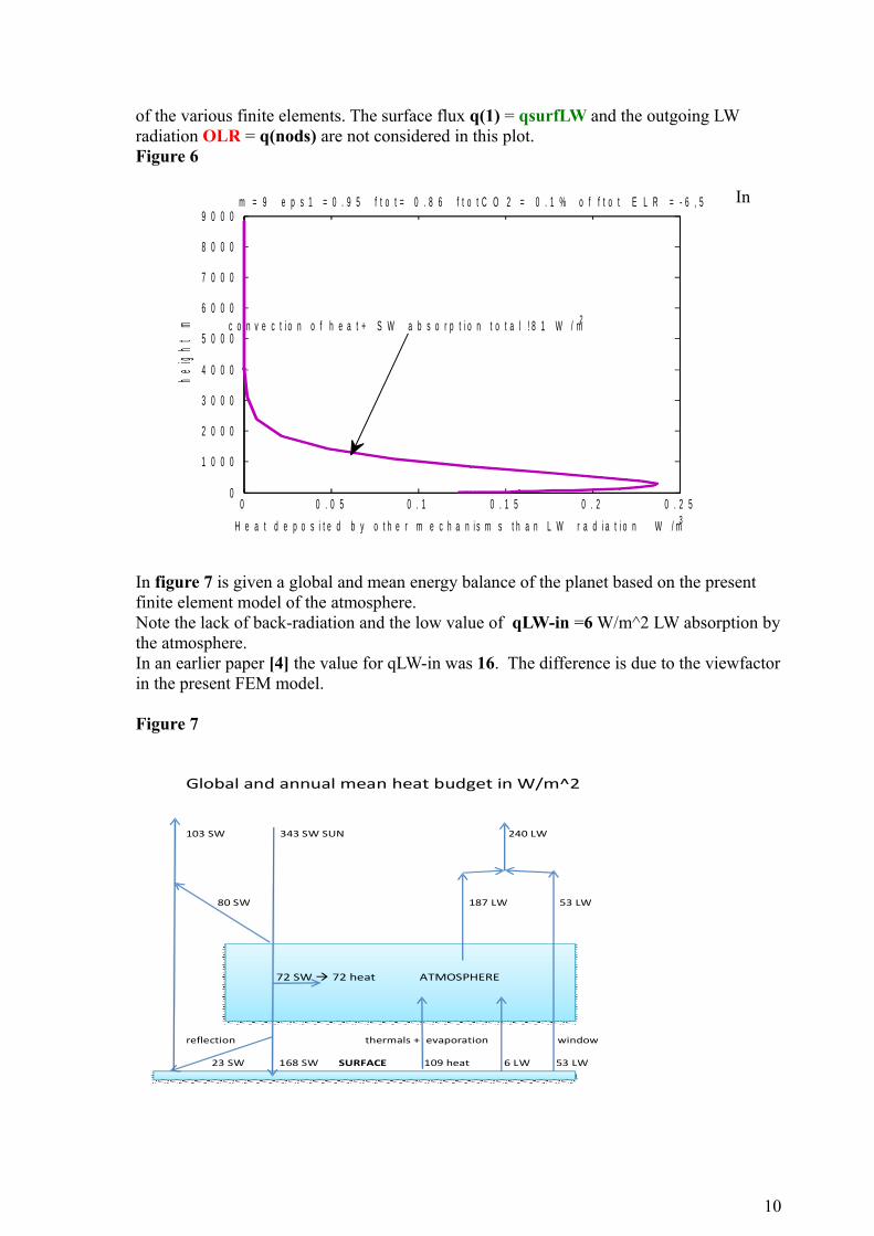
In Figure 6 the distribution of 181W/m^2 due to “mechanisms other than LW radiation “ is plotted as W/m^3 by converting the nodal values of q taking into account the thickness
9
0 0 . 0 5 0 . 1 0 . 1 5 0 . 2 0 . 2 50
1 0 0 0
2 0 0 0
3 0 0 0
4 0 0 0
5 0 0 0
6 0 0 0
7 0 0 0
8 0 0 0
9 0 0 0m = 9 e p s 1 = 0 . 9 5 f t o t = 0 . 8 6 f t o t C O 2 = 0 . 1 % o f f t o t E L R = - 6 , 5
H e a t d e p o s i t e d b y o t h e r m e c h a n i s m s t h a n L W r a d i a t i o n W / m3
heig
ht m c o n v e c t i o n o f h e a t + S W a b s o r p t i o n t o t a l ! 8 1 W / m2
of the various finite elements. The surface flux q(1) = qsurfLW and the outgoing LW radiation OLR = q(nods) are not considered in this plot.Figure 6
In
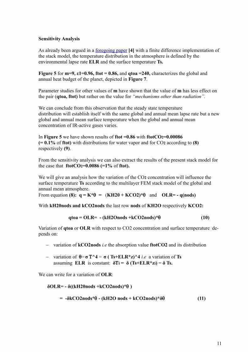
In figure 7 is given a global and mean energy balance of the planet based on the present finite element model of the atmosphere.Note the lack of back-radiation and the low value of qLW-in =6 W/m^2 LW absorption bythe atmosphere. In an earlier paper [4] the value for qLW-in was 16. The difference is due to the viewfactorin the present FEM model.
Figure 7
Global and annual mean heat budget in W/m^2
103 SW 343 SW SUN 240 LW
80 SW 187 LW 53 LW
ATMOSPHERE
thermals
reflection thermals + evaporation window
23 SW 168 SW SURFACE 109 heat 6 LW 53 LW
72 SW 72 heat ATMOSPHERE
10
Sensitivity Analysis
As already been argued in a foregoing paper [4] with a finite difference implementation of the stack model, the temperature distribution in the atmosphere is defined by the environmental lapse rate ELR and the surface temperature Ts.
Figure 5 for m=9, ε1=0.96, ftot = 0.86, and qtoa =240, characterizes the global and annual heat budget of the planet, depicted in Figure 7.
Parameter studies for other values of m have shown that the value of m has less effect on the pair (qtoa, ftot) but rather on the value for “mechanisms other than radiation”.
We can conclude from this observation that the steady state temperature distribution will establish itself with the same global and annual mean lapse rate but a new global and annual mean surface temperature when the global and annual mean concentration of IR-active gases varies.
In Figure 5 we have shown results of ftot =0.86 with ftotCO2=0.00086 (= 0.1% of ftot) with distributions for water vapor and for CO2 according to (8) respectively (9).
From the sensitivity analysis we can also extract the results of the present stack model for the case that ftotCO2=0.0086 (=1% of ftot).
We will give an analysis how the variation of the CO2 concentration will influence the surface temperature Ts according to the multilayer FEM stack model of the global and annual mean atmosphere.From equation (8): q = K* = (KH20 + KCO2)* and OLR= - q(nods)
With kH20nods and kCO2nods the last row nods of KH2O respectively KCO2:
qtoa = OLR= - (kH2Onods +kCO2nods)* (10)
Variation of qtoa or OLR with respect to CO2 concentration and surface temperature de-pends on:
variation of kCO2nods i.e the absorption value ftotCO2 and its distribution
variation of =σ ^4 = σ ( Ts+ELR*z)^4 i.e a variation of Tsassuming ELR is constant: δi = δ (Ts+ELR*zi) = δ Ts.
We can write for a variation of OLR:
δOLR= - δ((kH20nods +kCO2nods)* )
= -δkCO2nods* - (kH2O nods + kCO2nods)*δ (11)
11
The sensibility of the surface temperature for doubling CO2 concentration is defined by imposing δOLR = 0 , assuming sun intensity and albedo do not vary for changing the CO2 concentration from 0.04% to 0,08%. We can write:
B ∆Ts + A ∆ftotCO2 = 0 (12)
The two parameters B and A follow from (11).
i = σ i^4 = (Ts+ELR*zi)^4 δi = (4 σ i^3) δi = (4 σ i^3) δTs (13)
The parameter B becomes:
B = (kH2Onods + kCO2nods)*(4 σ .^3) (14)
For Ts=288, ELR =-6.5 and ftot =0.86 the value becomes:B = 3.38.
The value for A depends only on the CO2 concentration:
A = ∆(kCO2nods* )/ ∆ftotCO2 (15)
(-Prevost + kco2nods* )/∆ftotCO2
The term Prevost is the OLR for ftotCO2=0: Prevost = εσTs0^4 = 374.48
For a value fotCO2=0.00086, OLR is calculated as: kCO2nods* =374.38
The value A becomes: (-374.48 +374.38)/0.00086 = -112.14
The constants A and B have been calculated for ftot=0.86 and ELR= -6.5 and Ts=288 K:
A/B = - 33.216 → ∆Ts = -A/B*∆ftotCO2 = 33.216*∆ftotCO2
For 0.1% contribution of CO2 or ∆ftotCO2= 0.00086 : ∆Ts = 33.216*∆ftotCO2 = 0.03 °C (16)
For 1% contribution of CO2 or ∆ftotCO2 = 0.0086 : ∆Ts = 33.216*∆ftotCO2 = 0.3 °C
12
Conclusions
The finite element model confirms the earlier conclusions of the finite difference model [4].
Once more it is shown that back-radiation does not exist nor the huge atmospheric absorption heralded by IPCC.
The sensitivity study for the surface temperature shows an increase of 0.03°C for a doubling of the CO2 concentration from 0.04% to 0.08%.
Acknowledgments
The author wants to thank in particular Claes Johnson who inspired him to write this paper.The author interpreted his ideas by writing Stefan-Boltzmann always for a pair of surfaces:it opens the concept of standing waves.
The efficient help of Hans Schreuder to edit and to host my papers on his site and give them a broader distribution is appreciated as well as the suggestions by the peer reviewers which Hans has called upon.
Thanks also to readers of previous versions of this paper for their suggestions how to ameliorate its message.
Thanks also to John O'Sullivan at Principia Scientific International for the publication of this paper.
REFERENCES:
[1] http://slayingtheskydragon.com/
[2] http://claesjohnson.blogspot.fr/
[3] http://principia-scientific.org/publications/History-of-Radiation. pdf
[4] http://www.tech-know-group.com/papers/IR-absorption_updated.pdf
13
Appendix 1
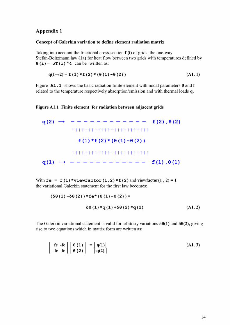
Concept of Galerkin variation to define element radiation matrix
Taking into account the fractional cross-section f (i) of grids, the one-wayStefan-Boltzmann law (1a) for heat flow between two grids with temperatures defined by θ(i)= σT(i)^4 can be written as:
q(1→2) = f(1)*f(2)*(θ(1)-θ(2)) (A1. 1)
Figure A1.1 shows the basic radiation finite element with nodal parameters θ and f related to the temperature respectively absorption/emission and with thermal loads q.
Figure A1.1 Finite element for radiation between adjacent grids
q(2) → — — — — — — — — — — — — f(2),θ(2) ↑↑↑↑↑↑↑↑↑↑↑↑↑↑↑↑↑↑↑↑↑↑↑↑ f(1)*f(2)*(θ(1)-θ(2))
↑↑↑↑↑↑↑↑↑↑↑↑↑↑↑↑↑↑↑↑↑↑↑↑
q(1) → — — — — — — — — — — — — f(1),θ(1)
With fe = f(1)*viewfactor(1,2)*f(2)and viewfactor(1 , 2) = 1 the variational Galerkin statement for the first law becomes:
(δθ(1)-δθ(2))*fe*(θ(1)-θ(2))=
δθ(1)*q(1)+δθ(2)*q(2) (A1. 2)
The Galerkin variational statement is valid for arbitrary variations δθ(1) and δθ(2), giving rise to two equations which in matrix form are written as:
│ fe -fe ││θ(1)│ = │q(1)│ (A1. 3) │ -fe fe ││θ(2)│ │q(2) │
14

Appendix 2
Viewfactor in an element with intermediate grids
In case that in an element, with end faces i and j, intermediate grids are present the exchange of heat by radiation is hindered by viewfactor(i , j). In case of one single intermediate grid: j=i+2:
f (i+2) — — — — — —
f(i+1) — — — — — — viewfactor(i,i+2)=1-f(i+1)
f (i) — — — — — —
The viewfactor reflects the fact that radiation from level i to level i+2 is hindered by the grid i+1.
In case more grids k are present between level i and level j, with i<k<j, the viewfactor of element (i, j) becomes:
k = j-1
viewfactor(i , j) = 1 – Σ f(k) (A2.1) k = i+1
The so-called atmospheric windows from node i to outer space node N is a special case of the more general view-factors:
window(i) = viewfactor(i , N) (A2.2)
The effective absorption/emission of element (i , j) becomes:
fe(i , j) = f(i)*viewfactor(i , j)*f(j) (A2.3)
Appendix 3
Lapse rates
The dry adiabatic lapse rate DALR is the thermal gradient dT/dz of dry air due the adiabatic compression/expansion of air.It follows from the ideal gas law, being an equation of state for the 3 properties: pressure p [N/m^2], density ρ [kg/m^3], temperature T [K]and the gravitation law of Newton.
15
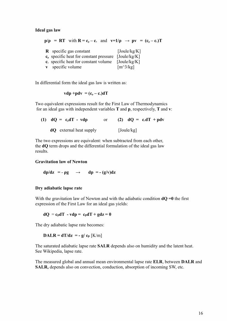
Ideal gas law
p/ρ = RT with R = cp – cv and v=1/ρ → pv = (cp – cv)T
R specific gas constant [Joule/kg/K] cp specific heat for constant pressure [Joule/kg/K] cv specific heat for constant volume [Joule/kg/K] v specific volume [m^3/kg]
In differential form the ideal gas law is written as: vdp +pdv = (cp – cv)dT
Two equivalent expressions result for the First Law of Thermodynamics for an ideal gas with independent variables T and p, respectively, T and v: (1) dQ = cpdT - vdp or (2) dQ = cvdT + pdv
dQ external heat supply [Joule/kg]
The two expressions are equivalent: when subtracted from each other, the dQ term drops and the differential formulation of the ideal gas lawresults.
Gravitation law of Newton
dp/dz = - ρg → dp = - (g/v)dz
Dry adiabatic lapse rate With the gravitation law of Newton and with the adiabatic condition dQ =0 the first expression of the First Law for an ideal gas yields:
dQ = cpdT - vdp = cpdT + gdz = 0
The dry adiabatic lapse rate becomes:
DALR = dT/dz = - g/ cp [K/m]
The saturated adiabatic lapse rate SALR depends also on humidity and the latent heat. See Wikipedia, lapse rate.
The measured global and annual mean environmental lapse rate ELR, between DALR andSALR, depends also on convection, conduction, absorption of incoming SW, etc.
16
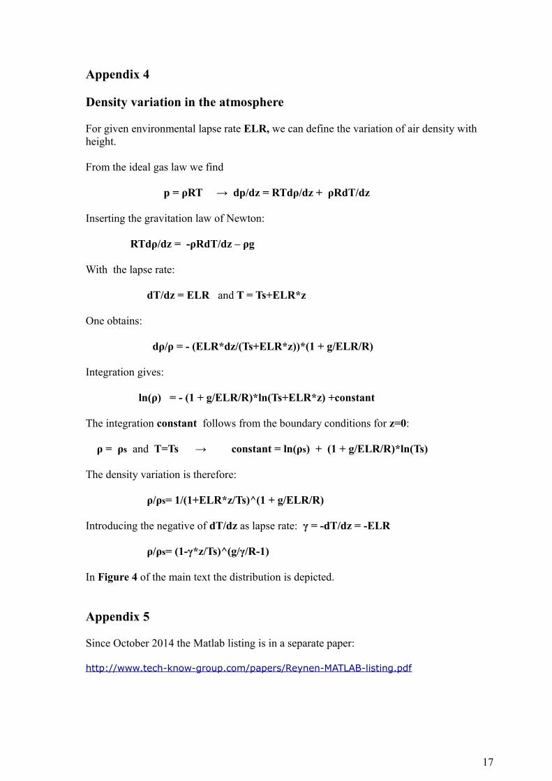
Appendix 4
Density variation in the atmosphere
For given environmental lapse rate ELR, we can define the variation of air density with height.
From the ideal gas law we find
p = ρRT → dp/dz = RTdρ/dz + ρRdT/dz
Inserting the gravitation law of Newton:
RTdρ/dz = -ρRdT/dz – ρg
With the lapse rate:
dT/dz = ELR and T = Ts+ELR*z
One obtains: dρ/ρ = - (ELR*dz/(Ts+ELR*z))*(1 + g/ELR/R)
Integration gives:
ln(ρ) = - (1 + g/ELR/R)*ln(Ts+ELR*z) +constant
The integration constant follows from the boundary conditions for z=0:
ρ = ρs and T=Ts → constant = ln(ρs) + (1 + g/ELR/R)*ln(Ts)
The density variation is therefore:
ρ/ρs= 1/(1+ELR*z/Ts)^(1 + g/ELR/R)
Introducing the negative of dT/dz as lapse rate: γ = -dT/dz = -ELR
ρ/ρs= (1-γ*z/Ts)^(g/γ/R-1)
In Figure 4 of the main text the distribution is depicted.
Appendix 5
Since October 2014 the Matlab listing is in a separate paper:
http://www.tech-know-group.com/papers/Reynen-MATLAB-listing.pdf
17

18