FINITE ELEMENT PREDICTIONS OF PLASTICITY–INDUCED FATIGUE ...
119
FINITE ELEMENT PREDICTIONS OF PLASTICITY–INDUCED FATIGUE CRACK CLOSURE IN THREE-DIMENSIONAL CRACKED GEOMETRIES By Jeffrey David Skinner, Jr. A Thesis Submitted to the Faculty of Mississippi State University in Partial Fulfillment of the Requirements for the Degree of Master of Science in Mechanical Engineering in the Department of Mechanical Engineering Mississippi State, Mississippi August 2001
Transcript of FINITE ELEMENT PREDICTIONS OF PLASTICITY–INDUCED FATIGUE ...

FINITE ELEMENT PREDICTIONS OF PLASTICITY–INDUCED FATIGUE CRACK
CLOSURE IN THREE-DIMENSIONAL CRACKED GEOMETRIES
By
Jeffrey David Skinner, Jr.
A Thesis Submitted to the Faculty of Mississippi State University
in Partial Fulfillment of the Requirements for the Degree of Master of Science
in Mechanical Engineering in the Department of Mechanical Engineering
Mississippi State, Mississippi
August 2001
Name: Jeffrey David Skinner, Jr.
Date of Degree: August 4, 2001
Institution: Mississippi State University
Major Field: Mechanical Engineering
Major Advisor: Dr. Steven R. Daniewicz
Title of Study: FINITE ELEMENT PREDICTIONS OF PLASTICITY-INDUCED CRACK CLOSURE IN THREE-DIMENSIONAL CRACKED GEOMETRIES
Pages in Study: 109 Candidate for Degree of Master of Science Elastic-plastic finite element analyses were performed to predict the crack
opening level profiles in semi-elliptical surface cracks. A script was written to use the
commercial finite element code ANSYS to predict opening levels in cracked geometries.
The functionality of the scripts was verified by comparing predicted opening levels in
two and three-dimensional center-cracked geometries to experimental results. In
addition, a parameter study was performed in which various aspects of the modeling
routine were modified. This included a mesh refinement study as well as a study into the
effect of a strain hardening material. The main focus of the current research, however, is
to compare finite element predicted opening levels with published opening levels
determined experimentally. The finite element predicted opening levels were in all cases
significantly lower than those reported experimentally, however, similar trends in both
crack opening level profile along the crack front, and opening level variations with crack
growth were shown.

FINITE ELEMENT PREDICTIONS OF PLASTICITY–INDUCED FATIGUE CRACK
CLOSURE IN THREE-DIMENSIONAL CRACKED GEOMETRIES
By
Jeffrey David Skinner, Jr.
Approved: _________________________________ _________________________________ Steven R. Daniewicz E. William Jones Associate Professor of Mechanical Professor of Mechanical Engineering Engineering (Director of Thesis) (Committee Member) _________________________________ _________________________________ James C. Newman, III Rogelio Luck Assistant Professor of Aerospace Associate Professor of Mechanical Engineering and Engineering Mechanics Engineering (Committee Member) (Committee Member) Graduate Coordinator of the Department of Mechanical Engineering _________________________________ A. Wayne Bennett Dean of the College of Engineering

-ii-
ACKNOWLEDGMENTS
I would like to express sincere gratitude to the many people without whose
selfless assistance this thesis could not have materialized. First of all, sincere thanks are
due to Dr. Steven R. Daniewicz, my major advisor, for his magnanimity in expending
time and effort to guide and assist me throughout this research and for opening the door
on many professional opportunities along the way. Second, I would like to thank Dr.
James C. Newman, Jr. of NASA Langley Research Center for allowing me the
opportunity to spend two summers at Langley under his mentorship, and for providing
me with a finite element code for direct comparison with my results. Also, expressed
appreciation is due to the other members of my thesis committee, namely, Dr. E. William
Jones, Dr. James C. Newman, III, and Dr. Rogelio Luck, for the invaluable aid and
direction provided by them. Finally, I would like to thank Dr. Robert H. Dodds, Jr. of the
University of Illinois at Urbana-Champaign for making available the computer program
for the generation of the surface crack meshes used in this study.

iii
TABLE OF CONTENTS
Page
ACKNOWLEDGEMENTS ...................................................................................... ii
LIST OF TABLES .................................................................................................... vi
LIST OF FIGURES................................................................................................... vii
CHAPTER
I. INTRODUCTION................................................................................... 1
1-1 Fatigue Crack Propagation............................................................... 2 1-2 Fatigue Crack Closure...................................................................... 4 1-3 Variable Amplitude Loading ........................................................... 6 1-4 Crack Nomenclature ........................................................................ 7 II. LITERATURE REVIEW........................................................................ 9 2-1 Two-Dimensional Modeling Issues ................................................. 10 2-1-1 Element Type.......................................................................... 10 2-1-2 Appropriate Mesh Size ........................................................... 10 2-1-3 Crack Opening Level Determination...................................... 11 2-1-4 Crack Opening Level Stabilization......................................... 11 2-1-5 Crack Advance Scheme.......................................................... 11 2-1-6 Constitutive Model ................................................................. 12 2-2 Applications of Crack Closure Models............................................ 12 III. FINITE ELEMENT PROCEDURE........................................................ 14 3-1 Basic Finite Element Issues ............................................................. 15 3-1-1 Element Type.......................................................................... 15 3-1-2 Plasticity Model...................................................................... 16 3-1-3 Equation Solver and Non-Linear Solution Control ................ 16 3-1-4 Model Symmetry .................................................................... 17 3-1-5 Mesh Generation..................................................................... 18

iv
CHAPTER Page 3-1-6 Mesh Refinement.................................................................... 19 3-2 Crack Closure Related Issues........................................................... 21 3-2-1 Crack Advance ....................................................................... 21 3-2-2 Crack Surface Contact ............................................................ 22 3-3 Closure Model Overview................................................................. 24 IV. PRELIMINARY SCRIPT VERIFICATION.......................................... 26 4-1 Two-Dimensional Verification ........................................................ 26 4-2 Three-Dimensional Verification ...................................................... 29 4-2-1 Results of Through-Crack Analysis ....................................... 30 4-2-2 Direct Comparison with Zip3d ............................................... 31 V. MODELING PARAMTER EFFECTS ................................................... 33 5-1 ANSYS Specific Paramters ............................................................. 34 5-1-1 Equation Solver Tolerance ..................................................... 34 5-1-2 Non-Linear Solution Control.................................................. 35 5-2 General Checks ................................................................................ 36 5-2-1 Mesh Refinement Study ......................................................... 36 5-2-2 Load Increment Effect ............................................................ 37 5-2-3 Remote Boundary Conditions ................................................ 38 5-2-4 Large Deformation Effects ..................................................... 39 5-2-5 Strain Hardening..................................................................... 40 5-3 Summary.......................................................................................... 42 VI. COMPARISON WITH EXPERIMENTAL RESULTS ......................... 43 6-1 Finite Element Model Description................................................... 44 6-2 Analysis Results............................................................................... 45 6-3 Conclustions..................................................................................... 50 VII. SUMMARY AND CONCLUSIONS ..................................................... 52 7-1 Parameter Study............................................................................... 52 7-2 Comparison with Experimental Results........................................... 53 7-3 Recommended Future Work ............................................................ 53 REFERENCES.......................................................................................................... 55
APPENDIX
A.1 ANSYS INPUT FILE APPBCS.MAC..................................................... 58
v
APPENDIX Page
A.2 ANSYS INPUT FILE STRTCYC.MAC................................................... 62
A.3 ANSYS INPUT FILE FIRSTLOAD.MAC .............................................. 64 A.4 ANSYS INPUT FILE ADVANCECRACK.MAC .................................... 66 A.5 ANSYS INPUT FILE UNLOADCRACK.MAC ...................................... 69 A.6 ANSYS INPUT FILE LOADCRACK.MAC............................................ 73 A.7 ANSYS INPUT FILE APPLOAD.MAC ................................................. 77 A.8 ANSYS INPUT FILE CLEARRST.MAC ................................................ 79 A.9 ANSYS INPUT FILE SELCTNODES.MAC........................................... 81 B.1 INPUT FILE THROUGHCRACK.DAT .................................................. 83 B.2 INPUT FILE PCA0631.DAT................................................................... 86 C CLOSURE ROUTINE USER’S GUIDE................................................ 89 D FORTRAN PROGRAM ANSMESH54.FOR .......................................... 94 E INPUT FILE MESH3D_SCPCELL.IN .................................................. 104 F FORTRAN PROGRAM CLOSINTERP.F90.......................................... 106

vi
LIST OF TABLES
TABLE Page 6-1 Models Used to Compare with Experimental Data........................... 44

vii
LIST OF FIGURES
FIGURE Page 1-1 Crack Growth Behavior .................................................................... 3 1-2 Crack Closure Mechanisms............................................................... 4 1-3 Schematic of Effective Stress Intensity Factor Range ...................... 6 1-4 Variable Amplitude Loading Effects ................................................ 7 1-5 Crack Regions of Interest.................................................................. 8 3-1 Linear Elements in Two and Three Dimensions............................... 15 3-2 Bi-Linear Plasticity Model ................................................................ 16 3-3 Model Symmetry............................................................................... 18 3-4 Interpolation of Node Opening Load ................................................ 23 3-5 Typical Load Cycle ........................................................................... 24 4-1 Two-Dimensional Finite Element Mesh ........................................... 27 4-2 Two-Dimensional Model Results ..................................................... 28 4-3 Three-Dimensional Center-Cracked Panel........................................ 30 4-4 Stabilized Opening Levels in Three-Dimensional Model................. 31 4-5 Remote Boundary Condition Effects ................................................ 32 5-1 Model Used for Parameter Studies.................................................... 34 5-2 Solver Tolerance Effect..................................................................... 35 5-3 Non-Linear Solution Control ............................................................ 36
viii
FIGURE Page 5-4 Mesh Refinement Study.................................................................... 37 5-5 Load Increment Effect....................................................................... 38 5-6 Effect of Remote Boundary Conditions ............................................ 39 5-7 Large Deformation Effects................................................................ 40 5-8 Strain Hardening Effects ................................................................... 41 6-1 Typical Finite Element Mesh, PCA 06 a/t = 0.55............................. 45 6-2 Crack Opening Level Stabilization ................................................... 46 6-3 PCA 06 Crack Opening Levels ......................................................... 47 6-4 PCA 13 Crack Opening Levels ......................................................... 48 6-5 PCA 15 Crack Opening Levels ......................................................... 48 6-6 Typical Plastic Zone.......................................................................... 49 6-7 Comparison of Stabilized Deep Point Opening Levels..................... 50
1
CHAPTER I
INTRODUCTION
It has been suggested that 50 to 90 percent of all mechanical failures are due to
fatigue, and the majority of these failures are unexpected (Stephens, 2001). Fatigue
causes failure in many common items such as door springs, toothbrushes, and tennis
racquets as well more complex components and structures in automobiles, ships, and
aircraft as well as any other device which undergoes repeated loading. In 1978, a
comprehensive study indicated a cost of $119 billion (in 1982 dollars) or roughly 4
percent of the gross national product due to fracture in the United States (ASTM, 2000).
This study suggested that using proper and current technology in design could
significantly reduce this cost.
There are currently many approaches to fatigue design. Some are simple and
inexpensive; others are extremely complex and expensive. If initially an expensive
complete fatigue design procedure is implemented, this may lead to lower cost in the long
run by reducing failure. Proper characterization of fatigue behavior can lead to the
design of more competitive products. In the aircraft and automotive industries this can
mean lighter structures.

2
Damage tolerant methodology can be used for designing initially flawed
components or determining the remaining life to failure once a flaw is detected. This is
particularly of interest to the aircraft industry, where cracks are commonly detected and
monitored in nearly every structural component of the aircraft.
The current researches focuses on a subset of the current damage tolerant
methodology, fatigue crack closure. This chapter serves to give a brief introduction to
fatigue crack closure and how it is applied to practical design. It should be noted that all
the concepts introduced in this chapter apply to metallic materials.
1-1 Fatigue Crack Propagation
If an engineering structure, which can be any load bearing component of a
complex assembly, is subjected to repeated or cyclic loading, the structure is inherently
accumulating fatigue damage. Eventually, if the cycled loads are large enough, a crack
will form that can be detected and the question becomes how long it will take the crack to
reach a critical length where rapid fracture will take place. These cycles between crack
detection and structural failure are where fatigue crack propagation takes place. Figure 1-
1 shows a schematic of the regions of crack growth.

3
m
IIParis Regime
IIIFracture
IThreshold
∆Kth KcLOG ∆K
LOG
da dN
Figure 1-1 Crack Growth Behavior
This figure shows three distinct regions of crack growth. The abscissa of
this plot is the difference between the stress intensity factor (which is a function of load,
crack length, and geometry) at the maximum load and minimum load on logarithmic
scale. The ordinate is the crack growth per cycle. Region I is the threshold regime where
small changes in load (which directly affects the stress intensity factor) results in little to
no detectable crack growth. Region III is the fracture regime where the maximum stress
intensity factor is approaching the material dependant fracture toughness, where rapid
fracture will take place. Region II is the most significant region, which has become
known as the Paris regime. Crack growth is nearly linear with changes in stress intensity
factor range. The well known Paris equation can be used to model crack propagation in
this region:
(1-1)
( )mKC
dNda ∆=

4
where C and m are material properties. For a given crack length and load level, this
equation can be integrated to determine the number of cycles before the crack length
reaches its critical length.
1-2 Fatigue Crack Closure
In 1970, Wolf Elber quantified and demonstrated the importance of a new fatigue
crack growth phenomena, crack closure (Elber, 1970). Based on experimental results
using thin sheets of an aluminum alloy, Elber argued that a reduction in the crack tip
driving force occurred as a result of residual tensile deformation left in the wake of a
growing crack. The residual tensile deformation caused the crack surfaces to close
prematurely before minimum load was reached. Figure 1-2 shows a schematic
representation of the mechanisms causing fatigue crack closure (Anderson, 1995).
Plasticity-Induced Roughness-Induced
Mode II Displacement
Oxide-Induced
Oxide Debris
Viscous Fluid Induced
Fluid
Transformation-Induced
Transformed Zone
Figure 1-2 Crack Closure Mechanisms

5
Of particular importance to the current research is plasticity-induced crack
closure. It is this type of closure that was first observed by Elber, and is caused by
residual tensile deformations in the wake of a growing crack. The other closure
mechanisms are often assumed to be secondary, however multiple closure mechanisms
can be present at once, increasing the closure level.
Figure 1-3 shows the effect closure has on cyclic loading. It is assumed that no
crack growth takes place during the portion of the load cycle when the crack surfaces are
closed. This is implemented in the crack growth propagation equation by using a
modified Paris equation that uses an effective stress intensity range to determine crack
growth.
(1-2)
(1-3)
Unfortunately, however, determination of the crack opening level is difficult. For
plasticity-induced closure, approximate methods have been developed to calculate
opening levels, but to ensure the accuracy of the results complex elastic-plastic finite
element analyses must be performed.
( )opeff
meff
KKK
KCdNda
−=∆
∆=
max

6
Time
K
Kmax
Kmin
Kop
∆K∆Keff
Figure 1-3 Schematic of Effective Stress Intensity Factor
The current research focuses on using elastic-plastic finite element analysis to
predict plasticity-induced closure in three-dimensional geometries, particularly in a semi-
elliptical flawed geometry. The predicted opening levels are compared with
experimentally obtained levels.
1-3 Variable Amplitude Loading
Plasticity-induced crack closure is of particular interest when variable amplitude
loading is used. Plasticity-induced crack closure under the influence of variable
amplitude loading violates the concept of similitude (Anderson, 1995). Similitude
implies that the crack tip conditions are uniquely defined by a single loading parameter.
This is clearly not the case when variable amplitude loading is used (Figure 1-4). The
crack tip stress state is complicated by the loading history. It is in these types of loading
conditions that plasticity induced crack closure really influences crack growth behavior.

7
TIME
KI
TIME
KI
TIME
KIIncreasing K:
Decreasing K:
Random Loading:
Figure 1-4 Variable Amplitude Loading Effects
1-4 Crack Nomenclature
Throughout this document, references are made to specific regions around the
crack front. Figure 1-4 shows the regions of interest. In speaking of these regions, they
are described with reference to the location of the crack front. For instance, the area to
the right of the crack tip in this figure will be referenced as “ahead of the crack tip”.
Similarly, the region to the left is “behind the crack tip”. Also, throughout this document
are references to the crack tip plastic zones. Normally, the crack tip plastic zone refers to
the crack forward plastic zone. This is the region of yielded material ahead of the crack
tip at maximum load. The reverse plastic zone is the region of material ahead of the

8
crack tip that yields in compression at the minimum load. When referring to plastic zone
sizes in this document, this is the size of the plastic zone on the crack plane. Further, as
the crack progresses through the initial plastic zone, yielded material with residual
stresses is left behind the crack tip, this region is referred to as the plastic wake.
ForwardPlastic Zone
ReversePlastic Zone
CrackPlane
PlasticWake
Figure 1-5 Crack Regions of Interest

9
CHAPTER II
LITERATURE REVIEW
A number of researchers have attempted modeling plasticity-induced crack
closure using the finite element method. A useful historical and critical review of these
analyses has been presented by McClung (McClung, 1999). While some researchers
have attempted three-dimensional models, the majority of the finite element analyses
performed model crack closure in two-dimensional geometries. While simplistic in
nature, the results from the two-dimensional analyses are important because they give
insight into some of the more common modeling issues related to crack closure.
The basic algorithm employed by all the studies investigated is the same. A mesh
is created with a suitably refined region near the crack front. An elastic-plastic material
model is employed so plastic deformations occur in the vicinity of the crack tip. Remote
tractions are then applied to the model and cycled between a maximum nominal stress
Smax and a minimum nominal stress Smin. Sometime during the load cycle, the crack front
nodes are released, advancing the crack one elemental length da, which allows for the
formation of a plastic wake. Stresses and displacements for the crack surface nodes are
monitored to detect contact between crack faces, and thus predict crack closure. This
process is repeated for several load cycles until the crack opening stress values stabilize.

10
2-1 Two Dimensional Modeling Issues
2-1-1 Element Type
Early two-dimensional analyses were performed with constant strain triangle
elements (Newman, 1976). More recently, however, researchers commonly use linear
four noded quadrilateral elements or quadratic eight noded quadrilateral elements. The
choice of element selected is most often driven by computer hardware limitations.
Dougherty et al., however, observed that the quadratic elements produced unacceptable
residual stresses in the crack wake and recommended using linear quadrilateral elements
with an aspect ratio of 2 (Dougherty, 1997).
2-1-2 Appropriate Mesh Size
One of the most important modeling considerations when modeling plasticity-
induced crack closure using the finite element method is the choice of an appropriate
mesh. Usually the appropriateness of the mesh is determined by comparing the elemental
length at the crack tip in the crack growth direction ∆a to the forward plastic zone size rp.
This is appropriate because the element size on the crack plane determines the crack
growth increment and also influences how accurately the crack-tip plasticity is
discretized. Among the first to perform mesh refinement studies on these type models
was Newman, who determined increasingly refined meshes give equivalent results, and
coarser meshes are inadequate at lower applied loads (Newman, 1976). McClung later
interpreted these analyses in terms of a ratio of element size to plastic zone width on the
crack plane (McClung, 1989). It was determined that for R = 0, the ratio ∆a / rp = 0.10,

11
which was later determined to be equivalent to coincide with the reverse plastic zone size
for R =0 (McClung, 1991). The appropriateness of this mesh size was later confirmed by
Dougherty et al. (Dougherty, 1997).
2-1-3 Crack Opening Level Determination
Most researchers used a simple method of determining the crack opening level.
The crack opening level is usually determined by detecting tensile stresses in the
elements behind the crack tip. The load at which the last element behind the crack tip
becomes tensile is the crack opening level. Similarly, the crack closing load is the load at
which the nodes behind the crack tip exhibit negative displacements. It was later
suggested by Wu and Ellyin that the above method is in error, and they instead proposed
that only the reaction force at the crack tip should be monitored (Wu, 1996). When the
crack tip reaction force becomes tensile, the crack is open and similarly the crack is
closed when the reaction force becomes compressive.
2-1-4 Crack Opening Level Stabilization
The number of cycles required for stabilization of crack opening levels is often a
function of the mesh refinement. McClung suggests that the crack must be grown
through its initial forward plastic zone before stabilization is achieved (McClung, 1989).
Park et al. later confirmed this criterion (Park, 1997).
2-1-5 Crack Advance Scheme
One of the most contentious modeling issues in crack closure modeling using
FEA has been the crack advance scheme, particularly when during the load cycle crack

12
advance should take place. Most commonly, crack advance takes place at either
maximum or minimum load. Researchers implementing crack advance at maximum load
do so because crack growth at maximum load is physically more realistic (Newman,
1976). However, advance at maximum load has been observed to cause an artificial
perturbation in the crack tip stress-strain history and also leads to convergence
difficulties, so crack advance at minimum load is a sensible alternative (McClung,
1989a). Some analyses have shown that there is no difference in the results obtained
from the two differing crack advance schemes (McClung 1989a)(Wu, 1996) while others
show significant differences (Park, 1997)(Wu, 1996).
2-1-6 Constitutive Model
Most researchers assume a material that is elastic-perfectly plastic. However,
some research has been performed to determine the effect of material hardening. A
significant change in opening behavior was found when different hardening slopes where
assumed. For low loads (Smax / σ0 < 0.6) a higher hardening modulus resulted in lower
opening levels (McClung, 1989b).
2-2 Applications of Crack Closure Models
The majority of research discussed here concentrated on basic constant amplitude
behavior. The fundamental effects of maximum stress and stress ratio on opening levels
have been characterized (Newman, 1976), and results seem to agree with simple
analytical models (McClung, 1989a). Crack opening levels decrease with increasing
maximum stress and also decrease with decreasing R.
13
Some researchers have investigated the effects of different load histories on crack
closure. Newman showed the effects of high-low and low-high block loading on crack
closure behavior (Newman, 1976). Dougherty investigated the effects of single spike
overloads on crack closure (Dougherty, 1997). Also, load-shedding effects on closure
has been modeled successfully using finite element models (McClung, 1991) (Daniewicz,
2000).
Because of computer hardware limitations, few researchers have attempted to
model closure in three-dimensional models. The majority of the three dimensional
modeling has been used on center-cracked geometries, where the crack opening profile
along the crack front as it varies from plane strain to plane stress is investigated
(Chermahini, 1989a)(Chermahini, 1989b)(Riddell, 1999)(Daniewicz, 2000)(Seshadri,
1995). Also, some attempts have been made at modeling crack closure in semi-elliptical
flawed geometries (Seshadri, 1995)(Chermahini, 1993)(Zhang, 1998). All of these
attempts, however, suffer from possible mesh inadequacies.
14
CHAPTER III
FINITE ELEMENT PROCEDURE
A routine was written in ANSYS Parametric Design Language (APDL) to model
plasticity-induced fatigue crack closure in arbitrary geometries. It is the purpose of this
chapter to give an explanation to all the steps involved in the routine as well as give a
brief overview of the entire routine. A command listing for all the routines involved is
included in Appendix A. Sample input files for a three-dimensional center cracked
model and an elliptical surface crack model are included in Appendix B. Also, a concise
user’s guide for the scripts can be found in Appendix C.
The basic algorithm for modeling plasticity induced fatigue crack closure is
elementary. A mesh is created that is suitably refined near the crack front. Remote loads
are applied to the model and are cycled between a maximum and a minimum load.
Sometime during each of these load cycles, the crack front nodes are released, advancing
the crack one elemental length. After several crack growth cycles are completed, a
plastic wake is formed resulting in crack closure.
The following section describes some of the basic finite element issues associated
with this routine. This is followed by a discussion of the issues relating specifically to
modeling plasticity-induced fatigue crack closure. The chapter is then concluded with a
brief overview of the entire modeling process.
15
3-1 Basic Finite Element Issues
3-1-1 Element Type
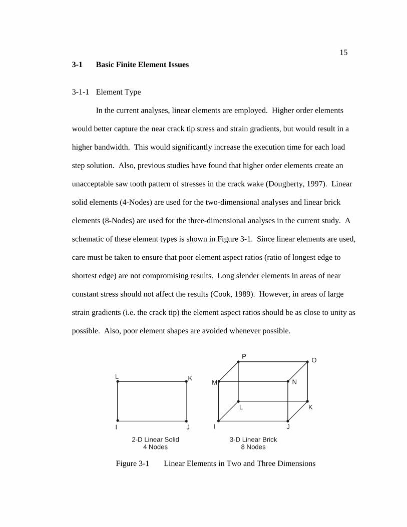
In the current analyses, linear elements are employed. Higher order elements
would better capture the near crack tip stress and strain gradients, but would result in a
higher bandwidth. This would significantly increase the execution time for each load
step solution. Also, previous studies have found that higher order elements create an
unacceptable saw tooth pattern of stresses in the crack wake (Dougherty, 1997). Linear
solid elements (4-Nodes) are used for the two-dimensional analyses and linear brick
elements (8-Nodes) are used for the three-dimensional analyses in the current study. A
schematic of these element types is shown in Figure 3-1. Since linear elements are used,
care must be taken to ensure that poor element aspect ratios (ratio of longest edge to
shortest edge) are not compromising results. Long slender elements in areas of near
constant stress should not affect the results (Cook, 1989). However, in areas of large
strain gradients (i.e. the crack tip) the element aspect ratios should be as close to unity as
possible. Also, poor element shapes are avoided whenever possible.
I J
KL
M N
OP
I J
KL
2-D Linear Solid4 Nodes
3-D Linear Brick8 Nodes
Figure 3-1 Linear Elements in Two and Three Dimensions
16
3-1-2 Plasticity Model
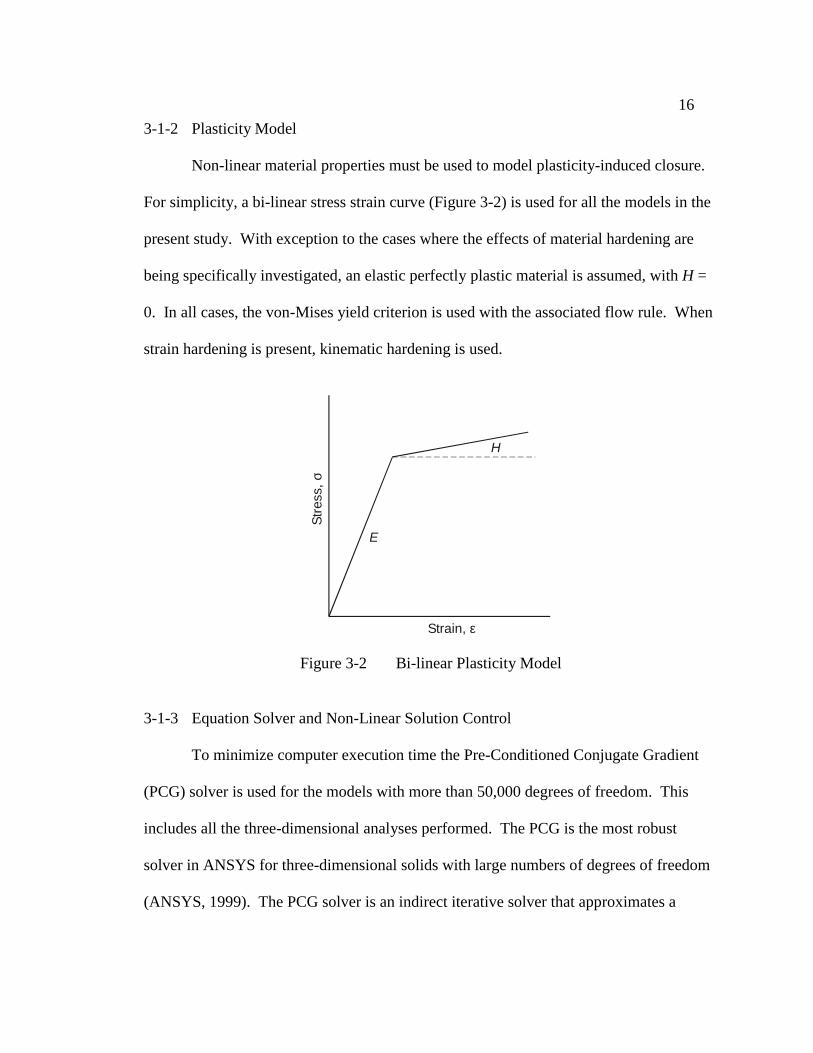
Non-linear material properties must be used to model plasticity-induced closure.
For simplicity, a bi-linear stress strain curve (Figure 3-2) is used for all the models in the
present study. With exception to the cases where the effects of material hardening are
being specifically investigated, an elastic perfectly plastic material is assumed, with H =
0. In all cases, the von-Mises yield criterion is used with the associated flow rule. When
strain hardening is present, kinematic hardening is used.
H
E
Strain, ε
Stre
ss, σ
Figure 3-2 Bi-linear Plasticity Model
3-1-3 Equation Solver and Non-Linear Solution Control
To minimize computer execution time the Pre-Conditioned Conjugate Gradient
(PCG) solver is used for the models with more than 50,000 degrees of freedom. This
includes all the three-dimensional analyses performed. The PCG is the most robust
solver in ANSYS for three-dimensional solids with large numbers of degrees of freedom
(ANSYS, 1999). The PCG solver is an indirect iterative solver that approximates a

17
solution to within a specified convergence tolerance. The effect of varying this tolerance
is investigated in a subsequent chapter. For the smaller two-dimensional models the
ANSYS sparse solver is used.
Because of the non-linear nature of plasticity, non-linear solution control with
automatic time stepping is used to control convergence. The full Newton-Rhapson
method with adaptive descent is used to solve the non-linear equations. Automatic time
stepping is used to increase the number substeps when convergence is not occurring
within a given number of equilibrium iterations, or when the maximum equivalent plastic
strain in the model exceeds 15%. This breaks each of the load steps into smaller steps to
ease convergence. When convergence occurs rapidly the number of substeps is
decreased to speed run-time. The non-linear solution control functions are implicit to
ANSYS, and default parameters are used.
3-1-4 Model Symmetry
All of the geometries investigated in the current study contain at least two planes
of symmetry. First, there is a plane of symmetry that contains the crack plane. This is
important because it is in this plane that crack surface closure is monitored. Also, the
center cracked tension (CCT) geometries have planes of symmetry halfway through the
thickness and halfway through the width. The surface crack geometries also exhibit a
plane of symmetry halfway through the width. The planes of symmetry for these
geometries are shown in Figure 3-3.

18
Center Crack3-Symmetry Planes
Surface Crack2-Symmetry Planes
Figure 3-3 Model Symmetry
3-1-5 Mesh Generation
Mesh generation for the two-dimensional models and the three-dimensional
center-crack models was performed using the ANSYS preprocessor. Because of the
complexities in building a mesh for a semi-elliptical surface crack, an external
FORTRAN program was used. The program, scpcell, which was provided by R. H.
Dodds of the University of Illinios, was used to generate the surface crack meshes. This
program generated a mesh file in a neutral format, which is converted to an ANSYS
format using another FORTRAN routine, Ansmesh54, which can be found in Appendix
D. Input files for all surface crack meshes used in the current study are included in
Appendix E.
19
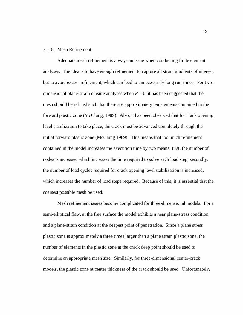
3-1-6 Mesh Refinement
Adequate mesh refinement is always an issue when conducting finite element
analyses. The idea is to have enough refinement to capture all strain gradients of interest,
but to avoid excess refinement, which can lead to unnecessarily long run-times. For two-
dimensional plane-strain closure analyses when R = 0, it has been suggested that the
mesh should be refined such that there are approximately ten elements contained in the
forward plastic zone (McClung, 1989). Also, it has been observed that for crack opening
level stabilization to take place, the crack must be advanced completely through the
initial forward plastic zone (McClung 1989). This means that too much refinement
contained in the model increases the execution time by two means: first, the number of
nodes is increased which increases the time required to solve each load step; secondly,
the number of load cycles required for crack opening level stabilization is increased,
which increases the number of load steps required. Because of this, it is essential that the
coarsest possible mesh be used.
Mesh refinement issues become complicated for three-dimensional models. For a
semi-elliptical flaw, at the free surface the model exhibits a near plane-stress condition
and a plane-strain condition at the deepest point of penetration. Since a plane stress
plastic zone is approximately a three times larger than a plane strain plastic zone, the
number of elements in the plastic zone at the crack deep point should be used to
determine an appropriate mesh size. Similarly, for three-dimensional center-crack
models, the plastic zone at center thickness of the crack should be used. Unfortunately,

20
this forces the mesh to have more than adequate refinement at the crack free surface, and
necessitates nearly three times as many load cycles for crack opening level stabilization
at the crack free surface. In view of this fact, for the semi-elliptical cracks modeled,
crack opening level stabilization attainment was achieved only at the crack deep point in
the current study. This was considered satisfactory because the experimentally
determined opening loads used for comparison with the finite element results were
limited to points away from the free surface.
Since plastic zone sizes are not known before the analyses, an approximation for
the plastic zone size must be used to estimate an appropriate mesh size. The equation
developed by Irwin (Grandt, 1984) is used:
2
0
1
=
σπαKrp (3.1)
where,
rp = crack forward plastic zone size
K = stress intensity factor under maximum load
σ0 = material yield stress
α = 1 for plane stress, 3 for plane strain
The mesh is then created with elemental length da ≈ 0.1 rp. The maximum load is
then applied statically to the model and the actual plastic zone size is checked to ensure
adequate refinement.
Because the suggested mesh refinement requirements in the open literature were
developed for two-dimensional models, a mesh refinement study for three-dimensional

21
models is performed in the current research. The suggested mesh refinement guidelines
for two-dimensional models are used as a starting point for the current work. The mesh
refinement study performed is discussed in a subsequent chapter.
3-2 Crack Closure Related Issues
3-2-1 Crack Advance
Modeling of plasticity-induced fatigue crack closure is essentially the same as
modeling the formation of a plastic wake near a crack front. This formation of a plastic
wake can be accomplished only by advancing the crack tip through the initial monotonic
crack plastic zone. In reality, crack advance takes place in very small increments over
several cycles. Unfortunately, the finite element requires this crack advance to be
discretized and to take place at a specific load. When using the finite element method
crack growth can take place only in integer multiples of the element length, da, at the
crack tip.
More importantly, however, is at what point during the load cycle should crack
advance take place. Many researchers suggest crack advance should take place at the
minimum load to aid in convergence (McClung, 1989). Other researchers, however,
suggest that crack advance at minimum load is physically unrealistic, since in reality
there are no mechanisms present to cause crack growth on a closed crack. Instead, they
suggest that crack advance should take place at the maximum load (Newman, 1976). In
the present studies, crack advance occurs at the maximum load, but to ease convergence
the crack front nodes are released incrementally. This is accomplished by determining

22
the crack front reaction forces present at maximum load. The crack front fixities are then
removed, and are replaced with a force that is a fraction of the reaction force. The force
is then gradually removed until it can be totally removed without convergence problems.
In the present work, the reaction force is bisected four times before being removed
completely. Also, it should be noted that in the current study crack advance is uniform
with each point on the crack front moving forward one element width perpendicular to
the crack front. Consequently, crack aspect ratios are fixed throughout the crack growth
process.
3-2-2 Crack Surface Contact
Now that the crack has the ability to advance and the plastic wakes forms, the
issue of crack surface contact must be addressed. In order to prevent the crack surfaces
from penetrating, some mechanism must be implemented in the finite element script.
There are several ways of accomplishing this, the simplest and most obvious is the use of
contact elements along the crack plane. However, convergence problems with contact
elements lead to very long run times. To keep the execution times reasonable, a different
method was needed.
An alternate method, which is used by Newman (Newman, 1976), is to monitor
the crack surface displacements. Once they become negative, a very large stiffness is
added to the diagonal of the assembled finite element stiffness matrix, which prevents
further penetration. This “spring” is removed when the crack surface begins to open
again on the subsequent loading. Unfortunately, since a commercial code (ANSYS) is
being used in the current study, a modification to the assembled stiffness matrix is
23
difficult. Instead, the following scheme is used. During loading and unloading, the
remote loads are changed by small load increments. At the end of each load increment,
the status of each of the crack surface nodes is checked. During unloading, the
displacement of each node is monitored. If the displacement becomes negative, a nodal
fixity is immediately applied preventing the node from further penetration. On the
subsequent loading, the reaction forces on all of the nodes on the crack surface that
closed are monitored. If the reaction forces on the nodes become positive (the node is in
tension), the nodal fixity is removed. The remote load at which the last nodal fixity is
removed is the crack opening load. Unfortunately, the opening load can be found only to
the resolution of the loading increment.
Remote Load
Nod
al R
eact
ion
Forc
e
Interpolated Opening Load
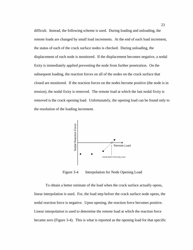
Figure 3-4 Interpolation for Node Opening Load
To obtain a better estimate of the load when the crack surface actually opens,
linear interpolation is used. For, the load step before the crack surface node opens, the
nodal reaction force is negative. Upon opening, the reaction force becomes positive.
Linear interpolation is used to determine the remote load at which the reaction force
became zero (Figure 3-4). This is what is reported as the opening load for that specific

24
node. The linear interpolation is executed using a FORTRAN code, closinterp, which
can be found in Appendix F.
3-3 Closure Model Overview
Now that all of the components of to the crack closure model have been
developed they can be combined. The following is a full overview of the entire crack
closure modeling process as is done in the current research.
Load Unload
Initial LoadIncrement
LoadIncrementwhileOpening
Final LoadIncrement
Initial UnloadIncrement
UnloadIncrementwhileClosing
Final UnloadIncrement
Smin
Smax
First NodeOpens
Last NodeOpens
First NodeCloses
Last NodeCloses
Load Step
Rem
ote
Load
CrackAdvance
Figure 3-5 Typical Load Cycle
Plasticity-induced fatigue crack closure is modeled by cyclically applying loads,
during which the crack is grown a small amount. Figure 3-5 shows the steps contained in
a typical load cycle. Initially a large load increment is used to save execution time. After
the first node on the crack surface opens, a smaller load increment is used until all the
nodes on the crack surface is open. A larger load increment is then used until the

25
maximum load is reached, at which point crack advance takes place. The first load step
of crack advance, the nodal fixities on the crack front are removed and are replaced by a
force equal to 50% of the node reaction forces. The forces are then reduced over three
additional load steps when they become near zero, after which they are completely
removed. The entire crack front has now advanced one elemental length perpendicular to
the crack front. Unloading then takes place. Similar to the loading, a large increment is
used initially, which is decreased when the crack begins to close and is increased again
after the entire crack surface has closed. These load cycles are repeated several times
until the crack opening levels reach stabilized values.

26
CHAPTER IV
PRELIMINARY SCRIPT VERIFICATION
To ensure the functionality of the developed ANSYS scripts, they are used to
make finite element predictions of crack opening levels in simple geometries that have
been completed independent of the current research. First, a two-dimensional plane
strain analysis is performed to allow comparison with the early work of Newman
(Newman, 1976). Next, a three dimensional analysis is performed to compare with
predictions made by Chermahini et al. (Chermahini, 1988) in a three dimensional center-
cracked geometry. Also, some additional comparisons are made with results obtained
using the finite element code Zip3d, which was designed for crack closure analyses and is
used by Chermahini et al.
4-1 Two Dimensional Verification
In order to ensure that the ANSYS script is working properly, a two-dimensional
finite element model is created in imitation of an analysis performed by Newman
(Newman, 1976). This was chosen as a starting point because the inherent simplicity in a
two-dimensional model as well as the quick run-time, allowing for quick debugging of
the script.
27
a
h
w
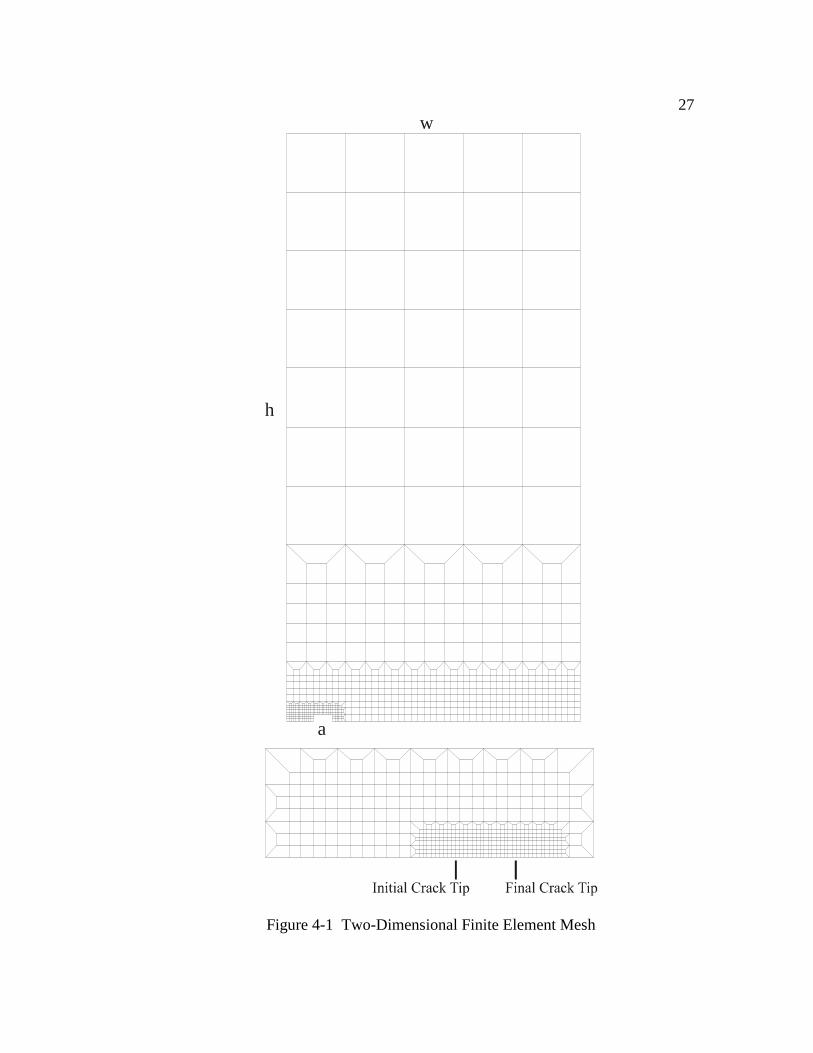
Figure 4-1 Two-Dimensional Finite Element Mesh
28
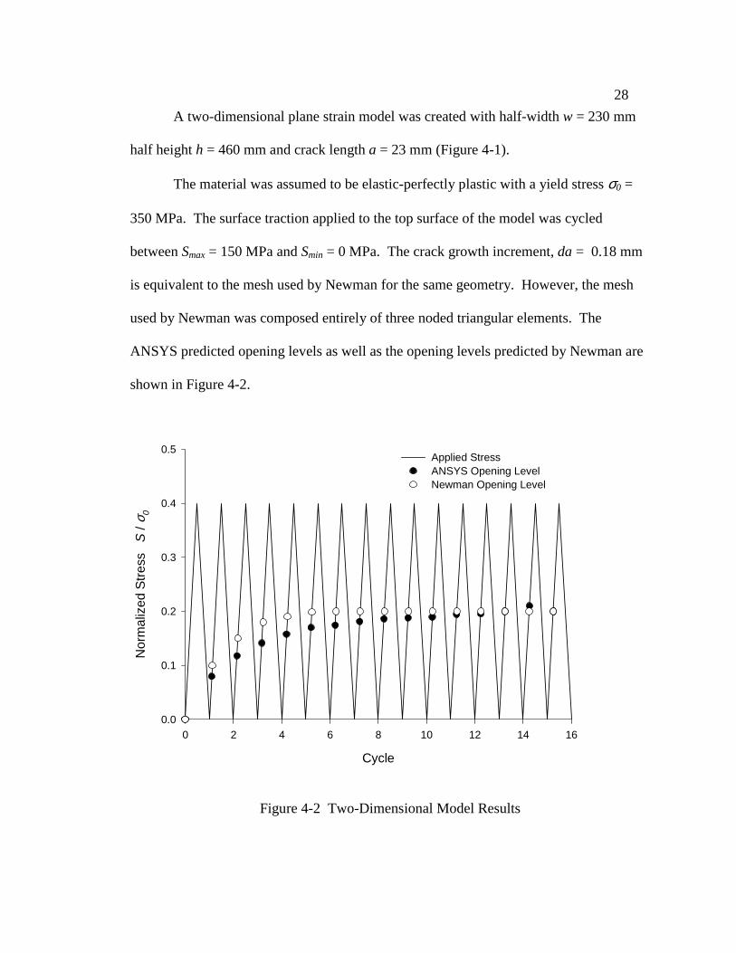
A two-dimensional plane strain model was created with half-width w = 230 mm
half height h = 460 mm and crack length a = 23 mm (Figure 4-1).
The material was assumed to be elastic-perfectly plastic with a yield stress σ0 =
350 MPa. The surface traction applied to the top surface of the model was cycled
between Smax = 150 MPa and Smin = 0 MPa. The crack growth increment, da = 0.18 mm
is equivalent to the mesh used by Newman for the same geometry. However, the mesh
used by Newman was composed entirely of three noded triangular elements. The
ANSYS predicted opening levels as well as the opening levels predicted by Newman are
shown in Figure 4-2.
Figure 4-2 Two-Dimensional Model Results
Cycle
0 2 4 6 8 10 12 14 16
Nor
mal
ized
Stre
ss
S / σ
0
0.0
0.1
0.2
0.3
0.4
0.5Applied StressANSYS Opening LevelNewman Opening Level

29
The stabilized ANSYS opening levels correlate well with the opening levels
calculated by Newman. The ANSYS scripts work sufficiently for the two-dimensional
model.
4-2 Three Dimensional Verification A three-dimensional model geometry and loading configuration was chosen to
match the analysis done by Chermahini et al. (Chermahini, 1988). Only minor
differences between the current model and Chermahini’s model exist, the main difference
being more element refinement through the thickness of the current model.
The center-cracked panel was modeled using three planes of symmetry. The
model was given a half-width, w = 40 mm, a half-thickness, t = 2.39 mm, and a half-
height, h = 80 mm. The initial crack half-length was a = 19.7 mm, which was extended
by one element length (da = 0.003 mm) every growth cycle. This mesh is comprised of 6
elemental layers with a total of 5,706 solid brick elements and 7,203 nodes (Figure 4-3).
The material properties used in this model are equivalent to those of an aluminum
alloy. The material was assumed to be elastic, perfectly-plastic with a yield stress, σ0, =
345 MPa, and a modulus of elasticity E = 70,000 MPa. The model was subjected to
constant amplitude loading with Smax = 86.25x10⁶ MPa and Smin = 0.0 MPa. Each loading
and unloading was subdivided into 20 substeps, giving a maximum resolution on opening
and closing values equal to 5% of Smax. A total of 20 complete loading cycles were
performed, which is equivalent to 800 consecutive static analyses. Because the large
number of analyses performed on a relatively small number of degrees of freedom, the
frontal direct solver was used for the analysis.
30
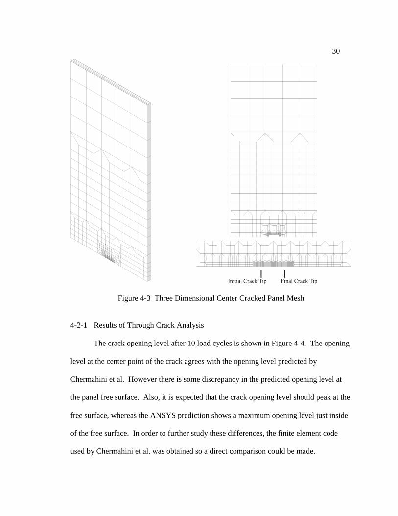
Figure 4-3 Three Dimensional Center Cracked Panel Mesh
4-2-1 Results of Through Crack Analysis
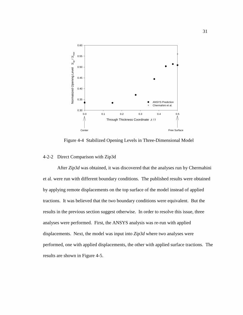
The crack opening level after 10 load cycles is shown in Figure 4-4. The opening
level at the center point of the crack agrees with the opening level predicted by
Chermahini et al. However there is some discrepancy in the predicted opening level at
the panel free surface. Also, it is expected that the crack opening level should peak at the
free surface, whereas the ANSYS prediction shows a maximum opening level just inside
of the free surface. In order to further study these differences, the finite element code
used by Chermahini et al. was obtained so a direct comparison could be made.
31
Through Thickness Coordinate z / t
0.0 0.1 0.2 0.3 0.4 0.5
Nor
mal
ized
Ope
ning
Lev
el
Sop
/ S
max
0.30
0.35
0.40
0.45
0.50
0.55
0.60
X
X
ANSYS PredictionChermahini et al.X
Center Free Surface
Figure 4-4 Stabilized Opening Levels in Three-Dimensional Model 4-2-2 Direct Comparison with Zip3d
After Zip3d was obtained, it was discovered that the analyses run by Chermahini
et al. were run with different boundary conditions. The published results were obtained
by applying remote displacements on the top surface of the model instead of applied
tractions. It was believed that the two boundary conditions were equivalent. But the
results in the previous section suggest otherwise. In order to resolve this issue, three
analyses were performed. First, the ANSYS analysis was re-run with applied
displacements. Next, the model was input into Zip3d where two analyses were
performed, one with applied displacements, the other with applied surface tractions. The
results are shown in Figure 4-5.

32
0.0 0.1 0.2 0.3 0.4 0.5
Nor
mal
ized
Ope
ning
Lev
el
S op /
S max
0.30
0.35
0.40
0.45
0.50
0.55
0.60
0.65
Zip 3d (Applied Displacments)Zip 3d (Applied Pressure)Ansys (Applied Displacement)Ansys (Applied Pressure)
Through Thickness Coordinate z / t
Center Free Surface
Figure 4-5 Remote Boundary Condition Effects
These results show good agreement between ANSYS and zip3d. This suggests
that the closure scripts for ANSYS are working properly and can now be applied to the
more complicated surface crack models. Also, the results suggest that the choice of
remote boundary conditions may have an effect on the results near the free surface. The
choice of applied displacements vs. applied surface tractions will be investigated for the
surface crack in the following chapter. It seems logical, however, that if the two are
equivalent in an un-cracked geometry, then they will be nearly equivalent in a body with
small cracks. The previous analyses may have exaggerated the effects since such a long
crack (a/t = 0.5) was being investigated.

33
CHAPTER V
MODELING PARAMETER EFFECTS
Since the ANSYS closure script has been shown to be working properly. An
investigation will now be made into the effects of the various modeling parameters. First
will be an investigation of the ANSYS specific parameters: the equation solver tolerance
and the use of non-linear solution control. Next will be the more general parameter
studies including a mesh refinement study and the effects of changing the load increment,
using a large deformation constitutive equation, changing the applied boundary
conditions, and incorporating material strain hardening. For brevity, these effects will be
investigated on only one model. All of the parameter effects will be investigated on a
surface crack geometry.
The model that will be used is a circular surface crack model with R = 0 which
has a high applied stress ratio Smax / σ0 = 0.7 to minimize the meshing requirements. The
model was generated with height h = 25.4 mm, half-width w = 12.7 mm, thickness t =
12.7 mm, crack depth a = 1.27 mm, and a crack half-length c = 1.27 mm (Figure 5-1).
Two planes of symmetry were utilized requiring only one quarter of the model to be
meshed. The mesh containing 16023 nodes and 14033 elements was built using the
program scpcell, made available by R. H. Dodds of the University of Illinois.

34
S
S
A
A
φa
t
c
w
2w
Section -A A
H
h
a
w
t
c
h
Figure 5-1 Model Used for Parameter Studies
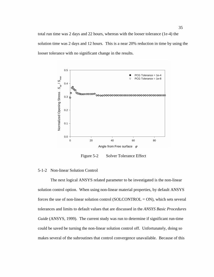
5-1 ANSYS Specific Parameters 5-1-1 Equation Solver Tolerance
The first parameter to be investigated is the solver tolerance on the Pre-
Conditioned Conjugate Gradient (PCG) solver. This solver is the most robust for solid
models with more than 50,000 degrees of freedom. The default tolerance on the solver is
1e-8. An analysis is performed with the tolerance loosened to 1e-4 to determine if a
looser tolerance will give equivalent results and also determine the amount of time saved.
Five load cycles are modeled on the surface crack geometry described above and the
opening levels are compared for the two solver tolerances in Figure 5-2. The crack
opening levels obtained are nearly identical. This suggests that the looser tolerance can
be used without compromising the results. With the default solver tolerance (1e-8), the
35
total run time was 2 days and 22 hours, whereas with the looser tolerance (1e-4) the
solution time was 2 days and 12 hours. This is a near 20% reduction in time by using the
looser tolerance with no significant change in the results.
Angle from Free surface φ
0 20 40 60 80
Nor
mal
ized
Ope
ning
Stre
ss
S op /
S max
0.0
0.1
0.2
0.3
0.4
0.5
PCG Tolerance = 1e-4PCG Tolerance = 1e-8
Figure 5-2 Solver Tolerance Effect
5-1-2 Non-linear Solution Control
The next logical ANSYS related parameter to be investigated is the non-linear
solution control option. When using non-linear material properties, by default ANSYS
forces the use of non-linear solution control (SOLCONTROL = ON), which sets several
tolerances and limits to default values that are discussed in the ANSYS Basic Procedures
Guide (ANSYS, 1999). The current study was run to determine if significant run-time
could be saved be turning the non-linear solution control off. Unfortunately, doing so
makes several of the subroutines that control convergence unavailable. Because of this

36
the results became very poor after just one load cycle. The nodal displacements of the
row of nodes directly behind the crack front after the first increment of unloading on the
first cycle are shown in Figure 5-3. It is clear that the results with the non-linear solution
control are much better behaved. A successful analysis without non-linear solution
control was never attained.. For this reason non-linear solution control is used for all the
subsequent analyses.
Angle from Free Surface φ
0 20 40 60 80
Nod
al D
ispl
acem
ent
Uy
(in)
0
5e-6
1e-5
2e-5
2e-5
3e-5
3e-5
SOLCONTROL OFFSOLCONTROL ON
Figure 5-3 Non-Linear Solution Control
5-2 General Checks 5-2-1 Mesh Refinement Study
A mesh refinement study was performed on the mesh described above. Three
different meshes were used with elemental lengths, da = 0.003175 mm, 0.00635 mm, and
0.0127 mm. These meshes contained 20, 10, and 5 elements in the forward plastic zone

37
respectively. These analyses showed that if an equal amount of crack growth is
considered, equivalent results are obtained at both the deep point and the free surface for
the two coarser meshes (Figure 5-4). This suggests that five elements in the forward
plastic zone at the crack deep point is adequate. The analysis for the most refined mesh
was inconclusive because due to the large computational time required, only four load
cycles were completed.
Crack Growth ∆a, ∆c, mm
0.00 0.01 0.02 0.03 0.04 0.05 0.06 0.07
Nor
mal
ized
Ope
ning
Stre
ss
S op /
S max
0.10
0.15
0.20
0.25
0.30
0.35
0.40
0.45
Mesh 1 Free SurfaceMesh 1 Deep PointMesh 2 Free SurfaceMesh 2 Deep PointMesh 3 Free SurfaceMesh 3 Deep Point
Figure 5-4 Mesh Refinement Study 5-2-2 Load Increment Effect
Since the nodal contact status with the crack plane on the crack surface is being
monitored only at finite load increments during the loading and unloading portions of the
load cycles, it seems natural to ask how small a load increment is necessary. A very
small load increment would probably give very good results, but require long
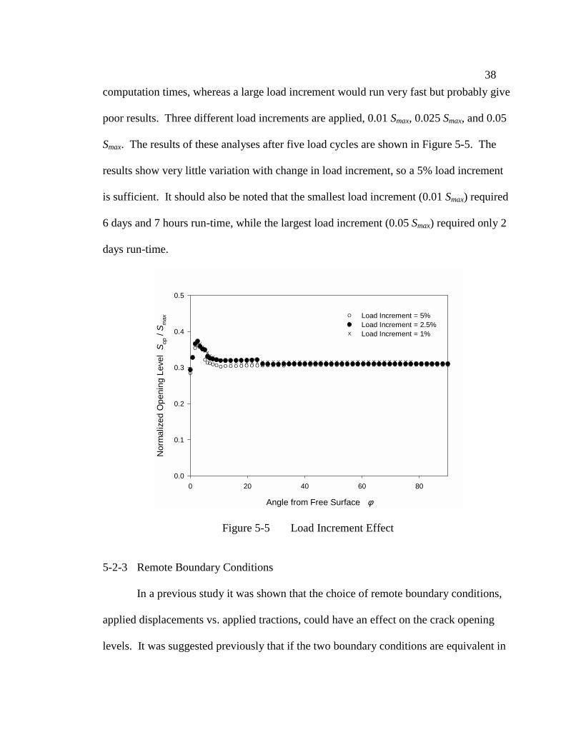
38
computation times, whereas a large load increment would run very fast but probably give
poor results. Three different load increments are applied, 0.01 Smax, 0.025 Smax, and 0.05
Smax. The results of these analyses after five load cycles are shown in Figure 5-5. The
results show very little variation with change in load increment, so a 5% load increment
is sufficient. It should also be noted that the smallest load increment (0.01 Smax) required
6 days and 7 hours run-time, while the largest load increment (0.05 Smax) required only 2
days run-time.
Angle from Free Surface φ
0 20 40 60 80
Nor
mal
ized
Ope
ning
Lev
el S
op /
S max
0.0
0.1
0.2
0.3
0.4
0.5
OOOOOOOOOOOOOOOOOOOOOOOOOOOOOOOOOOOOOOOOOOOOOOOOO
OOOO
O
O
XXXXXXXXXXXXXXXXXXXXXXXXXXXXXXXXXXXXXXXXXXXXXXXXXXXXX
X
X
Load Increment = 5%O
Load Increment = 2.5%Load Increment = 1%X
Figure 5-5 Load Increment Effect
5-2-3 Remote Boundary Conditions
In a previous study it was shown that the choice of remote boundary conditions,
applied displacements vs. applied tractions, could have an effect on the crack opening
levels. It was suggested previously that if the two boundary conditions are equivalent in

39
an un-cracked geometry they should be equivalent in a geometry with a short crack
(where the compliance of the cracked geometry is nearly the same as the un-cracked
geometry). To check this assumption both sets of boundary conditions are applied to the
model described above. The results are shown in Figure 5-6. There is very little effect
on the opening behavior for this geometry with the different boundary conditions. This
may be different for deeper surface cracks, but for the remaining analyses applied
tractions will be utilized.
Angle from Free Surface φ
0 20 40 60 80
Nor
mal
ized
Ope
ning
Stre
ss S
op /
S max
0.0
0.1
0.2
0.3
0.4
0.5
Applied DisplacmentsApplied Tractions
Figure 5-6 Effect of Remote Boundary Conditions
5-2-4 Large Deformation Effects
In a cracked body under load very large deflections and rotations are present in
the vicinity of the crack tip (Swedlow, 1986). These large deflections change the
differential equations of the body, and force more complicated non-linear solution

40
algorithms. This geometric non-linearity is typically ignored, but since a commercial
finite element package is being used which has built in the capability of solving non-
linear geometry problems its effect on crack closure can be determined. The model
described above was again solved incorporating the non-linear geometry effects option in
ANSYS. The results after five growth cycles are shown in Figure 5-7. The non-linear
geometry algorithm had little effect on the results, with the exception of a significant
increase in run-time (approximately by a factor of 1.5).
Angle from Free Surface φ
0 20 40 60 80
Nor
mal
ized
Ope
ning
Stre
ss
S op /
S max
0.25
0.30
0.35
0.40
0.45
0.50
OOOOOOOOOOOOOOOOOOOOOOOOOOOOOOOOOOOOOOOOOOOOOOOO
O
OOO
O
O
O
NLGEOM ONO
NLGEOM OFF
Figure 5-7 Large Deformation Effects
5-2-5 Strain Hardening
A strain hardening study was next performed. A bi-linear material model with
kinematic hardening was used with tangent modulus H = 0.0 E, 0.1 E, and 0.2 E, where E

41
is the elastic modulus. The results showed a significant decrease in the crack opening
levels when hardening is present (Figure 5-8).
While a significant decrease in opening levels was predicted with increased strain
hardening, hardening was not used in the current study because several new modeling
issues are introduced. Principal among these new issues is the Bauschinger effect and its
impact on crack closure. From a finite element analysis perspective, the consideration of
the Bauschinger effect is restricted to employing either isotropic or kinematic hardening,
both of which are idealizations. Using kinematic hardening will approximate the
Bauschinger effect, and the use of isotropic hardening neglects the effect completely.
Hardening may also affect plastic zone sizes, and hence affect mesh refinement
requirements.
Parametric Angle φ
0 20 40 60 80
Nor
mal
ized
Ope
ning
Stre
ss
S op /
S max
0.0
0.1
0.2
0.3
0.4
0.5
0.6
H / E = 0.0H / E = 0.1H / E = 0.2
Figure 5-8 Strain Hardening Effects

42
5-3 Summary
A number of different model parameters were investigated in the current study.
Many of the parameters did not make a difference in the solution, but gave significant
savings in run-time. This was the case for the PCG equation solver tolerance, which was
found to be sufficient at 1e-4 with a time savings of nearly 20%. Also, a larger load
increment (5% of the load range) can be used to reduce the number of load steps and run-
time without affecting the accuracy of the results. Also, these checks provided insight
into some of the options that may be necessary for an accurate analysis. The non-linear
solution control option in ANSYS is essential in obtaining converged results, while the
large deformation effects option is unnecessary. Lastly, the effect of material strain
hardening was shown to be significant. Higher levels of strain hardening resulted in
lower opening levels.
43
CHAPTER VI
COMPARISON WITH EXPERIMENTAL RESULTS
One of the objectives of this research is to compare finite element predictions
with experimental results. Unfortunately, measuring opening stresses in semi-elliptical
surface flaws is extremely difficult, and typical methods relying on remote displacement
curves cannot be used to measure local opening levels. Instead, fracture surfaces can be
used to indirectly determine opening levels from striation spacing patterns. This is the
method that was used by Putra and Schijve (Putra, 1992), and it is these results that will
be used for comparison.
Putra and Schijve published opening load measurements from five different
aluminum alloy (7075-T6) specimens under uniaxial loading with R = 0.1, each with a
unique initial aspect ratio. For each specimen, results were published for four different
crack depths. Because of the large solution times required for small amounts of crack
growth, no attempt was made to model the growth of a crack from its initial crack length.
Consequently, aspect ratio evolution was not modeled. Instead, finite element meshes
were made for each of the experimental specimens at the crack depths for which data
were published. The aspect ratios used in making the finite element meshes were taken
from the aspect ratios measured experimentally.

44
6-1 Finite Element Model Descriptions
There was a possibility of twenty different analyses, each with a corresponding
published experimental result. However, due to the long execution times required for
each model, only three of the published specimens were used. The specimens with an
initial aspect ratio (a/c)i of 0.2, 0.4 and 1.0 were chosen. The number of analyses was
further reduced by convergence problems with deep cracks (a / t > 0.8) leaving only ten
geometries to be analyzed (Table 6-1). The specimen half-height h = 50 mm, thickness t
= 9.6 mm, and half-width w = 50 mm remained constant for all the models. The applied
uniaxial tractions were Smax = 150 MPa and Smin = 15 MPa with Smax/σ0 = 0.27. The
modulus of elastitity and poisson’s ratio used were E = 69,980 MPa and ν = 0.3. As
before, two planes of symmetry were utilized requiring only ¼ of the specimen to be
modeled (Figure 6-1). Also, the number of degrees of freedom (3 per node) was kept
below 100,000 to minimize execution time. All of the meshes had at least five elements
in the forward plastic zone (rp/da > 5) at the crack deep point, which was shown
previously to be adequate. All models were run for ten crack growth cycles.
Table 6-1 Models used to compare with experimental data.
Specimen a/t a c da rp/da Nodes Elements PCA 06 0.31 2.976 9.525 0.005 8 33479 29828
(a/c)i = 0.2 0.55 5.28 10.429 0.005 15 30333 26972 0.66 6.336 11.568 0.005 22 32927 29340 0.78 7.488 13.057 0.005 26 25498 32622
PCA 13 0.34 3.264 3.3 0.0025 6 26079 23016 (a/c)i = 1.0 0.53 5.88 5.7 0.0025 18 36440 32730
0.71 6.816 8.125 0.005 11 28222 25020 PCA 15 0.38 3.6605 7.412 0.005 8 59493 53504
(a/c)i = 0.4 0.48 4.6305 8.1225 0.005 10 33047 29440 0.59 5.664 9.005 0.005 14 36044 32196
45
xy
z
h = 50 mm
a
c
t = 9.6 mm
w = 50 mm
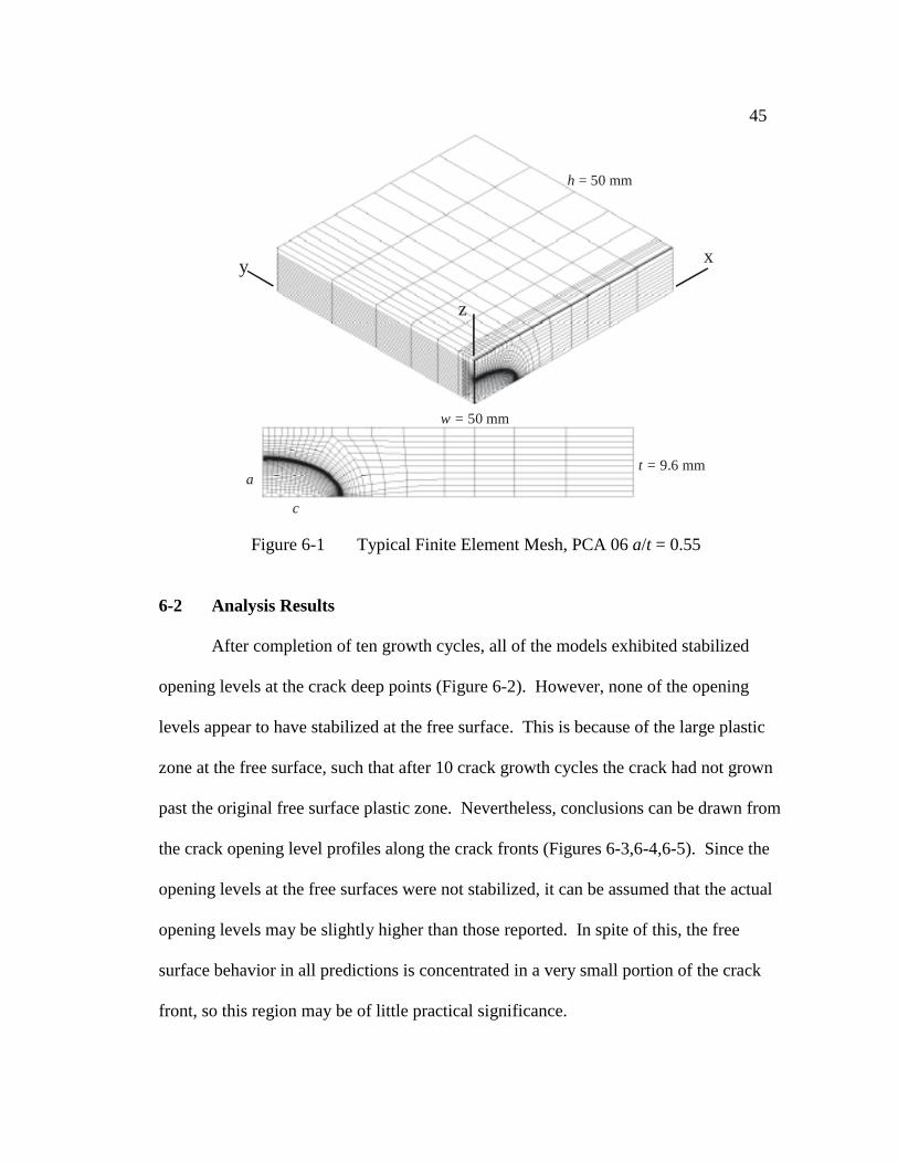
Figure 6-1 Typical Finite Element Mesh, PCA 06 a/t = 0.55
6-2 Analysis Results
After completion of ten growth cycles, all of the models exhibited stabilized
opening levels at the crack deep points (Figure 6-2). However, none of the opening
levels appear to have stabilized at the free surface. This is because of the large plastic
zone at the free surface, such that after 10 crack growth cycles the crack had not grown
past the original free surface plastic zone. Nevertheless, conclusions can be drawn from
the crack opening level profiles along the crack fronts (Figures 6-3,6-4,6-5). Since the
opening levels at the free surfaces were not stabilized, it can be assumed that the actual
opening levels may be slightly higher than those reported. In spite of this, the free
surface behavior in all predictions is concentrated in a very small portion of the crack
front, so this region may be of little practical significance.

46
PCA 06a / t = 0.66
0.0
0.1
0.2
0.3
0.4
0.5
0.6
PCA 13a / t = 0.53
PCA 15a / t = 0.48
normalized crack depth growth ∆a/da
PCA 15a / t = 0.59
0 2 4 6 8 10
PCA 06a / t = 0.55
0.0
0.1
0.2
0.3
0.4
0.5
0.6
PCA 06a / t = 0.31
0.0
0.1
0.2
0.3
0.4
0.5
0.6
Free SurfaceDeep Point
PCA 13a / t = 0.34
norm
aliz
ed o
peni
ng s
tress
S o
p / S
max
PCA 06a / t = 0.78
0 2 4 6 8 100.0
0.1
0.2
0.3
0.4
0.5
0.6
PCA 15a / t = 0.38
PCA 13a / t = 0.71
0 2 4 6 8 10
Figure 6-2 Crack Opening Level Stabilization
47
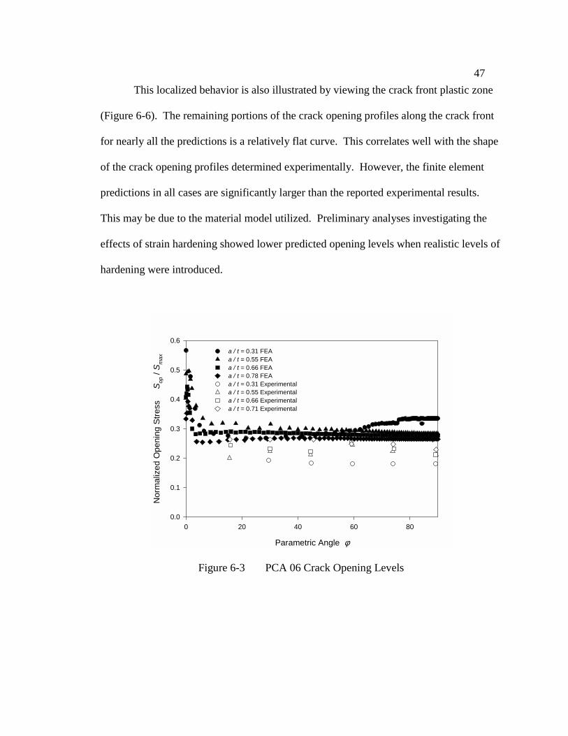
This localized behavior is also illustrated by viewing the crack front plastic zone
(Figure 6-6). The remaining portions of the crack opening profiles along the crack front
for nearly all the predictions is a relatively flat curve. This correlates well with the shape
of the crack opening profiles determined experimentally. However, the finite element
predictions in all cases are significantly larger than the reported experimental results.
This may be due to the material model utilized. Preliminary analyses investigating the
effects of strain hardening showed lower predicted opening levels when realistic levels of
hardening were introduced.
Parametric Angle φ
0 20 40 60 80
Nor
mal
ized
Ope
ning
Stre
ss
Sop
/ S
max
0.0
0.1
0.2
0.3
0.4
0.5
0.6a / t = 0.31 FEAa / t = 0.55 FEAa / t = 0.66 FEAa / t = 0.78 FEAa / t = 0.31 Experimentala / t = 0.55 Experimentala / t = 0.66 Experimentala / t = 0.71 Experimental
Figure 6-3 PCA 06 Crack Opening Levels

48
Parametric Angle φ
0 20 40 60 80
Nor
mal
ized
Ope
ning
Stre
ss
Sop
/ S
max
0.0
0.1
0.2
0.3
0.4
0.5
0.6
a / t = 0.34 FEAa / t = 0.53 FEAa / t = 0.71 FEAa / t = 0.34 Experimentala / t = 0.53 Experimentala / t = 0.71 Experimental
Figure 6-4 PCA 13 Crack Opening Levels
Parametric Angle φ
0 20 40 60 80
Nor
mal
ized
Ope
ning
Stre
ss
Sop
/ S m
ax
0.0
0.1
0.2
0.3
0.4
0.5
0.6
a / t = 0.38 FEAa / t = 0.48 FEAa / t = 0.59 FEAa / t = 0.38 Experimentala / t = 0.48 Experimentala / t = 0.59 Experimental
Figure 6-5 PCA 15 Crack Opening Levels
49
y / c0.0 0.2 0.4 0.6 0.8 1.0
x / a
0.0
0.2
0.4
0.6
0.8
1.0
crack frontplastic zone boundary
y / c0.8 0.9 1.0
x / a
0.0
0.1
0.2
0.3
0.4
0.5
crack frontplastic zone boundary
Figure 6-6 Typical Plastic Zone
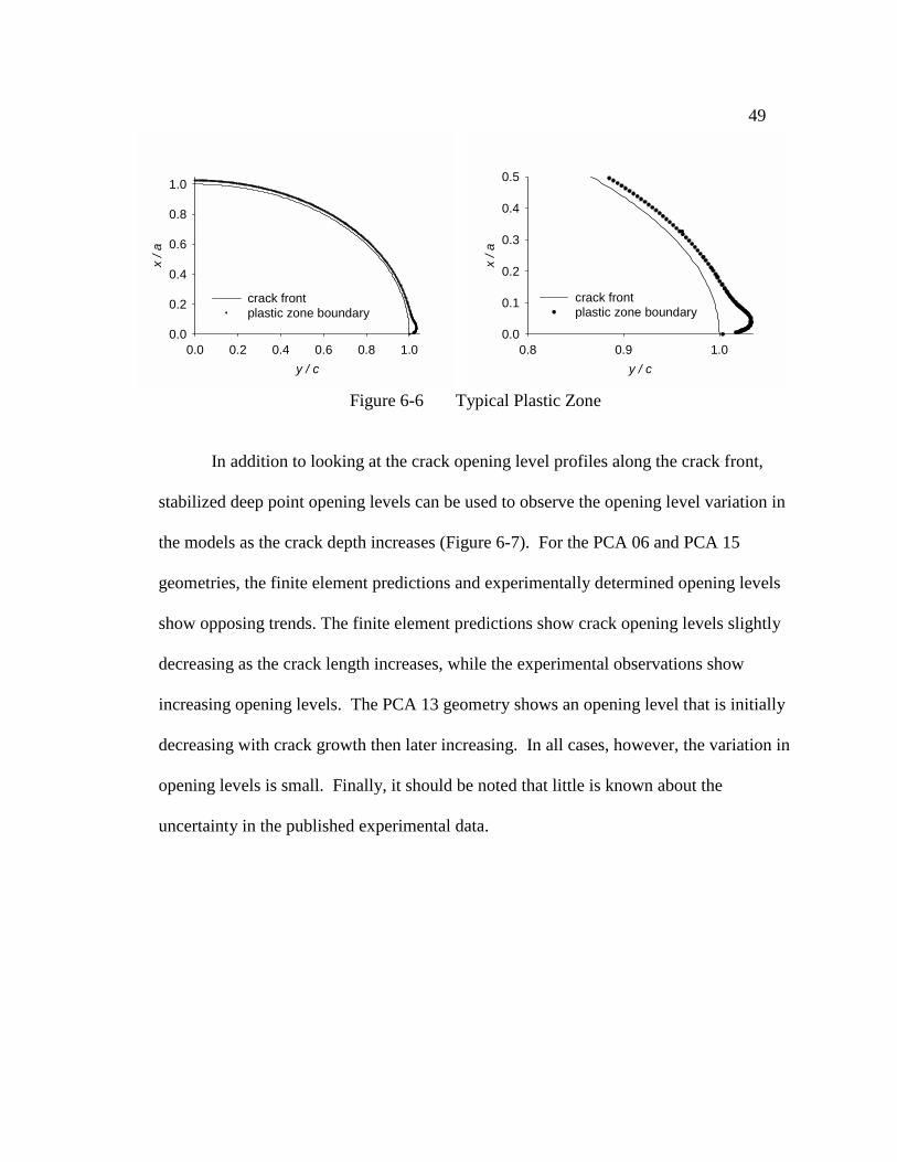
In addition to looking at the crack opening level profiles along the crack front,
stabilized deep point opening levels can be used to observe the opening level variation in
the models as the crack depth increases (Figure 6-7). For the PCA 06 and PCA 15
geometries, the finite element predictions and experimentally determined opening levels
show opposing trends. The finite element predictions show crack opening levels slightly
decreasing as the crack length increases, while the experimental observations show
increasing opening levels. The PCA 13 geometry shows an opening level that is initially
decreasing with crack growth then later increasing. In all cases, however, the variation in
opening levels is small. Finally, it should be noted that little is known about the
uncertainty in the published experimental data.

50
Normalized Crack Depth a / t
0.2 0.3 0.4 0.5 0.6 0.7 0.8 0.9
Nor
mal
ized
Ope
ning
Stre
ss
Sop
/ S m
ax
0.0
0.1
0.2
0.3
0.4
0.5
0.6
PCA 06 FEAPCA 06 ExperimentalPCA 13 FEAPCA 13 ExperimentalPCA 15 FEAPCA 15 Experimental
Figure 6-7 Comparison of Stabilized Deep Point Opening Levels
6-3 Conclusions Finite element analysis was used to predict crack opening levels in part-through
semi-elliptical surface flawed geometries. These predictions were compared with
published experimental data. Previous mesh refinement studies showed that five
elements in contained in the forward plastic zone is adequate. All the models in the
current study contained adequate refinement by this criterion. For nearly all geometries,
the crack opening level profile along the crack front correlated well with the
experimentally determined profiles. However, in all cases the finite element predictions
gave opening levels significantly higher than those determined experimentally. This may
be a consequence of the constitutive model employed, which neglected strain hardening.
For all predictions there was a variation in the opening level profile due to the free
surface, but this was concentrated in that portion of the crack front within 5 degrees of

51
the crack free surface. Thus, the lack of opening level stabilization observed at the crack
free surfaces may be of little practical significance. The prediction of the crack opening
level as the crack increases in depth was also compared with the experimental data. The
finite element predictions were seen to frequently contradict subtle trends that were
observed experimentally. However, since little is known about the uncertainty in the
experimental measurements, it is difficult for any conclusions to be drawn.
While the current study presented several sets of predictions for semi-elliptical
surface flaws, there is still much work necessary to characterize fatigue crack opening
levels in these types of geometries. The current study did not predict crack aspect
evolution based on crack opening levels. Eventually, a model should be created in which
crack opening levels are used to constantly evolve a crack aspect ratio, and more work
still needs to be done to characterize the effects of strain hardening on crack opening
levels.

52
CHAPTER VII
SUMMARY AND CONCLUSIONS
A script was developed in the finite element code ANSYS to model plasticity-
induced fatigue crack closure. The functionality of this script was tested by comparing
predicted crack opening levels with opening levels published opening levels obtained
from similar finite element routines. This verification included both a two-dimensional
and a three-dimensional center-cracked geometry. Similar results to those published
were obtained in both cases.
7-1 Parameter Study
Upon completion of the verification of the script, a parameter study was
performed in which the use of various finite element options was investigated. A
reduction to the default iterative solver tolerance resulted in accurate results with a run-
time savings of near 20%. Similarly, a load increment as large as 5% can be used
without compromising the accuracy of the results, which also results in significant run-
time savings. The use of the large deformation effects option was proven to be
inappropriate, and non-linear solution control was essential for convergence. Also, a
mesh refinement study was performed which showed that five element contained in the
crack forward plastic zone is adequate. Lastly, an investigation into the effects of strain

53
hardening was performed, where a significant decrease in crack opening levels was
predicted with increasing strain hardening.
7-2 Comparison with Experimental Results
Finite element predictions were made for three-dimensional semi-elliptical
surface cracked geometries to compare with published experimental data. For nearly all
the geometries investigated, the crack opening level profile along the crack front
correlated well with the experimentally determined profiles. However, in all cases the
finite element predictions yielded opening levels that were significantly higher than those
determined experimentally, which may be due the constitutive model employed which
neglected strain hardening. Also, the prediction of the variation in crack opening levels
as a function of crack depth was investigated and compared with the experimental data.
The finite element predictions were seen to frequently contradict subtle trends that were
observed experimentally. However, it is difficult for any conclusions to be drawn
because little is known about the uncertainty in the experimental measurements.
7-3 Recommended Future Work In the past, the finite element method has been used extensively in modeling
plasticity-induced fatigue crack closure in two-dimensional geometries, however more
work still needs to be done for three dimensional modeling efforts. Because of the large
expense of large three-dimensional models, very little research has been done in the past
on modeling fatigue crack closure in semi-elliptical flaws. More work should be done in
characterizing a mesh refinement criterion for these geometries, as well as further

54
investigating the effects of constitutive model employed. Further, the effects of variable
amplitude loading (i.e. spike overloads and block loading) should be investigated in
three-dimensional models since it is in these type loads that plasticity-induced crack
closure crack growth behavior. Also, a model should be developed that constantly
evolves a surface crack geometry while changing the crack aspect ratio from the variation
in opening levels along the crack front.
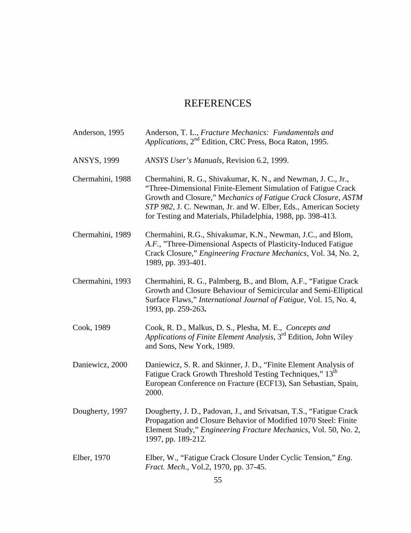
55
REFERENCES Anderson, 1995 Anderson, T. L., Fracture Mechanics: Fundamentals and
Applications, 2nd Edition, CRC Press, Boca Raton, 1995. ANSYS, 1999 ANSYS User’s Manuals, Revision 6.2, 1999. Chermahini, 1988 Chermahini, R. G., Shivakumar, K. N., and Newman, J. C., Jr.,
“Three-Dimensional Finite-Element Simulation of Fatigue Crack Growth and Closure,” Mechanics of Fatigue Crack Closure, ASTM STP 982, J. C. Newman, Jr. and W. Elber, Eds., American Society for Testing and Materials, Philadelphia, 1988, pp. 398-413.
Chermahini, 1989 Chermahini, R.G., Shivakumar, K.N., Newman, J.C., and Blom,
A.F., ”Three-Dimensional Aspects of Plasticity-Induced Fatigue Crack Closure,” Engineering Fracture Mechanics, Vol. 34, No. 2, 1989, pp. 393-401.
Chermahini, 1993 Chermahini, R. G., Palmberg, B., and Blom, A.F., “Fatigue Crack
Growth and Closure Behaviour of Semicircular and Semi-Elliptical Surface Flaws,” International Journal of Fatigue, Vol. 15, No. 4, 1993, pp. 259-263.
Cook, 1989 Cook, R. D., Malkus, D. S., Plesha, M. E., Concepts and
Applications of Finite Element Analysis, 3rd Edition, John Wiley and Sons, New York, 1989.
Daniewicz, 2000 Daniewicz, S. R. and Skinner, J. D., “Finite Element Analysis of
Fatigue Crack Growth Threshold Testing Techniques,” 13th European Conference on Fracture (ECF13), San Sebastian, Spain, 2000.
Dougherty, 1997 Dougherty, J. D., Padovan, J., and Srivatsan, T.S., “Fatigue Crack
Propagation and Closure Behavior of Modified 1070 Steel: Finite Element Study,” Engineering Fracture Mechanics, Vol. 50, No. 2, 1997, pp. 189-212.
Elber, 1970 Elber, W., “Fatigue Crack Closure Under Cyclic Tension,” Eng.
Fract. Mech., Vol.2, 1970, pp. 37-45.

56
Grandt, 1984 Grandt, A. F., Jr., “Introduction to Damage Tolerant Analysis Methodology,” Damage Tolerance of Metallic Structures: Analysis Methods and Applications, ASTM STP 842, J. B. Chang and J. L. Rudd, Eds., American Society for Testing and Materials, 1984, pp. 3-24.
McClung, 1989a McClung, R. C. and Sehitoglu, H., “On the Finite Element
Analysis of Fatigue Crack Closure-1. Basic Modeling Issues,” Engineering Fracture Mechanics, Vol. 33, No. 2, 1989, pp.237-252.
McClung 1989b McClung, R. C. and Sehitoglu, H., “On the Finite Element
Analysis of Fatigue Crack Closure-2. Numerical Results,” Engineering Fracture Mechanics, Vol. 33, No. 2, 1989, pp.253-272.
McClung, 1991 McClung, R. C., “Crack Closure and Plastic Zone Sizes in
Fatigue,” Fatigue and Fracture in Engineering Materials and Structures, Vol. 14, No. 4, 1991, pp. 455-468.
McClung, 1999 McClung, R. C., “Finite Element Analysis of Fatigue Crack
Closure: A Historical and Critical Review,” Fatigue ’99: The Seventh International Fatigue Conference, Beijing, China, 1999.
Newman, 1976 Newman, J. C., Jr., “A Finite-Element Analysis of Fatigue Crack
Closure,” Mechanics of Crack Growth, ASTM STP 590, American Society for Testing and Materials, 1976, pp. 281-301.
Park, 1997 Park, S. J., Earmme and Y. Y., Song, J. H., “Determination of the
Most Appropriate Mesh Size for 3-D Finite Element Analysis of Fatigue Crack Closure Behaviour,” Fatigue and Fracture in Engineering Materials and Structures, Vol. 20, No. 4, 1997, pp. 533-545.
Putra, 1992 Putra, I. S. and Schijve, J., “Crack Opening Stress Measurements
of Surface Cracks in 7075-T6 Aluminum Alloy Plate Specimen through Electron Fractography,” Fatigue and Fracture in Engineering Materials and Structures, Vol. 15, No. 4, 1992, pp. 323-338.
Reed, 1983 Redd, R. P., Smith, J. H., and Christ, B. W., “The Economic
Effects of Fracture in the United States,” U. S. Department of Commerce, National Bureau of Standards, Special Publication 647, March, 1983.

57
Rice, 1967 Rice, J. R., “Mechanics of Crack Tip Deformation and Extension
by Fatigue,” Fatigue Crack Propogation, ASTM STP 415, American Society for Testing and Materials, 1967, p. 247-311
Ridell, 1999 Riddell, W. T., Piascik, R. S., Sutton, M. A., Zhao, W., McNeill,
S.R., and Helm, J. D., “Determining Fatigue Crack Opening Loads from Near-Crack-Tip Displacement Measurements,” Advances in Fatigue Crack Closure Measurement and Analysis: Second Volume, ASTM STP 1343, R. C. McClung and J. C. Newman, Jr., Eds., American Society for Testing and Materials, West Conshohocken, PA, 1999, pp. 157-174.
Seshadri, 1995 Seshadri, B. R., Numerical Simulation and Experimental
Correlation of Crack Closure Phenomenon under Cyclic Loading, Ph.D., Dissertation, Indian Institute of Science, Bangalore, 1995.
Stephens, 2001 Stephens, R. I., Fatemi, A., Stephens, R. R., Fuchs, H. O., Metal
Fatigue in Engineering, 2nd Edition, John Wiley & Sons, Inc., New York, 2001.
Swedlow, 1986 Swedlow, J. L., “Computational Methods in Elastic-Plastic
Fracture Mechanics,” Wu, 1996 Wu, J and Ellyin, F., “A Study of Fatigue Crack Closure by
Elastic-Plastic Finite Element Analysis for Constant-Amplitude Loading,” International Journal of Fracture, Vol. 82, 1996, pp. 43-65.
Zhang, 1998 Zhang, J. Z. and Bowen, P., “On the Finite Element Simulation of
Three-Dimensional Semi-Circular Fatigue Crack Growth and Closure,” Engineering Fracture Mechanics, Vol. 60, No. 3, 1998, pp. 341-360.

58
APPENDIX A1
ANSYS INPUT FILE APPBCS.MAC
APPLICATION OF BOUNDARY CONDITIONS
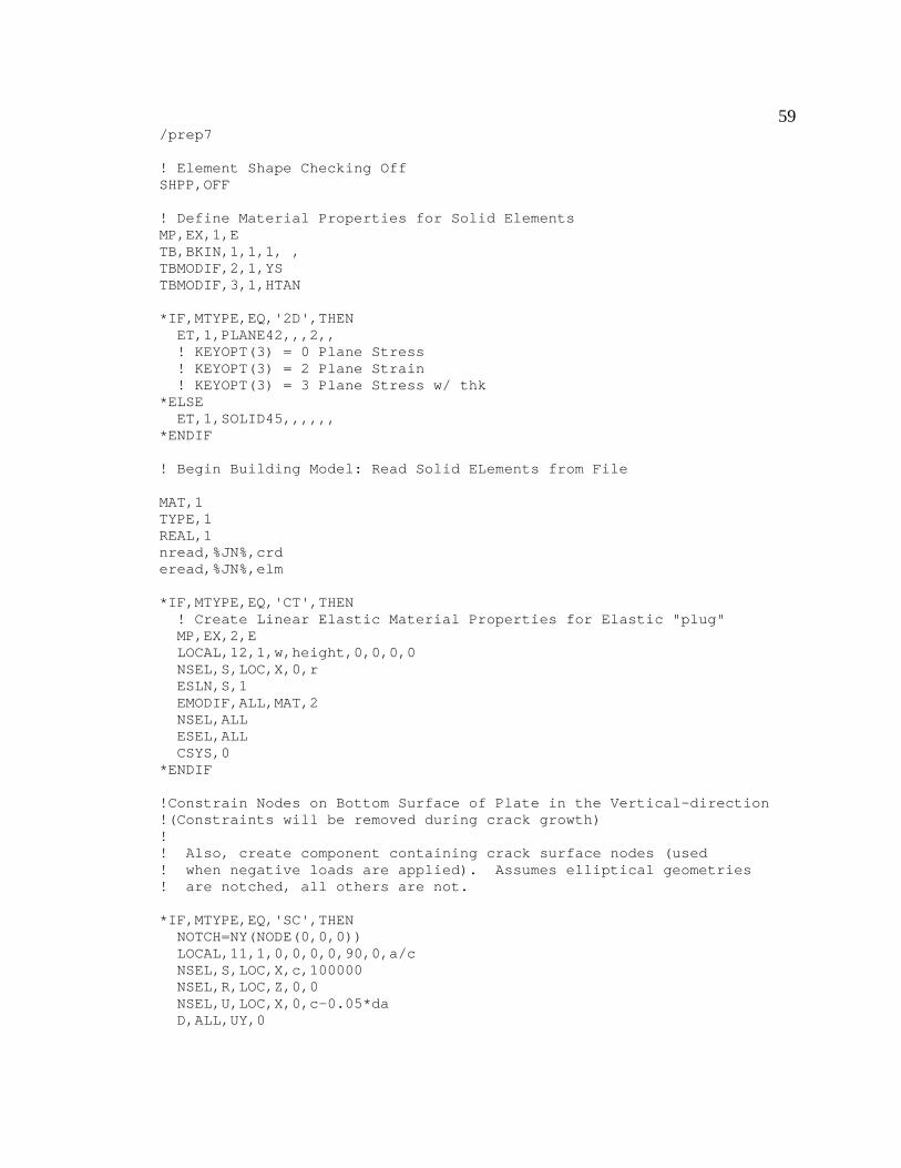
59 /prep7
! Element Shape Checking OffSHPP,OFF
! Define Material Properties for Solid ElementsMP,EX,1,ETB,BKIN,1,1,1, ,TBMODIF,2,1,YSTBMODIF,3,1,HTAN
*IF,MTYPE,EQ,'2D',THENET,1,PLANE42,,,2,,! KEYOPT(3) = 0 Plane Stress! KEYOPT(3) = 2 Plane Strain! KEYOPT(3) = 3 Plane Stress w/ thk
*ELSEET,1,SOLID45,,,,,,
*ENDIF
! Begin Building Model: Read Solid ELements from File
MAT,1TYPE,1REAL,1nread,%JN%,crderead,%JN%,elm
*IF,MTYPE,EQ,'CT',THEN! Create Linear Elastic Material Properties for Elastic "plug"MP,EX,2,ELOCAL,12,1,w,height,0,0,0,0NSEL,S,LOC,X,0,rESLN,S,1EMODIF,ALL,MAT,2NSEL,ALLESEL,ALLCSYS,0
*ENDIF
!Constrain Nodes on Bottom Surface of Plate in the Vertical-direction!(Constraints will be removed during crack growth)!! Also, create component containing crack surface nodes (used! when negative loads are applied). Assumes elliptical geometries! are notched, all others are not.
*IF,MTYPE,EQ,'SC',THENNOTCH=NY(NODE(0,0,0))LOCAL,11,1,0,0,0,0,90,0,a/cNSEL,S,LOC,X,c,100000NSEL,R,LOC,Z,0,0NSEL,U,LOC,X,0,c-0.05*daD,ALL,UY,0
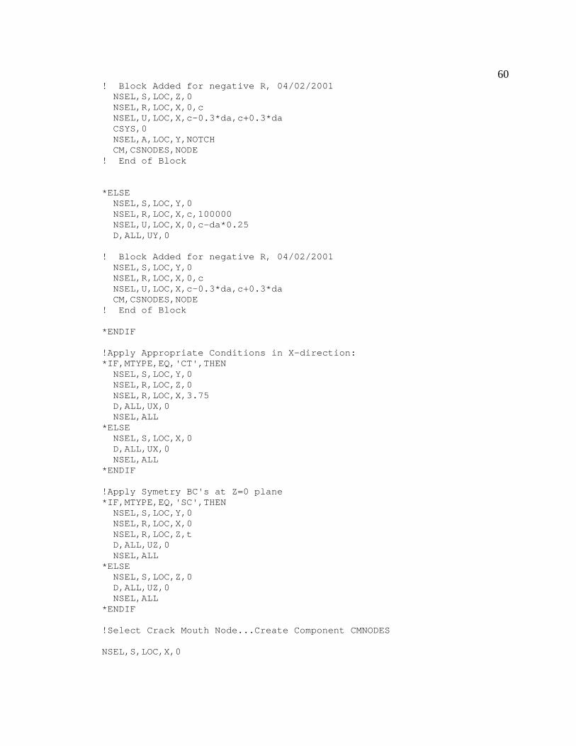
60
! Block Added for negative R, 04/02/2001NSEL,S,LOC,Z,0NSEL,R,LOC,X,0,cNSEL,U,LOC,X,c-0.3*da,c+0.3*daCSYS,0NSEL,A,LOC,Y,NOTCHCM,CSNODES,NODE
! End of Block
*ELSENSEL,S,LOC,Y,0NSEL,R,LOC,X,c,100000NSEL,U,LOC,X,0,c-da*0.25D,ALL,UY,0
! Block Added for negative R, 04/02/2001NSEL,S,LOC,Y,0NSEL,R,LOC,X,0,cNSEL,U,LOC,X,c-0.3*da,c+0.3*daCM,CSNODES,NODE
! End of Block
*ENDIF
!Apply Appropriate Conditions in X-direction:*IF,MTYPE,EQ,'CT',THEN
NSEL,S,LOC,Y,0NSEL,R,LOC,Z,0NSEL,R,LOC,X,3.75D,ALL,UX,0NSEL,ALL
*ELSENSEL,S,LOC,X,0D,ALL,UX,0NSEL,ALL
*ENDIF
!Apply Symetry BC's at Z=0 plane*IF,MTYPE,EQ,'SC',THEN
NSEL,S,LOC,Y,0NSEL,R,LOC,X,0NSEL,R,LOC,Z,tD,ALL,UZ,0NSEL,ALL
*ELSENSEL,S,LOC,Z,0D,ALL,UZ,0NSEL,ALL
*ENDIF
!Select Crack Mouth Node...Create Component CMNODES
NSEL,S,LOC,X,0

61
NSEL,R,LOC,Y,0CM,CMNODES,NODE
CMSEL,ALLNSEL,ALLESEL,ALL
WSORT,ALL,0 !Sort Elements to minimize wavefront
SAVEFINISH

62
APPENDIX A2
ANSYS INPUT FILE STRTCYC.MAC
CONTROL OF CYCLIC LOADING
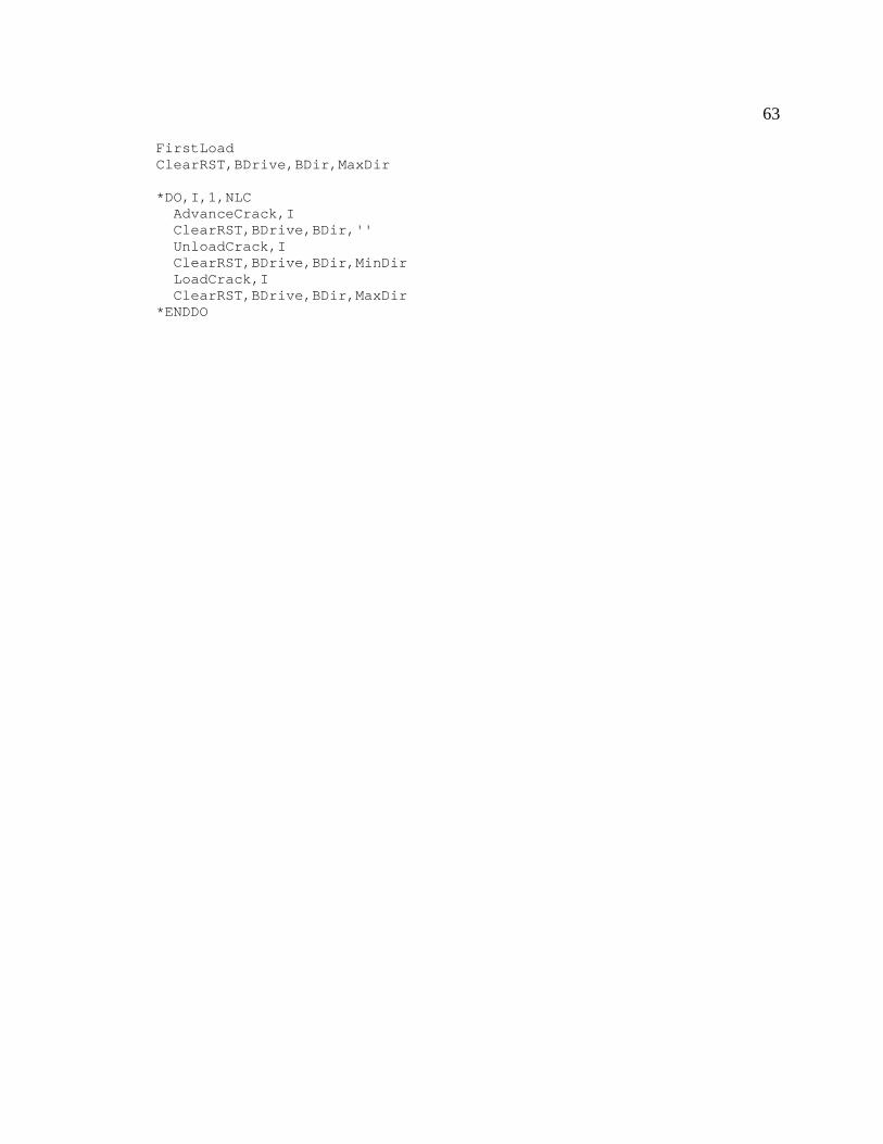
63
FirstLoadClearRST,BDrive,BDir,MaxDir
*DO,I,1,NLCAdvanceCrack,IClearRST,BDrive,BDir,''UnloadCrack,IClearRST,BDrive,BDir,MinDirLoadCrack,IClearRST,BDrive,BDir,MaxDir
*ENDDO

64
APPENDIX A3
ANSYS INPUT FILE FIRSTLOAD.MAC
APPLICATION OF FIRST LOAD

65 ! Apply Maximum Load on First Cycle:
! Calculate Elastic Limit:!/SOLU!AppLoad,height,1!AUTOTS,OFF!Solve!/POST1!NSORT,S,EQV,1,0!*GET,MaxStrs,SORT,,MAX!/SOLU!AppLoad,height,YS/MaxStrs!Time,(YS/MaxStrs)*0.45/(StrsMax)!SOLVE!SAVE!AppLoad,height,StrsMax!AUTOTS,ON!NSUBST,5,10000,5,ON!Time,0.45!SOLVE!SAVE
/SOLUAppload,height,StrsMaxAUTOTS,ONNSUBST,5,10000,5,ONTIME,0.45SOLVESAVE

66
APPENDIX A4
ANSYS INPUT FILE ADVANCECRACK.MAC
INCREMENTALLY ADVANCE THE CRACK TIP

67 ! AdvanceCrack.mac! Macro File to advance crack uniformly one element!! Should be executed as:!! AdvanceCrack,LoadCycleNumber!
AUTOTS,OFFNSUBST,1,1,1
/PREP7SelCTNodes,arg1*GET,NNODES,NODE,,COUNTNODNO=0*DO,JJ,1,NNODES
NODNO=NDNEXT(NODNO)*GET,NODERF,NODE,NODNO,RF,FYDDELE,NODNO,UYF,NODNO,FY,NODERF
*ENDDONSEL,ALLESEL,ALL/SOLUANTYPE,,REST
TimeVar=0.45+0.05/(NCGECut+1)+(arg1-1)Time,TimeVarSOLVESAVE
*DO,J,1,NCGECut-1/PREP7SelCTNodes,arg1NODNO=0*DO,JJ,1,NNODES
NODNO=NDNEXT(NODNO)*GET,NODERF,NODE,NODNO,F,FYF,NODNO,FY,NODERF/CGERF
*ENDDONSEL,ALLESEL,ALL/SOLUANTYPE,,RESTTimeVar=0.45+(J+1)*0.05/(NCGECut+1)+(arg1-1)Time,TimeVarSOLVESAVE
*ENDDO
/PREP7SelCTNodes,arg1NODNO=0*DO,JJ,1,NNODES
NODNO=NDNEXT(NODNO)

68
*GET,NODERF,NODE,NODNO,F,FYFDELE,NODNO,FY
*ENDDONSEL,ALLESEL,ALL/SOLUANTYPE,,RESTTimeVar=arg1-0.5Time,TimeVarSOLVESAVE

69
APPENDIX A5
ANSYS INPUT FILE UNLOADCRACK.MAC
UNLOAD MODEL

70 AUTOTS,ONNSUBST,1,100,1,OFF*CFOPEN,%JN%_unload_%arg1%,dat!*VWRITE! ("NODE# Node r NodeAng S/Smax UY OStat RemoteStress")CurrLInc=UIBCCStrsLvl=StrsMax/StrsMaxRStrs=StrsMax*DO,JJ,1,arg1
SelCTNodes,JJNSEL,U,D,UY,0*GET,NSNODES,NODE,,COUNT*IF,NSNODES,GT,0,THEN
NODNO=0*DO,JJJ,1,NSNODES
NODNO=NDNEXT(NODNO)NODYSTRS=UY(NODNO)*IF,MTYPE,EQ,'SC',THEN
CSYS,11NDANG=NY(NODNO)NXLOC=NX(NODNO)CSYS,0
*ELSENDANG=NZ(NODNO)NXLOC=NX(NODNO)
*ENDIFNodeStat=0*VWRITE,NODNO,NXLOC,NDANG,StrsLvl,NODYSTRS,NODESTAT,RSTRS
(F6.0,2X,E12.6,2X,E10.4,2X,F8.6,2X,E12.6,2X,F4.0,2X,E12.6)*ENDDO
*ENDIF*ENDDO
*DO,J,1,1/UIDCCTimeVar=TimeVar+CurrLInc*0.5RStrs=StrsMax-(StrsMax-StrsMin)*(TimeVar+0.5-arg1)/0.5*IF,TimeVar,GE,arg1,Then
RStrs=StrsMinTimeVar=arg1Time,TimeVarAppLoad,height,RStrsSOLVESAVE*EXIT
*ENDIFTime,TimeVarStrsLvl=RStrs/StrsMaxAppLoad,height,RStrsSOLVESAVEClearRST,BDrive,BDir,''OPENSTAT=0OpnRwCnt=0*DO,JJ,1,arg1

71
SelCTNodes,JJNSEL,U,D,UY,0*GET,NSNODES,NODE,,COUNT*IF,NSNODES,GT,0,THEN
NODNO=0*DO,JJJ,1,NSNODES
NodeStat=0NODNO=NDNEXT(NODNO)NODYSTRS=UY(NODNO)*IF,MTYPE,EQ,'SC',THEN
CSYS,11NDANG=NY(NODNO)NXLOC=NX(NODNO)CSYS,0
*ELSENDANG=NZ(NODNO)NXLOC=NX(NODNO)
*ENDIF*IF,NodYStrs*1e10,LT,0,THEN
CurrLInc=UIDCCOPENSTAT=1NODESTAT=1D,NODNO,UY,0
*ENDIF*VWRITE,NODNO,NXLOC,NDANG,StrsLvl,NODYSTRS,NodeStat,RStrs
(F6.0,2X,E12.6,2X,E10.4,2X,F8.6,2X,E12.6,2X,F4.0,2X,E12.6)*ENDDO
*ELSEIF,NSNODES,EQ,0,THENOpnRwCnt=OpnRwCnt+1
*ENDIF*ENDDONSEL,ALL
! Close Crack surface nodes if negative load applied! Added for negative R -- 04/02/2001
*IF,RStrs,LE,0,THENCMSEL,S,CSNODESNSEL,U,D,UY,0*GET,NSNODES,NODE,,COUNT*IF,NSNODES,GT,0,THEN
NODNO=0*DO,JJJ,1,NSNODES
NODNO=NDNEXT(NODNO)NODYSTRS=UY(NODNO)*IF,NodYStrs*1e10,LT,0,THEN
OPENSTAT=1D,NODNO,UY,0
*ENDIF*ENDDO
*ENDIF*ENDIF
! End of Block

72
*IF,OPENSTAT,EQ,1,THENTime,Timevar+CurrLInc*0.01SOLVESAVEClearRST,BDrive,BDir,''
*ENDIF*IF,OpnRwCnt,EQ,arg1,THEN
CurrLInc=UIACC*ENDIF
*ENDDO*CFCLOSE

73
APPENDIX A6
ANSYS INPUT FILE LOADCRACK.MAC
LOAD MODEL

74 AUTOTS,ONNSUBST,1,100,1,OFF*CFOPEN,%JN%_load_%arg1%,dat
!*VWRITE! ("NODE# Node r NodeAng S/Smax SY OStat RemoteStress")
CurrLInc=LIBCOStrsLvl=StrsMin/StrsMaxRStrs=StrsMin*DO,JJ,1,arg1
SelCTNodes,JJNSEL,R,D,UY,0*GET,NSNODES,NODE,,COUNT*IF,NSNODES,GT,0,THEN
NODNO=0*DO,JJJ,1,NSNODES
NODNO=NDNEXT(NODNO)*GET,NODYSTRS,NODE,NODNO,S,Y*IF,MTYPE,EQ,'SC',THEN
CSYS,11NDANG=NY(NODNO)NXLOC=NX(NODNO)CSYS,0
*ELSENDANG=NZ(NODNO)NXLOC=NX(NODNO)
*ENDIFNodeStat=0*VWRITE,NODNO,NXLOC,NDANG,StrsLvl,NODYSTRS,NODESTAT,RSTRS
(F6.0,2X,E12.6,2X,E10.4,2X,F8.6,2X,E12.6,2X,F4.0,2X,E12.6)*ENDDO
*ENDIF*ENDDO*DO,J,1,1/LIDCO
TimeVar=TimeVar+CurrLInc*0.45RStrs=(StrsMax-StrsMin)*(TimeVar-arg1)/0.45+StrsMin*IF,TimeVar,GE,arg1+0.45,Then
RStrs=StrsMaxTimeVar=arg1+0.45Time,TimeVarAppLoad,height,RStrsSOLVESAVE*EXIT
*ENDIFTime,TimeVarStrsLvl=RStrs/StrsMaxAppLoad,height,RStrsSOLVESAVEClearRST,BDrive,BDir,''OPENSTAT=0OpnRwCnt=0

75
*DO,JJ,1,arg1SelCTNodes,JJNSEL,R,D,UY,0*GET,NSNODES,NODE,,COUNT*IF,NSNODES,GT,0,THEN
NODNO=0*DO,JJJ,1,NSNODES
NodeStat=0NODNO=NDNEXT(NODNO)*GET,NodYStrs,NODE,NODNO,S,Y*IF,MTYPE,EQ,'SC',THEN
CSYS,11NDANG=NY(NODNO)NXLOC=NX(NODNO)CSYS,0
*ELSENDANG=NZ(NODNO)NXLOC=NX(NODNO)
*ENDIF*IF,NodYStrs*1e10,GT,0,THEN
CurrLInc=LIDCOOPENSTAT=1NODESTAT=1DDELE,NODNO,UY
*ENDIF*VWRITE,NODNO,NXLOC,NDANG,StrsLvl,NODYSTRS,NodeStat,RStrs
(F6.0,2X,E12.6,2X,E10.4,2X,F8.6,2X,E12.6,2X,F4.0,2X,E12.6)*ENDDO
*ELSEIF,NSNODES,EQ,0,THENOpnRwCnt=OpnRwCnt+1
*ENDIF*ENDDONSEL,ALL
! Block Added for negative R, 04/02/2001
CMSEL,S,CSNODESNSEL,R,D,UY,0*GET,NSNODES,NODE,,COUNT*IF,NSNODES,GT,0,THEN
NODNO=0*DO,JJJ,1,NSNODES
NODNO=NDNEXT(NODNO)*GET,NodYStrs,NODE,NODNO,S,Y*IF,NodYStrs*1e10,GT,0,THEN
OPENSTAT=1DDELE,NODNO,UY
*ENDIF*ENDDO
*ENDIF
! End of New Block
*IF,OPENSTAT,EQ,1,THEN

76
Time,Timevar+CurrLInc*0.01SOLVESAVEClearRST,BDrive,BDir,''
*ENDIF*IF,OpnRwCnt,EQ,arg1,THEN
CurrLInc=LIACO*ENDIF
*ENDDO*CFCLOSE

77
APPENDIX A7
ANSYS INPUT FILE APPLOAD.MAC
APPLY LOADING BOUNDARY CONDITIONS

78 ! This macro is used to apply Surface Pressure! along the top of the hole in the CT model!! The center of the hole should be at coordinates! x = w, y = h!! Use should be as follows:! SCappLoad,height,Pressure!! Created March 31,2000
*IF,MTYPE,EQ,'CT',THENNSEL,S,LOC,X,wNSEL,R,LOC,Y,arg1NSEL,R,LOC,Z,0F,ALL,FY,arg2NSEL,ALL
*ELSENSEL,S,LOC,Y,arg1
! D,ALL,UY,arg2SF,ALL,PRES,-arg2NSEL,ALL
*ENDIF

79
APPENDIX A8
ANSYS INPUT FILE CLEARRST.MAC
REMOVE UNNECESSARY FILES TO SAVE DISK SPACE

80 ! This Macro Saves Disk Space by deleting 'jobname'.rst! It also provides a tool for stopped jobs by saving the! db and rst from the last completed loadstep to a backup! directory! Execution of this macro should be done with the following command:! ClearRST,BDrive,Bdir1,Bdir2!! If Bdir2 is unneccessary, '' should be input!! Modified 1/28/2000
SAVEFINISH!pltpzone!/COPY,,RST,,,,%arg1%%arg2%%arg3%
/COPY,,EMAT,,,,%arg1%%arg2%%arg3%/COPY,,OSAV,,,,%arg1%%arg2%%arg3%/COPY,,ESAV,,,,%arg1%%arg2%%arg3%/COPY,,MNTR,,,,%arg1%%arg2%%arg3%/COPY,,DB,,,,%arg1%%arg2%%arg3%/DELETE,,RST/SOLUANTYPE,,REST

81
APPENDIX A9
ANSYS INPUT FILE SELCTNODES.MAC
SELECT THE CRACK-TIP NODES
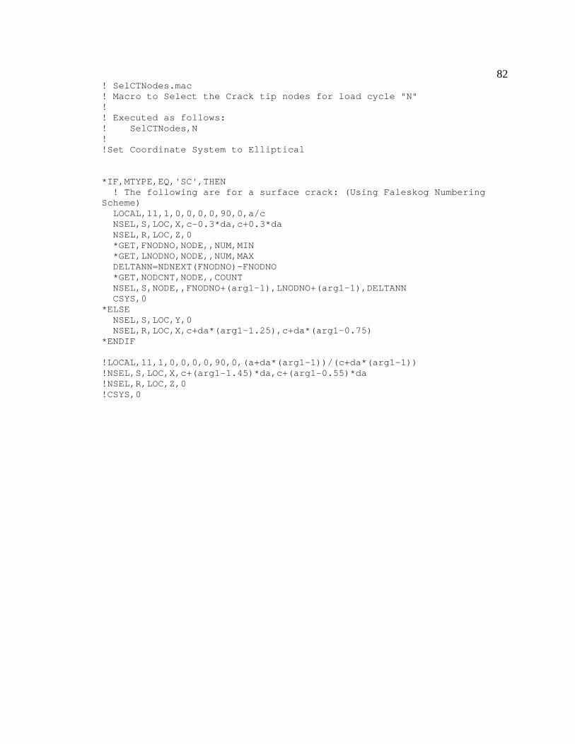
82 ! SelCTNodes.mac! Macro to Select the Crack tip nodes for load cycle "N"!! Executed as follows:! SelCTNodes,N!!Set Coordinate System to Elliptical
*IF,MTYPE,EQ,'SC',THEN! The following are for a surface crack: (Using Faleskog Numbering
Scheme)LOCAL,11,1,0,0,0,0,90,0,a/cNSEL,S,LOC,X,c-0.3*da,c+0.3*daNSEL,R,LOC,Z,0*GET,FNODNO,NODE,,NUM,MIN*GET,LNODNO,NODE,,NUM,MAXDELTANN=NDNEXT(FNODNO)-FNODNO*GET,NODCNT,NODE,,COUNTNSEL,S,NODE,,FNODNO+(arg1-1),LNODNO+(arg1-1),DELTANNCSYS,0
*ELSENSEL,S,LOC,Y,0NSEL,R,LOC,X,c+da*(arg1-1.25),c+da*(arg1-0.75)
*ENDIF
!LOCAL,11,1,0,0,0,0,90,0,(a+da*(arg1-1))/(c+da*(arg1-1))!NSEL,S,LOC,X,c+(arg1-1.45)*da,c+(arg1-0.55)*da!NSEL,R,LOC,Z,0!CSYS,0

83
APPENDIX B1
ANSYS INPUT FILE THROUGCRACK.DAT
3-D CENTER-CRACK GEOMETRY INPUT FILE

84 /batch! This is the input file for throughcrack.dat! This runs the script "appbcs.mac" to import the Solid! Elements and Nodes from the files "throughc.crd" & "throughc.elm",! and applies necessary boundary conditions for Crack Growth! It then calls "strtcyc.mac" to run growth analysis.
/CONFIG,NPROC,1
!Loading information:MTYPE='TC'
StrsMax=86.25e6StrsMin=8.625e6NLC=20
!Geometry Information:
t=0.00478 !Thickness of platew=0.04 !Plate Widthheight=0.08c=0.0196875 !Initial Crack half-lengtha=0da=0.3125e-4 !Crack Growth Increment
!Material Properties:
E=70e9 !Young's Modulus of specimenYS=345e6 !Yield Stress of Specimen
!Crack Growth Parameters
NCGECut=5CGERF=2
*get,JN,ACTIVE,,JOBNAM/TITLE, Plasticity Induced Closure of %JN%
AppBcs
BDrive='F:' ! Drive for file backupsBDir='\backup' ! Directory for file backupsMaxDir='\maxload' ! Directory for backup at Max LoadMinDir='\minload' ! Directory for Backup at Min Load
!Solution Information:
/SOLU ! Enter Solution Processor
LIBCO=0.05 ! Loading Increment before crack openingLIDCO=0.025 ! Loading Increment during crack openingLIACO=0.10 ! Loading Increment after crack openingUIBCC=0.05 ! Un-load Increment before crack closingUIDCC=0.025 ! Un-load Increment during crack closing

85
UIACC=0.10 ! Un-load Increment after crack closingSOLCONTROL,ONNSUB,1NEQIT,8 ! Number of Equillibrium Iterations beforebisectionNROPT,FULL,,ON ! Full Newton Rapson Option, Adaptive Descent ONEQSLV,PCG,1.0e-8 ! Use the Pre-Conditioned Conjugate Solver (InCore)
RESCONTROL,DEFINE,NONE,NONE,0 ! Set Resume Controls to act like! ANSYS 5.5.3 and below! (Single Frame Restart)
StrtCyc

86
APPENDIX B2
ANSYS INPUT FILE PCA0631.DAT
SAMPLE SURFACE CRACK INPUT FILE

87 /BATCH! This is the input file for pca1548! This runs the script "appbcs.mac" to import the Solid! Elements and Nodes from the files "jobname.crd" & "jobname.elm",! and applies necessary boundary conditions for Crack Growth! It then calls "strtcyc.mac" to run growth analysis.!! This script has been modified to work w/ ANSYS 5.6 and ANSYS 5.7! with the addition of the RESCONTROL Command (not valid for ANSYS 5.5and below)!! Modified 10/30/2000
!Note all lengths are in mm, and pressures in MPa
/CONFIG,NPROC,1
!Loading information:
StrsMax=150 ! Maximum Applied StressStrsMin=15 ! Minimum Applied StressNLC=10 ! Total Number of Loading Cycles to execute
!Geometry Information:
MTYPE='SC'
t=9.6 ! Thickness of platew=50.0 ! Plate Half-Widthheight=50.0 ! Model Heightc=9.547500 ! Initial Crack half-lengtha=2.998500 ! Initial Depth of Surface Crackda=0.00500 ! Crack Growth Increment
! Material Properties:
E=69.98e3 ! Young's ModulusYS=550.5 ! Yield Stress
! Crack Growth Options:
NCGECut=5 ! Number of bisections to matrix stiffnessbefore deathCGERF=2 ! Crack Growth Element Stiffness ReductionFactor
*get,JN,ACTIVE,,JOBNAM/TITLE, Plasticity Induced Closure of model %JN%
AppBCs ! Import Solid model and apply BC's
BDrive='E:' ! Drive for file backupsBDir='\backup' ! Directory for file backupsMaxDir='\maxload' ! Directory for backup at Max LoadMinDir='\minload' ! Directory for Backup at Min Load

88
!Solution Information:
/SOLU ! Enter Solution Processor
LIBCO=0.05 ! Loading Increment before crack openingLIDCO=0.025 ! Loading Increment during crack openingLIACO=0.10 ! Loading Increment after crack openingUIBCC=0.05 ! Un-load Increment before crack closingUIDCC=0.025 ! Un-load Increment during crack closingUIACC=0.10 ! Un-load Increment after crack closingSOLCONTROL,ONNSUB,1NEQIT,8 ! Number of Equillibrium Iterations beforebisectionNROPT,FULL,,ON ! Full Newton Rapson Option, Adaptive Descent ONEQSLV,PCG,1.0e-8 ! Use the Pre-Conditioned Conjugate Solver (InCore, default tolerance)
RESCONTROL,DEFINE,NONE,NONE,0 ! Set Resume Controls to act like! ANSYS 5.5.3 and below! (Single Frame Restart)
StrtCyc

89
APPENDIX C
CLOSURE ROUTINE USER’S GUIDE

90 CLOSUREGUIDE.TXT
USER’S GUIDE FOR THE PLASTICITY-INDUCED FATIGUE CRACKCLOSURE SCRIPTS WRITTEN BY JEFF SKINNER FOR USE WITH THEFINITE ELEMENT CODE ANSYS rev. 5.6
THE FOLLOWING ANSYS MACRO FILES MUST BE INCLUDED IN THEANSYS PATH. IF THE FILES ARE ALL LOCATED IN A COMMONDIRECTORY, THIS CAN BE ACCOMPLISHED BY SETTING THEANSYS_MACROLIB ENVIRONMENT VARIABLE IN THE OS).
ADVANCECRACK.MACAPPBCS.MACAPPLOAD.MACCLEARRST.MACFIRSTLOAD.MACLOADCRACK.MACSELCTNODES.MACSTRTCYC.MACUNLOADCRACK.MAC
THE FOLLOWING FILES MUST BE LOCATED IN THE ANSYS WORKINGDIRECTORY:
JOBNAME.CRDJOBNAME.ELMJOBNAME.DAT
WHERE,
JOBNAME IS THE EIGHT LETTER JOBNAME FOR THE ANSYS RUN
JOBNAME.CRD CONTAINS THE NODAL COORDINATES FOR THE MESHJOBNAME.ELM CONTAINS THE ELEMENT CONNECTIVITY FOR THE MESH
THESE MESH FILES CAN BE GENERATED FROM AN EXISTINGANSYS MESH USING “NWRITE,JOBNAME,CRD” AND“EWRITE,JOBNAME,ELM”.
JOBNAME.DAT ANSYS INPUT FILE WHICH CONTAINS THE MODELGEOMETRY AND LOADING INFORMATION AND ALSOCALLS THE ANSYS MACROS LISTED ABOVE.
THIS FILE SHOULD BE USED AS THE INPUT FILE FORRUNNING THE SCRIPTS IN BATCH MODE.

91
IN READING THIS GUIDE, LINES STARTING WITH “>” ARE LINESTHAT ARE COMMANDS, WORDS IN ITALICS SHOULD NOT BE TYPED.
THE INPUT FILE JOBNAME.DAT MUST CONTAIN THE FOLLOWING:1. A LINE CONTAINING THE MODEL TYPE:
>MTYPE=CODE
WHERE CODE = ‘SC’ FOR SURFACE CRACKED GEOMETRIES‘TC’ FOR 3-D CENTER CRACKED GEOMETRIES‘2D’ FOR 2-D CENTER CRACKED GEOMETRIES‘CT’ FOR 3-D COMPACT TENSION GEOMETRY
2. THE MAXIMUM AND MINIMUM APPLIED LOAD:
>StrsMax=MaxLoad>StrsMin=MinLoad
WHERE MaxLoad = MAXIMUM APPLIED FORCE FOR COMPACT TENSIONOR MAX. SURFACE TRACTION (OTHER GEOMETRIES)
MinLoad = MINIMUM APPLIED FORCE FOR COMPACT TENSIONOR MIN. SURFACE TRACTION (OTHER GEOMETRIES)
3. NUMBER OF LOAD CYCLES:
>NLC = I
4. GEOMETRY INFORMATION:
>T= Model Thickness (Z-Direction)>W= Model Width (X-Direction)>HEIGHT= Model Height (Y-Direction)>C= Crack Length (From Origin to Crack Tip in X-Direction)>A= Crack Depth (From Origin to Crack Tip in Z-Direction)>DA= Crack Growth Increment (Constant along Crack Front)
5. MATERIAL PROPERTIES (BI-LINEAR KINEMATIC MATERIAL):
>E = Elastic Modulus>YS = Yield Stress>HTAN = Tangent Modulus
6. CRACK GROWTH PARAMETERS:

92
>NCGECUT = Number of Cuts to Nodal Reaction Force duringCrack Advance
>CGERF = Factor to Reduce Nodal Reaction Force duringAdvance (NodeForce = NodeForce / CGERF)
7. A LINE TO GET THE ACTIVE JOBNAME:
>*GET,JN,ACTIVE,,JOBNAM
8. A CALL TO THE SCRIPT TO APPLY THE BOUNDARY CONDITIONS:
>AppBcs
THIS SCRIPT ASSUMES MODELS ARE ORIENTED WITH THE CRACKGROWING IN THE GLOBAL X-DIRECTION (THROUGHCRACKS) OR IN THEX AND Z DIRECTIONS (SURFACE CRACKS), WITH THE Y=0 PLANE ASTHE CRACK PLANE (PLANE OF SYMMETRY). ALSO, OTHER PLANES OFSYMMETRY SHOULD BE LOCATED ON THE X=0 AND Z=0 PLANES THREEPLANES OF SYMMETRY EXIST.
9. DIRECTORY INFORMATION FOR BACKUPS:
>BDRIVE = Drive Letter>BDIR = Directory Name for Back-up after every Load-Step>MaxDir = Directory Name for Back-up at Max Load>MinDir = Directory Name for Back-up at Min Load
THE SCRIPT CLEARST WILL USE THESE DIRECTORIES TO BACK-UPTHE NECESSARY RESTART INFORMATION. ALSO, THE MaxDir andMinDir PROVIDE A CONVIENENT WAY TO POST-PROCESS AT MAXIMUMAND MINIMUM LOAD.
10. SOLUTION INFORMATION:
ENTER THE SOLUTION PROCESSOR:
>/SOLU
LOAD INCREMENTS-Defined as Percentage of Range(Smax-Smin):
>LIBCO= Load Increment Before Any Node Opens>LIDCO= Load Increment During Crack Opening>LIACO= Load Increment After Crack is Fully Open>UIBCC= Un-Load Increment Before Any Node Closes>UIDCC= Un-Load Increment During Crack Closing

93
>UIACC= Un-Load Increment After Crack is Closed
NONLINEAR CONTROLS:
>SOLCONTROL,ON>NSUB,1>NEQIT,8FULL NEWTON-RHAPSON METHOD WITH ADAPIVE DECENT:
>NROPT,FULL,ON
USE THE PRE-CONDITIONED CONJUGATE GRADIENT SOLVER WITHLOOSER TOLERANCE – Necessary only if large model (more than50,000 degrees of freedom):
>EQSLV,PCG,1.0e-4
RESUME CONTOL – Must be used for Ansys 5.6 or greater.
>RESCONTROL,DEFINE,NONE,NONE,0
11. CALL TO START REMAINING CYCLE:
>StrtCyc

94
APPENDIX D
FORTRAN PROGRAM ANSMESH54.FOR
CONVERTS SCPCELL.EXE MESH FILES TO ANSYS
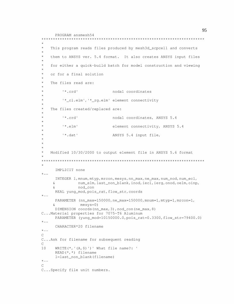
95 PROGRAM ansmesh54
************************************************************************* This program reads files produced by mesh3d_scpcell and converts** them to ANSYS ver. 5.4 format. It also creates ANSYS input files** for either a quick-build batch for model construction and viewing** or for a final solution** The files read are:** '*.crd' nodal coordinates** '*_cl.elm','*_rg.elm' element connectivity** The files created/replaced are:** '*.crd' nodal coordinates, ANSYS 5.4** '*.elm' element connectivity, ANSYS 5.4** '*.dat' ANSYS 5.4 input file,**** Modified 10/30/2000 to output element file in ANSYS 5.6 format*************************************************************************
IMPLICIT none*--
INTEGER l,mnum,mtyp,mrcon,mesys,nn_max,ne_max,num_nod,num_ecl,& num_elm,last_non_blank,inod,iecl,ierg,onod,oelm,oinp,& nod_conREAL yung_mod,pois_rat,flow_str,coords
*--PARAMETER (nn_max=150000,ne_max=150000,mnum=1,mtyp=1,mrcon=1,
& mesys=0)DIMENSION coords(nn_max,3),nod_con(ne_max,8)
C...Material properties for 7075-T6 AluminumPARAMETER (yung_mod=10150000.0,pois_rat=0.3300,flow_str=79400.0)
*--CHARACTER*20 filename
*--CC...Ask for filename for subsequent readingC10 WRITE(*,'(A,$)')' What file name?: '
READ(*,*) filenamel=last_non_blank(filename)
*--CC...Specify file unit numbers.
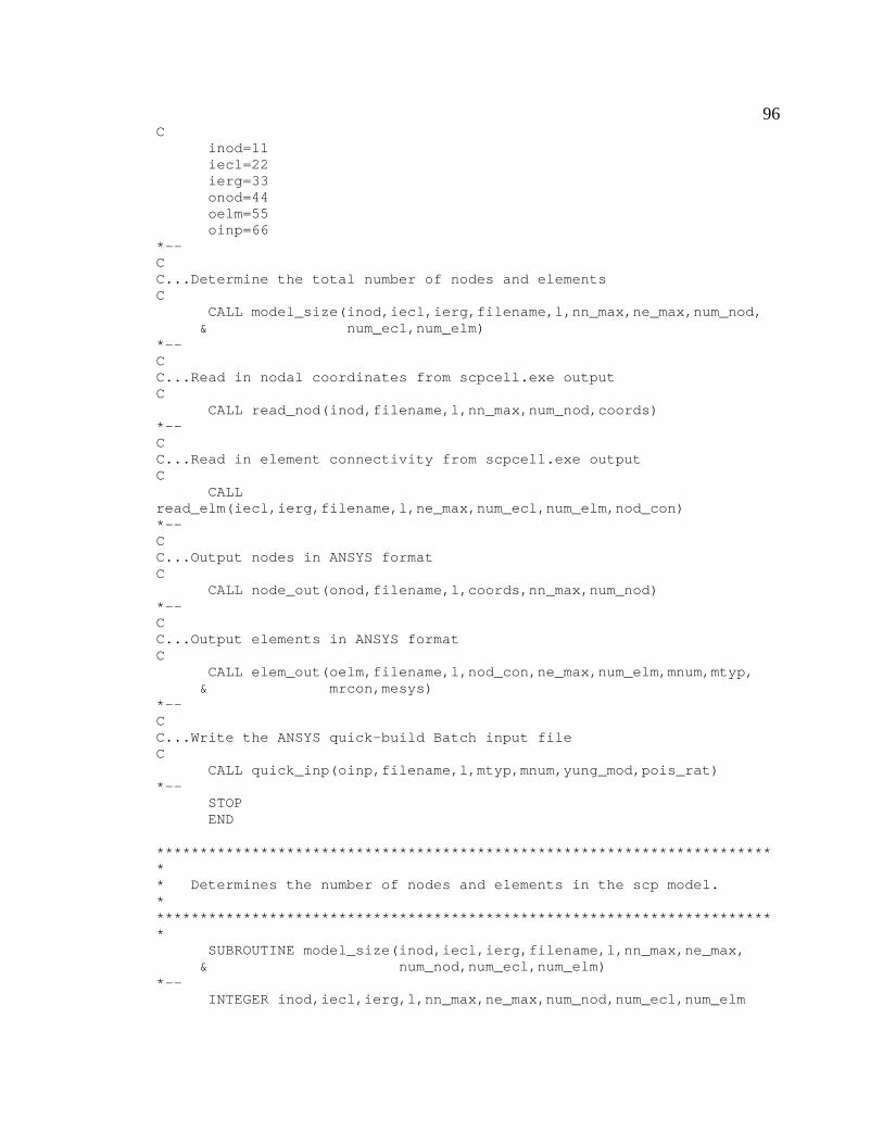
96C
inod=11iecl=22ierg=33onod=44oelm=55oinp=66
*--CC...Determine the total number of nodes and elementsC
CALL model_size(inod,iecl,ierg,filename,l,nn_max,ne_max,num_nod,& num_ecl,num_elm)
*--CC...Read in nodal coordinates from scpcell.exe outputC
CALL read_nod(inod,filename,l,nn_max,num_nod,coords)*--CC...Read in element connectivity from scpcell.exe outputC
CALLread_elm(iecl,ierg,filename,l,ne_max,num_ecl,num_elm,nod_con)*--CC...Output nodes in ANSYS formatC
CALL node_out(onod,filename,l,coords,nn_max,num_nod)*--CC...Output elements in ANSYS formatC
CALL elem_out(oelm,filename,l,nod_con,ne_max,num_elm,mnum,mtyp,& mrcon,mesys)
*--CC...Write the ANSYS quick-build Batch input fileC
CALL quick_inp(oinp,filename,l,mtyp,mnum,yung_mod,pois_rat)*--
STOPEND
************************************************************************* Determines the number of nodes and elements in the scp model.*************************************************************************
SUBROUTINE model_size(inod,iecl,ierg,filename,l,nn_max,ne_max,& num_nod,num_ecl,num_elm)
*--INTEGER inod,iecl,ierg,l,nn_max,ne_max,num_nod,num_ecl,num_elm
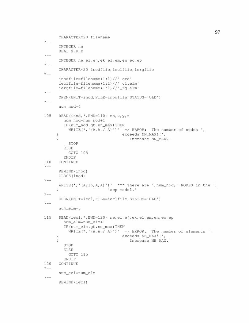
97CHARACTER*20 filename
*--INTEGER nnREAL x,y,z
*--INTEGER ne,ei,ej,ek,el,em,en,eo,ep
*--CHARACTER*20 inodfile,ieclfile,iergfile
*--inodfile=filename(1:l)//'.crd'ieclfile=filename(1:l)//'_cl.elm'iergfile=filename(1:l)//'_rg.elm'
*--OPEN(UNIT=inod,FILE=inodfile,STATUS='OLD')
*--num_nod=0
105 READ(inod,*,END=110) nn,x,y,znum_nod=num_nod+1IF(num_nod.gt.nn_max)THEN
WRITE(*,'(A,A,/,A)')' => ERROR: The number of nodes ',& 'exceeds NN_MAX!!',& ' Increase NN_MAX.'
STOPELSE
GOTO 105ENDIF
110 CONTINUE*--
REWIND(inod)CLOSE(inod)
*--WRITE(*,'(A,I6,A,A)')' *** There are ',num_nod,' NODES in the ',
& 'scp model.'*--
OPEN(UNIT=iecl,FILE=ieclfile,STATUS='OLD')*--
num_elm=0
115 READ(iecl,*,END=120) ne,ei,ej,ek,el,em,en,eo,epnum_elm=num_elm+1IF(num_elm.gt.ne_max)THEN
WRITE(*,'(A,A,/,A)')' => ERROR: The number of elements ',& 'exceeds NE_MAX!!',& ' Increase NE_MAX.'
STOPELSE
GOTO 115ENDIF
120 CONTINUE*--
num_ecl=num_elm*--
REWIND(iecl)
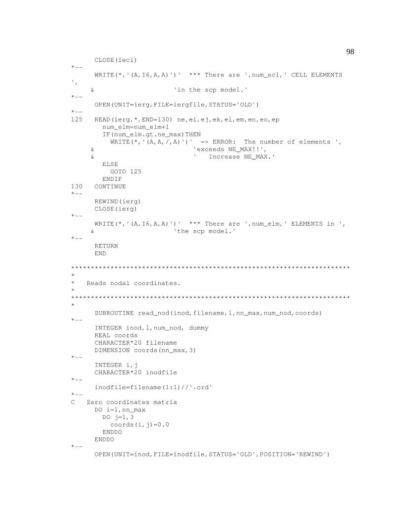
98CLOSE(iecl)
*--WRITE(*,'(A,I6,A,A)')' *** There are ',num_ecl,' CELL ELEMENTS
',& 'in the scp model.'
*--OPEN(UNIT=ierg,FILE=iergfile,STATUS='OLD')
*--125 READ(ierg,*,END=130) ne,ei,ej,ek,el,em,en,eo,ep
num_elm=num_elm+1IF(num_elm.gt.ne_max)THEN
WRITE(*,'(A,A,/,A)')' => ERROR: The number of elements ',& 'exceeds NE_MAX!!',& ' Increase NE_MAX.'
ELSEGOTO 125
ENDIF130 CONTINUE*--
REWIND(ierg)CLOSE(ierg)
*--WRITE(*,'(A,I6,A,A)')' *** There are ',num_elm,' ELEMENTS in ',
& 'the scp model.'*--
RETURNEND
************************************************************************* Reads nodal coordinates.*************************************************************************
SUBROUTINE read_nod(inod,filename,l,nn_max,num_nod,coords)*--
INTEGER inod,l,num_nod, dummyREAL coordsCHARACTER*20 filenameDIMENSION coords(nn_max,3)
*--INTEGER i,jCHARACTER*20 inodfile
*--inodfile=filename(1:l)//'.crd'
*--C Zero coordinates matrix
DO i=1,nn_maxDO j=1,3
coords(i,j)=0.0ENDDO
ENDDO*--
OPEN(UNIT=inod,FILE=inodfile,STATUS='OLD',POSITION='REWIND')

99*--
WRITE(*,'(A,A)')' *** Reading nodal coordinates from file: ',& inodfile
*--C Read nodal coordinates from scpcell.exe output
DO i=1,num_nodREAD(inod,*) dummy,(coords(i,j),j=1,3)
ENDDO*--
CLOSE(inod)*--
WRITE(*,'(A,I6,A,13X,A)')' ***',num_nod,' NODES read fromfile:',
& inodfile*--
RETURNEND
************************************************************************* Returns the position of the last non-blank character in thestring.** Returns zero if string is all blanks.*************************************************************************
INTEGER FUNCTION last_non_blank(string)IMPLICIT NONECHARACTER string*(*)INTEGER i,i2
*--i=LEN(string)i2=0DO WHILE (i.GT.i2)
IF(string(i:i).NE.' ') i2=ii=i-1
ENDDOlast_non_blank=i2
*--RETURNEND
************************************************************************* Reading element connectivity files.*************************************************************************
SUBROUTINE read_elm(iecl,ierg,filename,l,ne_max,num_ecl,num_elm,& nod_con)
*--INTEGER iecl,ierg,l,nod_con,ne_max,num_ecl,num_elm, dummyCHARACTER*20 filename

100DIMENSION nod_con(ne_max,8)
*--INTEGER i,jCHARACTER*20 ieclfile,iergfile
*--ieclfile=filename(1:l)//'_cl.elm'iergfile=filename(1:l)//'_rg.elm'
*--C Zero connectivity matrix
DO i=1,ne_maxDO j=1,8
nod_con(i,j)=0ENDDO
ENDDO*--
OPEN(UNIT=iecl,FILE=ieclfile,STATUS='OLD')*--
WRITE(*,'(A,A)')' *** Reading element connectivity from file: ',& ieclfile
*--C Read element connectivity from *_cl.elm file
DO i=1,num_eclREAD(iecl,*) dummy,(nod_con(i,j),j=1,8)
ENDDO*--
WRITE(*,260) num_ecl,ieclfile*--
CLOSE(iecl)*--
OPEN(UNIT=ierg,FILE=iergfile,STATUS='OLD')*--
WRITE(*,'(A,A)')' *** Reading element connectivity from file: ',& iergfile
*--C Read element connectivity from *_rg.elm file
DO i=num_ecl+1,num_elmREAD(ierg,*) dummy,(nod_con(i,j),j=1,8)
ENDDO*--
WRITE(*,260) num_elm,iergfile*--
CLOSE(ierg)*--260 FORMAT(' ***',I6,' ELEMENTS read from file:',10X,A20)*--
RETURNEND
************************************************************************* Output nodal coordinates in ANSYS format.*

101************************************************************************
SUBROUTINE node_out(onod,filename,l,coords,nn_max,num_nod)*--
INTEGER onod,l,nn_max,num_nodREAL coordsCHARACTER*20 filenameDIMENSION coords(nn_max,3)
*--INTEGER i,jREAL THCHARACTER*20 onodfile
*--onodfile=filename(1:l)//'.crd'
*--th=0.0
*--OPEN(UNIT=onod,FILE=onodfile,STATUS='REPLACE',POSITION='REWIND')
*--DO i=1,num_nod
WRITE(onod,355) i,(coords(i,j),j=1,3),th,th,thENDDO
*--CLOSE(onod)
*--WRITE(*,'(A,I6,A,12X,A)')' ***',num_nod,' NODES written to
file:'& ,onodfile
*--355 FORMAT(I8,6G20.13)*--
RETURNEND
************************************************************************* Output element connectivity in ANSYS format.*************************************************************************
SUBROUTINE elem_out(oelm,filename,l,nod_con,ne_max,num_elm,mnum,& mtyp,mrcon,mesys)
*--INTEGER oelm,l,nod_con,ne_max,num_elm,mnum,mtyp,mrcon,mesysCHARACTER*20 filenameDIMENSION nod_con(ne_max,8)
*--INTEGER i,jCHARACTER*20 oelmfile
*--oelmfile=filename(1:l)//'.elm'
*--OPEN(UNIT=oelm,FILE=oelmfile,STATUS='UNKNOWN')
*--

102DO i=1,num_elm
WRITE(oelm,455) (nod_con(i,j),j=1,8),mnum,mtyp,mrcon,1,mesys,iENDDO
*--CLOSE(oelm)
*--WRITE(*,'(A,I6,A,A,9X,A)')' ***',num_elm,' ELEMENTS written to '
& ,'file:',oelmfile*--455 FORMAT(14I6,2X)*--
RETURNEND
************************************************************************* Build ANSYS input file for QUICK batch build.*************************************************************************
SUBROUTINE quick_inp(oinp,filename,l,mtyp,mnum,yung_mod,pois_rat)*--
INTEGER oinp,l,mnumCHARACTER*20 filename,oinpfile,nodefile,elemfileREAL yung_mod,pois_rat
*--oinpfile=filename(1:l)//'.dat'nodefile=filename(1:l)//',crd'elemfile=filename(1:l)//',elm'
*--OPEN(UNIT=oinp,FILE=oinpfile,STATUS='UNKNOWN')
*--* WRITE(oinp,'(A)')'/batch'
WRITE(oinp,20)20 FORMAT('C*** This file was generated by "ansmesh54.exe" forthe',
& 'C*** sole purpose of creating models quickly using Batchmode'
&,'C*** in model construction')WRITE(oinp,'(/,A)')'/prep7'WRITE(oinp,'(A)')'/nerr,5,60000'WRITE(oinp,'(A,23X,A)')'shpp,off'
* & '!turn off element shape checking'WRITE(oinp,'(A,I1,A)')'et,',mtyp,',SOLID45,,,,1'WRITE(oinp,'(A,I1,A,F9.0)')'mp,ex,',mnum,',',yung_modWRITE(oinp,'(A,I1,A,F9.0)')'mp,ey,',mnum,',',yung_modWRITE(oinp,'(A,I1,A,F9.0)')'mp,ez,',mnum,',',yung_modWRITE(oinp,'(A,I1,A,F6.4)')'mp,nuxy,',mnum,',',pois_ratWRITE(oinp,'(A,I1,A,F6.4)')'mp,nuyz,',mnum,',',pois_ratWRITE(oinp,'(A,I1,A,F6.4)')'mp,nuxz,',mnum,',',pois_ratWRITE(oinp,'(A,A)')'nread,',nodefileWRITE(oinp,'(A,A)')'eread,',elemfile
* WRITE(oinp,'(A)')'finish'* WRITE(oinp,'(A)')'/exit'

103*--
CLOSE(oinp)*--
WRITE(*,'(A,A,A)')' ***ANSYS input for quick-build option ',& 'written to file: ',oinpfile
*--RETURNEND

104
APPENDIX E
INPUT FILE MESH3D_SCPCELL.IN
MESH GENERATION INPUT FILE

105 FILE: mesh3d_scpcell.in===== In-put-data for the mesh-generating program mesh3d_scpcell.f
NAMEPROGRAM (ABAQUS WARP3D or PATRAN)DATE (ex. sept. 30, 1996 960930 Europe; 093096 USA)ncell D eta_n necbeta_tI eta_tII ncdI ncdIIp_lcx1 p_lcx2 p_alfacmr sfred sfred_type mv sjred_typem1 m2mb nb mbtype mb_biaslt lred rtypeetypt w c aY0 Z10 Z20Y1 Z11 Z21Y2 Z12 Z22- - - - -- - - - -- - - - -Ynla Z1nla Z2nla
*INDATApca0631PATRAN000106ncell=40 D=0.01000 eta_n=0.5 necb=3eta_tI=2.5 eta_tII=18.0 ncdI=4 ncdII=4p_lcxI=1.6 p_lcxII=2.8 p_alfac=0.45mr=8 sfred=4 sfred_type=2 mv=3 sjred_type=3m_I=20 m_II=10mb=4 nb=10 mbtype=0 mb_bias=1.10lt=13 lred=7 rtype=2etyp=8
t=4.7616 w=22.2500 c=9.52500 a=2.976000.0000 0 4.76160.0750 0 4.76160.1500 0 4.76160.2250 0 4.76160.5000 0 4.76161.6830 0 4.76162.3250 0 4.76163.1360 0 4.76164.1610 0 4.76169.4700 0 4.7616
16.2450 0 4.761624.8900 0 4.761635.9220 0 4.761650.0000 0 4.7616

106
APPENDIX F
FORTRAN PROGRAM CLOSINTERP.F90
INTERPOLATION OF OPENING LEVELS

107
! ClosInterp.f90 ----------------------------------------------------!! Program to read the output from the ANSYS closure macros! and do a linear interpolation to determine the closing/opening! stress for the nodes behind the crack-tip!! -------------------------------------------------------------------
CHARACTER(28) :: InFile, OutFile, JobNameCHARACTER(2) :: CycleNoINTEGER :: J, NLC
WRITE (*,'(1X,A)', ADVANCE="NO") "Enter Ansys JobName:"READ *, JobNameWRITE (*,'(1X,A)', ADVANCE="NO") "Enter Number of Loading CyclesCompleted: "READ *, NLC
WRITE(*,*) JobName
DO J=1,NLCCALL INT2STR(J,CycleNo)
InFile=JobName(1:LEN_TRIM(JobName))//'_load_'//CycleNo(1:LEN_TRIM(CycleNo))//'.dat'
OutFile='L'//CycleNo(1:LEN_TRIM(CycleNo))//'.txt'WRITE(*,*) InFile,OutFileCALL Interp(InFile,OutFile)
InFile=JobName(1:LEN_TRIM(JobName))//'_unload_'//CycleNo(1:LEN_TRIM(CycleNo))//'.dat'
OutFile='UL'//CycleNo(1:LEN_TRIM(CycleNo))//'.txt'WRITE(*,*) InFile,OutFileCALL Interp(InFile,OutFile)
ENDDO
CONTAINS
SubRoutine Interp(InFile,OutFile)
CHARACTER(28), INTENT(IN) :: InFile, OutFileINTEGER :: OpenStatus, InputStatus, Count, M, NREAL::Nodno,NX,NdAng,StrsLvl,NodYStrs,NodStat,CNodno,NodYStrs0,StrsLvl0
OPEN(UNIT=10, FILE=InFile, STATUS="OLD", IOSTAT = OpenStatus)IF (OpenStatus > 0) STOP "**** Cannot Open File ****"
OPEN(UNIT=20, FILE=OutFile, STATUS="REPLACE", IOSTAT = OpenStatus)IF (OpenStatus > 0) STOP "**** Cannot Open File ****"
100 FORMAT(E12.6,E12.6,F8.4,E14.6)
! Determine the number of lines before repeatingCount = 0

108CALL ReadLine(CNodno,NX,NdAng,StrsLvl,NodYStrs,InputStatus,NodStat)DO
Count=Count+1CALL ReadLine(Nodno,NX,NdAng,StrsLvl,NodYStrs,InputStatus,NodStat)IF (InputStatus < 0) EXIT !End of FileIF(Nodno==CNodno) EXIT
ENDDO
WRITE (*,*) COUNT
DO M=1, COUNTREWIND 10
DO N=1, MCALL
ReadLine(CNodno,NX,NdAng,StrsLvl0,NodYStrs0,InputStatus,NodStat)IF (InputStatus < 0) EXIT !End of File
ENDDO
IF (NodStat == 1) THENWRITE (UNIT=20,FMT=100) NdAng, NX, StrsLvl0, NodYStrs0CYCLE
ENDIF
DOCALL ReadLine(Nodno,NX,NdAng,StrsLvl,NodYStrs,InputStatus,NodStat)IF (InputStatus < 0) EXIT !End of FileIF (Nodno==CNodno) THEN
IF (NodStat == 1) THEN!InterpolateStrsLvl=(NodYStrs*StrsLvl0-NodYStrs0*StrsLvl)/(NodYStrs-NodYStrs0)WRITE (UNIT=20,FMT=100) NdAng, NX, StrsLvl, NodYStrs
EXITELSE
StrsLvl0 = StrsLvlNodYStrs0 = NodYStrs
END IFEND IF
ENDDOENDDOCLOSE(10)CLOSE(20)
END SubRoutine Interp
SubRoutineReadLine(Nodno,NX,NdAng,StrsLvl,NodYStrs,InputStatus,NodeStat)
REAL, INTENT(OUT)::Nodno,NX,NdAng,StrsLvl,NodYStrs,NodeStatREAL::RStrsINTEGER, INTENT(OUT)::InputStatusREAD (10,*, IOSTAT=InputStatus) NodNo, NX, NdAng, StrsLvl, &
NodYStrs, NodeStat, RStrsIF (InputStatus > 0) STOP "**** Input Error ****"

109END SubRoutine ReadLine
SubRoutine INT2STR(InINT,OutStr)! This Subroutine Converts a 2 digit Integer (0 - 99) to a Characterof Dimension 2
INTEGER, INTENT(IN):: InINTCHARACTER(2), INTENT(OUT)::OutStrCHARACTER(1):: C1,C2
IF (InINT.GE.10) THENC1=CHAR(InINT/10 +48)C2=CHAR(InINT-(InINT/10)*10+48)OutStr=C1//C2WRITE(*,*) OutStr
ELSEC1=CHAR(InINT+48)OutStr=C1WRITE(*,*) OutStr
END IF
END SubRoutine INT2STR
END