CODEE Journal

Volume 11 Article 1

12-29-2018

Find, Process, and Share: An Optimal Control inthe Vidale-Wolfe Marketing ModelMichael C. BargNiagara University, mbarg@niagara.edu

Follow this and additional works at: https://scholarship.claremont.edu/codee

Part of the Economics Commons, Marketing Commons, Mathematics Commons, and theScience and Mathematics Education Commons

This Article is brought to you for free and open access by the Journals at Claremont at Scholarship @ Claremont. It has been accepted for inclusion inCODEE Journal by an authorized editor of Scholarship @ Claremont. For more information, please contact scholarship@cuc.claremont.edu.

Recommended CitationBarg, Michael C. (2016) "Find, Process, and Share: An Optimal Control in the Vidale-Wolfe Marketing Model," CODEE Journal: Vol.11, Article 1.Available at: https://scholarship.claremont.edu/codee/vol11/iss2/1

Find, Process, and Share: An Optimal Control in the Vidale-WolfeMarketing Model

Cover Page Footnote (optional)The author thanks Beverly West and Brian Winkel for their encouragement to produce this article afterhearing our talk on the subject at the MAA Contributed Paper Session: The Teaching and Learning ofUndergraduate Ordinary Differential Equations during the 2017 Joint Mathematics Meetings.

This article is available in CODEE Journal: https://scholarship.claremont.edu/codee/vol11/iss2/1

Find, Process, and Share: An Optimal Control in theVidale-Wolfe Marketing Model

Michael C. BargNiagara University

Keywords: Vidale-Wolfe marketing model, ODE reading project, optimal control, Green’stheoremManuscript received on January 18, 2018; published on December 29, 2018.

Abstract: The Vidale-Wolfe marketing model is a first-order, linear, non-homogeneous ordinary differential equation (ODE) where the forcing term isproportional to advertising expenditure. With an initial response in sales asthe initial condition, the solution of the initial value problem is straightfor-ward for a first undergraduate ODE course. The model serves as an excellentexample of many relevant topics for those students whose interests lie ineconomics, finance, or marketing. Its inclusion in the curriculum is partic-ularly rewarding at an institution without a physics program. The modelis not new, but it was novel to us when a group of students chose it for anexploratory project that we designed in order to help students acquire theability to interpret and communicate mathematical results. In addition todescribing the project in this work, we discuss the Vidale-Wolfe model andshow how it can lead one to use Green’s theorem in a real situation.

1 Introduction

As mathematicians and educators in higher education, we are steeped in a find, process,and share mentality. Indeed, we spend hours scouring the literature for research related toour own. We process what we have found and synthesize new directions. After muchwork,we share our results with the community through papers and presentations. If educationis our focus, we perform similar steps: finding and learning about new pedagogicaldevelopments; processing to determine what will work within our classroom and teachingmode or style; and, ultimately, sharing our work with students, fellow educators, and thelarger academic community through classes, discussion at workshops, and by other means.In this article, we are excited to report on our finding of the Vidale-Wolfe marketing model.Our process has shed light on some great mathematics that can be gleaned from a carefulanalysis of the model. We share our story with the hope that other educators might findthe model appropriate for processing and sharing with their own students.

We begin in Section 2 with details about an ordinary differential equations (ODEs)reading and writing course project. Section 3 presents the Vidale-Wolfe marketing model

CODEE Journal http://www.codee.org/

along with suggestions for how it can be used in early-level undergraduate mathematicscourses. Section 4 makes a case for how Green’s theorem, appearing within the analysisof an optimal control problem related to the Vidale-Wolfe model, might be incorporatedinto a first ODE course for those students who are highly motivated. This work concludeswith some data and anecdotal commentary in Section 5.

2 FINDING THE MODEL

As undergraduate students, we recall completing assignments like:

Assignment 1: Read the paragraph and respond.“It was the best of times, it was the worst of times, it was the age of wisdom, it was theage of foolishness, it was the epoch of belief, it was the epoch of incredulity, it was theseason of Light, it was the season of Darkness, it was the spring of hope, it was the winterof despair, we had everything before us, we had nothing before us, we were all goingdirect to Heaven, we were all going direct the other way - in short, the period was so farlike the present period, that some of its noisiest authorities insisted on its being received,for good or for evil, in the superlative degree of comparison only.” - Charles Dickens: ATale of Two Cities. Accessed on January 18, 2018 from https://archive.org/stream/

adventuresofoliv00dickiala#page/n401/mode/2up.

Surely current university students in English courses perform similar exercises. An-other type of assignment that we completed is:

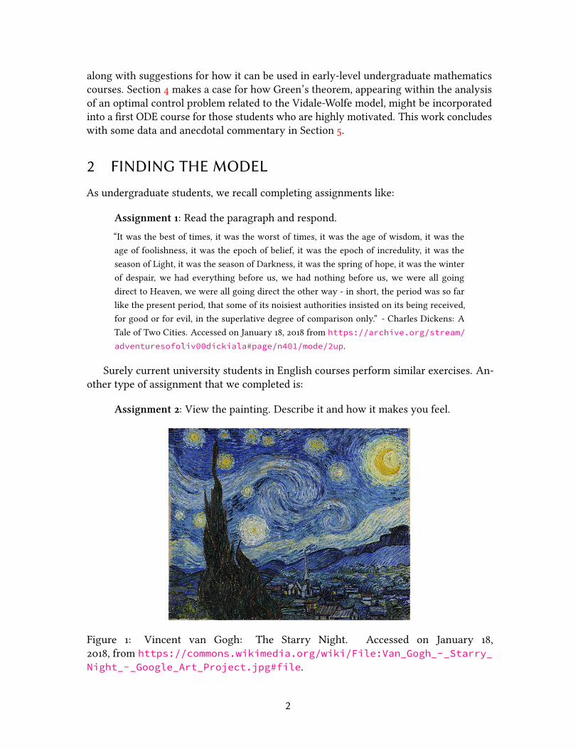
Assignment 2: View the painting. Describe it and how it makes you feel.

Figure 1: Vincent van Gogh: The Starry Night. Accessed on January 18,2018, from https://commons.wikimedia.org/wiki/File:Van_Gogh_-_Starry_Night_-_Google_Art_Project.jpg#file.

2

On the other hand, we venture to say that most of our students have probably notundertaken an exercise such as:

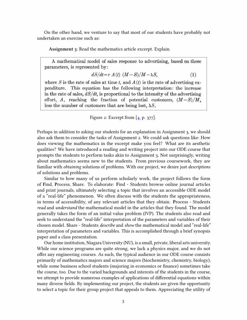
Assignment 3: Read the mathematics article excerpt. Explain.

Figure 2: Excerpt from [4, p. 377].

Perhaps in addition to asking our students for an explanation in Assignment 3, we shouldalso ask them to consider the tasks of Assignment 2. We could ask questions like: Howdoes viewing the mathematics in the excerpt make you feel? What are its aestheticqualities? We have introduced a reading and writing project into our ODE course thatprompts the students to perform tasks akin to Assignment 3. Not surprisingly, writingabout mathematics seems new to the students. From previous coursework, they arefamiliar with obtaining solutions of problems. With our project, we desire just descriptionsof solutions and problems.

Similar to how many of us perform scholarly work, the project follows the formof Find, Process, Share. To elaborate: Find - Students browse online journal articlesand print journals, ultimately selecting a topic that involves an accessible ODE modelof a “real-life” phenomenon. We often discuss with the students the appropriateness,in terms of accessibility, of any relevant articles that they obtain. Process - Studentsread and understand the mathematical model in the articles that they found. The modelgenerally takes the form of an initial value problem (IVP). The students also read andseek to understand the “real-life” interpretation of the parameters and variables of theirchosen model. Share - Students describe and show the mathematical model and “real-life”interpretation of parameters and variables. This is accomplished through a brief synopsispaper and a class presentation.

Our home institution, Niagara University (NU), is a small, private, liberal arts university.While our science programs are quite strong, we lack a physics major, and we do notoffer any engineering courses. As such, the typical audience in our ODE course consistsprimarily of mathematics majors and science majors (biochemistry, chemistry, biology),while some business school students (majoring in economics or finance) sometimes takethe course, too. Due to the varied backgrounds and interests of the students in the course,we attempt to provide numerous examples of applications of differential equations withinmany diverse fields. By implementing our project, the students are given the opportunityto select a topic for their group project that appeals to them. Appreciating the utility of

3

ODEs is a wonderful by-product of the project. However, the main goal of the project isto enhance students’ mathematical communication ability. This includes improving theirreading comprehension and their ability to explain mathematics through both writingand speaking.

The project is designed to parallel the content development in the course. Deadlinesfor the different parts of the project are carefully chosen throughout the semester so thatstudents in the course will have had a chance to learn any relevant mathematics prior tosubmitting their project work. The assessment of the group project consists of gradinga group topic proposal for completeness, grading the short paper, and evaluating thepresentation. Based on preliminary analysis of course and exam scores, the project isassociated with improved individual performance in the course, including an increasein content comprehension. The project has seen some major and minor successes, butis constantly undergoing refinement for improvement in future semesters. One majorsuccess of the project is that it led a team of students to pursue further study on theirtopic, the Vidale-Wolfe marketing model. By locating Vidale and Wolfe [4], these twostudents “discovered” the Vidale-Wolfe marketing model, and they created an excellentcourse project. As a consequence, we too found the Vidale-Wolfe model.

3 PROCESSING THE VIDALE-WOLFE MODEL

As we discussed the Vidale-Wolfe marketing model with our students, it became apparentthat it contained much interesting mathematics. In this section, we delve further into thismodel to show how it can serve as a fresh example of various mathematical techniques ina first ODE course.

3.1 The Model

In an effort to understand advertising expenditure and sales, Vidale and Wolfe developeda differential equation model capable of measuring the effectiveness of advertising cam-paigns for the companies and products that they considered in Vidale andWolfe [4]. Otherquestions that they sought to answer, and that relied on a quantitative understanding ofthe effectiveness of an advertising campaign, concerned allocation of resources amongstmultiple products and determining an appropriate size for an advertising budget. Theirwork was extended by other researchers (see Sethi [2] and the references therein). Ofparticular note, the work in Sethi [2] provides optimal controls for the Vidale-Wolfemarketing model by developing various optimal advertising strategies. Section 4 of thiswork will discuss some of those details.

The original model proposed by Vidale and Wolfe in 1957 is a first-order, linear, non-homogeneous ordinary differential equation with an initial condition. The IVP is

dS

dt= rA(t)

(M − S

M

)− λS, S(0) = S0

where the dependent variable, S = S(t), is the rate of sales at time t . The initial rate of salesis a constant, S(0) = S0. The inhomogeneity, i.e., the forcing term, is rA(t), where A(t) is

4

the rate of advertising expenditure and r is a response constant. The other parameters areM , the saturation level, and λ, a sales decay constant. While we refer the interested readerto Vidale and Wolfe [4] for a complete description of these quantities, our students areexpected to give further explanation about the variables and parameters in their project,including units. For example, they might explain how M , in units of dollars per month,is determined for a particular product within the article and what real-life quantity itrepresents. Groups might present information like in Figure 2, where Vidale and Wolfepoint out that the increase in the rate of change of sales, i.e., dSdt , is proportional to theadvertising expenditure and the fraction of potential customers M−S

M . The increase islessened by a loss of customers, reflected in the term λS for λ > 0. In other words, salesdecrease at an exponential rate of λ in the absence of advertising.

3.2 The Features

In the remainder of this work, we consider a scaled version of the model, following Sethi[2]. In Sethi’s notation, the scaled problem is

dx

dt= ρu(t)(1 − x) − kx, x(0) = x0 (3.1)

where x = S/M is market share with initial constant value x(0) = x0. The responseconstant is ρ = r/M , advertising is u = A, and k = λ. In Vidale and Wolfe [4], twodifferent advertising strategies are considered: constant advertising over a finite timeinterval and pulse advertising. Pulse advertising is a very large magnitude campaign ofbrief duration. Including a discussion of how the model reacts to these different advertisinginputs is instructive for a first ODE course.

Suppose the constant advertising strategy is given by

u(t) =

{u if 0 ≤ t ≤ τ0 if t > τ

(3.2)

where u > 0 is constant and τ > 0 is the constant length of the advertising campaign.Using standard methods from a first ODE course (perhaps the method of integratingfactors), one can compute a solution to (3.1). A representative trajectory is depicted inFigure 3(a) for illustrative parameter values t ∈ [0, 12], τ = 6, u = 1, ρ = 0.25, k = 0.1,and x0 = 0.2. The solution is quite similar to that encountered in break-point models thatstudents in a first ODE course learn about in the context of ODEs for the velocity in airresistance/parachute models or ODEs in compartmental mixing models (see, e.g., Nagleet al. [1], Exercise 7, p. 122). We provide a simple example. Suppose that, for 10 seconds, asalt solution of concentration 1

2 kg/L is pumped into a large tank containing 1L of purewater at a rate of 1 L/sec. At the same time, assuming the tank is kept well-mixed, solutionis pumped out of the tank at a rate of 1 L/sec. After these initial 10 seconds, pure water ispumped into the tank at a rate of 1

2 L/sec and the solution is pumped out at a rate of 12

L/sec. If y(t) is the amount of salt in the tank at time t , this scenario can be modeled by

5

10 120 2 4 6 80

0.2

0.4

0.6

0.8

1

00

(a) (b)

Figure 3: (a) Solution, x(t), in constant advertising case. (b) Advertising pulse.

two ODEs similar to (3.1) with u(t) given by (3.2).

First 10 seconds Next 10 secondsdy

dt= 1

2 − ydy

dt= −1

2y

This is (3.1) with ρu = 12,k =

12 . This is (3.1) with u = 0,k = 1

2 .

For students whose interests lean more toward business, the Vidale-Wolfe model providesa more relevant application of such a break-point situation.

Another topic often studied in a first ODE course is pulse forcing. In past courses wehave introduced the idea of a pulse by suggesting that a mass-spring system be set intomotion by a quick hammer strike to the mass. This scenario from the realm of physicsmight be easy for some students to visualize, but we posit that marketing students wouldbe more likely to appreciate an application where the pulse occurs within a sales responsemodel. Figure 3(b) shows a square wave representing an advertising pulse of magnitudeu and duration t+ − t , where t+ is a time “just after” t . An immediate and interestingapplication of pulse forcing in the Vidale-Wolfe model is to determine the magnitude of anadvertising pulse that is required in order to increase market share by some predeterminedamount. A result to this end can be found in Lemma 3.1 from Sethi [3], Lemma 3.1, p. 5.We reproduce the lemma here since its consideration leads to additional analysis that wefind important for our students to see.

Lemma 3.1 (Sethi, 1972). Let P(a,b, t) denote the magnitude of an advertising pulse necessaryto increase market share x(t) = a at time t to x(t+) = b at time t+ ( just after t ); then

P(a,b, t) = 1/ρ ln [(1 − a)/(1 − b)] = P(a,b) (3.3)

for all 0 ≤ a ≤ b ≤ 1 and for all t . Furthermore, if a ≤ c ≤ b, then P(a,b, t) = P(a, c, t) +P(c,b, t).

Proof. The idea of the proof is to solve the ODE in (3.1) via definite integration and thentake appropriate limits to represent the behavior of the intense advertising campaignpulse for an extremely short time interval.

6

00

a

x(t+)

1

Figure 4: Total additional market share due to advertising pulse.

Temporarily fixing u and integrating (3.1) from t to t + δt leads to

x(t + δt) = e−(k+ρu)δta + e−(k+ρu)(t+δt)ρu∫ t+δt

te(k+ρu)s ds

Evaluating the integral and letting u → ∞, δt → 0, and uδt → P gives

x(t+) = e−ρP (a − 1) + 1

Since x(t+) = b, the first part of the lemma follows readily.The additive property in the lemma is a simple exercise using algebraic properties of

logarithms. �

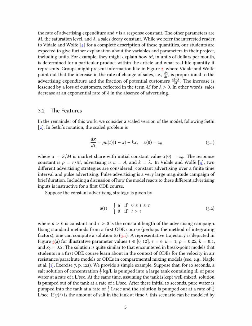
Some additional quantities of interest can be computed with the aid of Lemma 3.1. Inparticular, Vidale and Wolfe show that the immediate market share increase due to theadvertising pulse is

x(t+) − a = (1 − a)(1 − e−ρP )Moreover, the total additional market share generated by the pulse campaign is∫ ∞

0(x(t+) − a)e−kt dt =

(1 − a)

k(1 − e−ρP ) ≈

ρP

k(1 − a) (3.4)

if sales are small compared to saturation level (see Vidale andWolfe [4], p. 378). In (3.4), wehave a nice use of an improper integral. Visually, our students appreciate the computationas the area of the “infinite” shaded region in Figure 4, where the curves are x(t+)e−ktand ae−kt . From an instructional point of view, we are certainly getting excited aboutthe wonderful mathematics that has arisen in our analysis of the Vidale-Wolfe model.Indeed, we have even used a Taylor polynomial approximation to an exponential functionin (3.4), i.e., e−ρP ≈ 1− ρP . Perhaps one could use this example instead of small amplitudeestimations in pendulum analysis (see, e.g., Nagle et al. [1], p. 226). Thus, the Vidale-Wolfemodel provides yet another benefit for our students who lack background in physics.

7

4 OPTIMAL CONTROL AND GREEN’S THEOREM

For those particularly motivated students in our course, we can suggest that the main useof Lemma 3.1 is in specifying an optimal control for the following optimization problem.One wishes to maximize the present value of the profit stream up to horizon T , i.e, overthe time interval [0,T ]. In other words, one attempts to solve

Problem (P): max0≤u(t)≤Q

{J =

∫ T

0(πx − u)e−it dt

}subject to the state equation (3.1) and the fixed endpoint constraint x(T ) = xT . Here, π ismaximum sales revenue potential,Q is maximum allowable rate of advertising expenditure,and i is discount rate. This is a problem in the calculus of variations. Stated another way,we seek an advertising function u(t) that makes the functional J as large as possible, whilex(t) still satisfies the Vidale-Wolfe IVP and the further restriction that the total marketshare at time T is fixed at a predetermined level, i.e., x(T ) = xT .

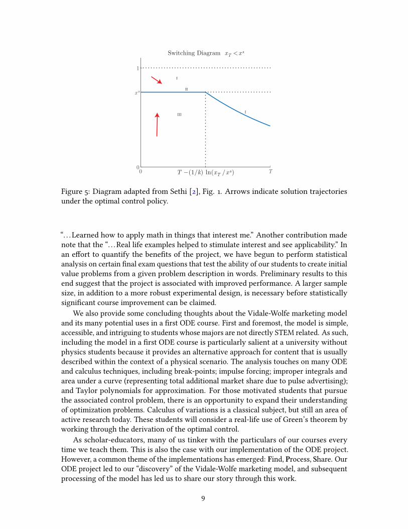
In Winkel [5], another author points out how an optimal control problem related tothe number of worker and queen bees in a colony can find a place in an ODE course withan emphasis on modeling. Our problem is similar. Indeed, Sethi first constructs an optimalstrategy using a combination of pulsing, singular control, and bang-bang control in thecase when Q = ∞, i.e., when the advertising strategy need not be bounded. The details ofthe solution follow from Green’s theorem and are accessible, with some work, to our beststudents. We present some of the details in the Appendix. Through the analysis, one isled to a switching diagram like Figure 5, where xs is a constant market share dependingon k, i, π , and ρ that arises in the analysis of Problem (P). The formula for xs is given inthe Appendix. The corresponding control is us , obtained by solving for u in (3.1) aftersetting dx

dt = 0 and x = xs . Three portions of the tx-plane are identified and labeled asI , I I , and I I I .

I = {(t, x) | xs < x < 1, 0 < t < T } ∪ {(t, x) | T − 1k ln (xT /x

s) ≤ t < T , x =x2s

xTe−k(t−T )}

I I = {(t, x) | x = xs, 0 < t < T − 1k ln (xT /x

s)}

I I I = {(t, x) | 0 < t < T − 1k ln (xT /x

s), 0 < x < xs}

While the details are best left to the interested reader, we point out the following idea ofthe switching diagram and optimal advertising policy. If (t, x) ∈ I I I , apply pulses untilreaching xs . Then applyus to maintain xs until advertising is halted at timeT − 1

k ln (xT /xs)

in order to meet the target xT . When (t, x) ∈ I , advertising is halted, i.e., u = 0. Theoptimality of this advertising strategy is established in Sethi [3], p. 6-7.

5 SHARING THE MODEL AND CONCLUSIONS

We begin with some concluding thoughts about the reading and writing ODE project.Students found many refreshingly different models with broad appeal, an important pointconsidering that NU does not have a physics major. Commentary from course evaluationssupports our observations about the appeal and utility of the project. A student wrote: [I]

8

0 T0

xs

1

Switching Diagram xT <xs

III

I

II

I

T −(1/k) ln(xT /xs)

Figure 5: Diagram adapted from Sethi [2], Fig. 1. Arrows indicate solution trajectoriesunder the optimal control policy.

“. . . Learned how to apply math in things that interest me.” Another contribution madenote that the “. . . Real life examples helped to stimulate interest and see applicability.” Inan effort to quantify the benefits of the project, we have begun to perform statisticalanalysis on certain final exam questions that test the ability of our students to create initialvalue problems from a given problem description in words. Preliminary results to thisend suggest that the project is associated with improved performance. A larger samplesize, in addition to a more robust experimental design, is necessary before statisticallysignificant course improvement can be claimed.

We also provide some concluding thoughts about the Vidale-Wolfe marketing modeland its many potential uses in a first ODE course. First and foremost, the model is simple,accessible, and intriguing to students whose majors are not directly STEM related. As such,including the model in a first ODE course is particularly salient at a university withoutphysics students because it provides an alternative approach for content that is usuallydescribed within the context of a physical scenario. The analysis touches on many ODEand calculus techniques, including break-points; impulse forcing; improper integrals andarea under a curve (representing total additional market share due to pulse advertising);and Taylor polynomials for approximation. For those motivated students that pursuethe associated control problem, there is an opportunity to expand their understandingof optimization problems. Calculus of variations is a classical subject, but still an area ofactive research today. These students will consider a real-life use of Green’s theorem byworking through the derivation of the optimal control.

As scholar-educators, many of us tinker with the particulars of our courses everytime we teach them. This is also the case with our implementation of the ODE project.However, a common theme of the implementations has emerged: Find, Process, Share. OurODE project led to our “discovery” of the Vidale-Wolfe marketing model, and subsequentprocessing of the model has led us to share our story through this work.

9

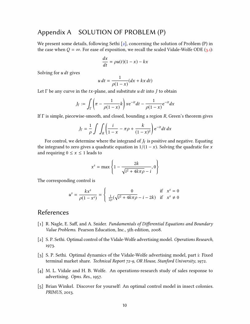
Appendix A SOLUTION OF PROBLEM (P)

We present some details, following Sethi [2], concerning the solution of Problem (P) inthe case when Q = ∞. For ease of exposition, we recall the scaled Vidale-Wolfe ODE (3.1):

dx

dt= ρu(t)(1 − x) − kx

Solving for u dt givesu dt =

1ρ(1 − x)

(dx + kx dt)

Let Γ be any curve in the tx-plane, and substitute u dt into J to obtain

JΓ :=∫Γ

(π −

1ρ(1 − x)

k

)xe−itdt −

1ρ(1 − x)

e−itdx

If Γ is simple, piecewise-smooth, and closed, bounding a region R, Green’s theorem gives

JΓ =1ρ

∫ ∫R

(i

1 − x− πρ +

k

(1 − x)2

)e−itdt dx

For control, we determine where the integrand of JΓ is positive and negative. Equatingthe integrand to zero gives a quadratic equation in 1/(1 − x). Solving the quadratic for xand requiring 0 ≤ x ≤ 1 leads to

xs = max

{1 −

2k√i2 + 4kπρ − i

, 0

}The corresponding control is

us =kxs

ρ(1 − xs)=

{0 if xs = 0

12ρ (

√i2 + 4kπρ − i − 2k) if xs , 0

References

[1] R. Nagle, E. Saff, and A. Snider. Fundamentals of Differential Equations and BoundaryValue Problems. Pearson Education, Inc., 5th edition, 2008.

[2] S. P. Sethi. Optimal control of the Vidale-Wolfe advertising model. Operations Research,1973.

[3] S. P. Sethi. Optimal dynamics of the Vidale-Wolfe advertising model, part i: Fixedterminal market share. Technical Report 72-9, OR House, Stanford University, 1972.

[4] M. L. Vidale and H. B. Wolfe. An operations-research study of sales response toadvertising. Opns. Res., 1957.

[5] Brian Winkel. Discover for yourself: An optimal control model in insect colonies.PRIMUS, 2013.

10