Financial Frictions, Asset Prices, and the Great Recessionvr0j/slides/vzuhouston.pdf · Financial...

Financial Frictions, Asset Prices, and theGreat Recession

Zhen Huo and Jose-Vıctor Rıos-Rull

New York University, University of Pennsylvania, UCL, CAERP

University of Houston

Monday 4th April, 2016

First Version April 2013

Huo & Rıos-Rull, NYU, Penn, UCL, CAERP Financial Frictions, Asset Prices, & the Great Recession University of Houston 1/60

We have had a Great Recession

• Both in the U.S. and in (mostly Southern) Europe

Large decline in output, employment, consumption, and investment.

Households deleveraging process: private debt and housing pricesplunged.

Total factor productivity (TFP) dropped.


Facts on the last recession: output, unemp, cons, inv

2002 2004 2006 2008 2010 2012 2014 2016−8

−6

−4

−2

0

2

4

6

8

Real output

2002 2004 2006 2008 2010 2012 2014 20164

5

6

7

8

9

10

Unemployment rate

2002 2004 2006 2008 2010 2012 2014 2016−10

−8

−6

−4

−2

0

2

4

6

8

Consumption

2002 2004 2006 2008 2010 2012 2014 2016−40

−30

−20

−10

0

10

20

30

Investment

Note: Except for unemployment, figures show percentage deviation from a linear trend.


Facts on the last recession: wealth, mortg, houses, pr h

2002 2004 2006 2008 2010 2012 2014 20163.8

4

4.2

4.4

4.6

4.8

5

Net worth to output

2002 2004 2006 2008 2010 2012 2014 20160.5

0.55

0.6

0.65

0.7

0.75

Mortgage debt to output

2002 2004 2006 2008 2010 2012 2014 20161.1

1.2

1.3

1.4

1.5

1.6

1.7

1.8

1.9

Housing value to output

2002 2004 2006 2008 2010 2012 2014 2016150

160

170

180

190

200

210

220

230

Housing price index


Facts on the last recession: productivity and labor quality

2002 2004 2006 2008 2010 2012 2014 2016−4

−3

−2

−1

0

1

2

3

4

5

6

TFP: measured with total hours

2002 2004 2006 2008 2010 2012 2014 2016−8

−6

−4

−2

0

2

4

6

Labor productivity

2002 2004 2006 2008 2010 2012 2014 2016−1

−0.8

−0.6

−0.4

−0.2

0

0.2

0.4

0.6

0.8

Labor force quality

2009 2010 2011 2012 2013 2014 2015−4.5

−4

−3.5

−3

−2.5

−2

−1.5

−1

−0.5

0

0.5

TFP: measured with total hoursTFP: measured with total labor inputs


Culprit: Financial Shocks?

When looking for triggers of the Great Recession some form offinancial breakdown comes out in most popular explanations.

Financing difficulties contribute to cut spending both of firms andhouseholds.

Most of the action occurs via a demand reduction.

Yet models have a hard time to deliver this.


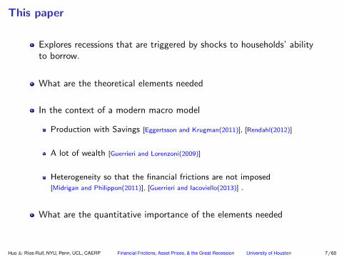
This paper

Explores recessions that are triggered by shocks to households’ abilityto borrow.

What are the theoretical elements needed

In the context of a modern macro model

Production with Savings [Eggertsson and Krugman(2011)], [Rendahl(2012)]

A lot of wealth [Guerrieri and Lorenzoni(2009)]

Heterogeneity so that the financial frictions are not imposed[Midrigan and Philippon(2011)], [Guerrieri and Iacoviello(2013)] .

What are the quantitative importance of the elements needed


Findings: The answer is yes, provided there are (from +to-)

1 Real frictions that difficult the switch from production of consumptiongoods to exports or investment.

2 Houses which are inferior goods and not wanted by the super-rich.

3 Frictions in the goods markets that generate movements in measuredGDP.

4 Households that differ in job prospects.

5 Some labor market frictions that limit wage adjustments.


Findings: The Recession that we generate

• Shares most of the features of the Great Recession:

1 A large decline in output, employment, consumption and investment.

2 Large reductions in assets (housing and stocks) prices.


Model


The Model Characteristics: Steady State

Enhanced Aiyagari Economy:

1 Multisector: Tradables and nontradables.

2 Houses (land) that need to be purchased to be enjoyed.

3 Endogenous productivity movements (frictions in goods markets).

4 Various job market frictions.


Households: Preferences

Continuum of households that live forever (β), are subject touninsurable idiosyncratic.

H’holds care about quantities and number of varieties of nontradables.

cN =

(∫ IN

0

c1ρ

Ni di

)ρ= cNi IρN

Households have to search for varieties, its number is a choice.

IN = d Ψd(Qg)

Ψd(Qg): Probability (per search unit) of finding a variety (goods marketfrictions).

Households also like tradables and housing and dislike goods searching

u [cA(cN IρN , cT ), h, d]


Households: Endowments and Wealth

Household skill type is ε, follows a Markov chain Γε,ε′ . Moves slowlyand accommodates opportunities to get rich.

Households either have a job e = 1 or not e = 0.

Type-dependent exogenous job destruction rate δεn.

Job finding rate is type independent and depends on job creation byfirms (workers are rationed, it is like no matching function in labormarket but hiring costs) ([Fang and Nie(2013)] ).

Households have assets a. These assets can be allocated to(frictionless) houses and/or to financial assets with a collateralconstraint. The poor will have some housing wealth and a mortgage,the rich houses and shares of the economy’s mutual fund.


Goods markets

Search frictions in the markets for nontradables:

Households look for varieties.

Random search.

Richer people consume and search more.

Cuts in consumption cut search which cuts productivity.

Perfect competition and frictionless markets for tradables.


Labor market

Workers are rationed.

Firms hire as many workers as they wish paying hiring costs. (like avacancy filling probability of 1, with hiring costs).

Employment: N = NN +NT .

Same job finding probability across types: Φe = V1−N .

Wages are exogenous (set to some aggregate target).


Assets markets: Financial assets and houses

Total housing H is in fixed supply.

Negative financial assets (b′ < 0) are (undefaultable) mortgages.

Its interest rate is predetermined: 11+r∗ − ς, if b < 0.

Mortgages have to be collateralized by housing: if b < 0 then

|b| ≤ [1− λ] ph h

[1

1 + r∗− ς]

Positive financial assets (b > 0) are shares of a mutual fund.

Its return, r, is determined ex-post (it matters when we hit the economywith shocks). Possible capital gains and loses.

R(b) =

1 + r, if b ≥ 01, if b < 0.


Households’ problem

V (ε, e, a) = maxcN,i,cT ,IN ,h,d

u(cA, h, d)+

β∑ε′,e′,θ′

Πθθ,θ′ Π

we′|e,ε Πε

ε,ε′ V [ε′, e′, a′(b, h)] s.t.

∫ IN

0

picN,i + cT + phh+ b = a+ 1e=1wε+ 1e=0 w BC

a′(b, h) = phh+R(b)b AA

b ≥ −λ ph h[

1

1 + r∗− ς

]FC

IN = d Ψd[Qg] SC


Nontradables: Monopolistic Competition by Varieties

Each firm/variety has any locations each.

Some inputs are location specific. Others (type 2 labor) are not.

Prices are posted before location is filled

The demand function is given by

Ψf [Qg]

∫c[pi(ε, e, a), x] d(x, S)

The firm has to make sure that it can satisfy the demand at alllocations.


Nontradable firms’ problem

ΩN (k, n) = maxi,v,pi`1,`2

Ψf [Qg]pi

∫c(pi, ε, e, a) dx− w`− i− κv

+∑θ′

Πθθ,θ′

ΩN (k′, n′)

1 + r∗

subject to

`2 ≥ Ψf [Qg]

∫f `[c(pi, x), k, `1]

d(x, S)

DDC

`1 + `2 = nε SL

k′ = (1 − δk)k + i− φN (k, i) LMK

n′ = [1 − δn]n+ v LML


Tradable firms’ are competitive and have adjustment costs

• Its output is used for exports, investment, and (part of) consumption.• Decreasing returns.

ΩT (k, n) = maxi,v

FT (k, `) − w`− i− κv − φT,n(n′, n)

+∑θ′

Πθθ,θ′

ΩT (k′, n′)

1 + r∗

subject to

k′ = (1 − δk)k + i− φT,k(k, i)

` = nε

n′ = [1 − δn]n+ v


Mutual fund

Financial wealth in the economy is

L+ =

∫b>0

b(ε, e, a) dx

Mortgages in the economy are

L− =

∫b<0

−b(ε, e, a) dx

Net foreign asset position of the country (the mutual fund owns allfirms)

B = L+ −(

ΩN − πN + ΩT − πT +1

1 + r∗L−

)The realized rate of return is

1 + r =ΩN + ΩT + (1 + r∗)B + L−

L+


EquilibriumAn equilibrium is a set of decision rules and values for households, firms’values and decision rules, and a set aggregate variables of aggregatestates, such that:

Households’ and firms’ policy functions and value functions solve thecorresponding program problems.

Aggregate searching consistence

D =

∫d(ε, e, a) dx,

Nontradable prices satisfies

p = pi(KN , NN ) dx,

Housing market clears ∫h(ε, e, a) dx = H.


Equilibrium

Average separation probability and labor force quality

δn =

∑ε δn(ε)n(ε)

N, ε =

∑ε εn(ε)

N

Rate of return to the mutual fund satisfies

1 + r =ΩN + ΩT + (1 + r∗)B +

∫b<0

b(x)∫b>0

b(x)


The Financial Shocks

We now pose simultaneous shocks to the Financial system: Both to

1 Loan to value ratio. λ

2 Markup on loans ζ

Two options to solve for out of steady State

1 MIT shocks. A surprise and track the transition to a new steady State

2 Pose a known stochastic process and solve it via a Krusell-Smith typemethod.

We do the first.


Solve for the transition

We have to take care of wages dynamics.They are determined via the following formula

logw − logw = εw(logY − logY

)

It simplifies things.[Gornemann, Kuester, and Nakajima(2012)].

We have to take care of solving for the transition which implies solvingfor sequences for home prices, wages, nontradable prices.

We assume the transition is completed in T periods.


Mapping the Model to Data


Functional forms

Preferences

u(cA, h, d) =1

1 − σc

(cA − ξd

d1+γ

1 + γ

)1−σc+ v(h)

where there is an Armington aggregator for consumption

cA =

[ω (cN IρN )

η−1η + (1 − ω)c

η−1η

T

] ηη−1

and houses are inferior goods as a proxy for segmentation of housingmarkets

v(h) =

ξh log(h), if h < h1ξh

1−σhh1−σh , if h1 ≤ h ≤ h2.

ξh√h− h, if h > h2.


Housing Utility Function

Housing utility function Engel Curve: consumption vs housing

0 1 2 3 4 5−1.2

−1

−0.8

−0.6

−0.4

−0.2

0

0.2

0.4

Housing

Housingutility

1 2 3 4 5 6 7 82.5

3

3.5

4

4.5

5

Consumption

Housing


Functional forms

Production function

FN (k, `1, `2) = zN kα0 `α11 `α2

2 , FT (k, `) = zT kθ0`θ1

Capital adjustment cost in the nontradable goods sector

φN (i, k) =ψ

2

(i

k− δk

)2

k

Capital and employment adjustment cost in the tradable goods sector

φT,k(i, k) =ψ

2

(i

k− δk

)2

k, φT,n(n′, n) =ψ

2

(n′

n− 1

)2

n

Matching technology

M(D,T ) = νDµT 1−µ


Exogenously determined parameters

Parameter Value

Risk aversion for consumption, σc 2.0

Satiation level for housing, h 5.0

Curvature of shopping, γ 1.5

Elasticity of substitution bw tradables and nontradables, η 0.80

Price markup, ρ 1.1

Loan to value ratio, λ 0.80

Interest rate for international bonds, r∗ 4%

Note: model period is half a quarter


Endogenously determined parameters: aggregateTarget Value Parameter Value

Wealth to output ratio 4.00 β 0.97

Housing value to output ratio 1.70 ξh 0.54

Debt to output ratio 0.40 ε4 37.41

Fraction of housing held by bottom 70% 0.25 h1 1.48

Fraction of housing held by bottom 80% 0.39 h2 4.22

Fraction of housing held by bottom 90% 0.58 σh 2.92

Share of tradables 0.30 ω 0.98

Occupancy Rate 0.81 ν 0.81

Capital to output ratio 2.00 δk 0.01

Labor Share in nontradables 0.64 α0 0.27

α1 = α2 —— α1 0.36

Labor Share in tradables 0.66 θ1 0.66

Vacancy cost to output ratio 0.02 κ 0.42

Home production to lowest earning ratio 0.50 w 0.07

Units Parameters

Output 1 zN 0.93

Relative price of nontradables 1 zT 0.48

Market tightness in goods markets 1 ξd 0.03


Endogenously determined parameters: cross-section Lorenz

Target Value Parameter Value

Job duration for type 1 1.5 year δ1n 0.083

Job duration for type 3 5 year δ3n 0.025

Job duration for type 4 5 year δ4n 0.025

Unemployment rate 6% δ2n 0.048

Wealth Gini index 0.82 Πε1,4 0.0007

Earnings Gini index 0.64 Πε4,1 0.0058

Earning autocorrelation 0.91 Πε1,1 0.9656

Earning stdev 0.20 Πε2,2 0.9770


Lorenz Curve Return

Networth Housing

0 0.1 0.2 0.3 0.4 0.5 0.6 0.7 0.8 0.9 1

0.1

0.2

0.3

0.4

0.5

0.6

0.7

0.8

0.9

1

ModelData

0 0.1 0.2 0.3 0.4 0.5 0.6 0.7 0.8 0.9 1

0.1

0.2

0.3

0.4

0.5

0.6

0.7

0.8

0.9

1

ModelData


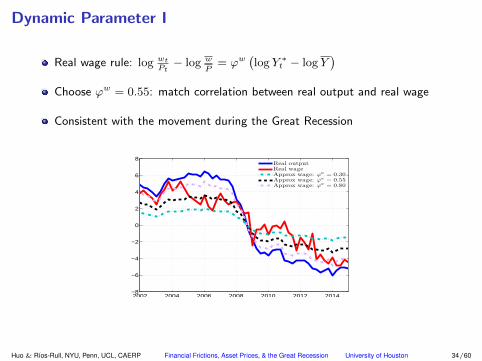
Dynamic Parameter I

Real wage rule: log wtPt− log w

P= ϕw

(log Y ∗

t − log Y)

Choose ϕw = 0.55: match correlation between real output and real wage

Consistent with the movement during the Great Recession

2002 2004 2006 2008 2010 2012 2014−8

−6

−4

−2

0

2

4

6

8

Real outputReal wageApprox wage: ϕw = 0.30Approx wage: ϕw = 0.55Approx wage: ϕw = 0.80


Dynamic Parameter II

Summary of Dynamic Parameters

Parameter Value Target

Adjustment cost, ψ 1.60 Decrease in investment: 30%

DRS in tradables, θ0 0.21 Increase in tradable sector: 4%

Goods market matching elasticity in, µ 0.80 Decrease in TFP: 1.5%

Wage elasticity, ϕw 0.55 Ratio of wage to output change: 0.55


Experiments: once and for all set of surprises

1 Baseline

Over three months the down payment changes from 20% to 40%

The borrowing interest rate’s surcharge goes from zero to 0.5%

2 Decomposition: with only down payment or interest rate change

3 Role of asset price: constant housing price

4 Role of frictions: wage elasticity, matching frictions and adj costs

5 Allowing default: a larger drop of housing price

6 Credit cycle


Long Run Properties

• Typically like in all [Aiyagari(1994)] - [Bewley(1986)] -[Huggett(1993)] - [Imrohoroglu(1989)] type models, in the long runoutput and wealth end up being higher.

• But in our economies the transition is associated to a recession.


Experiment 1: Baseline

0 1 2 3 4 5 6 7 8 9 10−3.5

−3

−2.5

−2

−1.5

−1

−0.5

0

Baseline

Real output

0 1 2 3 4 5 6 7 8 9 106

6.5

7

7.5

8

8.5

9

Baseline

Unemployment

0 1 2 3 4 5 6 7 8 9 10−7

−6

−5

−4

−3

−2

−1

0

Baseline

Consumption

0 1 2 3 4 5 6 7 8 9 10−30

−25

−20

−15

−10

−5

0

5

Baseline

Investment



0 1 2 3 4 5 6 7 8 9 10−8

−7

−6

−5

−4

−3

−2

−1

0

Baseline

Wealth

0 1 2 3 4 5 6 7 8 9 10−35

−30

−25

−20

−15

−10

−5

0

Baseline

Debt

0 1 2 3 4 5 6 7 8 9 10−18

−16

−14

−12

−10

−8

−6

−4

−2

0

Baseline

Housing price



0 1 2 3 4 5 6 7 8 9 10−1.5

−1

−0.5

0

Baseline

TFP with total hours

0 1 2 3 4 5 6 7 8 9 10−1.5

−1

−0.5

0

Baseline

Labor Productivity

0 1 2 3 4 5 6 7 8 9 100

0.2

0.4

0.6

0.8

1

1.2

1.4

Baseline

Labor quality

0 1 2 3 4 5 6 7 8 9 10−2.5

−2

−1.5

−1

−0.5

0

Baseline

TFP with total labor inputs


Experiment 2 : Only λ or r Change

0 1 2 3 4 5 6 7 8 9 10−3.5

−3

−2.5

−2

−1.5

−1

−0.5

0

BaselineOnly λ changeOnly r change

0 1 2 3 4 5 6 7 8 9 106

6.5

7

7.5

8

8.5

9


Real output Unemployment rate

0 1 2 3 4 5 6 7 8 9 10−1.6

−1.4

−1.2

−1

−0.8

−0.6

−0.4

−0.2

0

0.2


0 1 2 3 4 5 6 7 8 9 10−18

−16

−14

−12

−10

−8

−6

−4

−2

0


TFP Housing price


Experiment 3: with Constant Housing Price

0 1 2 3 4 5 6 7 8 9 10−3.5

−3

−2.5

−2

−1.5

−1

−0.5

0

0.5

BaselineConstant housing price

0 1 2 3 4 5 6 7 8 9 105.5

6

6.5

7

7.5

8

8.5

9



0 1 2 3 4 5 6 7 8 9 10−1.6

−1.4

−1.2

−1

−0.8

−0.6

−0.4

−0.2

0

0.2


0 1 2 3 4 5 6 7 8 9 10−18

−16

−14

−12

−10

−8

−6

−4

−2

0


TFP Housing price


Experiment 4.1: Wage Elasticity

0 1 2 3 4 5 6 7 8 9 10−3.5

−3

−2.5

−2

−1.5

−1

−0.5

0

BaselineHigh wage elasticity: ϕw = 1.0

0 1 2 3 4 5 6 7 8 9 106

6.5

7

7.5

8

8.5

9



0 1 2 3 4 5 6 7 8 9 10−1.6

−1.4

−1.2

−1

−0.8

−0.6

−0.4

−0.2

0


0 1 2 3 4 5 6 7 8 9 10−18

−16

−14

−12

−10

−8

−6

−4

−2

0


TFP Housing price


Experiment 4.2: Adjustment Cost

0 1 2 3 4 5 6 7 8 9 10−3.5

−3

−2.5

−2

−1.5

−1

−0.5

0

BaselineLow adjustment cost

0 1 2 3 4 5 6 7 8 9 106

6.5

7

7.5

8

8.5

9



0 1 2 3 4 5 6 7 8 9 10−2

−1.8

−1.6

−1.4

−1.2

−1

−0.8

−0.6

−0.4

−0.2

0


0 1 2 3 4 5 6 7 8 9 10−18

−16

−14

−12

−10

−8

−6

−4

−2

0


TFP Housing price


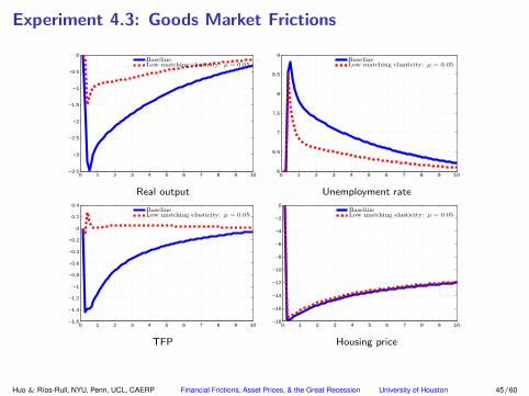
Experiment 4.3: Goods Market Frictions

0 1 2 3 4 5 6 7 8 9 10−3.5

−3

−2.5

−2

−1.5

−1

−0.5

0

BaselineLow matching elasticity: µ = 0.05

0 1 2 3 4 5 6 7 8 9 106

6.5

7

7.5

8

8.5

9



0 1 2 3 4 5 6 7 8 9 10−1.6

−1.4

−1.2

−1

−0.8

−0.6

−0.4

−0.2

0

0.2

0.4


0 1 2 3 4 5 6 7 8 9 10−18

−16

−14

−12

−10

−8

−6

−4

−2

0


TFP Housing price


Experiment 5: Allowing Households Holding no Housing

30% of households hold zero houses in the United States

Change preference slightly to match this moment

v(h) =

ξh log(h+ h), if h < h1,ξh

1−σh

(h+ ξ1

h

)1−σh + ξ2h, if h1 ≤ h ≤ h2,

ξ3h

√h

2 − (h− h)2 + ξ4h, if h > h2.

Similar aggregate response, but richer cross-sectional implications


Experiment 5: Aggregate Response

0 1 2 3 4 5 6 7 8 9 10−3.5

−3

−2.5

−2

−1.5

−1

−0.5

0

BaselineExtension: allowing no housing

0 1 2 3 4 5 6 7 8 9 106

6.5

7

7.5

8

8.5

9



0 1 2 3 4 5 6 7 8 9 10−1.5

−1

−0.5

0


0 1 2 3 4 5 6 7 8 9 10−20

−18

−16

−14

−12

−10

−8

−6

−4

−2

0


TFP Housing price


Experiment 5: Cross-Sectional Effects

10 20 30 40 50 60 70 80 90 100−60

−50

−40

−30

−20

−10

0

Wealth

10 20 30 40 50 60 70 80 90 100−16

−14

−12

−10

−8

−6

−4

−2

0

2

4

Consumption

• This agrees with the evidence in [Petev, Pistaferri, and Eksten(2012)] and

[Parker and Vissing-Jorgensen(2009)]


Experiment 6: Allowing Default

Borrowing interest rate’s surcharge goes from zero to 1%.

Housing price drops more than 20%, and agents may be underwater.

Allow borrowers to default, but savers suffer from the capital loss.



Total saving in financial wealth in the economy is

L+,t =

∫b>0

bt(ε, e, a) dx

Mortgages in the economy are

L−,t =

∫b<0

−bt(ε, e, a) dx

Net foreign asset position of the country

Bt = L+,t −(

ΩNt − πNt + ΩTt − πTt +1

1 + r∗L−,t

)The realized rate of return in next period is

1 + rt+1 =ΩNt+1 + ΩTt+1 + (1 + r∗)Bt

L+

−∫b<0

Iph,t+1ht(ε,e,a)+bt(ε,e,a)>0[ph,t+1ht(ε, e, a) + bt(ε, e, a)] dx

L+



0 1 2 3 4 5 6 7 8 9 10−4.5

−4

−3.5

−3

−2.5

−2

−1.5

−1

−0.5

0

BaselineAllow default

0 1 2 3 4 5 6 7 8 9 106

6.5

7

7.5

8

8.5

9

9.5

10



0 1 2 3 4 5 6 7 8 9 10−2.5

−2

−1.5

−1

−0.5

0


0 1 2 3 4 5 6 7 8 9 10−25

−20

−15

−10

−5

0


TFP Housing price


Experiment 7: Credit Cycle

0 1 2 3 4 5 6 7 8 9 100.55

0.6

0.65

0.7

0.75

0.8

0.85

Loan to value ratio λ


Experiment 7: Credit Cycle

0 1 2 3 4 5 6 7 8 9 10−2.5

−2

−1.5

−1

−0.5

0

0.5

1

1.5

0 1 2 3 4 5 6 7 8 9 104.5

5

5.5

6

6.5

7

7.5

8


0 1 2 3 4 5 6 7 8 9 10−1.2

−1

−0.8

−0.6

−0.4

−0.2

0

0.2

0.4

0.6

0.8

0 1 2 3 4 5 6 7 8 9 10−5

0

5

10

15

20

TFP Housing price


Conclusions

We have a recession generated purely by increased difficulties toborrow on the part of households

The recession comes together with

TFP loses

Drop in Housing prices (movements too sharp because of lack of housefrictions)

Drop in Stock Market

The literature is trying hard to get this ([Midrigan and Philippon(2011)],

[Guerrieri and Lorenzoni(2009)]) with limited success.

Still ways to go:

Foreclosures; slow housing frictions; Long term Mortgages.

Slow expanding export industries.

Model of banking cycles.


Thank you very much


American Time Use Survey Data on Shopping Time

5.2

5.4

5.6

5.8

66.

2

2003 2006 2009 2012Year

Total Shopping Time Trend

1.6

1.8

22.

22.

4

2003 2006 2009 2012Year

Shopping time on services Trend

Total shopping time Shopping time on services


The working of financial shocks that hit the production side

[Bernanke and Gertler(1989)], [Bernanke, Gertler, and Gilchrist(1999)]

Firms cannot borrow as much.

Not all good projects will be undertaken.

Cash rich firms expand at the expense of cash poor firms.

In fact there is some of this in the data: Since 2007 employment of the young

firms went down by 24.5% and in 2012 it was at the historically lowest level.

Firms make themselves vulnerable by being close to their credit limitto improve their bargaining position over wages[Monacelli, Quadrini, and Trigari(2011)]


Why was there a financial shock? (what was the trigger?)

Increased variance in the cross-sectional returns of firms [Bloom(2009)],

[Bloom et al.(2011)Bloom, Floetotto, Jaimovich, and Saporta]

[Arellano, Bai, and Kehoe(2012)], [Christiano, Motto, and Rostagno(2014)] [Dyrda(2015)].

Straight shocks to credit constraints [Jermann and Quadrini(2012)],

[Perri and Quadrini(2011)], [Macera(2015)].


What have we learned

It is hard to get a large recession only from the product side and onlyfrom lower investment.

The largest success (to my knowledge) ([Arellano, Bai, and Kehoe(2012)])

works by having the financial shocks increase the probability of defaultand inducing firms to pursue very conservative use of inputs despitetheir almost normal productivity.

Still it is hard to have a reduction of marginal cash to create a largerecession ([Zetlin-Jones and Shourideh(2012)]).

It may have played a larger role in the expansion of new firms([Dyrda(2015)])


ReferencesAiyagari, S. Rao. 1994.

“Uninsured Idiosyncratic Risk and Aggregate Saving.”Quarterly Journal of Economics 109 (3):659–684.

Arellano, Cristina, Yan Bai, and Patrick J. Kehoe. 2012.

“Financial Frictions and Fluctuations in Volatility.”Federal Reserve Bank of Minneapolis Research Department Sta Report.

Bernanke, B. and M. Gertler. 1989.

“Agency Costs, Net Worth, and Business Fluctuations.”American Economic Review 79 (1):14–31.

Bernanke, Ben S., Mark Gertler, and Simon Gilchrist. 1999.

“The financial accelerator in a quantitative business cycle framework.”In Handbook of Macroeconomics, Handbook of Macroeconomics, vol. 1, edited by J. B. Taylor and M. Woodford, chap. 21.Elsevier, 1341–1393.URL https://ideas.repec.org/h/eee/macchp/1-21.html.

Bewley, Truman. 1986.

“Stationary Monetary Equilibrium with a Continuum of Independently Fluctuating Consumers.”In Contributions to Mathematical Economics in Honor of Gerard Debreu, edited by Werner Hildenbrand and Andreu Mas-Colell.Amsterdam: North Holland.

Bloom, Nicholas. 2009.

“The Impact of Uncertainty Shocks.”Econometrica 77 (3):623–685.URL http://ideas.repec.org/a/ecm/emetrp/v77y2009i3p623-685.html.

Bloom, Nicholas, Max Floetotto, Nir Jaimovich, and Itay Saporta. 2011.

“Really Uncertain Business Cycles.”Mimeo Stanford University.

Christiano, Lawrence, Roberto Motto, and Massimo Rostagno. 2014.

“Risk Shocks.”American Economic Review 104 (1):37–65.

Dyrda, Sebastian. 2015.

“Fluctuations in uncertainty, efficient borrowing constraints and firm dynamics.”Manuscript, University of Minnesota.

Eggertsson, G. and P. Krugman. 2011.

“Debt, deleveraging, and the liquidity trap: a Fisher-Minsky-Koo approach.”Federal Reserve Bank of New York, unpublished manuscript, February.

Fang, Lei and Jun Nie. 2013.

“Education, Human Capital and U.S. Labor Market Dynamics.”Presented at MidWest Macro Meetings.

Gornemann, Nils, Keith Kuester, and Makoto Nakajima. 2012.

“Monetary Policy with Heterogeneous Agents.”Mimeo, FRB Philadelphia.

Guerrieri, Luca and Matteo Iacoviello. 2013.

“Collateral Constraints and Macroeconomic Asymmetries.”Mimeo.

Guerrieri, Veronica and Guido Lorenzoni. 2009.

“Liquidity and Trading Dynamics.”Econometrica 77 (6):1751–1790.

Huggett, Mark. 1993.

“The Risk-Free Rate in Heterogeneous-Agent, Incomplete-Insurance Economies.”Journal of Economic Dynamics and Control 17 (5):953–969.

Imrohoroglu, A. 1989.

“Cost of Business Cycles with Indivisibilities and Liquidity Constraints.”Journal of Political Economy 97 (6):1364–1383.

Jermann, Urban and Vincenzo Quadrini. 2012.

“Macroeconomic Effects of Financial Shocks.”American Economic Review 102 (1):238–71.

Macera, Manuel. 2015.

“Credit Crises and Private Deleveraging.”Unpublished Manuscript, Colorado State University.

Midrigan, V. and T. Philippon. 2011.

“Household Leverage and the Recession.”Working Paper FIN-11-038, New York University.

Monacelli, Tommaso, Vincenzo Quadrini, and Antonella Trigari. 2011.

“Financial Markets and Unemployment.”NBER Working Papers 17389, National Bureau of Economic Research, Inc.URL http://ideas.repec.org/p/nbr/nberwo/17389.html.

Parker, Jonathan A. and Annette Vissing-Jorgensen. 2009.

“Who Bears Aggregate Fluctuations and How?.”American Economic Review 99 (2):399–405.

Perri, Fabrizio and Vincenzo Quadrini. 2011.

“International Recessions.”NBER Working Papers 17201, National Bureau of Economic Research, Inc.URL http://ideas.repec.org/p/nbr/nberwo/17201.html.

Petev, Ivaylo, Luigi Pistaferri, and Itay Saporta Eksten. 2012.

“Consumption and the Great Recession: An analysis of trends, perceptions, and distributional effects.”Analyses of the Great Recession .

Rendahl, P. 2012.

“Fiscal Policy in an Unemployment Crisis.”Working Paper, University of Cambridge.

Zetlin-Jones, Ariel and Ali Shourideh. 2012.

“External Financing and the Role of Financial Frictions over the Business Cycle: Measurement and Theory.”Tech. rep.


https://ideas.repec.org/h/eee/macchp/1-21.html

http://ideas.repec.org/a/ecm/emetrp/v77y2009i3p623-685.html

http://ideas.repec.org/p/nbr/nberwo/17389.html

http://ideas.repec.org/p/nbr/nberwo/17201.html

Financial Frictions, Asset Prices, and the Great Recessionvr0j/slides/vzuhouston.pdf · Financial...

Documents

Transcript of Financial Frictions, Asset Prices, and the Great Recessionvr0j/slides/vzuhouston.pdf · Financial...