FinancialInstitutionsCenter

Financial Fragility, Liquidity and AssetPrices

byFranklin AllenDouglas Gale

01-37-B

The Wharton Financial Institutions Center

The Wharton Financial Institutions Center provides a multi-disciplinary research approach tothe problems and opportunities facing the financial services industry in its search forcompetitive excellence. The Center's research focuses on the issues related to managing riskat the firm level as well as ways to improve productivity and performance.

The Center fosters the development of a community of faculty, visiting scholars and Ph.D.candidates whose research interests complement and support the mission of the Center. TheCenter works closely with industry executives and practitioners to ensure that its research isinformed by the operating realities and competitive demands facing industry participants asthey pursue competitive excellence.

Copies of the working papers summarized here are available from the Center. If you wouldlike to learn more about the Center or become a member of our research community, pleaselet us know of your interest.

Franklin Allen Richard J. HerringCo-Director Co-Director

The Working Paper Series is made possible by a generousgrant from the Alfred P. Sloan Foundation

Financial Fragility, Liquidity and Asset Prices ∗

Franklin AllenDepartment of FinanceWharton School

University of PennsylvaniaPhiladephia, PA 19104

allenf@wharton.upenn.edu

Douglas GaleDepartment of EconomicsNew York University269 Mercer StreetNew York, NY 10003douglas.gale@nyu.edu

January 23, 2003

Abstract

A Þnancial system is fragile if a small shock has a large effect. Sunspotequilibria, where the endogenous variables depend on extrinsic uncer-tainty, provide an extreme illustration. However, fundamental equilibria,where outcomes depend only on intrinsic uncertainty, can also be fragile.We study the relationship between sunspot equilibria and fundamentalequilibria in a model of Þnancial crises. The amount of liquidity is en-dogenously chosen and determines asset prices. The model has multipleequilibria, but only some of these are the limit of fundamental equilibriawhen the fundamental uncertainty becomes vanishingly small. We showthat under certain conditions the only robust equilibria are those in whichextrinsic uncertainty gives rise to asset price volatility and Þnancial crises.

JEL ClassiÞcation: D5, D8, G2

1 Excess sensitivity and sunspots

There are numerous historical examples of Þnancial fragility, where shocks thatare small in relation to the economy as a whole have a signiÞcant impact on theÞnancial system. For example, Kindleberger (1978, pp. 107-108) argues thatthe immediate cause of a Þnancial crisis

∗Earlier versions of this paper were presented at the Cowles Foundation Conference on�The Future of American Banking: Historical, Theoretical, and Empirical Perspectives�, atBoston University, New York University, Northwestern University, the University of Iowa,and the Federal Reserve Bank of Kansas City. We are grateful to the participants for theircomments, particularly Russell Cooper, Douglas Diamond, Stephen Morris, Lasse Pedersen,and Stacey Schreft. The Þnancial support of the National Science Foundation, the WhartonFinancial Institutions Center at the University of Pennsylvania, and the C.V. Starr Centerfor Applied Economics at New York University are gratefully acknowledged.

1

�... may be trivial, a bankruptcy, a suicide, a ßight, a revelation, arefusal of credit to some borrower, some change of view which leadsa signiÞcant actor to unload. Prices fall. Expectations are reversed.The movement picks up speed. To the extent that speculators areleveraged with borrowed money, the decline in prices leads to furthercalls on them for margin or cash, and to further liquidation. Asprices fall further, bank loans turn sour, and one or more mercantilehouses, banks, discount houses, or brokerages fail. The credit systemitself appears shaky and the race for liquidity is on.�

Fisher (1933, pp. 341-42) elaborated one mechanism by which a small shockmight lead to a recession. He identiÞed overindebtedness and deßation as thekey factors.

�Assuming, accordingly, that, at some point of time, a state ofoverindebtedness exists, this will tend to lead to liquidation, throughthe alarm of debtors or creditors or both. Then we may deduce thefollowing chain of consequences... (1) Debt liquidation leads to dis-tress selling and to (2) Contraction of deposit currency, as bankloans are paid off, and to a slowing down of velocity of circula-tion. This contraction of deposits and of their velocity, precipitatedby distress selling, causes (3) A fall in the level of prices, in otherwords, a swelling of the dollar. Assuming [no reßation] there mustbe (4) A still greater fall in the net worths of business, precipitatingbankruptcies....� [emphasis in original]

Schnabel and Shin (2002), in documenting the Þnancial crisis of 1763, arguethat the bankruptcy of the de Neufville brothers� banking house forced them tosell their stocks of commodities. In the short run, the liquidity of the marketis limited and commodity sales result in lower prices. These price declines inturn put other intermediaries under strain and they were forced to sell. Acollapse in commodity prices and a Þnancial crisis followed. Schnabel and Shindraw a parallel between the 1763 crisis and the Long Term Capital Management(LTCM) episode in 1998. They suggest that without the rescue coordinated bythe Federal Reserve Bank of New York, there might have been a collapse inasset prices and a widespread Þnancial crisis similar to that in 1763.Allen and Gale (1998) describe a model in which Þnancial crises are caused

by exogenous asset-return shocks. When asset returns are very low, banksare unable to meet their commitments and are forced to default and liquidateassets. Forced assets sales by a large number of banks will depress asset pricesand exacerbate the crisis, as Fisher described.By a crisis we mean a profound drop in the value of asset prices which

affects the solvency of a large number of banks and their ability to meet theircommitments to their depositors. If the price movement is large enough somebanks are forced into liquidation, but there may also be crises in which banksavoid default, although their balance sheet is under extreme pressure. In thecurrent paper we investigate endogenous crises, where small or negligible shocks

2

set off self-reinforcing and self-amplifying price changes. We use a simple versionof the general equilibriummodel introduced in Allen and Gale (2003), henceforthAG. The key element of the model is the role of liquidity in determining assetprices. Banks initially choose the amount of liquidity to hold in their portfolios.Subsequent small shocks cause a collapse in asset prices and a Þnancial crisisbecause the amount of liquidity available is Þxed by their initial portfolio choices.We model liquidity preference in the standard way by assuming that con-

sumers have stochastic time preferences. There are three dates, t = 0, 1, 2, andall consumption occurs at dates 1 and 2. There are two types of consumers,early consumers, who only value consumption at date 1 and late consumers,who only value consumption at date 2. Consumers are identical at date 0 andlearn their true type, �early� or �late�, at the beginning of date 1.There are two types of investments in this economy, short-term investments,

which yield a return after one period and long-term investments, which take twoperiods to mature. There is a trade-off between liquidity and returns: long-terminvestments have a higher yield but take longer to mature.Banks are modeled as risk-sharing institutions that pool consumers� endow-

ments and invest them in a portfolio of long- and short-term investments. Inexchange for their endowments, banks give consumers a deposit contract thatallows a consumer the option of receiving either a Þxed amount of consumptionat date 1 or a Þxed amount of consumption at date 2. This provides individualconsumers with insurance against liquidity shocks by intertemporally smoothingthe returns paid to depositors. There is free entry into the banking sector: in acompetitive equilibrium banks must maximize the expected utility of depositorsin order to attract customers.As a benchmark, we Þrst consider an economy in which there is no aggre-

gate uncertainty. More precisely, we assume that both asset returns and thetotal number of early consumers in the economy are non-stochastic. Despitethe absence of aggregate uncertainty, individual banks can be uncertain aboutthe number of early consumers among their depositors and, hence, about theirdemand for liquidity at date 1. The asset market plays a crucial role in providingliquidity at date 1. Banks that have an above average demand for liquidity cansell long-term assets to banks that have a lower than average demand. Becausethe number of early consumers is constant across the entire economy, the ag-gregate demand for and supply of liquidity are in balance and the asset marketserves to reallocate liquidity among banks as necessary.The asset market is important because it integrates the Þnancial system and

allows banks to share liquidity. However, it is also a source of Þnancial fragility.To see this, we have to understand the relationship between asset prices andthe bank�s decision to sell assets. If the asset price is high, the bank can meetits liquidity needs by selling a small proportion of its long-term assets. Asthe asset price falls, the bank has to sell a larger proportion of its long-termassets. In extreme cases, the asset price is so low that the bank cannot meetits commitments and defaults. At that point it is forced to liquidate all itslong-term assets. This �backward bending� supply curve for long-term assetsexplains why the asset market can clear at more than one price. The asset price

3

and the quantity of long-term assets supplied move in opposite directions, sothat the value of assets supplied does not change very much.We distinguish equilibria in several ways. In the Þrst place, we distinguish

fundamental equilibria, in which the endogenous variables are functions of theexogenous primitives or fundamentals of the model (endowments, preferences,technologies) from sunspot equilibria, in which endogenous variables may be in-ßuenced by extraneous variables that have no direct impact on fundamentals. Ina fundamental equilibrium, a crisis is driven by exogenous shocks to fundamen-tals, such as asset returns or liquidity demands. In the absence of aggregate realshocks, asset prices are non-stochastic and a crisis cannot arise. In a sunspotequilibrium, by contrast, asset prices ßuctuate in the absence of aggregate realshocks and crises appear to occur spontaneously.So far, we have suggested there might be multiple equilibria, only some of

which are characterized by crises. We want to go further and suggest that someequilibria are more robust than others. To test for robustness we perturb thebenchmark economy by introducing a small amount of aggregate uncertainty.SpeciÞcally, we assume there is a small amount of uncertainty about the totalnumber of early consumers in the economy. However small the amount of aggre-gate uncertainty, the equilibria of the perturbed economy always exhibit criseswith positive probability. Furthermore, the probability of a crisis is boundedaway from zero as the aggregate uncertainty becomes vanishingly small. Thus,in a robust equilibrium of the limit economy there must be extrinsic uncertainty.The fundamental equilibrium of the limit economy is not robust.1

These results help us understand the relationship between two traditionalviews of Þnancial crises. One is that they are spontaneous events, unrelatedto changes in the real economy. Historically, banking panics were attributed to�mob psychology� or �mass hysteria� (see, e.g., Kindleberger (1978)). The mod-ern theory explains banking panics as equilibrium coordination failures (Bryant(1980), Diamond and Dybvig (1983)). An alternative view is that Þnancial crisesare a natural outgrowth of the business cycle (Gorton (1988), Calomiris and Gor-ton (1991), Calomiris and Mason (2000), Allen and Gale (1998, 2000a-d)). Theformal difference between these two views is whether a crisis is generated byintrinsic or extrinsic uncertainty. Intrinsic uncertainty is caused by stochasticßuctuations in the primitives or fundamentals of the economy. Examples wouldbe exogenous shocks that effect liquidity preferences or asset returns. Extrinsicuncertainty, often referred to as sunspots, by deÞnition has no effect on thefundamentals of the economy. 2,3

1The limit economy has two types of equilibria with extrinsic uncertainty. In a trivialsunspot equilibrium, prices are random but the allocation is essentially the same as in thefundamental equilibrium and no banks default. In a non-trivial sunspot equilibrium, theequilibrium allocation is random as well as the prices.

2Strictly speaking, much of the banking literature exploits multiple equilibria without ad-dressing the issue of sunspots. We adopt the sunspots framework here because it encompassesthe standard notion of equilibrium and allows us to address the issue of equilibrium selection.

3The theoretical analysis of sunspot equilibria began with the seminal work of Cass andShell (1982) and Azariadis (1981), which gave rise to two streams of literature. The Cass-Shell paper is most closely related to work in a Walrasian, general-equilibrium framework;

4

Our model combines the most attractive features of both traditional ap-proaches. Like the sunspot approach, it produces large effects from small shocks.Like the real business cycle approach, it makes a Þrm prediction about the con-ditions under which crises will occur.4 However, it is important to distinguishthe present model of systemic or economy-wide crises from models of individualbank runs or panics. Panics are the result of coordination failure (Bryant (1980),Diamond and Dybvig (1983)). If late consumers expect a run, it is optimal forthem to join it; if late consumers do not expect a run, it is optimal for them towait until date 2 to withdraw. Whether a run occurs depends entirely on thedepositors� expectations, not on the value of the bank�s assets. Furthermore,a run on a single bank can occur independently of what is happening to otherbanks.In the crisis model, by contrast, default only occurs if it is unavoidable, that

is, the value of the bank�s portfolio is too low to allow the bank to meet itscommitments.5 Furthermore, default occurs as part of a general crisis. Banksfail because asset prices are too low and asset prices are low because banks areselling assets when liquidity is scarce. From the point of view of a single, price-taking bank, default results from an exogenous shock to asset prices. From thepoint of view of the banking sector as a whole, the �shock� is endogenous. Butnote that only the simultaneous failure of a non-negligible number of banks canaffect asset prices.Our work is related to the wider literature on general equilibrium with incom-

plete markets (GEI). As is well known, sunspots do not matter when markets arecomplete. (For a precise statement, see Shell and Goenka, (1997)). The incom-pleteness in our model reveals itself in two ways. First, sunspots are assumed tobe non-contractible, that is, the deposit contract is not explicitly contingent onthe sunspot variable. In this respect we are simply following the incomplete con-tracts literature (see, for example, Hart (1995)). Secondly, there are no marketsfor Arrow securities contingent on the sunspot variable, so Þnancial institutionscannot insure themselves against asset price ßuctuations associated with thesunspot variable. This is the standard assumption of the GEI literature (see,for example, Geanakoplos et al. (1990) or Magill and Quinzii (1996)).There is a small but growing literature related to Þnancial fragility. Financial

multipliers were introduced by Bernanke and Gertler (1989). In the model ofKiyotaki and Moore (1997), the impact of illiquidity at one link in the creditchain has a large impact further down the chain. Chari and Kehoe (2000) show

the Azariadis paper is most closely related to the macroeconomic dynamics literature. Fora useful survey of applications in macroeconomics, see Farmer (1999); for an example of thecurrent literature in the general equilibrium framework see Gottardi and Kajii (1995, 1999).

4Models of sunspot phenomena typically have many equilibrium, including as a specialcase the fundamental equilibria in which extrinsic uncertainty has no effect on endogenousvariables. Thus, Þnancial fragility remains a possibility but not a necessity.

5This is a reÞnement of the equilibrium concept. We assume that late consumers withdrawat the last date whenever it is incentive compatible for them to do so. Bank runs occur onlywhen it is impossible for the bank to meet its obligations in an incentive-compatible way. Suchruns are called essential in AG to distinguish them from the coordination failures in Diamondand Dybvig (1983).

5

that herding behavior can cause a small information shock to have a large effecton capital ßows. Lagunoff and Schreft (2001) show how overlapping claimson Þrms can cause small shocks to lead to widespread bankruptcy. Bernardoand Welch (2002) develop a model of runs on Þnancial markets and asset pricecollapses based on the anticipation of liquidity needs.The rest of the paper is organized as follows. Section 2 contains the basic

assumptions of the model. Section 3 describes the optimal contracts offeredby banks and the rules governing default and liquidation. Section 4 deÞnesequilibrium. A few special cases of the model are considered in Section 5.Section 6 contains a full analysis of the equilibria of the economy. We considerthe limit economy with no aggregate uncertainty and then perturb the economyby introducing aggregate uncertainty. We show that, in any equilibrium of theeconomy with aggregate uncertainty, crises occur with positive probability. Wealso show that the limit of a sequence of equilibria corresponding to a sequence ofperturbed economies is an equilibrium in the limit economy and we characterizethe limit equilibria. Section 7 contains a discussion. Proofs are gathered inSection 8.

2 Assets and preferences

The model we use is a special case of AG.

Dates. There are three dates t = 0, 1, 2 and a single good at each date. Thegood can be used for consumption or investment.

Assets. There are two assets, a short-term asset (the short asset) and a long-term asset (the long asset).

� The short asset is represented by a storage technology. Investment in theshort asset can take place at date 1 or date 2. One unit of the goodinvested at date t yields one unit at date t+ 1, for t = 0, 1.

� The long asset takes two periods to mature and is more productive thanthe short asset. Investment in the long asset can only take place at date0. One unit invested at date 0 produces r > 1 units at date 2.

Consumers. There is a continuum of ex ante identical consumers, whose measureis normalized to unity. Each consumer has an endowment (1, 0, 0) consisting ofone unit of the good at date 0 and nothing at subsequent dates. There aretwo (ex post) types of consumers at date 1, early consumers, who only valueconsumption at date 1, and late consumers, who only value consumption atdate 2. If η denotes the probability of being an early consumer and ct denotesconsumption at date t = 1, 2, the consumer�s ex ante utility is

u(c1, c2; η) = ηU(c1) + (1− η)U(c2).

6

The period utility function U : R+→ R is twice continuously differentiable andsatisÞes the usual neoclassical properties, U 0(c) > 0, U 00(c) < 0, and limc&0 U

0(c) =∞.Uncertainty. There are three sources of intrinsic uncertainty in the model. First,each individual consumer faces idiosyncratic uncertainty about her preferencetype (early or late consumer). Secondly, each bank faces idiosyncratic uncer-tainty about the number of early consumers among the bank�s depositors. Forexample, different banks could be located in regions subject to independent liq-uidity shocks. Thirdly, there is aggregate uncertainty about the fraction of earlyconsumers in the economy. Aggregate uncertainty is represented by a state ofnature θ, a non-degenerate random variable with a Þnite support and a den-sity function f(θ). The bank�s idiosyncratic shock is represented by a randomvariable α, with Þnite support and a density function g(α). The probability ofbeing an early consumer at a bank in state (α, θ) is denoted by η(α, θ), where

η(α, θ) ≡ α+ εθand ε ≥ 0 is a constant. We adopt the usual �law of large numbers� conventionand assume that the fraction of early consumers at a bank in state (α, θ) isidentically equal to the probability η(α, θ). The economy-wide average of α isassumed to be constant and equal to the mean α =

Pαg(α). Thus, there is

aggregate intrinsic uncertainty only if ε > 0.

Information. All uncertainty is resolved at date 1. The true value of θ ispublicly observed,6 the true value of α for each bank is publicly observed, andeach consumer learns his type, i.e., whether he is an early consumer or a lateconsumer.

Asset markets. There are no asset markets for hedging against aggregate uncer-tainty at date 0, for example, there are no Arrow securities contingent on thestate of nature θ. At date 1, there is a market in which future (date-2) con-sumption can be exchanged for present (date-1) consumption. If p(θ) denotesthe price of future consumption in terms of present consumption at date 1, thenone unit of the long asset is worth p(θ)r at date 1 in state θ.

Markets are incomplete at date 0 but complete at date 1. We assume thatmarket participation is incomplete: Þnancial institutions such as banks canparticipate in the asset market at date 1 but individual consumers cannot.7

3 Banking

Banks are Þnancial institutions that provide investment and liquidity services toconsumers. They do this by pooling the consumers� resources, investing them

6It is not strictly necessary to assume that θ is observed. In equilibrium, all that agentsneed to know is the equilibrium price p(θ), which may or may not reveal θ.

7As Cone (1983) and Jacklin (1986) showed, if consumers have access to the capital market,it is impossible for banks to offer risk sharing that is superior to the market.

7

in a portfolio of short- and long-term assets, and offering consumers futureconsumption streams with a better combination of asset returns and liquiditythan individual consumers could achieve by themselves. Banks also have accessto the interbank capital market, from which consumers are excluded.Banks compete by offering deposit contracts to consumers in exchange for

their endowments and consumers respond by choosing the most attractive of thecontracts offered. Free entry ensures that banks earn zero proÞts in equilibrium.The deposit contracts offered in equilibrium must maximize consumers� welfaresubject to the zero-proÞt constraint. Otherwise, a bank could enter and makea positive proÞt by offering a more attractive contract.Anything a consumer can do, the bank can do. So there is no loss of gen-

erality in assuming that consumers deposit their entire endowment in a bankat date 0.8 The bank invests y units per capita in the short asset and 1 − yunits per capita in the long asset and offers each consumer a deposit contract,which allows the consumer to withdraw either d1 units at date 1 or d2 units atdate 2. Without loss of generality, we set d2 =∞. This ensures that consumersreceive the residue of the bank�s assets at date 2. Then the deposit contract ischaracterized by the middle-period payment d1 ≡ d.If p(θ) denotes the price of future consumption at date 1 in state θ, then the

value of the bank�s assets at date 1 is y + p(θ)r(1− y).A consumer�s type is private information. An early consumer cannot mis-

represent his type because he needs to consume at date 1; but a late consumercan claim to be an early consumer, withdraw d at date 1, store it until date 2and then consume it. The deposit contract is incentive compatible if and onlyif the residual payment to late consumers at date 2 is at least d. Since the lateconsumers are residual claimants at date 2, it is possible to give them at leastd units of consumption if and only if

η(α, θ)d+ (1− η(α, θ))p(θ)d ≤ y + p(θ)r(1− y). (1)

8This is not simply an application of the Modigliani-Miller theorem. The consumer maydo strictly better by putting all his �eggs� in the bank�s �basket�. Suppose that the depositcontract allows the individual to hold m units in the safe asset and deposit 1−m units in thebank. The bank invests y in the short asset and 1−m− y in the long asset. If the bank doesnot default at date 1, the early consumers receive d+m and the late consumers receive

p(θ)r(1−m− y) + y − η(θ)d(1− η(θ))p(θ) +m.

If the bank defaults, early and late consumers receive

p(θ)r(1−m− y) + y +m.Suppose that m > 0 and consider a reduction in m and an increase in y and d of the sameamount. It is clear that the early consumers� consumption is unchanged. So is the lateconsumers� consumption if the bank defaults. The change in the late consumers� consumptionwhen the bank does not default is

∆y − η(θ)∆d(1− η(θ))p(θ) +∆m =

−∆mp(θ)

+∆m ≥ 0

because p(θ) ≤ 1 and ∆m < 0. Thus, it is optimal for the bank (and for the consumer) tochoose m = 0.

8

The left hand side is a lower bound for the present value of consumption whenearly consumers are given d and late consumers are given at least d. The righthand side is the value of the portfolio. Thus, condition (1) is necessary andsufficient for the deposit contract d to satisfy incentive compatibility and thebudget constraint simultaneously. We often refer to the inequality in (1) as theincentive constraint for short.In what follows, we assume that bank runs occur only if they are unavoidable.

In other words, late consumers will withdraw at date 2 as long as the bank cansatisfy the incentive constraint. If (1) is violated, then all consumers will wantto withdraw at date 1. In the event of bankruptcy, the bank is required toliquidate its assets in an attempt to provide the promised amount d to theconsumers who withdraw at date 1. Whatever withdrawal decisions consumersmake, the consumers who withdraw at date 2 will receive less than the consumerswho withdraw at date 1. Hence, in equilibrium, all consumers must withdrawat date 1. Then each consumer receives the liquidated value of the portfolioy + p(θ)r(1− y).Let xt(d, y,α, θ) denote the consumption at date t if the bank chooses (d, y)

and the bank is in state (α, θ) at date 1. Let x = (x1, x2), where

x1(d, y,α, θ) =

½d if (1) is satisÞed

y + p(θ)r(1− y) otherwise,

x2(d, y,α, θ) =

(y+p(θ)r(1−y)−ηd

(1−η)p(θ) if (1) is satisÞed

y + p(θ)r(1− y) otherwise,

and η = η(α, θ). Using this notation, the bank�s decision problem can be writtenas

max E [u (x(d, y,α, θ), η(α, θ))]s.t. 0 ≤ d, 0 ≤ y ≤ 1. (DP1)

An ordered pair (d, y) is optimal for the given price function p(·) if it solves(DP1).

4 Equilibrium

The bank�s decision problem is �non-convex�. To ensure the existence of equi-librium, we take advantage of the convexifying effect of large numbers and allowfor the possibility that ex ante identical banks will choose different deposit con-tracts d and portfolios y. Each consumer is assumed to deal with a single bankand each bank offers a single contract. In equilibrium, consumers will be indiffer-ent between banks offering different contracts. Consumers allocate themselvesto different banks in proportions consistent with equilibrium.To describe an equilibrium, we need some additional notation. A partition of

consumers at date 0 is deÞned by an integerm <∞ and an array ρ = (ρ1, ..., ρm)

9

of numbers ρi ≥ 0 such thatPmi=1 ρi = 1. Consumers are divided into m groups

and each group i contains a measure ρi of consumers. We impose an arbitrarybound m on the number of groups to rule out pathological cases.9 The banksassociated with group i offer a deposit contract di and a portfolio yi, bothexpressed in per capita terms. An allocation consists of a partition (m,ρ) andan array (d, y) = {(di, yi)}mi=1 such that di ≥ 0 and 0 ≤ yi ≤ 1 for i = 1, ...,m.To deÞne the market clearing conditions we need some additional notation.

Let x(di, yi,α, θ) = (x1(di, yi,α, θ), x2(di, yi,α, θ)) denote the bank�s demandfor goods. If the bank is solvent then a fraction η(α, θ) get paid x1 (di, yi,α, θ)at date 1 and a fraction (1 − η(di, yi,α, θ)) get paid x2(di, yi,α, θ)) at date 2.Then the bank�s total demand for goods is given by

x(di, yi,α, θ) = (η(α, θ)x1 (di, yi,α, θ) , (1− η(di, yi,α, θ))x2(di, yi,α, θ)).If the bank is bankrupt, on the other hand, then everyone gets paid x1(di, yi,α, θ) =x2(di, yi,α, θ) at date 1 and the bank�s total demand for goods is

x(di, yi,α, θ) = (x1(di, yi,α, θ), 0).

An allocation (m, ρ, d, y) is attainable if it satisÞes the market-clearing condi-tions X

i

ρiE [x1(di, yi,α, θ)] ≤Xi

ρiyi, (2)

andXi

ρi {E [x1(di, yi,α, θ) + x2(di, yi,α, θ])}

=Xi

ρi {yi + r(1− yi)} ,

for any state θ. In the market-clearing conditions, we take expectations withrespect to α because the cross-sectional distribution of idiosyncratic shocks isassumed to be the same as the probability distribution. The Þrst inequalitysays that the total demand for consumption at date 1 is less than or equal tothe supply of the short asset. The inequality may be strict, because an excesssupply of liquidity can be re-invested in the short asset and consumed at date2. The second condition says that total consumption at date 2 is equal to thereturn from the investment in the long asset plus the amount invested in theshort asset at date 1, which is the difference between the left and right handsides of (2).In equilibrium, it must be the case that p(θ) ≤ 1. Otherwise banks could

make an arbitrage proÞt at date 1 by selling goods forward and investing theproceeds in the short asset. If p(θ) < 1 then no one is willing to invest in theshort asset at date 1 and (2) must hold as an equation. A price function p(·) is

9In general, two groups are sufficient for existence of equilibrium.

10

admissible (for the given allocation) if it satisÞes the following complementaryslackness condition:

For any state θ, p(θ) ≤ 1 and p(θ) < 1 implies that (2)holds as an equation.

Now we are ready to deÞne an equilibrium.An equilibrium consists of an attainable allocation (m, ρ, d, y) and an admis-

sible price function p(·) such that, for every group i = 1, ...,m, (di, yi) is optimalgiven the price function p(·).

5 A Þrst look at equilibrium

5.1 Autarkic equilibria

In order to illustrate the model and its properties, we begin with some specialcases. Consider Þrst the case in which there is no aggregate uncertainty (ε = 0)and banks receive no idiosyncratic shocks (α is a constant). In this case bankshave no need to rely on the asset market to provide liquidity. Autarky is optimal.To see this, consider the problem faced by a central planner. In the absence ofaggregate uncertainty, optimal risk sharing requires the consumption allocationto be non-stochastic. An early consumer receives c1 and a late consumer receivesc2, where c1 and c2 are constants. The total demand for consumption is αc1at date 1 and (1 − α)c2 at date 2. The planner provides consumption at eachdate by holding the asset with the highest return. Thus, consumption at date1 is provided by holding the short asset and consumption at date 2 is providedby holding the long asset. So the planner chooses y to satisfy αc1 = y and(1 − α)c2 = r(1 − y). In the Þrst best (ignoring the incentive constraint), theallocation (c1, c2, y) is chosen to solve the following problem:

max αU(c1) + (1− α)U(c2)s.t. 0 ≤ y ≤ 1

αc1 = y(1− α)c2 = r(1− y).

This problem uniquely determines (c1, c2, y). Note that the optimal consump-tion allocation must satisfy the Þrst-order condition

U 0(c1) = rU 0(c2),

which implies that c1 < c2, so the incentive constraint is strictly satisÞed. Thismeans that the incentive-efficient and Pareto-efficient allocations are identical.Now consider what a bank can achieve. On the one hand, the bank cannot

do better than the Þrst best. On the other hand, it can achieve the Þrst bestby choosing the same portfolio y and setting d = c1. To show that this is anequilibrium, we only need to Þnd a price that makes the portfolio choice optimalat date 0 and clears the market at date 1. The Þrst order condition for (DP1)

11

for the choice of y given that the incentive constraint is satisÞed, there is nodefault and ε = 0, is

E

·U 0(c2)

µ1− p(θ)rp(θ)

¶¸= 0. (3)

Since there is no aggregate uncertainty, it is natural to assume that there is anon-stochastic price p(θ) = p at date 1. It then follows from (3) that

p =1

r.

At this price, one unit invested in either asset at date 0 yields one unit at date1. The banks will hold only the long asset between date 1 and date 2 becauseat this price the yield on the short asset, one, is dominated by the return on thelong asset, r. Thus, (d, y, p) deÞnes an equilibrium.The equilibrium is special in several ways. First, there is no aggregate uncer-

tainty, intrinsic or extrinsic. Secondly, the allocation is Pareto-efficient. Finally,the market plays no role, apart from determining the equilibrium price. Bankscan achieve the Þrst best while remaining autarkic.Autarky is not actually necessary for equilibrium: since banks are indifferent

between the two assets at date 0, they may choose to hold different portfoliosinitially and then use the asset market at date 1 to reshuffle their liquidityholdings. Thus, an attainable allocation (ρ,m, d, y) is an equilibrium allocationfor the price p if di = c1 for all i and the market-clearing conditionX

i

ρiαdi = αc1 =Xi

ρiyi

is satisÞed. So there is a continuum of equilibria differing in the portfolios chosenbut identical in terms of consumption and consumer welfare.One further point we can make using this special case is to show how random

prices can arise in equilibrium. Consider the symmetric equilibrium in whichall banks choose the same portfolio yi = αc1 and suppose that in place ofthe constant price p we choose a price function p(θ). In order to maintainequilibrium, we need to satisfy two market-clearing conditions. First, we haveto make banks willing to hold the portfolio y between date 0 and date 1 and,secondly, we have to make the banks willing to hold (only) the long asset betweendate 1 and date 2. It follows from (3) that the Þrst condition is satisÞed if

E

·1

p(θ)

¸= r. (4)

The second condition is satisÞed if p(θ) ≤ 1 for each θ. There are clearly manyprice functions that will satisfy these conditions. The uncertainty about pricesthat can arise in equilibrium is an example of extrinsic uncertainty or sunspotactivity. This is a trivial example because the sunspot activity has no effect onthe equilibrium allocation. We refer to this as a trivial sunspot equilibrium inthe sequel.

12

To make this quite concrete, consider the following example. Let U(ct) =log(ct) be the period utility function, let α = 0.8 be the fraction of early con-sumers and let

θ =

½0 w. pr. 0.651 w. pr. 0.35.

As a benchmark, consider the autarkic equilibrium corresponding to theeconomy with no aggregate uncertainty, ε = 0. There is a constant price

p(θ) = p =1

r.

The value of the bank�s portfolio at date 1 is y + pr(1 − y) = 1 in each state.Since the bank�s objective function is Cobb-Douglas, it will spend a fraction αof its budget on early consumers and a fraction 1−α on late consumers. Thus,αc1 = α and (1− α)pc2 = (1− α), or

(c1, c2) = (1, r).

The short term asset is used to provide for the consumption needs of the earlyconsumers and the long term asset is used to provide for the needs of the lateconsumers. If every bank chooses the same portfolio y, the market-clearingconditions require

y = αc1 = α.

The numerical values for this equilibrium, which we term the fundamental equi-librium, are summarized below.

E[U ] = 0.081,

y = 0.800,

(c1, c2) = (1.000, 1.500),

p = 0.667

There is a second equilibrium whose equilibrium parameters are summarizedbelow.

E[U ] = 0.081,

y = 0.800,

(c1(θ), c2(θ)) = (1.000, 1.500) , θ = 0, 1,·p(0)p(1)

¸=

·0.9430.432

¸.

There is no exogenous aggregate uncertainty, because ε = 0, and yet the assetprices are very different in the two states. We term this equilibrium a trivialsunspot equilibrium. There are many other trivial sunspot equilibrium in thisexample.

13

Note that price ßuctuations in trivial sunspot equilibria have no impact onthe equilibrium allocation because banks are autarkic. A portfolio containinga positive proportion of the long asset will have a high value in state 0, wherethe price of long assets at date 1 is high, p(0) = 0.943, and a low value in state1, where the price of the long asset is low, p(0) = 0.432; however, the maturitystructure of the portfolio is perfectly matched to the demand for consumption,so changes in portfolio value are matched by changes in the present value ofconsumption.In general, the construction of a trivial sunspot equilibrium requires that

all banks hold the same amount of the short asset yi = αdi. Although thereis a continuum of trivial sunspot equilibrium, differing in the equilibrium pricefunction, they have identical allocations, including the choice of portfolio.

5.2 Aggregate intrinsic uncertainty

The second case we want to look at is one in which there is a small amount ofaggregate (intrinsic) uncertainty, that is, ε > 0. For the moment we maintainthe assumption that α is a constant so banks face no idiosyncratic uncertainty.Somewhat surprisingly, it turns out that introducing a small amount of aggre-gate uncertainty imposes different qualitative features on the equilibrium. Inparticular, there is no counterpart of the �natural� fundamental equilibrium ofthe limit economy in which prices are constant.In any equilibrium with ε > 0, there must be a positive probability of default.

To see this, suppose that, contrary to what we want to show, there does existan equilibrium in which the banks never default. Then the market clearingcondition at date 1 implies

(α+ εθ)Xi

ρidi ≤Xi

ρiyi,

for every value of θ. If the inequality is strict there is an excess supply of liquidityand p(θ) = 1. The right hand side represents the supply of liquidity, which isinelastic and independent of θ. The left hand side represents the demand forliquidity, which is inelastic and linearly dependent on θ. Then if ε > 0 andthe distribution of θ is not degenerate, the inequality must be strict at leastwith positive probability. This means that p(θ) = 1 with positive probability.Clearly, we cannot have p(θ) = 1 with probability one because this would violatecondition (3). In fact, p(θ) = 1 with probability one implies that the return onthe long asset between date 0 and date 1 is p(θ)r > 1, so the short asset isdominated, yi = 0, and the market clearing condition cannot be satisÞed atdate 1. In order to satisfy condition (3) with a positive supply of liquidity atdate 1 we must have p(θ) < 1/r with positive probability. To sum up, eitherdefault occurs with positive probability in equilibrium or there is non-negligibleprice asset-price volatility.We can illustrate these features of the equilibrium with the example in-

troduced earlier, except that now we set ε = 0.01. In this case there is no

14

equilibrium that is close to the fundamental equilibrium. However, there is anequilibrium close to the non-trivial sunspot equilibrium.As we argued above, there must be default in equilibrium. But if default

occurs with positive probability, the banks cannot all choose the same portfolioy and the same deposit contract d. If they do, all banks will go bankrupt in thebad state, there will be no one left to buy the liquidated assets of the defaultingbanks, and the price will fall to zero. Anticipating this, a bank could do betterby remaining solvent in this state and buying up all the assets.There must be at least two groups of banks, let us call them safe (denoted by

a superscript s) and risky (denoted by the superscript r), who choose differentportfolios and offer different deposit contracts. Let ρ1 = 0.996 be the measureof safe banks and ρ2 = 0.004 the measure of risk banks. The other parametersfor the equilibrium are listed below.

E[Us] = E[Ur] = 0.078,·ys

yr

¸=

·0.8100.016

¸,

(cs1(0), c

s2(0))

(cs1(1), cs2(1))

(cr1(0), cr2(0))

(cr1(1), cr2(1))

=(0.998, 1.488)(0.998, 1.520)(1.405, 1.488)(0.651, 0.651)

,·p(0)p(1)

¸=

·0.9400.430

¸.

Notice that both safe and risky banks achieve the same expected utility for theirinvestors, but the safe banks choose a much higher investment in the short assetwhereas the risky banks invest most of their deposits in the long asset. Whenθ = 0, the asset price is high and risky banks can meet the demand for liquidityby selling a portion of their long assets in the market at date 1. The safe bankssupply the necessary liquidity in exchange for long assets. When θ = 1, theasset price collapses, making risky banks unable to meet their commitmentsand forcing them to default and liquidate their assets. The price of the longasset is determined by the amount of �cash in the market�, that is, p(1) equalsthe ratio of the excess liquidity of the safe banks to the long assets of the riskybanks.Thus, introducing a small amount of uncertainty changes the properties of

equilibrium. Notice that these properties hold for every value of ε > 0, howeversmall. What this suggests is that some of the equilibria of the limit economy withε = 0 are not robust, in the sense that a small amount of aggregate uncertainty(ε > 0) leads to a big change in equilibrium properties. To see which equilibriaare robust, we need to characterize the equilibrium set of the limit economywith ε = 0 (Section 6.1) and then characterize the limits of equilibria of theperturbed economies with ε > 0 (Section 6.5). But Þrst we consider the effectof idiosyncratic risk on banks.

15

5.3 Non-autarkic equilibria

In the preceding examples, markets could be used in equilibrium, but theyplayed no essential role in achieving the Þrst-best outcome. To illustrate a lesstrivial role for markets, consider the case where there is again no aggregateuncertainty (ε = 0) but banks face idiosyncratic risk (α is a non-degeneraterandom variable). Once again, because there is no aggregate uncertainty, it isnatural to consider an equilibrium in which the price of future consumption pis non-stochastic. As before, equilibrium requires p = 1/r. If a bank chooses(d, y) at date 0 the incentive constraint at date 1 is

αd+ p(1− α)d ≤ y + pr(1− y) = 1.Since the value of α is uncertain, the bank may well choose (d, y) so that thereis a positive probability of default at date 1. The avoidance of default requiresthe bank to lower d or increase y and either change will be costly in terms of theconsumers� expected utility. For example, if the proportion of early consumersis low (α = αL), with high probability and high (α = αH), with low probability,then the choice of d will be close to what it would be in an equilibrium with anon-stochastic α = αL. This value of d satisÞes αLd + p(1 − αL)d ≤ 1 but itmay be that αHd+ p(1−αH)d > 1. If the probability of αH is not too great, itis optimal for the bank to default in that state, rather than distort its decisionsin the more likely state α = αL. Default in this case is a means of introducinggreater ßexibility into the risk sharing contract.While uncertainty about liquidity preference, as measured by α, is a plausible

reason for default, it is not our main interest here. So, in what follows, weassume the parameters of the model are such that it is never optimal for thebank to choose default in the equilibrium with the non-stochastic price p andin the absence of aggregate uncertainty. Then the bank�s choice of (d, y) willalways satisfy the incentive constraint and the decision problem can, withoutloss of generality, be written as follows:

max EhαU(d) + (1− α)U

³r 1−αd1−α

´is.t. αd+ p(1− α)d ≤ 1.

In the absence of default, the early consumers receive d and the late consumersreceive the remainder. Since the value of the portfolio is y + pr(1 − y) = 1 atdate 1 the late consumers receive 1−αd in present value terms, which is worthr(1 − αd)/(1 − α) per capita at date 2. This explains the objective functionof the bank. We can add the incentive constraint without loss of generalitybecause we have assumed that it is not optimal to allow default. The value ofd that solves this problem must satisfy the Þrst order condition

E

·αU 0(d)− αrU 0

µr1− αd1− α

¶¸≥ 0

with equality if the incentive constraint is not binding. Once again, the depositcontract is uniquely determined by this condition, but the choice of portfolio

16

is not. Since banks are indifferent between the two assets at date 0, they canhold any amount of the short asset as long as the market clearing condition issatisÞed at date 1. Whatever amount of the short asset they hold, they need touse markets to provide liquidity for their depositors. Because the bank�s demandfor liquidity αd is random, there is no way the bank can remain autarkic andachieve optimal risk sharing.Precisely because all banks rely in a non-trivial way on the market for liq-

uidity, a change in price will have real effects on the consumption allocationavailable to the bank�s depositors. If sunspot equilibria occur, they have realeffects.This section has provided a Þrst look at equilibrium. We have shown that

the introduction of a small amount of aggregate uncertainty can have a largeeffect on the set of equilibria. The next section provides a full characterizationof the set of equilibria and how it varies with ε.

6 Analysis

6.1 Equilibria in the limit

In this section we Þrst characterize the equilibria of the limit economy in whichε = 0. There is no aggregate intrinsic uncertainty in the model, but there maystill be aggregate extrinsic uncertainty (sunspots). We Þrst classify equilibriain the limit economy according to the impact of extrinsic uncertainty. An equi-librium (m, ρ, d, y, p) in the limit economy is a fundamental equilibrium (F) ifx(di, yi,α, θ) is constant for each i and α and if p(θ) is constant. In that case,the sunspot variable θ has no inßuence on the equilibrium values. An equilib-rium (m, ρ, d, y, p) of the limit economy is a trivial sunspot equilibrium (T) ifx(di, yi,α, θ) is constant for each i and α and p(θ) is not constant. In this case,the sunspot variable θ has no effect on the allocation of consumption but it doesaffect the equilibrium price p(θ). An equilibrium (m, ρ, d, y, p) which is neitheran F nor a T is called a non-trivial sunspot equilibrium (N), that is, an N is anequilibrium in which the sunspot variable has some non-trivial impact on theallocation of consumption.We saw examples of these different kinds of equilibria in Section 5. In the

economy with no aggregate uncertainty (ε = 0) and no idiosyncratic uncertaintyfor banks (α constant), the F has a non-stochastic price p and a non-stochasticconsumption allocation (c1, c2). For the same economy, we also saw that thereare many T, in which the real allocation is the same as in the F but the equi-librium price p(θ) varies with θ. By contrast, in the economy with no aggregateuncertainty (ε = 0) and idiosyncratic uncertainty for banks (α is not a constant),the banks must use the market to obtain liquidity so ßuctuations in asset pricesdo have real effects. In other words, any sunspot equilibrium is an N.We can also classify equilibria according to the variety of choices made by

different groups of banks. An equilibrium (m, ρ, d, y, p) is pure if each group of

17

banks makes the same choice:

(di, yi) = (dj , yj),∀i, j = 1, ...,m.An equilibrium (m, ρ, d, y, p) is semi-pure if the consumption allocations are thesame for each group of banks:

x(di, yi,α, θ) = x(dj, yj ,α, θ),∀i, j = 1, ...,m.Otherwise, (m, ρ, d, y, p) is a mixed equilibrium where different types of bankprovide different allocations (but the same ex ante expected utility). In ourÞrst look, we saw examples of each of these three types. For example, in thecase of the economy with no aggregate uncertainty (ε = 0) and no idiosyncraticuncertainty for banks (α constant), there is a unique pure F, namely the onein which αdi = yi for all i. However, for the same economy there is also alarge number of semi-pure equilibria F in which the consumption allocation isthe same for all banks but the portfolios are different. In a T, however, priceßuctuations require that each bank be autarkic (αdi = yi) so any T is pure.The role of mixed equilibria is to ensure existence when default introduces non-convexities.

6.2 Equilibrium with non-stochastic α

In the special case with α constant the following theorem partitions the equi-librium set into two cases with distinctive properties.

Theorem 1 Suppose that α is constant and let (ρ,m, x, y, p) be an equilibriumof the limit economy, in which ε = 0. There are two possibilities:

(i) (ρ,m, x, y, p) is a semi-pure, fundamental equilibriumin which the probability of default is zero;(ii) (ρ,m, x, y, p) is a pure, trivial sunspot equilibriumin which the probability of default is zero.

Proof. See Section 8.By deÞnition, an equilibrium must be either an F, T, or N. What Theorem 1

shows is that an N does not occur and each of the remaining cases is associatedwith distinctive properties in terms of symmetry and probability of default.Because the incentive constraint does not bind in either the F or T, both

achieve the Þrst-best or Pareto-efficient allocation. No equilibrium can do bet-ter. Any bank can guarantee this level of utility by choosing αdi = yi, wheredi is the deposit contract chosen in the F. For this choice of (di, yi) prices haveno effect on the bank�s budget constraint and the depositors will receive theÞrst-best consumption. In an N, by contrast, agents receive noisy consumptionallocations. Because they are risk averse, the noise in their consumption allo-cations is inefficient. Since we have seen that the bank can guarantee more tothe depositors, this kind of equilibrium cannot exist.

18

6.3 Equilibrium with stochastic α

Banks may choose (di, yi) so that they are forced to default in some states be-cause of uncertainty about the idiosyncratic shock α. In order to distinguishcrises caused by aggregate extrinsic uncertainty from defaults caused by id-iosyncratic shocks, we will assume that the parameters are such that default isnever optimal in the F. In that case, the bank�s optimal choice of (di, yi) mustsatisfy the incentive constraint, so the bank�s optimal decision problem can bewritten as follows. At the equilibrium price p = 1/r, the value of the bank�sassets at date 1 is yi + pr(1 − yi) = 1, independently of the choice of yi. Inthe absence of default, the budget constraint implies that the consumption atdate 2 is given by r(1 − αdi)/(1 − α). The incentive constraint requires thatr(1− αdi)/(1− α) ≥ di. Thus, the decision problem can be written as:

max E [αU(di) + (1− α)U (r(1− αdi)/(1− α))]st r(1− αdi)/(1− α) ≥ di,∀α.

This is a convex programming problem and has a unique solution for di. Asnoted, yi is indeterminate, but the equilibrium allocation must satisfy themarket-clearing condition X

i

ρiαdi =Xi

ρiyi

where α = E [α]. Note that there is a single pure F (ρ,m, d, y, p), in whichyi = E [αdi] for every i = 1, ...,m.In the case of idiosyncratic shocks, the following theorem partitions the

equilibrium set into two cases, F and N.

Theorem 2 Let (ρ,m, d, y, p) be an equilibrium of the limit economy, in whichε = 0. There are two possibilities:

(i) (ρ,m, d, y, p) is a semi-pure, fundamental equilibriumin which the probability of default is zero;(ii) (ρ,m, d, y, p) is a non-trivial sunspot equilibriumwhich is pure if the probability of default is zero.

Proof. See Section 8.The fundamental equilibrium is semi-pure for the usual reasons and there is

no default by assumption. Unlike the case with no idiosyncratic shocks (non-stochastic α), there can be no trivial sunspot equilibrium. To see this, supposethat some bank group i with measure ρi chooses (di, yi) and that default occurswith positive probability. Then consumption for both early and late consumersis equal to yi+p(θ)r(1−yi), which is independent of p(θ) only if yi = 1. In thatcase there is no point in choosing d > 1 and so no need for default. If there isno probability of default, then the consumption of the late consumers is

yi + p(θ)r(1− yi)− αdi(1− α)p(θ) .

19

This is independent of p(θ) only if yi = αdi, which cannot hold unless α is aconstant. Thus, there can be no T.The only remaining possibility is an N. If the probability of default is zero,

then the bank�s decision problem is a convex programming problem and theusual methods suffice to show uniqueness of the optimum choice of (d, y) underthe maintained assumptions.As long as there is no possibility of default, an equilibrium (m, ρ, d, x, p) must

be either an F or a T. If there is a positive probability of default, the equilibrium(m, ρ, d, x, p) must be an N. Any N is characterized by a Þnite number of prices.To see this, let B ⊂ {1, ...,m} denote the groups that default at some state θ.If p(θ) < 1 then complementary slackness and the market-clearing condition (2)imply that X

i∈Bρiwi(θ) +

Xi/∈B

αρidi =Xi

ρiyi.

Substituting for wi(θ) = yi + p(θ)r(1− yi) givesXi∈B

ρi (yi + p(θ)r(1− yi)) +Xi/∈B

αρidi =Xi

ρiyi,

or

p(θ) =

Pi ρiyi −

Pi∈B ρiyi −

Pi/∈B αρidiP

i∈B ρir(1− yi),

where the denominator must be positive. If not, thenPi∈B ρir(1 − yi) = 0,

which implies that yi = 1 for every i ∈ B. The budget constraint implies thatxi1(θ) ≤ 1, in which case there can be no default, contradicting the deÞnition ofB. So the denominator must be positive. The expression on the right hand sidecan only take on a Þnite number of values because there is a Þnite number ofsets B. Thus, there can be at most a Þnite number of different prices observedin equilibrium.We have proved the following corollary.

Corollary 3 Let (ρ,m, d, y, p) be an equilibrium. There are three possibilities:

In an F, p(·) has a single value: p(θ) = 1/r;In a T, p(·) can have a Þnite or inÞnite number of values;In an N, p(·) has a Þnite number of values.

The properties of equilibria in the limit economy are summarized in thefollowing table.

Symmetry Type Default # of p(·)Semi-pure F No OnePure T No Finite or inÞniteMixed or pure N Possible Finite

20

6.4 Limit equilibria

An equilibrium of the limit economy with no aggregate intrinsic uncertaintyis robust if the equilibrium does not change very much when the economy isperturbed by introducing a small amount of intrinsic uncertainty. In otherwords, an equilibrium in the limit is robust if it is the limit as ε& 0 of sequencesof equilibria of the corresponding perturbed economies.We have already seen that introducing a small amount of aggregate uncer-

tainty ε > 0 changes the properties of equilibria. However, we have to be verycareful in interpreting these results because the changes can be quite subtle. Afew examples will illustrate the possibilities. The Þrst is an example of a ro-bust T, that is, a trivial sunspot equilibrium that is the limit of equilibria withvanishing aggregate uncertainty. The second example illustrates a non-robustT, that is, a trivial sunspot equilibrium that is not the limit of equilibria withvanishing aggregate uncertainty. The third example illustrates a robust N, thatis, a non-trivial sunspot equilibrium that is the limit of equilibria with vanishingaggregate uncertainty. The fundamental equilibrium is never robust, of course.

Example 1. Consider the example studied in Section 5. We saw that whenε = 0 there is a fundamental equilibrium with no price variation and trivialsunspot equilibria with price variation (see Table 1 for a summary). When ε > 0there were two groups of banks, safe and risky, adopting different strategies atdate 0 and that the risky banks defaulted with positive probability at date 1.There are two parameters that determine the impact of default in equilibrium.One is the proportion of banks choosing the risky strategy. The other is theprobability of the bad state θ = 1 in which the risky banks default. As welet ε & 0, price volatility is bounded away from zero so there must be non-negligible price volatility in the limit. Further, it is optimal for a bank tochoose the risky strategy and default with positive probability for each ε > 0and the same must be true in the limit. However, the proportion of risky banksconverges to zero as ε& 0, so in the limit there is no default. In the terminologyintroduced earlier, the limit of the fundamental equilibrium with a vanishinglysmall amount of aggregate uncertainty is a trivial sunspot equilibrium. This isin fact the equilibrium discussed in Section 5, but with the addition of the riskybanks with ρ2 = 0. The equilibrium parameters are described in Table 1, Panel1B.

Example 2. Introducing a small amount of aggregate uncertainty destabilizesthe equilibrium in which prices are constant p = 1/r. It can also destabilizeequilibria in which prices are not constant. Consider the following variation onExample 1, in which U(ct) = Ln(ct), r = 1.5, α = 0.5, and

θ =

½0 w. pr. 0.71 w. pr. 0.3

generate the equilibria shown in Table 2. The safe banks hold enough liquidityto meet depositors� demand when θ = 1. This means they hold surplus liquiditywhen θ = 0 and so the market-clearing price is p(0) = 1. This is the only price

21

at which they are willing to hold surplus liquidity. It is not optimal to adoptthe risky default strategy in this equilibrium, which proves that it cannot bethe limit of a sequence of equilibria with ρ2 > 0 and a positive probability ofdefault. This is a failure of lower hemi-continuity.

Example 3 Introducing a small amount of aggregate uncertainty in Example 1destabilizes the equilibrium in which prices are constant p = 1/r, but it does notdestabilize the Þrst-best allocation. This is because α is constant, so that a bankcan achieve the Þrst best without using markets and without being affected byprice volatility. Hence, when ε > 0 is small, the bank can do almost as well.Thus, even if there is price volatility and a positive probability of default, thewelfare loss is small and vanishes as ε& 0. In order to get a big welfare impactfrom a small amount of aggregate uncertainty, we need idiosyncratic risk forbanks.Consider the following variation on Example 1, in which U(ct) = Ln(ct),

r = 1.5,

α =

½0.75 w. pr. 0.50.85 w. pr. 0.5

and

θ =

½0 w. pr. 0.651 w. pr. 0.35

The equilibria that occur in this example are shown in Table 3. It can be seenthat the fundamental equilibrium in Panel 3.1A is unchanged from Panel 1.1A.However the sunspot equilibria in Panels 1.1B and 3.1B are not the same. Tradeoccurs at the low price and this adversely affects the welfare of the safe banksas well as the risky banks. In Panel 3.1B, ds is lowered to 0.995 from 1 in Panel1.1B to reduce the effects of trading at this low price. Similarly, ys is increasedto 0.810 from 0.800. Expected utility is lowered from 0.081 in Panel 3.1A to0.080 in Panel 3.1B. As with the autarkic equilibria introducing a small amountof aggregate uncertainty eliminates equilibria with a non-stochastic price. Onlythe sunspot equilibrium is robust. Panel 3.2 shows the equilibrium with intrinsicuncertainty ε = 0.010 close to the sunspot equilibrium. In this case ρ1 = 0.996and ρ2 = 0.004 so that there is entry by both types of bank.

6.5 Limit theorems

The deÞnition of equilibrium presented in Section 4, prices p(θ) and consumptionx(·, θ) are functions of θ. When ε = 0, a change in θ has no effect on prefer-ences, so any dependence of p(θ) or x(·, θ) on θ represents extrinsic uncertainty.When ε > 0, on the other hand, a change in θ has an effect on preference, soso any dependence of p(θ) or x(·, θ) on θ represents intrinsic uncertainty. Thus,an equilibrium for an economy with aggregate uncertainty, ε > 0, is by deÞni-tion �fundamental� in the sense that endogenous variables depend only on realexogenous shocks. To avoid confusion with the fundamental equilibrium in the

22

limit economy with ε = 0, we use the letter A to denote equilibria with aggregateuncertainty.The next theorem characterizes the properties of equilibria in perturbed

economies.

Theorem 4 Let (m, ρ, d, y, p) denote an A. Then either there is a positive prob-ability of default or there is non-trivial price volatility, i.e., p(θ) = 1 with positiveprobability and p(θ) < 1/r with positive probability.

Proof. See Section 8.We note several other properties of equilibrium with ε > 0. First, there

cannot be a state in which all banks are in default, for this would imply p(θ) = 0which is inconsistent with equilibrium. Hence, any equilibrium with defaultmust be mixed. Secondly, as we have seen, if there is no default there must bea positive probability that p(θ) = 1. Finally, in the absence of default, for anyvalue of ε > 0, the volatility of asset prices, as measured by the variance of p(·),is bounded away from zero. Both assets are held at date 0 in equilibrium andthis requires that the high returns to the long asset, associated with p(θ) = 1,must be balanced by low returns associated with p(θ) < 1/r. These propertiesare all preserved in the limit as ε→ 0.The next result shows that the limit of a sequence of equilibria is an equi-

librium in the limit.

Theorem 5 Consider a sequence of perturbed economies corresponding to ε =1/q, where q is a positive integer, and let (mq, ρq, dq, yq, pq) be the correspondingAs. For some convergent subsequence q ∈ Q let

(m0, ρ0, d0, y0, p0) = limq∈Q

(mq, ρq, dq, yq, pq).

If d0i > 0, and 0 < y0i < 1 for i = 1, ...,m0 then (m0, ρ0, x0, y0, p0) is anequilibrium of the limit economy.

Proof. See Section 8.Theorem 5 shows that, under certain conditions, the limit of a sequence of

equilibria as ε→ 0 is an equilibrium of the limit economy where ε = 0. We arealso interested in the opposite question, namely, which equilibria of the limiteconomy in which ε = 0 are limits of equilibria from the perturbed economy inwhich ε > 0? This requirement of lower hemi-continuity is a test of robustness:if a small perturbation of the limit economy causes an equilibrium to disappear,we argue that the equilibrium is not robust. Since there are many equilibria ofthe limit economy, it is of interest to see whether any of these equilibria can beeliminated by being shown to be non-robust.We have shown in Theorem 4 that equilibria of the perturbed economy are

characterized by default or non-trivial asset price uncertainty. Furthermore,because the random variable θ has a Þnite support, the probability of theseevents is bounded away from zero, uniformly in ε. The fundamental equilibriumof the limit economy with ε = 0 has none of these properties. However, this

23

does not by itself prove that the fundamental equilibrium is not robust. It couldbe the limit of a sequence of equilibria of the perturbed economy if the fractionof banks that defaults in equilibrium converges to zero as q →∞. However, ifthe fundamental equilibrium were the limit referred to in Theorem 5, then itmust be the case that (a) default is optimal in the limit and (b) there is no pricevolatility in the limit. These two properties can be shown to be inconsistent.

Corollary 6 If (m0, ρ0, x0, y0, p0) is the equilibrium of the limit economy men-tioned in Theorem 5, then (m0, ρ0, x0, y0, p0) is not an F of the limit economy,i.e., it must be either an N or a T.

Proof. Suppose that, contrary to what we wish to prove, (m0, ρ0, x0, y0, p0)is the fundamental equilibrium. Then p0(θ) = 1/r < 1 with probability oneand, hence, pq(θ) < 1 for all θ and all q sufficiently large. From Theorem 4 weknow that this implies some group i defaults with positive probability for allsufficiently large q. Thus, in the limit, default must be optimal for group i andρqi → ρ0i = 0. However, we assumed in Section 6.3 that default is not optimal forstochastic α and it is clear that it is not optimal with non-stochastic α because

U(1) < maxαc1+(1−α)c2/r=1

{αU(c1) + (1− α)U (c2)} .

This contradiction proves that (m0, ρ0, x0, y0, p0) is not an F, i.e., the F is notrobust.This shows that the limit of a sequence of equilibria of the perturbed economy

must be either a T or N, but not an F. So this approach of regarding sunspotequilibria as a limiting case of A actually eliminates the F in the limit economyor, in other words, selects the sunspot equilibria as the only robust equilibria.

Corresponding types of equilibria� Place Figure 1 here �

7 Discussion

In this paper, we have investigated the relationship between intrinsic and extrin-sic uncertainty in a model of Þnancial crises. Our general approach is to regardextrinsic uncertainty as a limiting case of intrinsic uncertainty. In our model,small shocks to the demand for liquidity are always associated with large ßuc-tuations in asset prices. These price ßuctuations cause Þnancial crises to occurwith positive probability. This is the sense in which there is Þnancial fragility.In the limit, as the liquidity shocks become vanishingly small, the model con-verges to one with extrinsic uncertainty. The limit economy has three kinds ofequilibria,

� fundamental equilibria, in which there is neither aggregate uncertainty nora positive probability of crisis;

24

� trivial sunspot equilibria, in which prices ßuctuate but the real allocationis the same as in the fundamental equilibrium;

� and non-trivial sunspot equilibria, in which prices ßuctuate and Þnancialcrises can occur with positive probability.

Introducing small shocks into the limit economy destabilizes the Þrst type ofequilibrium, leaving the second and third as possible limits of equilibria of theperturbed economy. If α is a constant, the limiting equilibrium as ε → 0 is atrivial sunspot equilibrium. If α is random, the limiting equilibrium as ε → 0is a non-trivial sunspot equilibrium. We argue that only the sunspot equilibriaare robust, in the sense that a small perturbation of the model causes a smallchange in these equilibria. This selection criterion provides an argument for therelevance of extrinsic uncertainty and the necessity of Þnancial crises.Although crises in the limit economy arise from extrinsic uncertainty, the

causation is quite different from the bank run story of Diamond and Dybvig(1983). In the Diamond-Dybvig story, bank runs are spontaneous events thatdepend on the decisions of late consumers to withdraw early. Given that almostall agents withdraw at date 1, early withdrawal is a best response for everyagent; but if late consumers were to withdraw at date 2, then late withdrawalis a best response for every late consumer. So there are two �equilibria� ofthe coordination game played by agents at date 1, one with a bank run andone without. This kind of coordination failure plays no role in the presentmodel. In fact, coordination failure is explicitly ruled out: a bank run occursonly if the bank cannot simultaneously satisfy its budget constraint and itsincentive constraint. (For a fuller discussion of these issues, see Allen and Gale(2003)). When bankruptcy does occur, it is the result of low asset prices. Assetprices are endogenous, of course, and there is a �self-fulÞlling� element in therelationship between asset prices and crises. Banks are forced to default andliquidate assets because asset prices are low and asset prices are low as a resultof mass bankruptcy and the association liquidation of bank assets.One interesting difference between the present story and Diamond and Dy-

bvig (1983) is that here a Þnancial crisis is a systemic event. A crisis occursonly if the number of defaulting banks is large enough to affect the equilibriumasset price. In the Diamond-Dybvig model, by contrast, bank runs are an id-iosyncratic phenomenon. Whether a run occurs at a particular bank dependson the decisions taken by the bank�s depositors. It is only by coincidence thatruns are experienced by several banks at the same time.At the heart of our theory is a pecuniary externality: when one group of

banks defaults and liquidates its assets, it forces down the price of assets andthis may cause another group of banks to default. This pecuniary externalitymay be interpreted as a form of contagion.Allen and Gale (2000a) describes a model of contagion in a multi-region

economy. Bankruptcy is assumed to be costly: long-term projects can be liq-uidated prematurely but a fraction of the returns are lost. This deadweightloss from liquidation creates a spillover effect in the adjacent regions where the

25

claims on the bankrupt banks are held. If the spillover effect is large enough,the banks in the adjacent regions will also be forced into default and liquidation.Each successive wave of bankruptcies increases the loss of value and strengthensthe impact of the spillover effect on the next region. Under certain conditions, ashock to one small region can propagate throughout the economy. By contrast,in the present model, a bank�s assets are always marked to market. Given theequilibrium asset price p, bankruptcy does not change the value of the bank�sportfolio. However, if a group of banks defaults, the resulting change in theprice p may cause other banks to default, which will cause further changes in p,and so on. The �contagion� in both models is instantaneous.Several features of the model are special and deserve further consideration.Pecuniary externalities �matter� in our model because markets are incom-

plete: if banks could trade Arrow securities contingent on the states θ, theywould be able to insure themselves against changes in asset values (Allen andGale (2003)). No trade in Arrow securities would take place in equilibrium,but the existence of the markets for Arrow securities would have an effect. Theequilibrium allocation would be incentive-efficient, sunspots would have no realimpact, and there would be no possibility of crises.It is important that small shocks lead to large ßuctuations in asset prices

(and large pecuniary externalities). We have seen, in the case of trivial sunspotequilibria, that small price ßuctuations have no real effect. What makes thepecuniary externality large in this example is inelasticity of the supply and de-mand for liquidity. Inelasticity arises from two assumptions. First, the supplyof liquidity at date 1 is Þxed by the decisions made at date 0. Secondly, theassumption of Diamond-Dybvig preferences implies that demand for consump-tion at date 1 is interest-inelastic. This raises a question about the robustnessof the results when more general preferences are allowed.One justiÞcation for the Diamond-Dybvig preferences is that they provide a

cheap way of capturing, within the standard, Walrasian, auction-market frame-work, some realistic features of alternative market clearing mechanisms. In anauction market, prices and quantities adjust simultaneously in a tatonnementprocess until a full equilibrium is achieved. An alternative mechanism is one inwhich quantities are chosen before prices are allowed to adjust. An example isthe use of market orders. If depositors were required to make a withdrawal de-cision before the asset price was determined in the interbank market, the sameinelasticity of demand would be observed even if depositors had preferences thatallowed for intertemporal substitution. There may be other institutional struc-tures that have the qualitative features of our example. An investigation of theseissues goes far beyond the scope of the present paper, but it is undoubtedly oneof the most important topics for future research.The model of banks that we have used is special, but the same general

arguments apply to other types of intermediary. As long as intermediaries usenon-contingent contracts and markets are incomplete, small liquidity shocks willresult in extreme price volatility and intermediaries will be subject to default.In analyzing this model of liquidity and crises, we have ignored the possibility

of intervention by the central bank or government. A full understanding of

26

the laisser-faire case should be seen as a prelude to the analysis of optimalintervention. In the same way, the analysis of a �real� model is a prelude to theintroduction of Þat money into the model. These are both important topics forfuture research.

8 Proofs

8.1 Proof of Theorem 1

By deÞnition, an equilibrium (ρ,m, d, y, p) must be either an F, T, or N. Thetheorem is proved by considering each case in turn.Case (i). If (ρ,m, d, y, p) is an F then by deÞnition the price p(θ) is constant

and, for each group i, the consumption allocation x(di, yi,α, θ) is constant. Inparticular, x1(di, yi,α, θ) = di with probability one so there is no default inequilibrium.Let p denote the constant price and ci = (ci1, ci2) the consumption allocation

chosen by banks in group i. The decision problem of a bank in group i is

max [αU(ci1) + (1− α)U(ci2)]s.t. ci1 ≤ ci2, 0 ≤ yi ≤ 1

αci1 + (1− α)pci2 ≤ yi + pr(1− yi).

Clearly, yi will be chosen to maximize yi+ pr(1−yi). Then the strict concavityof U(·) implies that ci is uniquely determined and independent of i. Thus, theequilibrium is semi-pure: ci = cj for any i and j.Case (ii). Suppose that (ρ,m, d, y, p) is a T. Then by deÞnition p(θ) is

not constant and, for each group i, the consumption allocation x(di, yi,α, θ) isconstant. In particular, x1(di, yi,α, θ) = di with probability one so there is nodefault in equilibrium.Let ci denote the consumption allocation chosen by banks in group i. The

budget constraint at date 1 reduces to

αci1 − yi = −p(θ)((1− α)αci2 − r(1− yi)), a.s.

Since p(θ) is not constant, this equation can be satisÞed only if

αci1 − yi = (1− α)ci2 − r(1− yi) = 0.

Then the choice of (ci, yi) must solve the problem

max E [αU(ci1) + (1− α)U(ci2)]s.t. ci1 ≤ ci2, 0 ≤ yi ≤ 1

αci1 = yi, (1− α)ci2 = r(1− yi).

The strict concavity of U(·) implies that this problem uniquely determines thevalue of ci and hence yi, independently of i. Consequently, the equilibrium ispure.

27

Case (iii). Suppose that (ρ,m, d, y, p) is an N. The allocation of consumptionfor group i is x(di, yi,α, θ), and the expected utility of each group is the same

E [u(x(di, yi,α, θ),α] = E [u(x(dj , yj ,α, θ),α] ,∀i, j.

The mean allocationPi ρix(di, yi,α, θ) satisÞes the market clearing conditions

for every θ and hence consumption bundle E [Pi ρix(di, yi,α, θ)] is feasible for

the planner. Since agents are strictly risk averse,

u

ÃE

"Xi

ρix(di, yi,α, θ)

#,α

!>Xi

ρiE [u(x(di, yi,α, θ),α)] .

This contradicts the equilibrium conditions, since the individual bank couldchoose

y0 = αd0 = αE

"Xi

ρix(di, yi,α, θ)

#

and achieve a higher utility.

8.2 Proof of Theorem 2

Again we let (ρ,m, d, y, p) be a Þxed but arbitrary equilibrium and consider eachof three cases in turn.Case (i). If (ρ,m, d, y, p) is an F, p(θ) is constant and, for each group i

and each α, the consumption allocation x(di, yi,α, θ) is constant. In particular,x1(di, yi,α, θ) = di with probability one so there is no default in equilibrium.Let p denote the constant price and ci(α) = (ci1(α), ci2(α)) the consumption

allocation chosen by banks in group i. The decision problem of a bank in groupi is

max E [αU(ci1(α)) + (1− α)U(ci2(α))]s.t. ci1(α) ≤ ci2(α), 0 ≤ yi ≤ 1

αci1(α) + (1− α)pci2(α) ≤ yi + pr(1− yi).

Clearly, yi will be chosen to maximize yi+ pr(1−yi). Then the strict concavityof U(·) implies that ci(α) is uniquely determined and independent of i (but notof α). Thus, the equilibrium is semi-pure: ci = cj for any i and j.Case (ii). Suppose that (ρ,m, d, y, p) is a T. Then by deÞnition p(θ) is not

constant and, for each group i and α, the consumption allocation x(di, yi,α, θ)is constant. In particular, x1(di, yi,α, θ) = di with probability one so there isno default in equilibrium.Let ci(α) denote the consumption allocation chosen by banks in group i.

The budget constraint at date 1 reduces to

αci1(α)− yi = −p(θ)((1− α)αci2(α)− r(1− yi)), a.s.

28

Since p(θ) is not constant, this equation can be satisÞed only if

αci1(α)− yi = (1− α)ci2(α)− r(1− yi) = 0.Since α is not constant this can only be true if ci1(α) = ci2(α) = 0, a contra-diction. Thus, there cannot be a T when α is not constant.Case (iii). The only remaining possibility is that (ρ,m, d, y, p) is an N. If

there is no default in this equilibrium, then each bank in group i solves theproblem

max EhαU(di) + (1− α)U

³yi+p(θ)r(1−yi)−αdi

(1−α)p(θ)´i

st yi+p(θ)r(1−yi)(1−α)p(θ) ≥ di.

This is a convex programming problem and it is easy to show that the strictconcavity of U(·) uniquely determines (di, yi). Thus an N without default ispure.

8.3 Proof of Theorem 4

Suppose that the probability of default in (ρ,m, d, y, p) is zero. Then for eachgroup i, x1(di, yi,α, θ) = di and the market-clearing condition (2) impliesX

i

E [ρiη(α, θ)] di ≤Xi

ρiyi. (5)

There are two cases to consider. In the Þrst case,Pi ρiyi = 0. Then di = 0 for

every i and the utility achieved in equilibrium is

E

·η(α, θ)U(0) + (1− η(α, θ))U

µr

1− η(α, θ)¶¸.

By holding a small amount δ > 0 of the short asset, positive consumption couldbe guaranteed at the Þrst date. Optimality requires that

E

·η(α, θ)U

µδ

η(α, θ)

¶¸+E

·(1− η(α, θ))U

µr(1− δ)1− η(α, θ)

¶¸≤ E

·η(α, θ)U(0) + (1− η(α, θ))U

µr

1− η(α, θ)¶¸.

for any δ > 0. In the limit as δ → 0,

E [U 0 (0)]−E·U 0µ

r

1− η(α, θ)¶¸

≤ 0,

which contradicts the assumption that U 0(0) =∞.In the second case,

Pi ρiyi > 0. Then the market-clearing condition (5) and

the fact that η(α, θ) = α+ εθ together imply thatXi

ρiη(α, θ)di <Xi

ρiyi

29

with positive probability. The complementary slackness condition implies thatp(θ) = 1 with positive probability and the short asset will be dominated by thelong asset at date 0 unless p(θ) < 1/r with positive probability. Thus, the pricevolatility is non-trivial if the probability of default is zero.

8.4 Proof of Theorem 5

Continuity and the convergence of {(ρq,m, dq, yq, pq)} immediately implies thefollowing properties of the limit point (ρ0,m, d0, y0, p0):(i)Pi ρ0i = 1 and ρ

0i ≥ 0 for every i so (ρ0,m) is a partition.

(ii) For every i, (d0i , y0i ) ∈ R+ × [0, 1]. The market-clearing conditionsX

i

ρ0iE£αx1(d

0i , y

0i ,α, θ)|θ

¤ ≤Xi

ρ0i y0i ,

andXi

ρ0iE©αx1(d

0i , y

0i ,α, θ) + (1− α)x2(d0i , y0i ,α, θ)|θ

ª=Xi

ρ0i©y0i + r(1− y0i )

ªare satisÞed in the limit and the complementary slackness condition holds. Thus,(d0, y0) is an attainable allocation.It remains to show that (d0i , y

0i ) is optimal for each i. Let W

q(di, yi,α, θ)denote the utility associated with the pair (di, yi) in the perturbed economycorresponding to ε = 1/q when the price function is pq and let W 0(di, yi,α, θ)denote the utility associated with the pair (di, yi) in the limit economy cor-responding to ε = 0, where the price function is p0. The function W 0

i (·) isdiscontinuous at the bankruptcy point deÞned implicitly by the condition¡

α+ (1− α)p0(θ)¢ di = yi + p0(θ)r(1− yi). (6)

If (6) occurs with probability zero in the limit, then it is easy to see from theassumed convergence properties that

W q(di, yi,α, θ)→W 0(di, yi,α, θ), a.s.

and hence

limq→∞E [W

q(di, yi,α, θ)] = E£W 0(di, yi,α, θ)

¤.

Let (d0i , y0i ) denote the pair corresponding to the limiting consumption allocation

x0i and let {(dqi , yqi )} denote the sequence of equilibrium choices converging to(d0i , y

0i ). There may exist a set of states (α, θ) with positive measure such that

(dqi , yqi ) implies default in state (α, θ) for arbitrarily large q but that (d

0i , y

0i )

does not imply default in state (α, θ). Then at least we can say that

lim infqW q(dqi , y

qi ,α, θ) ≤W 0(d0i , y

0i ,α, θ), a.s.

30

and this implies that

lim infqE [W q(dqi , y

qi ,α, θ)] ≤ E

£W 0(d0i , y

0i ,α, θ)

¤.

Now suppose, contrary to what we want to prove, that (d0i , y0i ) is not optimal.

Then there exists a pair (di, yi) such thatE£W 0(di, yi,α, θ)

¤> E

£W0(d0i , y

0i ,α, θ)

¤.

If di = 0 then (6) holds with probability zero and it is clear that for some suffi-ciently large value of q, E

£W 0(di, yi,α, θ)

¤> E [W q(dqi , y

qi ,α, θ)], contradicting

the equilibrium conditions. If di > 0, then either the critical condition (6) holdswith probability zero or we can Þnd a slightly lower value d0 < d that doessatisfy the critical condition. To see this, note Þrst that the critical conditionuniquely determines the value of p0(θ) as long as

(1− α)d 6= r(1− y)

which is true for almost every value of d. Secondly, if the value of p0(θ) forwhich the critical condition is satisÞed is an atom, we can always Þnd a slightlysmaller value d0i < di such that the value of p

0(θ) for which the critical conditionis satisÞed is not an atom. Furthermore, reducing d slightly will at most reducethe payoff by a small amount, so for d0i < di and close enough to di we still haveE£W 0(d0i, yi,α, θ)

¤> E

£W 0(d0i , y

0i ,α, θ)

¤. Then this leads to a contradiction

in the usual way.

References

Allen, F. and D. Gale (1998). �Optimal Financial Crises,� Journal of Finance53, 1245-1284.

Allen, F. and D. Gale (2000a). �Financial Contagion,� Journal of PoliticalEconomy 108, 1-33.

Allen, F. and D. Gale (2000b). �Optimal Currency Crises,� Carnegie RochesterSeries on Public Policy 53, 177-230.

Allen, F. and D. Gale (2000c). �Bubbles and Crises,� The Economic Journal110, 236-256

Allen, F. and D. Gale (2003). �Financial Intermediaries and Markets,� NewYork University: www.nyu.edu/econ/user/galed/Þm4rev.pdf.

Alonso, I. (1996). �On Avoiding Bank Runs,� Journal of Monetary Economics37, 73-87.

Azariadis, C. (1981). �Self-FulÞlling Prophecies,� Journal of Economic Theory25, 380-96.

Bernanke, B. and M. Gertler (1989) �Agency Costs, Net Worth, and BusinessFluctuations,� American Economic Review 79, 14-31.

31

Bernardo, A and I. Welch (2002). �Financial Market Runs,� working paper,Yale School of Management.

Bhattacharya, S. and D. Gale (1987). �Preference Shocks, Liquidity and Cen-tral Bank Policy,� in William Barnett and Kenneth Singleton, eds., NewApproaches to Monetary Economics, New York, NY: Cambridge Univer-sity Press.

Bryant, J. (1980). �A Model of Reserves, Bank Runs, and Deposit Insurance,�Journal of Banking and Finance 4, 335-344.

Calomiris, C. and G. Gorton (1991). �The Origins of Banking Panics, Models,Facts, and Bank Regulation,� in Glenn Hubbard, ed., Financial Marketsand Financial Crises Chicago, IL: University of Chicago Press.

Calomiris, C. and J. Mason (2000). �Causes of U.S. Bank Distress During theDepression,� NBER Working Paper W7919.

Cass, D. and K. Shell (1983). �Do Sunspots Matter?� Journal of PoliticalEconomy 91, 193-227.

Champ, Bruce, Bruce Smith, and Stephen Williamson, 1996. �Currency Elas-ticity and Banking Panics: Theory and Evidence,� Canadian Journal ofEconomics 29, 828-864.

Chang, R. and A. Velasco (1998). �Financial Crises in Emerging Markets: ACanonical Model,� working paper, New York University.

Chang, R. and A. Velasco (2000). �Financial Fragility and the Exchange RateRegime,� Journal of Economic Theory 92, 1-34.

Chari, V. (1989). �BankingWithout Deposit Insurance or Bank Panics: LessonsFrom a Model of the U.S. National Banking System,� Federal ReserveBank of Minneapolis Quarterly Review 13 (Summer), 3-19.

Chari, V. and R. Jagannathan (1988). �Banking Panics, Information, andRational Expectations Equilibrium,� Journal of Finance 43, 749-60.

Cone, K. (1983). Regulation of Depository Institutions. Stanford UniversityPh.D. dissertation.

Diamond, D. and P. Dybvig (1983). �Bank Runs, Deposit Insurance, andLiquidity,� Journal of Political Economy 91, 401-419.

Farmer, R. (1999). The Macroeconomics of Self-FulÞlling Prophecies. Cam-bridge and London: MIT Press.

Fisher, I. (1933). �The Debt-Deßation Theory of Great Depressions,� Econo-metrica 1, 337-357.

32

Geanakoplos, J. (1990). �An Introduction to General Equilibrium with Incom-plete Asset Markets,� Journal of Mathematical Economics 19, 1-38.

Gorton, G. (1988). �Banking Panics and Business Cycles,� Oxford EconomicPapers 40, 751-781.

Gottardi, P. and A. Kajii (1995). �Generic Existence of Sunspot Equilibria:The Real Asset Case,� University of Pennsylvania, CARESS WP 95/12.

Gottardi, P. and A. Kajii (1999). �The Structure of Sunspot Equilibria: TheRole of Multiplicity,� Review of Economic Studies 66, 713-732.

Hart, O. (1995). Firms, Contracts and Financial Structure, Oxford: OxfordUniversity Press.

Hellwig, M. (1994). �Liquidity Provision, Banking, and the Allocation of In-terest Rate Risk,� European Economic Review 38, 1363-1389.

Jacklin, C. (1986). �Demand Deposits, Trading Restrictions, and Risk Shar-ing,� in E. Prescott and N. Wallace, eds., Contractual Arrangements forIntertemporal Trade, Minneapolis, MN: University of Minnesota Press.

Jacklin, C., and S. Bhattacharya (1988). �Distinguishing Panics and Information-based Bank Runs: Welfare and Policy Implications,� Journal of PoliticalEconomy 96, 568-592.

Kindleberger, C. (1978). Manias, Panics, and Crashes: A History of FinancialCrises, New York, NY: Basic Books.

Lagunoff, R. and S. Schreft (2001). �A Model of Financial Fragility,� Journalof Economic Theory 99, 220-264.

Magill, M. and M. Quinzii (1996). Theory of Incomplete Markets, Volume I,Cambridge and London: MIT Press.

Mitchell, W. (1941). Business Cycles and Their Causes, Berkeley, CA: Uni-versity of California Press.

Peck, J. and K. Shell (1999). �Bank Portfolio Restrictions and EquilibriumBank Runs,� working paper, Cornell University.

Postlewaite, A. and X. Vives (1987). �Bank Runs as an Equilibrium Phe-nomenon,� Journal of Political Economy 95, 485-491.

Rochet, J.-C. and J. Tirole, (1996). �Interbank Lending and Systemic Risk,�Journal of Money, Credit, and Banking 28, 733-762.

Schnabel, I. and H. S. Shin (2002). �Foreshadowing LTCM: The Crisis of1763,� working paper, London School of Economics.

Shell, K. and A. Goenka (1997). �When Sunspots Don�t Matter,� EconomicTheory 9, 169-178.

33

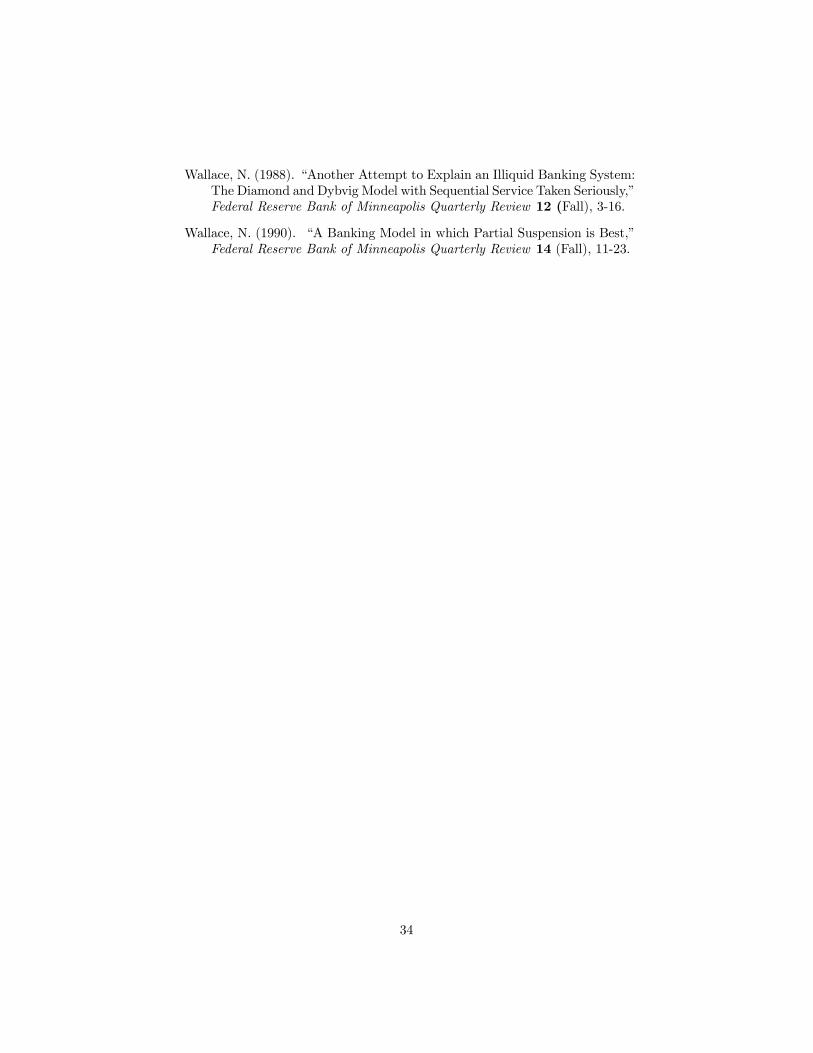
Wallace, N. (1988). �Another Attempt to Explain an Illiquid Banking System:The Diamond and Dybvig Model with Sequential Service Taken Seriously,�Federal Reserve Bank of Minneapolis Quarterly Review 12 (Fall), 3-16.

Wallace, N. (1990). �A Banking Model in which Partial Suspension is Best,�Federal Reserve Bank of Minneapolis Quarterly Review 14 (Fall), 11-23.

34

Table 1Equilibria for Example 1

# ε

·E[Us]E[Ur]

¸ ·ys

yr

¸ (cs1(0), c

s2(0))

(cs1(1), cs2(1))

(cr1(0), cr2(0))

(cr1(1), cr2(1))

·p(0)p(1)

¸1.1A 0 0.081 0.800 (1.000, 1.500) 0.667

1.1B 0

·0.0810.081

¸ ·0.8000

¸ (1.000, 1.500)(1.000, 1.500)(1.414, 1.500)(0.648, 0.648)

·0.9430.432

¸

1.2 0.010

·0.0780.078

¸ ·0.8100.016

¸ (0.998, 1.488)(0.998, 1.520)(1.405, 1.488)(0.651, 0.651)

·0.9400.430

¸

Table 2Equilibria for Example 2

# ε

·E[Us]E[Ur]

¸ ·ys

yr

¸ (cs1(0), c

s2(0))

(cs1(1), cs2(1))

(cr1(0), cr2(0))

(cr1(1), cr2(1))

·p(0)p(1)

¸2.1A 0 0.203 0.500 (1.000, 1.500) 0.667

2.1B 0

·0.2030.111

¸ ·0.5000

¸ (1.000, 1.500)(1.000, 1.500)(1.500, 1.500)(0.563, 0.563)

·1.0000.375

¸

2.2 0.010

·0.1990.110

¸ ·0.5080

¸ (0.996, 1.497)(0.996, 1.507)(1.500, 1.500)(0.561, 0.561)

·1

0.374

¸

35

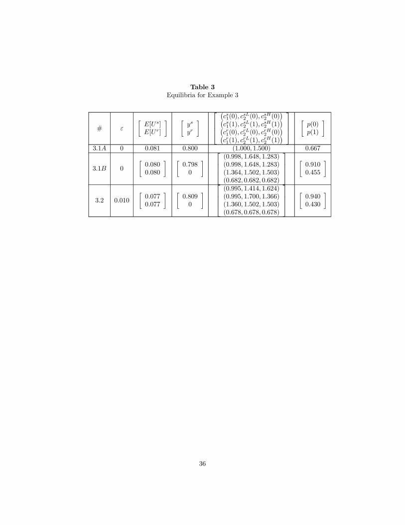
Table 3Equilibria for Example 3

# ε

·E[Us]E[Ur]

¸ ·ys

yr

¸ ¡cs1(0), c

sL2 (0), c

sH2 (0)

¢¡cs1(1), c

sL2 (1), c

sH2 (1)

¢¡cr1(0), c

rL2 (0), c

rH2 (0)

¢¡cr1(1), c

rL2 (1), c

rH2 (1)

¢ ·

p(0)p(1)

¸3.1A 0 0.081 0.800 (1.000, 1.500) 0.667

3.1B 0

·0.0800.080

¸ ·0.7980

¸ (0.998, 1.648, 1.283)(0.998, 1.648, 1.283)(1.364, 1.502, 1.503)(0.682, 0.682, 0.682)

·0.9100.455

¸

3.2 0.010

·0.0770.077

¸ ·0.8090

¸ (0.995, 1.414, 1.624)(0.995, 1.700, 1.366)(1.360, 1.502, 1.503)(0.678, 0.678, 0.678)

·0.9400.430

¸

36

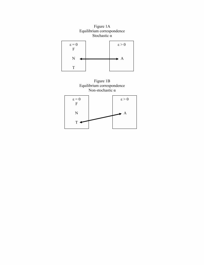
Figure 1A Equilibrium correspondence

Stochastic α

Figure 1B Equilibrium correspondence

Non-stochastic α

ε = 0 F

N

T

ε > 0

A

ε = 0 F

N

T

ε > 0

A