
Final Report: Sustainable Geotechnical Asset...
152
Final Report: Sustainable Geotechnical Asset Management along the Transportation Infrastructure Environment Using Remote Sensing Rüdiger Escobar Wolf, El Hachemi Bouali, Thomas Oommen, Rick Dobson, Stan Vitton, Colin Brooks, and Pasi Lautala Michigan Technological University USDOT Cooperative Agreement No. RITARS-14-H-MTU Principal Investigator: Dr. Thomas Oommen, Assistant Professor Department of Geological and Mining Engineering and Sciences Michigan Technological University 1400 Townsend Drive Houghton, MI 49931 (906) 487-2045 [email protected] Program Manager: Caesar Singh, P.E. Director, University Grants Program/Program Manager OST-Office of the Assistant Secretary for Research and Technology U.S. Dept. of Transportation 1200 New Jersey Avenue, SE, E35-336 Washington, DC 20590 (202) 366-3252 [email protected]
-
Upload
truongquynh -
Category
Documents
-
view
218 -
download
0
Transcript of Final Report: Sustainable Geotechnical Asset...

Final Report: Sustainable Geotechnical Asset Management along the Transportation Infrastructure Environment Using
Remote Sensing
Rüdiger Escobar Wolf, El Hachemi Bouali, Thomas Oommen, Rick Dobson, Stan Vitton, Colin Brooks, and Pasi Lautala
Michigan Technological University USDOT Cooperative Agreement No. RITARS-14-H-MTU
Principal Investigator: Dr. Thomas Oommen, Assistant Professor Department of Geological and Mining Engineering and Sciences Michigan Technological University 1400 Townsend Drive Houghton, MI 49931 (906) 487-2045 [email protected] Program Manager: Caesar Singh, P.E. Director, University Grants Program/Program Manager OST-Office of the Assistant Secretary for Research and Technology U.S. Dept. of Transportation 1200 New Jersey Avenue, SE, E35-336 Washington, DC 20590 (202) 366-3252 [email protected]

2
TABLE OF CONTENTS
Executive summary 8 1: Background 9 1.1 Chapter 1: Background 9 1.2 Current Practices in Asset Management 11 1.3 FHWA Generic Asset Management Framework (FHWA, 1999) 13 1.4 AASHTO Asset Management Plan (AASHTO, 2013) 13 1.5 Risk-based Approach Framework 17 1.6 Bridge Management System 20 1.7 Long-Term Bridge Performance Program 21 1.8 Maintenance Rating Program 22 1.9 Pavement Management Guide 24 1.10 Unstable Slope Management Programs 25 1.11 Oregon DOT-I: Rockfall Hazard Rating System 25 1.12 Asset Management of Embankments – United Kingdom 27 1.13 Limitations of Current Asset Management Plans 28 2. Requirements for Remote Sensing Based Geotechnical Asset Management Systems: Survey on current practices, Perceived Needs and Limitations, by transportation agencies.
34
2.1 Methodology 34 2.2 Results of the survey 35 2.3. Conclusion 40 3: Identification of Remote Sensing Technologies 42 3.1 Introduction 42 3.2 Remote Sensing Techniques 43 3.2.1 Interferometric Synthetic Aperture Radar (InSAR) 43 3.2.2 Light Detection and Ranging (LiDAR) 44 3.2.3 Optical Photogrammetry 45 3.3 Requirements for Remote Sensing Techniques when Applied to GAM: What to Consider Prior to Data Acquisition 46
3.4 Remote Sensing Technologies Rating 48 3.5 Conclusion 50 4: Field verification and evaluation of remote sensing technologies applied to geotechnical asset management 52
4.1. Description of test sites 52 4.1.1 M-10 Highway, Detroit, Michigan 52 4.1.2 Railroad corridor in Nevada 54 4.1.3 Trans Alaska Pipeline corridor 54 4.1.4 Laboratory scaled model setup 55 4.2. Description of the data 56 4.2.1 InSAR datasets 57 4.2.2 LiDAR datasets 59 4.2.3 Photogrammetry datasets 60 4.3. Data processing and results 62 4.3.1 InSAR results for the Nevada test sites 62 4.3.2 InSAR results for the Michigan sites 66

3
4.3.3 InSAR results for the Alaska sites 67 4.3.4 LiDAR results for the Nevada test sites 67 4.3.5 Photogrammetry results for the Nevada test sites 69 4.3.6 Photogrammetry results for the M-10 highway site 70 4.3.7 Photogrammetry results for the Alaska sites 72 4.3.8 Photogrammetry results for the scaled model laboratory tests 73 4.4. Comparison of different methods, limitations and challenges 75 4.5. Conclusions and recommendations 77 5. Performance Monitoring and Condition Assessment 79 5.1 Introduction 79 5.2 Performance Monitoring of Geotechnical Assets 79 5.3 Remote Sensing Techniques for Geotechnical Asset Performance Monitoring and Condition Assessment 83
5.4 The Multi-Tiered Approach 84 5.5 Case Study I: Unstable Slopes along Railroad Corridor in Southeastern Nevada 85 5.6 Case Study II: Retaining Wall on M-10 Highway in Metropolitan Detroit, Michigan 87 5.7 Conclusion 88 6: Geotechnical asset management decision support system 89 6.1. Introduction 89 6.2. Server Software 89 6.3. Client Software 90 6.4. User Interface 91 6.5 Nevada Case Study 92 6.6. Conclusion 95 7 Cost-benefit analysis of remote sensing methods applied to geotechnical asset management 96
7.1. Estimating costs of different technologies and platforms 96 7.2 Satellite based InSAR costs 96 7.3 LiDAR costs 98 7.4 Digital photogrammetry costs 101 7.5. Benefits from each technology and comparison with their costs 103 7.6 Synthesis of costs and benefits 105 7.7. Conclusions 106 8. Remote sensing implementation framework 108 8.1 Using geotechnical asset monitoring information and adopting remote sensing methods for geotechnical asset management 108
8.1.1 Steps to implement a geotechnical asset management system 108 8.1.1.1 Prior work on asset management implementation 108 8.1.1.2 Defining geotechnical asset management system goals and aligning them with the agencies general goals and objectives 109
8.1.1.3 Defining and prioritizing geotechnical assets, and creating and maintain an asset inventory 111
8.1.1.4 Assess and monitor the performance and health for the assets in the inventory 114 8.1.2 Local and regional implementation using GIS visualization and decision support systems 115
8.2 Transportation agencies limitations to adopt remote sensing methods for 115

4
geotechnical asset management, and ways to overcome them 8.3 Example of remote sensing implementation on case study sites, and possible expansions to a complete network 117
8.3.1 Unstable slopes asset management example: Hypothetical case for the Portuguese Bend Landslide Complex (PBLC) on the Palos Verdes Peninsula in California 117
8.3.1.1 Defining geotechnical asset management system goals for the PBLC case, and aligning them with the general goals and objectives of the transportation agency 118
8.3.1.2 Defining and prioritizing geotechnical assets, and creating and maintaining an asset inventory for the PBLC case. 120
8.3.1.3 Assessment and monitor of the performance and health for the assets in the inventory covering the PBLC, using remote sensing methods, and GIS visualization 121
8.3.2 Retaining wall asset management example: Hypothetical case for the M-10 site 125 8.3.2.1 Defining geotechnical asset management system goals for the M-10 Highway case, and aligning them with the general goals and objectives of the transportation agency
125
8.3.2.2 Defining and prioritizing geotechnical assets, and creating and maintaining an asset inventory for the M-10 Highway case 126
8.3.2.3 Assessment and monitor of the performance and health for the assets in the inventory covering the M-10 Highway, using remote sensing methods, and GIS visualization and decision support systems
126
8.4 Conclusions 127 9. Outreach activities 129 9.1 Introduction 129 9.2 Outreach video on remote sensing and geotechnical asset monitoring 129 9.3 Outreach activities with project partners 134 9.4 Conference presentations and publications 136 9.5 Project website 139 References 141

5
GLOSSARY OF TERMS
AASHTO American Association of State Highway and Transportation
ADTT Average Daily Truck Traffic
AEG Association environmental and engineering geologists
ALOS Advanced Land Observing Satellite
ASI Italian Space Agency
Austroads Australian road transport and traffic agencies association
BAM Bridge asset management
BMS Bridge Management System
CCD Charge-Coupled Devices
CD Compact disk
CinOptic Michigan Tech University student media enterprise
COSMO-SkyMed COnstellation of small Satellites for the Mediterranean basin Observation
CSA Canadian Space Agency
DAMA Data Management Association
DEM Digital Elevation Model
DLR German Aerospace Center
DOT Department of Transportation
DSI Distributed Scatterer Interferometry
DSLR Digital single lens reflex
DSS Decision Support System
EAM Embankment asset management
ENVISAT Environmental Satellite from the European Space Agency
ERS Environmental Research Satellite
ESA European Space Agency
FHWA Federal Highway Administration
GAM Geotechnical asset management
GAMDSS Geotechnical asset management decision support system
GIS Geographic Information System
GNSS Global Navigation Satellite Systems

6
GPS Global positioning system
GUI Graphical User Interface
H/L Height to length ratio
HTML Hypertext Markup Language
INS Inertial navigation system
InSAR Interferometric Synthetic Aperture Radar
ISTEA Intermodal Surface Transportation Act
JAXA Japanese Aerospace Exploration Agency
JERS Japanese Earth Resource Satellite
KML Keyhole Markup Language
LiDAR Light Detection and Ranging
LTBP Long-Term Bridge Performance
MDOT Michigan Department of Transportation
MRP Maintenance Rating Program
NBIS National Bridge Inventory System
NCHRP National Cooperative Highway Research Program
NED National Elevation Dataset
OGC Office of Government Commerce
PALSAR Phased Array type L-band Synthetic Aperture Radar
PAM Pavement asset management
PBLC Portuguese Bend Landslide Complex
PMS Pavement Management System
PostgreSQL Object-relational database management system
PSI Persistent Scatterer Interferometry
RADARSAT Canadian Space Agency Earth Observation Satellite
SAM Slope asset management
SAR Synthetic aperture radar
SLC Single look complex
SNR Signal to noise ratio
SqueeSAR™ InSAR processing algorithm by TRE
TAC Technical Advisory Committee

7
TAM Transportation asset management
TerraSAR-X Radar Earth Observation Satellite from the German Aerospace Center
TRB Transportation Research Board
TRE Tele-Rilevamento Europa
USDOT Unites States Department of Transportation
USM Unstable Slope Management
UAV Unmanned Aerial Vehicle
USGS Unites States Geologic Survey
WMS Web Mapping Services
Acknowledgements
This work is supported by the US Department of Transportation, through the Office of the
Assistant Secretary for Research and Technology (USDOT-OST-R). The views, opinions,
findings, and conclusions reflected in this paper are the responsibility of the authors only and do
not represent the official policy or position of the USDOT-OST-R, or any state or other entity.
Additional information regarding this project can be found at www.mtri.org/geoasset.

8
Executive summary
This report summarizes the work and results obtained from USDOT Cooperative Agreement No.
RITARS-14-H-MTU, on remote sensing applications for geotechnical asset management.
Considering the context of transportation asset management, a framework for the application or
remote sensing tools is developed, particularly for monitoring geotechnical asset surface
displacement, as part of the monitoring necessary for geotechnical asset management. A review
of the transportation asset management paradigm is given in chapter 1, and the requirements for
remote sensing based geotechnical asset management are explored in chapter 2. A survey on
current practices, perceived needs and limitations gives an overview of the perspective of
transportation agencies on this topic. Appropriate technologies are identified and selected for the
tasks most relevant to geotechnical asset management, as explained in chapter 3. Field
verification and evaluation of the remote sensing technologies is reported in chapter 4, always
within the context of geotechnical asset monitoring.
The monitoring of geotechnical assets has the goal of continuously or frequently assess the
assets’ performance, according to the transportation management needs. Chapter 5 discusses
asset performance definition and monitoring. Using the geotechnical asset condition information
obtained from the monitoring requires some framework for decision making, the decision
support system discussed in chapter 6 presents a web framework that contribute to this goal. Any
implementation of new technology or methods requires and evaluation of its benefits, weighted
against the costs of adopting such technologies, chapter 7 explores the costs of implementing
remote sensing methods, and the value of the information that can be obtained from them.
For transportation agencies to adopt the new technologies and implementation framework is
necessary. Chapter 8 discusses the implementation framework for the remote sensing
technologies tested in the project, giving also hypothetical examples on two of the field sites
included in the project. The outreach components of the project are summarized in chapter 9,
including the development of an outreach video and the multiple conference presentations and
papers that were generated during the duration of the project.

9
Chapter 1: Background
1.1 Asset Management
The term asset management is defined differently by each individual, government agency, or
corporation, yet essentially means the same thing. In general, any actions implemented to
maintain, preserve, or to perpetuate an asset’s optimal performance level throughout its lifespan
fall under the asset management umbrella. Transportation agencies each have their own official
term. In a report entitled Strategy for improving asset management practices, the Australian road
transport and traffic agencies association (Austroads) defined asset management as “…a
comprehensive and structured approach to the long-term management of assets as tools for the
efficient and effective delivery of community benefits.” (Austroads, 1997). The Federal Highway
Administration (FHWA) expanded on this definition two years later:
“[Asset management is] a systematic approach of maintaining, upgrading, and
operating physical assets cost effectively. It combines engineering principles with
sound business practices and economic theory, and it provides tools to facilitate a
more organized, logical approach to decision making [sic]. Thus, asset
management provides a framework for handling both short- and long-range
planning.” (p8, FHWA, 1999)
Iterations of the asset management definition have been produced since and include portions of
the FHWA definition. For example, the Michigan Department of Transportation (MDOT)
defines asset management as “…a process to strategically manage our transportation system in a
cost-effective and efficient manner” (MDOT, 2015); Flintsch & Bryant, Jr. (2006) define it as
“…a strategic approach to the optimal allocation of resources for the management, operation,
maintenance, and preservation of transportation infrastructure”; the National Cooperative
Highway Research Program (NCHRP) describe a portion of it as “…a strategic and systematic
process of operating, maintaining, upgrading, and expanding physical assets effectively
throughout their life cycle…” (Cambridge Systematics, Inc., et al., 2009). Regardless of the
myriad of definitions and repetitive verbiage, everyone seems to agree that basic asset

10
management requires the maintenance, management, and preservation of all assets along the
transportation corridor.
Although many goals of asset management are included in the definition, the American
Association of State Highway and Transportation (AASHTO) summarized the goals into three
general statements (Cambridge Systematics, Inc. et al., 2002). The first goal is to “build,
preserve, and operate facilities” in a manner that is more “cost-effective” and with an
improvement in “asset performance.” The second goal is to the consumers the “best value for the
public tax dollar spent.” The third goal, which is more political, is to “enhance the credibility and
accountability of the transportation agency to its governing executive and legislative bodies.” Of
these three goals, methodologies towards accomplishing the first two goals have been studied in
great detail, as the third goal is a by-product of the first two.
The United States (US) was relatively late to the asset management game. Asset management
programs were implemented in other countries (Canada, Australia, New Zealand, and across
Europe) in the 1980s and 1990s. The first US-based seminar was held in the Washington, D.C.,
in 1996 with AASHTO and FHWA as hosts. The overwhelming positivity felt from this seminar
lead to successive annual meetings, beginning in 1998 with the Asset Management National
Conference in Scottsdale, Arizona. Then in 2000, the Transportation Research Board (TRB)
joined AASHTO and FHWA to create an “AM [Asset Management] Task Force” (Hawkins &
Smadi, 2013). Since then an increase in research and funding has gone toward many forms of
asset management (e.g., pavement, transportation, bridge, geotechnical, tunnel, etc.) with the US
Department of Transportation (USDOT) and many state DOTs including some sort of asset
management protocol in their annual infrastructure budget. Then on July 6, 2012, law P.L. 112-
141 – the Moving Ahead for Progress in the 21st Century Act (MAP-21) was signed into law
(USDOT, 2015). MAP-21 requires the development of “a risk-based asset management plan for
the National Highway System to improve and preserve the condition of the assets and the
performance of the system” (p1660, Stanley & Pierson, 2013). Transportation asset management
(TAM) is the most widespread asset management plan, with at least 16 states have some sort of
TAM plan currently in place (e.g., Colorado, Connecticut, Florida, Georgia, Indiana, Michigan,
Minnesota, Missouri, Montana, New Jersey, North Carolina, Oregon, Pennsylvania, Utah,

11
Virginia, and Washington – Lindquist & Wendt, 2012). All of these TAM plans include some,
but not all, of other various asset types (e.g., pavement, bridges, geotechnical, tunnels), as other
asset types usually are separated into other management plans. For example, DOTs in
Washington, Oregon, California, and many other western states have a separate rock
fall/landslide hazard program. So basically for those state DOTs with no existing asset
management plan, the most difficult part is how to start; while for those states with existing
TAM plans, the biggest problem is integrating all asset management plans into one system or
network.
1.2 Current Practices in Asset Management
Current practices in asset management vary greatly by transportation agency and again by asset
type. The initial asset management approach was to divide focus by asset type and then create
individual asset management programs. This resulted in the generation of TAM, pavement asset
management (PAM), bridge asset management (BAM), geotechnical asset management (GAM),
slope asset management (SAM), embankment asset management (EAM), and so on and so forth.
The obvious problem with this divide-and-conquer approach is that separate management plans
do not share data or information with any other plan. This can pose a problem since a variety of
assets share the same transportation corridor. For example, one slope failure could potentially
affect assets categorized in all of the management programs listed above. Even worse, some
types of asset management systems do not have standard procedure between states DOTs or
transportation agencies; Vessely (2013) laments that “…there does not appear to be a standard of
practice for geotechnical asset management [GAM] within state and federal transportation
agencies in the United States” (p35). Therefore the need for an integrated asset management
approach is apparent and, according to Anderson & Rivers (2013), recent recommendations have
been made to change the focus from an “asset-by-asset approach to one that examines the entire
corridor.”
Differences by transportation agency and asset type notwithstanding, many DOTs and agencies
have adopted a common asset management approach, which has been dubbed the worst-first
approach. The approach is quite simple: assets that have failed or have degraded to the point of

12
disrepair are either repaired or entirely replaced (FHWA, 1999). There may be two reasons why
a worst-first approach is more common than a preventative approach: (1) tight budgets and
limited funding require addressing the most critical assets, a reactive approach due to safety
concerns, as opposed to spending the money on proactive measures; (2) justification to the
consumers for a proactive and preventative approach is difficult because the tax-payers
essentially expect the assets in the worst condition are addressed first and that, essentially,
preservation is interpreted as “fixing something that isn’t broken” (p21, FHWA, 1999).
In lieu of these reasons, the worst-first approach has been deemed unsustainable. The FHWA
admit that “most states limit application of their management systems to monitoring conditions
and then plan and program their projects on a worst-first basis” and that this approach is “tactical
rather than strategic” (p16, FHWA, 1999). Stanley & Pierson (2013) go one step further and
claim the worst-first approach “results in overall system degradation as no assets receive
preventative maintenance in time to keep the investment optimized” (p1660). So although a
short-term fix of one failed asset may be cheaper, may receive more publicity, and is much easier
to explain to the general public (“It was fixed because it failed!”), it is actually much more
dangerous and, on a longer timeframe, the worst-first approach is more time-consuming and
costly than a preventative approach.
This understanding has led to the creation of many asset management procedures and workflows.
The following sections describe two general asset management workflows (FHWA and
AASHTO) and a risk-based approach framework (Mian et al., 2011) along with a handful of
specific management systems, including: the Bridge Management System, the Long-Term
Bridge Performance Program (FHWA), the Maintenance Rating Program, the Pavement
Management Guide (AASHTO, 2001), a few statewide DOT-based Unstable Slope Management
Programs, and an Asset Management of Embankments program used in the United Kingdom
(Glendinning et al., 2009).

13
1.3 FHWA Generic Asset Management Framework (FHWA, 1999)
The FHWA created a generic asset management framework (Figure 1.1) to illustrate that all asset
management plans should focus on strategy, a preventative approach, as opposed to tactics, a
reactive approach. This flowchart aims to provide the foundation for an asset management
procedure and can be applied on any scale: asset-by-asset, transportation corridor, or entire
network.
Figure 1.1: The seven steps, along with budget allocation, that comprise the generic asset
management framework created by the FHWA (recreated from FHWA, 1999).
Step 1: Goals and Objectives. Goals and objectives, which may take the form of
policies and laws, must first be addressed prior to any actions taken. These goals should align
with realistic expectations for what the asset management program can accomplish. Factors such
as available budget, resources, workforce, and logistics should be examined as potential
limitations and taken into account. The result of Step 1 should include a full understanding of
management goals and objectives, which should in some way reflect the constituents’ needs, and
intended targets should be set for the rest of the generic asset management framework.
Step 2: Asset Inventory. The construction of the asset inventory is a difficult and time-
consuming step. Important questions must be answered before beginning the inventory, such as:
(1) which assets should be included in, and excluded from, the inventory? (2) What information
should be recorded for each asset (e.g., location, value, functions, services, condition, etc.)? (3)
How will the asset information be recorded (e.g., spreadsheet, GIS geodatabase, etc.)? (4) How
will field crews be trained to record subjective information in a consistent manner? The scope of

14
constructing an asset inventory can be daunting, especially when considering scales of entire
transportation networks on the state or federal level. Although initially time-consuming, the
creation of an asset inventory would only need to be completed once and then updated as new
assets are constructed or destroyed and existing assets receive maintenance or upgrades.
Step 3: Condition Assessment. This step aims to identify the condition of each asset and
apply forward modeling to predict asset condition change over time. An initial condition
assessment may have been included in the asset inventory (Step 2). The type of assessment
would vary drastically by asset type – it would not make sense to have the same criteria for
tunnels as for bridges. The current asset condition as well as historical asset condition and
performance assessments are recommended for adequate performance modeling. The goal of this
step is to utilize “analytical tools and reproducible procedures [to] produce viable cost-effective
strategies for allocating budgets to satisfy agency needs and user requirements, using
performance expectations as critical inputs” (p18, FHWA, 1999).
Step 4: Alternative Evaluation. Alternate choices and budget allocations are then
reevaluated if necessary. Any ways to optimize the asset management program should also be
considered. This step is a quality control measure.
Step 5: Maintenance with Short- and Long-Term Plans. Building on what was
accomplished through Steps 2-4, short- and long-term maintenance plans are prepared based on
the information gained. Short-term plans would include reactive measures such as repairing
critically deteriorated assets, replacing assets that have failed, and addressing threats to public
safety or substantial damage to assets in the transportation environment. Long-term plans would
incorporate preventative measures through the use of asset condition assessment criteria (e.g.,
risk-based or hazard-based) that identify assets in need of care via life-cycle monitoring.
Step 6: Program Implementation. This step is pretty basic – the asset management
program now begins. The importance of this step is that, depending on the asset management
program performance, it can either lead back to Step 4, if the program requires additional
optimization, or lead forward to Step 7.
Step 7: Performance Monitoring. The final step of the generic asset management
framework is to assess the performance of the framework which, according to the FHWA, should
be conducted annually. The framework becomes more flexible and dynamic with a repetitive
self-evaluation mindset because external changes, such as varying budget and funding amounts,

15
can be addressed in a timely fashion – or as stated by the FHWA: “…any Asset Management
system should be flexible enough to respond to changes in any of these variables or factors
[policies, goals, asset types and characteristics, budgets, State operating procedures, and business
practices]” (p18, FHWA, 1999).
1.4 AASHTO Asset Management Plan (AASHTO, 2013)
AASHTO has also provided a list of eight components an asset management plan should include:
1. Data Management. As defined by the Data Management Association (DAMA), data
management is “…the development, execution and supervision of plans, policies,
programs and practices that control, protect, deliver and enhance the value of data and
information assets” (p4, DAMA, 2009). Management of data within an asset management
plan would include the organization of data obtained from various technologies (e.g.,
hand-written field notes or data collected from the field in differing formats, asset
pictures, computer spreadsheets, GPS data, etc.) as well as big data storage, access, and
visualization (Vessely, 2013), which may include compiling all data into a geodatabase.
2. Inventory and Condition Surveys. This component is identical to Steps 2 and 3 of the
generic asset management framework (FHWA, 1999). AASHTO (2013) does provide a
list of specific information that should be provided for each asset:
a. Performance Measures
i. Current asset performance rating
ii. Current asset performance with respect to the entire network
iii. Trend analysis (historic asset performance)
iv. Predictive analysis (potential future performance)
b. Geographic Location
c. Jurisdiction Data
d. Functional and Utilization Data
e. Performance Characteristics
f. Construction History and Historical Significance
g. Archive of Valuable Documents

16
3. Levels of Service: which are defined as “…classifications or standards that describe the
quality of service offered to road users, usually by specific facilities or services against
which service performance can be measured” (p21, AASHTO, 2013). Levels of service
are then divided into two groups: (1) customer, how the public interacts with the service,
and (2) technical, what is required by the transportation agency or service provider.
4. Service Life. This is an understanding of how an asset’s performance changes from
deterioration over time. Service life is usually shown in plot-format, with a performance
metric decreasing over time and a comparison between asset preservation and total asset
deterioration (e.g., Figure 1.2).
Figure 1.2: Hypothetical pavement deterioration curve plotting time the pavement condition
index (PCI – y-axis) over time (x-axis). The saw-tooth curve displays the benefits of a
preservation approach compared to the more common worst-first approach, which may lead to
significant deterioration (main curve). Plot was taken from Galehouse et al. (2006).
5. Performance Measures (Outcome Measures) and Condition Indices. Performances
measures quantify the successfulness of the asset management plan; these variables can
also be used as a form of performance quality control. AASHTO’s transportation asset
management plan includes eight performance measure areas: (1) condition, (2) life-cycle
cost, (3) safety, (4) mobility, (5) reliability, (6) customer measures, (7) externalities, and
(8) risk (p16, AASHTO, 2013). Seven performance measures included as goals in MAP-

17
21 are: (1) safety, (2) infrastructure condition, (3) congestion reduction, (4) system
reliability, (5) freight movement and economic vitality, (6) environmental sustainability,
and (7) reduced project delivery delays (USDOT, 2013).
6. Risk Management. Risk is defined as any threat to transportation infrastructure and
operations regardless of cause (AASHTO, 2013). Therefore, risk management is the
practice of identifying, analyzing, and mitigating sources of risk. The generation of a
risk-based approach framework (e.g., see next section – Mian et al., 2011) where the
frequency, likelihood, and/or probability of a risk occurrence is estimated, is the general
goal.
7. Life Cycle and Cost-Benefit Analyses. A life cycle analysis examines the change in asset
performance, cost, deterioration, and potential risk over an asset’s lifespan. A cost-benefit
analysis is a method of calculating the financial pros (benefits) and cons (costs) of a
particular activity or function. In terms of asset management, benefits may include the
savings acquired due to an asset’s performance or the projected savings of asset
preservation instead of total asset failure, while costs may include the actual expense of
asset preservation. The value of an asset is determined by the cost of the asset subtracted
from the benefit of the asset; an asset has positive value if the benefits are greater than the
costs.
8. Decision Support System (DSS). A DSS addresses the following: (1) the needs of an
asset management plan and potential solutions, (2) evaluation of options, and (3) an
analysis of asset performance with respect to investment (AASHTO, 2013).
1.5 Risk-based Approach Framework
The framework for the risk-based approach presented by Mian et al. (2011) could be
incorporated into the Condition Assessment (step 3) and/or Alternative Evaluation (step 4) of the
FHWA generic asset management framework (FHWA, 1999) or the Risk Management step of
the AASHTO Asset Management Plan (AASHTO, 2013). For the purposes of this framework,

18
the definition of ‘risk’ provided by the Office of Government Commerce (OGC) of the United
Kingdom is used, which states:
“Risk is an uncertain event or set of events that, should it occur, will have an
effect on the achievement of objectives. A risk is measured by a combination of
the probability and the magnitude of its impact on objectives.” (OGC, 2007)
The framework consists of five steps (labeled Step 0-4 by Mian et al., 2011) which work to
combine asset management with risk management.
● Step 0: Decision Scope – the scope is clearly defined and should include the following
information:
o Identification of “service aspect and level” (p2, Mian et al., 2011),
o Duration of time the framework will be implemented, and
o Geographic location(s) of assets, transportation corridor, and/or network.
A determination between a proactive approach and a reactive approach must be decided upon as
well. A proactive approach is one where incremental maintenance reduces the probability of
unexpected repairs; a reactive approach, which may be less expensive on the short-term (and
funding can be easier to justify to the public), increases the probability of incidental repairs and
may conflict with performance measures (e.g., life-cycle cost, mobility, and safety - AASHTO,
2013; almost all listed in the MAP-21 guidelines – USDOT, 2013). Basically all asset
management plans strive for a proactive approach.
● Step 1: Hazard Identification – a hazard is any “uncertain event or set of events” that lead
to risk within the transportation environment. Hazards must be identified by:
o Type,
o Magnitude,
o Cause, and
o Impact on service, goals, objectives, and performance measures.

19
● Step 2: Risk Estimation – the calculation of the “likelihood” and “consequence” of the
risk event occurring, which yields a quantifiable output (Mien et al., 2011). Likelihood is
defined as the probability that an event, that has already occurred, would result in a
defined outcome. The consequence is the resultant negative impact, or severity (in
magnitude), from a certain risk. Therefore R=L·C defines the relationship between risk
(R), likelihood (L), and consequence (C) over a period of time (Woodruff, 2005). An
output could be in the form of a risk matrix (Figure 1.3). A risk matrix compares the
likelihood (rows) and consequence/impact (columns) to calculate the risk event level.
Risk matrices can be either qualitative or quantitative, with the latter being the preferred
choice but also requires more data.
Figure 1.3: Example of a qualitative risk matrix (Lee Merkhofer Consulting, 2014).
● Step 3: Risk Evaluation – a two-fold step that defines the maximum risk threshold and
mitigation. The maximum risk threshold is the greatest risk allowable for an asset to be
considered ‘safe’ or not require mitigation. For example, if the maximum risk threshold
were set to ‘Low’ in the risk matrix in Figure 1.3, then all assets with a ‘Moderate,’
‘High,’ or ‘Extreme’ risk would require mitigation actions to be performed. According to
Mien et al. (2011), mitigation may take three forms: “… (1) essential intervention for
critical risks, (2) intervention desirable but not essential, for moderate risks or (3) no
intervention necessary for low risks. The middle category associated with ‘moderate
risks’ is the one that requires the most detailed evaluation and where ‘risk tolerance’ [or

20
maximum risk threshold] becomes an essential part of the decision making” (p4, italics in
original text).
● Step 4: Risk-based Decision Making – finally a decision should be made on what kind of
mitigating action (if any) is required based on many factors, including the risk level, the
assets at risk, the impact on performance measures, etc. The goal of this framework is to
determine an acceptable risk tolerance at a given scale (asset, corridor, and network) and
identify those assets that require further action. Since event risk changes through time,
this framework should be repeated at an interval deemed sufficient for proper asset and
risk management.
1.6 Bridge Management System
The Intermodal Surface Transportation Act (ISTEA) of 1991 required every State DOT to adopt
a Bridge Management System (BMS), which would incorporate (and replace) the National
Bridge Inventory System (NBIS). Included in the NBIS were bridges or culverts greater than 20
feet in length and carried vehicular traffic. Additionally, each bridge was given an initial
condition rating ranging from 0 – failed/closed – to 9 – excellent condition (USDOT, 2005). The
FHWA sponsored the software PONTIS BMS in 1991 and was included in the AASHTO are
software suite in 1995 (FHWA, 1999). PONTIS BMS allowed for the compilation of a detailed
bridge asset inventory, the ability to model various maintenance/repair/mitigation strategies, and
rank assets based on economic criteria (Gutkowski & Arenella, 1998; FHWA 1999).
The BMS and NBIS were good starting points for the further development of bridge and culvert
management. The data collected from these programs would inspire the FHWA to develop the
Long-Term Bridge Performance program, which was launched as a 20-year research program
aimed to “collect, document, maintain, and study high-quality, quantitative performance data on
a representative sample of bridges nationwide” (USDOT, 2012)

21
1.7 Long-Term Bridge Performance Program
The Long-Term Bridge Performance (LTBP) program was created in 2008 after the FHWA
created the NBIS and found that of the more than 600,000 bridges, tunnels, and culverts
inventoried, approximately 151,497 were considered “structurally deficient or functionally
obsolete” (FHWA, 2014). The entire purpose of the LTBP program is to create an inventory
comprised of numerical/quantitative data of bridges across the US; this purpose aligns with the
Asset Inventory (Step 2) and Condition Assessment (Step 3) of the generic asset management
framework (FHWA, 1999) and the Inventory and Condition Surveys step of the Asset
Management Plan (AASHTO, 2013).
The LTBP asset inventory will be compiled through two data collection phases: (1) the
developmental phase and (2) the long-term data collection phase. The developmental phase was
a pilot study conducted on bridges in California, Florida, Minnesota, New Jersey, New York,
Utah, and Virginia. The objective was three-fold: (1) to verify and substantiate the bridge
management data collection procedures, (2) to solidify interests and bonds with state DOTs, and
(3) to make sure enough information is gained to successfully complete the long-term data
collection phase of the project. The long-term data collection phase – which began in March
2013 – is currently ongoing. As of March 2015, two announcements have been released by the
FHWA to update the public on the progress of the second phase. The first announcement,
published June 2013, identified 24 bridges in the Mid-Atlantic region of the US (New Jersey,
Pennsylvania, Delaware, Maryland, and Virginia) that have been selected to be included in initial
field investigations. The second announcement, also published in June 2013, was entitled
Selection Procedure for Reference and Cluster Bridges and includes eight general steps for
bridge selection. The eight steps are as follows (produced here verbatim from FHWA, 2013):
1. Filter all bridges in the selected region using high level criteria.
2. Obtain State prioritization for remaining population.
3. Sort all remaining bridges into “Design of Experiments” subpopulations based on span
length, age and Average Daily Truck Traffic (ADTT).

22
4. Compute the normalized distance measure for each bridge, which defines its
experimental “power.”
5. Rank the bridges within each subpopulation based on the distance measure.
6. Select bridges from each subpopulation based on the distance measure and a set of
supplemental criteria.
7. Examine the distribution of secondary variables.
8. Iterate until a balance distance measure, supplemental criteria, and subpopulation
variability is achieved.
See FHWA (2013) for a complete description of each step. Of particular interest is step 2, which
requires input from the State DOT to prioritize bridges at low, medium, or high status, with high
statuses assigned to the most critical bridges. State DOTs would ideally have an asset
management plan in place (e.g., FHWA, AASHTO, etc.) to quantifiably identify bridges of
highest priority.
1.8 Maintenance Rating Program
The Maintenance Rating Program (MRP), developed in 1985 by the Florida DOT (FDOT), is a
highway asset condition assessment plan on the state level. At least once per year, State DOTs
are tasked with assigning condition ratings to assets along state highway transportation corridors.
Rated corridor elements include (USDOT, 2007):
1. Roadway
2. Roadside
3. Vegetation and Aesthetics
4. Traffic Signs
5. Drainage
The maximum rating for each category is 20 and, therefore, a perfect total rating of 100 is
possible. An 80 was originally set as a passable grade by the FDOT, but since then other states
have had the option to alter their target rating. For example, the North Carolina Turnpike

23
Authority aims for an overall rating of 90/100 for the Triangle Expressway system (NCTA,
2014).
Workers must undergo state-run MRP computer-based training and pass the MRP Handbook
Exam (FDOT, 2013). The goal is to develop a uniform asset rating style from State DOT
employees so that all state’s MRP ratings are consistent, while also dividing up the inventory
rating work into smaller geographic regions.
Unfortunately, to date only six US states (Figure 1.4) and Taiwan (Chou et al., 2006) have (at
least partially) adopted the MRP. Although the MRP may work well at the state-level, the
immediate limitation is the lack of MRP acceptance among many states and, consequently, little
consistency for how assets are rated.
Figure 1.4: US states that have considered the MRP for highway asset condition assessment.
Green-colored states run annual data collections across most, if not all, of their state highway
systems. Yellow-colored states employ the MRP for geographically-limited use (not statewide).
Red-colored states have published a report on the potential benefits of MRP or have expressed
interest in developing an MRP system, but have not executed the program or have instead
constructed a different plan.

24
1.9 Pavement Management Guide
AASHTO released an official definition for Pavement Management System (PMS) in 1993: “A
pavement management system (PMS) is a set of tools or methods that assist decision-makers in
finding optimum strategies for providing, evaluating, and maintaining pavements in a serviceable
condition over a period of time.” (AASHTO, 1993)
In 2001, AASHTO released the Pavement Management Guide, which lists and describes the six
elements required for pavement management (AASHTO, 2001). The six elements are:
1. Asset Inventory. The inventory “…includes information that defines the management
sections and information about the location, limits, size, connectivity to other sections,
number of traffic lanes, route designations, and functional classification for each
management section” (p16, AASHTO, 2001).
2. Condition Assessment. The condition of pavement assets are measured using the
following variables: surface distress, structural capacity, roughness, surface friction, and
skid resistance (AASHTO, 2001; Peterson, 1987).
3. Determination of Needs. Once the basic information has been compiled, a decision must
be made on what work needs to be done (if any) for each pavement asset. Some sort of
hazard rating scale is generally used, such as pavement condition index (PCI), which
assigns a PCI value ranging from 0 to 100 (FHWA, 1991). ‘Trigger values’ are set to
identify the level of maintenance (LOM) required. Default trigger values and LOM are as
follows:
a. 0 ≤ PCI < 25 Heavy Rehabilitation/Reconstruction
b. 25 ≤ PCI < 50 Moderate Rehabilitation
c. 50 ≤ PCI < 75 Light Rehabilitation
d. 75 ≤ PCI ≤ 100 Preventative Maintenance
4. Prioritization of Projects Needing Maintenance and Rehabilitation. Prioritization of
projects to complete is usually based on condition assessment, determination of needs,
available funding, and logistics.

25
5. A Method to Determine the Impact of Funding Decisions. The goal here is to develop
a methodology of determining the most economically efficient implementation of the
program. Every funding agency wants optimal spending of their money.
6. A Feedback Process. Quality measures or a self-assessment rubric to grade the
program’s effectiveness and impact would help in making the pavement management
plan more robust and sustainable.
This pavement management procedure is basically the FHWA’s generic asset management
framework applied to a specific asset type and could be linked to other asset management
procedures in order to create a corridor- or network-wide asset management plan.
1.10 Unstable Slope Management Programs
Unstable Slope Management (USM) programs have been developed by many State DOTs and
aim to identify unstable slopes along transportation corridors before failures occur. These types
of programs incorporate two general asset management steps: asset (slope) inventory and
condition assessment.
The first USM program, implemented by the Oregon DOT (ODOT) and referred to as Oregon
DOT-I or the Rockfall Hazard Rating System, will be described in detail. Other state DOTs have
created their version of the rating system, but since these were based on the original Oregon
DOT-I they will be compared in Table 1.
1.11 Oregon DOT-I: Rockfall Hazard Rating System
The Rockfall Hazard Rating System was created by the ODOT in the 1980s. This system
contains six main features (Pierson, 1991):
1. A uniform method for slope inventory.
2. A preliminary rating of all slopes. Slopes were initially rated based on the estimated
potential for rock on the roadway and historical rock fall activity. In both categories, the
slope would receive an “A” rating if high, “B” rating if moderate, and “C” rating if low.

26
“A” rated slopes then proceed to the detailed rating, while “B” rated slopes will be
addressed if time permits and “C” rated slopes discarded.
3. A detailed rating of all hazardous slopes. The detailed rating would assign a numerical
value, from 1 to 100, to each slope based on the following criteria:
a. Slope height – the vertical height of the slope from which a rock fall is expected
b. Ditch effectiveness – the ability of roadside ditches to restrict falling rocks from
reaching the roadway
c. Average vehicle risk – the percentage of time that a vehicle will be present in the
rock fall hazard zone
d. Percent of decision sight distance – an estimation of the length of roadway, in
feet, a driver must have to make a complex decision, based on vehicle speed, with
respect to the actual length of roadway a driver would have to make the maneuver
e. Roadway width – distance from edge of pavement on one side of the road to the
edge of pavement on the opposite side
f. Geologic character – attempts to describe slope characteristics based on geology
g. Block size or quantity of rock fall per event – a representative estimation of size
and amount of rock fall content per event
h. Climate and presence of water on the slope
i. Rockfall history – chosen from the following options: few falls, occasional falls,
many falls, and constant falls.
A score is assigned to each of the variables listed above. The Rockfall Hazard Rating System
uses only four score options – 3, 9, 27, 81, with greater values indicating more hazardous slopes
– although Pierson claims “…[these score values] are representative scores of a continuum of
points from 1 to 100” (p3, Pierson, 1991).
4. A preliminary design and cost estimate for more serious sections.
5. Project identification and development. Pierson (1991) identifies four ways the results
from the Rockfall Hazard Rating System may be used to determine projects for
construction.
a. Slopes are chosen based on the rating score.

27
b. Slopes are chosen based on the rating score relative to the construction cost.
c. Adjacent slopes that require similar mitigation procedures are grouped together
and chosen based on areal extent.
d. Slopes are chosen based on the rating score and proximity to important
transportation infrastructure.
e. Annual review and update.
Eight other USM plans were constructed based on the Rockfall Hazard Rating System of Pierson
(1991) and ODOT: (1) ODOT-II, an updated version by the Oregon DOT, (2) OHDOT from the
Ohio DOT, (3) NYSDOT from the New York State DOT, (4) UDOT from the Utah DOT, (5)
WSDOT from the Washington State DOT, (6) TDOT from the Tennessee DOT, (7) MODOT
from the Montana DOT, and (8) BCMoT from the British Columbia Ministry of Transportation
(Huang et al. 2009).
1.12 Asset Management of Embankments – United Kingdom (Glendinning et al., 2009)
The embankment management framework described by Glendinning et al. (2009) and Perry et al.
(2003) begin with a risk assessment flowchart (Figure 1.5) and includes a strategic level and a
tactical level. The strategic level examines all the slopes in the transportation network and
includes steps similar to the construction of an asset inventory, slope prioritization based on risk
analysis, maintenance, and asset monitoring. The tactical level focuses on individual slopes and
includes steps such as condition assessment, potential mitigating actions needed, risk analysis,
cost-benefit analysis, and short- and long-term planning.

28
Figure 1.5: Embankment management framework at the strategic and tactical levels
(Glendinning et al., 2009).
Some specifications to the framework were given in Glendinning et al. (2009). Regular
inspections of the assets are performed to assess the current condition of the asset and placed in
an inventory (asset register). Risk analysis is performed by combining the current condition
assessment information with “…historical information in some sort of database… [t]he history
plus the current condition provides information on the possible potential for failure” (p111,
Glendinning et al., 2009) and coupling that information with a risk matrix approach (Figure 1.3)
where “…the consequences of failure including safety and commercial risks… [such as] volume
of traffic, value of the route, diversionary route availability and its strategic importance to the
movement of freight” (p111). Funding and resources are directed where they are most required
and, therefore, maintenance, monitoring, and remediation are performed if and where necessary.
1.13 Limitations of Current Asset Management Plans
Many limitations exist with either (1) the current asset management plans, or (2) implementation
shortcomings of current asset management plans by state or federal DOTs. Below are listed

29
eleven limitations, challenges, or areas within the asset management field that require more
research concentration.
Limitation #1: State-wide inventories are massive.
Steps to collect inventory information on new asset classes, assess the existing condition, and
rate new assets is “…such a large undertaking that… some states (e.g., Colorado and
Washington) recently cut back on plans to inventory and assess retaining walls because of the
cost of implementation and uncertainty in the payoff from the investment” (p11, Anderson &
Rivers, 2013).
Limitation #2: Incomplete inventories.
No state has completed an inventory and initial condition rating for these assets: pavement,
bridges, walls, culverts, slopes, embankments, and drainages (Anderson & Rivers, 2013). State
DOTs have focused on specific asset types based on hazard For example, states in the Western
US (Washington, Oregon, California, and Colorado) focus on rock and soil slope management
due to landslide risks, while states in the Midwest (Michigan, Wisconsin, Ohio, and
Pennsylvania) focus on pavement and bridge management due to deterioration from freeze/thaw
cycles and heavy salt use.
Limitation #3: Different asset types require different methods for measuring condition.
“The expectation of the frequency of [a] rock fall from a rock cut, the long-term settlement of a
bridge approach, movement of an anchored wall, or corrosion of steel reinforcements in
mechanically stabilized earth are all areas in which the profession has not established or has not
developed means for measuring or recording in consistent ways” (p13, Anderson & Rivers,
2013).

30
Limitation #4: Condition variation in time is difficult to predict.
The challenge that has had the least attention “is the need for predicting how performance
changes through time and identification of the most advantageous times for investment for long-
term level or service optimization” (p14, Anderson & Rivers, 2013).
Limitation #5: There exists no good method for predicting large failures from observed
deterioration.
“Someday it will be possible, for example, to identify the deterioration of the [150-ft high side-
hill] embankment on I-75 in Tennessee [which failed in May 2012] and take timely steps to
improve drainage, and thereby the level of service, without such a large negative impact on
performance” (p14, Anderson & Rivers, 2013).
Limitation #6: Geotechnical asset management programs are minimal in scope.
“Many agencies have rock fall management programs that could be classified as geotechnical
asset management efforts; however, the number of programs for other geotechnical features… is
limited” (p24, Vessely, 2013). The author provides a list of possible geotechnical assets that
could be monitored with a comprehensive asset management program: tunnels; retaining walls;
earth retaining structures; embankments; modified native slopes or cut slopes; slopes, both stable
and those displaying deformation, such as rock fall, rockslides, landslides, and even avalanche
sites; road subgrade, rail subgrade, and transportation ground improvements; culverts; quarry and
other material excavation sites.
Limitation #7: Geotechnical asset life-cycle is poorly understood.
Since geotechnical asset management is relatively new compared to other asset management
programs (e.g., pavement, bridges, and highways), the complete life cycle of many geotechnical
assets is not well understood. “There is a general lack of understanding and published data about
the life cycles of most geotechnical assets” (p1659, Stanley & Pierson, 2013).

31
Limitation #8: Future spending estimates are based on present asset deterioration models –
actual spending varies greatly when assets do not deteriorate as projected (asset life-cycle is
poorly understood).
“Current approaches are based on maintaining a balance between the cost of spending now and
spending in the future, versus consequences of failure… In this case [of an embankment failure
that destroyed a rail subgrade], failure to recognize the transient nature of the embankment
behavior has led to increased costs of having to mobilize twice to instigate repair. Historically,
however, there has been very limited information about the future performance of the asset”
(p117, Glendinning et al., 2009).
Limitation #9: The sundry of asset management programs implemented on many levels, by
many agencies/organizations with individual performance measures, results in incompatible
datasets.
“Data integration and sharing for asset management involve bringing in data from various
sources. Most transportation agencies have large quantities of variable, heterogeneous data. Data
heterogeneity usually results from the presence of internal legacy systems that have diverse
structures and formats. The challenge is to create a framework that incorporates all of the data
items needed to perform the desired asset management business functions, addresses the
disparities in data sources and formats, and responds flexibly to changing data requirements
when new business functions are introduced or when existing processes are modified” (p9,
USDOT, 2007).
Limitation #10: Problems experienced by local governments.
According to the Asset Management Overview released by the USDOT (2007), local
governments described nine problems they encountered during the implementation of asset
management programs. The general themes of these problems are listed below:
1. Commitment by management and staff is important.

32
2. Building and maintaining an asset inventory must be accomplished first, but may also be
performed progressively from many sources.
3. Asset condition assessment need not always be performed at the highest sophistication
level to be a valuable decision-making tool.
4. Data formats may range from field notes to spreadsheets to geodatabases.
5. Monitoring of the asset inventory and asset condition assessment is vital in keeping the
asset management program relevant.
6. Decision-making based on the comparison of different asset types can be accomplished
with an asset management program.
7. Asset condition standards are subjective and may vary between local governments,
transportation agencies, and federal agencies and may vary by asset type.
8. Interdepartmental data sharing saves time and money.
9. The simpler the asset management tools, the more likely they will be accepted and widely
used – “the tools need to be easily understandable, adaptable to the user’s specific
interests, and easy to operate without entailing lengthy, tedious activities for data entry,
formatting, and other routine operations” (p19, USDOT, 2007).
Limitation #11: Additional research is needed.
In 2005, a panel discussion focused on research needs and strategies for meeting them. The panel
identified the following research needs (p24, USDOT, 2007):
1. Data collection and integration
a. Maintaining databases of condition data
b. Metadata standards
c. Improving data quality
d. Automated data collection
2. Condition assessment
a. Condition assessment processes for hidden infrastructure
b. Using remote sensing capabilities
c. Better warning systems
d. Linking condition assessment with decision-making processes

33
3. Performance modeling
a. Capturing the effect of routine maintenance in life-value
b. Modeling preventative maintenance
c. Enhanced modeling techniques
d. Defining performance measures
4. Analysis
a. Tradeoffs in the decision-making process
b. Asset valuation methodologies
c. Risk analysis—cost of failure
d. Treatment selection methods
5. Big picture issues
a. Documenting the benefits of asset management
b. Infrastructure security
c. Applications of emerging technologies
d. Sustainable development
6. Teaching infrastructure management
a. Clearinghouse for infrastructure management course materials
b. Translating research into course materials

34
Chapter 2. Requirements for Remote Sensing Based Geotechnical Asset Management
Systems: Survey on current practices, Perceived Needs and Limitations, by transportation
agencies.
The discussion on transportation asset management practices presented in chapter 2 is applicable
to transportation assets in general. In this section we present results from an online survey we
performed amongst transportation agencies, inquiring about current practices, perceived needs
and limitations of geotechnical asset management.
2.1 Methodology
The goal of the survey was to get investigate the current practices, perceived needs and perceived
limitations of geotechnical asset management amongst professionals and practitioners within
transportation agencies. Potential survey respondents were chosen from public contact
information records, mainly via internet pages of transportation agencies, and a few were
contacted through project participant contacts. Email invitations to participate in the survey were
sent to 710 individuals working in transportation agencies in all 50 states of the Union, and a few
professionals working in private railroad companies. A two months period was allowed for
potential participants to fill the survey, after this period 99 individuals had completed all
questions in the survey, and an additional number of participants had partially answered some
parts of the survey. The design, data collection and analysis of the survey followed Federal
Regulations on the use of human subjects in survey studies, and was overseen and approved by
the Michigan Technological University Institutional Review Board.
The survey was designed in an online platform (https://www.surveymonkey.com), for the
respondents’ convenience. The survey is divided in three sections, the first one contains
questions about the respondent’s background, including the agency they work for and their main
job in that agency. The second section asks questions about the current practices involving
geotechnical assets at the respondent’s agency. The third section asks questions about the

35
perceived needs and limitations regarding geotechnical asset managements at their respective
agencies. The actual questions can be seen in the corresponding appendix section.
2.2 Results of the survey
Survey respondents came from a wide geographic distribution, figure 2.1 shows a map of the
number of respondents per state. This sample seems reasonably representative of transportation
agencies nationwide, covering a variety of geographic locations, with different geotechnical
challenges and institutional settings.
Figure 2.1: Survey respondents per state.
A majority of the respondents (72.7%) reported having a geotechnical or geological background,
as show in figure 2.2. This is significant to interpret the rest of answers, as it suggests that they
would be familiar with the importance of geotechnical assets.

36
Figure 2.2: Background of the respondents. Numbers of responses are show in each sector.
Geotechnical asset inventories are a fundamental component of geotechnical asset management
systems, as discussed in chapter 2. Asset inventories were reported for different types of assets
(see figure 2.3), and surprisingly only 13.4% of respondents mentioned that their agencies had no
inventories at all, although another 8.5% did not know if there were any inventories for
geotechnical assets at their agencies.
Figure 2.3: Asset inventories for different asset types. Numbers of responses are show in each
sector.
Having such inventories will facilitate the development of a geotechnical asset management
system for these agencies, and in some cases such a system may already be in the design of
implementation process. The monitoring of assets is crucial for their management, as explained
in chapter 2, and a majority of survey respondents (54.4 %) stated that asset monitoring or

37
intervention was only done when damage or failure was imminent, and only 18.4 % reported
routine inspections of geotechnical assets (see figure 2.4).
Figure 2.4: Reasons given for asset intervention. Numbers of responses are show in each sector.
For those cases in which data are being collected on geotechnical assets (67.1 %) the main data
collection method (33.8 %) is by visual inspection, and only 17.1 % of respondents reported the
collection of some form of deformation data to monitor geotechnical assets (see figure 2.5).
Figure 2.5: Data types collected for each asset. Numbers of responses are show in each sector.
Analyzing the data was done by an engineer or an expert in the majority (68.1 %) of cases, and
only 12.1 % of responses mentioned some form of GIS tool or decision support system for the
analysis of data (see figure 2.6).

38
Figure 2.6: Currently used data analysis methods. Numbers of responses are show in each
sector.
Regarding the perceived needs for geotechnical asset management activities, the priority of data
collection in the near future was heavily focused on visual inspections (35.5 %), although a
significant number of respondents (27.6 %) chose displacement measurements as a priority data
type to be collected in the future (see figure 2.7).
Figure 2.7: Data collection methods seen as the next priority to further develop in the future.
Numbers of responses are show in each sector.
A lack of material or financial resources was the most common (32.6 %) reason chosen by
survey respondents as a current limitation on geotechnical asset monitoring, although a lack of
perceived need was also chosen as a frequent reason (26.3 %) by survey respondents (see figure
2.8).

39
Figure 2.8: Reasons listed as the main limitation to implement geotechnical asset monitoring.
Numbers of responses are show in each sector.
Open ended questions at the end of the survey allowed respondents to express more general
views on the topics covered. Details about the current limitations and how the resources
available have to be prioritized we sometimes expressed by respondents, for instance:
“Geotechnical assets have been not typically been given as much attention as pavements and
structures, perhaps as these works tend to degrade less or have fewer serviceability issues. Most
asset management is linked to high risk or hazard inventories (areas at risk of scour, landslide,
etc.). MnDOT keeps track of the performance (by instrumentation) of critical projects
[centralized], but most 'typical' geotechnical features are monitored by District maintenance
forces.”
Despite limitations in funding, some respondents expressed optimism in developing GAM
capabilities in the near future, for example:
“We have been thwarted in our previous attempts at securing funding for GAM; but there are
indications we may a break-thru soon for our walls inventory & insp.”
Some respondents mentioned ongoing and future GAM components implementation, for
instance:
“Our agency is working on a retaining wall inventory system and planning to incorporate
rockfall inspection and inventory into a more encompassing geohazard management plan that

40
includes performance measures for rockfall, rockslides, landslides, debris flows, sink holes and
embankments.”
Remote sensing was also viewed by some respondents as a potentially useful tool for monitoring
geotechnical assets:
“Remote sensing techniques offer opportunity to monitor geohazard sites much more frequently
and efficiently.”
2.3. Conclusion
The central objective of the survey was to investigate current geotechnical asset management
practices by transportation agencies, as well as their perceived needs and limitations in that topic.
Although many agencies have inventories for some types of geotechnical assets, comprehensive
inventories covering all assets are not common. Existing partial inventories are a first step in the
process of establishing a GAM system, and further efforts need to be built around those
preliminary inventories.
Asset monitoring (e. g. inspection) and maintenance are mainly done in a reactive way, once the
assets are in obvious and urgent need for such evaluations, and possibly repair or replacement.
When data are collected, the most common method is to do a visual inspections, although some
respondents reported that displacement measurements are also done in some cases. Most of the
time the data collected on geotechnical assets are analyzed by an engineer or an expert, and only
in a few cases where GIS tools and decision support systems reported as analysis tools.
Despite this, a majority of respondents mentioned visual observations as the most common
method of data acquisition to be prioritized in the future, but a significant number of respondents
also mentioned displacement measurements as a method to be prioritized in the future. The most
often reported limitations for asset monitoring, where the lack of material and financial
resources, followed by the lack of perceived need.

41
Providing transportation agencies with cost effective methods for data collection and analysis,
may change the current practice and enhance the adoption of asset monitoring methods that are
necessary for geotechnical asset management.

42
Chapter 3: Identification of Remote Sensing Technologies
3.1 Introduction
Transportation asset management (TAM) is a widespread approach for maintaining
transportation infrastructure throughout their life-cycle, from construction and inventory creation
through preservation and failure mitigation (AASHTO, 2011; Cambridge Systematics Inc.,
2002). TAM characteristics may easily be applied to geotechnical assets in the form of
geotechnical asset management (GAM) (Vessely, 2013). Assets included in a full-fledged GAM
program include, but are not limited to, embankments, cut slopes, natural slopes, and earth
retaining walls/structures (Anderson et al., 2008; Stanley & Pierson, 2013).
Similarly, GAM incorporates asset data collection for condition assessments and performance
monitoring. A complete geotechnical site investigation usually requires in situ measurements,
acquisition of material samples, laboratory tests and analyses, site characteristic modeling, and
data interpretation in order to predict the most likely future behavior of each asset. In-depth field-
based data collection and analysis is more expensive and will require a larger workforce. These
financial and temporal requirements apply additional constraints to the limited resources of
transportation agencies and, therefore, complete geotechnical site investigations may not be
performed on a regular basis.
Remote sensing-based methods can provide an intermediate level of information between each
site investigations. Remote sensing allows for higher frequency data collection (greater temporal
resolution) over large areas and usually automated (e.g., acquisition of satellite imagery requires
no work on the part of a transportation agency). The tradeoff is remote sensing data are of lower
spatial resolution, less robust, and are limited by preset geometric viewing angles when
compared to on-foot site investigations. Examples of the application of remote sensing
techniques to GAM programs are numerous, but many do not focus on how obtained products
may be integrated into the GAM framework, mainly with asset condition assessment and long-
term asset monitoring. We propose that surface displacement derived from remotely sensed data
can be used as a quantitative indicator of the life-cycle health of example geotechnical assets.

43
3.2 Remote Sensing Techniques
A brief synopsis of the three remote sensing techniques used in this study (InSAR, LiDAR, and
optical photogrammetry) is given here. For a complete theoretical overview, please refer to
Deliverable 2-A in the Appendix.
3.2.1 Interferometric Synthetic Aperture Radar (InSAR)
InSAR is an active microwave remote sensing technique. There are two basic categories of
InSAR techniques: (1) N-Pass InSAR and (2) InSAR Stacking. N-Pass InSAR uses a small
number of radar images (usually 2-4) while InSAR Stacking utilizes a stack of radar images
(>20); both techniques can be used to monitor ground deformation within the acquisition
timespan (Massonnet et al., 1993; Massonnet et al., 1995). Ground deformation is measured by
calculating the phase change between images. The phase is a physical characteristic of radar
backscatter and can be converted into the change in distance between the sensor and the ground
target, or, in other words, deformation rate of the ground target.
InSAR Stacking is used for the measurement of small ground deformation rates (mm/year-scale)
because, similar to other geophysical methods (e.g., seismic), stacking allows for an increase in
the signal-to-noise ratio (SNR) of the acquired data. One of the two interferometric stacking
techniques used in this study is Persistent Scatterer Interferometry (PSI). The PSI processing
procedure incorporates all of the processing steps described above, but the output differs. This
technique searches the input radar images for pixels with consistently high coherence throughout
a stack of 20 images or more. A pixel with consistent coherence usually exhibits a relatively
stable geometry (no spatial or temporal decorrelation) and a surface that allows for a great
amount of radar backscatter to return to the satellite sensor (echo). Targets that generally fulfill
these requirements are usually anthropogenic structures, such as roads, bridges, buildings, and
dams. They may also be natural features, such as rock outcrops or cliff faces that lack vegetation.
Targets with consistently high radar returns are known as persistent scatterers (PS) and are the
only points with ground displacement information in the PSI output. All other non-PS pixels are

44
discarded and provide no information (Ferretti et al., 2000; Ferretti et al., 2001). The second
interferometric stacking technique used in this study is Distributed Scatterer Interferometry
(DSI). DSI addresses the fourth limitation of PSI (addressed in the previous section), which is
that the PSI technique may yield thousands of PS/kilometer in urban areas, but only tens of
PS/kilometer in rural or vegetated areas. Using DSI, we are able to locate distributed scatterers
(DS) that give us exactly the same information that PS do (e.g., ground velocity), but DSI is
applicable in rural and vegetated regions (Ferretti et al., 2011).
3.2.2 Light Detection and Ranging (LiDAR)
LiDAR is an active remote sensing technique. A light pulse is emitted from a laser sensor,
reflects off an object, and returns back to the sensor to determine the time of flight of the laser
pulse. The time of flight is used to calculate the distance from the sensor to the object. Multiple
datasets acquired at the same location but at different times may be used to calculate changes in
distance; any changes in distance imply movement of the objects being observed. The distance of
the LiDAR sensor from the feature being imaged determines the density and resolution of the
LiDAR data being collected. Close range laser scanning collects dense, high resolution data.
Aircraft mounted LiDAR sensors collect relatively sparse data, but over much larger areas with
great efficiency, compared to static terrestrial LiDAR scanners. As with other remote sensing
technology, LiDAR has seen increases in data collection rates and more dense data sets.
The LiDAR data collected is often described as a point cloud. The point cloud has three-
dimensional position measurements for the features being scanned. Besides the features of
interest on slope, there are other types of data in the point cloud, such as cars on a road, people
on a sidewalk, houses, trees, and even the branches and leaves on a tree. To make the LiDAR
data in the point cloud useful, the data must be processed and filtered. Many LiDAR vendors
provide processing data, however third-party software is usually required for the filtering of data
to derive various LiDAR data products. Filtering airborne data is performed by looking down at
the data from the perspective of the aircraft – and these filtering algorithms were some of the
very first developed to remove features above the ground in order to extract a bare earth data set.
Filtering terrestrial data, from a moving vehicle or a static tripod is more involved because the

45
filtering algorithms are not mature for the various applications that the LiDAR data can be used.
For geotechnical analysis, it is typical to remove vegetation in order to measure the bare earth.
Accuracy and precision of the LiDAR scan data vary with the LiDAR system and its platform.
Distance of the LiDAR scans affects accuracy largely because of the humidity and temperature
of the atmosphere that attenuates and diffracts the laser energy as the laser passes through the air.
Also, the GNSS, and INS referencing affect the accuracy of the LiDAR data. It is important to
note that INS are especially susceptible to a type of error called drift, which adds a cumulative
error until the drift is corrected in a calibration process after the data is collected.
3.2.3 Optical Photogrammetry
Optical photogrammetry is a passive remote sensing technique. Optical remote sensing is most
commonly done by using sensors that are sensitive to the visible portion of the electromagnetic
spectrum. This corresponds to wavelengths of light are between 400 and 700 nm. Optical
systems are able to detect near infrared wavelengths of light (approximately 700 to 1300 nm or
1.3 microns) but use filters to prevent them from being detected by the sensor; however, digital
cameras can have their filter removed. The most common optical sensors are Charge-Coupled
Devices (CCDs), which are used in typical consumer-grade digital cameras. The wide scale
availability of digital cameras and low cost make them a good candidate for characterizing
remote sensing applications. These sensors have been developed to be smaller as they are used
for cell phone cameras as well as in professional photography.
Photogrammetry is “the science or art of deducing the physical dimensions of objects from
measurements on photographs of the objects” (Henriksen, 1994). This includes measurements
made from both film and digital photography. Digital photogrammetry has been demonstrated as
a viable technique for generating 3D models of structures and structural elements (Maas &
Hampel, 2006). In order to perform 3D photogrammetry, the photos need to be taken with at
least a 60% overlap (McGlone et al., 2004). This ensures that a feature on the ground is
represented in at least two photos. At distances closer to the surface than traditional aerial
imagery this technique is more specifically called close-range photogrammetry. Close-range

46
photogrammetry is defined as capturing imagery of an object or the ground from a range of less
than 100 m (328 ft) (Jiang et al., 2008). Typically, 3D models are generated by using the bundle
adjustment principle (Triggs et al., 2000). This process used determines the orientation of each
image in a series of overlapping images to generate a sparse point cloud (Triggs et al., 2000).
This process allows for images to be taken at different angles, which occurs when the camera
rolls and changes pitch as it is moved across its target.
3.3 Requirements for Remote Sensing Techniques when Applied to GAM: What to
Consider Prior to Data Acquisition
There are many site-specific considerations required for optimal use of InSAR, LiDAR, and
optical photogrammetry. Each remote sensing technique has its advantages and limitations; these
must be acknowledged and understood prior to data analysis, or the user may be surprised by the
results. An in-depth discussion of all considerations is not discussed here – that may be found in
the literature. Instead, a concise list of general requirements for each technique is listed below.
InSAR
1. PS/DS point locations are unknown prior to processing. Due to the slant-range nature of
synthetic aperture radar acquisition, there is a possibility that some geotechnical assets
will not be observed by the radar sensor (this is especially the case in mountainous
terrain). Therefore, unfortunately, PSI and DSI will be unable to measure ground
deformation on these geotechnical assets.
2. Topography and satellite view angle will dictate the number of geotechnical assets visible
and analyzable. The shadow effect, where areas of topographic high will block a satellite
sensor’s view of lower topography behind the peak, is common in mountainous terrain
and results in areas of data loss. Shadow zones can be located, but no data is retrievable.
3. The geometry of the geotechnical asset with respect to the satellite view direction dictates
how much of the asset, if any at all, is viewable from the sensor. Ideally a geotechnical
asset will be in the direct line-of-sight of the radar sensor (single reflection) or in a
geometrically advantageous position where the sensor can view the asset through
multiple bounces (multiple reflections).

47
4. The amount and type of vegetation impacts the number of PS/DS points available on
and/or around a geotechnical asset. Coherence is inversely proportional to the amount
and density of vegetation, with high amounts of vegetation and/or dense (thick)
vegetation resulting in a low coherence, which means a lower likelihood of PS/DS points
occurring in that area.
5. If the ground motion exceeds one-half the radar wavelength between each acquisition, the
geotechnical asset will decorrelate and no information can be gained. Ways to avoid this
problem are to (1) acquire enough radar images close together temporally, (2) process
imagery from longer wavelength sensors, or (3) avoid trying to monitor geotechnical
assets with relatively high displacement rates.
6. Although radar penetrates clouds, it is affected by variations in moisture content in both
the atmosphere and on/in the ground. The best conditions for radar acquisition are when
there is low atmospheric variability and moisture content and the ground moisture content
is consistent at each acquisition date.
7. Depending on the size of the geotechnical asset network (area of interest), multiple stacks
of radar imagery (with 20+ images per stack) may be required for PSI/DSI processing.
8. Image coverage varies throughout the world because the space agencies have different
areas of interest. Check online catalogs from respective space agencies to see spatial and
temporal coverage.
LiDAR
1. Mobile LiDAR is much more efficient at acquiring data on the regional scale, compared
to terrestrial LiDAR which works well at the site-by-site level. Terrestrial LiDAR is
superior in data density and accuracy, but mobile LiDAR allows for a cheaper and
quicker method of acquiring data over large areas.
2. Mobile LiDAR (e.g., airborne or ground vehicle) require precise synchronization and
calibration with GNSS and INS systems. This will reduce position and orientation error
caused by INS drift, which is increases with longer survey times. Both horizontal and
vertical controls are also required so that the resultant point cloud is projected in a proper
coordinate system using an ellipsoid datum.

48
3. It is difficult to differentiate small-scale features, whether they be geotechnical,
geological, or hazard related.
4. Repeated surveys with established ground control can be used to generate in-depth
analysis of geotechnical hazards and risks across observable assets. Multiple acquisitions
can be used to monitor changes in deformation rates, asset location, asset shape, and
other hazardous changes such as erosion, scouring, or weathering.
5. Terrestrial LiDAR surveys are limited to the sensor view angles and, since repeat surveys
require the LiDAR to occupy the same position each time, shadow zones will never be
visible.
Optical Photogrammetry
1. Aerial optical photogrammetry – imagery acquired using satellite, airplane, or unmanned
aerial vehicle (UAV) – allow for the rapid assessment of geotechnical assets over a large
area.
2. Since this is a passive technique, optical imagery can only be acquired during the day
and, using aerial vehicles, when there is no cloud cover. Other obvious obstructions, such
as snow or vegetation, will also lessen the effectiveness of optical photogrammetry. The
time of day is also critical, as lighting variations could introduce glare in the optical
image which will affect processing results.
3. Weather remains the largest factor of successful data collection for aerial vehicles,
especially for UAVs which are easily affected by turbulence and adverse weather
conditions (e.g., precipitation).
4. Resolution is directly proportional to the distance from the asset. A higher resolution
results in less coverage, and vice versa.
3.4 Remote Sensing Technologies Rating
A relative rating to compare the effectiveness of InSAR, LiDAR, and optical photogrammetry
was performed using the method suggested by Ahlborn et al. (2010). The rating is based on the
perceived performance with respect to GAM of these three techniques. A series of performance
criteria were defined and a score for each criterion was chosen based on the evaluation method,

49
with a score of 1 meaning least adequate at meeting the criterion and 3 meaning the method fully
meets the criterion. Seven criteria were selected based on a GAM literature review (Anderson et
al., 2008; Stanley et al., 2013; Vessely, 2013). The criteria are:
1. Information Content. How relevant is the information gained from each technique
towards GAM?
2. Spatial Density and Ground Resolution. How many data points are acquired over one
image pixel?
3. Data Availability and Revisit Time. How many images are available and how often are
images acquired?
4. Accuracy. How do the data acquired by remote sensing techniques compare to in situ
and field measurements (ground-truthing)?
5. Direct Cost for Data Collection and Analysis. How much does it cost to acquire,
process, analyze, and interpret the data collected by the remote sensing technique?
6. Indirect Cost for Data Collection and Analysis. How much does it cost to purchase the
instruments and train staff to acquire data?
7. Availability of Historical Data. How far into the past are relevant data available and
usable for the technique?
Table 1 shows the results of the remote sensing technologies rating. InSAR outperforms the
other techniques with respect to the direct cost for data collection and analysis (which, for
educational purposes, can be free with acceptance of a proposal) and availability of historical
data. Optical photogrammetry outperforms the other techniques with respect to the indirect cost
for data collection and analysis. LiDAR, although not outperforming all other techniques in any
one given category, posts solid scores in four of the seven categories, including the data’s spatial
density/ground resolution and data availability and revisit time.

50
Table 3.1: Performance ratings
Criteria
InSAR LiDAR
Optical
Photogrammetr
y
Information Content 3 3 3
Spatial Density and Ground Resolution 2 3 3
Data Availability and Revisit Time 2 3 3
Accuracy 3 3 3
Direct Cost for Data Collection and
Analysis 3 2 2
Indirect Cost for Data Collection and
Analysis 3 1 3
Availability of Historical Data 3 1 2
3.5 Conclusion
Geotechnical assets, such as retaining walls, embankments, cut slopes, and rock slopes are
indispensable components for healthy transportation infrastructure. According to the American
Association of State Highway and Transportations Officials’ (AASHTO) Transportation Asset
Management Guide, over the past decade there has been a growing awareness that the current
methods of transportation infrastructure management are not adequate to meet the demands of
the public and therefore, need improvement (AASHTO 2013).
Current practices for managing geotechnical assets along transportation corridors are mostly
focused on restoring the asset after failure, as opposed to identifying and remediating hazardous
conditions before their occurrence. One of the reasons for lacking a proactive system is,
geotechnical assets are extensive and assessing their condition using traditional site inspection is
mostly qualitative and laborious.
The applicability of three remote sensing techniques (InSAR, LiDAR, and Photogrammetry)
were rated for geotechnical asset management based on different criteria. Results indicate that

51
there is no technique that has high rating for all criteria. In general, the photogrammetry method
is the most cost effective and easy to process, whereas, the InSAR method has the relatively low
cost per km2 and can provide mm scale accuracy. The LiDAR and photogrammetry are
comparable except that the initial cost for LiDAR instrumentation can be significantly higher.
The detailed rating results presented in Table 1 highlight the criteria of the remote sensing
techniques that have potential to impact the current practices for geotechnical asset management,
and also the ones that need additional sensor development and commercialization. Ongoing and
future activities of this study will investigate the field performance of these remote sensing
techniques for geotechnical asset management.

52
Chapter 4: Field verification and evaluation of remote sensing technologies applied to
geotechnical asset management
The different remote sensing technologies identified to have potential for monitoring and
assessment purposes within a geotechnical asset management system, as described in chapter 4,
were tested for performance and applicability to specific asset management tasks. The ability to
use remote sensing to measure surface deformation over time was particularly relevant for such
technologies. This chapter summarizes the extensive field verification and evaluation of the
remote sensing technologies, as applicable to different geotechnical asset monitoring scenarios.
4.1. Description of test sites
Field and laboratory test sites were chosen at different locations, and included a variety of
geotechnical asset types, including retaining walls, and natural and artificial slopes in rock, soil
and permafrost environments. Three different field locations in Michigan, Nevada and Alaska
were chosen for field site testing. Assets were located in different types of transportation
corridors, including highways, railroads and pipelines. Laboratory testing on scaled models of
retaining walls was also performed.
4.1.1 M-10 Highway, Detroit, Michigan
A series of retaining walls on M-10 highway in Detroit, Michigan, were chosen to test remote
sensing methods for surface displacement measurements. The retaining walls were near the
junction between the M-10 highway and Meyers Road (see figure 4.1). At the test location the
M-10 is a depressed highway with three traffic lanes in in each direction, confined by 16 feet tall,
vertical cantilever retaining walls, separated in 100 feet sections. Parallel running service drives
are located on top the fill behind the retaining walls. Retaining wall sections move independently
in response to stresses.

53
Figure 4.1. Upper panel, location of the retaining walls along M-10 highway, Detroit, Michigan.
(Taken from Cerminaro, 2014). Lower panel, picture of the retaining walls.
The retaining walls were designed and build in the 1950’s and 1960’s, using tension tie-backs to
increase wall stability to overturning and reduce wall footing size (Jasson, 2013). In the original
design the tie-backs were specified as cables but were changed to solid bars in the actual
construction, and this change, coupled with back-all drainage problems is believed to have led to
the wall failure (Cerminaro, 2014). Significant movement between retaining wall sections, up to
8 cm, was observed at the site, leading to the replacement of some sections.

54
4.1.2 Railroad corridor in Nevada
A railroad corridor section of approximately 30 km in Nevada was chosen as test site for
monitoring surface movement on rock slopes. This site included several known rock slide
locations, which had shown significant slope movement in recent times. The railroad corridor is
located within a series of steep sided canyons throughout most of the 30 km stretch, with rock
slopes composed of old volcanic materials. Bouali et al. (2016a) give a detailed description of
this site.
A regional scale analysis of the 30 km railroad corridor focused on methods to identify potential
unstable slopes at a large scale. At a local scale, a few particular slopes were examined in more
detail, using remote sensing methods that would only be applicable at smaller scale targets.
Figure 4.2 shows some of the rock slopes chosen to test such remote sensing methods.
Figure 4.2 – Slopes chosen to perform detailed work due to large displacements and
instabilities.
4.1.3 Trans Alaska Pipeline corridor
The Trans-Alaska Pipeline System was targeted for selection of field testing sites, particularly at
steep slopes on permafrost soil (see figure 4.3). Out of six initial sites identified for potential
fieldwork, two locations, Treasure Creek and Lost Creek, were chosen for in-depth analysis of

55
slope movement measurements using remote sensing methods. An additional site near the
highway (and pipeline) bridge over the Yukon River was also added for in-depth analysis later
on, despite the availability of ground control points.
Treasure Creek and Lost Creek are located on steep permafrost slopes, exceeding 20º in some
places, and have recently shown significant movements, in excess of 1 m at some locations.
Slumping, cracking and other surface deformation features at the sites were observed during
fieldwork, reflecting such significant movements.
Figure 4.3. Treasure Creek pipeline section in Alaska. Left panel shows the view down a steep
slope along the pipeline. Right panel shows the same area as seen I the left panel, but
reconstructed from the photogrammetric point cloud.
4.1.4 Laboratory scaled model setup
Controlled tests in a laboratory setting were also performed on scaled models of retaining walls.
A model setup which mimicked two adjacent retaining wall sections that presented differential
movement was designed and build out of wood and Styrofoam (see figure 4.4). Two boards, 8

56
feet tall by 4 feet wide were mounted on hinges to allow vertical tilting, simulating retaining wall
rotation. Board sections are mounted on independent structures which allows any type of
differential movement between both sections to be modeled. The system is mounted on wheels
and can be displayed indoors and outdoors, to simulate different lighting conditions. Different
texturing types of the Styrofoam boards was also included in the experimental setup.
Figure 4.4. Scaled models build to represent retaining wall movements in the laboratory.
4.2. Description of the data
Datasets analyzed in this project include data collected during its execution, but also data
collected previously by project partners or other agencies. InSAR and LiDAR datasets spanning
several years were analyzed, and additional LiDAR and photogrammetric data were collected
during the project. Here we summarize these datasets, and refer to reader to the appendices for
more detailed information.

57
4.2.1 InSAR datasets
We used moderate ground resolution InSAR satellite data (30 m) and wavelength (C Band - 5.6
cm), and table 5.1 summarizes the different types of available datasets. Of all the available
datasets listed on table 5.1, only subsets from a few were employed in the analysis, as will be
described in the corresponding section. Datasets were chosen to allow for the use of staking
techniques like PSI, as this allowed for points in relatively low coherence areas to be analyzed,
as discussed in the results section.
Table 4.1 List of historical, present, and future InSAR-compatible satellites.
Satellite Mission Timespan
Revisit Period (days)
Ground Resolution (meters)
Radar Band*
Organization Price Per Image (US Dollars)**
Commercial
Research
ERS-1 1991 - 2000
35 25 C European Space Agency (ESA)
$212 - $354 FREE
JERS-1 1992 - 1998
44 18 L Japan Aerospace Exploration
Agency (JAXA)
FREE (limited)
ERS-2 1995 - 2011
35 25 C ESA $212 - $354 FREE
RADARSAT-1
1995 - 2013
24 10-100 C Canadian Space Agency (CSA)
$3,047 - $3809
FREE
ENVISAT 2002 - 2013
35 25-150 C ESA $354 - $591 FREE
ALOS PALSAR
2006 - 2011
46 7-100 L JAXA $42 - $709 FREE
RADARSAT-2
2007 - 24 3-100 C CSA $3,047 - $7,110
COSMO-SkyMed
2007 - 16 1-100 X Italian Space Agency (ASI)
$680 - $2,268
TerraSAR-X 2007 - 11 1-16 X German Aerospace Center
(DLR)
$875 - $7,972
TecSAR 2008 - 14 1-8 X Israel Aerospace Industries
NA
Meteor-3M 2009 - 3 400-1,000 X RosHydroMet $30/$40 - ? RISAT-2 2009 - 14 1-8 X Indian Space NA (contact Antrix)

58
Research Organization
(ISRO) TanDEM-X 2010 - 11 1-16 X DLR NA $118 RISAT-1 2012 - 25 1-50 C ISRO NA (contact Antrix) HJ-1C 2012 - 1 20 S NDRCC/SEPA of
China NA
KOMPSAT-5 2013 - 28 1-20 X Korean Aerospace Research Institute
(KARI)
NA
ALOS PALSAR-2
2014 - 14 1-100 L JAXA $1,257 - $4,191
FREE
Kondor-E1 2014 - 2-3 1-30 S NPO Mashinostroyenia
NA
Sentinel-1A 2014 - 12 4-80 C ESA FREE KOMPSAT-7 2014 - 14 1-20 X KARI NA SAOCOM Constellation
2015 - 8-16 10-100 L Comisión Nacional de Actividades Espaciales
SEOSAR/Paz 2015 - 11 1-15 X Satélite Español de Observación
SAR
Will be publically available
Sentinal-1B 2016 - 6 4-80 C ESA Will be FREE COSMO-SkyMed 2nd Generation
2016 - 1.5-10 1-35 X ASI Will be publically available
TerraSAR-NG
2017 - ~0.42 0.25-30 X DLR
RadarSat Constellation
2018 - 3-12 3-100 C CSA
RISAT-1A 2019 - 12 1-50 C ISRO BIOMASS 2020 - 25 50-60 P ESA NISAR 2020 - L, S NASA & ISRO DESDynI ? - 10 L NASA
SCLP ? - X, Ku
NASA
*P Band (� = 69 cm); L Band (� = 23.6 cm); S Band (� = 9.6 cm); C Band (� = 5.6 cm); X Band (� = 3.1 cm); Ku Band (� = 2 cm) **US Dollar exchange rates (January 2015). NA = not available for commercial/educational use. Prices and data availability listed for users in the United States.

59
4.2.2 LiDAR datasets
Aerial and terrestrial (static) LiDAR datasets were used for this project. Aerial LiDAR data
include publicly available datasets for the Michigan and Alaska sites, as well as aerial dataset
collected and made available to us by project partners. Terrestrial LiDAR datasets collected prior
to the project at the Nevada site were also made available to us (see figure 4.5), and additional
terrestrial LiDAR data were collected for that site during the project. Terrestrial LiDAR data
were also collected for the laboratory setup, to compare the results with the photogrammetric
methods.
Figure 4.5. LiDAR acquisition dates for datasets obtained prior to the project at the Nevada
testing site.
Aerial datasets typically have point densities of less than 10 points per m2 and the associated
errors are of the order of tens of centimeters. Due to its relatively lower resolution and precision,
aerial LiDAR datasets were mainly used for ancillary data purposes (e. g. generation of high
resolution DEMs, etc.) that are also necessary for the transportation asset management (Escobar-
Wolf et al., 2015, Justice, 2015).
Terrestrial LiDAR datasets have much higher point densities, up to thousands of points per m2
(see figure 4.6), and much higher precision, typically on the order of 1 to 2 cm. Terrestrial
LiDAR dataset used for the Nevada site include 11 point clouds acquired between 2011 and
2014 (see figure 4.5), provided by one of the project partners.

60
Figure 4.6. Surface point densities for a rock slope at the Nevada test site.
4.2.3 Photogrammetry datasets
Photogrammetric datasets (i. e. photographs) were acquired at all field testing sites. Table 5.2
summarizes the photogrammetric datasets collected during the project. Photographs were taken
from different platforms, including terrestrial (static and mobile) and aerial (from UAVs and
helicopter). Cameras used include DSLR high resolution (16 to 36 megapixel) cameras, with 35
to 55 mm optical lenses, and data acquisition plans were designed to maximize photographic
overlap and redundancy. A cinematographic camera was also used to test high speed terrestrial
mobile data acquisition.

61
Table 4.2. List of field sites where digital photogrammetric data were acquired between 2014
and 2015. The platform for the data acquisition is also indicated.
Site or location 2014 field work 2015 field work
Helicopter
or UAV
Terrestrial Mobile Helicopter
or UAV
Terrestrial Mobile
Treasure Creek, Alaska x x x x x x
Lost Creek, Alaska x x x x
Dalton Highway landslide
site, Alaska
x x
Dalton Highway Yukon
Bridge, Alaska
x x
Delta Bridge, Alaska x
Glitter Gulch, Alaska x x x x x
Nevada test site, location 1 x x x x x x
Nevada test site, location 2 x x
Hill Street, Cincinnati,
Ohio
x x x x x x
Elboran Street, Cincinnati,
Ohio
x x x x x x
Laboratory scaled model
setup
x x
Michigan Tech Campus
walls
x
Photogrammetry data acquisition was done in the field in 2014 and 2015 at the Michigan,
Nevada, and Alaska sites, using aerial (UAV’s and helicopter) and terrestrial (static and mobile)
platforms. Ground control was either provided by project research partners or collected in the
field and laboratory experiments, using either a Trimble GeoExplorer GNSS receiver or a total
station. Ground control precision estimates put errors at < 10 cm for the GPS surveyed points,

62
and < 3 mm for the total station surveyed ground control. Ground control precision for data
provided by research partners varies but is assumed to be similar to that of the total station.
4.3. Data processing and results
Data processing was focused on measuring surface displacement values of potentially unstable
retaining walls and slopes, but additional useful information for the geotechnical asset
management process was also extracted in some cases, e. g. high resolution DEMs.
Displacement measurements were done by comparing spatial data acquired at different times,
such comparison can be between the locations of points at the surface. In the case of LiDAR and
photogrammetry the displacement measurement can be done by subtracting the location vector of
common points, between datasets acquired at different times. In the case of InSAR this is done
by means of interferometry, i. e. by comparing the phase of radar waves reflected by the target
surface.
Point datasets, as those provided by photogrammetry, LiDAR and InSAR, are unavoidably
incomplete representations of continuous surfaces, and the locations of points in three-
dimensional space are also subject to errors. Assessing how well such point clouds represent the
real surface, and quantifying the associated errors is crucial, especially when we aim to detect cm
to sub-cm magnitude displacements of such surfaces. For these reasons, point surface densities
and point location errors estimations are required to assess the quality of the datasets (Sahoo et
al. 2007; Shan and Toth, 2008).
4.3.1 InSAR results for the Nevada test sites
Ninety radar images acquired between August 20, 1992 and August 15, 2010 over the Nevada
test site were used in the InSAR analysis, 40 from ERS-1 and ERS-2 satellites and 50 from
ENVISAT, corresponding to C-Band SAR antennae sensors operating at a 5.331 GHz frequency.
Images had a descending track line-of-sight (LOS) with an azimuth direction of N86°W, and an
incidence angle centered at 23º from nadir. Data processing was done using a PSI algorithm
within the ENVI SARscape software, and SqueeSAR™ algorithm processing was done by TRE

63
Canada, following the algorithms developed by Tele-Rilevamento Europa (TRE), in a joint PSI-
DSI processing. All measurements presented are positive (towards the satellite) and negative
(away from the satellite) displacements along the satellite-ground line of site at the time of image
acquisition.
Figure 4.7a shows PSI results for the Nevada test site. High coherence thresholds, slope
geometry and vegetation reduced the number of PS points, but overall the PS results agree with
ground observations, showing larger movements in areas where slope instability was observed in
the field. Surface displacement velocities were as high as -2.57 mm/year for the unstable block,
while smaller velocities of -0.97 mm/year were measured upslope from the unstable block, and
can be contrasted with virtually stable terrain to the north (-0.43 mm/year) and south (-0.97
mm/year). Areas potentially affected by runoff exhibited abnormally high velocities (Runoff A: -
3.50 mm/year; Runoff B: -0.86 mm/year in figure 4.7b).
Results from the SqueeSAR™ algorithm (Ferretti et al., 2011) are shown in figure 4.8, and it
becomes apparent that this technique is able to resolve surface displacement for more points. The
SqueeSAR™ results show a general agreement with the PSI displacement measurements, with
the largest displacements confined to the same unstable block as identified in the PSI results, and
smaller displacements measured in the more stable, adjacent terrain.

64
Figure 4.7 Displacements obtained from InSAR analysis for the Nevada test site. (a) Results
from PSI analysis. (b) Segmentation of areas with similar displacement values. The red polygon
shows the slope with the highest displacement values. The orange polygon corresponds to
intermediate velocities, and the green areas show stable (within the error margins) areas

65
Figure 4.8 Results from applying the SqueeSAR™ results to the same slopes shown in figure 4.7.
Time series plots of displacement from DS point on the unstable slope show surface movement
beginning in 2005 (see figure 4.9), and an apparent previous period of stability going back to
1992. These results are consistent with geotechnical reports and persona communications with
the railroad company technicians.

66
Figure 4.9 Time-series of measured displacement for the highly unstable slope shown in figures
4.7 and 4.8, for the three DS points.
4.3.2 InSAR results for the Michigan sites
InSAR results for the Detroit area test site in Michigan were less successful in showing surface
displacement for the retaining walls initially targeted in the project, however other nearby areas
did show interesting surface displacement patterns. PSI InSAR analysis of SAR images covering
the entire Detroit metropolitan area was accomplished with 50 ERS-1/-2 SAR images covering
the 1992 to 2000 period, and revealed a maximum subsidence velocity of 4.2 mm/year and a
maximum uplift of 4.0 mm/year for particular pixels in the area (see figure 4.10).

67
Figure 4.10 Results from PSI processing for the metropolitan Detroit area.
4.3.3 InSAR results for the Alaska sites
Results from InSAR processing for the Alaska sites were mostly unsuccessful (Bouali et al.,
2014), with individual interferograms showings low coherence values and even preventing the
use of staking techniques. The general low coherence is likely the result of extensive forest
coverage and the lack of suitable persistent reflectors along the pipeline corridor.
4.3.4 LiDAR results for the Nevada test sites
Surface displacements measurements derived from comparing 11 LiDAR datasets acquired
between 2011 and 2014 on the unstable rock slope in the Nevada test site, clearly show that
significant displacement took period on that slope during the covered time period. Figure 4.11
shows vertical cross sections generated perpendicularly to the rock slope, from LiDAR point
clouds acquired at different times, and the outwards slope movement is evident.

68
Figure 4.11. Vertical profiles derived from LiDAR data for the Nevada test site. Surface
displacements between June and November 2011 are obvious.
Maps showing displacements perpendicular to the main slope plane were also generated through
DEM differences, projected on a plane parallel to the main slope plane. Displacements of more
than 50 cm were observed for significant portions of the slope, and the movement of large (> 2 m
diameter) individual rock blocks, possibly related to rockfall, also became evident, as can be
seen in figure 4.12.

69
Figure 4.12. Surface changes perpendicular to the unstable rock slope at the Nevada test site,
derived from LiDAR data. Large voids (blue patches) correspond to rockfall events, deposition
areas (red triangular areas) correspond to depositional debris fans at the foot of the slopes, and
relatively small displacements over broad areas (large yellow areas) correspond to actual slope
displacements of large sliding blocks.
4.3.5 Photogrammetry results for the Nevada test sites
Digital photogrammetric results for the Nevada test sites were used to generate high resolution
DEMs and orthophotos (see figure 4.13), but problems with georeferencing and scaling of the
models prevented us from getting high precision DEMs, making it impossible to measure small
surface displacements. Photographs acquired from an aerial (UAV) platform were processed, in
conjunction with rapid GPS (Trimble GeoExplorer GNSS) surveyed control points. Despite high
surface point densities (> 1000 points per m2), overall scaling differences on the order of 1 to 2
%, which amount to > 1 m errors over the > 100 m extent of the datasets, precluded us from
confidently resolving surface displacements of less than the potential errors (i. e. displacements <
1 m). The low precision of the point clouds could be linked to the use of a quick GPS
georeferencing for the control points, but other factors cannot be excluded. Digital
photogrammetric processing was done using the Photoscan (Agisoft, 2016) software.

70
Figure 4.13. Orthophotographs (left) and corresponding hillshade map (right) derived from a
high resolution DEM produced from digital photogrammetry at the Nevada test site.
4.3.6 Photogrammetry results for the M-10 highway site
Surface displacement measurements using digital photogrammetry gave very encouraging results
for the M-10 highway retaining walls site, in Detroit, Michigan. Point clouds derived from the
digital photogrammetry were collected in the spring and fall of 2014, had high surface point
densities (> 1000 points per m2), and were used to estimate surface displacements perpendicular
to the retaining wall plane. Digital photogrammetric processing was done using the Photoscan
(Agisoft, 2016) software.
Figure 4.14 shows a map of the surface displacement perpendicular to the wall plane between
two data acquisition campaigns in March and June of 2014. Displacement measurements of
individual points can be improved upon by considering larger sets of points and assuming rigid
displacement of the wall sections, to reduce the noise associated with random variability of pixel
positions. Figure 4.15 shows the distribution of residuals around the mean for both sections of
the retaining wall shown in figure 4.14, and it is clear that despite the presence of random noise,
the distribution of residuals for both wall sections are clustered around distinctively different
means. From this analysis it is possible to see that surface displacements as large as 2 cm took
place between the adjacent wall sections.

71
Figure 4.14. Displacement measured at retaining walls on the M-10 highway field site in
Detroit, Michigan, between March and June 2014.
Figure 4.15. Displacement values for the pixels shown in figure 4.14. Displacements for the left
wall section are show by the blue histogram and displacement for the right wall section are
shown in green. Light blue and green lines show the mean values for both displacement
distributions.

72
4.3.7 Photogrammetry results for the Alaska sites
Surface displacements measured for field test sites in Alaska gave mixed results. Extensive (>
1.6 km) sections of the Trans Alaska Pipeline were surveyed to produce high density (> 1000
points per m2) point clouds, through digital photogrammetry methods. Surveys of the same
pipeline corridor sections were done in the summer of 2014 and 2015, and the comparisons
between both dates were used to estimate surface displacements. At the Lost Creek site,
elevation differences obtained from subtracting DEMs gave vertical surface displacements in
excess of 20 cm (see figure 4.16). Digital photogrammetric processing was done using the
Photoscan (Agisoft, 2016) software.
Figure 4.16. Orthophotograph (left) and vertical displacement map (right) for a section of the
pipeline workpad at the Lost Creek site, derived from digital photogrammetry.
Surface representations did not only cover the pipeline, but also the adjacent workpad, which
allowed for comparisons between the pipeline and workpad displacements to be made. Figure
4.17 shows the vertical displacements experienced by the pipeline with respect the adjacent
workpad, there clearly is some noise present, in part due to random surface changes happening
on the workpad (e. g. erosion due to use and rain runoff), but a clear trend also emerges from the
data. Such analysis can be used to check for the stability of the pipeline structure and problems
related to vertical support member’s foundations in permafrost environments.

73
Figure 4.17. Vertical movement between the pipeline top and the adjacent workpad.
4.3.8 Photogrammetry results for the scaled model laboratory tests
Photogrammetry results for the scaled model laboratory test showed the capabilities of the
method in a close range setting. Very high surface density point clouds (> 10,000 points per m2)
were generated from digital photogrammetry for the scaled model, with high precision ground
control points, surveyed with a total station. Simulated displacements up to 12 cm were tested,
with deformation patterns including rigid rotations and translations, but also non-rigid flexural
deformation. Two digital photogrammetry software packages were tested and compared
Photoscan (Agisoft, 2016), and Pix4D Mapper (Pix4D, 2016).
Displacement results of forward and lateral tilting (horizontal and vertical rotation) of the model
retaining walls are seen in figure 4.18, for both digital photogrammetry processing software
outputs. Displacements exceeding 10 cm are easily resolved, the results from both software
processing algorithms agree overall, and individual differences are small.
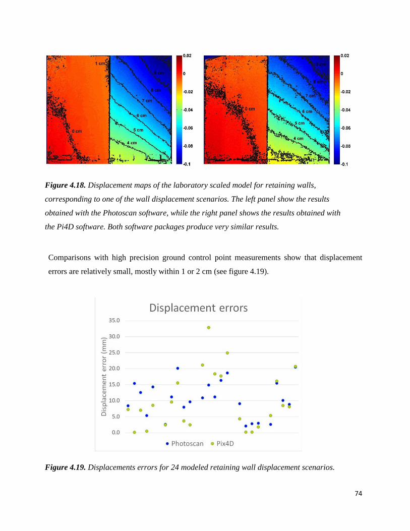
74
Figure 4.18. Displacement maps of the laboratory scaled model for retaining walls,
corresponding to one of the wall displacement scenarios. The left panel show the results
obtained with the Photoscan software, while the right panel shows the results obtained with
the Pi4D software. Both software packages produce very similar results.
Comparisons with high precision ground control point measurements show that displacement
errors are relatively small, mostly within 1 or 2 cm (see figure 4.19).
Figure 4.19. Displacements errors for 24 modeled retaining wall displacement scenarios.

75
4.4. Comparison of different methods, limitations and challenges
Direct comparison of measured displacement obtained by the different methods was attempted
when applicable, but in some cases such comparisons were not feasible. A comparison of
satellite InSAR based displacement with displacement measurements obtain from other methods
(e. g. LiDAR or digital photogrammetry) was not straightforward for any of the test sites where
we collected data. Differences in time coverage, spatial resolution and data density, and direction
of movement don’t allow for a direct, quantitative comparison between surface displacements
obtained from InSAR analysis vs. other methods. However, broad qualitative comparisons are
possible, and in the case of the Nevada site, the areas showing the larges surface displacements
derived from the InSAR analysis coincide with fieldwork inspection of the unstable rock slopes,
as detailed in Bouali et al., 2016a, and Bouali et al., 2016b.
Comparisons between digital photogrammetry and LiDAR measurements of surface
displacements are relatively straightforward. Both methods produce surface representations in
the form of point clouds that can be compared in different ways, and from which similar surface
displacement measures can be derived. In some cases the point clouds for common surface
surveyed at the same time, were very similar, with relatively small differences that could be
considered as part of the expected measurement errors. But in some cases the discrepancies
between digital photogrammetry and LiDAR results were larger than what would be expected
from random errors, and may be related with data acquisition problems, or other systematic error
inducing causes. And in some cases, such large inconsistencies were also observed between
digital photogrammetric datasets from different times, acquired over the same surface, as has
been mentioned previously.
Figure 4.20 shows the comparison of a small section of the Nevada test site rock slope that was
analyzed using digital photogrammetry and LiDAR methods. Data were acquired
simultaneously, allowing to scale the photogrammetric point cloud to best match the LiDAR
point cloud, and avoid the problem of scale mismatches previously mentioned for this site.
Although the photogrammetric data seem slightly more noisy than the LiDAR data, the surfaces
match each other within a few cm in most areas, and only differ by larger values in areas where

76
the viewing geometry of either the LiDAR of the photogrammetry acquisition procedure (or
both) was poor.
Figure 4.20. Surface representation results derived from digital photogrammetry and LiDAR.
The upper left panel shows a hillshade map produced from a LiDAR point cloud, while the
upper right panel shows the hillshade map of the same rock slope region produced from a
digital photogrammetry point cloud. The lower panel shows the differences between the LiDAR
and photogrammetry point clouds.
Each method used has advantages, but also limitations and challenges. In case of the InSAR
some of the main limitations encountered in this project include: low spatial resolution (≥ 7 m
pixels), infrequent satellite passes (≥ 10 days), displacements in only one direction (the line of
sight), data gaps in the presence of vegetation, inability to measure high deformation rates (> 4-5

77
cm/year, Crosetto et al., 2010), and a steep learning curve for the processing and interpretation of
data.
General limitations of LiDAR have been extensively documented elsewhere (e. g. Shan and
Toth, 2008), and the limitations of its application to landslides and slope instabilities have also
be documented by other authors (e. g. Derron and Jaboyedoff, 2010; and Jaboyedoff et al. 2012).
Our datasets show similar error levels to those reported in the literature for LiDAR, and from our
Nevada LiDAR datasets it is evident that displacements on the order of 10 cm can easily be
resolved. The main limitations for the use of LiDAR include: the relative short distance that can
be covered in a single scan (< 1 – 2 km), the difficulty of obtaining a complete coverage for
complex or very rugged surfaces due to the scanning perspective, accumulation of errors when
analyzing multi-scanned datasets, and a high cost of the hardware (i. e. the LiDAR instrument)
needed for surveying.
Results from the digital photogrammetry show that in some cases the method may produce
results with a quality comparable to LiDAR scanning, but some important limitations became
evident from our fieldwork: a need for precise ground control points adds to the cost and
resources that need to be invested in photogrammetric surveys. Adequate and stable lighting
conditions are needed to obtain good results. Good optical contrast and structure are needed to
produce acceptable results, although this is usually not an issue for natural surface.
4.5. Conclusions and recommendations
A wide range of surface displacement measures can be captured with the different remote
sensing methods tested in this project, applied to a variety of geotechnical assets. Strengths and
weaknesses of each method have to be considered when deciding which processing strategy is
most appropriate for each geotechnical asset monitoring case. Monitoring displacement of
extensive asset corridors or networks that may show very small displacement rates (on the order
of mm/year) may require the use of InSAR data, especially in areas with a high number of strong
reflectors, like urban areas, or rocky, desert regions. For heavily vegetated areas, with steep and
potentially quickly moving slopes, InSAR analysis may return poor results. InSAR stacking

78
methods may offer the best alternative to obtain long term deformation time series, but point
densities may be low (< 100 points per km2).
For less extensive regions, in which the focus centers on particular assets, higher resolution
methods like LiDAR and digital photogrammetry can be used to monitor displacements with
high surface point densities. Point densities of larger than 1000 points per m2 can be achieved
with such methods, and surface displacements on the order of 1 – 2 cm can be resolved. LiDAR
equipment and operation can be costly, and in many cases digital photogrammetry can be applied
to obtain comparable results, but digital photogrammetry methods usually require the
simultaneous deployment of surveying methods to establish a precise and high quality control
points network, which may add to the overall cost of such data collections. As digital
photogrammetry methods evolved it may be possible that such additional control points network
requirements could be relaxed, especially if high precision GPS location (e. g. RTK GPS)
onboard of the surveying platform (e. g. UAV) or sensor (e. g. GPS integrated camera) reduce
the camera location errors.

79
Chapter 5: Performance Monitoring and Condition Assessment
5.1 Introduction
The objective of this chapter is to evaluate and demonstrate how remotely-measured
displacement values can be used to rate the condition of geotechnical assets. Presented is a multi-
tiered approach: a large-scale, low-resolution level in which critical areas are identified for
further in-depth analysis which is performed at a local-scale, high-resolution level. Analysis of
remote sensing data gives a diagnostic performance and condition assessment of the asset at each
level, determining whether the asset needs immediate attention and further actions. If further
actions are deemed necessary, they can be assigned to either the further analysis group, where
data point to a potential hazard but additional examination is required, or the explicit actions
group, where mitigation strategies must be devised because the asset has been deemed hazardous
and may deteriorate or experience loss of performance (Schaefer et al. 2013).
The multi-tiered approach is then demonstrated on two case studies: (1) a slope stability analysis
along a railroad corridor in southeastern Nevada and (2) a retaining wall along the metropolitan
Detroit M-10 highway in Michigan. InSAR, LiDAR, and optical photogrammetry are the
specific remote sensing techniques applied to these two case studies. Similar multi-tiered
approaches can be easily adopted for any geotechnical asset along the transportation
environment.
5.2 Performance Monitoring of Geotechnical Assets
Key steps in the geotechnical asset management (GAM) program are condition assessment and
long-term performance monitoring (Sanford Bernhardt et al., 2003; Vessely, 2013). Several
authors, including Sanford Bernhardt et al. (2003), Stanley (2011), Stanley & Pierson (2013),
and Vessely (2013), have described the challenges of defining performance monitoring and
condition assessment methods. For example, Stanley & Pierson (2013) discuss the minimal data
available to aid in the understanding of geotechnical life-cycle performance under various
conditions (e.g., during maintenance, under different external stresses, etc.). Geotechnical assets

80
are expected to deteriorate. To mitigate complete failure – a disaster that could cause human
casualties and loss of infrastructure and money – periodic repair and preventative maintenance
would help reduce asset deterioration, thus extending the lifetime of the geotechnical asset.
Challenges arise when attempting to define specifics, such as the adequate level of maintenance
required, where to apply maintenance, which assets to target first, and, surprisingly, what
relevant variables to measure.
Ground movement and deformation is a key variable to measure in geotechnical asset
performance monitoring. Ground deformation has traditionally been studied using in situ
instrumentation, such as inclinometers, accelerometers, or continuous GPS monuments.
Measurements of ground displacement and/or velocity, soil moisture, and groundwater pressure
have all been correlated to slope failure (Mikkelsen, 1996). Installation and real-time monitoring
of these variables was the only method towards determining the life-cycle position of a slope (or
of the geotechnical assets built upon the slope) and, in turn, predicting the potential of a
landslide. This method is reactionary and may work for slow-moving landslides, but cannot work
for more rapid landslides where a negligible reaction time will not allow for mitigation (Zwissler
et al. 2014; Smith et al. 2015). Therefore, proactive approaches using ground movement and
deformation observations have been studied in order to hopefully predict the spatial and temporal
extent of landslide occurrences.
A hypothesis created by Fukuzono (1985) and later studied by Voight (1989) stated there is a
relationship between the strain applied to a material and the time of failure of that material.
Figures 5.1 and 5.2 demonstrate two experimental scenarios where inclinometers measured the
velocity of slope material during controlled landslides (Petley, 2004; Wartman & Malasavage,
2013). A linear inverse velocity vs time relationship has been observed in cases where brittle
deformation, or failure along pre-existing planes of weakness, occurs (Kilburn & Petley, 2003;
Petley, 2004; Wartman & Malasavage, 2013). Nonlinear inverse velocity vs time relationships
have also been observed and have been interpreted as landslides exhibiting ductile failure
mechanisms (Angeli et al., 1989; Petley et al., 2004; Petley & Petley, 2004; Federico et al., 2012;
Wartman & Malasavage, 2013).

81
Figure 5.1: Inverse velocity plots of two inclinometers undergoing (A) linear acceleration with
failure at day 180 and (B) steady-state creep until day 152 and sudden linear acceleration with
failure at day 180 (Petley, 2004).
Figure 5.2: Inverse velocity plots of two inclinometers undergoing (A) brittle failure and (B)
ductile failure (Wartman & Malasavage, 2013).
Utilizing ground deformation to monitor performance and assess condition can be applied to a
variety of geotechnical assets. Slopes along transportation corridors vary based on composition,
deformation characteristics, and failure mechanisms. Slopes may be natural, artificial, or a
combination of both. Surface deformation, observable via remote sensing techniques and not
requiring subsurface data, may reflect the movement along a deep failure surface within the soil
or rock mass of the slope. Deformation patterns can be matched with modeled deformation
(Figure 5.3) to infer the deformation mechanisms and time of future potential landslides. Slope
characteristics such as slope geometry, composition, and material strength parameters play a

82
major role in determining the stability and surface deformation patterns of a slope. Ideally, a
measure of the deformation relative to the location of neighboring points (e.g., strain) should be
considered when assessing the stability of slopes, but this task may be difficult with low
resolution datasets. The evaluation of terrain deformation needs to be done within the context of
that particular type of asset and the specific conditions under which it may fail while considering
the external factors that play into slope deformation and stability.
Figure 5.3: Surficial displacement pattern models illustrating how deep landslides may appear
in processed InSAR results (Schlögel et al., 2015).
Retaining walls also include a wide variety of designs. There are two main elements to consider
when determining retaining wall performance monitoring techniques: the retaining wall itself
and the backfill behind the retaining wall. Backfill stability may be approached similarly to slope
stability problems, but the presence of the retaining wall will obviously provide support (per its
function). Therefore, deformation monitoring may refer to data points on the retaining wall or

83
points on the backfill, depending on viewing geometry and capabilities of the remote sensing
technique. Performance monitoring and condition assessment of the retaining wall infers
information about the backfill and vice versa. The ideal situation is to acquire data on both
elements. If deformation is measured on a large enough number of points along the retaining
wall and the wall geometry is relatively simple, it is possible to model the wall as a rigid body,
allowing for more precise displacement measurements.
5.3 Remote Sensing Techniques for Geotechnical Asset Performance Monitoring and
Condition Assessment
Remote sensing techniques can be utilized for different steps incorporated into the GAM
procedure. Terrain models, including digital elevation models (DEMs), can be generated using
remote sensing. DEMs can then be used to characterize the surficial geometry adjacent to
transportation corridors; slopes can be characterized and initially classified. High resolution
imagery can also be used to rate slopes according to their stability and potential for failure or
producing rockfalls that may affect the transportation corridor.
A variety of remote sensing techniques may be used to monitor geotechnical asset performance,
including InSAR, LiDAR, and optical photogrammetry. Each of these methods have advantages
and limitations that were previously discussed. All three techniques are capable of creating
DEMs and measuring ground deformation. InSAR requires two images from different vantage
points to create a DEM, and requires at least two images to measure ground deformation, with a
larger number of images (>20) necessary to measure mm-scale ground deformations. LiDAR and
optical photogrammetry require one acquisition to create a DEM and at least two acquisitions to
measure ground deformation, with the optical photogrammetry requiring multiple images from
various vantage points per acquisition. These techniques measure surface deformation, which, as
described above, can imply deformation within the subsurface.

84
5.4 The Multi-Tiered Approach
Remote sensing techniques can be used to apply a multi-tiered approach towards performance
monitoring and condition assessment for GAM (Figure 54). For example, a large-scale level
analysis (with respect to deformation measurements) could be the identification of all slopes
along a transportation corridor that show any magnitude of deformation. Slopes that are
identified as potentially unstable through this approach can then be further examined with
targeted LiDAR and optical photogrammetry data acquisitions. The combination of all three
techniques allows for a robust identification of potential hazard regions along the transportation
corridor, as shown with the two case studies below.
Figure 5.4: Flow diagram illustrating the multi-tiered analysis process proposed for monitoring
geotechnical assets.

85
5.5 Case Study I: Unstable Slopes along Railroad Corridor in Southeastern Nevada
The Nevada study site is a railroad transportation corridor that follows the low valley topography
of a canyon system. Slopes of varying degrees of steepness (e.g., near-vertical to gently dipping)
are located along one or both sides of the route along many segments of the tracks. Most of the
slopes are composed of volcanic rock, such as rhyolite and tuff, as well as metamorphosed
welded tuff-breccia with basalt-capped plateaus upon the tallest slopes (Schaefer et al. 2015;
Bouali et al. 2016).
The railroad corridor in southeastern Nevada (Figure 5.5) is a study site that illustrates the
benefits of applying the large-scale level analysis. Utilizing a GIS shapefile of the railroad track
segment of interest, the first step of the analysis was to examine the corridor and determine what
slopes may be proximal enough to the tracks. A 1-km buffer area on each side of the tracks was
defined (Figure 5.6A). Then, using a 10-m digital elevation model (DEM) from the National
Elevation Dataset (NED), slopes located within the buffer area with a slope angle greater than
30° were identified as potentially unstable (Figure 5.6B). These slopes are potential source areas
for landslides that may affect the railroad corridor. The next step was to calculate the height-to-
length ratio (H/L) of each slope within the buffer area. An H/L threshold of 0.25 (a somewhat
conservative value) was used; H/L = 0.25 correlates to large landslides (105 to 106 m3)
according to global H/L catalogs (Hunter & Fell, 2002). Figure 5.6C shows the number of
potential landslide source locations each pixel is exposed to, with a maximum of 6,677 sources at
some locations. The final step was to incorporate ground displacement rate (velocity) data from
remote sensing techniques. For this study site, the only remote sensing technique available at the
large, regional scale was satellite-based InSAR. PSI velocity calculations for the segment of
railroad corridor is shown in Figure 5.6D. End results of this analysis can be displayed as relative
exposure map (Figure 5.6E), which spatially presents 95 and 99 percentile of relative exposure
for the railroad corridor, while Figure 5.6F displays the combined information from the exposure
map and from ground deformation derived from InSAR

86
Figure 5.5: 29-km segment (orange) of the railroad corridor study site in southeastern Nevada.
Figure 5.6: (A) 1-km buffer zone; (B) areas with slope angle > 30°; (C) potential landslide
locations due to number of source areas per pixel; (D) InSAR ground displacement rate; (E)
exposure map based on (A), (B), and (C); (F) hazard zones along railroad corridor based on (D)
and (E).

87
5.6 Case Study II: Retaining Wall on M-10 Highway in Metropolitan Detroit, Michigan
The retaining walls on the M-10 highway in metropolitan Detroit (Figure 5.7) offered a favorable
study location for detailed-scale analysis. This portion of the M-10 retaining wall was
experiencing rotational displacement (top end towards the highway) and so high resolution
optical photogrammetric imagery were collected. Point clouds generated from these imagery
were used to interpolate raster surfaces parallel to the actual wall surface with pixel values of the
distance between the optical camera and the retaining wall. Raster surfaces created from imagery
obtained at two different acquisition dates (Spring 2014 and Summer 2014) were differenced to
create a map that shows the relative displacement of the retaining wall between the acquisitions
(Figure 5.6). Light green colors represent zero displacement. Blue colors represent displacement
away from the camera and highway (into the page). Red colors represent displacement towards
the camera and highway (out of the page). Displacement magnitudes range from ±4 cm.
Displacement distributions for two segments of the retaining wall are shown in Figure 5.7, where
the green displacement distribution plot corresponds to the retaining wall between joints 3 and 4
and the blue displacement distribution plot corresponds to the retaining wall right of joint 4
(Figures 5.7 & 5.8). Figure 5.8 illustrates the displacement near two retaining wall joints and
aerial-view interpretations of wall movement. These results can then be used to infer possible
failure mechanisms and the need to mitigate a potential future wall failure at these problem
locations along the M-10 highway, if necessary.
Figure 5.7: Retaining walls and joint sets along the M-10 highway in metropolitan Detroit.

88
Figure 5.8: Displacement map along the retaining walls (Figure 5.7). Displacement is measured
in cm in a direction towards/away from the road (in and out of the page, respectively).
5.7 Conclusion
Geotechnical assets are sometimes ignored or not included in the transportation asset
management system concept. Reasons for this may include the difficulty of establishing long-
term expectations on the asset’s performance and life-cycle behavior or that monitoring the
health of a geotechnical asset may require expensive and time-consuming methodologies.
Monitoring the surface displacement or deformation of geotechnical assets, however, can be a
highly valuable approach for GAM purposes. Surface deformation can be used to infer an asset’s
internal/subsurface condition. Traditional field methods to measure ground deformation may be
an expensive and resource-intensive approach towards monitoring the state of geotechnical
assets. This project proposes the use of remote sensing methods (InSAR, LiDAR, and optical
photogrammetry) to identify and measure surface displacements across various geotechnical
assets.

89
Chapter 6: Geotechnical asset management decision support system
6.1. Introduction
A Geotechnical asset management decision support system (GAMDSS) can be defined as a web
friendly application that can be used to share information on GAM with users and facilitate its
analysis. Open source, free software is used to build the GAMDSS, which includes the client and
server software. The GAMDSS is designed to host a series of information layers that can be
managed remotely, allowing the user to upload and manage information, in the form of layers
and projects. Data types that can be managed include high resolution raster images using Web
Mapping Services (WMS), vector data types based on Google’s KML data format, vector feature
info popups, and information displayed as legends for the raster and vector data layers. The
server software runs on Linux via an Apache webserver, while the client web application is
compatible with most common web browser software, allowing in cases where there is internet
connectivity, to use the application remotely in the field.
6.2. Server Software
A software suit, including Apache, PostgreSQL, Django, and GeoServer, are used for the
GAMDSS server, all of which are open source and widely used in the web community. This
software receives web requests, processes the data, and returns a response. Apache is world’s
most used web server. PostgreSQL is an object-relational database management system. Django
is a Python based web framework. Django is used as a link between Apache and PostgreSQL,
receiving web requests from Apache and interacting with the dataset queries via PostgreSQL.
The management of the GAMDSS database content is also possible through Django, allowing
users to manage projects remotely, uploading new layers or creating new projects. Figure 6.1
shows a screen capture of the Django administration interface.

90
Figure 6.1. Screen capture of the server administration page.
An open source Web Mapping Service (WMS) called GeoServer is used in the GAMDSS to
access high resolution raster imagery. The efficiency of raster datasets display depend on the
generation, storage and display of overviews, which are reduced resolution versions of the
original raster image, and on a process called tiling, which segments images in smaller subsets
that can be transferred over the internet, instead of sending the whole original image. Tiles
produced from the tiling algorithm are compressed JPG images, which also reduces the amount
of information stored and transmitted, as compared to the original high resolution images.
Combining the overviews and tiling operation allows for greater efficiency in GeoServer
processing, as the lowest appropriate resolution overview is chosen for on-screen display. This
allows for high resolution to be used in the database, but requires its full resolution display only
for cases of very close-up viewing of the imagery.
6.3. Client Software
A combination of HTML, JavaScript and Sencha ExtJS 4.2.1., was used to build the GAMDSS
client web application. HTML and JavaScript are languages commonly used for web
applications, and ExtJS is a JavaScript application framework used by the GAMDSS to build the
Graphical User Interface (GUI) as well as the communication with the server software.

91
Several JavaScript libraries are also included in the client application, to provide geospatial
mapping functionality. Google Maps API V3 is used for generic mapping functionality which the
remaining client functionality is built from. GeoXML3, an open source KML parsing library,
enables the client application to read and display KML files. KML files, another google standard,
can incorporate both raster and vector components such as point features, line features, polygon
features, and ground overlays. Since GeoXML3 is open source, it was modified to provide
additional functionality to support the display of custom legend overlays using ExtJS, enabling
content creators greater flexibility when determining how to present information in the
GAMDSS.
6.4. User Interface
A user interface for the GAMDSS displaying a map view of the datasets allows to handle the
data and visualize different layers of information. A control panel on the right side of the
interface has the dropdown menu from which different projects or study area can be selected for
viewing. Once a project or study area has been chosen, a series of other data layers can be
selected for that specific project or site, including Hazard, Site Variable, and Ancillary datasets.
Layers can be added and displayed individually or in combinations, as both raster or vector
datasets.
Figure 6.2 Screen capture of the GAMDSS graphic user interface.

92
Legends and tags can also be displayed, depending on the zooming level of the respective layer.
Legends can be rearrange or minimized by the user, to create a more personalized and
convenient display. Depending on the nature of the datasets, zooming levels can display very
high resolution datasets, for instance, orthophotographs generated from digital photogrammetry
with a pixel size of 2 cm can be displayed at full resolution in the GAMDSS, which is a much
higher resolution than what would be allowed through Google Maps. At very high zoom levels
the map background will switch from the standard satellite imagery displayed in Google Maps,
to whatever raster layer is loaded at the time in the GAMDSS (see example in figure 6.3).
Figure 6.3 Screenshot of GAMDSS user interface at a very high zoom level.
6.5 Nevada Case Study
The GAMDSS was applied to the Alaska and Nevada field test sites, and here we present the
Nevada case study. For this example we consider the 30 kilometer railroad corridor previously
described in this report, which is subject to rockfall, slope instability, and related problems. The
GAMDSS allows three layers of data to be displayed: hazards, site variables, and ancillary.
Hazard layers include products of the performance and condition assessment analysis discussed

93
in chapter 6, which take some of the input displayed through the site variables layers, like slope,
etc. The ancillary layers provide extra information on the context of the problem, and it includes
layers like the geology, etc. Figure 6.4 shows the terrain slope (in degrees) of the Nevada test
site, as a raster layer, over a high resolution satellite imagery background, i. e. the standard
Google Maps high resolution satellite imagery background.
Figure 6.4 Slope map of the Nevada test site.
Figure 6.5 shows the geology layer contained in the ancillary layer dataset. Information on the
geological units from this layer can be displayed by clicking on the map units. Other information
that can be displayed for the geology layer includes the area, perimeter, USGS standard
nomenclature, etc. Similar capabilities would apply to other ancillary data layers (e. g. faults,
etc.).

94
Figure 6.5 Screen capture of the geology and regional faults layers displayed in the GAMDSS.
The hazard category contains layers that are related to slope performance and long term stability.
Figure 6.6 shows the surface velocity derived from InSAR data, for the Nevada test site. InSAR
analysis was based on European Space Agency (ENVISAT satellite) radar images, as described
in chapter 5. The displayed points correspond to individual pixels, with colors corresponding to
the magnitude of the displacement velocity (red is downward and flue is upward) within ± 20
mm/year. Many different information fields can be associated to each layer and with each
element in a layer, in this case, with each point where velocity has been measured, including the
average velocity value, the total displacement, individual displacement between successive
InSAR images, etc.

95
Figure 6.6. Ground velocity (mm/year) data displayed across the Nevada study area.
6.6. Conclusion
Decision support systems applied to geotechnical asset management can be a useful tool for
visualizing and analyzing data in a geographic information system environment. The GAMDSS
provides a solution that incorporates hazards, site characteristics and ancillary information
provided by the user, in a single web based platform. The GAMDSS uses open software tools, it
is designed to be user friendly, and easily accessible from most web platforms.
High resolution raster dataset can be displayed in the GAMDSS through GeoServer, while vector
data in .kml format can also be added as data layers. The study case for the Nevada test site
presented in this chapter show how the GAMDSS can be used to display information that is
useful for asset management purposes.

96
Chapter 7 Cost-benefit analysis of remote sensing methods applied to geotechnical asset
management
7.1. Estimating costs of different technologies and platforms
Two scenarios are considered for estimating costs, an “in-house” built capacity and an
outsourcing scenarios. In the “in-house” scenario the physical resources and knowledge
necessary to apply the method are acquired or developed within the transportation agency or
transportation system administrator. Costs associated with the “in-house” scenario include the
initial investment in equipment, analysts and operators training, and long term cost of operation.
In the outsourcing scenario the different services are hired or contracted to a company or
commercial provider, to obtain a final product, e. g. point clouds or other surface representations
from a LiDAR or digital photogrammetry survey. To compare both types of scenarios, costs will
be annualized when possible, and initial investment cost will be distributed over a period of time
estimated to be equivalent to the useful time for the equipment or technology.
The estimation of whether the “in-house” or the outsourcing scenarios are a better choice for an
agency depends on many factors, including the scale of the agency’s budget, the volume of work
that would be routinely done using the technology under consideration, and other factors. Large
budget and extensive work volumes may require developing “in-house” capabilities, which may
be more costly initially (e. g. due to initial investment), but could pay off on the long run, as the
initial investment is recovered, and subsequent availability of in-house capabilities results in cost
savings. Smaller budgets and relatively low work volume cases may be more efficiently dealt
with through outsourcing. The choice between the “in-house” vs. the outsourcing options may
also depend on whether a technology in questions is available in both or only one forms.
7.2 Satellite based InSAR costs
Costs for development of “in-house” InSAR analysis capabilities include initial investment costs
of buying software and hardware, and developing the knowhow, i. e. technical training of
personnel. Sustained operation costs include computer time and related costs (data storage, etc.),

97
as well as the operators and analyst salaries. Data acquisition costs depend on the type of radar
images used, but can also be substantial if stacking methods requiring tens of images to be used.
For the purpose of cost comparisons, a standard work volume scenario is considered, and the
costs of the data analysis for both “in-house” and outsourcing will be referred to such scenario.
The scenario considers between 1 and 10 locations being analyzed, over a corridor length
between 100 and 1000 miles. Table 8.1 shows the costs of different types of radar satellite
images, and the time periods they cover, as well as revisit period and ground resolution.
Table 7.1. InSAR satellite images characteristics.
Satellite Mission Timespan
Revisit Period (days)
Ground Resolution
(meters)
Price Per Image (US Dollars)**
ERS-1 1991 - 2000 35 25 $212 - $354 ERS-2 1995 - 2011 35 25 $212 - $354 RADARSAT-1 1995 - 2013 24 10-100 $3,047 - $3809 ENVISAT 2002 - 2013 35 25-150 $354 - $591 ALOS PALSAR
2006 - 2011 46 7-100 $42 - $709
RADARSAT-2 2007 - 24 3-100 $3,047 - $7,110 COSMO-SkyMed
2007 - 16 1-100 $680 - $2,268
TerraSAR-X 2007 - 11 1-16 $875 - $7,972 Meteor-3M 2009 - 3 400-1,000 $30/$40 - ? ALOS PALSAR-2
2014 - 14 1-100 $1,257 - $4,191
Sentinel-1A 2014 - 12 4-80 Free of cost SEOSAR/Paz 2015 - 11 1-15 Will be publically available Sentinal-1B 2016 - 6 4-80 Will be publically available COSMO-SkyMed 2nd Generation
2016 - 1.5-10 1-35 Will be publically available
**US Dollar exchange rates (January 2015). NA = not available for commercial or educational use. Prices and data availability listed for users in the United States.
Table 7.2 summarizes the expected “in-house” costs for an initial investment in hardware and
software, and the long term operational cost associated with labor and data storage, as well as
radar images cost. Table 8.3 summarizes our estimation of outsourcing costs for the InSAR
analysis.

98
Table 7.2. Summary of costs for in-house InSAR analysis capacities
Item Cost estimate Low High
Computer hardware 1,500 2,500 Software 8,000 65,000 Annual data storage 4,000 4,000 Annual analyst labor 3,200 16,000 InSAR images 20,000 200,000 Total 36,700 287,500
Table 7.3. Summary of costs for outsourcing the InSAR analysis
Item Cost estimate Low High
Outsourcing InSAR analysis 20,000 250,000 Total 20,000 250,000
7.3 LiDAR costs
LiDAR costs are strongly related to the platform from which the data are acquired. Aerial
LiDAR costs can be very high because of the aerial platform, and the high power laser involved
in the scanning. Costs presented by Vincent and Ecker (2010) for aerial LiDAR ran as high as $
8321 per mile of corridor (see also discussion of this case in Chang et al. 2014). Table 8.4
summarizes the costs for the “in-house” LiDAR case using a standard work volume scenario.
Table 7.4. Summary of costs for in-house capacities for aerial LiDAR analysis
Item Cost estimate Low High
Total (non-itemized) cost 25,200 541,000 Total 25,200 541,000
For practical purposes most agencies are likely to outsource aerial LiDAR work. The outsourcing
costs depend on the work load and the type of products that are required, a study by the USGS
National Data Elevation Assessment reported costs ranging from $ 90 to $ 521 per square mile,
for large areas surveyed (> 5000 sq. mi) in 2012, while the State of Michigan reported costs

99
between $ 100 and $ 250 per square mile, for similarly large surveys in 2013 (State Of Michigan
Center For Shared Solutions, 2013). Slightly higher costs of $ 335 were reported for Wisconsin
in 2014 (McDougal, 2014), and $ 344 per mile estimated for Vermont in 2015 (Vermont Center
for Geographic Information, 2015). This gives us an idea of the likely range of prices that could
be encountered in the market. Applied to our standard work scenario, the estimated costs are
presented in table 8.5.
Table 7.5. Summary of costs for outsourcing the aerial LiDAR analysis service
Item Cost estimate Low High
Outsourcing LiDAR analysis 25,000 521,00 Annual data storage 200 20,000 Total 25,200 541,000
Mobile LiDAR costs have been documented by Vincent and Ecker (2010), Yen et al. (2011 and
2014), and Chang et al. (2014), including initial investment and long term operation costs. As
with previous cases the costs depend on the types of data being collected and the expected final
products being delivered to the client. Table 6 summarizes our “in-house” estimate of mobile
LiDAR costs.
Table 7.6. Summary of costs for in-house mobile LiDAR expertise
Item Cost estimate Low High
LiDAR instrument 5,000 200,000 Analysis software 500 80,000 Computer hardware 1,500 2,500 Annual data storage 60 600 Ground control surveying (rapid)1 38,500 531,000 Ground control surveying (high accuracy)1 993,300 9,933,000 Data processing labor 24,000 240,000 Total (with rapid control)1 69,560 1,054,100 Total (with high accuracy control)1 1,024,360 10,456,100 1Two sub-scenarios are considered here, depending on whether rapid or high accuracy ground control is used.

100
Cost of outsourcing mobile LiDAR have been documented recently by Yen et al. (2014).Applied
to our standard work scenario, the expected costs are shown in table 8.7.
Table 7.7. Summary of costs for outsourcing the mobile LiDAR analysis service
Item Cost estimate Low High
Outsourcing mobile LiDAR service (rapid control) 42,200 717,000 Outsourcing mobile LiDAR service (high accuracy control) 1,000,200 10,000,000
Costs of terrestrial LiDAR are also influenced by the type of equipment used, and the expected
products characteristics (e. g. point density, precision, etc.). Terrestrial LiDAR is usually
required for the highest point densities and highest precisions. Vincent and Ecker (2010)
estimated costs as high as $ 29,258 per mile for this kind of survey. Applying their data to our
standard working scenario we estimate the costs summarized in table 8.8 for the “in-house” case.
Table 7.8. Summary of costs for in-house terrestrial LiDAR expertise
Item Cost estimate Low High
LiDAR data collection and analysis (high accuracy control)1 100,000 1,000,00
0 LiDAR data collection and analysis (rapid control)1 72,000 760,000 Annual data storage 200 2,000
Total (with high accuracy control)1 100,200 1,002,00
0 Total (with rapid control)1 72,200 760,000 1Two sub-scenarios are considered here, depending on whether rapid or high accuracy ground control is used.
Outsourcing costs for terrestrial LiDAR have been reported by Chang et al. (2014), as
summarized in table 8.9, and fall in a similar range compared with the “in-house” cost ranges.
Table 7.9. Summary of costs for outsourcing the terrestrial LiDAR service
Item Cost estimate Low High
Outsourcing terrestrial LiDAR service 100,200 1,002,000 Total 100,200 1,002,000

101
7.4 Digital photogrammetry costs
Costs for “in-house” UAV base digital photogrammetry were estimated from our experience of
developing the system used in the project. Long term operation costs are somewhat uncertain,
give that this is a relatively new and still emerging technology. Table 8.10 summarizes our
estimates for the costs of UAV based photogrammetry applied to our standard work scenario.
Table 7.10. Summary of costs for in-house UAV SFM photogrammetry expertise
Item Cost estimate Low High
UAV 500 10,000 Camera 1,000 4,000 Computer hardware 1,500 2,500 Analysis software 2,000 15,000 Surveying equipment 5,000 50,000 Annual data storage 500 5,000 Data collection labor 20,160 32,000 Data processing labor 6,720 10,667 Ground control surveying (rapid ground control)1 4,000 80,000 Ground control surveying (high accuracy control) 1 10,000 200,000 Total (with rapid ground control) 1 41,380 209,167 Total (with high accuracy ground control) 1 47,380 329,167 1Two sub-scenarios are considered here, depending on whether rapid or high accuracy ground control is used.
Estimating an outsourcing cost for the UAV based digital photogrammetry is not
straightforward, as such services are just now beginning to be offered, but the costs could be
similar to the “in-house” option detailed in table 8.10.
Terrestrial digital photogrammetry costs are expected to be similar to the UAV based
photogrammetry, but without the cost of the UAV. Longer fieldwork required for data
acquisition may however increase the costs of terrestrial digital photogrammetry, as terrestrial
based photogrammetry may have less advantageous perspectives from which to acquire data.
Table 8.11 summarizes our cost estimates for the “in-house” terrestrial digital photogrammetry
scenario.

102
Table 7.11. Summary of costs for in-house terrestrial SFM photogrammetry expertise
Item Cost estimate Low High
Camera 1,000 4,000 Computer hardware 1,500 2,500 Analysis software 2,000 15,000 Surveying equipment 5,000 50,000 Annual data storage 500 5,000 Data collection labor 20,160 32,000 Data processing labor 6,720 10,667 Ground control surveying (rapid control)1 4,000 80,000 Ground control surveying (high accuracy control)1 10,000 200,000 Total (with rapid control)1 40,880 199,167 Total (with high accuracy control)1 46,880 319,167 1Two sub-scenarios are considered here, depending on whether rapid or high accuracy ground control is used.
As with the UAV digital photogrammetry outsourcing case, the costs estimates are mostly
hypothetical considerations, given that such services are not yet widely available, and their costs
haven’t been observed in a real market. Similar costs to “in-house” implementation is also
expected, as described previously in table 8.11.
Mobile digital photogrammetry is an even less explored technology than aerial or terrestrial
based digital photogrammetry. Costs of “in-house” mobile photogrammetry include some of the
costs discussed for photogrammetry in previous sections, but due to the different platform the
type of sensor is also different. Hardware and software costs for this kind of photogrammetry are
summarized in table 8.12

103
Table 7.12. Summary of costs for in-house mobile SFM photogrammetry expertise
Item Cost estimate Low High
RED Epic-X Camera 40,000 50,000 Computer hardware 1,500 2,500 Analysis software 2,000 15,000 Surveying equipment 5,000 50,000 Annual data storage 500 5,000 Data collection labor 20,160 32,000 Data processing labor 6,720 10,667 Ground control surveying (rapid control)1 4,000 80,000 Ground control surveying (high accuracy control)1 10,000 200,000 Total (with rapid control)1 79,880 245,167 Total (high accuracy control)1 85,880 365,167 1Two sub-scenarios are considered here, depending on whether rapid or high accuracy ground control is used.
Due to the early stages in development of the mobile photogrammetry it is difficult to estimate
the cost of outsourcing this kind of service, but as with previous cases, costs may be similar to
those of “in-house” development of the capabilities.
7.5. Benefits from each technology and comparison with their costs
The ultimate goal of a cost-benefit analysis is to compare both elements (costs and benefit) in
terms of their monetary value, although this can be a very complex, and sometimes controversial
process (e. g. Boardman et al., 2006; Zerbe and Bellas, 2006). For the remote sensing methods
that produce results in a point cloud format described in this report (i. e. LiDAR and digital
photogrammetry) we will consider benefits in terms of two main criteria of value, reflecting the
information content of the products derived from these methods, and which are mostly relevant
to the geotechnical hazard assessment process: sampling point precision and point surface
density. Sampling point precision describes how close a sampled surface point is to the real
location of the surface in three dimensional space. Point surface density describes how many
sampling points are retrieved per unit of surface area of the geotechnical asset that is being
surveyed. In the case of InSAR, the quality of the results cannot be evaluated in terms of the

104
precision of point locations, but rather in terms of the precision of the measured surface
displacement. The surface point density criterion is also applicable to InSAR.
Typically sampling point precision for close range (< 25 m from sensor to target) terrestrial
LiDAR and photogrammetry tends to be within the 1 to 2 cm range, as has been documented in
chapters 4 and 5. This values can easily degrade to > 10 cm in the case of digital
photogrammetry, if the ground control is poor, or the acquisition conditions are unfavorable. For
purposes of comparison we will take the optimistic scenario of data acquisition in good
conditions and use the 1 to 2 cm for the sampling point precision. Mobile and aerial LiDAR
sampling point precision is usually is not as good, typically in the range of 5 to 30 cm (Shan and
Toth, 2009). InSAR surface displacement precision along the line-of-sight direction is usually on
the order of a few millimeters (Crosetto et al., 2010; Ferretti et al., 2011).
Point densities for LiDAR datasets depend on the setting of the scanner and the distance to the
surface being scanned. Some LiDAR scanners can survey a surface at 0.01º increments, resulting
in a 1.7 cm distance between points at 100 m distance. Point densities for digital
photogrammetry datasets depend on the cameras sensor resolution, the focal length of the optical
system, and the distance to the surface being imaged, as well as how many of the pixels in the
images are chosen for re-projection onto the three-dimensional surface produced by the model.
Figure 7.1 shows the distance between points as a function of distance for LiDAR and optical
photogrammetry, assuming reconstruction of the surface using all the pixels.
Figure 7.1. Separation between surface sample points for cases discussed in the text. LiDAR line corresponds to a 0.01º scanning increment. The other lines correspond to photogrammetry with different focal lengths, as indicated.

105
InSAR point densities vary from relatively high in areas where continuous interferograms can be
generated from pairs of radar images, to very sparse in areas where only staking techniques can
retrieve some isolated points. In the case of continuous interferograms the point density will be
limited by the radar image resolution, which typically falls in the 1 to 100 m size category. In the
case of stacking methods like the PSI algorithm the densities can be much lower, and for the sites
where we had successful displacement measurements (e. g. the Nevada test site), the point
density was on the order of 7 x 10⁻⁴ points per m2, which would correspond to an average
distance between points of ~ 38 m.
7.6 Synthesis of costs and benefits.
Costs and benefits described in this chapter can be summarized in table 8.13, although a
monetary value for the benefits is not given, and only a proxy of their value, defined by the two
information content criteria (precision range and point density), are given.

106
Table 7.13. Costs and benefits, described as information content, from each technology
Type of survey Cost estimate ($) Precision
range (mm)
Point densities
range (per m2)
Low High Low High Low High InSAR (In-House, persistent scatterer) 36,700 287,500 2 10 10-5 10-2
InSAR (In-House, interferogram) 36,700 287,500 2 10 10-2 1 InSAR (Outsourced, persistent scatterer) 20,000 250,000 2 10 10-5 10-2
InSAR (In-House, interferogram) 36,700 287,500 2 10 10-2 1 Aerial LiDAR 25,200 541,000 50 250 102 104 Mobile LiDAR (In-House, rapid control) 69,560 1,054,10
0 50 300 102 104
Mobile LiDAR (Outsourced, rapid control) 42,200 717,000 50 300 102 104
Terrestrial LiDAR (rapid control) 72,200 760,000 10 50 102 104 Terrestrial LiDAR (High accuracy control)
100,200
1,002,000 3 20 102 104
UAV photogrammetry (rapid control) 41,380 209,167 80 100 102 104
UAV photogrammetry (High accuracy control) 47,380 329,167 30 50 102 104
Terrestrial photogrammetry (In-House, rapid control) 40,880 199,167 70 100 102 104
Terrestrial photogrammetry (In-House, high accuracy control) 46,880 319,167 20 50 102 104
Mobile photogrammetry (In-House, rapid control) 79,880 245,167 70 100 102 104
Mobile photogrammetry (In-House, high accuracy control) 85,880 365,167 20 50 102 104
7.7. Conclusions
Costs of the different remotes sensing technologies applied to geotechnical asset management
vary over a wide range, depending on the type of technology and the requirements of the
products expected from it. The relationship between the cost and the usefulness of the
information (i. e. the benefit) obtained from those methods tends to be inverse, methods that
provide more detailed and precise information tend to be more expensive. Using standard
scenarios for the required work to be done it is possible to compare the different technologies at

107
a qualitative level. The final choice between using different methods will not only be dictated by
the cost, but also by the value of the resulting information, and whether a certain type and quality
of information is needed in a particular geotechnical asset management application.
In-house capabilities development vs. outsourcing of services will depend on the agencies or
users budget, and the possibility of recovering the initial investment and long term operation
costs, of an in-house operational system.
Methods that produce very high point densities, like LiDAR and digital photogrammetry may be
necessary for applications where surface displacements change rapidly over small distances, but
such methods are not very practical to apply over very large distances. Satellite based InSAR on
the other hand can be applied to much larger areas, and can retrieve very small displacements,
although the data point density is relatively sparse, and would not work to monitor surface
displacements that change rapidly over small distances.
Consideration of all these factors, together with the costs, and in context with the agencies
budget and the problem’s needs for information will ultimate inform the decision of what
methods are more appropriate to use in each geotechnical asset management case.

108
Chapter 8: Remote sensing implementation framework
The development of new approaches to administration and operation of transportation systems
require the adaptation of traditional procedures and practices to the goals and methods inherent
in such new approaches. Such is the case for adapting transportation agency practices to the new
paradigm of transportation asset management, and a large effort has been made by federal and
state agencies in facilitating such transition (e. g. FHWA, 1999; Cambridge Systematics, Inc., et
al., 2002; USDOT 2015). In the case of geotechnical asset management, the adoption of such
practices has been slow (Vessely, 2013), in part due to the difficulty to monitor geotechnical
assets and predict the life-cycle performance.
Throughout this report we have explored, selected, and evaluated a series of remote sensing
methods that show potential to be used as monitoring techniques in geotechnical asset
management. Chapters 1 through 5 give an overview of the transportation asset management
process and details about its implementation, as wells as the details on the remotes sensing
techniques considered for geotechnical asset monitoring. In this chapter we expand on how such
methods can be incorporated in a geotechnical asset management system, considering practical
constraints.
8.1 Using geotechnical asset monitoring information and adopting remote sensing methods
for geotechnical asset management.
8.1.1 Steps to implement a geotechnical asset management system.
8.1.1.1 Prior work on asset management implementation.
Implementation of a transportation asset management system can be a challenging process.
Several authors have made an effort to document and explain how the implementation process
can be developed. The AASHTO report (AASHTO 2013) on transportation asset management
implementation is a major milestone among such efforts. Following the initial efforts to defined
and describe the concepts and practical issues behind transportation asset management (e. g.

109
Cambridge Systematics, 1999; AASHTO 2002) it was recognized that the implementation
process required a detailed, step-by-step description, resulting in the AASHTO 2013 report,
which complements earlier key reports on transportation asset management. The AASHTO 2013
report was divided in two parts, each part targeting one of two main user audiences: executive
managers and practitioners. The report also includes case studies on transportation asset
management implementation in a series of appendices. The report covers transportation asset
management in general, but geotechnical assets require a more specific treatment, and the
implementation for such a system has to be based on such specific considerations. Vessely
(2013) considered the specific case of geotechnical asset management implementation,
presenting many examples of asset management program that include geotechnical asset in their
operation. The components of a geotechnical asset management program are also presented and
compared with the actual practices at the time the report was written. A template on how to
develop a geotechnical asset management program is also presented by Vessely (2013), with
further recommendations on how to implement such a system in practice. It is also important to
remember that geotechnical asset management should ideally not be done in isolation, it should
be done as part of a large an more general transportation asset management system, and in that
sense, both the general transportation asset management and the more particular geotechnical
asset management approaches need to be considered in detail. The literature on asset
management implementation in general, and geotechnical asset management implementation in
particular has expanded since these seminal reports were published, and include some more
focused and particular study case examples (e. g. Cambridge Systematics, 2009). We borrow and
build upon these ideas to outline a general implementation process for geotechnical asset
management that incorporates the remote sensing techniques described in this report, for asset
monitoring purposes. We advise the reader to consult these reports for a more detailed treatment
of the subjects outlined in this chapter.
8.1.1.2 Defining geotechnical asset management system goals and aligning them with the
agencies general goals and objectives.
A first step in establishing a transportation asset management system is to define goals and
objectives for the system, which should align with the agency’s goals and objectives, AASHTO

110
(2013) gives a detailed overview of this step. This obviously requires that the agency has clearly
stated goals and objectives, which in some cases may not be explicitly defined. Assuming that
such general agency goals and objectives are defined one would have to consider how the
geotechnical assets contribute to such goals and objectives, and how their management can more
effectively lead the agency in achieving the goals and objectives. Starting by considering the
service that a transportation system provides to the public or to specific users, one can establish
performance metrics to evaluate how well the system is behaving. In transportation asset
management systems it is common to state performance levels in terms of the “levels of service”
standard. Characteristics such as traffic volumes, time delays and traffic congestion, road surface
smoothness, and vehicle (and ultimate driver and passenger) safety are usually important
variables that are subject to meet standard goals. Reaching those goals at the least possible cost is
a general objective of the transportation asset management system. Many other criteria can be
defined to assess the performance of geotechnical assets, for instance Table 8.1 shows a
comparison of performance measures under the MAP-21 Act and the AASHTO defined
performance measures. Although many of the performance measures in that table may not
directly relate to geotechnical assets, establishing how the performance of a particular asset
impacts those overall performance measures is a way to assess the asset’s importance.
Table 8.1 Performance measures established by the MAP-21 Act and the AASHTO TAM
Implementation Guide. Taken from AASHTO 2013.
MAP-21 Act AASHTO Implementation Guide
Safety Safety
Infrastructure Condition
Congestion Reduction Mobility
System Reliability Reliability
Freight Movement and Economic Vitality Mobility and Reliability
Environmental Sustainability Externalities
Reduced Project Delivery Delays Mobility and Reliability
Life-Cycle Cost
Customer Measures

111
Geotechnical assets usually support other types of assets (e. g. pavement, bridges, etc.).
Degradation in the performance of geotechnical assets can result in damage to other assets and
their corresponding degradation in performance, e. g. excessive terrain deformation associated to
geotechnical asset degradation (e. g. a retaining wall displacement) can reduce the road surface
smoothness. In the most extreme cases the performance degradation of geotechnical assets can
directly compromise road and traffic safety. Intermediate cases are also possible, if the damage
to the road surface is too severe or the safety is compromised, the agency may have to partially
or completely shut down some road lanes, or even the entire road, until the situation is corrected.
Considering the agency’s goals in operating the transportation system, the first step in setting
goals for the performance of geotechnical assets is to evaluate how their performance would
impact the overall performance of the transportation system, as evaluated against the agency’s
goals. For instance, how would excessive deformation along any segment of a system of
retaining walls impact traffic volumes, or delay times, or even the safety of drivers and
passengers. At this step it may be useful to look at past records of geotechnical asset related
problems and estimate the impact and disruption these problems caused for a transportation
network or corridor. If the frequency and magnitude of such disruption can be estimated from
past events, it may be a rough approach to estimate the importance for different disruption
scenarios. A more advanced treatment would include some sort of “life-cycle performance”
analysis, as it is sometimes done for other types of assets, e. g. pavements, but such approaches
are not possible in most cases, where information on the long term behavior and expected
performance of geotechnical assets is not available. The actual assessment of such scenarios
would be part of a different step in the process and will be discussed in more detail later.
8.1.1.3 Defining and prioritizing geotechnical assets, and creating and maintain an asset
inventory.
A first step in assessing the performance of geotechnical assets is to establish what types of
assets will be considered in the management system, and how they will be characterized. The
variety of asset types that could be considered can be very broad. For example, depending on the

112
terrain and other external variables, features such as slopes, both artificial and natural, can be
considered geotechnical assets. Defining whether natural slopes fall within the geotechnical asset
category can make a very large difference in the size of the asset inventory. Therefore, clearly
defining the criteria of what elements are included in the geotechnical asset inventory is critical
to the implementation of the management system. On the other hand, leaving out critical assets
can also be very problematic, as their degradation and failure could have a very large and
detrimental impact on the agency’s goals. Guidelines provided by some authors, like Sanford-
Bernard et al. (2003) and Vessely (2013) can be a starting point, but in-house expertise at the
different agencies will probably be the main resource in establishing such a classification, and
deciding what items should be considered part of the geotechnical asset inventory.
Vessely (2013) for instance identified 10 types of geotechnical assets (see table 8.2). Each of
these assets can be subdivided into more classes. Some types may be more critical, or their
failure may have a much larger impact than others, such geotechnical assets will have priority
over other assets when including them into an asset management system. Some asset types, may
be very extensive, poorly delimited or difficult to define as part of an inventory, e. g. natural
slopes next to a transportation corridor.

113
Table 8.2 Types of geotechnical assets that could be included in an asset management system.
Taken from Vessely (2013).
Geotechnical asset type Reference
Embankments and Slopes (to include rock slopes, cut slopes, landslides, and rockfall sites)
Bernhardt and others (2003) Perry and others, cuttings (2003) Perry and others, embankments (2003) Kelly (2005) Stanley and Pierson (2011) American Association of Highway and Transportation Officials (AASHTO) (2011a)
Tunnels Bernhardt and others (2003) AASHTO (2011a)
Earth Retaining Structures (retaining walls, reinforced soil slopes, and earth and rock buttresses)
Bernhardt and others (2003) Brutus and Tauber (2009) DeMarco and others (2010) Stanley and Pierson (2011)
Culverts or Drainage Channels Bernhardt and others (2003) DeMarco and others (2010) AASHTO (2011a)
Foundations Bernhardt and others (2003) Stanley and Pierson (2011)
Pavement Subgrade Bernhardt and others (2003)
Subgrade and Land within Right-of-Way United Kingdom Department for Transport (2003)
Buried Reinforcing Elements, Rock Bolts, Tieback Anchors, and other Buried Structural Elements
Stanley and Pierson (2011)
Material and Quarry Sites Stanley and Pierson (2011)
Horizontal Drains Stanley and Pierson (2011)
A stepwise process in which different types of assets are progressively included, as the agency
gains experience in the management of certain geotechnical assets, may be a way to approach the
development of a geotechnical asset inventory. Developing an inventory implies a detailed
survey of the entire transportation corridor network. Examples for retaining walls are given by

114
several authors, e. g. De Marco et al. (2010) and Anderson et al. (2008). To develop the
inventory a database has to be setup in an efficient way, with all relevant fields to record the
asset characteristics, and to allow maintaining and expanding the database in the future. Not only
is the database important for the initial inventory, but it is the base for the long term performance
assessment that will be discussed in the next sections.
8.1.1.4 Assess and monitor the performance and health for the assets in the inventory
Monitoring the asset’s performance and health on the long term is critical to the geotechnical
asset management system. It is through such monitoring that any actions to maintain, repair, and
avoid major performance degradation and related impacts, can be avoided. In the case of
geotechnical assets the performance assessment can focus different characteristics of the
geotechnical asset, but here we will focus on the surface displacement characteristics that could
indicate that the asset performance is degrading, or worse (e. g. imminent failure or collapse).
A multi-tier system as the one described in chapter 5 for performance monitoring can be
implemented to assess the state of geotechnical assets based on their surface deformation
patterns. As has been explained in that chapter (and the corresponding deliverable), the surface
deformation may be related in some cases to possible asset performance degradation, but in some
cases this may be difficult to infer, making the process less straightforward, and requiring more
in depth analysis, possibly involving in situ testing and geotechnical modeling. However the
hierarchical system should allow for an optimal use of resources, assigning priorities only to
critical cases that could have a large impact. Performance degradation of geotechnical asset may
not always be reflected by surface deformation patterns (e. g. underground erosion through
hydraulic piping may not reflect as surface deformation until the damage to the asset is
significant), for this reason, some asset may require other additional monitoring methods, but
such cases are beyond the scope of discussion in this report.

115
8.1.2 Local and regional implementation using GIS visualization and decision support
systems
Local and regional implementation of a geotechnical asset management system will require the
visualization of the information in a geographic framework. The decision support system
presented in chapter 6 provides a convenient platform to display and analyze asset performance
data over a large geographic area (e. g. the first level of a hierarchical, multi-tier asset
management system). The multi-tier approach has been also detailed in chapter 5, where
different datasets are presented for a railroad corridor, and depending on the resolution of the
dataset, different scales of analysis are required.
8.2 Transportation agencies limitations to adopt remote sensing methods for geotechnical
asset management, and ways to overcome them
Common limitations and challenges that transportation agencies may face to adopt remote
sensing methods for geotechnical asset management will include the lack of expertise on remote
sensing methods and geotechnical asset management, the investment on hardware and software,
and the long term nature of the benefits. Constrained by tight budgets and the need to invest
resource in extensive transportation infrastructure networks, transportation agencies many time
struggle to invest in activities that only will prove beneficial on the long term, and one important
part in the geotechnical asset management implementation process is to build a strong case for
such a long term investment.
Uncertainties in the long term outcomes of preventive maintenance, especially in cases where
damaging events are less frequent (e. g. landslides), can make it hard to make a convincing
argument for implementation of a geotechnical asset management system. Fortunately, extensive
documentation and economic analysis in support of the long term benefits for transportation
asset management can help to make a convincing argument. For other types of assets (e. g.
pavements, bridges, etc.) the existing life-cycle management data help to make a solid argument,
the lack of such data an models for geotechnical assets present a challenge, but the use of crude
estimates of loss, disruption and other costs associated to degrading performance (or even failure

116
and collapse) of geotechnical assets, may provide strong enough evidence for the need of
managing such assets on the long term. Collecting and analyzing such data may be in itself a
difficult task, but it could be a catalytic that sparks the interest in a larger asset management
program.
Costs of equipment (hardware and software), as well as technical personnel training, operators
and analysts salaries, and other long term sustained costs, as shown in chapter 7, may bring the
total cost of geotechnical asset monitoring over the budgetary limits of some transportation
agencies. Depending on the extensiveness of the assets to be monitored, the likelihood that
monitoring will provide valuable information for intervention of critical assets, and the
accessibility to the resources needed for monitoring the assets, different options may be
available. “In-house” vs. outsourcing of services to acquire and analyze data on asset monitoring
will depend on individual project costs, and cumulative costs over longer periods of time. If the
use of a remote sensing method for monitoring a geotechnical assets is only occasional and the
volume of work is relatively small, it may be more effective to outsource such a task. If on the
other hand the required monitoring is extensive and has to be done very frequently, or even
continuously over a large area, it may be more cost effective to develop the remote sensing
capabilities as “in-house” procedures.
Developing “know-how”, and human (technical and analytical) resources also implies a
commitment from part of the workforce at the transportation agency. The training on many of the
remotes sensing methods will not only be useful for the purposes of geotechnical asset
management, but could also be used for other task within the transportation agency. Such an
investment could therefore be viewed beyond the sole purpose of the geotechnical asset
management system. The discussion on the other strategies to overcome the limitation and
challenges of implementing a geotechnical asset management system could be expanded to the
broader agency goals and objectives, but this will of course depend on the specific goals and
objectives in each agency’s case.

117
8.3 Example of remote sensing implementation on case study sites, and possible expansions
to a complete network
8.3.1 Unstable slopes asset management example: Hypothetical case for the Portuguese
Bend Landslide Complex (PBLC) on the Palos Verdes Peninsula in California
The Portuguese Bend Landslide Complex (PBLC), shown in Figure 8.1, is a collection of
complex landslides across the rolling hills of the Palos Verdes Peninsula, southwest of Los
Angeles, California. The study area, which not only includes active landslides but ground
subsidence and uplift to lesser magnitudes, includes both urban and rural areas. Urban areas most
notably include Rancho Palos Verdes and San Pedro, which incorporates part of the Port of Los
Angeles within its city limits. Rural areas, relatively speaking, include Rolling Hills, located
nearby the active landslide area (Figure 8.2).
Figure 8.1: Palos Verdes Peninsula in California.

118
Figure 8.2: Active landslide area of the PBLC (image taken from Merriam 1960).
In order to illustrate the implementation of a remote sensing-based geotechnical asset
management approach, the following sections will include steps undertaken by the project team.
Steps include defining system goals and objectives, developing a methodology to prioritize
geotechnical assets, and assessing and monitoring long-term performance of the geotechnical
assets. This case study was implemented by processing satellite radar imagery using the
Persistent Scatterer Interferometry (PSI) technique, which is an InSAR stacking method used for
monitoring small-scale (mm) deformations over long periods of time.
8.3.1.1 Defining geotechnical asset management system goals for the PBLC case, and
aligning them with the general goals and objectives of the transportation agency.
The goals of geotechnical asset management is to proactively achieve and maintain geotechnical
asset life-cycle performance, which include user safety, transportation corridor preservation, and
minimize economic and environmental impacts of potential hazards. Geotechnical assets of
interest within the Palos Verdes Peninsula include slopes (PBLC) and urban assets (e.g., bridges,
retaining walls, etc.).

119
In order to determine the general goals and objectives of the remote sensing-based geotechnical
asset management system, the project team (a term that can be replaced by transportation agency
if implemented in the real world) conducted a literature review of previous InSAR-related
research in the region. The most recent study was conducted by Calabro et al. (2010); they
utilized ERS-2 radar images to monitor seasonal fluctuations in landslide magnitudes between
1995 and 2000. Since this study focused on data acquired 16 years ago, the project team searched
for synthetic aperture radar (SAR) single look complex (SLC) images more recently acquired.
Two proposals were submitted to acquire high resolution satellite-based SAR SLC images. The
first proposal, entitled “Using satellite remote sensing for landslide life-cycle monitoring and
failure prediction,” was submitted to and accepted by the European Space Agency (ESA). This
radar imagery was acquired by COSMO-SkyMed, an observation satellite launched by the Italian
Space Agency (ASI) in 2007.
A total of 40 high resolution radar images, acquired in the HIMAGE Stripmap mode between
July 20, 2012 and September 27, 2014, were awarded. Each image covers a ground swath of
1,600 km2 at a spatial resolution of 3 m. The images were then downloaded and processed with
the PSI technique using SARscape, a commercially-available InSAR software. The second
proposal, submitted to the Korean Aerospace Research Institute (KARI) and SI Imaging Services
(SIIS), was written to obtain high resolution (3 m) KOMPSAT-5 radar images. The proposal,
originally written to obtain archival radar imagery, was accepted instead as a New Task Order
Proposal, meaning KOMPSAT-5 will obtain and transmit real-time radar images acquired over
the Palos Verdes Peninsula specifically per the project team’s request. This will allow for the
most up-to-date satellite-based remote sensing analysis of landslides in the PBLC. KOMPSAT-5
radar images are currently being acquired (from January 1, 2016 through December 31, 2016).
Since the KOMPSAT-5 images are still being acquired, the remaining implementation procedure
will focus on the PSI processing results derived from the 40 COSMO-SkyMed radar images.
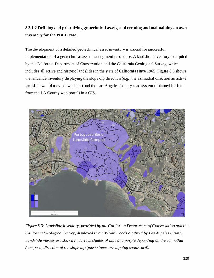
120
8.3.1.2 Defining and prioritizing geotechnical assets, and creating and maintaining an asset
inventory for the PBLC case.
The development of a detailed geotechnical asset inventory is crucial for successful
implementation of a geotechnical asset management procedure. A landslide inventory, compiled
by the California Department of Conservation and the California Geological Survey, which
includes all active and historic landslides in the state of California since 1965. Figure 8.3 shows
the landslide inventory displaying the slope dip direction (e.g., the azimuthal direction an active
landslide would move downslope) and the Los Angeles County road system (obtained for free
from the LA County web portal) in a GIS.
Figure 8.3: Landslide inventory, provided by the California Department of Conservation and the
California Geological Survey, displayed in a GIS with roads digitized by Los Angeles County.
Landslide masses are shown in various shades of blue and purple depending on the azimuthal
(compass) direction of the slope dip (most slopes are dipping southward).

121
8.3.1.3 Assessment and monitor of the performance and health for the assets in the
inventory covering the PBLC, using remote sensing methods, and GIS visualization.
Figure 8.4 shows the average velocity (mm/year) measured across the Palos Verdes Peninsula
between July 2012 and September 2014. Negative values (red) indicate areas of subsidence or
downslope displacements; green values (positive) indicate areas of uplift; yellow values show
regions that are stable. Over 600,000 persistent scatterer (PS) points were obtained, each with
detailed information regarding average velocity, total and incremental displacement, coherence,
and geographic location. Two regions of interest will be investigated: (1) the PBLC and (2) the
city of San Pedro, California.
Figure 8.4: PSI average velocity (mm/year) results over the Palos Verdes Peninsula using 40
COSMO-SkyMed images (July 2012 - September 2014). Average velocity values range from -25
mm/year (subsidence or downslope movements) to 25 mm/year (uplift).
Many separate landslides comprise the PBLC (Figure 8.3). The landslide inventory includes all
landslides that occurred over the past 50 years. In order to determine which slopes are still active
(e.g., are currently moving), the InSAR results from Figure 8.4 were overlaid with the landslide

122
inventory from Figure 8.3. The result and analysis is shown in Figure 8.5. There are four regions
of interest (marked with variegated dashed ovals). The white oval shows a neighborhood entirely
within the PBLC. This portion of the slope appears to be somewhat unstable, with average
velocity values around -5 mm/year and up to -10 mm/year on some buildings. The cyan oval
marks a location where only a few structures, at the end of a cul-de-sac and located within the
previous landslide boundary, experiencing average velocities in the -10 mm/year to -15 mm/year
range. The red oval covers a large portion of the PBLC, near the toe of most of the slopes, where
portions of the slopes are uplifting (green) while other parts of moving downslope (red). Finally,
the magenta oval shows multiple neighborhoods that appear to be moving - at average velocity
rates anywhere between -2 mm/year and -20 mm/year (an order of magnitude!) - but are not
located within any landslide boundary. Combining recent InSAR results with the archival
landslide inventory allows for (1) a determination of which historic landslides are still active and
(2) the location of any unmapped landslides, if any. This remote sensing-based geotechnical
asset management approach enables the monitoring of active slopes (landslides) over the long-
term.

123
Figure 8.5: Average velocity (mm/year) of PS points obtained in the PBLC (July 2012 -
September 2014). Negative values (red) indicate downslope displacement; positive values
(green) indicate uplift.
Another area of interest is San Pedro, California because it is located in what appears to be a
subsidence bowl on the eastern portion of Figure 8.4. A zoomed in image of San Pedro is shown
in Figure 8.6. A total of 71,267 PS points were obtained over San Pedro. A clear subsidence
trend is evident, with average velocities up to -14 mm/year measured in this region. InSAR has
allowed for the detection of this subsidence trend, which can be used to alert mitigation and
construction field crews to the potential damage to transportation and geotechnical assets,
especially near the ‘edges’ of the subsidence trend where the greatest deformation differential is
measured.

124
Figure 8.6: Average velocity (mm/year) of 71,267 PS points obtained over San Pedro (July 2012
- September 2014). Negative values (red) indicate subsidence; positive values (green) indicate
uplift.
Successful implementation of a remote sensing-based geotechnical asset management approach
requires relevant software (e.g., GIS and other software required for data processing), training
for the staff, and resources to review and update asset inventories and life-cycle conditions
throughout the transportation network. This regional approach, as shown using InSAR to identify
locations of greatest asset deterioration, is a great first step towards a multi-tiered geotechnical
asset management procedure.
The next section shows a hypothetical case for retaining walls located along the M-10 highway
in southeastern Michigan - a more local-scale geotechnical asset management approach.

125
8.3.2 Retaining wall asset management example: Hypothetical case for the M-10 site
The study case for the M-10 highway presented in chapters 4 and 5 will be used as a hypothetical
example in this section, to illustrate how the different components of the geotechnical asset
management system could be implemented, focusing on the remote sensing monitoring
techniques.
8.3.2.1 Defining geotechnical asset management system goals for the M-10 Highway case,
and aligning them with the general goals and objectives of the transportation agency.
The agency in charge of the M-10 Highway transportation corridor is the Michigan Department
of Transportation, and they define a comprehensive set of goals, objectives and performance
measures, as part of their strategic planning (Wilbur Smith Associates, 2006). Goals include
preservation of transportation assets, safety to transportation users, basic mobility, and some
other goals. For this example we could focus on the preservation and safety goals, as they apply
to potential failure of geotechnical assets along the M-10 Highway.
The M-10 Highway transportation corridor includes a wide variety of transportation assets, and
provides meets the transportation needs of a large user population (Cerminaro, 2014).
Geotechnical assets include amongst others, a series of retaining walls, as described in chapter 4,
and by Cerminaro (2014). The main function of the retaining walls is to provide structural
support to the fill material that bounds the depressed highway, and constitutes the terrain for the
adjacent service road. This function would be compromised if such structural support was
lacking. Failure of the retaining walls would compromise the depressed highway (M-10) and the
adjacent service road, and even possibly the neighboring residential areas.
Performance degradation could go from minor deformation that would be unnoticeable to the
common transportation system users, to potentially catastrophic collapse of the wall system,
which would put the users at risk of injury or death. In between the extreme cases there is a wide
range of possible scenarios, from minor traffic interruptions required for repairing the walls and
other assets that may be affected by its performance degradation (e. g. the service road surface

126
smoothness), to total closure of the highway needed for major repairing work. Given the
importance of the M-10 Highway (e. g. traffic volume) and the magnitude of the potential
impacts, it becomes evident that maintaining the functionality of the retaining wall system is in
line with the agency goals, at a high priority. For details on the importance of the M-10 highway
and the potential disruption that a failing retaining wall system could cause see Cerminaro (2014)
and references therein.
8.3.2.2 Defining and prioritizing geotechnical assets, and creating and maintaining an asset
inventory for the M-10 Highway case.
Although the M-10 highway transportation corridor includes a very broad set of transportation
assets, it could be argued that retaining walls, are amongst the most important geotechnical assets
in this corridor. Foundations, pavement subgrade and other geotechnical assets could also be
very important, but for the sake of the example we will only consider the retaining walls.
Although currently the Michigan Department of Transportation lacks a comprehensive inventory
of retaining walls, they recently have moved to develop such an inventory for the whole state.
Such an effort would follow a similar procedure to that of retaining wall inventories that have
been developed for other agencies, e. g. De Marco et al. (2010) and Anderson et al. (2008).
8.3.2.3 Assessment and monitor of the performance and health for the assets in the
inventory covering the M-10 Highway, using remote sensing methods, and GIS
visualization and decision support systems.
Following the multi-tier approach to monitoring and managing geotechnical assets outlined
throughout this report, a first level analysis would require a broad assessment and monitoring of
the entire M-10 highway corridor. The initial assessment would be carried out as part of the
inventory development, and would include visual inspection of the conditions for the different
wall sections along the M-10 corridor. Large scale monitoring at this point could include surface
displacement monitoring through InSAR, as described in chapter 4 for this site.

127
The InSAR monitoring did not yield any significant results for the particular M-10 case that we
are considering, although other sites did show movement in that area. For this reason, other
methods may be necessary for monitoring asset performance. In the case of the M-10 retaining
walls, the identification of the problem came from visual inspection, after excessive wall
movement was observed and reported to the Michigan Department of Transportation. It is
however also possible to apply some of the other remote sensing techniques described in this
report, to identify such potential problems.
Once a possible problem has been identified (e. g. excessive retaining wall movement), a more
detailed monitoring is necessary to assess the need for major intervention measures. In the case
of the M-10 retaining walls, the Michigan Department of Transportation applied a series of
traditional surveying methods to track the wall displacement overt time, but some of the remote
sensing techniques described in this report could also have been used. In fact, we applied the
digital photogrammetry method and obtained high quality measurements of the wall relative
displacement, as described in chapters 4 and 5.
The geotechnical asset monitoring information collected through remote sensing and other
methods needs to be processed and analyzed. A GIS based decision support system, like the one
described in chapter 6 could serve for this purpose. Surface displacement information from
InSAR and other sources can be displayed in the GIS interface for the entire M-10 corridor. As
more detailed monitoring is done on specific sites, this information is concentrated in those
areas, with the system allowing to “zoom in” onto the regions of interest.
8.4 Conclusions
The implementation of a geotechnical asset management system requires several important
actions to be taken. Documentation on how to implement transportation asset management
systems have been explored by several authors. AASHTO (2013) describes the process in
general and Vessely (2013) focuses on geotechnical asset management systems in particular;
such work forms the basis for topics discussed in this chapter. Defining the asset management
goals and matching them to the transportation agency’s goals and objectives is key to fully

128
engage the agency in pursuing such a management system. Creating an asset inventory and a
monitoring and performance assessment program for the assets are also necessary steps. The
implementation process needs to be considered in the context of the agency’s limitations and
constraints, and keeping in mind strategies to overcome such limitations and constraints. Some
of the implementation aspects were illustrated with two case study examples, and a more in
depth description of such cases is given in other chapters throughout the report.

129
Chapter 9: Outreach activities
9.1 Introduction
Outreach activities for the project aimed to spread awareness about geotechnical asset
management in general, and the use of remote sensing technologies in particular. After
researching the potential users for such technologies and considering the type of agencies and
companies that would engage in geotechnical asset management, we focused our efforts on
developing multimedia material targeting potential users of the technology. The multimedia
content was designed to match our experience with developing the methods throughout the
project, and we included examples from the fieldwork cases we investigated. Outreach activities
also included direct contact meetings with project partners, to discuss the project’s progress and
their involvement with it.
9.2 Outreach video on remote sensing and geotechnical asset monitoring
To convey the potential use and benefits of using monitoring remote sensing methods for
geotechnical asset management, a video was produce, explaining how the methods work, and the
potential results that can be obtained with them. Video production was done by the Michigan
Tech CinOptic Team. Preparation for video production began in early 2014, through a series of
meeting in which the video’s goals and general content were defined, defined in a strategic
media and outreach plan.
Video footage from fieldwork done as part of the project was collected in July and August of
2014, at the Nevada and Alaska sites. Two CinOptic team members participated in the fieldtrips
and obtained 8 days’ worth of footage of the different aspects of fieldwork, the site conditions,
and the partial results obtained in the field. Other multimedia material collected during the
fieldtrips include photographs, video, interviews and audio captures.
Several individual videos, exploring the specific techniques (i. e. InSAR, LiDAR,
photogrammetry) were produce separately, to address the specific communication needs for each

130
method. Originally the idea was to create a self-contained CD-type product, with a menu for the
individual videos, from which the viewer could navigate and choose what to watch, but this idea
was later change in favor of an on-line version which would not require a CD-reader, and could
be watched in many more platforms. A dedicated YouTube channel was created, and a 7 videos
watch list was uploaded.
The video list opens with an introductory video about sustainable asset management applied to
geotechnical assets. This short video includes interview clips with experts (e. g. Billy D. Connor,
Director of the Alaska University Transportation Center), as well as background footage of the
fieldwork conducted under the project, showing different types of assets. The video can be seen
via this link: https://youtu.be/Qws3quO8fFs
Three videos explain the InSAR, LiDAR and photogrammetry applications to geotechnical asset
management. A video on InSAR technology explains how the use of satellite based InSAR
application can be used to measure very small surface displacements over extensive areas. Clips
from interviews with team members that analyzed the InSAR imagery used in the project, and
who discuss the use of InSAR for geotechnical asset management are presented, with
background videos and animations that illustrate how the methods works. Extensive use of
videos and animations produced by the European Space Agency (ESA) is included in this video
and enhances its visual value, the ESA operates several of the satellites that produce the radar
images that can be used for InSAR monitoring of surface displacements. Clips of the processing
routines were also incorporated in the video. The video can be seen via this link:
https://youtu.be/W-qyvXIIaxU
The LiDAR video also discusses how the technology can be used to monitor geotechnical assets
as part of a geotechnical asset management system. Interviews with team members who worked
on the LiDAR processing and analysis are complemented with field views of the data acquisition
process and animations of how the scanning process works. Videos and animations from third
parties (outside the project) were also used with their permission, to better illustrate some of the
points described in the video. The video can be seen via this link: https://youtu.be/4ealmg_fL2s

131
The digital photogrammetry video follows a similar theme as the two previous videos. The
technique is broadly explained by the team experts who collected, processed and analyzed data
for the project. Videos from the field work and actual videos taken from the acquisition
platforms (e. g. aerial UAV), and are used to illustrate such procedures. Video clips of the data
processing are also included in this video, with a background interview voice explaining some
aspects of the processing. Processing results (e. g. point clouds) are also shown to illustrate the
types of results obtained from the model. This video can be seen via this link:
https://youtu.be/uulqJb9aWBI
To familiarize the viewer with more concrete applications of the methods, two study cases were
summarized and presented in video format as well. A local case study for the M-10 highway
retaining walls study, in Detroit, Michigan, and a regional case study for the southeast Nevada
railroad corridor study. The M-10 Highway retaining wall study focusses on the use of digital
photogrammetry applied to measure surface displacements of retaining walls. Details of the data
acquisition, processing an analysis are given in an interview format, by the team members who
participated in this part of the project. The video makes use of illustrations of the processing,
photographs of the data acquisition, and imagery and videos of the results, using three-
dimensional descriptions of the data that would otherwise be difficult to explain in written or
with two-dimensional figures. The video also includes some examples and results from our
laboratory experiments on scaled models, as they were relevant to this part of the work. The
video can be seen in this link: https://youtu.be/p61b6h0I_zs
The regional case study gives a broader overview of the application of the methods for
monitoring geotechnical assets on a railroad corridor, specifically the potential movement of
rock slopes, as potential precursors to slope instabilities and rock-slides. The video also puts the
methods in the broader context of geotechnical asset management. Interview with project
members who participated in the data collection, processing and analysis are combined with
videos of fieldwork, data processing and results. The video can be seen in this link:
https://youtu.be/fS1u9aIyOCk

132
Finally, a short video with additional interviews of experts and team members, describing the
advantages, potential uses and limitations of the application of remote sensing methods to
geotechnical asset management is also presented, to complement the other videos. Interviews are
combined with fieldwork video and data processing and results illustrations. The video can be
seen here: https://youtu.be/3odYSiQlNmk
Production work for all these videos followed professional standard practices. Extensive
interviewing (several hours total) of experts and project participants was collected and
thoroughly edited to extract only the most informative and relevant clips for the intended content
of the video. To capture the viewers’ attention and give a more pleasant and easy deliverance of
the message content, the editing of the interviews was coupled with field videos and illustrations
of the data acquisition, processing and results, to overlay relevant videos on the interview audio.
Although the audio was entirely based on the interviews, the interviewees appear only for short
periods on screen, alternating this with videos of fieldwork, etc. This visual alternations helps
keep the attention of the viewer and helps to better illustrate the topic being discussed. Figure 9.1
shows a screen capture of two of such editing sessions.

133
Figure 9.1 Screen captures of the video editing process in which interview audio is
combined with fieldwork video.
The videos also make extensive use of other types of illustrations and clips, including those
provided by third parties (e. g. ESA, Riegl, etc.). An effort was made to provide the most
relevant visual illustrations corresponding to the interview topic being discussed in the audio. A
balance between the animations, field or processing videos, and the actual interviewee’s face
being displayed is important, to keep the viewers’ attention focused, but also make this material
personal and understandable. Figure 9.2 shows some screen captures of video illustrations and
interview faces during the editing process.

134
Figure 9.2. Screen captures of different video illustrations for the InSAR video.
The channel with all the videos can be accessed here:
http://mtri.org/geoasset/outreach/
9.3 Outreach activities with project partners
A series of meetings with project partners (Alyeska, Union Pacific, etc.) were held throughout
the project, to inform them on the status of the project, the partial results and to plan joint
fieldwork and data sharing. Figure 9.3 shows a series of slides presented to the Union Pacific
project partners at one of the meetings. This meetings facilitated a two-way exchange of ideas
and a broader discussion of how the results of the project could be applied to geotechnical asset
management. Important input into the projects development by the partners was also
incorporated from these meetings.

135
Figure 9.3. Example of slides from the presentation given to the head of geotechnical engineering at Union Pacific. The slides describe different possible scenarios of slope instability at the Nevada site, and how surface change analysis can help to constrain the likelihood of those scenarios.
Other outreach activities included press releases by Michigan Tech University, that were also
replicated by other parties, e. g. AEG. Figure 9.4 shows a screen capture of a press release by
Michigan Tech University (http://www.mtu.edu/news/stories/2014/october/stabilizing-
geotechnical-assets-new-research-aims-identify-potential-highway-railroad-problems.html), and
the corresponding mention by AEG insider
(http://www.multibriefs.com/briefs/aeg/103014.html).

136
Figure 9.4 Screen captures of a press release by Michigan Tech University (upper panel) that was also feature by AEG insider (lower panel).
9.4 Conference presentations and publications
A series of conference presentations, posters and published articles were also delivered during
the project, and more products like these are expected in the near future. Presentations at
conferences are important to share the projects results with potential users in academia and
industry, and provide an alternative to disseminate the results to a broader audience, who may
not otherwise come across this information, if it was only published as project deliverables and

137
reports. Following is a list of conference presentations and posters, and journal articles on the
project’s results.
Bouali, E.H., Oommen T., Escobar-Wolf R., and Douglas C.S. (2014) An application of
interferometric synthetic aperture radar in a railroad corridor 2014 Annual Technical Forum on
Geohazards Impacting Transportation Aug 6-7, 2014. Lexington, Kentucky.
Cerminaro, D., Oommen T., Escobar-Wolf R., Vitton S., Dobson R.J., Brooks C.N., and Endres
R.B. (2014) Proactive assessment of retaining walls along transportation corridors using optical
remote sensing 2014 Annual Technical Forum on Geohazards Impacting Transportation Aug 6-
7, 2014. Lexington, Kentucky.
Bouali, E.H., Escobar-Wolf R., and Oommen T. (2014) Interferometric synthetic aperture radar
applied to geotechnical asset management in transportation environments 57th Annual Meeting
of the Association of Environmental & Engineering Geologists, Scottsdale, Arizona Sep 20-28,
2014.
Cerminaro, D., Oommen T., Escobar-Wolf R., Vitton S., Dobson R.J., Brooks C.N., and Endres
R.B. (2014) Monitoring retaining walls along transportation corridors using optical remote
sensing 43rd ANNUAL FHWA MIDWEST GEOTECHNICAL CONFERENCE Oct 1-3, 2014.
Bloomington, Minnesota.
Invited talk at the Department of Civil Engineering Seminar, University of Texas, Arlington,
Texas “Sustainable Geotechnical Asset Management Along the Transportation Infrastructure
Environment” (October, 2014)
Invited talk at the Department of Civil Engineering Seminar, University of Michigan, Ann
Arbor, Michigan “Sustainable Geotechnical Asset Management Along the Transportation
Infrastructure Environment” (November, 2014).

138
Cerminaro, D., 2014. Implementation of Photogrammetry to improve proactive assessment of
retaining walls along transportation corridors. Master Degree Thesis (Civil Engineering).
Michigan Technological University. 68 pp.
Justice, S. M. 2015. Application of a hazard rating system for rock slopes along a transportation
corridor using remote sensing. MS Thesis, Michigan Technological University. 89 pp.
Bouali, E.H.Y., Oommen, T., Escobar-Wolf, R.P., 2015, Field verification of satellite-based
velocity data, the 49th annual meeting of The Geological Society of America North-Central
Section Meeting, 19-20 May, Madison, Wisconsin, United States.
Bouali EH, Escobar-Wolf R, Oommen T, 2015, Ground Feature Monitoring Using Satellite
Imagery: How Interferometric Stacking of SAR Can Mitigate Geo-Disasters along
Transportation Corridors, ASCE GEOSTRATA, 2015(4), 38-44.
Bouali EH, Oommen T, Escobar-Wolf R, 2015, Can we extract information regarding
transportation asset condition from satellite-based radar interferometric data? 58th annual
meeting of The Association of Environmental & Engineering Geologists, 19-26 September,
Pittsburgh, Pennsylvania, United States.
Bouali EH, Oommen T, Escobar-Wolf R, 2015, A multi-sensor approach to monitor slope
displacement. American Geophysical Union annual meeting, 14-18 December, San Francisco,
California, United States.
Oommen T, 2015, Sustainable geotechnical asset management along the transportation
infrastructure environment, Van Tuyl Lecture, Colorado School of Mines, October 2015,
Golden, Colorado, USA.
Bouali EH, Oommen T, Escobar-Wolf R, 2016, Interferometric stacking toward geo-hazard
identification and geotechnical asset monitoring, Journal of Infrastructure Systems, 22(2), doi:
10.1061/(ASCE)IS.1943-555X.0000281, 05016001.

139
Bouali EH, Oommen T, Vitton S, Escobar-Wolf R & Brooks C, 2016, Remotely-sensed imagery
and field data used for a Rockfall Hazard Rating System, Environmental and Engineering
Geoscience, under review (submitted February 29, 2016).
Bouali EH, 2016, Monitoring slope instability and ground deformation across the Palos Verdes
Peninsula with COSMO-SkyMed satellite radar imagery, Michigan Technological University
2016 Graduate Research Colloquium, February 24-25, Houghton, MI.
Bouali EH, Oommen T & Escobar-Wolf R: Structure Mapping through Spatial and Temporal
Deformation Monitoring using Persistent Scatterer Interferometry and Geographic Information
Systems. Abstract submitted on March 7, 2016 to present a paper at the 2017 Geotechnical
Frontiers Conference in Orlando, Florida on March 13-16, 2017.
9.5 Project website
A web page with information on the project’s development and progress was also created for
outreach purposes (see figure 9.5). The webpage includes a general project description that
summarizes the original project’s proposal, including the objectives, the planned activities and
the expected outcomes and products. A section on video outreach hosts the videos described in
section 10.2, and a timeline of the project describes how it has been executed. The tasks and
deliverables were also described in detail in one section, to give a more thorough idea of what
the project aims to accomplish. Information on the team members and their email contacts is also
provided, as well as the institutions that they represent. The Technical Advisory Committee is
also listed. Some of the project products (e. g. deliverables) are also displayed and available for
download.

140
Figure 9.5. Screen capture of the home page of the project’s webpage.
The project’s webpage can be accessed here: http://www.mtri.org/geoasset/

141
References
Ahlborn, TM, Shuchman, R, Sutter, LL, Brooks, CN, Harris, DK, Burns, JW, Endsley, KA, Evans, DC, Vaghefi, K, Oats, RC, 2010, An Evaluation of Commercially Available Remote Sensors for Assessing Highway Bridge Condition. Report to the US Department of Transportation, 73 pages. Amekudzi, A., M. Meyer, M. Akofio-Sowah, and R. Boadi (2011). Comprehensive Transportation Asset Management: Making a Business Case and Prioritizing Assets for Inclusion in Formal Asset Management Programs. Technical Report. Georgia Department of Transportation, Office of Materials & Research. 115 pp. American Association of State Highway and Transportation Officials (AASHTO), 1993, Guide for Design of Pavement Structures. AASHTO, GDPS-4, Washington, D.C., 624 pages. American Association of State Highway and Transportation Officials (AASHTO), 2001, Pavement Management Guide. AASHTO, Washington, D.C., 254 pages. American Association of State Highway and Transportation Officials (AASHTO), 2011, Transportation Asset Management Guide, Volume 2: A Focus on Implementation. AASHTO, Washington, D.C., 69 pages. American Association of State Highway and Transportation Officials (AASHTO), 2013, AASHTO transportation asset management guide: a focus on implementation. AASHTO, Washington, D.C., 48 pages. Agisoft, L. L. C., and Agisoft. PhotoScan User Manual. "Professional Edition." Version 1.2. (2016): Agisoft LLC. Anderson, SA, Alzamora, D, DeMarco, MJ, 2008, Asset Management Systems for Retaining Walls. GEO-Velopment: The Role of Geological and Geotechnical Engineering in New and Redevelopment Projects, 162-177. Anderson, SA, Rivers, BS, 2013, Corridor Management: A Means to Elevate Understanding of Geotechnical Impacts on System Performance. Transportation Research Record: Journal of the Transportation Research Board, No. 2349, 9-15. Angeli, M-G, Gasparetto, P, Pasuto, A, Silvano, S, 1989, Examples of landslide instrumentation (Italy). Proceedings of the 12th International Conference on Soil Mechanics and Foundation Engineering, Rio de Janeiro, 3, 1531-1534. Askne, J.I.H., P.B.G. Dammert, and G. Smith, “Understanding ERS InSAR coherence of boreal forests.” Geoscience and Remote Sensing Symposium, 1999, Vol. 4 (1999): 2111-2114. Austroads, 1997, Strategy for improving asset management practices. Austroads Incorporated, Sydney, Australia.

142
Badger, T.C., Fish, M., Trople, T., 2013, Management of unstable slopes along Washington State highways – past, present, and future, Geo-Congress 2013, 1650-1657. Besl, Paul J., and Neil D. McKay. "Method for registration of 3-D shapes." Robotics-DL tentative. International Society for Optics and Photonics, (1992): 586-606. Boardman, A., D. Greenberg, A. Vining, and D. Weimer. (2006). Cost-Benefit analysis. Concept and Practice. 3rd Edition. Pearson / Prentice Hall. 560 pp. Bouali, El Hachemi, Rüdiger Escobar-Wolf, and Thomas Oommen, “Interferometric Synthetic Aperture Radar Applied to Geotechnical Asset Management in Transportation Environments.” (2014) AEG 57th Annual Meeting, Sept 21-27, Scottsdale, AZ. Bouali, El Hachemi, Thomas Oommen, and Rüdiger Escobar-Wolf, “Can we extract information regarding transportation asset condition from satellite-based radar interferometric data?” (2015) AEG 58th Annual Meeting, Sept 20-26, Pittsburgh, PA. Bouali, El Hachemi, Thomas Oommen, and Rüdiger Escobar-Wolf, “Interferometric Stacking toward Geohazard Identification and Geotechnical Asset Monitoring” Journal of Infrastructure Systems, (2016a): 12 p. DOI: 10.1061/(ASCE)IS.1943-555X.0000281. Bouali, El Hachemi, Thomas Oommen, Stanley Vitton, Rüdiger Escobar-Wolf, and Colin Brooks, “Remotely-sensed imagery and field data used for a Rockfall Hazard Rating System” (2016b): under review. Brooks, C., C. Roussi, T. Colling, M. Watkins, B. Hart, D. Dean, J. Garbarino, R. Dobson, and B. White (2013). Deliverable 7-B: Performance Evaluation of Recommended Remote Sensing Systems in Unpaved Road Type Condition Characterization. Michigan Tech Research Institute. 78 pp. Bürgmann, R., P.A. Rosen, and E.J. Fielding. “Synthetic Aperture Radar Interferometry to Measure Earth’s Surface Topography and its Deformation.” Annual Review of Earth and Planetary Sciences, Vol. 28, (2000): 169-209. Calabro, M.D., D.A. Schmidt, and J.J. Roering (2010) An examination of seasonal deformation at the Portuguese Bend landslide, southern California, using radar interferometry. Journal of Geophysical Research, 115, 1-10. Cambridge Systematics, Inc., Applied Research Associates, Inc., Arora and Associates, KLS Engineering, PB Consult, Inc., Lambert, L, 2009, An Asset-Management Framework for the Interstate Highway System. Transportation Research Board, Washington, D.C., 82 pages. Cambridge Systematics, Inc., Parsons Brinckerhoff Quade & Douglas, Inc., Roy Jorgensen Associates, Inc., Thompson, PD, 2002, Transportation Asset Management Guide. American Association of State Highway and Transportation, Washington, D.C., 134 pages.

143
Cerminaro, Daniel J. "Implementation of photogrammetry to improve proactive assessment of retaining walls along transportation corridors." MS Thesis. Michigan Technological University. (2014). 68 pp. Chang, D. Findley, C. Cunningham, and M. Tsai (2014) Considerations for Effective Lidar Deployment by Transportation Agencies. Transportation Research Record: Journal of the Transportation Research Board. 2440, 1-8. Chen, Yang, and Gérard Medioni. "Object modelling by registration of multiple range images." Image and vision computing 10.3 (1992): 145-155. Chou, C, Chen, A, Ling, H, Change, C-M, 2006, Development of the Maintenance Rating Program for City Roadway Networks in Taiwan. Airfield and Highway Pavement Specialty Conference, Atlanta, Georgia, April 30-May 3, 924-935. Connecticut Academy of Science and Engineering (CASE), 2008, Applying Transportation Asset Management in Connecticut. www.ctcase.org/reports/asset_mgmt.pdf Corominas, Jordi. "The angle of reach as a mobility index for small and large landslides." Canadian Geotechnical Journal 33.2 (1996): 260-271. Crosetto, M., O. Monserrat, R. Iglesias, and B. Crippa, “Persistent scatterer interferometry: Potential, limits and initial C- and X-band comparison.” Photogrammetric Engineering and Remote Sensing, Vol. 76, No. 9 (2010): 1061-1069. Cutrona, L.J., “Synthetic aperture radar” in Radar Handbook, second edition, Chapter 21, ed. M. Skolnik, McGraw-Hill, New York (1990). Data Management Association (DAMA), 2009, The DAMA Guide to the Data Management Body of Knowledge (DAMA-DMBOK), First edition. Eds. Mosley M, Brackett, M, Bradley Beach, New Jersey: Technics Publications, 430 pages. DeMarco, M.J., Barrows, R.J., Lewis, S., 2010, NPS Retaining Wall Inventory and Assessment Program (WIP): 3,500 Walls Later, Earth Retention Conference 3, 870-877. Derron, M-H., and M. Jaboyedoff. "Preface" LIDAR and DEM techniques for landslides monitoring and characterization"." Natural Hazards and Earth System Science 10.9 (2010): 1877-1879. Dewberry, (2012). USGS National Enhanced Elevation Assessment. Final Report. 93 pp. Division of Organizational Performance Management (DOPM), 2011, Transportation Asset Management: The strategic direction of Georgia Department of Transportation. www.dot.ga.gov/aboutGeorgiadot/Documents/Asset%20Management/TAM.pdf Dye Management Group, Inc (2009). Transportation Asset Management Feasibility Study. Washington State Department of Transportation. 178 pp.

144
Dzurisin, D. and Z. Lu, “Interferometric Synthetic Aperture Radar” in Volcano Deformation: Geodetic Monitoring Techniques, Chapter 5, ed. D. Dzurisin, Springer-Praxis Publishing Ltd., United Kingdom (2007). Escobar-Wolf, Rüdiger, El Hachemi Bouali, Samantha Justice, Daniel Cerminaro, Thomas Oommen, and Stanley Vitton, “Performance rating of geotechnical assets using remotely measured displacement.” Deliverables 4-A & 4-B USDOT Project RITARS-14-H-MTU, (2015): 48 p. Escobar-Wolf, Rüdiger, El Hachemi Bouali, Thomas Oommen, Daniel Cerminaro, Keith Cunningham, Richard Dobson, and Colin Brooks, “Candidate Remote Sensing Techniques for the Different Transportation Environments, Requirements, Platforms, and Optimal Data Fusion Methods for Assessing the State of Geotechnical Assets.” Deliverable 2-A USDOT Project RITARS-14-H-MTU, (2014): 46 p. Federal Highway Administration (FHWA), 1999, Asset Management Primer. U.S. Department of Transportation, Washington, D.C., 30 pages. Federal Highway Administration (FHWA), 2000, Primer: GASB 34, Office of Asset Management, Federal Highway Administration, Washington, D.C. Federal Highway Administration (FHWA), 2013, Selection Procedure for Reference and Cluster Bridges, http://www.fhwa.dot.gov/multimedia/research/infrastructure/bridges/ltbp/index.cfm Federal Highway Administration (FHWA), 2014, Program Overview, http://www.fhwa.dot.gov/research/tfhrc/programs/infrastructure/structures/ltbp/about.cfm Federico, A, Popescu, M, Elia, G, Fidelibus, C, Internò, G, Murianni, A, 2012, Prediction of time to slope failure: a general framework. Environmental Earth Science, 66, 245-256. Ferretti, A, Prati, C, Rocca, F, 2000, Nonlinear subsidence rate estimation using permanent scatterers in differential SAR interferometry. IEEE Transactions on Geoscience and Remote Sensing, 38(5), 2202-2212. Ferretti, A, Prati, C, Rocca, F, 2001, Permanent Scatterers in SAR Interferometry. IEEE Transactions on Geoscience and Remote Sensing, 39(1), 8-20. Ferretti, A, Fumagalli, A, Novali, F, Prati, C, Rocca, F, Rucci, A, 2011, A New Algorithm for Processing Interferometric Data-Stacks: SqueeSAR. IEEE Transactions on Geoscience and Remote Sensing, 49(9), 3460-3470. Finlay, P. J., G. R. Mostyn, and R. Fell. "Landslide risk assessment: prediction of travel distance." Canadian Geotechnical Journal 36.3 (1999): 556-562. Flintsch, GW, Bryant, Jr., JW, 2006, Asset management data collection for supporting decision processes. U.S. Department of Transportation, Washington, D.C., 97 pages.

145
Florida Department of Transportation (FDOT), 2013, Florida Department of Transportation Maintenance Rating Program Handbook Computer Based Training, http://wbt.dot.state.fl.us/ois/MRPHandbook/index.htm Fukuzono, T, 1985, A new method for predicting the failure time of a slope. Proceedings from the IV International Conference and Field Workshop on Landslides, Tokyo, Japan, 145-150. Galehouse, L, Mouthrop, JS, Hicks, RG, 2006, Principles of pavement preservation. In Pavement preservation compendium II, Federal Highway Administration report no. FHWA-IF-06-049, Washington, D.C., 67-73. Glendinning, S, Hall, J, Manning, L, 2009, Asset-management strategies for infrastructure embankments. Proceedings from the Institution of Civil Engineers, Engineering Sustainability 162, Issue ES2, 111-120. Gutkowski, RM, Arenella, ND, 1998, Investigation of PONTIS – A bridge management software, http://www.mountain-plains.org/pubs/pdf/MPC98-95.pdf, 43 pages. Harvey, M.O., 2012, Optimising road maintenance, International Transport Forum Discussion Paper, No. 2012-12, http://dx.doi.org/10.1787/5k8zvv39tt9s-en, 50 pages. Hawkins, N, Smadi, O, 2013, Use of Transportation Asset Management Principles in State Highway Agencies: A Synthesis of Highway Practice. Transportation Research Board, Washington, D.C., 98 pages. Henriksen, S, 1994, Glossary of the Mapping Sciences. American Society of Civil Engineers (ASCE), New York, NY: ASCE. Hsü, Kenneth J. "Catastrophic debris streams (sturzstroms) generated by rockfalls." Geological Society of America Bulletin 86.1 (1975): 129-140. Huang, SL, Darrow, MM, Calvin, P, 2009, Unstable Slope Management Program: Background Research and Program Inception – Phase I Final Report. Alaska Department of Transportation and Public Facilities, 90 pages. Hunter G, Fell R, 2003, Travel distance angle for “rapid” landslides in constructed and natural soil slopes. Canadian Geotechnical Journal, 40(6), 1123-1141. Jaboyedoff, Michel, Jean-Paul Dudt, and Vincent Labiouse. "An attempt to refine rockfall hazard zoning based on the kinetic energy, frequency and fragmentation degree." Natural Hazards and Earth System Science 5.5 (2005): 621-632. Jaboyedoff, M., and V. Labiouse. "Technical Note: Preliminary estimation of rockfall runout zones." Natural Hazards and Earth System Science 11.3 (2011): 819-828.

146
Jaboyedoff, Michel, et al. "Use of LIDAR in landslide investigations: a review." Natural hazards 61.1 (2012): 5-28. Jansson, P. O. (2013). “Preliminary Findings of Retaining Wall Investigation, W2 of 82-22-12 Northbound M-10 North of Schaefer Highway, City of Detroit”. Michigan Department of Transportation (MDOT), Southfield, MI.- Jenkins, W.S. “Evaluation of Ground-Based Interferometric Radar for Civil Engineering Applications.” Master’s Thesis, University of Missouri-Columbia (2013): 152 p. Justice, Samantha M. “Application of a Hazard Rating System for Rock Slopes along a Transportation Corridor using Remote Sensing”, Master’s report, Michigan Technological University (2015): 86 p. Kilburn, CRJ, Petley, DN, 2003, Forecasting giant, catastrophic slope collapse: lessons from Vajont, Northern Italy. Geomorphology, 54, 21-32. Lee Merkhofer Consulting, 2014, Technical Terms Used in Project Portfolio Management (Continued), http://www.prioritysystem.com/glossary2aa.html Liang, R.Y. “Landslide Hazard Rating Matrix and Database.” Federal Highway Administration, Publication No. FHWA/OH-2007/18 (2007). Lin, Yi, Juha Hyyppä, and Anttoni Jaakkola. "Mini-UAV-borne LIDAR for fine-scale mapping." Geoscience and Remote Sensing Letters, IEEE 8.3 (2011): 426-430. Linder, Wilfried. Digital photogrammetry: theory and applications. Springer Science & Business Media, 2013. Lindquist, K, Wendt, M, 2012, Transportation Asset Management (TAM) Plans including Best Practices: Synthesis. Washington State Department of Transportation, 51 pages. Lowell, S. and P. Morin. “Unstable slope management - Washington state.” Transportation Research News 207 (2000): 11-15. Lucieer, Arko, Steven de Jong, and Darren Turner. "Mapping landslide displacements using Structure from Motion (SfM) and image correlation of multi-temporal UAV photography." Progress in Physical Geography (2013): 0309133313515293. MacDonald, D.B. “Unstable Slopes on I-90 Snoqualmie Pass: Re-assessment and Recommendations.” Washington Department of Transportation (2006). Maerz, N.H., A. Youssef, and T.W. Fennessey. “New risk-consequence rockfall hazard rating system for Missouri highways using digital image analysis.” Environmental and Engineering Geoscience, Vol. 9, No. 3 (2005): 229-249.

147
Massonnet, D, Briole, P, Arnaud, A, 1995, Deflation of Mount Etna monitored by spaceborne radar interferometry. Nature, 375, 567-570. doi: 10.1038/375567a0. Massonnet, D, Rossi, M, Carmona, C, Adragna, F, Peltzer, G, Fiegl, K, Rabaute, T, 1993, The displacement field of the Landers earthquake mapped by radar interferometry. Nature, 364, 138-142. doi: 10.1038/364138a0. Mauldon, M. E. Drumm, W.M. Dunne, V. Bateman, B. Rose, and M. Kim. “Rockfall Management System for Tennessee.” Tennessee Department of Transportation (2007). McDougal, J. (2014). Proposal USGS Broad Agency Announcement for 3D Elevation Program. Southeastern Wisconsin 2015 Regional Lidar and Elevation Data Project. 10 pp. Merriam, R., 1960, Portuguese Bend Landslide, Palos Verdes Hills, California. The Journal of Geology, 68(2), 140-153. Mian, JF, Whittlestone, AP, Patterson, D, Rudrum, DM, 2011, A risk-based approach for the assessment and management of infrastructure assets. Asset Management Conference 2011 IET and IAM, London, United Kingdom, Nov 30-Dec 1, 1-6. Michigan Department of Transportation (MDOT), 2015, Asset Management at MDOT, http://www.michigan.gov/mdot/0,4616,7-151-9621_15757-25283--,00.html Mikkelsen, PE, 1996, Field Instrumentation (Chapter 11). In: Landslide Investigation and Mitigation Special Report 247, edited by Turner AK and Schuster RL. Transportation Research Board, National Academy Press, Washington, D.C., 278-317. Nafaji, M., Salem, S., Bhattachar, D., Salman, B., Patil, R., 2008, An asset management approach for drainage infrastructure and culverts, Project 06-08, June 2008, 271 pages. New York State Department of Transportation (NYSDOT). “Rock Slope Rating Procedure - Geotechnical Engineering Manual.” New York State Department of Transportation, GEM-15 (2007). North Carolina Turnpike Authority (NCTA), 2014, Maintenance Rating Program: Triangle Expressway 2014 Third Quarter Report (July-September), http://www.ncdot.gov/projects/triangleexpressway/download/mrp_q3_2014_final.pdf, 126 pages. Office of Government Commerce (OGC), 2007, Management of risk: guidance for practitioners, 176 pages. Olsen, M., G. Roe, C. Glennie, F. Persi, M. Reedy, D. Hurwitz, K. Williams, H. Tuss, A. Squellati, and M. Knodler. (2013) Guidelines for the use of mobile LIDAR in transportation applications. Transportation Research Board. Vol. 748. 208 pp. Oregon Department of Transportation (ODOT). “Landslide and Rockfall Pilot Study (Final Report).” Oregon Department of Transportation Geo-Hydro Section (2001).

148
Osmanoglu, B. “Synthetic Aperture Radar Interferometry.” Tutorial for Young Scientists offered at the ISPRS TC VII Mid-term Symposium, September 29-October 2 (2014). Pack, R.T. and K. Boie. “Utah Rockfall Hazard Inventory, Phase I.” Utah Department of Transportation, Research Division, UT-03.01 (2002). Pavelka, K., and J. Šedina. (2015). Creating of DSM Based on RPAS Measurement and Accuracy Testing. In Růžičková and Inspektor (Editors) Surface Models for Geoscience. Springer. 316 pp. Peterson, DE, 1987, Pavement Management Practices. NCHRP Synthesis 135, Transportation Research Board, Washington, D.C., 139 pages. Petley, DN, 2004, The evolution of slope failures: mechanisms of rupture propagation. Natural Hazards and Earth System Sciences, 4, 147-152. Petley, DN, Petley, DJ, 2004, On the initiation of large rockslides: perspectives from a new analysis of the Vajont movement record. In: Large Rock Slope Failures, edited by Evans SG, Balkema, Rotterdam (NATO Science Series), 77-84. Pierson, L.A., S.A. Davis, and R. Van Vickle. “Rockfall Hazard Rating System Implementation Manual.” Oregon Department of Transportation, Publication No. FHWA-OR-EG-90-01 (1990). Pierson, LA, 1991, The Rockfall Hazard Rating System. Oregon Department of Transportation, 15 pages. Sahoo, B. C., Oommen, T., Misra, D., & Newby, G. (2007). Using the one-dimensional S-transform as a discrimination tool in classification of hyperspectral images. Canadian Journal of Remote Sensing, 33(6), 551-560. Sanford Bernhardt, KL, Loehr, JE, Huaco, D, 2003, Asset Management Framework for Geotechnical Infrastructure. Journal of Infrastructure Systems, 9, 107-116. Sarmap (2009). Synthetic Aperture Radar and SARscape. SAR-Guidebook. 274 pp. http://www.sarmap.ch/pdf/SAR-Guidebook.pdf Sawtell, Reid, Rüdiger Escobar-Wolf, El Hachemi Bouali, Thomas Oommen, Richard Dobson, and Colin Brooks, “A Review and Demonstration of the Geotechnical Asset Management Decisions Support System (GAMDSS).” Deliverables 5-A & 5-B USDOT Project RITARS-14-H-MTU, (2015) 18 p. Schaefer, L. N., Kendrick, J. E., Oommen, T., Lavallée, Y., & Chigna, G. (2015). Geomechanical rock properties of a basaltic volcano. Frontiers in Earth Science, 3, 29.

149
Schaefer, L. N., Oommen, T., Corazzato, C., Tibaldi, A., Escobar-Wolf, R., & Rose, W. I. (2013). An integrated field-numerical approach to assess slope stability hazards at volcanoes: the example of Pacaya, Guatemala. Bulletin of volcanology, 75(6), 1-18. Schlögel, R, Doubre, C, Malet, J-P, Masson, F, 2015, Landslide deformation monitoring with ALOS/PALSAR imagery: A D-InSAR geomorphological interpretation method. Geomorphology, 231, 314-330. Shan, J. and C. Toth. (2009). Topographic Laser Ranging and Scanning. Principles and Processing. CRC Press. Taylor and Francis Group. 600 pp. Stanley, D. A. (2011). Asset management in a world of dirt: Emergence of an underdeveloped sector of transportation asset management. TR News, (277). Seattle Department of Transportation (SDOT), 2010, Asset Management: Status and Condition Report 2010. www.seattle.gov/transportation/docs/am/CompleteReport0910.pdf Shan, Jie, and Charles K. Toth, eds. Topographic laser ranging and scanning: principles and processing. CRC press, 2008. 600 p. Smith, D. M., Oommen, T., Bowman, L. J., Gierke, J. S., & Vitton, S. J. (2015). Hazard assessment of rainfall-induced landslides: a case study of San Vicente volcano in central El Salvador. Natural Hazards, 75(3), 2291-2310. Stanley, DA, 2011, Asset management in a world of dirt: Emergence of an underdeveloped sector of transportation asset management. TR News 277, 5 pages. Stanley, D.A. & Pierson, L.A., 2012, Performance measures for rock slopes and appurtenances. In Landslides and Engineered Slopes: Protecting Society through Improved Understanding, Proceedings of the 11th International and 2nd North American Symposium on Landslides and Engineered Slopes, eds. E. Eberhardt; C. Froese; A.K. Turner; S. Leroueil, v. 2, 1113-1118. Boca Raton, FL: CRC Press. Stanley, DA, Pierson, LA, 2013, Geotechnical Asset Management of Slopes: Condition Indices and Performance Measures, Special Publication for Geo-Congress 2013: Stability and Performance of Slopes and Embankments III, San Diego, California, March 3-6, 1658-1667. State of Michigan. Center for Shared Solutions. 2013. Lidar Pricings. 1 p. http://www.michigan.gov/documents/cgi/Lidar_Pricing_SOM_CSS_409728_7.pdf Stumpf, André, et al. "Ground-based multi-view photogrammetry for the monitoring of landslide deformation and erosion." Geomorphology 231 (2015): 130-145. United Kingdom Department for Transport (UKDT), 2003, Maintenance of highway geotechnical assets, In Design manual for road and bridges, v. 4, sec. 1, pt. 3. London: UK Department for Transport. www.dft.gov.uk/ha/standards/dmrb/vol4/section1/hd4103.pdf

150
United States Department of Transportation (USDOT), 2005, Recording and Coding Guide for the Structure Inventory and Appraisal of the Nation’s Bridges. Federal Highway Administration, report no. FHWA-PD-96-001, 124 pages. United States Department of Transportation (USDOT), 2007, Asset Management Overview. Federal Highway Administration Office of Asset Management, report no. FHWA-IF-08-008, 52 pages. United States Department of Transportation (USDOT), 2012, Achieving the Bridges of Tomorrow: The Long-Term Bridge Performance Program, publication no. FHWA-HRT-12-017, http://www.fhwa.dot.gov/publications/focus/12sep/12sep03.cfm United States Department of Transportation (USDOT), 2013, Performance Management, http://www.fhwa.dot.gov/map21/factsheets/pm.cfm United States Department of Transportation (USDOT), 2015, Moving Ahead for Progress in the 21st Century Act (MAP-21), http://www.dot.gov/map21 Vermont Center for Geographic Information. 2015. Vermont State LiDAR Plan (10th draft). 11 pp. http://vcgi.vermont.gov/sites/vcgi/files/VT%20State%20LiDAR%20Plan_V10.pdf Vessely, M, 2013, Geotechnical Asset Management: Implementation Concepts and Strategies. United States Department of Transportation, Central Federal Lands Highway Division, Publication No. FHWA-CFL/TD-13-003, 73 pages. Vessely, M. (2013) Risk Based Methods for Management of Geotechnical Features in Transportation Infrastructure. In Geo-Congress. Stability and Performance of Slopes and Embankments III (pp. 1625-1632). ASCE. Vincent, R., and M. Ecker. (2010). Light detection and ranging (LiDAR) technology evaluation Missouri Department of Transportation Technical, Research, Development and Technology. Report No. OR11-007. 104 pp. Voight, B, 1989, A Relation to Describe Rate-Dependent Material Failure. Science, New Series, 243, 4888, 200-203. Wartman, J, Malasavage, NE, 2013, Predicting Time-to-Failure in Slopes from Precursory Displacements: A Centrifuge Experiment. Geo-Congress 2013, 741-749. Westoby, M. J., et al. "‘Structure-from-Motion’ photogrammetry: A low-cost, effective tool for geoscience applications." Geomorphology 179 (2012): 300-314. Williams, K., M. Olsen, G., Roe, and C. Glennie. (2013). Synthesis of transportation applications of mobile LiDAR. Remote Sensing, 5(9), 4652-4692. Wolf, Paul R., and Bon A. Dewitt. Elements of Photogrammetry: with applications in GIS. Vol. 3. New York: McGraw-Hill, 2000. 696 pp.

151
Woodruff, JM, 2005, Consequence and likelihood in risk estimation: A matter of balance in UK health and safety risk assessment practice. Safety Science, 43, 345-353. Yen, K., B. Ravani, and T. Lasky. (2011). LiDAR for Data efficiency. Washington State Department of Transportation. Office of Research and Library Services. Report No. WA-RD 778.1. 101 pp. Yen, K., T. Lasky, and B. Ravani. (2014). Cost-Benefit Analysis of Mobile Terrestrial Laser Scanning Applications for Highway Infrastructure. Journal of Infrastructure Systems, 20(4), 04014022. Zebker, H.A., Werner, C.L., Rosen, P.A., and Hensley, S., 1994, Accuracy of Topographic Maps Derived from ERS-1 Interferometric Radar, IEEE Transactions on Geoscience and Remote Sensing, Vol. 32, No. 4, 823-836. Zerbe, R., and A. Bellas. (2006). A primer for benefit-cost analysis. Edward Elgar Publishing. 316 pp. Zhang, Zhengyou. "Iterative point matching for registration of free-form curves and surfaces." International journal of computer vision 13.2 (1994): 119-152. Zebker, H.A., C.L. Werner, P.A. Rosen, and S. Hensley, “Accuracy of Topographic Maps Derived from ERS-1 Interferometric Radar.” IEEE Transactions on Geoscience and Remote Sensing. Vol. 32, No. 4, (1994): 823-836. Zwissler, B., Oommen, T., & Vitton, S. (2014). A study of the impacts of freeze–thaw on cliff recession at the Calvert Cliffs in Calvert County, Maryland. Geotechnical and Geological Engineering, 32(4), 1133-1148.

152
Appendix: Deliverables:
Available from: http://www.mtri.org/geoasset/tasks/
1-A: Requirements for Remote Sensing Based Geotechnical Asset Management System including Types of Geotechnical Assets and their Conditions that need to be assessed in Different Transportation Environments 2-A: Candidate Remote Sensing Techniques for the Different Transportation Environments, Requirements, Platforms, and Optimal Data Fusion Methods for Accessing the State of Geotechnical Assets 3-A: report “Evaluation of the selected remote sensing techniques to assess the state of geotechnical assets and performance validation with historic geotechnical data” 4-A: A report titled “Performance rating of geotechnical assets using remotely measured displacement” 4-B: A demonstration of how the displacement measured using remote sensing along with other site variables can be used to access the condition of geotechnical assets along the transportation corridor “Performance modeling of geotechnical assets using remote sensing inputs: A geotechnical asset rating tool (GART)” 5-A: A report describing the requirements of the GAMDSS based on project expertise and TAC input, entitled “Geotechnical Asset Management Decision Support System Requirements.” 5-B: A report detailing the GAMDSS software acquired or developed during this project, entitled “A Review of the Geotechnical Asset Management Decision Support System (GAMDSS).” 6-A: Cost benefit analysis of a proactive geotechnical asset management system using remote sensing 7-A: A report titled “An implementation framework of the key project tasks for State DOTs/operators/owners” 7-B: A report describing the specific outreach components completed as part of activity 11, including descriptions of the results identified in the seven-part comprehensive outreach program described in the activity outputs.


