FINAL REPORT Modeling and Simulation of a Distributed Generation-Integrated

Intelligent Microgrid

SERDP Project SI-1650

FEBRUARY 2010

Saifur Rahman Manisa Pipattanasomporn Virginia Tech This document has been approved for public release.

This report was prepared under contract to the Department of Defense Strategic Environmental Research and Development Program (SERDP). The publication of this report does not indicate endorsement by the Department of Defense, nor should the contents be construed as reflecting the official policy or position of the Department of Defense. Reference herein to any specific commercial product, process, or service by trade name, trademark, manufacturer, or otherwise, does not necessarily constitute or imply its endorsement, recommendation, or favoring by the Department of Defense.

Standard Form 298 (Rev. 8/98)

REPORT DOCUMENTATION PAGE

Prescribed by ANSI Std. Z39.18

Form Approved OMB No. 0704-0188

The public reporting burden for this collection of information is estimated to average 1 hour per response, including the time for reviewing instructions, searching existing data sources, gathering and maintaining the data needed, and completing and reviewing the collection of information. Send comments regarding this burden estimate or any other aspect of this collection of information, including suggestions for reducing the burden, to the Department of Defense, Executive Services and Communications Directorate (0704-0188). Respondents should be aware that notwithstanding any other provision of law, no person shall be subject to any penalty for failing to comply with a collection of information if it does not display a currently valid OMB control number. PLEASE DO NOT RETURN YOUR FORM TO THE ABOVE ORGANIZATION. 1. REPORT DATE (DD-MM-YYYY) 2. REPORT TYPE 3. DATES COVERED (From - To)

4. TITLE AND SUBTITLE 5a. CONTRACT NUMBER

5b. GRANT NUMBER

5c. PROGRAM ELEMENT NUMBER

5d. PROJECT NUMBER

5e. TASK NUMBER

5f. WORK UNIT NUMBER

6. AUTHOR(S)

7. PERFORMING ORGANIZATION NAME(S) AND ADDRESS(ES) 8. PERFORMING ORGANIZATION REPORT NUMBER

9. SPONSORING/MONITORING AGENCY NAME(S) AND ADDRESS(ES) 10. SPONSOR/MONITOR'S ACRONYM(S)

11. SPONSOR/MONITOR'S REPORT NUMBER(S)

12. DISTRIBUTION/AVAILABILITY STATEMENT

13. SUPPLEMENTARY NOTES

14. ABSTRACT

15. SUBJECT TERMS

16. SECURITY CLASSIFICATION OF: a. REPORT b. ABSTRACT c. THIS PAGE

17. LIMITATION OF ABSTRACT

18. NUMBER OF PAGES

19a. NAME OF RESPONSIBLE PERSON

19b. TELEPHONE NUMBER (Include area code)

ii

Table of Content

List of Tables ................................................................................................................................. iii  

List of Figures................................................................................................................................ iv  

List of Acronyms .............................................................................................................................v  

Keywords....................................................................................................................................... vi  

Acknowledgement ........................................................................................................................ vii  

1. Abstract........................................................................................................................................1  

2. Objective......................................................................................................................................1  

3. Background..................................................................................................................................3  

4. Materials and Methods ................................................................................................................8  

5. Results & Discussions ...............................................................................................................31  

6. Conclusions and Implications for Future Research ...................................................................47  

Appendix A: Publications..............................................................................................................49  

References......................................................................................................................................50  

iii

List of Tables Table 1. Information sensed and calculated by agents ..................................................................23  Table 2. Control signals from agents.............................................................................................23  Table 3. Various Agents’ Actions in the Collaborative Diagram..................................................26  Table 4. Facts in the IDAPS Multi-Agent System ........................................................................26  Table 5. Requirements to serve non-critical loads during outages................................................43  

iv

List of Figures

Fig. 1. IDAPS cyber-physical system.............................................................................................2  Fig. 2. Distribution circuit of interest .............................................................................................8  Fig. 3. Equivalent circuit of a solar cell..........................................................................................9  Fig. 4. Microturbine model ..........................................................................................................14  Fig. 5. Gas turbine subsystems .....................................................................................................14  Fig. 6. Microturbine model configuration ....................................................................................17  Fig. 7. Part load performance of a 30kW microturbine................................................................18  Fig. 8. Capstone microturbine test – cold start ............................................................................19  Fig. 9. Capstone microturbine test – hot start ...............................................................................19  Fig. 10. Test circuit for the grid connected operation...................................................................21  Fig. 11. PWM controller...............................................................................................................21  Fig. 12. Load control model for an individual load developed in Matlab/Simulink ....................23  Fig. 13. IDAPS agent architecture design and their interaction ...................................................24  Fig. 14. Agent’s collaborative diagram ........................................................................................25  Fig. 15. Middle server implementation........................................................................................30  Fig. 16. PV model.........................................................................................................................32  Fig. 17. The I-V curve from the manufacturer for BP-4175 175W PV module...........................32  Fig. 18. Wind turbine model.........................................................................................................33  Fig. 19. Electrical outputs of wind turbine ...................................................................................33  Fig. 20. Sample outputs of the detailed microturbine model........................................................34  Fig. 21. Sample outputs of the simplified microturbine model ....................................................34  Fig. 22. Load profile of a typical home in summer (August) .......................................................35  Fig. 23. Load profile of a typical home in winter (January).........................................................35  Fig. 24. Test circuit for the grid connected operation...................................................................36  Fig. 25. Simulation result illustrating smooth voltage and current output - grid connected ........37  Fig. 26. Test circuit for the islanded operation.............................................................................38  Fig. 27. Simulation result illustrating smooth voltage and current output - islanded...................38  Fig. 28. The summer TOU rates from the chosen utilities - before demand management...........39  Fig. 29. The summer TOU rates from the chosen utilities - after demand management..............40  Fig. 30. Load profile with agents securing critical loads during the outage between 5-8pm.......41  Fig. 31. The variation of 60Hz voltage and current waveforms...................................................41  Fig. 32. Simulation results during the synchronization of the microgrid to the main grid...........42  Fig. 33. DER output (kW) to serve critical and non-critical loads ...............................................44 Fig. 34. Non-critical load operation (house 1)…………………………………………………..46 Fig. 35. Non-critical load operation (house 2)…………………………………………………..46 Fig. 36. Non-critical load operation (house 3)…………………………………………………..46 Fig. 37. Non-critical load operation (house 4)…………………………………………………..47 Fig. 38. Non-critical load operation (house 5)…………………………………………………..47

v

List of Acronyms AC : Alternating Current

CA : Control Agent DC : Direct Current

DER : Distributed Energy Resources DERA : DER agent

DG : Distributed Generation DOM : Dominion Power

IDAPS : Intelligent Distributed Autonomous Power Systems FIPA : Foundation for Intelligent Physical Agents

IP : Internet Protocol PMSG : Permanent Magnet Synchronous Generator

PLL : Phase Lock Loop PV : Photovoltaic

PWM : Pulse Width Modulation TOU : Time of Use VTES : Virginia Tech Electric Service

UA : User Agent

vi

Keywords

Microgrid, Distributed Energy Resources (DER), Demand Side Management, Multi-Agent System, Renewable Energy

vii

Acknowledgement

We would like to thank the Strategic Environmental Research and Development Program (SERDP) for the financial assistance under Grant no. W912HQ-08-C-0037. Appreciation for technical assistance is extended to Dr. John Hall, Program Manager for Sustainable Infrastructure, and to Carrie Wood, Johnathan Thigpen, and Kristen Lau from HydroGeoLogic, Inc. for their administrative assistance.

1

1. Abstract A reliable, efficient and secure electric power system is necessary for the operation of critical buildings in a base or the whole base itself. This is also applicable for deployed force in forward bases, which have to be put into service quickly and reliably. At present, there is a need to design a distributed and autonomous subset of a larger grid or a microgrid to increase the security and reliability of electricity supply. The objective of this work was to model and simulate a specialized microgrid called an Intelligent Distributed Autonomous Power Systems (IDAPS), which play a crucial role in building a scalable power grid that facilitates the use of renewable energy technologies. Microgrid device models, including distributed energy sources and loads, as well as their control algorithms, were developed. Several case studies were simulated to evaluate the operation of the IDAPS microgrid during parallel and islanded operation modes. Simulation results indicated that the proposed IDAPS control model was able to: (i) perform demand management during normal operating condition; (ii) island the microgrid from the main grid once an upstream fault is detected; (iii) secure critical loads and shed non-critical loads according to the given priority list during emergencies; and (iv) resynchronize the microgrid to the main grid after an upstream fault is cleared.

2. Objective In response to the Statement of Need (SON) NUMBER: SISON-08-04: Scalable Power Grids that Facilitate the Use of Renewable Energy Technologies, we proposed to model and analyze the operation of an Intelligent Distributed Autonomous Power System (IDAPS), which provided the opportunities for load control and dispatch of distributed energy sources, especially renewables. This effort resulted in the intelligent distributed autonomous power grid that could integrate renewable energy technologies and minimize reliance on external energy resources, and thereby reducing fossil fuel consumption. This capability would facilitate the implementation of renewable energy projects and enhance energy security and reliability for the mission-critical parts of military bases and campus-type facilities. In this proof-of-concept, the building blocks of an IDAPS microgrid comprised both physical and cyber systems as illustrated in Fig. 1. The physical system consisted of hardware elements, including distribution circuits, power electronic devices, DERs -- which included both distributed generators and storage technologies -- and loads. DERs in consideration included solar photovoltaics, wind turbines, microturbines, fuel cells, and battery storage technologies. The cyber system consisted of a group of software agents that acted as a central decision support unit. The cyber layer communicated with its associated physical layer through addressable communication interfaces, such as Internet Protocol (IP) addresses.

2

Fig. 1. IDAPS cyber-physical system

During normal operating conditions, the IDAPS microgrid runs in parallel with the local utility. At the same time, it optimally coordinates internal loads, distributed energy resources (DERs) including generation and storage devices to address any operational, environmental, economic, or security constraints. In the event of an upstream outage, the microgrid’s control architecture was designed to isolate the microgrid from the local utility. In such a situation, the microgrid performs load control and activates its internal generators to secure critical loads based on a given prioritized list.

Specifically, the objective of this research was to build a simulation-based model of an IDAPS microgrid. Specific tasks accomplished included:

Task 1: Development of IDAPS device models; Task 2: Development of local control algorithms to control IDAPS device models; Task 3: Development of an IDAPS energy management system; Task 4: Development of addressable IP-based communication interfaces for connecting IDAPS

device models and IDAPS energy management system; Task 5: Simulation and evaluation of the microgrid in both parallel and islanded operations.

In response to the Statement of Need (SON) NUMBER: SISON-08-04, the proposed proof-of-concept work aimed at designing and evaluating a specialized microgrid to enable the following key characteristics:

• Intelligent: In an IDAPS microgrid, all DER devices and loads were an integral part of the network and could be controlled locally. The intelligent features of an IDAPS microgrid implied its ability to perform look-ahead dispatch and demand side management. In the event of a commercial power outage, the highest priority loads were served, while non-critical loads were shed. This depended upon the given prioritized list, available internal generation and expected outage durations.

3

• Distributed: DERs are dispersed in nature. The IDAPS microgrid networked and interconnected various DERs through the integration of the IP-based control model. This thus eliminated single point failures by allowing dynamic response of distributed control strategies, thereby increasing robustness of the local electric power system.

• Autonomous: The IDAPS microgrid was designed to disconnect itself from the local distribution utility and operate autonomously once an outage was detected. The isolation of the IDAPS microgrid from the utility prevented any possible cascading failure. More importantly, it ensured the continuous operation of mission-critical facilities.

• Plug & Play and Scalable: Each physical element in the IDAPS microgrid was assigned a unique IP address. This allowed all DERs and loads to communicate their operational parameters with the system controller. As a result, the current configuration of the IDAPS microgrid could always be updated when additional generators and/or storage devices were added, removed or relocated. Furthermore, since each IDAPS microgrid was modular in nature, several IDAPS microgrids could be interconnected and configured such that they could be the building blocks for a more resilient regional electric power system.

The criteria for success included the demonstration that the proposed microgrid could: (i) perform demand management during normal operating condition; (ii) island the microgrid from the main grid once an upstream fault is detected; (iii) secure critical loads and shed non-critical loads according to the given priority list during emergencies; and (iv) resynchronize the microgrid to the main grid after an upstream fault is cleared. This proof-of-concept work would lay a solid groundwork to gather background information on developing device models within a microgrid, and defining its distributed control environment. It is possible to extend the modeling and simulation based on this work to explore the feasibility of microgrid development in a campus-type facility. The developed simulation platform with some modifications could be used to simulate and analyze the impact of deploying certain types of distributed generation and load control algorithms within a microgrid. Therefore, this makes it possible to quantify and analyze the risks and the impact of various generation and load options before the actual field implementation.

3. Background

3.1 SERDP Relevant

Within the DoD and the new Army Energy Strategy for Installations, one of the major objectives is to decrease dependence on fossil fuels and increase energy security http://army-energy.hqda.pentagon.mil/programs/plan.asp. To achieve this objective, it is necessary to diversify DoD current use of the local electric utility by integrating various types of distributed energy sources, including renewable energy systems such as wind, solar, and other advanced non-polluting Distributed Energy Resource (DER) technologies (e.g., fuel cells and microturbines).

4

At present, the renewable energy integration into the electric power grid only allows parallel operation with no capability to provide power to critical mission facilities during a commercial power outage. To overcome this problem, it is possible to network these power systems together in a scalable intelligent power grid, generally known as a microgrid. Microgrids have emerged as a promising new means to integrate various DERs, together with smart load control strategies, with the aim to increase the resiliency, security, flexibility and efficiencies for the mission-critical parts of military bases and certain campus facilities.

3.2 Previous Work

Discussed below is previous and related work related to microgrid research, development of DER models, together with their control and communication architecture.

3.2.1 Microgrid R&D A microgrid comprises the interconnected distributed generation (PV, wind, diesel, microturbines, fuel cells, etc) – along with energy storage devices (conventional batteries, hydrogen storage, flywheels, etc) – and controllable loads at low-voltage distribution levels. Such systems can operate in parallel with the local utility or in an islanded mode during emergency conditions. Microgrid is one of the key technologies recommended by policy makers drafting technology roadmaps for electricity delivery in many countries, including the United States [1, 2], the European Union [3] and Japan [4]. Subsequent studies have all promoted the microgrid concept citing the increased reliability and power quality it provides to the local utility. At the time of writing this report, there were two major efforts for microgrid development: CERTS/Sandia Labs Microgrid Test Bed [5] and US Army CERL/Sandia Labs Energy Surety Project [6]. The former developed the microgrid test-bed demonstration with American Electric Power. The test-bed comprised three low voltage feeders at 480V and a couple of distributed generators [7]. The work was very comprehensive and covered many aspects of generator controls and parallel operation of various distributed energy sources. The latter addressed the Energy Surety Microgrid project. It was one of the very few reported work that focused on microgrid development at a military base with the objective of creating analytical tools and a methodology to evaluate the impact of infrastructure disruption on base missions [8].

The main challenge identified in microgrid-related research was how to intelligently control and coordinate various DERs to take advantage of their inherent scalability and robustness features. In order to simulate, analyze and evaluate such a feature, building blocks of a microgrid were developed, including models for distributed energy sources and the microgrid control algorithms based on multi-agent technology. Previous and related work related to these topics is discussed below.

3.2.2 Models for Distributed Energy Sources a) Solar PV model Solar Photovoltaic (PV) is a technology that converts sunlight directly into electrical energy. The output is direct current. The major components of a PV system comprise a PV array, a battery storage unit, an inverter and a charge controller.

5

Previous work that developed solar PV models included the following publications [4-12]. Modeling techniques of PV panels were classified into two types: numerical techniques and analytical techniques. The former required iterative processes and mathematical tools to solve the implicit exponential equation associated with diode and photovoltaic devices. The latter involved more simplified and approximated processes; yet was proven to be accurate without introducing significant errors. A very good numerical technique was published in [9] that predicted performance of a solar photovoltaic generator in various operating conditions. Many subsequent publications had also followed this similar method [10, 11, 12, 13, 14]. Accurate analytical methods for the extraction of solar cell model parameters were proposed in [15, 16]. Along this same line, Analytical techniques to determine parameters of solar cells were proposed in [17]. b) Wind turbine model

A wind turbine is used to convert power in the wind into electricity. Main components of a wind turbine generator are turbine blades and a rotor, a gearbox and an electrical generator. Turbine blades convert power in the wind into mechanical power (torque) that is transmitted to a generator via a low-speed shaft, gearbox and a high-speed shaft. The output of a wind turbine can be a DC source, an AC source or a variable frequency AC source, depending on generator types. A power converter is required to connect a wind generator to a utility grid.

The modeling and control of wind turbine for power systems were described in many previous publications [13-16]. The modeling requirements of wind turbine for a power system were investigated and simulated by [18]. The wind turbine model and its performance, linearization and control were presented by [19]. A mathematical and dynamic model of a wind turbine with a doubly-fed induction generator for grid connection was presented by [20]. A dynamic model of a variable speed wind turbine with permanent-magnet synchronous generator to be connected to the grid was developed in Matlab/Simulink by [21]. By integrating the state-of-the-art modeling and simulation, Matlab/Simulink offered a dynamic wind turbine model along with its associated asynchronous generator. c) Microturbine model

Microturbines are small combustion turbines that produce between 25kW and 500kW of power. Microturbines have a common shaft on which is mounted a compressor, a turbine and a generator. These components are mounted on air bearing, thus eliminating friction and maintenance costs. Microturbines have high rotating speeds of 60,000 to 120,000 rpm.

In many previous works, a typical microturbine model was developed by connecting a gas turbine model to a permanent magnet synchronous generator (PMSG) model. The mathematical representations of a heavy-duty gas turbine model were proposed by [22]. The model was suitable for use in dynamic power system studies and in dynamic analyses of connected equipment. Based on Rowen’s model, authors in [23] conducted field tests to derive model parameters and validated the model’s behaviors with actual field data using various types of gas. Subsequently, the proposed heavy-duty combustion turbine model by Rowen was widely used as a gas turbine section of the microturbine simulation model proposed by [24, 25, 26, 27]. In these work, the circuit models of the permanent magnet synchronous generator were developed using the rotor reference frame (dq) for predicting the PMSG’s transient behavior.

d) Fuel cell model

6

Fuel cells are electrochemical energy conversion devices that convert chemical energy in fuel (H2 and O2) into electrical energy. By products of fuel cells are water and heat. A fuel cell comprises two electrodes (anode and cathode) separated by an electrolyte. Fuel (H2) is fed to the Anode. Oxidant (O2) is fed to the Cathode. Power is produced by passing of ions formed at one end to the other end of electrodes. Mathematical and dynamic models of fuel cells were described in many papers [46-49]. A dynamic electrochemical model of the PEMFC along with the simulations and validation results were presented by [28] that showed fuel cell dynamics as well as its power generation. A mathematical model of PEM fuel cells was presented by [29], which also considered the dynamic response of the fuel cells in terms of their transient and thermal properties. A mathematical model of PEM fuel cells, together with their control architecture and a power conditioning system, was presented by [30]. A dynamic Simulink-based model with validated results in both steady and transient states was presented by [31]. Furthermore, Matlab 2008a already implemented generic hydrogen fuel cell stack model, which represented any user-defined fuel cells. e) Battery storage model

Batteries are used to store excess electrical energy from the generation sources and supply the load during the times when the sources are not available. Batteries are charged when an external potential is applied to the batteries’ terminals. Batteries are discharged when an external load is connected to the batteries’ terminals. When batteries are discharged, the batteries’ chemical reaction is reversed and the absorbed energy is delivered. Many battery models were developed over past years [32, 33]. A Thevenin equivalent mathematical battery model was developed by [34]. A kinetic battery model composed of capacity and voltage models was developed by [35] which represents the sensitivity of storage capacity to the rate of discharge. Several other battery models [36, 37] were developed based on the physical and electrochemical processes. Based on some of these previous works, a complete battery model developed by [38] available in Matlab/Simulink comprised a controlled voltage source and an internal resistance with current discharge characteristics.

3.2.3 Multi-Agent Systems for Microgrid Control and Communications A multi-agent system is a combination of several agents working in collaboration in pursuit of accomplishing their assigned tasks to achieve the overall goal of the system. According to [39, 40, 41], a software program was declared as an agent if it exhibited the following characteristics:

• Interacting with the environment and other agents

• Learning from its environment • Reacting to its environment in a timely manner

• Taking initiatives to achieve its goals, and • Accomplishing tasks on behalf of its user

These properties signified the importance of a multi-agent system in developing complex systems that enjoy the agent’s properties of autonomy, sociality, reactivity and pro-activity [42]. Multi-agent systems are being applied in many systems today. Applications of agent-based systems can be divided into single-agent systems, and multi-agent systems. The applications of

7

the former include situations where a human may require assistance while using a computer software. These are, for example, information retrieval and filtering software, meeting scheduler software, mail management engine, news filtering engine, and search engine. The latter is where multiple agents work together to achieve a particular goal. Examples include traffic monitoring systems, decision support systems, manufacturing systems, telecommunications and network management systems, aircraft maintenance, military logistics planning, and power systems.

In general, multi-agent systems were proposed for application in military systems [43, 44, 45], information retrieval systems [46], decision support systems [47], supply chain [48], transportation [49], communication systems [50] and many more [51, 52, 53, 54, 55]. In the context of power systems, multi-agent technologies were applied in a variety of applications, such as to perform power system disturbance diagnosis [56], fault diagnosis [57], power system restoration [58], power system secondary voltage control [59] and power system visualization [60]. The multi-agent systems for power engineering applications were discussed in [61,62]. The distributed control approach was implemented in [63] using multi-agent systems technology. In [64, 65,66], the authors implemented multi-agent systems for optimal operation of microgrids. In [67], a multi-agent system was proposed that attempts to restore a distribution system network after a fault.

3.3 Proof of Concept and its Technical Challenges

This work focused on modeling and simulation of a microgrid that networked variety of distributed energy sources. Key technology gaps addressed included the development of a distributed agent system that controlled and networked distributed energy sources, as well as analyzing the dynamic response of distributed control strategies. In a given situation, an agent must be able to issue a control signal in response to an event sensed from the external environment quickly enough to manage the microgrid in a timely fashion. The simulation and evaluation case studies were conducted to test network interoperability in both on- and off-grid operation. As previously discussed in Section 2, our success criteria were to demonstrate that the proposed microgrid could: (i) perform demand management during normal operating condition; (ii) island the microgrid from the main grid once an upstream fault is detected; (iii) secure critical loads and shed non-critical loads according to the given priority list during emergencies; and (iv) resynchronize the microgrid to the main grid after an upstream fault is cleared. Through the development of a “plug-and-play” interconnected power grid, it is expected that this work can contribute to allowing the installation or deployed force to: (1) install future renewable energy systems and (2) effectively control and optimally benefit from the power that is generated from DERs. The power grid should provide these capabilities during both normal grid-connected and emergency or islanded operating conditions.

8

4. Materials and Methods

4.1 Task 1: Development of IDAPS Device Models

A) Task Description Task 1 involved the development of IDAPS hardware models using the SimPowerSystems toolbox in the Matlab/Simulink environment. IDAPS hardware components included distribution circuit, distributed energy resources (DERs) and loads. DERs of interest included solar photovoltaic modules, wind turbines, microturbines, fuel cells and battery storage. Below are the descriptions of how the model of each physical element in the IDAPS microgrid was developed.

B) Distribution Circuit The models of distribution circuit components, including circuit breakers, transformers and lines, were readily available in the SimPowerSystems libraries. These existing models were used, together with the system parameters from Virginia Tech Electric Services (VTES), to build a simplified distribution circuit, as shown in Fig. 2. System parameters needed to construct the distribution circuit in Matlab included system voltage, the length of the line, line resistance and reactance, transformer size and the circuit topology.

Fig. 2. Distribution circuit of interest

C) Distributed Energy Resources (DERs) Description of the development of each model is summarized below.

9

C.1) Model of Solar PV Modules a) Model Description

The model of a solar photovoltaic (PV) generator was developed in the Matlab/Simulink environment. It was designed such that standard electrical characteristics of solar cells, as well as temperature and solar irradiation were used as inputs. The standard electrical characteristics used as inputs to the model included: open-circuit voltage (Voc), number of cells connected in series (Ns), short-circuit current (Isc), number of cells connected in parallel (Np), maximum module power (Pmax), temperature coefficient of open-circuit voltage and temperature coefficient of short-circuit current. These parameters could be obtained from a manufacturer’s datasheet. Additional inputs to the model were cell temperature and solar irradiation, which could be obtained from historical data. Model outputs were PV outputs, including voltage and current, at the maximum power point.

b) Mathematical Formulae The equivalent circuit of a photovoltaic cell is represented by a constant current source (Iph) connected with a diode and a series resistance (Rs,cell), as shown in Fig. 3.

Fig. 3. Equivalent circuit of a solar cell

The net cell current (Icell) can be determined by subtracting the diode current (Id) from the photo-generated current (Iph) as follows.

€

Icell = Iph − Id = Iph − I0 expq(Vcell + IcellRs,cell )

mkTc−1

⎛

⎝ ⎜

⎞

⎠ ⎟ (Eq. 1)

where Icell = net cell current

Vcell = cell voltage Iph = photo-generated current which depends on solar irradiation

I0 = diode dark satulation current q = Magnitude of electron charge (1.6x10-19)

k = Boltzmann’s constant (1.38x10-23) m = 1-2, a constant depending on material and physical structure of a solar cell

Tc = absolute cell temperature (K) Let Vt,cell = mkTc/q, representing a cell thermal voltage. With the assumption that the photo-generated current (Iph) equals the short-circuit current (Isc,cell) and exp(q(V+IRs)/mkTc) >> 1 under all working conditions, Eq. 1 can be rewritten as:

+

V

-

10

€

Icell = ISC ,cell − I0 expVcell + IcellRs,cell

Vt,cell

⎛

⎝ ⎜

⎞

⎠ ⎟ (Eq. 2)

Considering an open-circuit condition, the open-circuit voltage can be determined from Eq. 2 given the solar cell generates no current (Icell = 0) as:

€

VOC ,cell =Vt ,cell lnISC ,cellI0

⎛

⎝ ⎜

⎞

⎠ ⎟ (Eq. 3)

As a result, I0 can be expressed as a function of Isc as:

€

I0 = ISC ,cell exp −VOC ,cellVt,cell

⎛

⎝ ⎜

⎞

⎠ ⎟ (Eq. 4)

By substituting I0 from Eq. 4 into Eq. 2:

€

Icell = ISC ,cell 1− expVcell −VOC ,cell + IcellRs,cell

Vt,cell

⎛

⎝ ⎜

⎞

⎠ ⎟

⎛

⎝ ⎜ ⎜

⎞

⎠ ⎟ ⎟ (Eq. 5)

Eq. 5 represents the relationship between the cell current and the cell voltage in terms of short-circuit current, open-circuit voltage, as well as series cell resistant and cell temperature. A PV module consists of many solar cells connected in series and parallel in order to generate a required open-circuit voltage or short-circuit current. Similarly, a PV generator consists of many PV modules. By assuming that every solar cell constituting a PV module or a PV generator are identical and has the same operating characteristic under the same illumination and temperature, the characteristic I-V curve for a PV module or a PV generator can be derived by considering that:

€

IModule = Icell ⋅ Np (Eq. 6)

€

VModule =Vcell ⋅ NS (Eq. 7)

Where IModule and VModule respectively are the current and voltage of a PV module. Np and Ns are the number of cells connected in parallel and series that make up a PV module. IModule and VModule can also represent the current and voltage of a PV generator when Np and Ns represent the number of cells connected in parallel and series that constitute a PV generator. Using Eq. 6 and Eq. 7, Eq. 5 can be rewritten to represent the relationship between the module current and the module voltage as:

€

IModule = NpISC ,cell 1− expVModule − NsVOC ,cell + IModuleRs,cell (Ns /Np )

Ns ⋅Vt ,cell

⎛

⎝ ⎜

⎞

⎠ ⎟

⎛

⎝ ⎜ ⎜

⎞

⎠ ⎟ ⎟ (Eq. 8)

This is the key equation that will be used to derive the I-V curve of a PV generator. Most parameters on the right-hand side of the above equation (VOC,cell@STC, ISC,cell@STC and Pmax,cell@STC) are readily available from manufacturer’s datasheet.

11

The cell series resistance (Rs,cell) is a property of the solar cells, and must be determined at the standard test condition (STC). This value is assumed to be unaffected by temperatures and solar illumination. The cell series resistance can be derived using the following relationships:

€

Rs,cell = 1− FFSTCFF0STC

⎛

⎝ ⎜

⎞

⎠ ⎟ ×

VOC ,cell@ STC

ISC ,cell@ STC

(Eq. 9)

where:

VOC,cell@STC = Voc,module / Ns ISC,cell@STC = Isc,module / Np

Pmax,cell@STC = Pmax,module / (Ns Np) FFSTC = Pmax,cell@STC / (VOC,cell@STC x ISC,cell@STC)

FF0,STC = (vocSTD – ln(vocSTD + 0.72))/(vocSTD + 1) Where vocSTD is normalized voltage at the standard test condition:

vocSTD = VOC,cell@STC / [k (273+Tc) / q]

Derivation of VOC,cell and ISC,cell at an Operating Condition Some adjustments are necessary to modify open-circuit voltage and short-circuit current, which are given at the standard test condition, to an operating condition at a particular irradiation and temperature level.

It is generally assumed in practice that the short-circuit current of a solar cell depends linearly and exclusively on solar irradiation. In addition, the short-circuit current of a solar cell increases with the cell’s temperature. Most manufacturer’s datasheet gives this information in terms of a short-circuit temperature coefficient (A/°C).

€

ISC ,cell = ISC ,cell@ STCGGSTC

⎛

⎝ ⎜

⎞

⎠ ⎟ +α Tc −TSTC( ) (Eq. 10)

Where:

G = solar irradiation (W/m2) GSTC = solar irradiation at the standard test condition (W/m2)

α = temperature coefficient of short-circuit current (A/°C)

Tc = cell temperature (°C)

TSTC = cell temperature at the standard test condition (°C)

The open-circuit voltage of a solar cell decreases with the cell’s temperature. Manufacturer’s datasheet generally gives this relationship in terms of a constant C3 (V/°C). In addition, the open-circuit voltage increases slightly with irradiation according to the following relationship.

12

€

VOC ,cell =VOC ,cell@ STC +mkTcq

ln GGSTC

⎛

⎝ ⎜

⎞

⎠ ⎟ + β(Tc −TSTC ) (Eq. 11)

Where: β = Temperature coefficient of open-circuit voltage (V/°C)

C.2) Model of Wind Turbines a) Model Description:

This study used the previously developed wind turbine model in Matlab as a basis for the simulation study. In this case, the wind turbine generator was modeled as a wind turbine section connected with an electrical generator section. The turbine section was modeled based on the steady-state power characteristics of the turbine and required as inputs: (1) the generator speed in per unit of the nominal speed of the generator, and (2) the wind speed in m/s. Output of the turbine block was the mechanical torque (Tm) in per unit of the nominal torque of the generator that applied to the generator shaft. The mechanical torque was used as an input to the asynchronous generator. The output of the wind turbine model was the three-phase power that could be directly connected to the electrical grid. b) Mathematical Formulae

Eq. 12 describes the relationship between the mechanical power output (watts) of a wind turbine and the wind speed in m/s.

€

Pm = cp λ,β( ) ρA2υ 3 (Eq. 12)

Where Pm : Mechanical output power of the turbine (Watts) Cp : Performance coefficient of the turbine β : Blade pitch angle (degree) λ : Tip speed ratio of the rotor blade tip speed to wind ρ : Air density (kg/m3) A : Turbine swept area (m2) ν : Wind speed (m/s)

Cp represents extractable power from the wind. Cp is a function of blade pitch angle (β) and tip speed ratio (λ). Maximum possible Cp is 0.5928, according to Betzz limit. In this study, we shall use a generic equation of Cp as proposed by [68], which is expressed according to the following formula.

€

cp λ,β( ) = 0.5176 116λi

− 0.4β − 5⎛

⎝ ⎜

⎞

⎠ ⎟ ⋅ e

−21λi + 0.0068λ (Eq. 13)

Where:

€

λi =1

λ + 0.08β−0.035β 3 +1

⎛

⎝ ⎜

⎞

⎠ ⎟

−1

13

According to the above equations, the maximum possible performance coefficient of a turbine is 0.48 (Cpmax = 0.48) and is achieved for β = 0° and tip speed ratio λ = 8.1. This value will be defined as the nominal value (λnom). It is interesting to note that, at a constant tip speed ratio, i.e. λ = 8.1, increasing blade pitch angle will result in lower performance coefficient (Cp), thus reducing the turbine power output.

Note that the tip speed ratio λ is a ratio of rotor speed to wind speed. This rotor speed is equivalent to the generator speed because the turbine rotor and the generator are connected via a gearbox. Eq. 13 implies how faster the blade can rotate as compare to the wind speed.

€

λ =2πR rpm

60υwind

(Eq. 14)

where R : Blade radius (meters), i.e. 40m for a 2MW V80 turbine νwind : Wind speed (m/s) rpm : Blade speed (rpm), i.e. 9-19rpm for a 2MW V80 turbine

The detail of asynchronous generator model was well documented in Matlab/Simulink and would not be discussed in further detail here.

C.3) Model of Microturbines Two types of microturbine models were developed, namely (a) the detailed model and (b) the simplified model. The detailed model was developed to study the real-time system interaction (in millisecond timeframe). However, the simulation time to run the detailed model was significantly long. To reduce the simulation time, the simplified model was developed to enable the study of the IDAPS energy management system for a 24-hour period.

C.3.1) The detailed microturbine model a) Model Description:

According to [69], a microturbine model comprised a gas combustion turbine engine integrated with an electrical permanent magnet synchronous generator (PMSG) that produced electric power while operating at a high speed. As shown in Fig. 4, the inputs of the gas turbine sections were per unit turbine speed (output from PMSG) and a rotor reference speed. The gas turbine compared the rotor speed and the reference speed and adjusted its outputs -- per unit fuel flow and per unit turbine torque -- to keep the rotor speed of the PMSM at the reference speed. In addition to the per unit fuel demand and the per unit turbine torque, the other output of the gas turbine section was the exhaust temperature (F).

14

Fig. 4. Microturbine model (Gas turbine subsystem with PMSG)

As shown, torque from the turbine in per unit was converted to Newton-meter (Nm), and then was used as an input to drive the PMSG. Outputs from PMSG were three-phase power and rotor speed (rad/s). The rotor speed (rad/s) was converted to a per unit quantity and was fed back to the turbine section.

b) Mathematical Formulae b.1) The gas turbine section:

The gas turbine section of this model was built according to the mathematical representations of heavy-gas turbines presented in [70]. The block diagram of the gas turbine section is shown in Fig. 5. The validity of the model is limited to simple cycle single-shaft, generator drive gas turbine only.

Fig. 5. Gas turbine subsystems

1) Speed control 2. Fuel control system

3. Compressor-turbine

4. Temperature control

LVG

15

The dynamic model for a combustion gas turbine consisted of the following subsystems: (1) speed control; (2) fuel control; (3) compressor-turbine; and (4) temperature control. All parameters and constants used in the gas turbine model were extracted from [71]. Speed control section: The speed control section compared the current rotor speed (from PMSG) with the reference speed in per unit quantities. The dynamic response of the speed control section was modified by adjusting parameters in the transfer function. The output of the speed control section was one of two inputs to the least value gate (LVG). The other input was from the temperature control section. The lowest value of the two inputs was sent to the saturation block (for a typical gas the minimum and maximum limits are -0.1 and 1.5, respectively) and forwarded to the fuel control system.

Fuel control section: The output from LVG represented the least amount of per unit fuel needed for a particular operating point that corresponds directly to the per unit mechanical power on turbine base in steady state. For example, if mechanical power was 0.7 pu then the steady state value for fuel demand signal was also 0.7 pu. To obtain the final fuel demand signal, the per unit fuel demand from the LVG was multiplied by the per unit turbine speed. The output was then scaled with gain K = 0.77, then offset by the constant 0.23, which represented the minimum amount of fuel flow at no load rated speed. The fuel control system section of the diagram above could be interpreted as follows:

• When no more fuel required (fuel control = 0), fuel demand signal = 0.23. • When fuel control = 1, turbine speed = 0.5, fuel demand signal = 0.23+0.5*0.77 = 0.615. • When fuel control = 1, turbine speed = 1.0, fuel demand signal = 0.23+1.0*0.77 = 1.0.

The fuel control section also consisted of the fuel valve positioner and fuel actuator. The transfer functions associated with valve positioner and fuel actuator generated some time delays, which in this case was modeled at 0.05 and 0.04 seconds, respectively.

Compressor-turbine section: The fuel combustion in the combustor resulted in turbine torque and in exhaust temperature. Inputs of the compressor-turbine section were the per unit turbine speed (N) and per unit fuel flow required (Wf). Outputs of the compressor-turbine section were per unit torque and exhaust temperature (in F), given as inputs. Torque and exhaust temperature related to fuel flow (Wf) and turbine speed (N) linearly according to the following relationships.

Torque = KHHV (Wf – 0.23) + 0.5 (1 - N) (Nm) (Eq. 15)

Exhaust Temp (TX) = Tref - 700 (1 – Wf) + 550 (1 – N) (F) (Eq. 16)

Where:

Wf : per unit fuel flow N : per unit rotor speed

KHHV : coefficient that depends on the higher heating value of the gas stream in the combustion chamber (KHHV = 1.2 for a typical gas)

Tref : Reference temperature (950°F)

16

In the compressor-turbine sections, time delay associated with the combustion reaction, time delay associated with the compressor discharge volume, and a transport delay associated with the transportation of gas from the combustion system through the turbine were set at 0.01 second, 0.2 second and 0.04 second, respectively.

Temperature control section: The temperature control section was designed to limit output power of the gas turbine if the exhaust temperature of the turbine was higher than a pre-determined reference temperature. In practice, the exhaust temperature was measured using a series of thermocouples incorporating radiation shields, both of which were modeled by using transfer functions that resulted in very high time delays. The output of the thermocouple was compared with a reference temperature (950F in this case). If the reference temperature remained higher than the thermocouple temperature, which was usually the case, this would permit the dominance of speed control through the LVG. When the thermocouple output exceeded the reference temperature, the difference became negative and the temperature control output would be lower than the speed control output. This allowed the temperature control signal passing through the LVG and limits the turbine’s output. b.2) Permanent Magnet Synchronous Generator

A permanent magnet synchronous generator is a synchronous generator, in which the DC field winding of the rotor is replaced by a permanent magnet.

The voltage rating of the machine: could be changed by varying the amount of flux induced by magnets. The relationship between flux and generate voltage of the machine used was:

€

Ea = Km ⋅ω(rad /s) (Eq. 17)

Where Km = motor torque constant (Nm/A), which is a function of flux induced by magnet Ea = stator voltage (Vrms/phase)

ω = rotor speed (rad/s)

€

Km =32⋅ p ⋅ϕ (Eq. 18)

p = number of poles

ϕ = flux (Wb)

For example, if we would like to design a PMSG with the voltage rating of 480Vrms (line-line) and the rotor speed of 70,000 rpm, the flux per phase would be 0.008911 Wb/phase.

€

Ea =32⋅ p ⋅ϕ ⋅ω(rad /s)

=32⋅ 2 ⋅ 0.008911⋅ 70000 × 2π

60= 277.1 Vrms / phase or 480 Vrms( l− l )

Power rating of the machine: could be changed by varying the resistance and reactance of the machine. We used typical resistance and reactance values for a synchronous machine of 0.01 per

17

unit and 0.15 per unit, respectively. For example, if we would like to design a PMSG with the power rating of 30kW and the voltage rating of 480Vrms (line-line),

Vbase = 480/sqrt(3) Vrms (line-neutral) Pbase = 30kW

Ibase = 36.1 A Zbase = Vbase/Ibase = 7.68 Ohm

Ra = 0.01x7.68 = 0.0768 Ohm Xa = 0.15x7.68 = 1.152 Ohm

@ 70,000rpm → La = 7.858x10-5 Henry

C.3.2) The simplified microturbine model a) Model Description:

A simplified microturbine model was developed following the characteristics of a 30kW capstone microturbine, in terms of its efficiency and the rise time. As shown in Fig. 6, the model’s input was the microturbine’s power set point that sets the amount of power required from the microturbine. The output of the model was its power output (kW) and the amount of fuel used (BTU or cu ft).

Fig. 6. Microturbine model (Input is power set point; outputs are power output and fuel and

power measurements)

b) Mathematical Formulae (Microturbine’s Efficiency and its Behavior during Load Changes) Efficiency: In general, the efficiency of a microturbine decreases when it is partially loaded. At full load, the efficiency of a typical 30kW microturbine was approximately at 28%. At half load, the microturbine efficiency decreased to approximately 23%. According to the characteristic of a 30-kW microturbine [72], Fig. 7 illustrates the microturbine part load power performance.

18

Fig. 7. Part load performance (black) of a 30kW microturbine and its piecewise linear curve fit

(green) (Source: Energy Nexus Group)

To model this relationship in Matlab/Simulink, the piecewise linear curve was built to fit the part load performance curve. This was also shown in Fig. 7 as a solid green piecewise linear line. The curve fit equations used were as follows:

When the percent load (Li) is less than or equal to 15%, ηi = (2*Li + 0.35) x ηMT

When the percent load (Li) is between 15% and 40%, ηi = (0.8*Li + 0.53) x ηMT

When the percent load (Li) is between 40% and 100%, ηi = (0.25*Li + 0.75) x ηMT

Where: ηI = microturbine efficiency in hour i

Li = load in percentage of microturbine capacity in hour i ηMT = microturbine efficiency at full load of 28%

Rise time: Fig. 8 illustrates the characteristic of a 30kW capstone microturbine when responding to the power demand. Fig. 8 indicates that it took about 40 seconds for a microturbine to increase the power output from zero to full load after receiving the power demand signal. This hot start characteristic was imitated in the simplified microturbine model using a signal generator.

Efficiency

28.0%

22.4%

16.8%

11.2%

5.6%

19

Fig. 8. Capstone microturbine test – cold start (Source: CERT [73])

Start-up time: The start-up characteristic of the microturbine is also illustrated in Fig. 9, which implies that it took about 3 minutes to increase the turbine’s power output to full load from its OFF state. Similar to the cold start characteristic, this hot start characteristic was imitated in the simplified microturbine model using a signal generator.

Fig. 9. Capstone microturbine test – hot start (Source: CERT [73])

C.4) Model of Fuel Cells

20

The fuel cell model available in Matlab/Simulink was used in the simulation. The mathematical formulae for the model development were extensively discussed in Matlab 2009 Documentations and would not be repeated here. C.5) Model of Battery

The battery model available in Matlab/Simulink was used in the simulation. Slight modifications were made internally to the model to ensure that the model could run at the required time step (either one minute, one second or less). The mathematical formulae for the model development were extensively discussed in Matlab 2009 Documentations and would not be repeated here.

D) Load Models This study focused on household loads and their usage characteristics. Hourly residential load curves of an average household used in this study were extracted from the RELOAD database [74], which was used by the Electricity Module of the National Energy Modeling System (NEMS). The hourly residential load curve data were available for twelve months (January to December), three day types (typical weekday, typical weekend and typical peak day) and nine load types (space cooling, space heating, water heating, cooking, cloth drying, refrigeration, freezing, lighting and others). As the load curves in the RELOAD database represented hourly fractions of the yearly load, the load curves were scaled up by the annual household consumption and divided by the number of hours in a year, which is 8760. Therefore, the adjustment made to the hourly RELOAD residential load curves for each load type could be represented by Eq. 19.

€

Lhour = f × Lannual8760

(Eq. 19)

where: Lhour = Average hourly load (kWh/h) f = Hourly fraction of yearly load Lannual = Average annual household load

4.2 Task 2: Development of Local Control Algorithms to Control IDAPS Device Models

A) Task Description Task 2 involved the development of local control algorithms to control DER units, and loads. Particular focus was given to the DER units that require inverter interface with the utility grid.

B) DER Control Local Control during the Grid Connected Mode:

During the grid connected mode, voltage magnitude and phase at the interconnection point were the two control parameters. Voltage magnitude and phase from DER must be compatible with those at the interconnection point to ensure smooth interconnection. The local control circuit is illustrated below that provides the grid interface between a DER device and the utility.

Distributed

generator

Grid interface: Inverter, PWM controller, filter

Loads & measurements

Isolation transformer & the grid

21

Fig. 10. Test circuit for the grid connected operation

As shown, the grid interface section comprises an inverter, a PWM controller and a filter. The PWM controller is responsible for calculating voltage magnitude and phase based on the measurement at the interconnection point (bus B2 in Fig. 10). The outputs from the PWM controller were used to control the output of the inverter so that the output voltage from DER (bus B1 in Fig. 10) was compatible with that at the interconnection point (bus B2) at all time.

The PWM controller comprises a phase-lock loop (PLL) unit and voltage and current regulators (PI controllers). See Fig. 11.

Fig. 11. PWM controller

The following regulator gains were used for the PLL unit and the voltage and current regulators.

22

Proportional gain (Kp)

Integral gain (Ki)

Derivative gain (Kd)

PLL block 60 1400 0

DC voltage regulator block 0.01 3 0

Current regulator block 0.05 (0.5) 2 (5) 0

Local Control during the Islanded Mode:

During the islanded mode, the configuration of the DER control unit used was the same as that during the grid connected mode. In this case, the PWM controller would monitor the voltage magnitude and phase at the interconnection point, and ensure that the DER could connect with the rest of the system. For a system with a single inverter-based DER, the PWM setting would be set to follow the reference voltage at 1 per unit and the frequency of 60 Hz at all time.

C) Load Control

Load control strategies were designed based on load types. In this study, household loads were classified into three groups, namely critical, interruptible and deferrable loads.

• Critical loads were defined as loads that should not be shut down or shed even during emergency condition.

• Deferrable loads were referred to as the loads that could be shifted to operate during the later hours during shortages or high electricity price periods. These loads may include water heating, clothes washing, clothes drying and other plug-in loads.

• Interruptible loads were defined as the loads that could be curtailed during emergencies or during the high electricity price periods. These loads may include space cooling and optional lighting loads.

The load control strategy was developed as a generalized load control model for each individual load as shown in Fig. 12.

23

Fig. 12. Load control model for an individual load developed in Matlab/Simulink

As shown, the model required the followings as inputs: (1) price signal or emergency signal from external sources; (2) the load profile; (3) percentage of allowable demand reduction, for example, this number is 0% for critical loads and is 100% for interruptible loads; and (4) percentage of compensation after deferring the load, for example, this number is 0% for critical loads and is 100% for interruptible loads.

4.3 Task 3: Development of an IDAPS Energy Management System

A) Task Description This task involved the development of the IDAPS energy management system based on a multi-agent technology. This section defines the environment in which the IDAPS agents resided, the IDAPS agent architecture -- which included types, roles and their interaction -- and lastly the IDAPS agent decision criteria during normal operation and outage durations.

B) Defining the Agent Environment In an IDAPS microgrid, the agents interact with the environment through sensors and actuators. Sensors provide agents with the current status of the microgrid, while actuators activated, controlled, or inactivated a process or action. In the system under study, IDAPS agents require sensors to sense the following information from various devices.

Table 1. Information sensed and calculated by agents

Device/system Information Sensed Information calculated DERs Magnitude and phase of voltage and

current outputs Power output (kW), fuel used (gallons or BTUs), emission produced (lbs)

Battery Voltage, charge/discharge current, state of charge

Power charged or power discharged (kW)

Loads Magnitude and phase of voltage and current consumed at the load

Power consumed (kW)

Switches Status ON/OFF N/A Utility system Electricity price ($/kWh) – the price

can vary from every minute to every hour; system frequency and voltage

Whether or not the system’s voltage and frequency are in the safe operation range

Agents issue the following control signals to control each device in the IDAPS microgrid.

Table 2. Control signals from agents

Device/system Control signals from agents DERs Power set point Battery Charge/discharge signal Loads Status ON/OFF, consumption reduction

24

Switches Status ON/OFF Utility system Disconnect the microgrid once an upstream failure is detected.

C) Defining the Agent Architecture (Type, Role, Interaction) Defining Types of Agents:

In this study, the idea behind any multi-agent system is to break down a complex problem handled by a single entity into smaller simpler problems handled by several entities. This is called a distributed and decentralized system. The proposed multi-agent system consisted of four agents, namely control agent, DER agent, user agent and database agent. The four agents together formed the multi-agent system that performed actions to achieve the goal of the system, that is, to perform demand management during normal operating condition, and increase the system’s resilience by performing islanding and securing critical loads. The architecture of an IDAPS multi-agent system was developed and presented in Fig. 13.

Fig. 13. IDAPS agent architecture design and their interaction, where arrows represent messaging exchange among agents via the Transmission Control Protocol/Internet Protocol

(TCP/IP)

The proposed multi-agent system was developed to follow the IEEE’s standard on Foundation for Intelligent Physical Agents (FIPA). This helped ensure interoperability among different systems and platforms so that the proposed multi-agent system would be universally accepted.

Defining Agents’ Roles and responsibilities:

• The control agent: monitoring the health of the upstream utility network. Once contingency situations or grid failures are detected, it sends control signals to isolate the microgrid from the utility. It is also the control agent who detects the restoration of the upstream grid and issues the resynchronization signal.

• The DER agent: storing the associated DER information, as well as monitoring and controlling DER power levels and its connect/disconnect status. DER information to be

25

stored may include DER identification number, type (solar cells, microturbines, fuel cells, etc), power rating (kW), local fuel availability, cost function or price at which users agree to sell, as well as DER availability, i.e. planned maintenance schedule.

• The user agent: a customer gateway that makes features of an IDAPS microgrid accessible to users. A user agent also monitors voltage, current, active and reactive power consumption at each critical and non-critical load. A user agent also allows users to control the status of loads based on priority pre-defined by a user.

• The database agent: storing system information, as well as recording the messages and data shared among agents. Database agent also serves as a data access point for other agents, and keeps track of all available agents and their capabilities.

Agents’ Collaborative Diagram:

This section summarizes the agent’s collaborative diagram and its knowledge modeling, including Facts and Ontology. The collaborative diagram defines the interaction among agents and their interactions with the environment. For example, it defines how the control agent interacts with the distribution circuit and its measurement; how the DER agent interacts with DER devices and measurements; and how the user agent interacts with users and load measurements. The collaborative diagram also helps formulate the agent roles and responsibilities, which simplify understanding and modeling the problem at hand. Fig. 14 represents the IDAPS agent’s collaborative diagram, which illustrates three IDAPS agents – a control agent, a DER agent and a user agent – and their interactions with each other and the environment. All three IDAPS agents communicate with the IDAPS database agent, which comprises the name server and the facilitator. The visualizer receives copies of all messages exchanged within the multi-agent system and is responsible for displaying these messages to users. In this study, the name server, the facilitator and the visualizer are collectively termed utility agents.

Fig. 14. Agent’s collaborative diagram

26

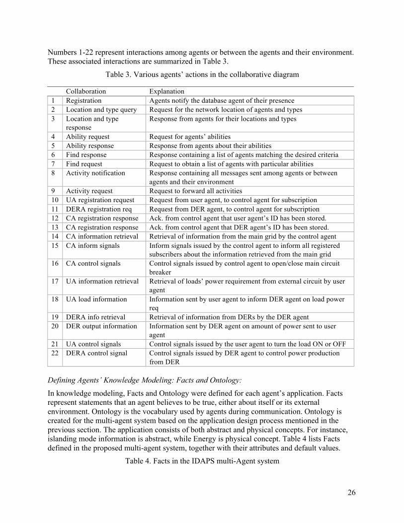
Numbers 1-22 represent interactions among agents or between the agents and their environment. These associated interactions are summarized in Table 3.

Table 3. Various agents’ actions in the collaborative diagram

Collaboration Explanation 1 Registration Agents notify the database agent of their presence 2 Location and type query Request for the network location of agents and types 3 Location and type

response Response from agents for their locations and types

4 Ability request Request for agents’ abilities 5 Ability response Response from agents about their abilities 6 Find response Response containing a list of agents matching the desired criteria 7 Find request Request to obtain a list of agents with particular abilities 8 Activity notification Response containing all messages sent among agents or between

agents and their environment 9 Activity request Request to forward all activities 10 UA registration request Request from user agent, to control agent for subscription 11 DERA registration req Request from DER agent, to control agent for subscription 12 CA registration response Ack. from control agent that user agent’s ID has been stored. 13 CA registration response Ack. from control agent that DER agent’s ID has been stored. 14 CA information retrieval Retrieval of information from the main grid by the control agent 15 CA inform signals Inform signals issued by the control agent to inform all registered

subscribers about the information retrieved from the main grid 16 CA control signals Control signals issued by control agent to open/close main circuit

breaker 17 UA information retrieval Retrieval of loads’ power requirement from external circuit by user

agent 18 UA load information Information sent by user agent to inform DER agent on load power

req 19 DERA info retrieval Retrieval of information from DERs by the DER agent 20 DER output information Information sent by DER agent on amount of power sent to user

agent 21 UA control signals Control signals issued by the user agent to turn the load ON or OFF 22 DERA control signal Control signals issued by DER agent to control power production

from DER Defining Agents’ Knowledge Modeling: Facts and Ontology:

In knowledge modeling, Facts and Ontology were defined for each agent’s application. Facts represent statements that an agent believes to be true, either about itself or its external environment. Ontology is the vocabulary used by agents during communication. Ontology is created for the multi-agent system based on the application design process mentioned in the previous section. The application consists of both abstract and physical concepts. For instance, islanding mode information is abstract, while Energy is physical concept. Table 4 lists Facts defined in the proposed multi-agent system, together with their attributes and default values.

Table 4. Facts in the IDAPS multi-Agent system

27

Facts Additional Attributes Default Value islandmode is_island: Boolean

main_cb_status: Boolean id: String outageDuration: String outageHour: String

is_island: false main_cb_status:true id: n/a outageDuration: n/a outageHour: n/a

criticalCB c1cb_status: Boolean c1cb_status: true noncriticalCB nc1cb_status: Boolean nc1cb_status: true DERspecs sendDERinfo: Boolean

DER_Cost: String UserAgentNameSpecs: String

sendDERinfo: false DER_Cost: “0” userAgentNameSpecs: n/a

ua_DERcmd der_required_power: String send_der_cmd: Boolean UserAgentName: String

der_require_power: 0.0 send_der_cmd: false userAgentName: n/a

re_uaDERcmd required_power: String UserAgentName: String

require_power: 0.0 userAgentName: n/a

dg_DERcmd der_produced_pwr: String send_der_cmd: Boolean userAgents: String

der_produced_pwr: 0.0 send_der_cmd: false userAgents: n/a

re_dgDERcmd produced_pwr: String sendDERCntrlCmd: String

produced_pwr: 0.0 sendDERCntrlCmd: false

agentsName name: String name: n/a agentRegistered name: String name: n/a inIDAPS name: String

isInIDAPS: Boolean name: n/a isInIDAPS: false

More detailed information on this topic can be found in [75, 76].

D) Agent Decision Criteria During Normal Operation:

During normal operations, the overall objective of multi-agent collaboration was designed to achieve look-ahead heterogeneous dispatch by controlling both loads and generator. The loads and generators were controlled separately.

• Generator control: DERs were dispatched according to their merit order in responding to the fluctuation in the demand for electricity. The entire amount of energy generated from renewable energy sources such as solar cells or wind turbines were injected into the distribution circuit. Mixed-integer linear programming was used to solve this scheduling problem. The decision variables, the objective function and the constraints are described below. Decision variables:

DER output (Xi,j) to be dispatch at each hour of the day

Objective function: Minimize the operating cost at each hour of the day.

28

Minimize

€

ai ⋅ Xi( )i=1

n

∑

where Xi : Decision variables, power set point (kW) of DER i aj: Operating cost ($/kWh) of DER i

Constraints:

1. All loads must be served on demand, except for the deferrable ones.

For each hour,

€

Xi( ) ≥ Li=1

n

∑ L is load requirement (kW)

2. The cumulative fuel used must still be less than the available fuel as indicated by fuel sensors.

For each hour,

€

0 ≤ Xi ≤ Ci ⋅ Fi

Where: Ci: Capacity of DER i (kW) Fi: Fuel availability indicator of DER i, if fuel is available Fi = 1, otherwise Fi = 0

3. The cumulative emission produced must still be less than the allowable emission limit.

For each hour,

€

0 ≤ Xi ≤ Ci ⋅ Ei

Where: Ci: Capacity of DER i (kW) Ei: Emission limit indicator, if the total emission is still within the available

range Ei = 1, otherwise Ei = 0

• Load control: during the grid-connected mode, the load control strategy was set to be responsive to the real-time electricity price during a non-emergency condition. Load control strategies were discussed in Section 4.2.

During Outage Conditions: During upstream outage conditions, the IDAPS microgrid was designed to disconnect itself from the utility grid and secure critical loads according to the given prioritized list. Some non-critical loads could also be secured depending upon the user’s preference. During each simulation, the first step was to identify critical loads and their priority. That is, each homeowner was asked to identify their critical loads to be secured during an event of an upstream outage. Priority of these critical loads was also identified. If available generation was not sufficient to secure all critical loads, the least important critical loads were shed. In the simulation, a homeowner could also specify the time of day when he/she would like to operate their non-critical loads during emergencies. As long as there was excess capacity from emergency generators, and expenses required to run these loads were within a reasonable range, selected non-critical loads would be secured during the chosen duration.

29

4.4 Task 4: Development IP-based Communication Interfaces for Connecting between the IDAPS Physical-Cyber Components

A) Task Description The objective of this task was to demonstrate how a connection between the IDAPS hardware elements and the IDAPS multi-agent decision support systems could be established using TCP/IP Client/Server socket communications.

B) TCP/IP Connection In the simulated environment, the multi-agent system connected to the microgrid in the MATLAB/Simulink environment over a TCP/IP connection. This allowed the microgrid to be controlled remotely by the multi-agent system from any location. A third party TCP server implementable in MATLAB Simulink was used to establish the TCP connectivity. Socket programming was carried out in agents’ external java classes. The third party TCP server was capable of managing 62 outputs and unlimited number of inputs. The server allowed only a single TCP connection at a time and followed a specific format for the input/output messages. This limited our control over the connection between the multi-agent system and the microgrid because each agent (a user agent, a DER agent and a control) required a separate TCP connection to the microgrid. To handle the situation a middle server was developed.

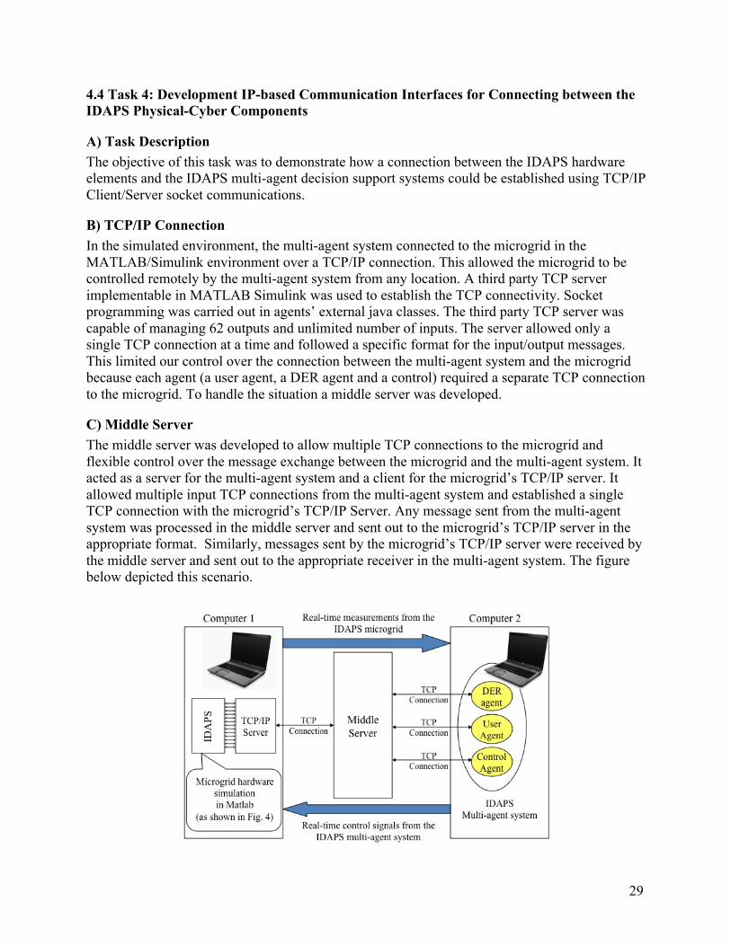
C) Middle Server The middle server was developed to allow multiple TCP connections to the microgrid and flexible control over the message exchange between the microgrid and the multi-agent system. It acted as a server for the multi-agent system and a client for the microgrid’s TCP/IP server. It allowed multiple input TCP connections from the multi-agent system and established a single TCP connection with the microgrid’s TCP/IP Server. Any message sent from the multi-agent system was processed in the middle server and sent out to the microgrid’s TCP/IP server in the appropriate format. Similarly, messages sent by the microgrid’s TCP/IP server were received by the middle server and sent out to the appropriate receiver in the multi-agent system. The figure below depicted this scenario.

30

Fig. 15. Middle server implementation

4.5 Task 5: Simulation and Evaluation of the Microgrid in both Parallel and Islanded Operations

A) Task Description In order to test this idea, we simulated and analyzed the proposed IDAPS microgrid concept using realistic data from Virginia Tech Electric Service (VTES). The Virginia Tech local distribution network was an ideal example of an interconnected microgrid in a small university town.

B) Assumptions The following assumptions were made during the simulation:

• The electric power infrastructure was available to support load and generator control. • The communication infrastructure was available to support the communications among

various physical devices in the microgrid. • Sufficient DER capacity was available to secure critical loads. • The IP-addressable interface was available to support connections among all IDAPS

physical devices and the agents.

C) Scenario Description A section of a distribution circuit from VTES was used as a basis for this simulation study. The IDAPS microgrid was simulated in the following scenarios to demonstrate its ability to operate in parallel and islanded operations. Scenario 1: Demand management during normal operation

The objective of this scenario was to showcase, during the non-emergency operation, that the IDAPS energy management system could perform load control and the level of load control depended on hourly electricity prices and load types. The results shown in Section 5 -- the results and discussion section -- illustrated that the IDAPS demand management features would reduce the peak demand, resulting in the reduction in demand charges from a local electric utility. Scenario 2: Islanding and securing critical loads during an emergency

The objective of this scenario was to illustrate the ability of multiple IDAPS agents working in collaboration to operate the microgrid in the islanded operation. The IDAPS microgrid was simulated for 24 hours, assuming that the outage occurred at 5:00PM for three hours. The simulation also focused on how the IDAPS agents detected the upstream fault, as well as how voltage and frequency changed during islanding and re-synchronizing of the microgrid after the upstream fault was cleared.

Scenario 3: Serving non-critical loads during an emergency The objective of this scenario was to showcase that the excess capacity from the DER unit after serving critical loads could be shared among non-critical loads in the community. As a result, a DER unit can be fully utilized in any given emergency event.

31

5. Results & Discussions All tasks were completed as planned. The project accomplishments were summarized below.

Tasks Tasks accomplished

1. Development of IDAPS device models

Developed/modified simulation models for PV generators, wind turbines, microturbines, fuel cell and battery storage in Matlab for used in the simulation; Developed load models.

2. Development of local control algorithms to control IDAPS device models

Developed local control for DER devices and load control strategies.

3. Development of an IDAPS energy management system

Defined the agent environment, the agent architecture, and the agent decision criteria

4. Development of IP-based communication interface

Established a TCP/IP connection between the IDAPS hardware elements and the IDAPS decision support system in a simulated environment

5. Simulation and evaluation of the microgrid in both parallel and islanded operations

Simulated the IDAPS microgrid in parallel operation; Simulated the IDAPS microgrid in islanded operation; Evaluated the results and submitted the final report

32

5.1 Task 1: Development of IDAPS Device Models

A) PV Generators – Sample Model Outputs The model of a PV generator was developed in Matlab/Simulink. Fig. 16 illustrates the model mask captured from Matlab, together with the description of the model’s inputs/outputs.

As shown in Fig. 16, inputs required include:

-­‐ Open-circuit voltage (Voc), -­‐ Number of cells connected in series (Ns), -­‐ Short-circuit current (Isc), -­‐ Number of cells connected in parallel (Np), -­‐ Maximum module power (Pmax), -­‐ Temperature coefficient of open-circuit

voltage, and -­‐ Temperature coefficient of short-circuit

current.

These parameters can be easily obtained from a manufacturer’s datasheet. Additional inputs to the model are cell temperature and solar irradiation, which can be obtained from historical data.

Fig. 16. PV model

The model outputs were validated by comparing the I-V curve outputs with the I-V curves given by the manufacturer. As shown below, the I-V curves generated by the developed model were very similar to those of the manufacturer, using the parameters of a BP-4175 175W PV module.

Fig. 17. The I-V curve from the manufacturer for BP-4175 175W PV module (left); the I-V curve generated by the developed model (right)

33

B) Wind Turbines – Sample Model Outputs As discussed in Section 4.1, a wind turbine generator was modeled as a wind turbine section connected with an electrical generator section. Fig. 18 illustrates the model mask captured from Matlab. Model inputs were (1) the generator speed in per unit of the nominal speed of the generator, and (2) the wind speed in m/s. The output of the wind turbine model was the three-phase power that could be directly connected to the electrical grid.

Fig. 18. Wind turbine model = wind turbine + asynchronous generator

The outputs of the developed wind turbine model are presented in Fig. 19. Fig. 19 (top) displays the active power (yellow) and reactive power (pink) outputs of the developed wind turbine model in kW and kVAR, respectively, when the wind speed decreases from 15 m/s to 10 m/s in the middle of the simulation. The power output decreases as the wind speed decreases. The wind turbine absorbs reactive power while producing electrical power output. Fig. 19 (bottom) displays the three-phase electrical output -- voltage (yellow) and current (pink) -- in per unit.

Pow

er (k

W)

Rea

ctiv

e Po

wer

(k

VA

R)

Vol

tage

, Cur

rent

(P

er U

nit)

Fig. 19. Electrical outputs of wind turbine:

Top: Power (yellow) and Reactive Power (pink); Bottom: Voltage (yellow) and Current (pink)

34

C) Microturbines – Sample Model Outputs As discussed in Section 4.1, two microturbine models were developed: the detailed and the simplified models. Fig. 20 illustrates the sample outputs of the detailed microturbine model, e.g. the line-to-line voltage of a 30kW microturbine at 480V line-to-line.

Line-to-line voltage (Volt) during the hot start

when simulating from 0 to 50 seconds Snap shot of the line-to-line voltage (Volt)

around t = 50 second

Fig. 20. Sample outputs of the detailed microturbine model x-axis is the simulation time in second; y-axis is the voltage magnitude;

Fig. 21 illustrates the sample outputs of the simplified microturbine model, e.g. the power output of a 30kW microturbine during the hot start (left) and the cold start (right).

Fig. 21. Sample outputs of the simplified microturbine model

Characteristics during the hot start (left); Characteristics during the cold start (right)

D) Fuel Cells and Battery Storage Model Since the fuel cell and the battery storage models available in Matlab/Simulink were used in the simulation, the model outputs could be found in Matlab 2009 reference guide. Therefore, the sample results of these two models are not discussed here.

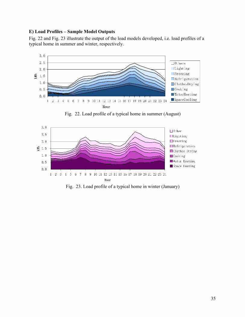
35

E) Load Profiles – Sample Model Outputs Fig. 22 and Fig. 23 illustrate the output of the load models developed, i.e. load profiles of a typical home in summer and winter, respectively.

Fig. 22. Load profile of a typical home in summer (August)

Fig. 23. Load profile of a typical home in winter (January)

36

5.2 Task 2: Development of Local Control Algorithms to Control IDAPS Device Models

A. Grid Connected Mode - Sample Results As shown in Fig. 24, the test circuit comprises one distributed generator, a grid interface section – an inverter, a PWM controller and an RLC filter, loads and measurements, as well as an isolation transformer and the grid.

Fig. 24. Test circuit for the grid connected operation

The circuit as shown was simulated for 0.2 seconds to illustrate the impact of the decrease in DER output on the voltage signal at the interconnection point. Fig. 25 displays the simulation results when the power output from a DER unit decreases from 50 kW to 25 kW at t = 0.1 seconds.

Distributed generator

Grid interface: Inverter, PWM controller, filter

Loads & measurements

Isolation transformer & the grid

Bus B1 Bus B2

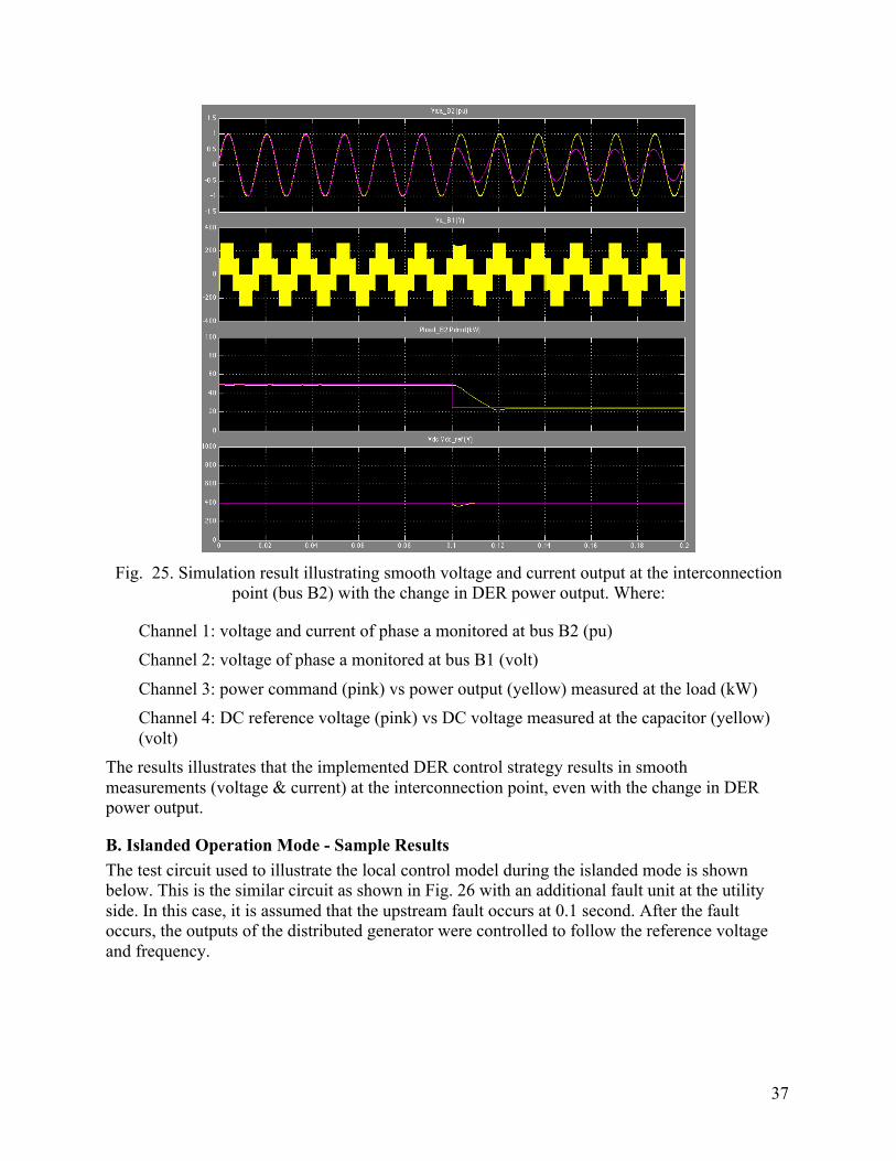
37

Fig. 25. Simulation result illustrating smooth voltage and current output at the interconnection

point (bus B2) with the change in DER power output. Where:

Channel 1: voltage and current of phase a monitored at bus B2 (pu) Channel 2: voltage of phase a monitored at bus B1 (volt)

Channel 3: power command (pink) vs power output (yellow) measured at the load (kW) Channel 4: DC reference voltage (pink) vs DC voltage measured at the capacitor (yellow) (volt)

The results illustrates that the implemented DER control strategy results in smooth measurements (voltage & current) at the interconnection point, even with the change in DER power output.

B. Islanded Operation Mode - Sample Results The test circuit used to illustrate the local control model during the islanded mode is shown below. This is the similar circuit as shown in Fig. 26 with an additional fault unit at the utility side. In this case, it is assumed that the upstream fault occurs at 0.1 second. After the fault occurs, the outputs of the distributed generator were controlled to follow the reference voltage and frequency.

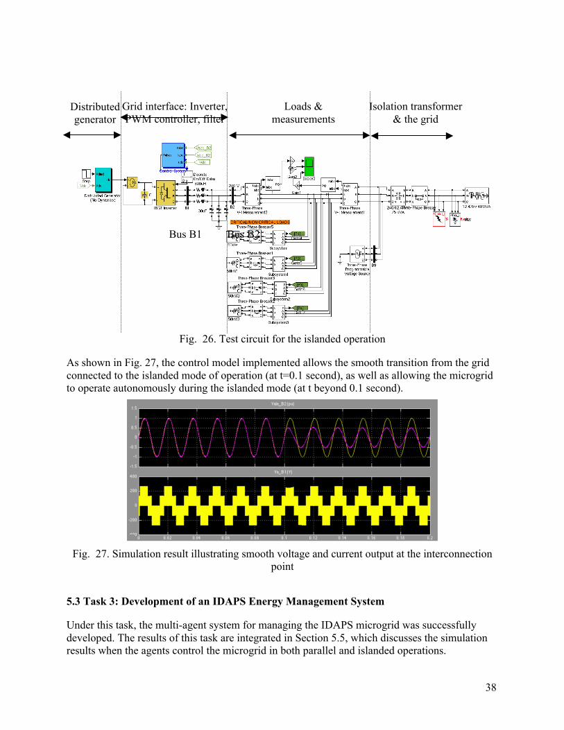
38

Fig. 26. Test circuit for the islanded operation

As shown in Fig. 27, the control model implemented allows the smooth transition from the grid connected to the islanded mode of operation (at t=0.1 second), as well as allowing the microgrid to operate autonomously during the islanded mode (at t beyond 0.1 second).

Fig. 27. Simulation result illustrating smooth voltage and current output at the interconnection

point

5.3 Task 3: Development of an IDAPS Energy Management System

Under this task, the multi-agent system for managing the IDAPS microgrid was successfully developed. The results of this task are integrated in Section 5.5, which discusses the simulation results when the agents control the microgrid in both parallel and islanded operations.

Distributed generator

Grid interface: Inverter, PWM controller, filter

Loads & measurements

Isolation transformer & the grid

Bus B1 Bus B2

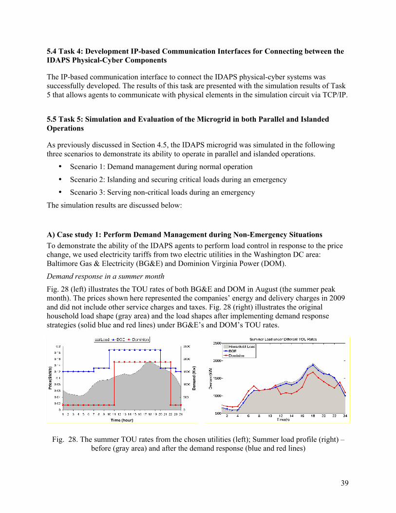
39

5.4 Task 4: Development IP-based Communication Interfaces for Connecting between the IDAPS Physical-Cyber Components

The IP-based communication interface to connect the IDAPS physical-cyber systems was successfully developed. The results of this task are presented with the simulation results of Task 5 that allows agents to communicate with physical elements in the simulation circuit via TCP/IP.

5.5 Task 5: Simulation and Evaluation of the Microgrid in both Parallel and Islanded Operations

As previously discussed in Section 4.5, the IDAPS microgrid was simulated in the following three scenarios to demonstrate its ability to operate in parallel and islanded operations.

• Scenario 1: Demand management during normal operation

• Scenario 2: Islanding and securing critical loads during an emergency • Scenario 3: Serving non-critical loads during an emergency

The simulation results are discussed below:

A) Case study 1: Perform Demand Management during Non-Emergency Situations To demonstrate the ability of the IDAPS agents to perform load control in response to the price change, we used electricity tariffs from two electric utilities in the Washington DC area: Baltimore Gas & Electricity (BG&E) and Dominion Virginia Power (DOM). Demand response in a summer month

Fig. 28 (left) illustrates the TOU rates of both BG&E and DOM in August (the summer peak month). The prices shown here represented the companies’ energy and delivery charges in 2009 and did not include other service charges and taxes. Fig. 28 (right) illustrates the original household load shape (gray area) and the load shapes after implementing demand response strategies (solid blue and red lines) under BG&E’s and DOM’s TOU rates.

Fig. 28. The summer TOU rates from the chosen utilities (left); Summer load profile (right) – before (gray area) and after the demand response (blue and red lines)

40

As shown, the demand response strategies implemented by IDAPS agents helped lower the system peak demand, under both BG&E and DOM rate structures. This resulted in the reduction in a portion of the demand charge ($/kW) imposed by a utility. With the IDAPS demand management strategy, lower system peaks were expected under the pricing scheme with higher variation in peak and off-peak rates. In this case, the level of demand response would be higher under DOM’s TOU rates, as compared to that under BG&E’s TOU rates.

Demand response in a winter month Fig. 29 (left) illustrates the TOU rates of both BG&E and DOM in January (the winter peak month). The prices shown here represented the companies’ energy and delivery charges in 2009 and did not include other service charges and taxes. Fig. 29 (right) illustrates the original household load shape (gray area) and the load shapes after implementing demand response strategies (solid lines) under BG&E’s and DOM’s TOU rates.

Fig. 29. The summer TOU rates from the chosen utilities (left); Summer load profiles (right) – before (gray area) and after the demand response (blue and red lines)

Similar to the results in the summer month, the demand response strategies implemented by IDAPS agents could help lower the system peak demand, under both BG&E and DOM rate structures in the winter month as well. More detailed description of IDAPS control algorithms during non-emergencies can be found in [77, 78].

B) Case study 2: Island the Microgrid once a Fault is Detected and Secure Critical Loads during an Emergency This scenario illustrated the ability of multiple agents to work in collaboration to operate the microgrid in the islanded mode. The IDAPS microgrid was simulated for 24 hours, assuming that the outage occurred at 5:00PM for three hours. The simulation also focused on how IDAPS agents detected the upstream fault, voltage and frequency deviation during islanding and re-synchronizing of the microgrid after the upstream fault was cleared. Fig. 30 illustrates the load profiles of one house in this microgrid. The result clearly shows that as soon as an outage was detected the multi-agent system performed its actions to secure critical loads prioritized according to the homeowner’s choice. In this case, the critical loads were secured and non-critical loads were disconnected.

41

Fig. 30. Load profile with agents securing critical loads during the outage between 5-8pm. All

non-critical loads are shed.

The upstream fault was applied to the circuit at 5 PM. As soon as upstream fault was detected, the IDAPS agents islanded the microgrid. The result shown in Fig. 31 is a snapshot of the event at around 5 PM. This illustrates the fluctuation in voltage and current at the interconnection point of the IDAPS microgrid and the utility system, from 0.1 seconds before the fault and 0.2 seconds after the fault. This helps determine how quickly the multi-agent system can perform its actions to isolate the microgrid while maintaining the system stability.

Fig. 31. The variation of 60Hz voltage and current waveforms measured at the interconnection

point before and after the upstream outage applied to the circuit.

A. During the Grid-Connected Mode (before 5PM) The microgrid’s voltage and frequency were controlled such that they followed the grid’s voltage and frequency, roughly at 1 per unit and 60 Hz, respectively. As shown, the voltage (yellow) was always kept at around 1 per unit. The current (pink) indicated the current produced by the DER. Before the upstream fault occurred, the DER unit supplied some power to the microgrid at about 50% of its rated power.

B. During the Transition (at 5PM) Once the control agent detected the fault at 5PM, the control agent informed the user agent and the DER agent, both of which exchanged information and determined the amount of loads to be shed and the amount of power to be produced internally in order to stabilize the microgrid. The

42

control agent sent a control signal to isolate the microgrid by disconnecting the main circuit breaker as soon as the upstream outage was detected. Depending on the pre-defined load priority set by a user and the available internal generation, the user agent disconnected non-critical loads and certain critical loads. In this case, we assumed that the DER could fully support connected critical loads without any energy limitation during the outage. In other words, the DER could increase its output instantaneously with the help of battery storage once the microgrid islanded. Thus, the user agent only disconnected the non-critical loads and left the critical loads intact. All agent actions – from detecting the fault, disconnecting the main circuit breaker, disconnecting the non-critical loads to stabilizing the grid – were accomplished within about half an electrical cycle, i.e. less than 0.008 second for a 60-Hz system. The DER fault current as shown was limited by the inverter rating in the case of an inverter-based DER. C. During the Islanded Mode (5PM-8PM):

After the fault occurred at 5PM, the IDAPS microgrid was disconnected from the main grid. When the microgrid operated in the island mode, the grid interface unit tried to control the DER output voltage at 1 per unit and the frequency at 60Hz. The user agent and the DER agent balanced the demand and supply within the microgrid. The total system load was reduced to its critical loads and the DER produced almost at its full capacity internally to supply these critical loads. This can be seen in Fig. 31 after 5PM that the current output from DER increased to almost 1 per unit. D. During Resynchronization to the Main Grid (at 8PM)

At 8:00PM, the upstream fault was cleared. Fig. 32 illustrates the system parameters at 8PM.

Fig. 32. Simulation results during the synchronization of the microgrid to the main grid.

43

The first graph in Fig. 32 illustrates the fluctuation in voltage and current at the microgrid interconnection point in per unit from 0.1 seconds before the fault was cleared and 0.2 seconds after the fault was cleared. Fig. 32 also displays the DER output power in kW in the second graph; and in the third graph, the voltage difference between the RMS voltage at the microgrid side and the RMS voltage at the main grid side in volts. During the upstream outage, the main grid voltage was collapsed, while the microgrid maintained its voltage at 1 per unit. Therefore, the voltage difference between the main grid and the microgrid, as shown in Fig. 32, was 240V during the islanded mode. As the upstream circuit was restored at 8PM, the main grid voltage gradually increased. Therefore, the voltage difference, as shown in Fig. 32, gradually decreased at around 8PM.

The control agent monitored this voltage difference, as well as the frequency of both systems. Once it detected that the voltage and frequency differences remained below a certain threshold, the control agent issued three control signals. These control signals were to (i) close the main switch; (ii) reconnect non-critical load circuit breakers; and (iii) decrease the DER output to prevent instantaneous overshoot in the system’s voltage and current. In this case, at 0.02 seconds after 8PM, the control agent issued the synchronization signal. The system voltage was again stabilized at 1 per unit. There was minor current overshooting in the first half a cycle. Then again the system was stabilized. The DER output demonstrated a small ripple for about 0.1 seconds before arriving at its steady state.

C) Case study 3: Secure Selected Non-Critical Loads during Emergencies In this scenario, it was assumed that the outage started from 12:20AM until midnight the next day. Since there was excess capacity from the DER unit after serving critical loads, this excess capacity would be shared by some of the non-critical loads in the community. Here, we presented results of the IDAPS agent management system that allowed the limited DER capacity to be shared among non-critical loads during outages. Before the outage occurred or during the outage, homeowners or facility owners were asked to enter the maximum amount of money that ones would like to spend on non-critical loads. Users also were asked to select the time of the day that they would like to operate non-critical loads. This case study demonstrated how non-critical loads were secured within the IDAPS microgrid, during an outage that lasted almost 24 hours. In this case, we focused on a community of five houses. Table 5 showed the $ limit and hours for non-critical load operation selected by the owners of five houses.

Table 5. Requirements to serve non-critical loads during outages

House 1 House 2 House 3 House 4 House 5

$ Limit $10 $15 $20 $25 $35

Selected non-critical load operating hours

01:00-02:00 05:00-10:00 17:00-22:00

01:00-02:00 07:00-11:00 19:00-22:00

05:00-09:00 17:00-21:00

07:00-10:00 19:00-22:00

05:00-11:00 17:00-23:00

44

As a standard practice, once the agents detected an upstream outage at 12:20AM, all critical loads were secured. The decision to select which non-critical loads to be served depended on the load priority (for example, non-critical loads in critical facility like hospital are of higher priority), amount of money homeowners were willing to pay for their non-critical loads to be served, and their desired duration of operation. Fig. 33 illustrates additional DER output to serve non-critical loads when needed.

Fig. 33. DER output (kW) to serve critical and non-critical loads

Fig. 34-38 illustrates the results of non-critical load operation for houses no. 1-5, respectively.

Fig. 34. Non-critical load operation (house 1)

In this case, the homeowners selected to operate non-critical loads during the following hours: (a) 01:00-02:00 (b) 05:00-10:00 (c) 17:00-22:00

Limitation $10.

45

Fig. 35. Non-critical load operation (house 2)

In this case, the homeowners selected to operate non-critical loads during the following hours: (a) 01:00-02:00 (b) 07:00-11:00 (c) 19:00-22:00

Limitation $15.

Fig. 36. Non-critical load operation (house 3)

In this case, the homeowners selected to operate non-critical loads during the following hours: (a) 05:00-09:00 (b) 17:00-21:00

Limitation $20.

Fig. 37. Non-critical load operation (house 4)

In this case, the homeowners selected to operate non-critical loads during the following hours: (a) 07:00-10:00 (b) 19:00-22:00

Limitation $25.

46

Fig. 38. Non-critical load operation (house 5)

In this case, the homeowners selected to operate non-critical loads during the following hours: (a) 05:00-11:00 (b) 17:00-23:00

Limitation $35.

The results illustrate that the IDAPS energy management system was capable of controlling DER and loads such that critical loads could be secured during emergency and some of the non-critical loads could be served when needed.

47

6. Conclusions and Implications for Future Research In response to the DoD’s statement of need, this work was the proof-of-concept effort to study the microgrid operation in both islanded and grid-connected modes. This effort resulted in the intelligent distributed autonomous power grid that could facilitate the use of renewable energy technologies, thereby minimizing reliance on external energy resources and reducing fossil fuel consumption.

The following five tasks as proposed were accomplished: Task 1: Development of IDAPS device models

In this task, models of IDAPS physical components were developed in Matlab/Simulink. These models included solar photovoltaic modules, wind turbine generators, microturbines, fuel cells and battery storage. Task 2: Development of local control algorithms to control IDAPS device models

Local control algorithms were developed to control DER units for their grid interface. The results indicated that the control unit could accommodate the integration of DER units into the utility grid. Voltage and frequency could be controlled to follow those of the grid or follow system reference. Task 3: Development of an IDAPS energy management system

The IDAPS energy management system was developed based on agent technologies. The IDAPS energy management system comprised four agents, including DER agent, user agent, control agent and database agent. Each agent had its objectives and responsibilities. Task 4: Development of addressable IP-based communication interfaces for connecting IDAPS device models and IDAPS energy management system Under task 4, the connection between the IDAPS physical and cyber systems was successfully established. The simulation conducted under task 5 integrated this feature that allowed agents to communicate with physical elements in the simulation circuit via TCP/IP.

Task 5: Simulation and evaluation of the microgrid in both parallel and islanded operations Several scenarios were simulated to evaluate the IDAPS microgrid and its energy management system to perform demand management during the grid connected mode, and secure critical loads when an upstream fault was detected.

The simulation results demonstrated that the proposed IDAPS microgrid allowed various DER sources, including renewables, to network and collaborate in an efficient manner. This work met the proposed objective by illustrating that the IDAPS microgrid could: (i) perform demand management during normal operating condition; (ii) island the microgrid from the main grid once an upstream fault is detected; (iii) secure critical loads and shed non-critical loads according to the given priority list during emergencies; and (iv) resynchronize the microgrid to the main grid after an upstream fault is cleared. Several technical challenges were addressed by this work, including analyzing dynamic response of agent-based control strategies, defining multi-agent system’s role and definition, and evaluating on- and off-grid operation of a microgrid with

48

renewable distributed generation systems. Addressing these challenges would contribute to facilitating the implementation of renewable energy sources in a microgrid, thus enhancing energy security and reliability for the mission-critical parts of military bases and campus-type facilities.

It is possible to extend the modeling and simulation development based on this work so that it can be used to explore the feasibility of the development of microgrids in a campus-type facility. The developed simulation platform with some modifications can be used to realistically simulate and validate any proposed microgrid generation and load control algorithms. Therefore, it can be used to quantify the risks and the impact of implementing the proposed control algorithms before the actual field implementation. Based on this work, several microgrid deployment scenarios can be validated and guidelines for microgrid development can be provided.

49

Appendix A - Publications

This work has resulted in one Master’s thesis on multi-agent systems, and five publications in several IEEE conferences with full paper reviews.

• Feroze, H., “Multi-Agent Systems in Microgrids: Design & Implementation”, Master Thesis, Virginia Tech, August 2009.

• Pipattanasomporn, M., Feroze, F., and Rahman, S., “Multi-­‐agent systems in a distributed smart grid: design and implementation”, In Proc. IEEE Power System Conference & Exposition, March 18, 2009, Seattle, WA.

• Waseem, I., Pipattanasomporn, M., and Rahman, S., “Reliability benefits of distributed generation as a backup source”, In Proc. 2009 IEEE Power & Energy Society General Meeting, July 2009, Calgary, Canada.

• Shao, S., Pipattanasomporn, M., and Rahman, S., “Challenges of PHEV penetration to the residential distribution network”, In Proc. 2009 IEEE Power & Energy Society General Meeting, July 2009, Calgary, Canada.

• Zhang, T., Shao, S., Pipattanasomporn, M., and Rahman, S., “Impact of variable electricity rates on distribution feeder load shapes in a smart grid”, In Proc. IEEE PES/IAS Conference on Sustainable Alternative Energy, September 2009, Spain.

• Shao, S., Zhang, T., Pipattanasomporn, M., and Rahman, S., “Impact of TOU rates on distribution load shapes in a smart grid with PHEV penetration”, Accepted for presentation in IEEE PES Transmission & Distribution Conference & Exposition, April 2010, New Orleans, Louisiana.

50

References [1] Agrawal, P., “Overview of DOE microgrid activities”, Symposium on Microgrid, Montreal, June 23, 2006

[Online]. Available: http://der.lbl.gov/2006microgrids_files/USA/Presentation_7_Part1_Poonum-agrawal.pdf. Retrived: May 2009.

[2] EPRI. Electricity technology roadmap: 2003 summary and synthesis. Nov. 2003. Retrieved Sept 2008, from www.hoffmanmarcom.com/docs/pd&m_roadmap_2003.pdf.

[3] Sanchez, M.. Overview of microgrid research and development activities in the EU. In Proc. the 2006 Symposium on Microgrids. Montreal, Canada. Jun 23, 2006.

[4] NEDO. Project: Demonstrative Project of Regional Power Grids with Various New Energies. New Energy and Industrial Technology Development Organization (NEDO). Retrieved Sept 2008, from www.nedo.go.jp/english/activities/2_sinenergy/3/p03038e.html.

[5] CERTS Microgrid Test Bed Demonstration with American Electric Power [Online]. Available: http://certs.lbl.gov. Retrived: May 2009.

[6] Akhil, A. “Development of an energy surety microgrid for military applications”, presented at Army Installation Energy Security & Independence Conference, December 13, 2006 [Online]. Available: http://www.cecer.army.mil/techreports/ERDC-CERL_TR-07-9/Session%20II/Akhil.pdf. Retrieved: May 2009.

[7] Eto, J.H., R. Lasseter, B. Schenkman, J. Stevens, H. Volkommer, D. Klapp, E. Linton, H. Hurtado, J. Roy and N. Lewis, “CERTS microgrid laboratory test bed”, California Energy Commission, Public Interest Energy Research Program. ECE-500-2008-XXX [Online]. Available: http://certs.lbl.gov/pdf/certs-mgtb-report.pdf. Retrived: May 2009.

[8] Tatro, M. L., Covan, J. M., Robinett, R. III, Kuswa, G. W., Menicucci, D., and Jones, S. A. “Toward an energy surety future”, SANDIA report SAND2005-6281 [Online]. Available: http://www.prod.sandia.gov/cgi-bin/techlib/access-control.pl/2005/056281.pdf. Retrived: May 2009.

[9] Lorenzo, E., “Solar electricity engineering of photovoltaic systems”, Spain, ISBN: 8486505550.

[10] Hansen, A. Lars, P., Hansen, H. and Bindner H., “Models for a Stand-Alone PV System”. Risø National Laboratory, Roskilde, December 2000, ISBN 87-550-2776-8. [Online]. Available: http://www.risoe.dk/rispubl/VEA/ris-r-1219.htm.

[11] Mellit, A., Benghanem, M. and Kalogirou, S. A., “Modeling and simulation of a stand-alone photovoltaic system using an adaptive artificial neural network: proposition for a new sizing procedure”, Renewable Energy, Vol. 32, Iss. 2, February 2007.

[12] Park, M., Lee, D. and Yu, I., “PSCAD/EMTDC modeling and simulation of solar-powered hydrogen production system”, Renewable Energy, Vol. 31, Iss. 14, November 2006.

[13] Radziemska, E., “The effect of temperature on the power drop in crystalline silicon solar cells”, Renewable Energy, Vol. 28, Iss. 1, January 2003.

[14] Ross, J. N., Markvart, T. and He, W., “Modeling battery charge regulation for a stand-­‐alone photovoltaic system”, Solar Energy,Vol. 69, Iss. 3, 2000.

[15] Phang, J.C.H., Chan., D.S.H. and Phillips, J.R., “Accurate analytical method for the extraction of solar cell model parameters”, Electron. Lett. 20 10, 1984, pp. 406–408.

[16] Chan., D.S.H. and Phillips, J.R.and Phang, J.C.H., “A comparative study of extraction methods for solar cell model parameters”, Solid-St. Electron. 29 3, 1986, pp. 329–337.

[17] de blas, Torres, J.L., Prieto, E. and Garcia, A., “Selecting a suitable model for characterizing photovoltaic devices”, Renewable Energy, Vol 25, Iss. 3, March 2002.

51

[18] Petru, T. and Thiringer, T., “Modeling of wind turbines for power system studies,” Power Systems, IEEE

Transactions on , vol.17, no.4, pp. 1132-1139, Nov 2002.

[19] Malinga, B., Sneckenberger, J.E., Feliachi, A., “Modeling and control of a wind turbine as a distributed resource,” System Theory, 2003. Proceedings of the 35th Southeastern Symposium on , vol., no., pp. 108-112, 16-18 March 2003.

[20] Yazhou Lei, Mullane, A., Lightbody, G. and Yacamini, R., “Modeling of the wind turbine with a doubly fed induction generator for grid integration studies,” Energy Conversion, IEEE Transaction on , vol.21, no.1, pp. 257-264, March 2006.

[21] Yin, M., Li, G., Zhou, M. and Zhao, C., “Modeling of the Wind Turbine with a Permanent Magnet Synchronous Generator for Integration,” Power Engineering Society General Meeting, 2007. IEEE , vol., no., pp.1-6, 24-28 June 2007

[22] Rowen, W. I., “Simplified Mathematical Representations of Heavy-Duty Gas turbines”, Journal of Engineering for Power, Oct 1983, Vol. 105.

[23] Hannett, L. N. and Khan, A., “Combustion Turbine Dynamic Model Validation from Tests”, IEEE Trans. On Power Systems, Vol. 8, No. 1, Feb 1993.

[24] Al-Hinai, A. and Feliachi, A., “Dynamic model of a microturbine used as a distributed generator”, In Proceedings of the Thirty-Fourth Southeastern Symposium on System Theory, 2002, Page(s): 209 – 213.

[25] Guda, S. R., Wang, C. and Nehrir, M. H., “Modeling of Microturbine Power Generation Systems”, Electric Power Components and Systems, 34: 1027-1041, 2006.

[26] Gaonkar, D. N. and Patel, R. N., “Modeling and Simulation of Microturbine Based Distributed Generation System”, IEEE 2006.

[27] Rendon, M. A., Nascimento, M. A. R. and Mendes, P. P. C., “Load Current Control Model for a Gas Microturbine in Isolated Operation”, IEEE 2006.

[28] Correa, J.M., Farret, F.A., Canha, L.N. and Simoes, M.G., "An electrochemical-based fuel-cell model suitable for electrical engineering automation approach," Industrial Electronics, IEEE Transactions on , vol.51, no.5, pp. 1103-1112, Oct. 2004.

[29] Brooks, N., Baldwin, T., Brinson, T., Ordonez, J. and Luongo, C., "Analysis of fuel cell based power systems using EMTDC electrical power simulator," System Theory, 2004. Proceedings of the Thirty-Sixth Southeastern Symposium on , vol., no., pp. 270-274, 2004.

[30] Georgakis, D., Papathanasiou, S. and Manias, S., "Modeling and Control of a Small Scale Grid-connected PEM Fuel Cell System," Power Electronics Specialists Conference, 2005. PESC '05. IEEE 36th , vol., no., pp.1614-1620, 2005.

[31] Wang, C., Nehrir, M.H. and Shaw, S., "Dynamic models and model validation for PEM fuel cells using electrical circuits," Power Engineering Society General Meeting, 2005. IEEE , vol., no., pp. 2115 Vol. 3-, 12-16 June 2005.

[32] Matthias, D., Andrew, C., Sinclair, G. and McDonald J.R., “Dynamic model of a lead acid battery for use in a domestic fuel cell systems,” Journal of Power Sources, Vol. 161, Oct 27, 2006, pp. 1400-1411.

[33] Kuhn, E., Forgez, C., Lagonotte, P. and Friedrich, G., “Modeling Ni-MH battery using Cauer and Foster Structures, “ Journal of Power Sources, vol. 158, Aug 25, 2006, pp. 1490-1497.

[34] Ziyad M., Salameh, Casacca, M.A. and Lynch, W.A., "A Mathematical Model for Lead-Acid Batteries", IEEE Trans. on Energy Conversion. Vol. 7,No. 1, March 1992.

[35] Manwell, J.F. and McGowan, J.G., “Extension of the kinetic battery model for Wind/Hybrid Power Systems”, In proceedings of EWEC 284-289, 1994.

[36] Facinelli, W.A., “Modelling and Simulation of Lead Acid Batteries for Photovoltaic Systems”, In the proceedings of the 18th IECEC, 1983.

52

[37] Hyman, E., Spindler, W. and Fatula, J.F., “Phenomenological Discharge Voltage Model for Lead Acid

Batteries”, In the proceedings of AIChe Meeting, Mathematical Modelling of Batteries, 1986.

[38] Tremblay, O., Dessaint, L.A. and Dekkiche, A. I., “A Generic Battery Model for the Dynamic Simulation of Hybrid Electric Vehicles”, IEEE 2007.

[39] H. S. Nwana, “Software agents: an overview”, The knowledge engineering review, 11, No 3, pp. 205-244, 1996.

[40] J. M. Bradshaw, ‘Software agents’, Cambridge, MA, MIT Press, 1997.

[41] N. Jennings, and M. Wooldridge, “Software agents”, IEE Review, pp 17-20, 1996.

[42] S. Franklin, and A. Graesser, “Is it an agent, or just a program?: a taxonomy for autonomous agents”, in Proc. The 3rd International Workshop on Agent Theories, Architectures and Languages, Springer-Verlag, pp. 21-35, 1996.

[43] S. Song, S. Shin, and M. Kim, “Multiagent-based defensive strategy system for military simulation”, in Proc. 10th Agent Computing and Multi-Agent Systems: PRIMA, pp. 329-338, 2007.

[44] D. R. Klose, “Agent-based systems key enabler for the army’s future force”, in Proc. International Conference on Integration of Knowledge Intensive Multi-Agent Systems, pp. 249 - 254, 2003.

[45] T. M. Cioppa, T. W. Lucas, and S. M. Sanchez, “Military applications of agent-based simulations”, in Proc. of the 36th conference on Winter simulation, pp. 171 – 180, 2004.

[46] P. Mc Dermott, and C. O’Riordan, “A system for multi-agent information retrieval”, in Proc. of the 13th Irish International Conference on Artificial Intelligence and Cognitive Science, Springer-Verlag, pp. 70 – 77, 2002.

[47] T. Bui, and J. Lee, “An agent-based framework for building decision support systems”, in Special issue on decision support technologies for complex and open organizations, pp. 225-237, 1999.

[48] X. Xue, X. Li, Q. Shen, and Y. Wang, “An agent-based framework for supply chain coordination in construction”, in Proc. International Conference for Construction Information Technology, pp. 413-430, 2005.

[49] P. Davidsson, L. Henesey, L. Ramstedt, J. Tornquist and F. Wernsdedt, “An analysis of agent-based approaches to transport logistics”, in Agents in Traffic and Transportation Workshop No. 3, pp. 255-271, 2005.

[50] S. S. Manvi, and P. Venkataram, “Applications of agent technology in communications: a review”, in Agents in Computer Communications, pp. 1493 – 1508, 2004.

[51] K. A. Karasavvas, R. Baldock, and A. Burger, “Bioinformatics integration and agent technology”, in Journal of Biomedical Informatics, Vol. 37, Issue 3, pp. 205 – 219, 2004.

[52] C. Lucas, M. A. Zia, M. R. A. Shirazi, and A. Alishahi, “Development of a multi-agent information management system”, in Proc. of IEEE Power Tech, Vol. 3, pp. 6, 2001

[53] V. Marik, and D. McFarlane, “Industrial adoption of agent based technologies”, in IEEE Intelligent Systems, Vol. 20, Issue 1, pp. 27-35, 2005.

[54] P. Marques, P. Simoes, L. Silva, F. Boavida, and J. Silva, “Providing applications with mobile agent technology”, in Proc. of IEEE Open Architectures and Network Programming, pp. 129-136, 2001

[55] J. Oleskow, M. Fertsch, and P. Golinska, “Agent-based technology as a tool for the integration of manufacturing systems”, in World Automation Congress, pp. 1-6, 2006.

[56] J. Hossack, S.D.J. Mcanhur, J.R. Mcdonald, J. Stokoe and T. Cumming, “A multi-agent approach to power system disturbance diagnosis”, in Proc. of International conference on power system management and control, Vol. 488, pp. 317-322, 2002.

53

[57] S.D.J. McArthur, E.M. Davidson, J.A. Hossack, and R. McDonald, “Automating power system fault

diagnosis through multi-agent system technology”, in Proc. of the 37th Hawaii International Conference on System Sciences, 8pp, 2004.

[58] T. Nagata and H. Sasaki, “A multi-agent approach to power system restoration”, IEEE Transactions on Power Systems, Vol. 17, pp. 457-462, 2002

[59] H.F. Wang, “Multi-agent co-ordination for the secondary voltage control in power system contingencies”, in Proc. of IEE Generation, Transmission and Distribution, Vol. 148, pp. 61-66, 2001.

[60] H.F. Wang, “Multi-agent co-ordination for the secondary voltage control in power system contingencies”, in Proc. of IEE Generation, Transmission and Distribution, Vol. 148, pp. 61-66, 2001.

[61] S. D. J. McArthur, E. M. Davidson, V. M. Catterson, A. L. Dimeas, N. D. Hatziargyriou, F. Ponci, and T. Funabashi, “Multi-agent systems for power engineering applications—Part I: concepts, approaches, and technical challenges”, IEEE Transaction on Power Systems, Vol. 22, Issue 4, pp. 1743 – 1752, Nov. 2007.

[62] S. D. J. McArthur, E. M. Davidson, V. M. Catterson, A. L. Dimeas, N. D. Hatziargyriou, F. Ponci, and T. Funabashi, “Multi-agent systems for power engineering applications—Part II: technologies, standards, and tools for building multi-agent systems”, IEEE Transaction on Power Systems, Vol. 22, Issue 4, pp. 1753 - 1759, Nov. 2007.

[63] J. D. Kueck, R. H. Staunton, S. D. Labinov, and B. J. Kirby, Microgrid energy management system, CERTS, ORNL/TM-2002/242, Jan 2003 [Online]. Available: http://www.ornl.gov/sci/btc/apps/Restructuring/OR NLTM2002242rev.pdf.

[64] L. Phillips, M. Link, R. Smith, and L. Weiland, Agent-based control of distributed infrastructure resources. Sandia National Laboratories, SAND2005-7937, Jan 2006 [Online]. Available: www.sandia.gov/scada/ documents/sand_2005_7937.pdf.

[65] A. Dimeas and N.D Hatziargyriou, “Operation of a multiagent system for microgrid control”, IEEE transaction on Power Systems, Vol. 20, No. 3, pp. 1447-1455, 2005.

[66] A. Dimeas and N.D Hatziargyriou, “Operation of a multiagent system for microgrid control”, in Power Engineering Society General Meeting, Vol. 1, pp. 55-58, 2004.

[67] T. Nagata, Y. Tao, H. Sasaki, and H. Fujita, “A Multi-agent Approach to Distribution System Restoration”, in Power Engineering Society General Meeting, Vol. 2, page(s) 660, 2003.

[68] Heier, S., “Grid Integration of Wind Energy Conversion Systems,” John Wiley & Sons Ltd, 1998, ISBN 0-471-97143-X.

[69] Guda, S. R., Wang, C. and Nehrir, M. H., “Modeling of Microturbine Power Generation Systems”, Electric Power Components and Systems, 34: 1027-1041, 2006.

[70] Rowen, W. I., “Simplified Mathematical Representations of Heavy-Duty Gas turbines”, Journal of Engineering for Power, Oct 1983, Vol. 105.

[71] Heier, S., “Grid Integration of Wind Energy Conversion Systems,” John Wiley & Sons Ltd, 1998, ISBN 0-471-97143-X.

[72] Energy Nexus Group, “Technology Characterization: Microturbines”, Prepared for Environmental Protection Agency, Climate Protection Partnership Division, March 2002.

[73] CERTS, “Behavior of Capstone and Honeywell Microturbine Generators during Load Changes”, Consultant Report, February 2004.

[74] Reload Database

[75] Feroze, H., “Multi-Agent Systems in Microgrids: Design & Implementation”, Master Thesis, Virginia Tech, August 2009.

54

[76] Pipattanasomporn, M., Feroze, F., and Rahman, S., “Multi-­‐agent systems in a distributed smart grid: design

and implementation”, In Proc. IEEE Power System Conference & Exposition, March 18, 2009, Seattle, WA.

[77] Shao, S., Pipattanasomporn, M., and Rahman, S., “Challenges of PHEV penetration to the residential distribution network”, In Proc. 2009 IEEE Power & Energy Society General Meeting, July 2009, Calgary, Canada.

[78] Shao, S., Zhang, T., Pipattanasomporn, M., and Rahman, S., “Impact of TOU rates on distribution load shapes in a smart grid with PHEV penetration”, Accepted for presentation in IEEE PES Transmission & Distribution Conference & Exposition, April 2010, New Orleans, Louisiana.