FINAL REPORT ITMMA TML Analysis of the · PDF fileAnalysis of the Consequences of Low Sulphur...

Analysis of the Consequences of Low Sulphur Fuel Requirements

Study commissioned by

European Community Shipowners’ Associations (ECSA)

FINAL – 29 January 2010

1

Analysis of the Consequences of Low Sulphur Fuel Requirements

Report commissioned by

European Community Shipowners’ Associations (ECSA)

Report drafted by

Prof. Dr. Theo Notteboom, ITMMA – University of Antwerp and

Dr. Eef Delhaye, Kris Vanherle, Transport & Mobility Leuven

FINAL – 29 January 2010

Prof. Dr. Theo Notteboom ITMMA – UNIVERSITY OF ANTWERP KEIZERSTRAAT 64 2000 ANTWERPEN BELGIUM http://www.itmma.ua.ac.be TEL +32 (3) 265.51.52 FAX +32 (3) 265.51.50 ITMMA is an inter-faculty institute of the University of Antwerp, established in 1996.

TRANSPORT & MOBILITY LEUVEN VITAL DECOSTERSTRAAT 67A BUS 0001 3000 LEUVEN BELGIUM http://www.tmleuven.be TEL +32 (16) 31.77.30 FAX +32 (16) 31.77.39 Transport & Mobility Leuven is a cooperation of the Belgian University K.U.Leuven and the Dutch research institute TNO.

2

EXECUTIVE SUMMARY Theme setting and research questions Until 2010, Annex VI to MARPOL 73/78 limited the sulphur content of marine fuel oil to 1.5% per mass and applied in designated SOx Emission Control Areas (SECA). A new provision for the further reduction of sulphur content of marine fuels specifies a maximum sulphur content of 1.0% by 2010 and 0.1% by 2015. In practice, this means that ships operating in the ECAs would have to switch from low sulphur fuel oil (LSFO) with a sulphur content of 1.5% before 2010 to marine gas oil (MGO) with a sulphur content of 0.1% by 2015. These new requirements have raised great concern among shipping lines as they fear that the reduction of the sulphur content in marine fuels to 0.1% by 2015 might lead to (a) a serious disruption of the commercial dynamics of shipping in the ECAs, (b) a considerable increase in vessel operating costs, (c) a lower competitiveness compared to other modes and (d) a modal shift from sea to road (which would contradict the EC objective of promoting the use of sea/short sea transport). This report aims at analyzing the potential impact of the new low sulphur requirements on shipping in the ECAs, with an emphasis on short sea shipping. The report particularly focuses on three research questions: (1) What is the expected impact of the new requirements of IMO on costs and prices of short sea traffic in the ECAs? (2) What is the expected impact of the new requirements of IMO on the modal split in the ECAs? (3) What is the expected impact of the new requirements of IMO on external costs? What is the expected impact of the new requirements of IMO on costs and prices of short sea traffic in the ECAs? The first section of the report focuses on the first research question ‘What is the expected impact of the new requirements of IMO on costs and prices of short sea traffic in the ECAs?’. The price difference between IFO 380 and MGO (0.1% sulphur) fluctuates strongly in time (30% to 250% price difference) with a long term average of 93% (period 1990-2008). The price difference between LS 380 and MDO fluctuates between 40% and 190%, with a long term average of 87%. In other words, the specified MDO is on average 87% more expensive than LS 380. Overall the cost of marine distillate fuels is about twice what residual fuels costs due to increasing demand and the cost of the desulphurization process. These are long-term averages. Overall, the effect of the new Annex VI agreement may be quite costly for the participants in the shipping industry. Based on historical price differences, the use of MGO (0.1%) could well imply a cost increase per ton of bunker fuel of on average 80 to 100% (long-term) compared to IFO 380 and 70 to 90% compared to LS 380 grades (1.5%). This conclusion is in line with previous studies. The price curve when moving from 1.5% sulphur content (LS 380) to 0.1% does not show a linear shape. A shift from 1.5% to 0.5% sulphur content represents an estimated cost increase of 20 to 30%. The price effect when moving from 0.5% to 0.1% sulphur content is much more substantial with a 50% to 60% bunker cost increase. The combined effect of these percentages corresponds to a total cost increase of 70 to 90% compared to LS 380 grades (1.5%). In the study, three scenarios are considered for fuel price development of MGO (0.1% sulphur content): USD 500 per ton, USD 750 per ton and USD 1000 per ton. USD 500 per ton was the typical price level in the period 2005-2007 and the first half of 2009, while USD 1000 per ton of MGO corresponds to the peak price levels in the first and second quarters of 2008. The scenario of USD 500 per ton is considered as a low scenario for the future evolution of the price of MGO. The scenario using USD 750 per ton is the base scenario. There is a general feeling among market players that this price level is likely to materialize in the medium and long term. The scenario using USD 1000 per ton is considered as an upper limit. While peaks above USD 1000 per ton are very likely in the foreseeable future, we estimate that the MGO price level will not reach an average price level of USD 1000 per ton over longer periods of time

3

(several years), at least in the medium term. We argue that the price evolution for MGO in the foreseeable future will most likely fluctuate around the base scenario. The impact on shipping lines’ cost base would be considerable: a 25.5% increase in ship costs for the base scenario and even 30.6% on average for the high scenario with for a number of routes peaks of 40%. These figures only relate to vessels with an average commercial speed of 18.5 knots. The average ship cost increase for fast short sea ships (25 to 30 knots on average) is estimated at 29% for the low scenario and even 40% (ranging from 31% to 47%) for the high scenario. While advances in ship design are expected to lead to more-fuel efficient vessels, a certain earning potential in the market is required to support investments in innovation. In those shipping markets and on those routes where margins are small due to internal competition and intense competition with other transport modes (the ‘truck only’ option), the financial room for vessel replacements and technical innovations is limited. In this respect, it is not unthinkable that the significant cost increases instigated by a use of MGO (and with it a lower earnings potential) might lead to a slow-down in replacement investments and innovation in short sea fleets. Such a situation is likely to occur when short sea operators - as a result of competition with road transport - face difficulties in charging their customers for the additional fuel costs. A shift from HFO (1.5%) to MGO (0.1%) would have a large impact on freight rates. The freight rate is defined here as the total unit price customers pay for using the short sea service (typically per 17 lane meters – equivalent to a truck/trailer combination). While large differences can be observed among the 16 routes in the sample used in this report, the impact on the freight rate is considerable. For traditional short sea services freight rate increases are estimated to reach 8 to 13% for the low scenario and around 20% for the high scenario. For fast short sea services the figures are much higher: on average 25% for the low scenario and 40% for the high scenario. It must be stressed that all of the above figures are averages and that quite substantial differences might occur among the different liner services. What is the expected impact of the new requirements of IMO on the modal split in the ECAs? The second section of the report focuses on the second research question: ‘What is the expected impact of the New requirements of IMO on the modal split in the ECAs?’. Two alternative approaches are followed. In a first approach, a stated-preference technique is used by presenting the results of a survey among leading short sea operators in the ECAs. The survey aimed at assessing the perception of short sea operators on the potential volume losses and modal shift impacts linked to the implementation of strict low sulphur fuel requirements under different scenarios regarding fuel price evolutions. The survey contains data for 64 individual short sea services together carrying 40.03 million passengers, 5.31 million freight units and 2.02 million TEU. Total transport performance reached 1.34 billion freight unit km and 1.29 billion TEU-km. The survey results show that of the 1.32 million tons of fuel consumed by all vessels on the 64 services, nearly 70% is HFO with a maximum sulphur level of 1.5% (as minimally required by the current SECA regulations). The use of MGO (0.1%) is the highest on the shorter routes, though even then the share remains below 9%. For the scenario of USD 500 per ton of MGO, the respondents expect freight rate increases in the order of 15 to 25% with an overall average of nearly 18%. Rate increases are expected to be the highest on the longer routes. The corresponding volume losses are expected to reach 14.5%. The routes covering medium-range distances (400-750km) are likely to be hit the worst with expected volume losses of 21% on average. The long-distance routes seem to be less affected. For the high scenario (USD 1000 per ton), the expected impacts are considerable: a freight rate increase of up to 60% and anticipated volume losses of more than 50%. The medium-distance routes would be worst hit. The table below compares the survey results with the results on freight rate increases presented earlier. The survey results are in line with the simulation outcomes for the base and low scenarios. The stated-preference technique illustrates that the respondents of the ECSA survey have a slightly more pessimistic

4

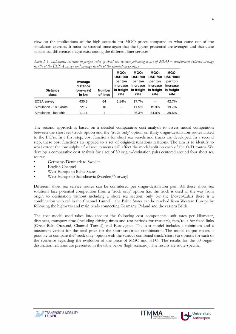
view on the implications of the high scenario for MGO prices compared to what came out of the simulation exercise. It must be stressed once again that the figures presented are averages and that quite substantial differences might exist among the different liner services. Table S.1. Estimated increase in freight rates of short sea services following a use of MGO – comparison between average results of the ECSA survey and average results of the simulation exercise

Distance class

Average distance

(one-way) in km

Number of lines

MGO: USD 200 per ton

Increase in freight

rate


Increase in freight

rate


Increase in freight

rate

MGO: USD 1000

per tonIncrease in freight

rate

ECSA survey 430.3 64 5.14% 17.7% - 42.7%

Simulation - 18.5knots 721.7 16 - 11.5% 15.9% 19.7%

Simulation - fast ship 1,111 1 - 26.3% 34.0% 39.6% The second approach is based on a detailed comparative cost analysis to assess modal competition between the short sea/truck option and the ‘truck only’ option on thirty origin-destination routes linked to the ECAs. In a first step, cost functions for short sea vessels and trucks are developed. In a second step, these cost functions are applied to a set of origin-destinations relations. The aim is to identify to what extent the low sulphur fuel requirements will affect the modal split on each of the O-D routes. We develop a comparative cost analysis for a set of 30 origin-destination pairs centered around four short sea routes: • Germany/Denmark to Sweden • English Channel • West Europe to Baltic States • West Europe to Scandinavia (Sweden/Norway) Different short sea service routes can be considered per origin-destination pair. All these short sea solutions face potential competition from a ‘truck only’ option (i.e. the truck is used all the way from origin to destination without including a short sea section: only for the Dover-Calais there is a combination with rail in the Channel Tunnel). The Baltic States can be reached from Western Europe by following the highways and main roads connecting Germany, Poland and the eastern Baltic. The cost model used takes into account the following cost components: unit rates per kilometer, distances, transport time (including driving times and rest periods for truckers), fees/tolls for fixed links (Great Belt, Oresund, Channel Tunnel) and Eurovignet. The cost model includes a minimum and a maximum variant for the total price for the short sea/truck combination. The model output makes it possible to compare the ‘truck only’ option with the various combined truck/short sea options for each of the scenarios regarding the evolution of the price of MGO and HFO. The results for the 30 origin-destination relations are presented in the table below (high scenario). The results are route-specific.

5

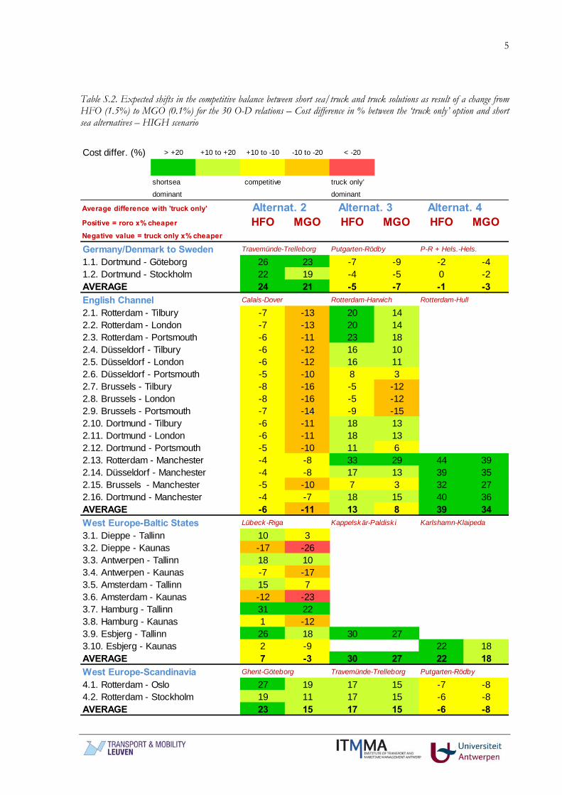
Table S.2. Expected shifts in the competitive balance between short sea/truck and truck solutions as result of a change from HFO (1.5%) to MGO (0.1%) for the 30 O-D relations – Cost difference in % between the ‘truck only’ option and short sea alternatives – HIGH scenario

Cost differ. (%) > +20 +10 to +20 +10 to -10 -10 to -20 < -20

shortsea competitive truck only'

dominant dominant

Average difference with 'truck only' Alternat. 2 Alternat. 3 Alternat. 4Positive = roro x% cheaper HFO MGO HFO MGO HFO MGONegative value = truck only x% cheaper

Germany/Denmark to Sweden Travemünde-Trelleborg Putgarten-Rödby P-R + Hels.-Hels.

1.1. Dortmund - Göteborg 26 23 -7 -9 -2 -41.2. Dortmund - Stockholm 22 19 -4 -5 0 -2AVERAGE 24 21 -5 -7 -1 -3English Channel Calais-Dover Rotterdam-Harwich Rotterdam-Hull

2.1. Rotterdam - Tilbury -7 -13 20 142.2. Rotterdam - London -7 -13 20 142.3. Rotterdam - Portsmouth -6 -11 23 182.4. Düsseldorf - Tilbury -6 -12 16 102.5. Düsseldorf - London -6 -12 16 112.6. Düsseldorf - Portsmouth -5 -10 8 32.7. Brussels - Tilbury -8 -16 -5 -122.8. Brussels - London -8 -16 -5 -122.9. Brussels - Portsmouth -7 -14 -9 -152.10. Dortmund - Tilbury -6 -11 18 132.11. Dortmund - London -6 -11 18 132.12. Dortmund - Portsmouth -5 -10 11 62.13. Rotterdam - Manchester -4 -8 33 29 44 392.14. Düsseldorf - Manchester -4 -8 17 13 39 352.15. Brussels - Manchester -5 -10 7 3 32 272.16. Dortmund - Manchester -4 -7 18 15 40 36AVERAGE -6 -11 13 8 39 34West Europe-Baltic States Lübeck-Riga Kappelskär-Paldisk i Karlshamn-Klaipeda

3.1. Dieppe - Tallinn 10 33.2. Dieppe - Kaunas -17 -263.3. Antwerpen - Tallinn 18 103.4. Antwerpen - Kaunas -7 -173.5. Amsterdam - Tallinn 15 73.6. Amsterdam - Kaunas -12 -233.7. Hamburg - Tallinn 31 223.8. Hamburg - Kaunas 1 -123.9. Esbjerg - Tallinn 26 18 30 273.10. Esbjerg - Kaunas 2 -9 22 18AVERAGE 7 -3 30 27 22 18West Europe-Scandinavia Ghent-Göteborg Travemünde-Trelleborg Putgarten-Rödby

4.1. Rotterdam - Oslo 27 19 17 15 -7 -84.2. Rotterdam - Stockholm 19 11 17 15 -6 -8AVERAGE 23 15 17 15 -6 -8

6

The main conclusions of the cost analysis can be divided in two groups. First of all, we can draw conclusions regarding the expected total cost changes per origin-destination relation. The use of MGO is expected to increase the transport prices particularly on the origin-destination relations with a medium or long short sea section. Such a price development might eventually trigger a shift from medium and long short sea routes to shorter short sea routes or a ‘truck only’ alternative without any short sea section. Secondly, we can draw conclusions regarding changes in the relative competitive position of the short sea/truck option versus the ‘truck only’ option when using MGO (0.1%) instead of HFO (1.5%) (per origin-destination relation):

1. On the trade lane between Germany/Denmark and Sweden, the Travemünde-Trelleborg ferry connection is competitive compared to the ‘truck only’ option. For the shorter short sea routes (alternatives 3 and 4), the price difference between the combined truck/short sea solution and the ‘truck only’ option diminishes when using MGO instead of HFO up to a level where the ‘truck only’ option becomes more competitive. The observed price gap, though small, can trigger a modal shift from sea to road in the high scenario.

2. The cross channel short sea business for manned truck/trailer combinations (Dover-Calais link) is likely to be hit hard by the use of MGO. The use of MGO could well imply a major traffic loss of manned truck/trailer combinations per vessel across the southern part of the English Channel with potentially negative implications on the ferry capacity for passenger transfers. The Rotterdam-Harwich short sea link shows the most competitive profile on all routes considered except for traffic flows to and from Manchester (price dominance of Rotterdam-Hull), but also here the use of MGO is expected to make its competitive position weaker. The narrowing of the price gap implies that the Rotterdam-Harwich short sea route moves towards a situation of increased competition with the truck/rail option. Such a development should raise great concern given longer truck distances on the already highly congested motorways in the southeast of the UK..

3. The transport connections between Western Europe and the Baltic States are expected to be heavily affected by the introduction of the new regulations on low sulphur requirements for vessels in the ECAs. While long-distance short sea transport succeeds in keeping a cost advantage over trucking on a number of O-D relations (see for example Hamburg-Tallinn), the ratio between the trucking price and the price for the truck/short sea combinations seriously deteriorates on most other routes. On the routes Dieppe-Kaunas and Amsterdam-Kaunas, short sea services are likely to completely lose their appeal to customers implying major modal shifts away from the Lübeck-Riga short sea link. On the routes Hamburg-Kaunas and Antwerp-Kaunas, the price disadvantage for the long-distance short sea solution becomes too high to guarantee a high competitiveness vis-à-vis trucking. Alternative short sea routes 3 and 4 remain competitive for connecting Esjberg to the Baltic States, but also there the price difference shrinks when introducing MGO.

4. At present, the short sea connections between the Benelux/Western Germany and Scandinavia (Sweden and Norway in particular) face rather limited competition from road haulage. The main competitor is the much shorter short sea link between Travemünde and Trelleborg (which involves much longer trucking distances). Nevertheless, the use of MGO is expected to narrow down the cost advantage of the long-distance short sea option to such an extent that some customers might start opting for trucking goods instead of using short sea services. More certain is that the use of MGO will trigger a shift from long-distance to short-distance short sea links. Hence, the Travemünde-Trelleborg route clearly overtakes the Ghent-Göteborg route to become the cheapest solution between Rotterdam and Stockholm, while the price gap also closes on the Rotterdam-Oslo link.

7

The results for the low scenario are slightly more positive for short sea services than in the high scenario, but still the use of MGO (0.1%) is expected to generate shifts from sea to road given the observed changes in the ratios between the truck prices and the truck/short sea prices. The logistics industry is sensitive to price changes. The observed shifts in price differences incurred when introducing MGO (0.1%) as a base fuel in the ECAs would undoubtedly lead to changes in the modal split at the expense of short sea services. We also indicated that on some routes shifts from long-distance to short-distance short sea routes are to be expected. Traffic losses for short sea services force short sea operators to reduce capacity, to downsize vessels deployed (leading to less economies of scale) and to limit frequency of their services. Lower frequencies and higher operational costs linked to smaller vessels further reduce the attractiveness/competiveness of the short sea option. If traffic losses reach a level no longer allowing the short sea operator to guarantee a minimum service frequency then a complete closure of the line is a probable outcome. In other words, even relatively small traffic losses (e.g. 10% to 20% less cargo) for existing short sea services can trigger a vicious cycle of capacity reduction and lower frequencies ultimately leading to a poorer position for short sea services and thus an unattractive market environment for investors. Vicious cycles characterized by the downsizing of short sea activities and the closures of lines can lead to an overall implosion of a short sea sub-market, leaving room to the ‘truck only’ option or short sea services on short or ultrashort distances to fill the gap in the market. What is the expected impact of the new requirements of IMO on external costs? The third section of the report focuses on the third research question: ‘What is the expected impact of the new requirements of IMO on external costs?’. This part of the report analyzes the external costs linked to the alternative routing options under three different scenarios regarding the implementation of low sulphur requirements:

- a reference scenario assuming the use of HFO with a 1% sulphur content - a simulation scenario assuming the use of HFO with a 0.5% sulphur content - a simulation scenario assuming the use of MDO with a 0.1% sulphur content. This scenario is

supposed to reflect the effect of the new requirement of IMO. The aim is to provide a detailed picture per route on the impact the implementation of the low sulphur emissions requirements is likely to have when comparing the truck only with the short sea/truck options. Using the methodology described in the report, we calculated the total marginal external costs for each route in detail for specific short sea vessels on five different routes for the 3 scenarios. For trucks and rail we used data from literature and assumed that they would remain the same in the reference and in the simulation scenarios. Using this information the marginal external costs for each origin-destination pair was calculated for 7 options

- the truck only option; where the English Channel is crossed using the Channel tunnel - the short sea/truck combination option in the reference case (1% S-HFO - the short sea/truck combination option in the simulation case (0.5%S-HFO), assuming no modal

shift as this does not require a change of type of fuel (HFO) and would hence not lead to large price increases

- the short sea/truck combination option in the simulation case (0.1%S-MDO), assuming no modal shift

- the short sea/truck combination option in the simulation case (0.1%S-MDO), assuming a modal shift of 10%



8

The analysis showed that - the requirements of the IMO indeed decrease emissions and hence external costs of short sea

shipping on its own - when considering a possible back shift of about 10-20% this effect could be completely mitigated.

Consider, for example, the route Lübeck-Trelleborg for trucks departing at Dortmund and arriving in Gotenburg. We assumed 88 trucks on the ship Mecklenburg-Vorpommern. In order to ease the comparison we assumed that all 88 trucks are leaving at Dortmund and arriving in Gotenburg. Of course, in reality a mixture of origin-destinations will be present. We then calculated total external costs for these trucks for the 7 options stated above. The results shown in the first 4 bars show the effects if no modal shift is assumed. For this origin-destination, the external costs are the higher for the truck only option than for the shipping option. Of course, in the simulations the total marginal external costs decrease. In the case of modal shift of 10% we assume that 79 trucks will remain on the ship, while 9 would use the land base alternative. The external cost of these 9 trucks is then added to the total external costs. This makes that when assuming a modal shift of 10% in the scenario with 0.1% sulphur the total marginal costs become higher than in the reference case with 1% sulphur. Figure S.1. Total marginal external costs (1000 euro) for Dortmund-Götenburg for the different modes – if modal shift

0

10

20

30

40

50

60

70

Road SSS - Ref SSS-SIM_0.5 nomodal shift

SSS-SIM_0.1 nomodal shift

SSS-SIM_0.1 10%modal shift



scenario

1000

Eur

o

SSSRoad

A similar picture is found back for all origin-destination pairs. For some of the origin-destinations, the truck only option leads to lower total external costs than the short sea/truck combinations. This is particularly the case when the trucks use the Channel tunnel, as the external costs of electric rail are very low. For other origin-destinations it should be noted that the external costs for vessels which also transport passengers are overestimated as we allocated the full external costs of short sea shipping completely to the freight transported. The importance of this assumption depends on the relative shares of passengers/freight transported. However, it is practically impossible to determine the share of external costs which need to be attributed to passengers and which part to freight traffic. Taking into account the assumptions, it can be seen that for 26% of the cases analysed, the gain in marginal external costs due to a decrease in sulphur content to 0.1% will deteriorate compared with the present situation if a modal shift of 10% occurs. If a modal shift of 20% occurs this is the case for almost

9

all origin-destinations. The analysis also shows that if we assume that a decrease in sulphur content to 0.5% would not lead to a modal shift, the total marginal external costs are lower for all routes than if sulphur content would equal 0.1% and a modal shift of about 20% would occur. In conclusion, the analysis showed clearly that– even when taking into account the assumptions made- when assessing the effects of a measure on external costs, one should also take into account that some costs are not removed, but shifted to other modes. In summary, the use of MGO (0.1%) is expected to have a negative effect on freight rates and the modal split on a large set of origin-destination relations. On some trade routes the short sea option might lose its appeal to customers. This will lead to traffic losses for the short sea option in favour of trucking or shorter short sea sections. Obviously, the use of MGO will have a positive impact on external costs generated by short sea vessels alone. Depending on the actual modal back shift the overall outcome for the environmental performance might well be negative.

10

TABLE OF CONTENTS

1. Background and research questions ............................................................................................................... 11

2. Methodology ...................................................................................................................................................... 13

3. What is the expected impact of the new requirements of IMO on costs and prices of short sea traffic in the ECAs? ............................................................................................................................................................... 14

3.1. The evolution of fuel prices ................................................................................................................... 14

3.2. Fuel costs for short sea vessels in the ECAs ....................................................................................... 20

3.3. Impact of fuel cost increases on freight rates...................................................................................... 26

4. What is the expected impact of the new requirements of IMO on the modal split in the ECAs?...... 29

4.1. Methodology ............................................................................................................................................. 29

4.2. Results from previous and ongoing studies ......................................................................................... 29

4.3. Stated preference method: survey results ............................................................................................. 31

4.4. Comparative cost/price analysis of the truck/short sea option versus the ‘truck only’ option.. 36

4.4.1. Cost functions for short sea vessels..................................................................................................... 36

4.4.2. Cost functions in road haulage ............................................................................................................. 38

4.4.3. Comparative cost analysis on origin-destination pairs...................................................................... 42

5. What is the expected impact of the new requirements of IMO on external costs? ............................... 56

5.1. Marginal external costs of shipping on selected routes ..................................................................... 56

5.2. Marginal external costs of trucks ........................................................................................................... 62

5.3. Marginal external cost of rail .................................................................................................................. 63

5.4. Marginal external cost of the selected routes – no modal shift. ....................................................... 63

5.5. Marginal external cost of the selected routes – if modal shift. ........................................................ 66

6. Conclusions and policy recommendations.................................................................................................... 70

11

1. Background and research questions The International Maritime Organization (IMO) is an agency of the United Nations which has been formed to promote maritime safety. The IMO ship pollution rules are contained in the International Convention on the Prevention of Pollution from Ships, known as MARPOL 73/78. On 27 September 1997, the MARPOL Convention has been amended by the 1997 Protocol, which includes Annex VI titled ‘Regulations for the Prevention of Air Pollution from Ships’. MARPOL Annex VI sets limits on NOx and SOx emissions from ship exhausts, and prohibits deliberate emissions of ozone depleting substances. The IMO emission standards are commonly referred to as Tier I, II and III standards. The Tier I standards were defined in the 1997 version of Annex VI, while the Tier II/III standards were introduced by Annex VI amendments adopted in October 2008. Two sets of emission and fuel quality requirements are defined by Annex VI: global requirements, and more stringent requirements applicable to ships in Emission Control Areas (ECA). An Emission Control Area can be designated for SOx and PM, or NOx, or all three types of emissions from ships. Before 2010, Annex VI to MARPOL 73/78 limited the sulphur content of marine fuel oil to 1.5% per mass and applied in designated SOx Emission Control Areas (SECA). The first SECA is the Baltic Sea entered into force on the 19 May 2006. The North Sea Area and the English Channel SECA entered into force on 22 November 2007. The SECA area represents about 0.3% of the world’s water surface. SECA does not include any other European waters such as the Irish Sea, Mediterranean Sea and Black Sea. New SECAs are expected to be adopted in the future based on certain criteria and procedures for designation of SECAs as given in MARPOL Appendix III to Annex VI. Figure 1.1. Geographical boundaries for the Baltic Sea SECA and the North Sea Area and the English Channel SECA

Directive 2005/33/EC largely mirrors MARPOL Annex VI, although the dates for implementation do not correlate exactly with those of Annex VI. The EU directive 2005/33/EC required ships to burn fuel oil with less than 1.5% sulphur in the North Sea SECA from 11 August 2007. There is a provision for the further reduction of sulphur content of marine fuels for vessels at berth in EU ports. This new provision entered into force date in 2010 with the maximum sulphur content from that date being 0.1%. The presence of sulphur in the marine fuels contributes to environmental pollution and other problems. As the sulphur in fuels burn, it will form SOx which is one of the pollutants to the environment especially in the formation of acid rain. Continued exposure over a long time changes the natural variety of plants and animals in an ecosystem. SO2 accelerates the decay of building materials and paints, including irreplaceable monuments, statues, and sculptures that are part of our nation's cultural heritage. The sulphur content in fuel oil has a large impact on the particle level in the exhaust gas.

12

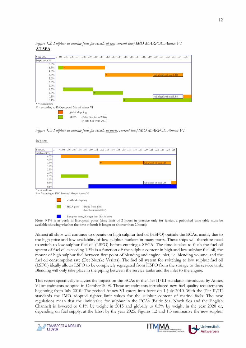
Figure 1.2. Sulphur in marine fuels for vessels at sea: current law/IMO MARPOL Annex VI AT SEA

Year 20.. .. .04 ..05 ..06 ..07 ..08 ..09 ..10 ..11 ..12 ..13 ..14 ..15 ..15 ..17 ..18 ..19 ..20 ..21 ..22 ..23 ..24 ..25Sulph.cont.%

5.0%4.5% *4.0%3.5% # sub check of avail..183.0%2.5%2.0%1.5% *1.0% #0.5% sub check of avail..180.1% #

* = current law# = according to IMO proposal Marpol Annex VI

global shipping

SECA (Baltic Sea from 2006)(North Sea from 2007)

Figure 1.3. Sulphur in marine fuels for vessels in ports: current law/IMO MARPOL Annex VI in ports

Year 20.. .. 4 ..05 ..06 ..07 ..08 ..09 ..10 ..11 ..12 ..13 ..14 ..15 ..15 ..17 ..18 ..19 ..20 ..21 ..22 ..23 ..24 ..25Sulph.cont.%

4.5%4.0% 3.5% # sub check of avail..183.0%2.5%2.0%1.5%1.0%0.5% sub check of avail..180.1% *

* = Actual Law# = According to IMO Proposal Marpol Annex VI

worldwide shipping

SECA ports (Baltic from 2005)(Northsea from 2007)

European ports, if longer than 2hrs in ports Note: 0.1% is at berth in European ports (time limit of 2 hours in practice only for ferries, a published time table must be available showing whether the time at berth is longer or shorter than 2 hours) Almost all ships will continue to operate on high sulphur fuel oil (HSFO) outside the ECAs, mainly due to the high price and low availability of low sulphur bunkers in many ports. These ships will therefore need to switch to low sulphur fuel oil (LSFO) before entering a SECA. The time it takes to flush the fuel oil system of fuel oil exceeding 1.5% is a function of: the sulphur content in high and low sulphur fuel oil, the mount of high sulphur fuel between first point of blending and engine inlet, i.e. blending volume, and the fuel oil consumption rate (Det Norske Veritas). The fuel oil system for switching to low sulphur fuel oil (LSFO) ideally allows LSFO to be completely segregated from HSFO from the storage to the service tank. Blending will only take place in the piping between the service tanks and the inlet to the engine. This report specifically analyses the impact on the ECAs of the Tier II/III standards introduced by Annex VI amendments adopted in October 2008. These amendments introduced new fuel quality requirements beginning from July 2010. The revised Annex VI enters into force on 1 July 2010. With the Tier II/III standards the IMO adopted tighter limit values for the sulphur content of marine fuels. The new regulations mean that the limit value for sulphur in the ECAs (Baltic Sea, North Sea and the English Channel) is lowered to 0.1% by weight in 2015 and globally to 0.5% by weight in the year 2020 or, depending on fuel supply, at the latest by the year 2025. Figures 1.2 and 1.3 summarize the new sulphur

13

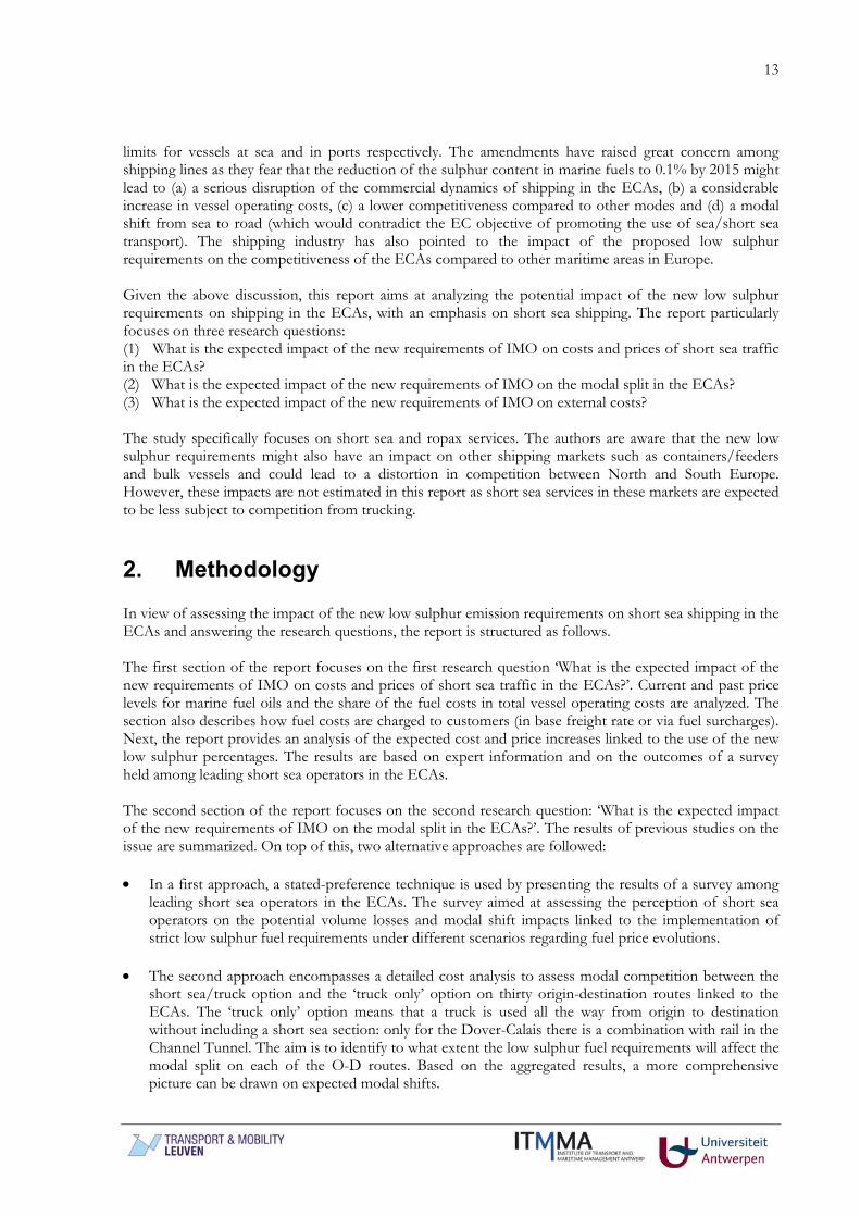
limits for vessels at sea and in ports respectively. The amendments have raised great concern among shipping lines as they fear that the reduction of the sulphur content in marine fuels to 0.1% by 2015 might lead to (a) a serious disruption of the commercial dynamics of shipping in the ECAs, (b) a considerable increase in vessel operating costs, (c) a lower competitiveness compared to other modes and (d) a modal shift from sea to road (which would contradict the EC objective of promoting the use of sea/short sea transport). The shipping industry has also pointed to the impact of the proposed low sulphur requirements on the competitiveness of the ECAs compared to other maritime areas in Europe. Given the above discussion, this report aims at analyzing the potential impact of the new low sulphur requirements on shipping in the ECAs, with an emphasis on short sea shipping. The report particularly focuses on three research questions: (1) What is the expected impact of the new requirements of IMO on costs and prices of short sea traffic in the ECAs? (2) What is the expected impact of the new requirements of IMO on the modal split in the ECAs? (3) What is the expected impact of the new requirements of IMO on external costs? The study specifically focuses on short sea and ropax services. The authors are aware that the new low sulphur requirements might also have an impact on other shipping markets such as containers/feeders and bulk vessels and could lead to a distortion in competition between North and South Europe. However, these impacts are not estimated in this report as short sea services in these markets are expected to be less subject to competition from trucking.

2. Methodology In view of assessing the impact of the new low sulphur emission requirements on short sea shipping in the ECAs and answering the research questions, the report is structured as follows. The first section of the report focuses on the first research question ‘What is the expected impact of the new requirements of IMO on costs and prices of short sea traffic in the ECAs?’. Current and past price levels for marine fuel oils and the share of the fuel costs in total vessel operating costs are analyzed. The section also describes how fuel costs are charged to customers (in base freight rate or via fuel surcharges). Next, the report provides an analysis of the expected cost and price increases linked to the use of the new low sulphur percentages. The results are based on expert information and on the outcomes of a survey held among leading short sea operators in the ECAs. The second section of the report focuses on the second research question: ‘What is the expected impact of the new requirements of IMO on the modal split in the ECAs?’. The results of previous studies on the issue are summarized. On top of this, two alternative approaches are followed: • In a first approach, a stated-preference technique is used by presenting the results of a survey among

leading short sea operators in the ECAs. The survey aimed at assessing the perception of short sea operators on the potential volume losses and modal shift impacts linked to the implementation of strict low sulphur fuel requirements under different scenarios regarding fuel price evolutions.

• The second approach encompasses a detailed cost analysis to assess modal competition between the

short sea/truck option and the ‘truck only’ option on thirty origin-destination routes linked to the ECAs. The ‘truck only’ option means that a truck is used all the way from origin to destination without including a short sea section: only for the Dover-Calais there is a combination with rail in the Channel Tunnel. The aim is to identify to what extent the low sulphur fuel requirements will affect the modal split on each of the O-D routes. Based on the aggregated results, a more comprehensive picture can be drawn on expected modal shifts.

14

The third section of the report focuses on the third research question: ‘What is the expected impact of the new requirements of IMO on external costs?’. Using the results of the second section, this part of the report will analyze the external costs (such as congestion, air pollutants,etc.) linked to the alternative routing options for three scenarios regarding the implementation of low sulphur requirements:

- a reference scenario assuming the use of 1% sulphur HFO - a simulation scenario assuming the use of 0.5% sulphur HFO - a simulation scenario assuming the use of 0.1% sulphur HFO

The aim is to provide a detailed picture per route on the impact the implementation of the low sulphur emissions requirements is likely to have on the total external cost balance, taking into account possible modal shifts.

3. What is the expected impact of the new requirements of IMO on costs and prices of short sea traffic in the ECAs?

3.1. The evolution of fuel prices Bunker prices constantly fluctuate due to market forces and the cost of crude oil. Peaks and lows in the oil price have been moderate most of the time, with the several oil crises as notably exceptions. The oil market has witnessed extreme volatility during 2008. Since early 2007, the oil price rapidly rose to reach a peak in the middle of 2008. The oil price abruptly changed thereafter: the crude oil price (Dated Brent) amounted to USD 92 per barrel in January 2008, reached USD 145 per barrel in July 2008 and fell back to USD 40 per barrel, on average, in December 2008, losing more than 70% of its value. Since early 2009 the oil price shows a moderate increasing trend from a level of USD 42 per barrel in February 2009 to USD 69 per barrel in June 2009. Figure 3.1. The index evolution of crude oil, diesel oil and other oil products

Source: based on Market Observatory of Energy (2009)

15

The prices of oil products also fluctuated extensively as compared to historical standards, reaching the peak in July 2008 and sharply falling afterwards. The fluctuations of main end-user petroleum product prices, such as diesel oil used by trucks, are typically less pronounced as crude oil price comprises only part of the final price, the rest being largely determined by the application of taxes. The Market Observatory for Energy (2009) reports that the share of taxation (indirect taxes + VAT) in the end-consumer price of automotive diesel oil is decreasing when the crude price and the net product prices are increasing and, conversely, it is increasing when the crude price and the net product prices are decreasing. In January 2009, the taxation share ranged from 45% in Cyprus to 66% in the UK with most EU Member States fluctuating around 55%. In July 2008, when fuel prices peaked, the taxation share ranged from 33% in Cyprus to 53% in the United Kingdom. Despite the sudden drop in fuel prices in the second half of 2008, the end-consumer price (including taxes) for automotive diesel oil in January 2009 still remained higher than in January 2003 by about 15% (figure 3.1). The fact that the price evolution of automotive diesel oil is not in line with the price evolution of crude oil may be due to constraints in the production capacity in the refining industry. Large differences in automotive diesel prices can be observed among Member States, mainly due to differences in taxation regimes (figure 3.2). Figure 3.2. Differences in diesel and fuel prices among European countries – situation in July 2008 (peak in fuel prices)

Source: GfK Geomarketing The price evolution for marine fuel oils is more in line with the oil price and price differences among bunker ports are typically quite moderate. But also here, bunkering decisions are impacted by relative price premiums arising as a result of different fiscal policies across countries and regions, especially in terms of fuel taxes. Large amounts of bunker fuel are consumed each year by the world fleet of cargo and commercial vessels as well as the military ones. About 80% of the total bunker fuel relates to heavy fuel oil. Heavy Fuel Oil (HFO) mainly consists of residual refinery streams from the distillation or cracking units in the refineries. The type of HFO is mainly defined by the crude quality and the refinery process. High sulphur crude will result in a high sulphur HFO. Other bunker fuels than the HFO are the marine

16

diesel oil (MDO) and the marine gas oil (MGO). These are distillates from the refinery process with much lower viscosity and lower sulphur content. In summary the following fuels can be used for vessels (see table 3.1 for more technical details): • Residual oil: it is the heaviest fraction of the distillation of crude oil, with high viscosity (=> pre-

heating necessary => used only in large ships) and high concentration of pollutants (e.g. sulphur). Its combustion produces a much darker smoke than other fuels and it needs specific temperature for storage and pumping. Due to these drawbacks, it is also the cheapest liquid fuel on the market.

• IFO 380 (Intermediate Fuel Oil) is a mix of 98% of residual oil and 2% of distillate oil. • IFO 180 (Intermediate Fuel Oil) is a mix of 88% of residual oil and 12% of distillate oil. Due to the

higher content in distillate oil, IFO 180 is more expensive than IFO 380. • MDO (Marine Diesel Oil) mainly consists of distillate oil and has a lower sulphur content than the

three fuels described above. • MGO (Marine Gas Oil) is pure distillate oil and has the lowest sulphur content. A large part of the difference between HFO (Heavy Fuel Oil) and MDO (Marine Diesel Oil) is related to sulphur which together with water forms particulates. The removal of sulphur from residual fuel oil prior to usage is technically feasible, but the economics of residue desulphurisation are not very attractive. Uncertainty of price and the often negative refinery margin limit are obstacles to investments. Distillate is an alternative fuel which can be supplied with a low or zero sulphur content. Whilst HFO is the untreated component of crude oil remaining after vacuum distillation, distillate undergoes several refinery processes all of which utilize refinery energy to produce the finished product. Thus it is important to consider both the specific energy of the respective fuels and the energy required to process the products. This will be discussed in more detail in the part on external costs. Under the old EC Directive 1999/32, all marine distillates were defined as (marine) gas oil, making no distinction between various grades of marine diesel oils (MDO) and marine gas oils (MGO). Since its application date in July 2000, ships were only allowed to burn marine distillates with a maximum Sulphur content of 0.2% while sailing within EU territory. Directive 2005/33/EC, however, makes a distinction between MDO and MGO. The maximum allowable Sulphur content for MGO fell to 0.1% after January 2008. But for MDO, the limit has been raised from 0.2% to 1.5%, which means ships are again free to buy and use MDO with up to 1.5% Sulphur. Costs are incurred when ships have to switch from residual fuels (IFO 380, average sulphur content of 2.67%) to marine distillate fuels (average sulphur content of 0.65%) in order to meet the minimum regulatory requirements. Table 3.1. Specifications of the most common marine fuels

Industrial name ISO name Composition ISO Specification World averagesulphur weight %

Intermediate Fuel Oil MRG35 98% residual oil 5% (*) 2.67%380 (IFO 380) 2% distillate oil

Intermediate Fuel Oil RME25 88% residual oil 5% (*) 2.67%180 (IFO 180) 12% distillate oil

Marine Diesel Oil (MDO) DMB Distillate oil with trace 2% 0.65%of residual oil

Marine Gas Oil (MGO) DMA 100% destillate oil 1.5% 0.38%

(*) IMO regulation capping sulphur at 4.5% supercided ISO specification Source: ICCT (2007)

17

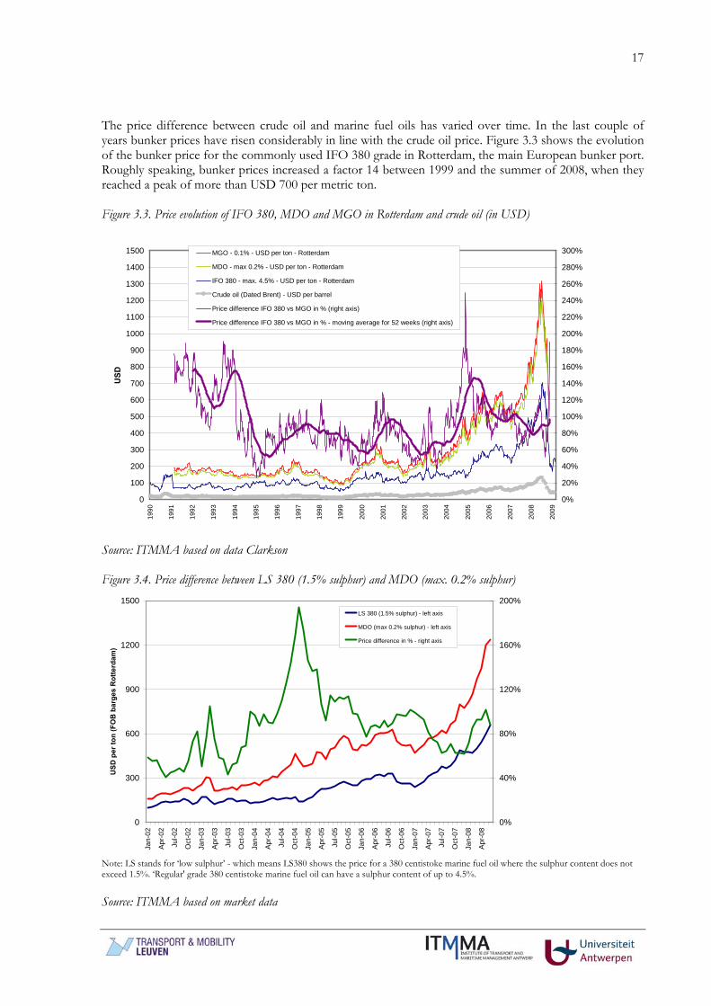
The price difference between crude oil and marine fuel oils has varied over time. In the last couple of years bunker prices have risen considerably in line with the crude oil price. Figure 3.3 shows the evolution of the bunker price for the commonly used IFO 380 grade in Rotterdam, the main European bunker port. Roughly speaking, bunker prices increased a factor 14 between 1999 and the summer of 2008, when they reached a peak of more than USD 700 per metric ton. Figure 3.3. Price evolution of IFO 380, MDO and MGO in Rotterdam and crude oil (in USD)

0

100

200

300

400

500

600

700

800

900

1000

1100

1200

1300

1400

1500

1990

1991

1992

1993

1994

1995

1996

1997

1998

1999

2000

2001

2002

2003

2004

2005

2006

2007

2008

2009

USD

0%

20%

40%

60%

80%

100%

120%

140%

160%

180%

200%

220%

240%

260%

280%

300%MGO - 0.1% - USD per ton - Rotterdam

MDO - max 0.2% - USD per ton - Rotterdam

IFO 380 - max. 4.5% - USD per ton - Rotterdam

Crude oil (Dated Brent) - USD per barrel

Price difference IFO 380 vs MGO in % (right axis)

Price difference IFO 380 vs MGO in % - moving average for 52 weeks (right axis)

Source: ITMMA based on data Clarkson Figure 3.4. Price difference between LS 380 (1.5% sulphur) and MDO (max. 0.2% sulphur)

0

300

600

900

1200

1500

Jan-

02

Apr

-02

Jul-0

2

Oct

-02

Jan-

03

Apr

-03

Jul-0

3

Oct

-03

Jan-

04

Apr

-04

Jul-0

4

Oct

-04

Jan-

05

Apr

-05

Jul-0

5

Oct

-05

Jan-

06

Apr

-06

Jul-0

6

Oct

-06

Jan-

07

Apr

-07

Jul-0

7

Oct

-07

Jan-

08

Apr

-08

USD

per

ton

(FO

B b

arge

s R

otte

rdam

)

0%

40%

80%

120%

160%

200%LS 380 (1.5% sulphur) - left axis

MDO (max 0.2% sulphur) - left axis

Price difference in % - right axis

Note: LS stands for ‘low sulphur’ - which means LS380 shows the price for a 380 centistoke marine fuel oil where the sulphur content does not exceed 1.5%. ‘Regular' grade 380 centistoke marine fuel oil can have a sulphur content of up to 4.5%. Source: ITMMA based on market data

18

Figures 3.3 reveals that the price difference between IFO 380 and MGO (0.1% sulphur) fluctuates strongly in time (30% to 250% price difference). The moving annual average ranges from 52% to 155% and the long term average amounts to 93% (period 1990-2008). Figure 3.4 provides more details on the price evolution for various grades of marine fuels with low sulphur contents between 2002 and the summer of 2008. The price difference between LS 380 and MDO fluctuates between 40% and 190%, with a long term average of 87%. In other words, the specified MDO is on average 87% more expensive than LS 380. Overall the cost of marine distillate fuels is about twice what residual fuels costs due to increasing demand and the cost of the desulphurization process. These are long-term averages. Table 3.2. Recent bunker price evolution of IFO 380, LS 380 and MGO in Rotterdam (USD per ton, monthly averages).

IFO 380 max 4.5%

LS 380 max 1.5%

MGO 0.1%

Price difference MGO vs IFO 380

Price difference LS 380 vs IFO 380

Price difference MGO vs LS 380

June-08 635 695 1265 99.2% 9.4% 82.0%

January-09 229.5 283.5 458.5 99.8% 23.5% 61.7%February-09 240 285 406.5 69.4% 18.8% 42.6%

March-09 241.5 284 412 70.6% 17.6% 45.1%April-09 275.5 321.5 446.5 62.1% 16.7% 38.9%May-09 326.5 370.5 480 47.0% 13.5% 29.6%

June-09 381 417 570 49.6% 9.4% 36.7%July-09 379.5 410 534 40.7% 8.0% 30.2%

December 28, 2009 433.5 460.5 630.5 45.4% 6.2% 36.9% Note: MGO indications can be either 0.2% or 0.1% sulphur. Higher end of prices 0.1% sulphur product - most quotes are for 0.1%. Source: based on data Bunkerworld A more recent cost comparison difference is provided in table 3.2. It can be concluded that the price difference between regular IFO 380 and LS 380 is quite small. The gap has narrowed in recent months to only 6%. However, a shift from LS 380 with a maximum sulphur content of 1.5% to MGO with a maximum sulphur content of 0.1% has much larger implications on the bunker costs: in the summer of 2008 the difference reached 82% which is in line with the values of figures 3.3 and 3.4. However, in recent months it is fluctuating around 30 to 45%. The price gap between regular IFO 380 and MGO reached only 45.4% in July 2009. Given the long-term evolution of the price difference (i.e. long-term average price gap of 93% as depicted by figure 3.3), this small price gap of the last months must be seen as a lower boundary. In other words, the compulsory use of low sulphur fuel of maximum 0.1% in ECAs by 2015 would lead to a significant increase in the bunker costs for shipping lines. There are five points to be made in this respect. First of all, it is very difficult to forecast the evolution of the fuel prices and with it the future price gaps between IFO, MDO and MGO. As mentioned earlier, the oil price is a determining factor together with the demand/supply balance for each of the marine fuel grades. Whether the global refining industry is willing and able to produce the required volume of distillates implied by the regulation is an important issue. Several sources underline that the oil industry will be able to process sufficient low-sulphur fuel until 2015 in order to meet shipping’s requirement within the ECAs (see e.g. Swedish Maritime Administration, 2009:28). Oil company BP argues that there are adequate avails of lower sulphur residual material but at increasing prices due to processes of re-blending, additional blending, sweeter crude oil slates and residual desulphurisation. EC–DG Environment (2002) concludes that to supply fuels with lower sulphur content specifications than 1.5%, the European refining industry would need to invest in additional middle distillate desulphurisation capacity. This capacity is already fully utilized due to the progressive reduction

19

in sulphur content of on road diesel. Based on the cost of adding additional middle distillate desulphurisation capacity, the price premia for producing lower sulphur content has been estimated as 14 to 21 euro per ton for 0.1% sulphur (figures for 2002). In 2005, a study on the evaluation of low sulfur marine fuel availability commissioned by the Port of Los Angeles was one of the first to warn for a potential shortage of low sulphur fuels in world bunker ports. The study concluded that the lowest sulphur content readily available (<0.2%) is not guaranteed, it may only be supplied if the lower sulphur content is specifically requested. And, lower sulfur marine distillate may be available upon request at certain ports, but not guaranteed to be available on a constant basis or regionally. Second, the impact of oil price increases on the bunker cost for shipping is much more direct than in the case of trucking as a large part of the diesel price for trucks consists of taxes. Third, the trucking industry shows much more flexibility in adapting to changing rules regarding emissions. One of the reasons is that trucks are amortized over a period of 3 to 4 years, while in shipping vessels have a much longer lifecycle. In other words, it only takes a few years for the trucking industry to renew a fleet, while in shipping much more time is needed. The result is that energy efficiency gains due to new technologies develop rather fast in the trucking industry, but need more implementation time in the shipping industry. Fourth, it is important to note that the cost increase is not the only aspect. Shipowners will also benefit in technical terms from using low sulphur fuels. For instance, apart from causing less pollution to the environment, distillate fuels also have higher thermal value which reduces engine wear (requiring less frequent maintenance) and lowers fuel consumption. Distillate fuel has a lower density than residual fuel oil and it also has a higher energy content (HFO circa 40MJ/kg, Diesel Oil circa 42MJ/kg). Also, distillate fuel is of higher quality which results in less sludge on board and thereby benefits the operators who are finding it increasingly difficult to dispose sludge on shore. Improvement in the vessel’s engine maintenance is expected to help mitigate the impacts of increased fuel costs. Fifth, alternative measures to reduce sulphur emissions are also allowed (in the ECAs and globally), such as through the use of scrubbers. For example, instead of using low sulphur fuel in ECAs, ships can fit an exhaust gas cleaning system (EGCS) or use any other technological method to limit SOx emissions to ≤ 6 g/kWh. Since scrubber technology is evolving rapidly, it is not entirely clear whether the costs of the use of scrubbers is competitive to the use of expensive low sulphur fuel. The development of stack-scrubbers for ships is still at an early stage and local authorities may prohibit discharging waste streams from scrubbers in ports and estuaries. The disposal problem seriously undermines future large-scale deployment of scrubbers. There is also a space issue when retrofitting scrubbers to existing vessels linked to the engine casing and acid-proof coated tanks. Krystallon (2008) argues there is a net CO2 benefit from the use of high sulphur fuel oil and scrubbers. Although the scrubber incurs CO2 emissions for neutralisation and for scrubber additional fuel consumption, this would be significantly less than the CO2 emitted by the additional refinery processing of the distillate. On-going development of scrubbing technology will inevitably lead to lower energy demand and may in the future be capable of scrubbing out other gases such as nitrogen oxides (NOx). By the use of scrubbing and other after-treatment technologies, the ‘zero emissions’ ship capable of consuming available fuels is a distinctly feasible long term objective. Overall, we believe that the effect of the new Annex VI agreement may be quite costly for the participants in the shipping industry. Based on historical price differences, the use of MGO (0.1%) could well imply a cost increase per ton of bunker fuel of on average 80 to 100% (long-term) compared to IFO 380 and 70 to 90% compared to LS 380 grades (1.5%). This conclusion is in line with previous studies (see e.g. Skogs Industrierna, 2009). The price curve when moving from 1.5% sulphur content (LS 380) to 0.1% does not show a linear shape. A shift from 1.5% to 0.5% sulphur content represents an estimated cost increase of 20 to 30%. The price effect when moving from 0.5% to 0.1% sulphur content is much more substantial with a 50% to 60% bunker cost increase. The combined effect of these percentages corresponds to a total cost increase of 70 to 90% compared to LS 380 grades (1.5%).

20

The next section will assess the ramifications of these price increases on the total ship costs of vessels operating in the waters of the ECAs and thus also on the pricing strategies of shipping lines.

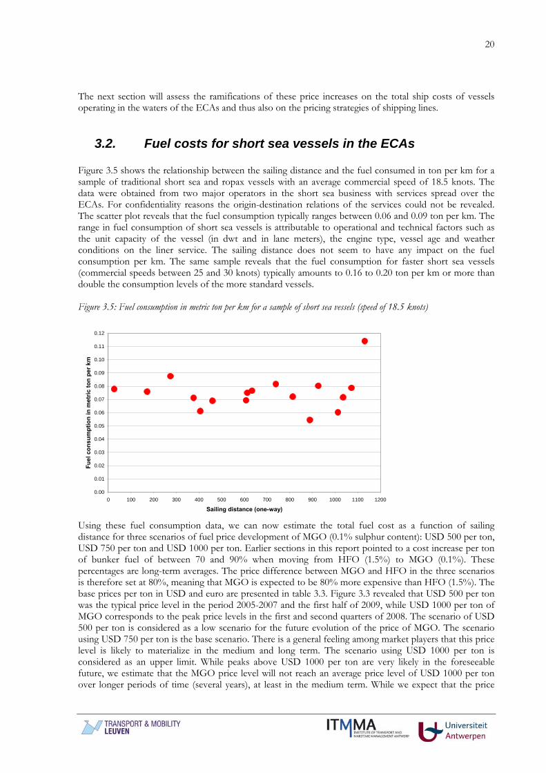
3.2. Fuel costs for short sea vessels in the ECAs Figure 3.5 shows the relationship between the sailing distance and the fuel consumed in ton per km for a sample of traditional short sea and ropax vessels with an average commercial speed of 18.5 knots. The data were obtained from two major operators in the short sea business with services spread over the ECAs. For confidentiality reasons the origin-destination relations of the services could not be revealed. The scatter plot reveals that the fuel consumption typically ranges between 0.06 and 0.09 ton per km. The range in fuel consumption of short sea vessels is attributable to operational and technical factors such as the unit capacity of the vessel (in dwt and in lane meters), the engine type, vessel age and weather conditions on the liner service. The sailing distance does not seem to have any impact on the fuel consumption per km. The same sample reveals that the fuel consumption for faster short sea vessels (commercial speeds between 25 and 30 knots) typically amounts to 0.16 to 0.20 ton per km or more than double the consumption levels of the more standard vessels. Figure 3.5: Fuel consumption in metric ton per km for a sample of short sea vessels (speed of 18.5 knots)

0.00

0.01

0.02

0.03

0.04

0.05

0.06

0.07

0.08

0.09

0.10

0.11

0.12

0 100 200 300 400 500 600 700 800 900 1000 1100 1200

Sailing distance (one-way)

Fuel

con

sum

ptio

n in

met

ric to

n pe

r km

Using these fuel consumption data, we can now estimate the total fuel cost as a function of sailing distance for three scenarios of fuel price development of MGO (0.1% sulphur content): USD 500 per ton, USD 750 per ton and USD 1000 per ton. Earlier sections in this report pointed to a cost increase per ton of bunker fuel of between 70 and 90% when moving from HFO (1.5%) to MGO (0.1%). These percentages are long-term averages. The price difference between MGO and HFO in the three scenarios is therefore set at 80%, meaning that MGO is expected to be 80% more expensive than HFO (1.5%). The base prices per ton in USD and euro are presented in table 3.3. Figure 3.3 revealed that USD 500 per ton was the typical price level in the period 2005-2007 and the first half of 2009, while USD 1000 per ton of MGO corresponds to the peak price levels in the first and second quarters of 2008. The scenario of USD 500 per ton is considered as a low scenario for the future evolution of the price of MGO. The scenario using USD 750 per ton is the base scenario. There is a general feeling among market players that this price level is likely to materialize in the medium and long term. The scenario using USD 1000 per ton is considered as an upper limit. While peaks above USD 1000 per ton are very likely in the foreseeable future, we estimate that the MGO price level will not reach an average price level of USD 1000 per ton over longer periods of time (several years), at least in the medium term. While we expect that the price

21

evolution for MGO in the foreseeable future will most likely fluctuate around the base scenario, we will mainly present the results of the low and high scenario in view of providing an upper and lower limit to the expected impact of the shift from HFO to MGO on ship costs, freight rates and modal competition between short sea/truck combinations and the ‘truck only’ option. Table 3.3. Price per ton of HFO and MGO in the three scenarios

HFO (1.5%)LOW

MGO (0.1%)LOW

HFO (1.5%)BASE

MGO (0.1%)BASE

HFO (1.5%)HIGH

MGO (0.1%)HIGH

USD 278 500 417 750 556 1000Euro 193 348 290 521 386 695 Note: average exchange rate of 2008 (yearly average) Figure 3.6: Total fuel costs per trip for the three scenarios

0

5000

10000

15000

20000

25000

30000

35000

40000

45000

50000

55000

0 50 100

150

200

250

300

350

400

450

500

550

600

650

700

750

800

850

900

950

1000

1050

1100

1150

1200

Sailing distance in km per trip

Tota

l fue

l cos

ts p

er tr

ip (i

n eu

ro)

HFO (1.5%)BASE

MGO (0.1%)BASE

HFO (1.5%)LOW

MGO (0.1%)LOW

HFO (1.5%)HIGH

MGO (0.1%)HIGH

10425 euro

Situation for roro/ropax vessel consuming 0.06 ton per km (18.5 knots)

16680 euro

6950 euro

3475

24 hourssailing time

35.5 hourssailing time

22

Figure 3.6: Total fuel costs per trip for the three scenarios (continued)

0

5000

10000

15000

20000

25000

30000

35000

40000

45000

50000

55000

60000

65000

70000

75000

80000

0 50 100

150

200

250

300

350

400

450

500

550

600

650

700

750

800

850

900

950

1000

1050

1100

1150

1200


Tota

l fue

l cos

ts p

er tr

ip (i

n eu

ro)

MGO (0.1%)BASE

MGO (0.1%)BASE

HFO (1.5%)LOW

MGO (0.1%)LOW

HFO (1.5%)HIGH

MGO (0.1%)HIGH

15638 euro

Situation for roro/ropax vessel consuming 0.09 ton per km (18.5 knots)

25020 euro

10425 euro

5213


35.5 hourssailing time

0

10000

20000

30000

40000

50000

60000

70000

80000

90000

100000

110000

120000

130000

140000

150000

160000

0 50 100

150

200

250

300

350

400

450

500

550

600

650

700

750

800

850

900

950

1000

1050

1100

1150

1200


Tota

l fue

l cos

ts p

er tr

ip (i

n eu

ro)

HFO (1.5%)BASE

MGO (0.1%)BASE

HFO (1.5%)LOW

MGO (0.1%)LOW

HFO (1.5%)HIGH

MGO (0.1%)HIGH 31275 euro

Situation for fast roro/ropax vessel consuming 0.18 ton per km (27 knots)

50040 euro

20850 euro

10425


23

Figure 3.6 gives an indication of the total fuel costs for short sea vessels. Three typical cases are considered: a short sea vessel consuming 0.06 ton per km and sailing at 18.5 knots, a short sea vessel consuming 0.09 ton per km and sailing at 18.5 knots and a fast short sea vessel consuming 0.18 ton per km and sailing at 27 knots. On long-distance short sea services of 1,200 km, the additional fuel costs linked to the use of MGO (0.1%) in the base scenario range between 16,680 and 50,040 euro for a single trip (depending on vessel speed and type). A comprehensive interpretation of these absolute figures requires a better insight in the share of fuel costs in total operating costs of short sea vessels sailing in the ECAs. An increase in the bunker oil price has an upward effect on costs. In the tanker market many vessels are on time charter where bunkers are paid by the charterer. For liner shipping activities, ship fuel is a considerable expense. Especially 2007 till the autumn of 2008 saw a succession of container shipping lines reporting on the effect of the price increases on their accounting bottom lines1. Ship costs include the vessel operating costs, vessel capital costs, bunker costs and port charges. A calculation of total operating costs of vessels thus requires data on variables such as capital costs, daily running costs and port dues2, administrative costs, etc. The total operating costs per unit transported (e.g. a truck/trailer combination or an unmanned trailer) depend also on the vessel utilization on the route considered. However, there are no reports available on the share of fuel costs in the total operating costs of short sea vessels. Therefore, we base ourselves on a sample of 15 short sea liner services operated in the ECAs. The share of bunker costs in total ship costs for this sample of vessels ranged between 26% and 48% in 2008 (figure 3.7). Total ship costs are the sum of bunker costs and vessel costs (i.e. the daily time charter rate for a vessel of that type and capacity). The share of fuel costs depends on the applicable bunker cost per ton: it will be high when fuel prices are high and lower when fuel prices are low. The average fuel cost for HFO (1.5%) in 2008 amounted to USD 490 per ton, which is close to the high scenario (USD 556 per ton, see table 3.3). The sample does not include fast short sea vessels with a commercial speed of 25 to 30 knots. For these vessels fuel costs are estimated to have reached between 38% and 60% in 2008 (based on data from market players)3.

1 Notteboom & Vernimmen (2009) demonstrated that a doubling of the bunker costs from USD 250 per ton (IFO 380) to USD 450 per ton has a very important impact on the costs faced by container shipping lines. Container vessels sailing at 24 knots incur a bunker cost that represents nearly 60% of the total ship costs and up to 40% of the total costs. At a bunker cost of USD 250 per ton these figures are 44% and 28% respectively. Bunker costs in container shipping typically accounted for two-thirds of voyage operating costs in late 2007. Container shipping lines are using fuel surcharges to recoup some of the increased costs in an attempt to pass the costs on to the customer through variable charges. 2 Port dues include towage dues, pilotage dues, traffic control system dues, reporting dues, (un)mooring dues, berth dues and tonnage dues. Given the frequency of sailings most roro vessels do not require a pilot on board when entering the port. Also, quite a number of roro and ropax vessels have bow thrusts which improves manoeuvreability and avoids the use of tug boats. 3 It was demonstrated earlier that the fuel consumption in ton per km for fast vessels is more than double the fuel consumption of more traditional roro and ropax vessels. The other ship costs are however also higher.

24

Figure 3.7. Share of bunker costs in total ship costs (in %) for a sample of liner services

0%

5%

10%

15%

20%

25%

30%

35%

40%

45%

50%

0 100 200 300 400 500 600 700 800 900 1000 1100 1200

Shar

e of

bun

ker

cost

s in

tota

l ves

sel o

pera

ting

cost

s (in

%)

Sailing distance (one-way)

Situation 2008 for roro/ropax vessels sailing at 18.5 knotsFuel HFO (1.5%) with average bunker price in 2008 of USD 490 per ton or 350 euro per ton

Using the same sample of short sea services, we can now estimate the share of fuel costs in total ship costs for different scenarios regarding fuel price per ton (table 3.4). For confidentiality reasons, the origin-destinations pairs are not listed in the table, only the service’s sub-market and distance class. When using HFO (1.5%) the average share of bunkers in total ship costs amounts to 23.8% in the low scenario (with lower and upper limits 16.2% for ultra-short routes and 33.5% respectively), 31.9% in the base scenario (22.5% to 43.1%) and nearly 38.3% in the high scenario (28% to 50%). The use of MGO would increase the average share of fuel costs to 35.9%, 45.5% and 52.5% respectively. Table 3.5 provides an overview of the increase in total ship costs when shifting from HFO (1.5%) to MGO. The impact on shipping lines’ cost base would be considerable: a 25.5% increase in ship costs for the base scenario and even 30.6% on average for the high scenario with for a number of routes peaks of 40%. These figures only relate to vessels with an average commercial speed of 18.5 knots. The average ship cost increase for fast short sea ships (25 to 30 knots on average) is estimated at 29% for the low scenario and even 40% (ranging from 31% to 47%) for the high scenario.

25

Table 3.4. Share of bunker costs in total ship costs for the three scenarios and for two fuel types: HFO (1.5%) and MGO (0.1%) – see table 3.3 for fuel costs per ton – short sea vessels with an average commercial speed of 18.5 knots

Share of bunker costs in total operating costs (bunker+vessel costs)

Sub-market Distance class

HFO (1.5%)LOW

MGO (0.1%)LOW

HFO (1.5%)BASE

MGO (0.1%)BASE

HFO (1.5%)HIGH

MGO (0.1%)HIGH

Route 1 UK/LH-H range <-> Baltic >750km 22.6% 34.4% 30.5% 44.1% 36.9% 51.2%Route 2 UK/LH-H range <-> Baltic >750km 23.3% 35.3% 31.3% 45.1% 37.8% 52.2%Route 3 UK/LH-H range <-> Baltic >750km 23.7% 35.8% 31.8% 45.6% 38.3% 52.8%Route 4 UK <-> LH-H range 400-750km 29.0% 42.3% 38.0% 52.4% 44.9% 59.5%Route 5 UK/LH-H range <-> Baltic >750km 26.9% 39.8% 35.6% 49.9% 42.4% 57.0%Route 6 UK/LH-H range <-> Baltic 400-750km 24.0% 36.2% 32.1% 46.0% 38.7% 53.1%Route 7 UK/LH-H range <-> Baltic 400-750km 17.6% 27.8% 24.3% 36.6% 30.0% 43.5%Route 8 UK/LH-H range <-> Baltic 400-750km 26.4% 39.2% 35.0% 49.2% 41.8% 56.3%Route 9 Intra-Baltic >750km 25.6% 38.3% 34.1% 48.2% 40.8% 55.4%Route 10 Intra-Baltic >750km 33.5% 47.5% 43.1% 57.7% 50.2% 64.4%Route 11 Intra-Baltic 400-750km 23.0% 35.0% 31.0% 44.7% 37.4% 51.9%Route 12 Intra-Baltic 400-750km 27.3% 40.4% 36.1% 50.4% 42.9% 57.5%Route 13 Intra-Baltic 400-750km 21.6% 33.2% 29.3% 42.7% 35.5% 49.8%Route 14 Intra-Baltic Ultra-short 16.2% 25.9% 22.5% 34.3% 27.9% 41.1%Route 15 Intra-Baltic Ultra-short 16.9% 26.9% 23.5% 35.5% 29.0% 42.3%Average 23.8% 35.9% 31.9% 45.5% 38.3% 52.5%Standard deviation 4.6% 5.9% 5.6% 6.4% 6.1% 6.5%High 33.5% 47.5% 43.1% 57.7% 50.2% 64.4%Low 16.2% 25.9% 22.5% 34.3% 27.9% 41.1% Note: LH-H = ports in the Le Havre-Hamburg range, a port range containing all seaports along the coastline between Hamburg in Germany and Le Havre in France. Table 3.5. Increase in total ship costs as a result of the use of MGO (0.1%) – short sea vessels with an average commercial speed of 18.5 knots

Total costs increase per trip (in %)

Sub-market Distance classScenario

LOWScenario

BASEScenario

HIGHRoute 1 UK/LH-H range <-> Baltic >750km 18.1% 24.4% 29.5%Route 2 UK/LH-H range <-> Baltic >750km 18.6% 25.0% 30.2%Route 3 UK/LH-H range <-> Baltic >750km 18.9% 25.4% 30.6%Route 4 UK <-> LH-H range 400-750km 23.2% 30.4% 35.9%Route 5 UK/LH-H range <-> Baltic >750km 21.5% 28.5% 33.9%Route 6 UK/LH-H range <-> Baltic 400-750km 19.2% 25.7% 30.9%Route 7 UK/LH-H range <-> Baltic 400-750km 14.1% 19.5% 24.0%Route 8 UK/LH-H range <-> Baltic 400-750km 21.1% 28.0% 33.4%Route 9 Intra-Baltic >750km 20.5% 27.3% 32.6%Route 10 Intra-Baltic >750km 26.8% 34.5% 40.1%Route 11 Intra-Baltic 400-750km 18.4% 24.8% 30.0%Route 12 Intra-Baltic 400-750km 21.9% 28.9% 34.3%Route 13 Intra-Baltic 400-750km 17.3% 23.4% 28.4%Route 14 Intra-Baltic Ultra-short 13.0% 18.0% 22.3%Route 15 Intra-Baltic Ultra-short 13.6% 18.8% 23.2%Average 19.1% 25.5% 30.6%Standard deviation 3.7% 4.5% 4.9%High 26.8% 34.5% 40.1%Low 13.0% 18.0% 22.3%

26

3.3. Impact of fuel cost increases on freight rates To maintain the economic profitability of the vessel, a large focus is nowadays on fuel saving devices in the broadest sense of the word. Vessels lose energy via axial forces. A propeller generates thrust, due to the acceleration of the incoming water. Behind the vessel, the outcoming flow mixes with the environmental flow. Due to turbulence, energy will be lost. There are also frictional losses caused by friction between the water and the propeller blade. And finally a ship encounters rotational losses as the rotation of the blade causes a rotation in the wake too. A number of options are available to improve the efficiency of the propulsion system, depending on the type of propeller and vessel. Propulsion improvements can be realized in the design phase of new vessels or through retrofits to existing vessels. Common improvements relate to propeller polishing and repair of propeller edge damage, a redesign of the current propeller (e.g. a larger propeller diameter in combination with a low rotational speed), rudder adjustments and the conversion of an open propeller to a ducted propeller. There is a constant search for more fuel efficient vessels through the introduction of more efficient main engines, improved hull forms (e.g. the air lubrication system and improved coating), special devices (e.g. bulbs), more efficient auxiliary machinery, more efficient use of waste energy such as heat, lighter vessels and other innovations in vessel design. Rational energy use is becoming a hot item in the relation between technical specifications and earnings potential. The relation between technical specifications and earnings potential is fairly direct: desired earnings potential influences the design specifications, and the specifications of the finished ship determine the earnings potential. Shipowners also consider cargo carrying capacity, speed and versatility, but no other, more detailed, design factors. While advances in ship design are expected to lead to more-fuel efficient vessels, a certain earning potential in the market is required to support investments in innovation. In those shipping markets and on those routes where margins are small due to internal competition and intense competition with other transport modes (the ‘truck only’ option), the financial room for vessel replacements and technical innovations is limited. In this respect, it is not unthinkable that the significant cost increases instigated by a use of MGO (and with it a lower earnings potential) might lead to a slow-down in replacement investments and innovation in short sea fleets. Such a situation is likely to occur when short sea operators - as a result of competition with road transport - face difficulties in charging their customers for the additional fuel costs. In summary, two different outcomes might materialize: • The short sea operator absorbs some of the additional costs linked to the use of MGO. Such a

strategy would negatively affect the financial base and attractiveness of the short sea business. The resulting lower margins would undermine innovation in the industry and would prolong the operating lifespan of (older) short sea vessels. Obsolete fleets are not attractive to customers, so volume losses are not unthinkable under this scenario as well;

• The short sea operator charges its customers to recuperate the additional fuel costs linked to the use of MGO. The price of the short sea service will therefore become more expensive (applicable price increases depend on the price scenario for MGO). High prices make the short sea option less attractive and could eventually lead to volume losses in favour of trucking.

This section specifically looks at the latter option by analyzing the impact of ship cost increases (as a result of the use of MGO) on freight rates. Ship costs do not include all costs related to running a short seaservice. This makes that cost increases in percent connected to the shift from the use of HFO to MGO do not necessarily lead to the same increase in freight rates.

27

Table 3.6 summarizes the share of fuel costs in the total freight rate per unit for a sample of 16 routes with vessels sailing at 18.5 knots on average and one route with a fast ship sailing at 25 knots. The freight rate is defined here as the total unit price customers pay for using the short sea service (typically per 17 lane meters – equivalent to a truck/trailer combination). The bunker costs are no longer expressed in euro per km per unit capacity (which was the basis for the calculations related to the share of bunker costs in total ship costs), but in euro per km per shipped unit. Data were collected on the average utilization degree of the vessels operating on the 17 routes. The average utilization degree of the vessels in 2008 reached 70% with a lowest value of 59.2% and a highest value of 83.5%. However, 2008 was considered a very good year in terms of utilization degrees and the sample did not include short routes. Based on discussions with shipping lines we therefore adjusted the average figures to 40% utilization for ultra-short routes (<50km), 55% for short routes (50-125km), 60% for medium long routes (125-400 km) and 75% for long routes (>400km). We are aware that some shipping lines use fuel surcharges on top of the base freight rate to charge for (part of) the bunker costs. The freight rate used in this exercise includes all surcharges (booking fees, fuel surcharges, etc..). The bunker costs represent an important component in the total freight rate. When fuel prices for HFO are high (high scenario) its share in the freight rate typically reaches 20 to 25%, with peaks up to 50% for fast vessels. A shift to the use of MGO would in such a case lift the bunker share to a level of 35 to 40% with peaks up to an elevated level of 64% for fast vessels. Table 3.6. Share of bunker costs in total freight rate per unit for the three scenarios and for two fuel types: HFO (1.5%) and MGO (0.1%) – see table 3.3 for fuel costs per ton – short sea vessels with an average commercial speed of 18.5 knots, except route 17 (fast ship)

Share of bunker costs in total freight rate

Sub-market Distance class

HFO (1.5%)LOW

MGO (0.1%)LOW

HFO (1.5%)BASE

MGO (0.1%)BASE

HFO (1.5%)HIGH

MGO (0.1%)HIGH

Route 1 UK/LH-H range <-> Baltic >750km 8.9% 14.9% 12.8% 20.8% 16.3% 25.9%Route 2 UK/LH-H range <-> Baltic >750km 15.5% 24.9% 21.6% 33.2% 26.9% 39.8%Route 3 UK/LH-H range <-> Baltic >750km 9.9% 16.6% 14.2% 23.0% 18.1% 28.4%Route 4 UK <-> LH-H range 400-750km 10.3% 17.1% 14.7% 23.6% 18.6% 29.2%Route 5 UK/LH-H range <-> Baltic >750km 9.5% 15.9% 13.6% 22.1% 17.4% 27.4%Route 6 UK/LH-H range <-> Baltic 400-750km 8.8% 14.7% 12.6% 20.6% 16.1% 25.7%Route 7 UK/LH-H range <-> Baltic 400-750km 15.5% 24.9% 21.6% 33.2% 26.9% 39.8%Route 8 UK/LH-H range <-> Baltic 400-750km 10.2% 17.0% 14.6% 23.5% 18.5% 29.1%Route 9 Intra-Baltic >750km 11.1% 18.4% 15.8% 25.3% 20.0% 31.1%Route 10 Intra-Baltic >750km 23.4% 35.4% 31.4% 45.2% 37.9% 52.3%Route 11 Intra-Baltic 400-750km 13.4% 21.7% 18.8% 29.4% 23.6% 35.7%Route 12 Intra-Baltic 400-750km 14.7% 23.7% 20.6% 31.8% 25.6% 38.3%Route 13 Intra-Baltic 400-750km 15.1% 24.2% 21.1% 32.4% 26.2% 39.0%Route 14 Intra-Baltic 125-400km 11.1% 18.3% 15.8% 25.2% 19.9% 30.9%Route 15 Intra-Baltic 125-400km 12.9% 21.0% 18.2% 28.6% 22.8% 34.8%Route 16 Intra-Baltic >750km 20.6% 31.8% 28.0% 41.2% 34.1% 48.3%Route 17 Intra-Baltic (fast ship 25kn) >750km 32.9% 46.9% 42.5% 57.0% 49.5% 63.9%Average 14.3% 22.8% 19.9% 30.4% 24.6% 36.4%High 32.9% 46.9% 42.5% 57.0% 49.5% 63.9%Low 8.8% 14.7% 12.6% 20.6% 16.1% 25.7%

28

Table 3.7. Expected minimal increase in freight rates per unit as a result of the use of MGO (0.1%) – short sea vessels with an average commercial speed of 18.5 knots, except route 17 (fast ship)

Total increase in freight rate per trip (in %)

Sub-market Distance classScenario

LOWScenario

BASEScenario

HIGHRoute 1 UK/LH-H range <-> Baltic >750km 7.1% 10.2% 13.0%Route 2 UK/LH-H range <-> Baltic >750km 12.4% 17.3% 21.5%Route 3 UK/LH-H range <-> Baltic >750km 7.9% 11.4% 14.5%Route 4 UK <-> LH-H range 400-750km 8.2% 11.7% 14.9%Route 5 UK/LH-H range <-> Baltic >750km 7.6% 10.9% 13.9%Route 6 UK/LH-H range <-> Baltic 400-750km 7.0% 10.1% 12.9%Route 7 UK/LH-H range <-> Baltic 400-750km 12.4% 17.3% 21.5%Route 8 UK/LH-H range <-> Baltic 400-750km 8.2% 11.7% 14.8%Route 9 Intra-Baltic >750km 8.9% 12.7% 16.0%Route 10 Intra-Baltic >750km 18.7% 25.1% 30.3%Route 11 Intra-Baltic 400-750km 10.7% 15.0% 18.8%Route 12 Intra-Baltic 400-750km 11.8% 16.5% 20.5%Route 13 Intra-Baltic 400-750km 12.1% 16.9% 21.0%Route 14 Intra-Baltic 125-400km 8.9% 12.6% 15.9%Route 15 Intra-Baltic 125-400km 10.3% 14.6% 18.3%Route 16 Intra-Baltic >750km 16.5% 22.4% 27.3%Route 17 Intra-Baltic (fast ship 25kn) >750km 26.3% 34.0% 39.6%Average 11.5% 15.9% 19.7%High 26.3% 34.0% 39.6%Low 7.0% 10.1% 12.9% Table 3.7 summarizes the implications of a shift from HFO (1.5%) to MGO (0.1%). While large differences can be observed among the 17 routes in the sample, the impact on the freight rate is considerable in all scenarios. For traditional short sea services freight rate increases are estimated to reach 8 to 13% for the low scenario and around 20% for the high scenario. For fast short sea services the figures are much higher: on average 25% for the low scenario and 40% for the high scenario. It must be stressed that all of the above figures are averages and that quite substantial differences might occur among the different liner services. In the next section, a comparative cost model is developed to analyze the impact of these freight rate increases on modal competition for a set of origin-destination routes.

29

4. What is the expected impact of the new requirements of IMO on the modal split in the ECAs?

4.1. Methodology This section of the report focuses on the second research question: ‘What is the expected impact of the new requirements of IMO on the modal split in the ECAs?’. In order to answer this question two different approaches are followed. The first approach is based on a stated-preference technique. Stated preference (SP) methods are widely used in travel behavior research and practice to identify behavioral responses to choice situations which can not be measured in the market (e.g. it concerns future impacts). In the context of this study, the use of stated preference methods makes it possible to have an idea of the expectations of shipping lines regarding the impact of the low sulphur emission requirements. The stated preference technique is implemented through a survey among the main ship operators in the ECAs. The second approach encompasses a detailed cost analysis to assess modal competition between the short sea/truck option and the ‘truck only’ option on forty origin-destination routes linked to the ECAs. The aim is to identify to what extent the low sulphur fuel requirements will affect modal competition on each of the O-D routes. The combination of the results of both approaches will lead to some pertinent conclusions regarding the expected impact of the low sulphur emission requirements on the modal split in the ECAs. Before developing the two approaches further, we first provide an overview of the results of recent studies on the issue.

4.2. Results from previous and ongoing studies Table 4.1 presents a list of all ongoing and finalized projects related to the use of MGO by 2015. The number of studies is limited given the recent nature of the proposed new regulation regarding the use of low sulphur fuel by seagoing vessels in the ECAs. Table 4.1. Current status of study work on impact of use of MGO (status early August 2009)

Source: table compiled by ECSA

Study on Undertaken by Consultant Timescale FI Ship fuel sulphur

content in 2015: impact of the revised Annex VI on transport costs

Ministry of Transport and

Communications

University of Turku

Study completed English version circulated

GE Modal shift to road of the 0.1% from 2015 in ECAs

Ministry of Transport

(With GSA as a co-sponsor)

- Final report in late Summer 2009

UK Impact Assessment for the revised Annex VI of MARPOL

Maritime & Coastguard

Agency

ENTEC Started in March 2009 Final report in Summer 2009

SE Consequences of IMO’s new rules regarding sulphur in marine fuel

Ministry of Enterprise, Energy

and Communications

Swedish Maritime

Administration

Study completed in May 2009 (Swedish language). English version made available

30

The Finnish Ministry of Transport and Communications commissioned a study to assess how the use of MGO will affect freight costs in Finland. The Finnish study presents a calculation model for fuel consumption and a range within which the fuel prices in 2015 may be expected to vary. The estimated costs for fuel with varying sulphur content were extracted from the model. In a last step, the study analyses the effect of higher fuel costs on the freight transport prices. The study has worked on the basis of two scenarios where the difference in price for HFO (max. 1.5%) and MGO (0.1%) both vary. The differences in prices that are assumed for the year 2015 and that are used in the study lie at 111 euro per ton and 480 euro per ton. The cost increase/change which is the consequence for the Finnish shipping industry after 2015 has been calculated and the future use of MGO leads to supplementary costs. The total freight transport costs are expected to rise by between 2 and 7%. The costs for maritime transport are expected to rise by between 25 and 40% as a consequence of the more expensive fuel. The effect per transported ton of freight will be an increase between 2 and 10 euro. The Finnish report also presents industry-specific calculations (for container, oil, paper, timber, bulk and steel products). The study of the Swedish Maritime Administration analyses the impact of new ECA-rules on land based industry and short sea shipping in Sweden. The study forecasts that there will be a sufficient amount of MGO (0.1%) in 2015, but the fuel price is expected to rise by 2015 with about 50-55%. The study concludes that there will be a negative impact for both the Swedish industry and short sea shipping. The study foresees a modal back shift. The intensity of the shift from sea to road depends on the scenarios regarding the fuel cost increase. The transfer is estimated to mainly take place to road in Sweden and to railway outside Sweden. The transfer from routes via the Port of Gothenburg to routes via the Öresund bridge is the single largest effect. The transfer to road is estimated to take place primarily in southern and central Sweden. For shipping, the results show that a transfer of freight transport from Sweden’s east coast to west coast will take place. With the assumed costs it will also be advantageous to wholly avoid SECA, i.e. to choose the port of Narvik (Norway) instead of the ports in northern Norrland (Sweden). Transfers are also expected to take place from ports in northern Sweden to ports in central and southern Sweden. This leads to longer connecting transport journeys on land. In scenario 2 and 3 of the Swedish study it is assumed that the fuel costs for shipping (the fuel costs for other transport types is assumed to be unchanged) increase by an additional 75 % and 150 % respectively as a consequence of higher crude oil prices in and outside the sulphur control area. In these cases, the model calculations show major transfers from sea to land. These scenarios also affect marine transport to/from the Mediterranean area whereas the effects in scenario 1 are largely limited to northern Europe. In the United Kingdom, the Maritime and Coastguard Agency commissioned a study to ENTEC with the aim of assessing the impact of the revised Annex VI of MARPOL. More specifically the study is expected to provide detailed insights on the business-as-usual scenario (MARPOL Annex VI Regulations, Sulphur Content of Marine Fuels Directive - SCMFD) versus the revised MARPOL Annex VI Regulations scenario. The costs and benefits associated with the implementation of the revised MARPOL Annex VI Regulations will be evaluated. At the time of writing, the results of the study were not available to the project team. The details on the German project (in start-up phase) have not been received yet.

31

4.3. Stated preference method: survey results In April 2009, ECSA sent out a survey among relevant member lines with operations in the ECAs. The survey aimed at assessing the perception of short sea operators on the potential volume losses and modal shift impacts linked to the implementation of strict low sulphur fuel requirements under different scenarios regarding fuel price evolutions. The survey contained a set of informative questions with respect to three issues (all data relates to 2008): • Operational parameters: respondent firms were asked to provide an overview of the routes they are

operating on (ECAs only), the number of Short sea ships in each liner service, the number of RoPAX ships in each liner service, the number of other ships in each liner service and the route distance (in km);

• Fuel consumed within ECAs: respondents were asked to provide fuel consumption data of the fleet on each of their liner services (in metric tons per year - 2008). A distinction was made between fuel consumption of HFO (≤ 1.5%), HFO (≤ 1%), HFO (≤ 0.5%), MDO (0.2%-1.5%), WRD (0.2%-1.5%) and MGO (≤0.1%);

• Transport performance: respondents were asked to provide cargo and passenger data for the year 2008 for each of their liner services: total number of passengers, total number of freight units, total freight unit km, total TEU and total TEU-km.

Next to the above informative questions, the survey contained the following two key questions: • How would the use of MGO impact freight rates in three fuel price scenarios? • If possible, can you estimate how much volume you would lose due to the assumed increases in

freight rates? For each of the above questions, respondents were asked to indicate the expected effect as a percentage increase (positive figure) or decrease (negative figure) compared to the current situation. The survey presented three fuel price scenarios for MGO (0.1% sulphur content): USD 200 per ton, USD 500 per ton and USD 1000 per ton. As a reference, the MGO price in Rotterdam stood at around USD 450 per ton at the time of the survey (April 2009). A more detailed discussion on the likelihood of the three scenarios is found earlier in this report. After an assessment of the quality of the obtained responses, data for 64 individual short sea services could be extracted. Figures 4.1 and 4.2 provide an overview of all services considered in the sample of 64 services. In a few cases, more than one service is operational on the same origin-destination pair. In 2008, the 64 services together carried 40.03 million passengers, 5.31 million freight units and 2.02 million TEU. Total transport performance reached 1.34 billion freight unit km and 1.29 billion TEU-km. To allow a more disaggregated analysis of the results, it was decided to make a distinction between four distance classes and four sub-markets. The distance classes include liner services with a one-way sailing distance of 0-125km, 125-400km, 400-750km and longer than 750km. The sub-markets in the analysis include: (a) the services operational between ports in the Sound/Kattegat area (it mainly consists of services between Denmark and Sweden, Denmark and Norway, Denmark and Germany, and Germany and Sweden), (b) other services in the Baltic, mainly between the Baltic States/Finland/Russia and Sweden/Denmark/Germany, (c) services between the UK and the ports in mainland Europe (the so-called Le Havre-Hamburg range or LH-H range) and (d) services between the UK/mainland Europe and Scandinavia.

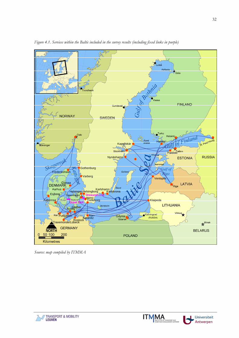
32

Figure 4.1. Services within the Baltic included in the survey results (including fixed links in purple)

Rostock

Trelleborg

Karlshamn

Ventspils

Nynäshamn

Klaipeda

Aarhus

Aabenraa

Hanko

Sassnitz

Helsingor HelsingborgOresund Link

GedserRodby

Puttgarten

Kapellskär

Paldiski

FrederikshavnGothenburg

Varberg

Grenaa

Great Belt

Travemünde/Lübeck

Esjberg

Gdynia

Karlskrona

Source: map compiled by ITMMA

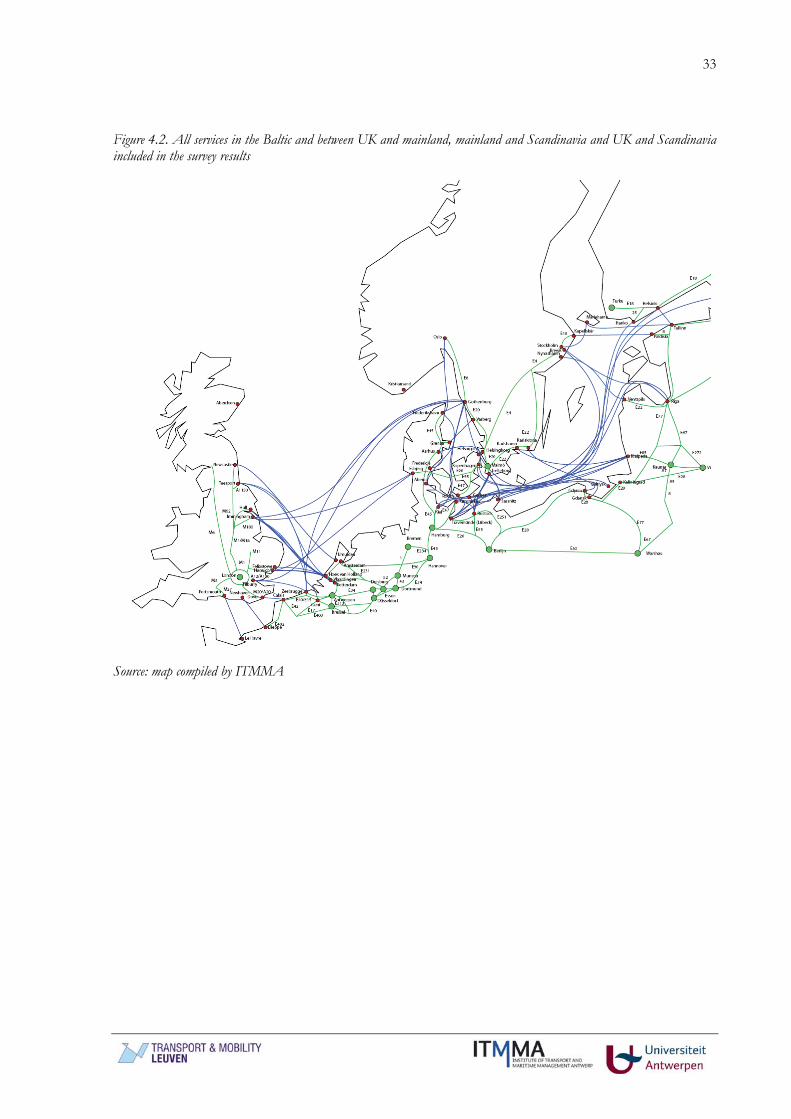
33

Figure 4.2. All services in the Baltic and between UK and mainland, mainland and Scandinavia and UK and Scandinavia included in the survey results

Source: map compiled by ITMMA

34

Table 4.2. Distribution of fuel types used by fleet for each of the distance classes (survey results- situation 2008)

Distance class

Total freight-unit km

Fuel consump

tion (tons)

0-125km 104,609,063 358,385 57.3% 19.7% 12.2% 0.0% 2.0% 8.8%125-400km 399,977,639 382,964 65.6% 10.1% 16.1% 3.5% 2.4% 2.3%400-750km 291,842,868 251,267 66.2% 5.5% 26.0% 0.6% 0.7% 1.0%>750km 542,842,212 323,036 90.5% 6.1% 0.0% 0.4% 0.7% 2.2%Total 1,339,271,783 1,315,652 69.6% 10.9% 13.0% 1.2% 1.6% 3.8%

MDO (0.2%-1.5%)

WRD (0.2%-1.5%)

MGO (≤0.1%)HFO ≤ 1.5% HFO ≤ 1% HFO ≤

0.5%

Table 4.3. Distribution of fuel types used by fleet for each of the sub-markets (survey results – situation 2008)

Distance class

Total freight-unit km

Fuel consump

tion (tons)

Rest intra-Baltic 347,481,353 429,737 61.0% 20.0% 13.2% 0.3% 2.0% 3.5%The Sound-Kattegat (intra) 159,152,948 288,834 35.0% 12.8% 39.3% 0.0% 3.6% 9.1%UK <-> LH-H range 440,512,926 421,010 92.2% 2.2% 0.0% 3.5% 0.4% 1.7%UK/LH-H range <-> Baltic 392,124,555 176,071 92.9% 6.0% 0.0% 0.0% 0.0% 1.0%Total 1,339,271,783 1,315,652 69.6% 10.9% 13.0% 1.2% 1.6% 3.8%

WRD (0.2%-1.5%)

MGO (≤0.1%)

HFO ≤ 1.5% HFO ≤ 1% HFO ≤

0.5%

MDO (0.2%-1.5%)

The distribution of the fuel types used is presented in tables 4.2 and 4.3. The survey results show that of the 1.32 million tons of fuel consumed by all vessels on the 64 services, nearly 70% is HFO with a maximum sulphur level of 1.5% (as minimally required by the current SECA regulations). Table 4.1 reveals that the share of HFO (1.5%) increases with distance and is particularly being used in services operating outside the Baltic. The use of MGO (0.1%) is the highest on the shorter routes, though even then the share remains below 9%. MDO and WRD are not commonly used (mainly to power auxiliary engines). Ships deployed on liner services within the Sound/Kattegat region are strongly relying on HFO with a low sulphur content of 0.5%. The use of this type of fuel grade is not common in other navigation areas. As MGO is hardly used at this moment, a shift to MGO would confront shipping lines with considerable fuel cost increases. Earlier sections in this report pointed to a cost increase per ton of bunker fuel of between 70 and 90% when moving from HFO (1.5%) to MGO (0.1%). At a price of USD 500 per ton of MGO this would imply an additional cost per ton of USD 205 to 235. All 64 services in the survey jointly consumed 915,000 tons of HFO (1.5%). The associated total cost of shifting this fuel mass to MGO (at the base scenario of USD 500 per ton) would equal to a staggering amount of between USD 190 and 220 million or 130 à 150 million euro (exchange rate of July 2009). For the high scenario (USD 1000 per ton) the total fuel cost increases would reach 260 à 300 million euro. The above figures exclude the price increases associated with the shift from other fuel types (i.e. HFO 1% and 0.5, MDO and WRD) to MGO. The figures relate to only 64 services operational in the ECAs.

35

Table 4.4. Expected impact of use of MGO in ECAs on the freight rates and the freight volumes – survey results per distance class

Distance class

Average distance

(one-way) in km

Number of lines

in survey


Increase in freight

rate

MGO: USD 200 per tonLoss of volume


Increase in freight

rate


MGO: USD 1000


rate

MGO: USD 1000

per tonLoss of volume

0-125km 65.1 16 7.3% 5.3% 15.3% 16.0% 30.5% 33.6%125-400km 269.2 21 6.3% 5.9% 15.6% 16.6% 33.9% 43.3%400-750km 518.5 13 3.1% 3.0% 20.6% 21.0% 56.0% 50.0%>750km 1007.4 14 3.2% -4.8% 20.7% 1.1% 57.8% 30.6%Total 430.3 64 5.1% 3.0% 17.7% 14.5% 42.7% 40.1%

PRICE FOR MGO USD/mt

Table 4.5. Expected impact of use of MGO in ECAs on the freight rates and the freight volumes – survey results per sub-market

Region

Average distance

(one-way) in km

Number of lines

in survey


Increase in freight

rate



Increase in freight

rate


MGO: USD 1000


rate

MGO: USD 1000

per tonLoss of volume

Rest intra-Baltic 588.9 21 -0.1% -2.8% 19.3% 11.3% 51.2% 52.1%The Sound-Kattegat (intra) 157.7 18 7.0% 4.2% 13.8% 14.7% 32.9% 37.7%UK <-> LH-H range 289.1 17 6.1% 8.5% 16.3% 21.9% 35.0% 49.1%UK/LH-H range <-> Baltic 927.4 8 12.8% - (*) 24.9% - (*) 58.6% - (*)Total 430.3 64 5.1% 3.0% 17.7% 14.5% 42.7% 40.1%

PRICE FOR MGO USD/mt

(*) no. of respondents too small for representative picture Tables 4.4 and 4.5 show the results per fuel price scenario for the questions ‘How would the use of MGO impact freight rates in three price scenarios?’ and ‘Can you estimate how much volume you would lose due to the assumed increases in freight rates?’. For the scenario of an MGO price of USD 500 per ton (the low scenario in the previous sections of this report), the respondents expect freight rate increases in the order of 15 to 25% with an overall average of nearly 18%. Rate increases are expected to be the highest on the longer routes. The corresponding volume losses are expected to reach 14.5%. The routes covering medium-range distances (400-750km) are likely to be hit the strongest with expected volume losses of 21% on average. The long-distance routes seem to be less affected. This might be explained by the limited modal shift potential from short sea to road (see discussion in the comparative cost analysis later in this report). For the high scenario (USD 1000 per ton), the expected impacts are considerable: a freight rate increase of up to 60% and anticipated volume losses of more than 50%. The medium-distance routes would be worst hit. When the MGO price would be as low as USD 200 per ton, the expected effects are quite marginal. However, the chance this scenario will materialize in the medium and longer term is very low.

36

In summary, the stated preference method deployed in this section demonstrates respondents expect that the use of MGO will lead to significant increases in freight rates and a decrease in freight volumes. It is interesting to compare the survey results with the results on freight rate increases presented in the previous section (see table 4.6). The survey results are in line with the simulation outcomes for the base and low scenarios. The stated-preference technique illustrates that the respondents of the ECSA survey have a slightly more pessimistic view on the implications of the high scenario for MGO prices compared to what came out of the simulation exercise. It must be stressed once again that the figures presented are averages and that quite substantial differences might exist among the different liner services. Table 4.6. Estimated increase in freight rates of short sea services following the use of MGO – comparison between average results of the ECSA survey and average results of the simulation exercise

Distance class

Average distance

(one-way) in km

Number of lines


Increase in freight

rate


Increase in freight

rate


Increase in freight

rate

MGO: USD 1000


rate

ECSA survey 430.3 64 5.14% 17.7% - 42.7%

Simulation - 18.5knots 721.7 16 - 11.5% 15.9% 19.7%

Simulation - fast ship 1,111 1 - 26.3% 34.0% 39.6% Source: compilation of tables 3.7, 4.4 and 4.5

4.4. Comparative cost/price analysis of the truck/short sea option versus the ‘truck only’ option

This section introduces a detailed comparative cost analysis to assess modal competition between the short sea/truck option and the ‘truck only’ option on 30 origin-destination routes linked to the ECAs. In a first step, cost functions for short sea/ropax vessels and trucks will be developed. In a second step, these cost functions will be applied to a set of origin-destinations relations. The aim is to identify to what extent the low sulphur fuel requirements will affect the modal split on each of the O-D routes. Based on the aggregated results, a more comprehensive picture can be drawn on expected modal shifts.

4.4.1. Cost functions for short sea vessels The cost per km incurred by a truck/trailer combination (equivalent to a vessel slot of 17 lane meters capacity) when using a short sea service is presented in figures 4.3. The functions were compiled on the basis of the base data deployed in the simulation exercise. The freight rate data and operational characteristics of the 17 roro/ropax services in the sample formed the basis for the estimation of a lower and upper limit to the unit cost per km of sailing distance. By doing so, four curves for each scenario could be drawn: upper and lower curves for HFO (1.5%) and upper and lower curves for MGO (0.1%). We are aware that many of the roro/ropax services transport unmanned cargo trailers (so only the trailer without truck and driver), but this fact in principle does not affect the results. The rates per km for shorter distances are much higher since fixed costs (such as port dues) have a large impact on the cost structure on short distances. The effect of such fixed costs flattens out when trip distances become longer.

37

Figure 4.3. Roro/ropax services: freight rate in euro per truck shipped per km sailing distance (for different scenarios)

0123456789

1011121314151617181920

25 100

175

250

325

400

475

550

625

700

775

850

925

1000

1075

1150

Frei

ght r

ate

in e

uro

per t

ruck

(17

lane

met

res)

per

km

Voyage sailing distance in km

MGO max

HFO max

MGO min

HFO min

HIGH SCENARIOMGO: USD 1000 per ton

0123456789

101112131415161718

25 100

175

250

325

400

475

550

625

700

775

850

925

1000

1075

1150

Frei

ght r

ate

in e

uro

per

truc

k (1

7 la

ne m

etre

s) p

er

km


MGO max

HFO max

MGO min

HFO min

BASE SCENARIOMGO: USD 750 per ton

0123456789

10111213141516

25 100

175

250

325

400

475

550

625

700

775

850

925

1000

1075

1150

Frei

ght r

ate

in e

uro

per t

ruck

(17

lane

met

res)

per

km


MGO max

HFO max

MGO min

HFO min

LOW SCENARIOMGO: USD 500 per ton

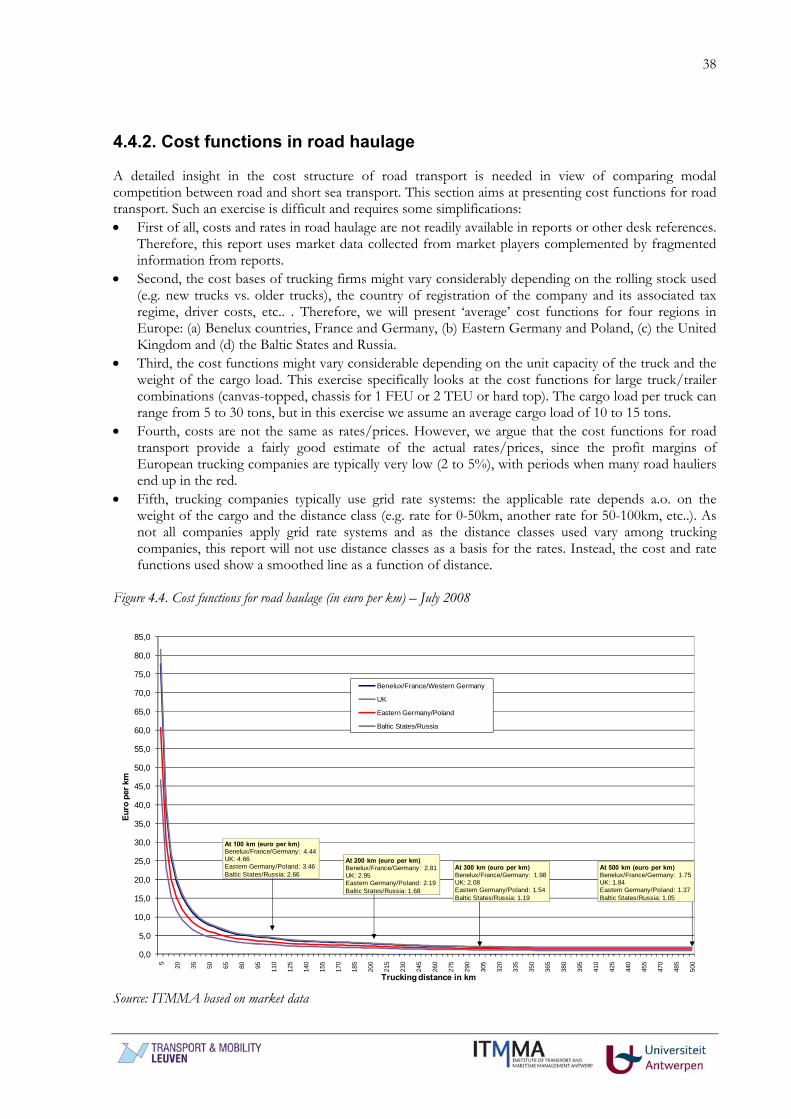
38

4.4.2. Cost functions in road haulage A detailed insight in the cost structure of road transport is needed in view of comparing modal competition between road and short sea transport. This section aims at presenting cost functions for road transport. Such an exercise is difficult and requires some simplifications: • First of all, costs and rates in road haulage are not readily available in reports or other desk references.

Therefore, this report uses market data collected from market players complemented by fragmented information from reports.

• Second, the cost bases of trucking firms might vary considerably depending on the rolling stock used (e.g. new trucks vs. older trucks), the country of registration of the company and its associated tax regime, driver costs, etc.. . Therefore, we will present ‘average’ cost functions for four regions in Europe: (a) Benelux countries, France and Germany, (b) Eastern Germany and Poland, (c) the United Kingdom and (d) the Baltic States and Russia.

• Third, the cost functions might vary considerable depending on the unit capacity of the truck and the weight of the cargo load. This exercise specifically looks at the cost functions for large truck/trailer combinations (canvas-topped, chassis for 1 FEU or 2 TEU or hard top). The cargo load per truck can range from 5 to 30 tons, but in this exercise we assume an average cargo load of 10 to 15 tons.

• Fourth, costs are not the same as rates/prices. However, we argue that the cost functions for road transport provide a fairly good estimate of the actual rates/prices, since the profit margins of European trucking companies are typically very low (2 to 5%), with periods when many road hauliers end up in the red.

• Fifth, trucking companies typically use grid rate systems: the applicable rate depends a.o. on the weight of the cargo and the distance class (e.g. rate for 0-50km, another rate for 50-100km, etc..). As not all companies apply grid rate systems and as the distance classes used vary among trucking companies, this report will not use distance classes as a basis for the rates. Instead, the cost and rate functions used show a smoothed line as a function of distance.

Figure 4.4. Cost functions for road haulage (in euro per km) – July 2008

0,0

5,0

10,0

15,0

20,0

25,0

30,0

35,0

40,0

45,0

50,0

55,0

60,0

65,0

70,0

75,0

80,0

85,0

5 20 35 50 65 80 95 110

125

140

155

170

185

200

215

230

245

260

275

290

305

320

335

350

365

380

395

410

425

440

455

470

485

500

Euro

per

km

Trucking distance in km

Benelux/France/Western Germany

UK

Eastern Germany/Poland

Baltic States/Russia

At 300 km (euro per km)Benelux/France/Germany: 1.98UK: 2.08Eastern Germany/Poland: 1.54Baltic States/Russia: 1.19




Source: ITMMA based on market data

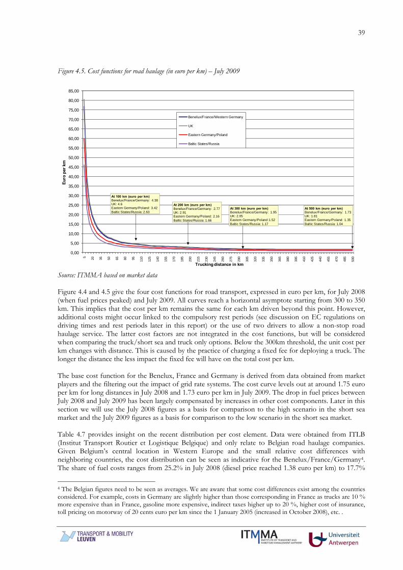
39

Figure 4.5. Cost functions for road haulage (in euro per km) – July 2009

0,00

5,00

10,00

15,00

20,00

25,00

30,00

35,00

40,00

45,00

50,00

55,00

60,00

65,00

70,00

75,00

80,00

85,00

5 20 35 50 65 80 95 110

125

140

155

170

185

200

215

230

245

260

275

290

305

320

335

350

365

380

395

410

425

440

455

470

485

500

Euro

per

km

Trucking distance in km

Benelux/France/Western Germany

UK

Eastern Germany/Poland

Baltic States/Russia

At 300 km (euro per km)Benelux/France/Germany: 1.95UK: 2.05Eastern Germany/Poland:1.52Baltic States/Russia: 1.17




Source: ITMMA based on market data Figure 4.4 and 4.5 give the four cost functions for road transport, expressed in euro per km, for July 2008 (when fuel prices peaked) and July 2009. All curves reach a horizontal asymptote starting from 300 to 350 km. This implies that the cost per km remains the same for each km driven beyond this point. However, additional costs might occur linked to the compulsory rest periods (see discussion on EC regulations on driving times and rest periods later in this report) or the use of two drivers to allow a non-stop road haulage service. The latter cost factors are not integrated in the cost functions, but will be considered when comparing the truck/short sea and truck only options. Below the 300km threshold, the unit cost per km changes with distance. This is caused by the practice of charging a fixed fee for deploying a truck. The longer the distance the less impact the fixed fee will have on the total cost per km. The base cost function for the Benelux, France and Germany is derived from data obtained from market players and the filtering out the impact of grid rate systems. The cost curve levels out at around 1.75 euro per km for long distances in July 2008 and 1.73 euro per km in July 2009. The drop in fuel prices between July 2008 and July 2009 has been largely compensated by increases in other cost components. Later in this section we will use the July 2008 figures as a basis for comparison to the high scenario in the short sea market and the July 2009 figures as a basis for comparison to the low scenario in the short sea market. Table 4.7 provides insight on the recent distribution per cost element. Data were obtained from ITLB (Institut Transport Routier et Logistique Belgique) and only relate to Belgian road haulage companies. Given Belgium’s central location in Western Europe and the small relative cost differences with neighboring countries, the cost distribution can be seen as indicative for the Benelux/France/Germany4. The share of fuel costs ranges from 25.2% in July 2008 (diesel price reached 1.38 euro per km) to 17.7%

4 The Belgian figures need to be seen as averages. We are aware that some cost differences exist among the countries considered. For example, costs in Germany are slightly higher than those corresponding in France as trucks are 10 % more expensive than in France, gasoline more expensive, indirect taxes higher up to 20 %, higher cost of insurance, toll pricing on motorway of 20 cents euro per km since the 1 January 2005 (increased in October 2008), etc. .

40

in January 2009 (diesel price of 0.99 euro per liter). Other significant cost components include driver costs (typically about one third of total costs) and amortization. Table 4.7. Overview of shares of cost components in Belgian road haulage companies (international transport only) July 2008 - diesel price at 1.38 per liter (including VAT)

Belgium-Germany Belgium-France Belgium-Italy Belgium-Spain AverageFuel 25.04% 24.99% 23.81% 26.66% 25.20%Tyres 2.70% 2.70% 2.58% 2.88% 2.72%Maintenance/revision 3.39% 3.38% 3.24% 3.61% 3.42%Amortization vehicle 11.54% 11.32% 9.46% 10.56% 10.47%Driver costs 32.10% 32.08% 27.16% 30.52% 29.91%Insurance vehicle 4.11% 4.11% 3.37% 3.76% 3.74%Insurance CMR/exploitation 0.72% 0.71% 0.59% 0.65% 0.65%Other direct vehicle costs 1.38% 1.37% 1.13% 1.26% 1.25%Capital costs (finance) 4.25% 4.19% 3.66% 3.94% 3.94%General costs 9.76% 9.58% 7.87% 8.77% 8.76%Specific trip costs 5.01% 5.57% 17.13% 7.39% 9.94%Total 100.00% 100.00% 100.00% 100.00% 100.00%January 2009 - diesel price at 0.99 per liter (including VAT)

Belgium-Germany Belgium-France Belgium-Italy Belgium-Spain AverageFuel 17.22% 17.67% 16.63% 18.99% 17.72%Tyres 2.90% 2.97% 2.84% 3.19% 3.00%Maintenance/revision 3.65% 3.74% 3.57% 4.02% 3.77%Amortization vehicle 12.19% 12.23% 10.19% 11.47% 11.29%Driver costs 34.35% 35.30% 29.77% 33.73% 32.78%Insurance vehicle 4.33% 4.44% 3.63% 4.09% 4.03%Insurance CMR/exploitation 0.76% 0.77% 0.63% 0.71% 0.70%Other direct vehicle costs 1.45% 1.49% 1.22% 1.37% 1.35%Capital costs (finance) 4.43% 4.44% 3.85% 4.18% 4.16%General costs 10.43% 10.53% 8.62% 9.70% 9.59%Specific trip costs 8.29% 6.42% 19.05% 8.55% 11.61%Total 100.00% 100.00% 100.00% 100.00% 100.00%July 2009 - diesel price at 1.05 per liter (including VAT)

Belgium-Germany Belgium-France Belgium-Italy Belgium-Spain AverageFuel 19.09% 19.54% 18.64% 20.25% 19.42%Tyres 2.83% 2.90% 2.76% 3.14% 2.93%Maintenance/revision 3.65% 3.75% 3.57% 4.05% 3.78%Amortization vehicle 11.89% 11.92% 9.93% 11.26% 11.03%Driver costs 33.55% 34.47% 29.05% 33.20% 32.09%Insurance vehicle 4.22% 4.33% 3.54% 4.01% 3.94%Insurance CMR/exploitation 0.74% 0.76% 0.62% 0.70% 0.69%Other direct vehicle costs 1.41% 1.45% 1.18% 1.34% 1.32%Capital costs (finance) 4.21% 4.21% 3.65% 3.99% 3.95%General costs 10.33% 10.43% 8.53% 9.67% 9.52%Specific trip costs 8.08% 6.24% 18.53% 8.39% 11.33%Total 100.00% 100.00% 100.00% 100.00% 100.00% Source: based on ITLB – monthly bulletins The base cost function for Eastern Germany and Poland is estimated using Polish drivers. The average cost per km for Polish trucking companies is significantly lower compared to companies from the other two regions considered. The cost difference is estimated at 20.2% in July 2008 and 21.3% in July 2009 in favour of the Polish companies. The cost curve for Poland levels out at around 1.37 euro per km (compared to 1.75 euro per km for the Benelux/France/Germany) for long distances in July 2008 and 1.35 euro per km in July 2009. The observed cost difference is not the result of fuel costs (diesel prices in Poland are very similar to the prices applicable in the Benelux/France/Germany), but is mainly caused by the gap in driver costs. Guihéry (2008:7) reports that the wages associated with one driving hour amount to 28.4 euro for France, 28.8 euro for the Netherlands, 25.9 euro for the western part of Germany, 15.4 euro for the eastern part of Germany5 and only 10 euro for Poland. The gap is not only the result of the

5 Even within one country, significant wage differences can occur. For example, German wages are ruled by a labor agreement negotiated at the Länder level which implies disparities between East and West Länder. ‘Low cost’ transport companies are mainly situated in East Germany facing direct competition from East European companies.

41

absolute wage differences. It is also associated with the weekly working time and the ratio between driving time and working time. In our analysis, the unit cost per km of Polish and East-German trucks is assumed to be 22% lower than for West German/Dutch trucking companies. Latvian, Estonian and Russian drivers dominate the market to and from the Baltic States. While exact figures are not available, the cost base of these trucking companies is said to be even much lower than the Polish case. When checking with Latvian forwarders and trucking companies, it was stated that the new wages per month for Latvian truck drivers would amount to 400 à 600 euro per month, compared to 800-900 euro for Polish drivers. Furthermore, the availability of cheap Russian diesel has a large impact on the cost base for these trucking companies. It is common practice to import Russian diesel in fuel tanks installed on old trucks and to fill the tanks of modern trucks once the Latvian/Russian border has been crossed. Russian diesel prices are as low as 0.38 à 0.40 euro per liter including tax. Because of these factors, it is not exceptional to see Baltic and Russian trucking companies operate at a cost per km up to a level of 1 euro per km or almost half of the operating costs of German or Dutch companies. Given these practices, the simulation model uses much lower trucking rates on routes to the Baltic States and Eastern Europe compared to routes in Western Europe. In our analysis, the unit cost per km of Baltic and Russian trucks is assumed to be 40% lower than for West German/Dutch trucking companies. The road haulage costs for UK companies are the highest of the three cost curves considered. Trucking companies based in the southeastern part of the United Kingdom on average face a 5% higher cost per km then their counterparts across the English Channel, at least when operational in the UK. This is mainly caused by the higher diesel prices in the United Kingdom (see figure 3.2 earlier in this report). Deliveries to London suffer from relatively high costs stemming mainly from motorway routing via the congested M25 and urban delays on the M25. Road transport, in, around and near to London is expensive with rates 15% to 40% higher than over less congested routes. We generalize trucking costs for UK companies at 1.84 euro per km for July 2008 and 1.81 euro per km for July 2009. In our analysis, the unit cost per km of UK trucks is assumed to be 5% higher than for West German/Dutch trucking companies. The cost curves presented in this section serve as a basis for the comparative analysis between the short sea/truck option and the ‘truck only’ option further in this study. In order to make this comparison realistic we developed a nationality distribution of trucks operational on each of the four main short sea-markets in North-Europe. On the links between West Europe and Scandinavia we primarily find Dutch and German truck drivers. Road haulage across the English channel is dominated by West-European firms. Baltic and Russian drivers are dominant on the connections between West Europe and the Baltic States (table 4.8). Table 4.8. Distribution of trucks for different routes

Germany/Denmark to Sweden English Channel West Europe-Baltic States West Europe-ScandinaviaBenelux/France/Western Germany 75% 50% 20% 70%UK 0% 40% 0% 0%Eastern Germany/Poland 20% 5% 25% 15%Baltic States/Russia 5% 5% 55% 15% Source: based on market information

East German drivers can then be paid 30% less than in the West when labour agreements are applied which is not the case every time.

42

4.4.3. Comparative cost analysis on origin-destination pairs In this section we develop a comparative cost analysis for a set of 30 origin-destination pairs centered around four short sea routes (see table 4.9 and figures 4.6 to 4.9): • Germany/Denmark to Sweden • English Channel • West Europe to Baltic States • West Europe to Scandinavia (Sweden/Norway) Different short sea service routes can be considered per origin-destination pair. All these short sea solutions face potential competition from a ‘truck only’ option (for Dover-Calais in combination with the Channel Tunnel). The Baltic States can be reached from Western Europe by following the highways and main roads connecting Germany, Poland and the eastern Baltic. The cost model used in this section takes into account the following cost components Unit rates per kilometer The unit rates per km are based on the cost functions for trucks and short sea introduced in earlier sections and take into account the nationality distribution of trucks as presented in table 4.8. Distances The road distances were determined using a route planner, while the sailing distances for short sea vessels are based on the maritime distance calculator available at www.dataloy.com . They are presented in table 4.9. Transport time The transport time is part of this cost exercise, as we have to take into account minimum rest periods and maximum driving times for the road haulage industry. Regulation (EC) 561/2006 of the European Commission provides a common set of EU rules for maximum daily and fortnightly driving times as well as daily and weekly minimum rest periods for all drivers of road haulage and passenger transport vehicles, subject to specified exceptions and derogations. The regulation is quite complex6. The cost model includes minimum rest periods and maximum driving times in the following manner. First of all, every 4,5 hours driving time there is a compulsory rest period of 45min. Secondly, the driver can only drive 9 hours per day and should then have a rest period as prescribed by the EC Regulation. In practice, the cost model assumes one driver respecting the specifications on rest periods and driving times. This assumption does not always correspond with daily practices in the trucking sector since long distance road transport often involves two drivers (with implications on the cost per km). The additional costs of rest periods are integrated in the cost model by combining driving time with compulsory rest periods. For trucking a distinction is made between highways and non-highways. For the highways, the average driving speed is set at 90 km/h, for other roads 75 km/h. The commercial speed of roro/ropax vessels in this analysis amounts to 18.5 knots (34.3 km/h).

6 The main elements in the regulation can be summarized as follows. The daily driving period can not exceed 9 hours, with an exemption of twice a week when it may be 10 hours. There can be six driving periods per week. The total weekly driving time may not exceed 56 hours and the total fortnightly driving time may not exceed 90 hours. The daily rest period shall be at least 11 hours, with an exception of going down to 9 hours three times a week. There is provision for a split rest of 3 hours followed by 9 hour rests to make a total of 12 hours rest per day. Weekly rest is 45 continuous hours, which can be reduced to 24 hours. Compensation arrangements apply for reduced weekly rest periods. Breaks of at least 45 minutes (separable into 15 minutes followed by 30 minutes) should be taken after 4 ½ hours at the latest.

43

Table 4.9. Origin-destination relations considered in the comparative cost analysis DISTANCES Alternative 1 (truck only) Alternative 2 (truck/shortsea) Alternative 3 (truck/shortsea) Alternative 4 (truck/shortsea)

Truck total Rail Truck (pre) Shortsea Truck (post) Truck total Truck (pre) Shortsea Truck (post) Truck total Truck (pre) Shortsea Truck (post) Truck total(km) (km) (km) (km) (km) (km) (km) (km) (km) (km) (km) (km) (km) (km)

Germany/Denmark to Sweden via Travemünde-Trelleborg via Putgarten-Rödby and Oresund via Putgarten-Rödby and Helsingör-Helsingborg1.1. Dortmund - Göteborg 1133 (F+O) 0 421 224 303 724 681 20 461 (O) 1142 681 26 411 10921.2. Dortmund - Stockholm 1499 (F+O) 0 421 224 646 1067 681 20 805 (O) 1486 681 26 755 1436

(*) (**)English Channel via Chunnel via Calais-Dover via Rotterdam-Harwich via Rotterdam-Hull2.1. Rotterdam - Tilbury 428 40 312 43 116 428 30 204 109 139 - - - -2.2. Rotterdam - London 452 40 312 43 140 452 30 204 128 158 - - - -2.3. Rotterdam - Portsmouth 538 40 312 43 226 538 30 204 263 293 - - - -2.4. Düsseldorf - Tilbury 515 40 401 43 116 517 260 204 109 369 - - - -2.5. Düsseldorf - London 540 40 401 43 140 541 260 204 128 388 - - - -2.6. Düsseldorf - Portsmouth 626 40 401 43 226 627 260 204 263 523 - - - -2.7. Brussels - Tilbury 315 40 201 43 116 317 179 204 109 288 - - - -2.8. Brussels - London 340 40 201 43 140 341 179 204 128 307 - - - -2.9. Brussels - Portsmouth 426 40 201 43 226 427 179 204 263 442 - - - -2.10. Dortmund - Tilbury 557 40 442 43 116 558 279 204 109 388 - - - -2.11. Dortmund - London 582 40 442 43 140 582 279 204 128 407 - - - -2.12. Dortmund - Portsmouth 668 40 442 43 226 668 279 204 263 542 - - - -2.13. Rotterdam - Manchester 787 40 312 43 475 787 30 204 400 430 30 335 154 1842.14. Düsseldorf - Manchester 876 40 401 43 475 876 260 204 400 660 260 335 154 4142.15. Brussels - Manchester 676 40 201 43 475 676 179 204 400 579 179 335 154 3332.16. Dortmund - Manchester 917 40 442 43 475 917 279 204 400 679 279 335 154 433

West Europe-Baltic States via Lübeck-Riga via Kappelskär-Paldiski Via Karlshamn-Klaipeda3.1. Dieppe - Tallinn 2458 0 1006 1011 309 1315 - - - - - - - -3.2. Dieppe - Kaunas 1845 0 1006 1011 264 1270 - - - - - - - -3.3. Antwerpen - Tallinn 2236 0 636 1011 309 945 - - - - - - - -3.4. Antwerpen - Kaunas 1669 0 636 1011 264 900 - - - - - - - -3.5. Amsterdam - Tallinn 2171 0 642 1011 309 951 - - - - - - - -3.6. Amsterdam - Kaunas 1604 0 642 1011 264 906 - - - - - - - -3.7. Hamburg - Tallinn 1830 0 67 1011 309 376 - - - - - - - -3.8. Hamburg - Kaunas 1263 0 67 1011 264 331 - - - - - - - -3.9. Esbjerg - Tallinn 2128 0 374 1011 309 683 1030 (F+O) 296 51 1081 - - - -3.10. Esbjerg - Kaunas 1561 0 374 1011 264 638 - - - - 483 (F+O) 413 215 698

West Europe-Scandinavia via Ghent-Göteborg via Travemünde-Trelleborg via Putgarten-Rödby4.1. Rotterdam - Oslo 1554 (F+O) 0 157 1083 294 451 577 224 597 1174 835 20 756 (O) 15914.2. Rotterdam - Stockholm 1606 (F+O) 0 157 1083 469 626 577 224 646 1223 835 20 805 (O) 1640

Notes: (*) 20 km for Putgarten-Rödby and 6km for Helsingör-Helsingborg (**) Of which 198km between Rödby and Helsingör (O) = via Öresund-link (F+O) = via Great Belt and Öresund-link

44

Figure 4.6. Geographical representation of routes between Germany/Denmark to Sweden

Source: ITMMA Figure 4.7. Geographical representation of routes on the English Channel

Source: ITMMA

45

Figure 4.8. Geographical representation of routes between West Europe and the Baltic States

Source: ITMMA Figure 4.9. Geographical representation of routes between West Europe and Scandinavia

Source: ITMMA

46

Fees/tolls for fixed links Trucks might be confronted with additional costs when using fixed links between land masses separated by water. On the English Channel, ferries face stiff competition from the Eurotunnel, at least for manned truck/trailer combinations. The cross Channel market for the transport of unmanned units (trailers only) is fully in the hands of ferry operators. In 2008, Eurotunnel has transported 1,254,282 trucks on its Shuttles between Folkestone and Calais, i.e. the equivalent of 14.2 million tons of goods. The Shuttles dedicated to trucks can transport up to 30 trucks in semi-enclosed wagons. The drivers do not remain in their vehicles, but travel in an amenity car, which offers catering facilities. Trucks cross the Straits in 90 minutes at the most, from the M20 motorway in the UK to the A16 motorway in France, including time for boarder controls, loading, crossing and unloading. Truck shuttles leave every 10, 12 or 15 minutes depending on traffic levels, and drivers do not need to book ahead. The flexible timetables are adjusted to traffic levels every day. The tariff for a truck of 13-15m is about 300-350 euro excl. VAT (one-way, excluding discounts, online booking system www.eurotunnel.com ). Eurotunnel’s current strategy, introduced some 2 or 3 years ago to keep its payroll and energy costs to a minimum, is to run fewer freight shuttles than previously, but to run them full. They do this by offering very competitive rates to large hauliers, but under very restrictive terms – a very good price for pre-booked slots on nominated shuttles, but punitively high charges for spot bookings (or last minute changes). This strategy enables Eurotunnel to control its operating costs, but at the expense of offering low flexibility to its customers. The ferries, by contrast, offer flexibility (“turn up and go when you want”). The fixed links in Denmark (Great Belt Link and Oresund Link) make it possible for truck drivers to drive from the European mainland to Sweden and Norway. The use of these fixed links is not free of charge. Table 4.10 gives an overview of the toll for driving the Oresund fixed link (one way trip without discount) in Danish kroner (DKK), Swedish kronor (SEK) and euro for April 2009. The full price for a truck/trailer combination is 109 euro incl. VAT or 85.7 euro excl. VAT (one-way). Discounts apply to most of the trucking companies frequently using the connection (3.3% for 500-5,000 crossings and 6.4% for 5,000-10,000 crossings per year, see www.oresundsbron.com). In our cost analysis we use 85 euro as a base rate for trucks. There has been criticism of the tolls which are much higher than many consider reasonable for a bridge. However they are compatible with the ferry charges that were levied before the bridge was built and for the ferries still running between Helsingborg-Helsingør. For example, Scandlines charges 113 euro for a truck of 13m and 139 euro for a truck up to 19m (rates excluding VAT, Bunker Adjustment Factor – BAF and other surcharges that may apply) on the ferry link between Helsingborg and Helsingør (6 km distance). Special rates apply for transit traffic that uses the Helsingør – Helsingborg ferry as well as the Puttgarden – Rødby or Rostock – Gedser ferry link (both connect Germany to Denmark): 311 euro for a truck of 13m and 387 euro for a truck up to 19m. These are the official rates. In practice, the negotiated price for large customers for the combined ferry connection Helsingør – Helsingborg and Puttgarden – Rødby can be as low as 200 euro. Using our roro cost functions as presented in figure 4.3, the combined ferry connection amounts to 198 euro (min) to 403 euro (max) for the use of HFO in the high scenario and between 172 euro and 360 euro for the use of HFO in the low scenario. Another important fixed link is the Great Belt Fixed Link connecting the Danish towns of Korsør and Nyborg on the islands of Zealand (Sjælland) and Fyn (or Funen) respectively. It consists of a road suspension bridge and railway tunnel between Zealand and the islet Sprogø, as well as a box girder bridge between Sprogø and Funen. The link replaces the ferries which had been the primary means of crossing Great Belt for more than 100 years. The link was opened to road traffic in 1998. The link has produced considerable time savings for travel and transport between eastern and western Denmark. Previously, the average elapsed time involved in transfer by ferry across the Great Belt was approximately 90 minutes, including the waiting time at the harbours. The time was considerably higher during peak volume periods. After the opening of the Great Belt Link, the elapsed time has fallen to between 10 and 15 minutes. The 2009 toll fees for trucks (10-19m) amount to 142 euro incl. VAT (one-way, figures www.storebaelt.dk, excluding discounts) or 114 euro excl. VAT. In our analysis we use a market-based fee of 110 euro per transit. A combined use of the Oresund Link and the Great Belt Link thus costs about 195 euro (excl. VAT).

47

Table 4.10. Toll for driving the Oresund fixed link (one way trip without discount – including VAT)

Vehicle DKK SEK EuroMotorcycle 150 220 21Standard car 275 395 38Motorhome/car+caravan 550 790 75Minibus (6-9 metres) 550 790 75Bus (longer than 9 metres) 1145 1675 157Lorry/truck (9-20 metres) 795 1170 109Lorry/truck (over 20 metres) 1190 1755 163 Eurovignet for trucks For the integration of the Eurovignet in the analysis we follow the approach as suggested by Skema (2010). COM(2008) 436 final/2 proposed amendments to Directive 1999/62/EC on the charging of heavy goods vehicles for the use of certain infrastructures. The proposal was based on the “Handbook on estimation of external costs in the transport sector”, produced within the study “Internalisation Measures and Policies for All external Cost of Transport” (IMPACT). In this report the Commission proposed that road users should also be charged, on a per kilometre basis, for air pollution, noise pollution and congestion in addition to current infrastructural tolls. Skema (2010) calculated that this would imply an average environmental charge per vehicle-km of 0.053 euro for EURO IV trucks and 0.034 euro for EURO V and VI trucks. These kilometer charges for environmental impact (external costs) are part of a proposed amendment to the current Eurovignet Directive and as such have not yet been ratified. In their study, Skema (2010) assumed that these charges will be ratified by the European Parliament and fully implemented and enforced by 2015. We therefore assume that the proposed environmental tolls will be 100% implemented in their current form in 2015. We also follow the assumption that the current prescribed infrastructural tolls by 2015 will be 100% enforced compared to only 50% now. We assume that EURO VI trucks will be the norm by 2015. Given the above assumptions, the additional charge per vehicle-km for EURO VI trucks would amount to 0.0385 euro per vehicle-km, i.e. an environmental charge of 0.034 euro per vehicle-km and an additional infrastructure charge of 0.0045 euro per vehicle-km. The 100% infrastructural toll upper limit for a EURO VI truck is 0.009 euro per vehicle-km, but since we assume 50% of this amount is already charged today we stick to an additional infrastructure charge of 0.0045 euro per vehicle-km (see also Skema study). In our cost analysis we use an additional charge caused by the Eurovignet of 0.0385 euro per vehicle-km. A full application of the Eurovignet will thus lead to an increase in cost price per km for trucks. However, this cost increase is quite modest: the base cost per vehicle-km for West European trucking companies amounts to around 1.75 euro (see figures 4.4 and 4.5 earlier in this report). The additional charge of 0.0385 would bring this amount to about 1.79 euro per vehicle-km, an increase of about 2.2%. Moreover, it is expected that this cost increase might be compensated by: • A higher load factor on trucks (see impact of LKW Maut in Germany on load factors of trucks) • More efficient truck technology: an important point here is that the trucking industry has much more

flexibility to adapt to changing rules regarding emissions. Efficiency gains due to new technologies develop rather fast in the trucking industry, but need more implementation time in the shipping industry. One of the reasons is that trucks are amortized over a period of 3 to 4 years, while in shipping vessels have a much longer lifecycle.

• A partial compensation of the Eurovignet by a lowering by governments of the fixed costs of trucks (in particular the vehicle tax) and some of the variable costs (tax on diesel).

• A further influx of East-European drivers on the West-European markets.

48

The comparative cost analysis compares five prices for each of the 30 origin-destination relations: • The total price for the ‘truck only’ option (i.e. truck is the only transport mode used on the O-D

relation); • The total minimum price for the combined truck/short sea option with a roro/ropax vessel using

HFO (1.5%) as base fuel; • The total maximum price for the combined truck/short sea option with a roro/ropax vessel using

HFO (1.5%) as base fuel; • The total minimum price for the combined truck/short sea option with a roro/ropax vessel using

MGO (0.1%) as base fuel; • The total maximum price for the combined truck/short sea option with a roro/ropax vessel using

MGO (0.1%) as base fuel; The differences between the minimum and maximum price scenarios for the truck/short sea options are linked to the cost functions for roro/ropax vessels as depicted earlier in figure 4.3. The model output makes it possible to compare the ‘truck only’ option with one or more combined truck/short sea options for each of the scenarios regarding the evolution of the price of MGO and HFO. We limit the analysis to the high scenario and the low scenario. Moreover, the model output gives an indication of the impact of the use of MGO on the price for the combined truck/short sea option. The results for the 30 origin-destination relations are presented in the tables below. The results are route-specific. The main conclusions of the cost analysis can be divided in two groups.

First of all, we can draw conclusions regarding the expected total cost changes per origin-destination relation. The results are presented in table 4.11 (high scenario) and table 4.12 (low scenario). On origin-destination relations with an ultra-short or short maritime section (Calais-Dover, Putgarten-Rödby, Helsingör-Helsingborg and Travemünde-Trelleborg) the total price increase typically ranges between 1% and 8% for the high scenario and 0.5% and 4% for the low scenario. Differences between these routes are partly the result of detour distances for trucks and the existence of fees for using fixed links. The more important the short sea section is in the total transport distance, the more impact the use of MGO (0.1%) has on the total price for the truck/short sea option. For example, on the Rotterdam-Oslo route (no. 4.1) the price increase associated with the shift from HFO to MGO reaches about 11 to 12% in the high scenario when using the Ghent-Göteborg short sea link. When using shorter short sea links (alternatives 3 and 4) the price increase ranges between 1.1% and 3.4%. In other words, the use of MGO is expected to increase the transport prices particularly on the origin-destination relations with a medium or long short sea section. Such a price development might eventually trigger a shift from medium and long short sea routes to shorter short sea routes or a ‘truck only’ alternative without any short sea section. Secondly, we can draw conclusions regarding changes in the relative competitive position of the short sea/truck option versus the ‘truck only’ option when using MGO (0.1%) instead of HFO (1.5%) (per origin-destination relation). The results are presented in table 4.13 (high scenario) and table 4.14 (low scenario). Tables 4.15 and 4.16 summarize the main findings using average cost differences linked to a color scale. The results per trade relation are presented in the next paragraphs: 1. On the trade lane between Germany/Denmark and Sweden, the Travemünde-Trelleborg ferry

connection is competitive compared to the ‘truck only’ option. Trucks typically incur higher costs as a consequence of significant additional distances to be travelled and tolls linked to the use of the fixed links in Denmark (Great Belt and Oresund). For the shorter short sea routes (alternatives 3 and 4), the price difference between the combined truck/short sea solution and the ‘truck only’ option diminishes when using MGO instead of HFO up to a level where the ‘truck only’ option becomes more competitive. The observed price gap, though small, can trigger a modal shift from sea to road in the high scenario.

49

2. The cross channel short sea business for manned truck/trailer combinations is likely to be hit hard by the use of MGO. At present the rate setting of short sea services on the Calais-Dover link is still competitive compared to the Eurotunnel shuttle services: the position of the ferry links ranges between a cost advantage of 6 to a cost disadvantage of up to 22% on some links. However, the use of MGO makes the price difference on the O-D relations considered shifts in favour of the freight rail shuttles through the Channel Tunnel (see also average figures and color codes in table 4.15). The combined truck/short sea solution ends up having a price disadvantage of 32% (maximum) and 0% (minimum) compared to the truck/rail combination. These results suggest a modal shift from short sea services on the Calais-Dover link to rail services through the Channel Tunnel. The tunnel is estimated at 75% capacity prior to the fire and is at 50% capacity now. Eurotunnel is aggressively seeking to regain lost market share. The use of MGO (0.1%) will allow Eurotunnel to introduce extra freight shuttles but, unless it abandons its strict cost-control strategy, Eurotunnel would presumably do so only if it thought they would be full, not on the off-chance of picking up the odd extra lorry. In summary, the use of MGO could well imply a major traffic loss of manned truck/trailer combinations per vessel across the southern part of the English Channel with potentially negative implications on the ferry capacity for passenger transfers. The Rotterdam-Harwich short sea link shows the most competitive profile on all routes considered except for traffic flows to and from Manchester (price dominance of Rotterdam-Hull), but also here the use of MGO is expected to make its competitive position weaker: the average price advantage over the truck/rail option via the Channel Tunnel in the high scenario decreases from 13% to 8%. The narrowing of the price gap implies that the Rotterdam-Harwich short sea route moves towards a situation of increased competition with the truck/rail option. Such a development should raise great concern given longer truck distances on the already highly congested motorways in the southeast of the UK..

3. The transport connections between Western Europe and the Baltic States are expected to be heavily affected by the introduction of the new regulations on low sulphur requirements for vessels in the ECAs. While long-distance short sea transport succeeds in keeping a cost advantage over trucking on a number of O-D relations (see for example Hamburg-Tallinn), the ratio between the trucking price and the price for the truck/short sea combinations seriously deteriorates on most other routes. On the routes Dieppe-Kaunas and Amsterdam-Kaunas, short sea services are likely to completely lose their appeal to customers which implying major modal shifts away from the Lübeck-Riga short sea link. On the routes Hamburg-Kaunas and Antwerp-Kaunas, the price disadvantage for the long-distance short sea solution becomes too high to guarantee a high competitiveness vis-à-vis trucking. Alternative short sea routes 3 and 4 remain competitive for connecting Esjberg to the Baltic States, but also there the price difference shrinks when introducing MGO.

4. At present, the short sea connections between the Benelux/Western Germany and Scandinavia

(Sweden and Norway in particular) face rather limited competition from road haulage. The main competitor is the much shorter short sea link between Travemünde and Trelleborg (which involves much longer trucking distances). Nevertheless, the use of MGO is expected to narrow down the cost advantage of the long-distance short sea option to such an extent that some customers might start opting for trucking goods instead of using short sea services. More certain is that the use of MGO will trigger a shift from long-distance to short-distance short sea links. Hence, the Travemünde-Trelleborg route clearly overtakes the Ghent-Göteborg route to become the cheapest solution between Rotterdam and Stockholm, while the price gap also closes on the Rotterdam-Oslo link.

The results for the low scenario (table 4.14 and 4.16) are slightly more positive for short sea services than in the high scenario, but still the use of MGO (0.1%) is expected to generate shifts from sea to road given the observed changes in the ratios between the truck prices and the truck/short sea prices. The logistics industry is sensitive to price changes. The observed shifts in price differences incurred when introducing MGO (0.1%) as a base fuel in the ECAs would undoubtedly lead to changes in the modal split at the expense of short sea services. We also indicated that on some routes shifts from long-distance to

50

short-distance short sea routes are to be expected. Traffic losses for short sea services force short sea operators to reduce capacity, to downsize vessels deployed (leading to less economies of scale) and to limit frequency of their services. Lower frequencies and higher operational costs linked to smaller vessels further reduce the attractiveness/competiveness of the short sea option. If traffic losses reach a level no longer allowing the short sea operator to guarantee a minimum service frequency then a complete closure of the line is a probable outcome. In other words, even relatively small traffic losses (e.g. 10% to 20% less cargo) for existing short sea services can trigger a vicious cycle of capacity reduction and lower frequencies ultimately leading to a poorer position for short sea services and thus an unattractive market environment for investors. Vicious cycles characterized by the downsizing of short sea activities and the closures of lines can lead to an overall implosion of a short sea sub-market, leaving room to the ‘truck only’ option or short sea services on short or ultra-short distances to fill the gap in the market. In the next section, the influence of the new requirements of IMO on the total external costs will be examined for the same 30 origin-destination pairs. Table 4.11. Impact of the use of MGO on the total cost per routing alternative – expected price increases in % for transport between origin and destination (truck + short sea) - HIGH scenario

Alternative 2 (shortsea+truck) Alternative 3 (shortsea+truck) Alternative 4 (shortsea+truck)roro min roro max roro min roro max roro min roro max

Germany/Denmark to Sweden via Travemünde-Trelleborg via Putgarten-Rödby and Oresund via P-R and Helsingör-Helsingborg1.1. Dortmund - Göteborg 3.2% 4.8% 1.4% 2.4% 2.0% 3.2%1.2. Dortmund - Stockholm 2.3% 3.6% 1.1% 1.9% 1.6% 2.5%

English Channel via Calais-Dover via Rotterdam-Harwich via Rotterdam-Hull2.1. Rotterdam - Tilbury 5.0% 7.0% 6.9% 8.9% - -2.2. Rotterdam - London 4.8% 6.8% 6.5% 8.6% - -2.3. Rotterdam - Portsmouth 4.2% 6.1% 5.9% 8.0% - -2.4. Düsseldorf - Tilbury 4.3% 6.2% 5.5% 7.6% - -2.5. Düsseldorf - London 4.2% 6.1% 5.3% 7.4% - -2.6. Düsseldorf - Portsmouth 3.7% 5.5% 4.2% 6.1% - -2.7. Brussels - Tilbury 5.8% 7.9% 6.0% 8.0% - -2.8. Brussels - London 5.8% 7.8% 5.9% 7.9% - -2.9. Brussels - Portsmouth 5.0% 7.0% 4.8% 6.8% - -2.10. Dortmund - Tilbury 4.1% 5.9% 5.3% 7.4% - -2.11. Dortmund - London 3.9% 5.8% 5.1% 7.1% - -2.12. Dortmund - Portsmouth 3.5% 5.3% 4.1% 6.0% - -2.13. Rotterdam - Manchester 3.1% 4.7% 4.9% 6.9% 6.5% 8.6%2.14. Düsseldorf - Manchester 2.8% 4.3% 3.5% 5.2% 5.3% 7.4%2.15. Brussels - Manchester 3.5% 5.2% 3.9% 5.7% 6.0% 8.1%2.16. Dortmund - Manchester 2.7% 4.2% 3.4% 5.1% 5.2% 7.2%

West Europe-Baltic States via Lübeck-Riga via Kappelskär-Paldiski Via Karlshamn-Klaipeda3.1. Dieppe - Tallinn 6.3% 8.4% - - - -3.2. Dieppe - Kaunas 6.5% 8.6% - - - -3.3. Antwerpen - Tallinn 7.9% 9.9% - - - -3.4. Antwerpen - Kaunas 8.1% 10.1% - - - -3.5. Amsterdam - Tallinn 7.8% 9.8% - - - -3.6. Amsterdam - Kaunas 8.1% 10.1% - - - -3.7. Hamburg - Tallinn 12.5% 13.4% - - - -3.8. Hamburg - Kaunas 12.8% 13.7% - - - -3.9. Esbjerg - Tallinn 9.5% 11.3% 2.6% 4.0% - -3.10. Esbjerg - Kaunas 9.8% 11.5% - - 4.5% 6.5%

West Europe-Scandinavia via Ghent-Göteborg via Travemünde-Trelleborg via Putgarten-Rödby4.1. Rotterdam - Oslo 10.8% 12.3% 2.1% 3.4% 1.1% 1.8%4.2. Rotterdam - Stockholm 9.2% 11.0% 2.1% 3.3% 1.1% 1.8%

51

Table 4.12. Impact of the use of MGO on the total cost per routing alternative – expected price increases in % for transport between origin and destination (truck + short sea) - LOW scenario

Alternative 2 (shortsea+truck) Alternative 3 (shortsea+truck) Alternative 4 (shortsea+truck)roro min roro max roro min roro max roro min roro max

Germany/Denmark to Sweden via Travemünde-Trelleborg via Putgarten-Rödby and Oresund via P-R and Helsingör-Helsingborg1.1. Dortmund - Göteborg 1.7% 2.4% 0.8% 1.2% 1.1% 1.6%1.2. Dortmund - Stockholm 1.2% 1.8% 0.6% 0.9% 0.8% 1.3%

English Channel via Calais-Dover via Rotterdam-Harwich via Rotterdam-Hull2.1. Rotterdam - Tilbury 2.7% 3.6% 3.7% 4.7% - -2.2. Rotterdam - London 2.6% 3.5% 3.6% 4.5% - -2.3. Rotterdam - Portsmouth 2.3% 3.1% 3.2% 4.2% - -2.4. Düsseldorf - Tilbury 2.3% 3.2% 3.0% 3.9% - -2.5. Düsseldorf - London 2.2% 3.1% 2.9% 3.8% - -2.6. Düsseldorf - Portsmouth 2.0% 2.8% 2.3% 3.1% - -2.7. Brussels - Tilbury 3.2% 4.1% 3.2% 4.2% - -2.8. Brussels - London 3.1% 4.1% 3.1% 4.1% - -2.9. Brussels - Portsmouth 2.7% 3.6% 2.6% 3.5% - -2.10. Dortmund - Tilbury 2.2% 3.0% 2.9% 3.8% - -2.11. Dortmund - London 2.1% 3.0% 2.8% 3.7% - -2.12. Dortmund - Portsmouth 1.9% 2.7% 2.2% 3.1% - -2.13. Rotterdam - Manchester 1.6% 2.4% 2.7% 3.6% 3.5% 4.5%2.14. Düsseldorf - Manchester 1.5% 2.2% 1.9% 2.7% 2.9% 3.8%2.15. Brussels - Manchester 1.9% 2.7% 2.1% 2.9% 3.3% 4.2%2.16. Dortmund - Manchester 1.4% 2.1% 1.8% 2.6% 2.8% 3.7%

West Europe-Baltic States via Lübeck-Riga via Kappelskär-Paldiski Via Karlshamn-Klaipeda3.1. Dieppe - Tallinn 3.5% 4.4% - - - -3.2. Dieppe - Kaunas 3.6% 4.5% - - - -3.3. Antwerpen - Tallinn 4.3% 5.2% - - - -3.4. Antwerpen - Kaunas 4.5% 5.3% - - - -3.5. Amsterdam - Tallinn 4.3% 5.2% - - - -3.6. Amsterdam - Kaunas 4.5% 5.3% - - - -3.7. Hamburg - Tallinn 7.1% 7.2% - - - -3.8. Hamburg - Kaunas 7.3% 7.4% - - - -3.9. Esbjerg - Tallinn 5.3% 6.0% 1.4% 2.0% - -3.10. Esbjerg - Kaunas 5.5% 6.1% - - 2.4% 3.3%

West Europe-Scandinavia via Ghent-Göteborg via Travemünde-Trelleborg via Putgarten-Rödby4.1. Rotterdam - Oslo 6.1% 6.6% 1.1% 1.7% 0.6% 0.9%4.2. Rotterdam - Stockholm 5.1% 5.8% 1.1% 1.7% 0.6% 0.9%

52

Table 4.13. Results of the comparative cost analysis – high scenario (HFO = 386 euro/ton , MGO = 695 euro/ton), cost for ‘truck only’ option (alternative 1) is index 100 Cost for 'truck only' option Alternative 2 (shortsea+truck) Alternative 3 (shortsea+truck) Alternative 4 (shortsea+truck)(alternative 1) = 100 Use of HFO (1.5%) Use of MGO (0.1%) Use of HFO (1.5%) Use of MGO (0.1%) Use of HFO (1.5%) Use of MGO (0.1%)

roro min roro max roro min roro max roro min roro max roro min roro max roro min roro max roro min roro maxGermany/Denmark to Sweden via Travemünde-Trelleborg via Putgarten-Rödby and Oresund via Putgarten-Rödby & Helsingör-Helsingborg1.1. Dortmund - Göteborg 69 79 71 83 103 110 104 113 97 107 99 110 1.2. Dortmund - Stockholm 74 83 76 86 101 107 102 109 96 104 98 106

English Channel via Calais-Dover via Rotterdam-Harwich via Rotterdam-Hull2.1. Rotterdam - Tilbury 95 119 99.7 127 68 92 73 100 - - - -2.2. Rotterdam - London 95 118 99.7 126 69 91 73 99 - - - -2.3. Rotterdam - Portsmouth 96 116 99.7 123 67 86 70 93 - - - -2.4. Düsseldorf - Tilbury 96 117 100.0 124 74 94 78 102 - - - -2.5. Düsseldorf - London 96 116 99.9 123 74 94 78 101 - - - -2.6. Düsseldorf - Portsmouth 96 114 99.9 121 83 101 86 107 - - - -2.7. Brussels - Tilbury 95 122 100.0 132 91 118 96 128 - - - -2.8. Brussels - London 94 122 99.8 131 91 118 96 127 - - - -2.9. Brussels - Portsmouth 95 119 99.8 128 97 121 102 129 - - - -2.10. Dortmund - Tilbury 96 116 99.9 123 72 92 76 98 - - - -2.11. Dortmund - London 96 115 99.7 122 72 91 76 98 - - - -2.12. Dortmund - Portsmouth 96 114 99.8 119 81 98 84 104 - - - -2.13. Rotterdam - Manchester 97 112 99.8 117 59 74 62 79 48 64 52 70 2.14. Düsseldorf - Manchester 97 111 99.8 116 76 90 79 94 54 68 56 73 2.15. Brussels - Manchester 96 113 99.8 119 85 101 88 107 59 77 62 83 2.16. Dortmund - Manchester 97 110 99.8 115 75 88 78 93 53 67 56 72

West Europe-Baltic States via Lübeck-Riga via Kappelskär-Paldiski Via Karlshamn-Klaipeda3.1. Dieppe - Tallinn 77 102 82 111 - - - - - - - -3.2. Dieppe - Kaunas 101 134 107 145 - - - - - - - -3.3. Antwerpen - Tallinn 69 96 74 105 - - - - - - - -3.4. Antwerpen - Kaunas 89 126 96 138 - - - - - - - -3.5. Amsterdam - Tallinn 71 99 77 109 - - - - - - - -3.6. Amsterdam - Kaunas 93 131 101 144 - - - - - - - -3.7. Hamburg - Tallinn 53 86 59 98 - - - - - - - -3.8. Hamburg - Kaunas 74 123 84 139 - - - - - - - -3.9. Esbjerg - Tallinn 60 88 65 98 66 75 68 78 - - - -3.10. Esbjerg - Kaunas 79 118 86 131 - - - - 70 86 73 91

West Europe-Scandinavia via Ghent-Göteborg via Travemünde-Trelleborg via Putgarten-Rödby4.1. Rotterdam - Oslo 57 89 63 99 78 87 80 90 104 110 105 112 4.2. Rotterdam - Stockholm 66 96 72 107 79 87 80 90 103 109 105 111

53

Table 4.14. Results of the comparative cost analysis – low scenario (HFO = 193 euro/ton , MGO = 348 euro/ton) , cost for ‘truck only’ option (alternative 1) is index 100 Cost for 'truck only' option Alternative 2 (shortsea+truck) Alternative 3 (shortsea+truck) Alternative 4 (shortsea+truck)(alternative 1) = 100 Use of HFO (1.5%) Use of MGO (0.1%) Use of HFO (1.5%) Use of MGO (0.1%) Use of HFO (1.5%) Use of MGO (0.1%)

roro min roro max roro min roro max roro min roro max roro min roro max roro min roro max roro min roro maxGermany/Denmark to Sweden via Travemünde-Trelleborg via Putgarten-Rödby and Oresund via Putgarten-Rödby & Helsingör-Helsingborg1.1. Dortmund - Göteborg 67 77 68 79 102 109 103 110 96 105 97 106 1.2. Dortmund - Stockholm 73 81 74 82 100 105 101 106 95 102 96 104

English Channel via Calais-Dover via Rotterdam-Harwich via Rotterdam-Hull2.1. Rotterdam - Tilbury 92 114 94 118 65 87 68 91 - - - -2.2. Rotterdam - London 92 113 94 117 66 87 68 91 - - - -2.3. Rotterdam - Portsmouth 93 112 95 115 64 82 66 86 - - - -2.4. Düsseldorf - Tilbury 93 112 95 116 71 90 73 94 - - - -2.5. Düsseldorf - London 93 112 95 115 71 90 73 93 - - - -2.6. Düsseldorf - Portsmouth 94 111 96 114 81 97 82 100 - - - -2.7. Brussels - Tilbury 91 117 94 121 87 113 90 117 - - - -2.8. Brussels - London 91 116 94 121 88 113 91 118 - - - -2.9. Brussels - Portsmouth 92 114 94 118 94 116 96 120 - - - -2.10. Dortmund - Tilbury 93 112 95 115 70 88 72 91 - - - -2.11. Dortmund - London 93 111 95 114 70 87 72 90 - - - -2.12. Dortmund - Portsmouth 94 110 96 113 79 94 81 97 - - - -2.13. Rotterdam - Manchester 95 109 96 111 57 71 59 73 46 61 48 64 2.14. Düsseldorf - Manchester 95 108 97 110 74 87 76 89 52 65 53 68 2.15. Brussels - Manchester 94 110 96 113 82 98 84 101 57 73 58 76 2.16. Dortmund - Manchester 95 108 97 110 73 85 75 88 52 64 53 67

West Europe-Baltic States via Lübeck-Riga via Kappelskär-Paldiski Via Karlshamn-Klaipeda3.1. Dieppe - Tallinn 75 98 77 102 - - - - - - - -3.2. Dieppe - Kaunas 97 128 100 133 - - - - - - - -3.3. Antwerpen - Tallinn 66 91 68 96 - - - - - - - -3.4. Antwerpen - Kaunas 85 119 89 125 - - - - - - - -3.5. Amsterdam - Tallinn 68 94 71 99 - - - - - - - -3.6. Amsterdam - Kaunas 89 124 93 131 - - - - - - - -3.7. Hamburg - Tallinn 49 80 52 86 - - - - - - - -3.8. Hamburg - Kaunas 69 114 74 122 - - - - - - - -3.9. Esbjerg - Tallinn 57 83 60 88 65 73 66 75 - - - -3.10. Esbjerg - Kaunas 74 110 78 117 - - - - 68 83 70 86

West Europe-Scandinavia via Ghent-Göteborg via Travemünde-Trelleborg via Putgarten-Rödby4.1. Rotterdam - Oslo 54 83 57 88 77 85 78 86 103 108 104 109 4.2. Rotterdam - Stockholm 62 90 65 95 78 85 79 87 103 108 103 109

54

Table 4.15. Expected shifts in the competitive balance between short sea/truck and truck solutions as result of a change from HFO (1.5%) to MGO (0.1%) for the 30 O-D relations – Cost difference in % between the ‘truck only’ option and short sea alternatives – HIGH scenario



dominant dominant



1.1. Dortmund - Göteborg 26 23 -7 -9 -2 -41.2. Dortmund - Stockholm 22 19 -4 -5 0 -2AVERAGE 24 21 -5 -7 -1 -3English Channel Calais-Dover Rotterdam-Harwich Rotterdam-Hull

2.1. Rotterdam - Tilbury -7 -13 20 142.2. Rotterdam - London -7 -13 20 142.3. Rotterdam - Portsmouth -6 -11 23 182.4. Düsseldorf - Tilbury -6 -12 16 102.5. Düsseldorf - London -6 -12 16 112.6. Düsseldorf - Portsmouth -5 -10 8 32.7. Brussels - Tilbury -8 -16 -5 -122.8. Brussels - London -8 -16 -5 -122.9. Brussels - Portsmouth -7 -14 -9 -152.10. Dortmund - Tilbury -6 -11 18 132.11. Dortmund - London -6 -11 18 132.12. Dortmund - Portsmouth -5 -10 11 62.13. Rotterdam - Manchester -4 -8 33 29 44 392.14. Düsseldorf - Manchester -4 -8 17 13 39 352.15. Brussels - Manchester -5 -10 7 3 32 272.16. Dortmund - Manchester -4 -7 18 15 40 36AVERAGE -6 -11 13 8 39 34West Europe-Baltic States Lübeck-Riga Kappelskär-Paldisk i Karlshamn-Klaipeda

3.1. Dieppe - Tallinn 10 33.2. Dieppe - Kaunas -17 -263.3. Antwerpen - Tallinn 18 103.4. Antwerpen - Kaunas -7 -173.5. Amsterdam - Tallinn 15 73.6. Amsterdam - Kaunas -12 -233.7. Hamburg - Tallinn 31 223.8. Hamburg - Kaunas 1 -123.9. Esbjerg - Tallinn 26 18 30 273.10. Esbjerg - Kaunas 2 -9 22 18AVERAGE 7 -3 30 27 22 18West Europe-Scandinavia Ghent-Göteborg Travemünde-Trelleborg Putgarten-Rödby


55

Table 4.16. Expected shifts in the competitive balance between short sea/truck and truck solutions as result of a change from HFO (1.5%) to MGO (0.1%) for the 30 O-D relations – Cost difference in % between the ‘truck only’ option and short sea alternatives – LOW scenario



dominant dominant



1.1. Dortmund - Göteborg 28 26 -5 -6 0 -21.2. Dortmund - Stockholm 23 22 -3 -4 1 0AVERAGE 25 24 -4 -5 1 -1English Channel Calais-Dover Rotterdam-Harwich Rotterdam-Hull

2.1. Rotterdam - Tilbury -3 -6 24 212.2. Rotterdam - London -3 -6 24 212.3. Rotterdam - Portsmouth -2 -5 27 242.4. Düsseldorf - Tilbury -3 -6 19 162.5. Düsseldorf - London -3 -5 19 172.6. Düsseldorf - Portsmouth -2 -5 11 92.7. Brussels - Tilbury -4 -8 0 -42.8. Brussels - London -3 -7 -1 -42.9. Brussels - Portsmouth -3 -6 -5 -82.10. Dortmund - Tilbury -2 -5 21 192.11. Dortmund - London -2 -5 21 192.12. Dortmund - Portsmouth -2 -4 13 112.13. Rotterdam - Manchester -2 -4 36 34 46 442.14. Düsseldorf - Manchester -2 -4 19 17 41 392.15. Brussels - Manchester -2 -4 10 8 35 332.16. Dortmund - Manchester -2 -3 21 19 42 40AVERAGE -2 -5 16 14 41 39West Europe-Baltic States Lübeck-Riga Kappelskär-Paldisk i Karlshamn-Klaipeda

3.1. Dieppe - Tallinn 14 103.2. Dieppe - Kaunas -12 -173.3. Antwerpen - Tallinn 22 183.4. Antwerpen - Kaunas -2 -73.5. Amsterdam - Tallinn 19 153.6. Amsterdam - Kaunas -7 -123.7. Hamburg - Tallinn 36 313.8. Hamburg - Kaunas 9 23.9. Esbjerg - Tallinn 30 26 31 303.10. Esbjerg - Kaunas 8 2 25 22AVERAGE 12 7 31 30 25 22West Europe-Scandinavia Ghent-Göteborg Travemünde-Trelleborg Putgarten-Rödby


56

5. What is the expected impact of the new requirements of IMO on external costs?

This section discusses the expected impact of the new requirements of IMO on external costs for the same origin-destination pairs centered around the same four short sea routes. In order to determine the expected impact, the marginal external costs for trucks, rail and short sea vessels is calculated. The general methodology behind calculating marginal external costs can be found in annex 1. The calculations for the external costs of short sea services are done in detail for selected ships, representative for the routes discussed above. The external costs of the short sea vessels are calculated for 3 scenarios:

- the reference scenario assuming the use of HFO with 1% of sulphur content (REF) - a simulation scenario assuming the use of HFO with 0.5% sulphur content content, which

will be the worldwide limit for shipping as of 2020/2025 (SIM_0.5) - a simulation scenario assuming the use of MDO with 0.1% sulphur content, assuming that

operators will use this type of fuel to comply with the new requirements7 (SIM_0.1%) The marginal external costs for the truck and rail mode are not calculated in detail. Given the focus, time and budget of this study we concentrate on calculating the costs for shipping and use cost figures from the European study GRACE8 for truck and rail. The next paragraph describes the methodology and outcome of the computation of the marginal external cost for the short sea vessels for the selected routes. Section 5.3 and 5.4 briefly discuss the values used for trucks and rail respectively. Section 5.5 compares the external costs between the truck only alternative and the truck/short sea combination for the three scenarios per truck - assuming that there would not be a modal shift. Section 5.6 discusses the effect if we would assume a backshift from the combination short sea/truck to the truck only option.

5.1. Marginal external costs of shipping on selected routes The external costs of 5 short sea vessels for 5 short sea routes are discussed in this section. The routes are

- Germany/Denmark to Sweden: Travemünde (Lübeck)-Trelleborg - English Channel: Calais-Dover and Rotterdam-Harwich - Western Europe to Baltic States: Lübeck – Riga - Western Europe to Scandinavia (Sweden/Norway): Ghent-Gothenburg

The relevant9 marginal external costs of short sea shipping are the costs of climate change and the costs of air quality affecting human health and causing environmental damage. As there are no ‘standard’ values available for the marginal external costs of shipping we calculate the environmental costs directly for the 5 short sea routes. These environmental costs are directly related to the fuel use. For the analysis of these routes we assume the following types of ships and fuels as stated in Table 5.3. We assume that these ships are representative for the selected routes. This table is valid for fuels used outside ports. Remember that in port areas, regulation caps the sulphur content of maritime fuels are 0.1%. 7 As discussed earlier, the requirements do not allow for the use of this type of fuel. Operators could also opt to use scrubbers to decrease the sulphur emissions. This option is not considered in this analysis. 8 Proost, S. ea (2008) FP6 GRACE Deliverable 9: The socio- economic impacts of transport pricing reforms 9 As can be found in annex 1, the other external costs of short sea shipping are either negligible (for example accidents, noise) or no general methodology or data exists for calculating them (eg. congestion)

57

Table 5.3. Assumptions regarding use of ship and fuel on the five routes considered

Route shiptype of fuel and

sulfur (REF)type of fuel and sulfur (SIM_0.5)

type of fuel and sulfur (SIM_0.1)

1. route 6: Lübeck-Trelleborg Mecklenburg-Vorpommern 1% S HFO 0.5% S HFO 0.1% S MDO2. route 29: Dover-Calais European Seaway 1% S HFO 0.5% S HFO 0.1% S MDO3. route 60A: Lübeck-Riga Envoy 1% S HFO 0.5% S HFO 0.1% S MDO4. Route 69A: Gent-Götenborg TOR Petunia 1% S HFO 0.5% S HFO 0.1% S MDO5. Route Rotterdam-Harwich Stena Britannica 1% S HFO 0.5% S HFO 0.1% S MDO Maritime emissions have been calculated before in several studies101112. For this study, we mainly relied on the EMMOSS model13 to calculate the emissions for each route. In short, the emissions calculation can be broken down in three main consecutive steps:

- determining the use of energy - determining the use of fuel - calculation of the emissions

The next paragraphs explain these steps in more detail.

1. Determining the use of energy using the following formulae: Energy use (kWh)= time (h)*power (kW)*power loading (%)

The time needed to travel is based on www.dataloy.com and Vanherle (2008). As in the previous sections we assume an average speed of 18.5 knots. Estimated time from this calculation has been validated with vessel operators. Vessel installed power is determined from the Lloyds vessel database or based on data received from vessel operators, for ships specifically active on the selected routes. The energy consumption of both the main engine and auxiliar engines is taken into account. Furthermore, the model distinguishes between the energy use in ports, while maneuvering and cruising as these activities differ in the power loading of both engines. All the information used for the calculations within this step is shown in Table 5.4.

10 J. Cofala et. al., “Analysis of Policy Measures to Reduce Ship Emissions in the Context of the Revision of the National Emissions Ceilings Directive” IIASA for EC DG ENV, 2007 11 G. De Ceuster et. al., “TREMOVE 2 Service contract for the further development and application of the TREMOVE transport model - Lot 3 / PART 4: Maritime model and policy runs.” Transport and Mobility Leuven for EC DG ENV, 2006 12 E. De Jonge et. al., “Service Contract on ship emissions : assignment, abatement and market -based instruments, task 2” ENTEC for EC DG ENV, 2005 13 Vanherle, K ea (2007) ; Emission model shipping and rail Flanders, EMMOSS report for VMM and Vanherle (2008), Race road-short sea, paper for promotion SSS Flanders.

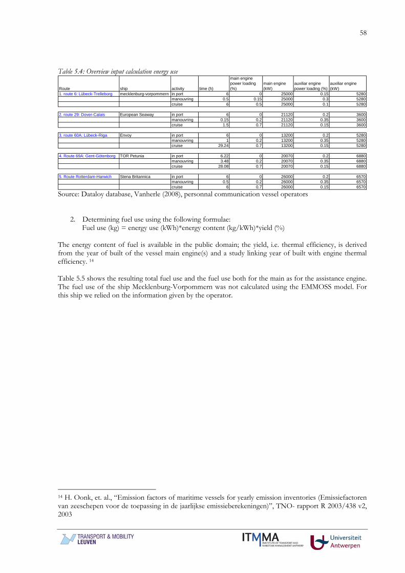
58

Table 5.4: Overview input calculation energy use

Route ship activity time (h)

main engine power loading (%)

main engine (kW)

auxiliar engine power loading (%)

auxiliar engine (kW)

1. route 6: Lübeck-Trelleborg mecklenburg-vorpommern in port 6 0 25000 0.15 5280manouvring 0.5 0.15 25000 0.3 5280cruise 6 0.5 25000 0.1 5280

2. route 29: Dover-Calais European Seaway in port 6 0 21120 0.2 3600manouvring 0.15 0.2 21120 0.35 3600cruise 1.5 0.7 21120 0.15 3600

3. route 60A: Lübeck-Riga Envoy in port 6 0 13200 0.2 5280manouvring 1 0.2 13200 0.35 5280cruise 29.24 0.7 13200 0.15 5280

4. Route 69A: Gent-Götenborg TOR Petunia in port 6.22 0 20070 0.2 6880manouvring 3.48 0.2 20070 0.35 6880cruise 28.08 0.7 20070 0.15 6880

5. Route Rotterdam-Harwich Stena Britannica in port 6 0 26000 0.2 6570manouvring 0.5 0.2 26000 0.35 6570cruise 6 0.7 26000 0.15 6570

Source: Dataloy database, Vanherle (2008), personnal communication vessel operators

2. Determining fuel use using the following formulae:

Fuel use (kg) = energy use (kWh)*energy content (kg/kWh)*yield (%) The energy content of fuel is available in the public domain; the yield, i.e. thermal efficiency, is derived from the year of built of the vessel main engine(s) and a study linking year of built with engine thermal efficiency. 14 Table 5.5 shows the resulting total fuel use and the fuel use both for the main as for the assistance engine. The fuel use of the ship Mecklenburg-Vorpommern was not calculated using the EMMOSS model. For this ship we relied on the information given by the operator.

14 H. Oonk, et. al., “Emission factors of maritime vessels for yearly emission inventories (Emissiefactoren van zeeschepen voor de toepassing in de jaarlijkse emissieberekeningen)”, TNO- rapport R 2003/438 v2, 2003

59

Table 5.5: Total fuel use

Route ship activityfuel use main engine (ton)

fuel use auxiliar engine (ton)

Total Fuel use (ton)

1. route 6: Lübeck-Trelleborg mecklenburg-vorpommern in port 0.00 1.20 1.20manouvring 0.36 0.20 0.56cruise 14.52 0.80 15.33Total 17.09

2. route 29: Dover-Calais European Seaway in port 0.00 1.09 1.09manouvring 0.13 0.05 0.17cruise 4.41 0.21 4.62Total 5.88

3. route 60A: Lübeck-Riga Envoy in port 0.00 1.61 1.61manouvring 0.54 0.47 1.01cruise 55.14 5.87 61.01Total 63.62

4. Route 69A: Gent-Götenborg TOR Petunia in port 0.00 2.17 2.17manouvring 2.48 2.12 4.60cruise 69.96 7.34 77.30Total 84.07

5. Route Rotterdam-Harwich Stena Britannica in port 0.00 2.00 2.00manouvring 0.46 0.29 0.75cruise 19.36 1.50 20.86Total 23.61

Source: calculations TML Total fuel use provides an important intermediate validation step as vessel operators have a fairly good idea of the fuel consumption of vessels active on these routes. The calculated fuel consumption figures have been presented to and accepted by vessel operators.

3. Calculating the emissions using the following formulae: Emissions (kg) = fuel use (kg)* emission factor (kg/kg)*correction factor15

The emission factors in EMMOSS are based on a Dutch study16 and depend on the type of motor, building year, used fuel and the power loading. The required data for the vessels on the selected routes are taken from the Lloyds vessel database. The result of this calculation is emissions in kg for all routes. Figure 5.1 shows the emissions of air pollutants by the vessel on the short sea shipping routes for both the reference case as for the simulation. Given the order of magnitude, we show the effect on CO2 emissions separately in Figure 5.2. In the simulation - 0.5% sulphur content we only see an effect on sulphur emissions as the fuel type (HFO) remains the same. The requirement of 0.1% sulphur content leads to a switch to MDO fuels and hence also influences the other pollutants. Overall, the influence of the revised MARPOL Annex VI on the SO2 emissions is very clear from this picture. Relatively, the impact is larger for long distance routes. The main reason for this is that the relative importance of emissions at berth (which are the same in all scenarios as the regulation of 0.1% sulphur content is already required at berth) is lower.

15 This correction factor is used at low power loading: if the power loading is smaller than 50%, the emission per unit of power increases because the motor is used suboptimal. This varies strongly between pollutants. H.Oonk, ea (2003) 16 H. Oonk, et. al., “Emission factors of maritime vessels for yearly emission inventories (Emissiefactoren van zeeschepen voor de toepassing in de jaarlijkse emissieberekeningen)”, TNO- rapport R 2003/438 v2, 2003

60

Figure 5.1. Emissions Air Pollutants Short Sea Shipping on selected route (kg)

0.00

1000.00

2000.00

3000.00

4000.00

5000.00

6000.00

7000.00

8000.00

9000.00

10000.00

RE

F

SIM

_0.5

SIM

_0.1

RE

F

SIM

_0.5

SIM

_0.1

RE

F

SIM

_0.5

SIM

_0.1

RE

F

SIM

_0.5

SIM

_0.1

RE

F

SIM

_0.5

SIM

_0.1

1.1 route 6: Lübeck-Trelleborg

2. route 29: Dover-Calais 3. route 60A: Lübeck-Riga 4. Route 69A: Gent-Götenborg

5. route Rotterdam-Harwich

Emis

sion

s (k

g) VOSPM10SO2NOxCO

Source: own calculations TML As the type of fuel (HFO) remains the same as in the reference scenario in the simulation where a sulphur content of 0.5% is assumed, there is also no effect on CO2. The revised regulation towards 0.1% sulphur content does require a change to MDO and hence has a – limited- effect on CO2. Non CO2 GHG’s are not considered in this study as they take up less then 5% of total Greenhouse Gasses. We also did not consider the additional CO2 emitted by the additional refinery processing of the distillate which is needed in the simulations. Including these emissions would increase the CO2 emissions in the simulation with a few %, but it will not alter the conclusions.

61

Figure 5.2. CO2 emissions SSS on selected routes (ton)

0

50

100

150

200

250

300

REF SIM_0.5 SIM_0.1 REF SIM_0.5 SIM_0.1 REF SIM_0.5 SIM_0.1 REF SIM_0.5 SIM_0.1 REF SIM_0.5 SIM_0.1




ton CO2

Source: own calculations TML To obtain the marginal external environmental costs, these emission (in kg) need to be multiplied with a the values (in €/kg) stated in Table A2 of annex 1. These values take into account that the emissions happen at sea, away from densely populated areas. This gives a marginal external cost per ship per trip as shown in Figure 5.3. This figure shows that the most important pollutants – in terms of marginal external costs - are SO2, NOx and PM. On average, total external cost per trip decrease with about 5% when going from 1% S HFO to 0.5% S HFO. Going from 1% S HFO to 0.1%S MDO leads to an average decrease of about 15%. The new guidelines clearly have an influence on the marginal external costs of shipping by decreasing the amount of SO2, and to a smaller extend NOx and PM, emitted.

62

Figure 5.3. Marginal external costs (1000€) per ship per trip

0

20

40

60

80

100

120

REF SIM_0.5 SIM_0.1 REF SIM_0.5 SIM_0.1 REF SIM_0.5 SIM_0.1 REF SIM_0.5 SIM_0.1 REF SIM_0.5 SIM_0.1




1000 euro

VOSPM10SO2NOxCO2CO

.

5.2. Marginal external costs of trucks For the marginal external costs of trucks we rely on data which was also used within the GRACE project17. Based on literature and the results of other deliverables the marginal external costs for all modes were calculated18 within this project. Given the distances we assume that a truck type >32 ton is used. The average loading assumed for this type of trucks is about 12 ton. Ideally, the marginal external costs for the specific routes traveled on are used. This would take into account specific characteristics of those routes such as, for example, severe congestion. However, this data is not available. Hence, averaged data was used. For each country we have data for the marginal external costs. They are averaged for the truck fleet of each country. Hence countries with more Euro IV trucks will have a lower marginal external cost per vehiclekm (vkm). There are two options in calculating these costs for the routes using average data: • either one average marginal external costs figures is used and multiplied over the whole distance to

obtain the total marginal external cost of that route • or the country specific marginal cost figure which is multiplied with the number of km traveled

through this country. We have opted for the second option as the marginal external environmental, congestion and accident cost depends more on the country population affected than on the type of truck. 17 Proost ea (2008) FP6 GRACE Deliverable 9: The socio- economic impacts of transport pricing reforms 18 Within this project the TREMOVE model18 was used to analyze a series of policy options with respect to internalizing external cost. The calculated marginal external costs served as an input for these analyses.

63

Table 5.6 shows the marginal external costs in €/vkm for truck >32 ton for the countries involved. The values stated here, lie in the range of the values stated in the IMPACT Study (2008). Table 5.6. Marginal external costs in euro per truckkm for trucks >32 tons marginal external costs infrastructure congestion greenhouse_gas non_greenhouse_gas accidents noise totalBE 0.034 0.146 0.073 0.104 0.073 0.042 0.472DE 0.034 0.089 0.071 0.170 0.030 0.059 0.452DK 0.034 0.047 0.081 0.075 0.063 0.376 0.677FR 0.034 0.226 0.072 0.125 0.089 0.063 0.610NL 0.034 0.050 0.088 0.158 0.051 0.222 0.605NO 0.034 0.174 0.087 0.044 0.032 0.376 0.749SE 0.034 0.186 0.088 0.045 0.016 0.019 0.388UK 0.034 0.159 0.073 0.069 0.037 0.030 0.403LT 0.036 0.012 0.082 0.036 0.076 0.358 0.601LV 0.033 0.010 0.075 0.026 0.084 0.340 0.569PL 0.034 0.017 0.088 0.089 0.066 0.376 0.671EE 0.034 0.012 0.075 0.017 0.048 0.282 0.468 Source: calculations TML for the GRACE project19

5.3. Marginal external cost of rail For the alternative using the Channel tunnel between Dover and Calais, the marginal external costs of electric rail is needed. We will use the average value of an electric train of the UK and France. Table 5.6 shows the marginal external costs per vkm for the UK, France and the average value. Table 5.6. Marginal external costs in euro per vkm for electric rail marginal external costs infrastructure congestion greenhouse_gas non_greenhouse_gas accidents noise totalFR 0.546 0.000 0.094 0.037 0.266 0.152 1.095UK 0.576 0.000 0.223 0.051 0.254 0.034 1.139Average 0.561 0.000 0.159 0.044 0.260 0.093 1.117 Source: calculations TML for the GRACE project20

5.4. Marginal external cost of the selected routes – no modal shift.

In this section we calculate the marginal external cost per truck using either the truck only or the Short sea/truck option for each origin destination pair. For the truck only option we multiplied the number of vkm in each country with the respective marginal external cost of that country. The vkm correspond with the once used in the previous sections and stated in table 4.9. For the truck/rail combination, we make the sum of the marginal external cost of the road section and the marginal external cost of the rail section. The marginal external costs for the road section are calculated as

19 We did not take over the value used for noise for the Netherlands as it clearly fell outside the range found in literature. Based on the ECMT (1998), it was estimated that the marginal external noise cost was 3.532 euro/vkm for the Netherlands. This is about 10 times larger than the costs in other countries. Hence, different from the GRACE study, we decided to use the European average for the cost of noise for the Netherlands. 20 We did not take over the value used for noise for the Netherlands as it clearly felt out of the range found in literature. Based on the ECMT (1998), it was estimated that the marginal external noise cost was 3.532 euro/vkm for the Netherlands. This is about 10 times larger than the costs in other countries. Hence, different from the GRACE study, we decided to use the European average for the cost of noise for the Netherlands.

64

before by multiplying the distance with the country values. For the rail section, we first need to recalculate the value per vkm to a value per truckkm in order to make a fair comparison. To obtain this value we assumed an average loading of 20 trucks per train. The maximum capacity of one Eurostar Freight rail train is 30 trucks21. We then obtain a value of 0.056 € per truckkm using electric rail, which is lower than the marginal external costs of trucks and of Short seavessels. This value is than multiplied with the distance traveled using the Eurostar. For the alternative using short sea shipping, we again make the sum of the road part and the part traveled via short sea. Also for short sea shipping we need to recalculate the value per ship for the whole route to a value for a truck. This was done by dividing the total marginal cost per ship through the average number of trucks on each ship. Note that this is an overestimation for vessels which also transport passengers as it implies that we allocate the full external costs of short sea shipping completely to the freight transported. The importance of this assumption depends on the relative shares of passengers/freight transported. However, it is practically impossible to determine the share of external costs which need to be attributed to passengers and which part to freight traffic. The average number of trucks on a ship was determined by multiplying the maximum capacity with the average utilization rate. For short routes we assumed that 40% of the capacity is used. For medium routes we used 60% utilization and for long routes a utilization rate of 75%. This is also shown in Table 5.7. Table 5.7: Average loading factor

Route shipmaximum number of trucks/ship utilization rates

average number of trucks/ship

1. route 6: Lübeck-Trelleborg mecklenburg-vorpommern* 147 60% 88

2. route 29: Dover-Calais European Seaway 100 40% 40

3. route 60A: Lübeck-Riga Envoy 92 75% 69

4. Route 69A: Gent-Götenborg TOR Petunia 192 75% 144

5. Route Rotterdam-Harwich Stena Britannica 160 60% 96 We can then compare marginal external costs for each origin-destination using either the truck only option or the Short sea/truck combination. For Calais-Dover and Rotterdam-Harwich, the truck only option assumes the use of the Channel Tunnel. The comparison is made in the Table 5.8 below, where the first column states total external costs only using road/rail and the last three columns show total external costs using short sea shipping for the three scenario’s: the reference case, the simulation with 0.5% sulphur and the simulation with 0.1% sulphur. Note that this is a ceteribus paribus comparison, this is, we do not assume any modal shifts away from short sea shipping.

21 http://www.eurotunnel.com/ukcP3Main/ukcCorporate/ukcTheGroup/ukcOperations/ukpTruckShuttles

65

Table 5.8: Marginal external costs (1000 euro) per truck on the different routes for the different modes – no modal shift

1000 euro Origin Destination Road SSS - RefSSS-SIM_0.5 no modal shift

SSS-SIM_0.1 no modal shift

1. Travemünde-Trelleborg 1.1 Dortmund Götenborg 58.86 47.02 46.60 45.431.2 Dortmund Stockholm 84.49 69.69 69.27 68.10

2A. Dover-Calais 2A.1 Rotterdam Tilbury 8.48 15.58 15.26 14.312A.2 Roterdam Londen 8.88 15.98 15.67 14.722A.3 Rotterdam Portsmouth 10.27 17.37 17.05 16.102A.4 Düsseldorf Tilbury 9.99 17.09 16.77 15.822A.5 Düsseldorf Londen 10.39 17.49 17.18 16.232A.6 Düsseldorf Portsmouth 11.78 18.88 18.56 17.612A.7 Brussel Tilbury 6.03 13.13 12.81 11.862A.8 Brussel Londen 6.43 13.53 13.22 12.272A.9 Brussel Portsmouth 7.82 14.92 14.60 13.652A.1 Dortmund Tilbury 10.93 18.03 17.71 16.76

2A.11 Dortmund Londen 11.33 18.43 18.11 17.162A.12 Dortmund Portsmouth 12.72 19.82 19.50 18.552A.13 Rotterdam Manchester 14.28 21.38 21.07 20.122A.14 Dusseldorf Manchester 15.79 22.89 22.58 21.632A.15 Brussels Manchester 11.83 18.93 18.62 17.672A.16 Dortmund Mancester 16.73 23.83 23.51 22.56

2B: Rotterdam-Harwich 2B.1 Rotterdam Tilbury 20.35 33.95 32.52 29.862B.2 Roterdam Londen 21.32 34.68 33.25 30.592B.3 Rotterdam Portsmouth 24.65 39.90 38.47 35.812B.4 Düsseldorf Tilbury 23.97 46.38 44.94 42.282B.5 Düsseldorf Londen 24.94 47.11 45.68 43.022B.6 Düsseldorf Portsmouth 28.27 52.33 50.90 48.242B.7 Brussel Tilbury 14.47 41.39 39.96 37.302B.8 Brussel Londen 15.44 42.12 40.69 38.032B.9 Brussel Portsmouth 18.77 47.35 45.92 43.262B.1 Dortmund Tilbury 26.22 46.66 45.23 42.57

2B.11 Dortmund Londen 27.19 47.39 45.96 43.302B.12 Dortmund Portsmouth 30.52 52.62 51.19 48.532B.13 Rotterdam Manchester 34.28 45.20 43.77 41.112B.14 Dusseldorf Manchester 37.90 57.63 56.20 53.542B.15 Brussels Manchester 28.40 52.65 51.22 48.562B.16 Dortmund Mancester 40.15 57.92 56.49 53.82

3. Lübeck-Riga 3.1 Dieppe Tallinn 90.35 90.99 89.33 89.083.2 Dieppe Kaunas 76.92 92.50 90.84 90.583.3 Antwerp Tallinn 84.30 77.33 75.67 75.413.4 Antwerp Kaunas 70.13 78.84 77.18 76.923.5 Amsterdam Tallinn 85.98 77.93 76.26 76.013.6 Amsterdam Kaunas 64.65 79.43 77.77 77.513.7 Hamburg Tallinn 73.55 58.73 57.07 56.823.8 Hamburg Kaunas 52.25 60.24 58.58 58.323.9 Esbjerg Tallinn 86.89 70.63 68.97 68.72

3.10 Esbjerg Kaunas 63.88 72.14 70.48 70.224. Gent-Götenborg 4.1 Rotterdam Oslo 116.47 135.38 129.96 120.17

4.2 Rotterdam Stockholm 113.50 139.17 133.75 123.96 Source: calculations TML In the reference case SSS leads to less marginal external costs for certain routes. This is the case for the route Travemünde-Trelleborg and for certain origin-destinations using the routes Lubeck-Riga. The loading factor of the ship is quite important here as the loading factor determines over how many trucks the total external cost of the ship can be divided. The assumption of attributing all external costs of RoRovessels to freight also makes that – in the cases where also passengers are transported – the external costs of the short sea/truck alternative are overestimated. For the route going through Calais-Dover, the difference is always in favour of the road alternative as electric rail has very low external costs. The detour that has to be made for some origin-destination pairs to use the Channel Tunnel does not outweigh this. In the simulation, the case becomes more favourable for SSS. The gap significantly reduces and in one case even reverses. However, in general the regulation will not lead to a reversal with respect to external costs if there is no modal shift. However, if there is a modal shift, the picture could be different. This is discussed in the next section.

66

5.5. Marginal external cost of the selected routes – if modal shift.

As was shown in the previous chapters, the new IMO requirements have an effect on costs and prices of short sea shipping and this could lead to a modal shift. The goal of this section is to show the effects on external costs if such a modal shift would take place. In order to do this we calculated total external costs for each origin-destination pair for

- the reference case (1%S HFO) - ref - a simulation (0.5%S HFO) with no modal shift. No modal shift is assumed for this scenario

as a requirement of 0.5% sulphur does not require a change in the type of fuel and hence no strong price increase is expected. – SIM_0.5 no modal shift

- a simulation (0.1%S MDO) with no modal shift – SIM_0.1 no modal shift - a simulation (0.1%S MDO) with 10% modal shift – SIM_0.1 10% modal shift - a simulation (0.1%S MDO) with 20% modal shift – SIM_0.1 20% modal shift - a simulation (0.1%S MDO) with 30% modal shift – SIM_0.1 30% modal shift

Consider, for example, in Figure 5.4 route Lübeck-Trelleborg for trucks departing at Dortmund and arriving in Gotenburg. We assumed 88 trucks on the ship Mecklenburg-Vorpommern. In order to ease the comparison we assume that all 88 trucks are leaving at Dortmund and arriving in Gotenburg. Of course, in reality a mixture of origin-destinations will be present. We can then calculate the total external costs for these trucks when they would all use the truck only option, when they would all use a short sea/truck combination in the reference case and for the simulations, assuming no modal shift. The results are shown in the first 4 bars in figure 5.4. For this origin-destination, the external costs are the higher for the truck only option than for the short sea/truck combination. Of course, in the simulations the total marginal external costs decrease. In the case of modal shift of 10% we assume that 79 trucks will keep on using the short sea/truck combination, while 8 would use shift to the truck only option. The external cost of these 9 trucks is then added to the total external costs. For a modal shift of 20%, 17 trucks are added to the road, etc. Some strong assumptions are used within this calculation. We assume that if drivers decide not to use the short sea/truck combination, they will use the truck only option. They could also opt to minimize the distance using short sea shipping or – in the long run - they could opt to change the logistic process completely and – for example – only 4 trucks would opt for the truck only option. We also assume that the frequency of trips of the ships remains the same. For long distances, where the utilisation is already high (75%) this assumption makes sense. However, for short distances, it could be possible to decrease the frequency. This could have two effect. Or this lower level of service is seen as very bad, and even more trucks move away from short sea shipping. Or it would lead to a higher utilization rate – meaning that total external costs of shipping would be shared by more trucks. As the effect is not clear, we assume that that the level of service remains constant. It is clear from figure 5.5, that assumes a modal shift of 10% in the scenario with 0.1% sulphur leads to a total marginal costs which is higher than in the reference case with 1% sulphur.

67

Figure 5.5: Total marginal external costs (1000 euro) for Dortmund-Götenburg for the different modes – if modal shift

0

10

20

30

40

50

60

70






scenario

1000

Eur

o

SSSRoad

Figure 5.6 shows the case of Rotterdam-Tilbury via Dover-Calais, while Figure 5.7 shows the same case but for the Rotterdam-Harwich route. In Figure 5.6, the distance travelled via the road is the same in both the road/rail option and the short sea/truck combinations. As the external costs of electric rail are very low, the difference between the external costs of the option truck only are only slightly higher than the ‘truck part’ in the short sea/truck combinations. For the exact magnitudes we refer to annex 2. Note that total external costs using road/rail option is higher in Figure 5.7 than in Figure 5.6. This is caused by the fact that we multiplied with the assumed number of trucks on the vessel (40 trucks for Dover-Calais and 96 trucks for Rotterdam-Harwich). In both cases a modal shift of about 20% almost completely mitigates the effect of lowering the sulphur content of fuels.

68

Figure 5.6: Total marginal external costs (1000 euro) for Rotterdam-Tilbury via Dover-Calais for the different modes – if modal shift

0

2

4

6

8

10

12

14

16

18






scenario

1000

eur

o

SSSRoad

Figure 5.7: Total marginal external costs (1000 euro) for Rotterdam-Tilbury via Rotterdam-Harwich for the different modes – if modal shift

0

5

10

15

20

25

30

35

40






scenario

1000

eur

o

SSSRoad

69

Figure 5.8 shows the case of Amsterdam-Talinn for the Lübeck-Riga route. The same conclusions as for Dortmund-Götenburg can be made. Figure 5.8 Total marginal external costs (1000 euro) for Amsterdam-Talinn for the different modes – if modal shift

0

20

40

60

80

100

120






scenario

1000

eur

o

SSSRoad

Figure 5.9 shows the results for Rotterdam-Oslo for the Ghent-Götenborg route. For this route a 10% modal shift leads to external costs which are still lower than in the reference case, but are about at the same level as in the case where 0.5% sulphur and no modal shift is assumed. If the modal shift would be 20%, total external costs are higher than in the reference case. The same information is summarized for all origin-destinations in a table in annex 2.

70

Figure 5.9: Total marginal external costs (1000 euro) for Rotterdam-Oslo for the different modes – if modal shift

0

20

40

60

80

100

120

140

160






scenario

1000

eur

o

SSSRoad

Annex 2 shows the results for all routes. From this analysis, taking into account the assumptions, it can be seen that for 26% of the cases analysed, the gain in marginal external costs due to a decrease in sulphur content to 0.1% will deteriorate compared with the present situation if a modal shift of 10% occurs. If a modal shift of 20% occurs this is the case for almost all origin-destinations. The analysis also shows that if we assume that a decrease in sulphur content to 0.5% would not lead to a modal shift, the total marginal external costs are lower for all routes than if sulphur content would equal 0.1% and a modal shift of about 20% would occur. The analysis of this section and the results in annex 2 show – even when taking into account the assumptions made- that when assessing the effects of a measure on external costs, one should also take into account that some costs are not removed, but shifted to other modes and might even increase.

6. Conclusions and policy recommendations This report aimed at analyzing the potential impact of the new low sulphur requirements on shipping in the ECAs, with an emphasis on short sea shipping. The report particularly focuses on three research questions: (1) What is the expected impact of the new requirements of IMO on costs and prices of short sea traffic in the ECAs? (2) What is the expected impact of the new requirements of IMO on the modal split in the ECAs? (3) What is the expected impact of the new requirements of IMO on external costs? Regarding the first research question, it became clear the effect of the new Annex VI agreement may be quite costly for the participants in the shipping industry. Based on historical price differences, the use of MGO (0.1%) could well imply a cost increase per ton of bunker fuel of on average 80 to 100% (long-term) compared to IFO 380 and 70 to 90% compared to LS 380 grades (1.5%). This conclusion is in line with previous studies. The impact on shipping lines’ cost base when shifting from HFO (1.5%) to MGO

71

would be considerable as well: a 25.5% increase in ship costs for the base scenario and even 30.6% on average for the high scenario with for a number of routes peaks of 40%. These figures only relate to vessels with an average commercial speed of 18.5 knots. The average ship cost increase for fast short sea/ropax ships (25 to 30 knots on average) is estimated at 29% for the low scenario and even 40% (ranging from 31% to 47%) for the high scenario. A shift from HFO (1.5%) to MGO (0.1%) would as such have a large impact on freight rates. The freight rate is defined here as the total unit price customers pay for using the short sea service (typically per 17 lane meters – equivalent to a truck/trailer combination). For traditional short sea services freight rate increases are estimated to reach 8 to 13% for the low scenario and around 20% for the high scenario. For fast short sea services the figures are much higher: on average 25% for the low scenario and 40% for the high scenario. It must be stressed that all of the above figures are averages and that quite substantial differences might occur among the different liner services. A survey was conducted to assess the perception of short sea operators on the potential volume losses and modal shift impacts linked to the implementation of strict low sulphur fuel requirements under different scenarios regarding fuel price evolutions. For the scenario of USD 500 per ton of MGO, the respondents expect freight rate increases in the order of 15 to 25% with an overall average of nearly 18%. The corresponding volume losses are expected to reach 14.5%. For the high scenario (USD 1000 per ton of MGO), the expected impacts are considerable: a freight rate increase of up to 60% and anticipated volume losses of more than 50%. The medium-distance routes would be worst hit. A detailed comparative cost analysis made it possible to assess modal competition between several short sea/truck routing options and the ‘truck only’ option on thirty origin-destination routes linked to the ECAs. All these short sea solutions face potential competition from a ‘truck only’ option (for Dover-Calais in combination with the Channel Tunnel). The use of MGO is expected to increase the transport prices particularly on the origin-destination relations with a medium or long short sea section. Such a price development might eventually trigger a shift from medium and long short sea routes to shorter short sea routes or a ‘truck only’ alternative without any short sea section. The situation is rather precarious on most of routes considered. The cross channel short sea business for manned truck/trailer combinations is likely to be hit hard by the use of MGO. The use of MGO could well imply the end of the transport of manned truck/trailer combinations per vessel across the southern part of the English Channel. The transport connections between Western Europe and the Baltic States are expected to be heavily affected as well. Long-distance short sea services are likely to lose a lot of their appeal to customers. At present, the short sea connections between the Benelux/Western Germany and Scandinavia (Sweden and Norway in particular) face rather limited competition from road haulage. The main competitor is the much shorter short sea link between Travemünde and Trelleborg (which involves much longer trucking distances). However, the use of MGO is expected to narrow down the cost advantage of the long-distance short sea option to such an extent that some customers might start opting for trucking goods instead of using short sea services. More certain is that the use of MGO will trigger a shift from long-distance to short-distance short sea links. The observed shifts in price differences incurred when introducing MGO (0.1%) as a base fuel in the ECAs would undoubtedly lead to changes in the modal split at the expense of short sea services. We also indicated that on some routes shifts from long-distance to short-distance short sea routes are to be expected. Even relatively small traffic losses (e.g. 10% to 20% less cargo) for existing short sea services can trigger a vicious cycle of capacity reduction and lower frequencies ultimately leading to a poorer position for short sea services and thus an unattractive market environment for investors. Vicious cycles characterized by the downsizing of short sea activities and the closures of lines can lead to an overall implosion of a short sea sub-market, leaving room to the ‘truck only’ option or short sea services on short or ultrashort distances to fill the gap in the market. The third section of the report focuses on the third research question: ‘What is the expected impact of the New requirements of IMO on external costs?’. Using the methodology described in the report, we

72

calculated the total marginal external costs for each origin-destination pair. In general, marginal external costs are lower for the short sea/truck combination for some routes, but not for all. However, it should be noted here that for vessels which also transport passengers, the external costs for the short sea vessels are overestimated. If no modal shift is assumed, marginal external costs of short sea vessels of course decrease due to the new requirements. If the effect of a possible backshift is taken into account, even a modal shift of about 10-20% could completely mitigate the initial effect of lowering the emissions. The analysis also showed that if we assume that a decrease in sulphur content to 0.5% would not lead to a modal shift, the total marginal external costs are lower for almost all routes than if sulphur content would equal 0.1% and a modal shift of about 20% would occur. Even when taking into account the assumptions made for this analysis, it is clear that when assessing the effects of a measure on external costs, one should also take into account that some costs are not removed, but shifted to other modes. In summary, the use of MGO (0.1%) is expected to have a negative effect on freight rates and the modal split on a large set of origin-destination relations. On some trade routes the short sea option might lose its appeal to customers. This will lead to traffic losses for the short sea option in favour of trucking. Obviously, the use of MGO will have a positive impact on external costs generated by short sea vessels alone. Depending on the actual modal back shift the overall outcome for the environmental performance might well be negative.

73

References Cofala, J. ea (2007), Analysis of Policy Measures to Reduce Ship Emissions in the Context of the Revision of the National Emissions Ceilings Directive, IIASA for EC DG ENV De Ceuster G. ea (2005), TREMOVE 2.30 Model and Baseline Description, report to EC-DG Environment, Leuven De Ceuster, G. ea (2006), TREMOVE 2 Service contract for the further development and application of the TREMOVE transport model – Lot 3/PART 4: Maritime model and policy runs, Transport & Mobility Leuven for EC DG ENV De Jonge, E. ea (2005), Service Contract on ship emissions: assignment, abatement and market-based instruments, task 2, ENTEC for EC DG ENV DNV Maritime (2006), MARPOL Annex VI: operation in SOX Emission Control Areas, how to comply?, DNV Maritime ECMT (1998), Efficient Transport for Europe, Policies for Internalization of External Costs. European Commission – Directorate General Environment (2002), Advice on impact of reduction in sulphur content of marine fuels marketed in the EU, Study/C.1/01/2002, Brussels ExternE http://www.externe.info/ Fraser, A. (2005),SECA and Future Implications, WISTA Conference Hamburg - September 2005 Friedrich, R; Bickel, P (2001), Environmental External costs of Transport, Clean Air For Europe, http://www.cafe-cba.org Guihéry, L. (2008), International road freight transport in Germany and the Netherlands: driver costs analysis and French perspectives, European Transport Conference, Noordwijkerhout, 6-8 October 2008 IMPACT (2008), Handbook on estimation of external costs in the transport sector, CE Delft Krystallon (2008), Sea Water Scrubbing – Does it Contribute to Increased Global CO2 Emissions?, Krystallon, West Sussex:UK Link ea (1999), The Costs of Road Infrastructure and Congestion in Europe, Springer Market Observatory for Energy (2009), Evolution of oil and petroleum product prices and taxation levels during the year 2008 in the European Union Mayeres, I. (2002), Taxes and Transport Externalities, ETE- working paper 2002-11 Oonk, H. ea (2003), Emission factors of maritime vessels for yearly emission inventories (Emissiefactoren van zeeschepen voor de toepassing in de jaarlijkse emissieberekeningen), TNO-Rapport R 2003/438 v2. Proost ea (2008), The socio-economic impacts of transport pricing reforms, Deliverable 9 of GRACE (Generalisation of Research on Accounts and Cost Estimation), Funded by Sixth Framework Programme. ITS, University of Leeds, Leeds.

74

Skema (2010), Impact Study of the future requirements of Annex VI of the MARPOL Convention on Short Sea Shipping, project supported by the European Commission, Directorate-General for Energy and Transport Starcrest Consulting Group (2005), Evaluation Of Low Sulfur Marine Fuel Availability – Pacific Rim, Starcrest, July 2005 Swedish Forest Industries Federation (2009), Information Paper – Consequences for the Pulp and Paper Industry due to New Sulphur Regulations for Ships, 18 June 2009 Swedish Maritime Administration (2009), Consequences of the IMO’s new marine fuel sulphur regulations, 14 May 2009, 83 p. Vanherle K. ea (2007), Emmission model shipping and rail Flanders; EMMOSS report for VMM, Leuven Vanherle K (2008), Emissie Race: SSS vs. Road, report to Promotion Short sea Shipping Flanders, Leuven

75

Annex 1 This section focuses on the methodology for calculating the marginal external costs. We start with some general explanation on what marginal external costs are. Next, we discuss the marginal external costs which will be used to calculate the effect on external cost of the revised MARPOL Annex VI in 2015. What are marginal external costs? If the cost of an effect is not incorporated into the price for mobility it is considered an external cost. These costs consist not only of costs in monetary sense, but also of, for example, time losses, pollution, etc. We should distinguish marginal external costs from average external costs. Marginal external costs are the additional costs incurred by an extra trip that are not borne by the user himself but by others (Mayeres, 2002). The average external costs are the total external costs divided by the number of users. Except for environmental costs, the average external costs will be very different than the marginal external costs. In this study we focus on the four main categories of externalities22: congestion, accidents environmental costs (including air pollution, global warming and noise) and infrastructure. These are effects resulting directly from actual transport activity. Not all costs are important for all modes. Shipping, for example, does not really have marginal external accident costs. The next sections give an overview of the general methodology applied for marginal external cost calculation. This is, the methodology for air pollution impacts, global warming, the effects of noise, the treatment of accidents and congestion. Marginal external congestion costs There are numerous kinds and causes for congestion. For example (a) changes in road capacity due to unplanned events such as an accident, (b) changes in road capacity due to planned events such as road works and (c) demand exceeding design capacity. In general, the focus lies on the last cause. In this framework, marginal external congestion costs are present whenever an additional vehicle reduces the speed of the other transport users. This decrease in speed will affect the operating costs, the fuel costs and the time cost of the other users. The main cost (90%) is the time losses of the participants (Link ea 1999). The standard approach for the determination of the external congestion costs in economic policy models assumes a static framework and a very simplified spatial environment. It consists of determining, for a given trajectory, the empirical relationship between the traffic flow and the average speed of that flow. This is based on the idea that an increase in traffic flow influences average speed and, therefore, the time needed to make a certain trip. Time losses due to congestion are valued negatively by the travelers. The marginal external congestion cost is then defined simply as the total value of the time losses for the other road users due to an

22 Of course there are other external effects of transport such as effects on ecosystems, visual intrusions, etc. However, these cost elements are fixed with respect to small changes in traffic demand and thus no marginal costs occur.

76

additional vehicle23. Note that the marginal external congestion cost will be very different in the peak and in the off peak. In general, we speak of congestion in the context of road transport. For rail, the volume of traffic is directly controlled by allocation of slots, so capacity should never be exceeded. For rail transport, as there is an operator who manages the tracks; we speak of scarcity of available slots for trains. When the infrastructure approaches capacity, other users are unable to obtain the slot they want. Nevertheless, as traffic approaches capacity, so delays become more frequent. However, as it is possible that compensations are paid, as the effect of the delays depends on the mix of traffic and as values of slots may differ, it is very hard to calculate the marginal external congestion costs for rail. For short sea shipping we do not know of any study trying to estimate the marginal congestion costs. In principle they exist as an additional vessel may increase operation and travel costs. These costs are most likely to occur when entering or leaving the harbour. Hence they are very location specific. As these costs will probably only occur at the beginning and the end of the trip, the relative importance of these costs depends greatly on the length of the trip. Hence, for the analysis we only take into account the marginal external congestion costs for road transport. Marginal external environmental costs The marginal external environmental cost is the environmental damage caused by one more passenger or tonne km. We distinguish between the costs of airborne pollutants and the cost of noise. The methodology used for both is the Impact Pathway Approach, developed in the ExternE project. For airborne pollutants this comprises the steps: • emission calculations. These calculations are based on COPERT III methodologies • dispersion and chemical conversion modeling24 • calculation of physical impacts (on health, buildings, crops, etc. with the help of exposure –response

functions). Methods include the use of series of complex models and databases, as in the cases of acid rain.

• monetary valuation of these impacts (based on willingness-to-pay) Beside the direct emissions from the operation of the vehicle, emissions due to fuel/electricity production are also taken into account. However, we do not take into account the environmental costs of nuclear energy as there are too many uncertainties concerning the valuations and the risks. Hence, we assign a value of zero to the environmental costs of nuclear energy, which could be debated. We also do not take into account the environment damages due to accidental oil spill or chemical spills. The impact-pathway approach makes that the costs will differ from country to country as population, the influence of weather, etc. plays an important role. It also takes into account that the costs will be different for emissions which occur at sea and emissions on land. An exception is the transboundary effects of air

23 In contrast, the average congestion/time costs is defined as total time costs divided by the number of tkm or pkm and is a constant number for all users. This average time cost is not an external cost as people are experiencing this cost. The marginal congestion costs will increase with each user. 24 Ideally, to obtain marginal external costs, the changes in concentration and deposition of primary and secondary pollutants due to the additional emissions caused by the transport of an additional loading unit have to be calculated. The relation between emission and concentration of pollutants may be highly non linear.

77

pollutants and greenhouse gasses (CO2, CH4 and N2O) where the valuations25 are the same over all countries. There are 2 main approaches for determining these values. Either the valuation of global warming due to CO2, CH4 and N2O emissions is based on sustainability criteria for setting specific reduction targets. The Stern report suggests a value of 95 €/tonne26. Another approximation of the external cost can be the price of a CO2 emission permit under the Emission Trading Scheme (ETS) which has been fluctuating between 10 and 30 €/ton over the lasts years. We use the same values as in the GRACE project which are either 8 or 32 €/ton and increasing over time. This value also influences the value of CH4 and N2O. The unit cost values of the SO2, NOx, PM and NMVOS emissions are taken from CAFÉ-EXTERN-E27. Tabel 5.1 gives an overview of the low and high values used in the CAFÉ-EXTERN-E in the countries of the routes analysed. Differences in value are due to population densities, purchasing power which influence the value of a statistical life, etc. We did not have data for Norway. We use the same values as for Sweden. The high values are the values used to value the emissions from trucks and rail. Table A.1: Current valuation of direct and indirect emissions for land transport (€/tonne)

Country CO VOC Nox PM SO2 CO2 N2O

BE HIGH 1 7100 14000 180000 31000 32 9472

LOW 1 2500 5200 61000 11000 8 2368

DE HIGH 0 5100 26000 140000 32000 32 9472

LOW 0 1700 9600 48000 11000 8 2368

FR HIGH 0 4200 21000 130000 23000 32 9472

LOW 0 1400 7700 44000 8000 8 2368

NL HIGH 0 5400 18000 180000 39000 32 9472

LOW 0 1900 6600 63000 13000 8 2368

PL HIGH 0 1900 10000 83000 16000 32 9472

LOW 0 630 3900 29000 5600 8 2368

EST HIGH 0 420 2200 12000 5200 32 9472

LOW 0 140 810 4200 1800 8 2368

DK HIGH 0 2000 12100 48000 15000 32 9472

LOW 0 720 4400 16000 5200 8 2368

LET HIGH 0 650 3700 25000 5700 32 9472

LOW 0 220 1400 8800 2000 8 2368

LIT HIGH 0 710 5000 24000 6800 32 9472

LOW 0 230 1800 8400 2400 8 2368

GB HIGH 1 3200 10000 110000 19000 32 9472

LOW 1 1100 3900 37000 6600 8 2368

NO HIGH 0 980 5900 34000 8100 32 9472

LOW 0 330 2200 12000 2800 8 2368

SW HIGH 0 980 5900 34000 8100 32 9472

LOW 0 330 2200 12000 2800 8 2368 Source: Friederich, R; Bickel, P. (2001)

25 Note that CH4 also has local effects. 26 This value is based on the marginal external cost of CO2 emissions in the A2 basline. The value is produced by using detail integrated assessments models, not sustainability criteria. 27 Friederich, R.; Bickel, P. (2001)

78

Given this information and the relevant emission factors we can then calculate the marginal external environmental costs. In the calculations we also take into account the composition of the fleet (age composition, composition emission standards,… ) in the different countries for the different modes. For short sea we take into account that the emissions happen on sea, away from densely populated areas. Table 5.2 shows the values we use for the Baltic Sea and the North Sea. The difference between them is due to the magnitude of the sea and the surrounding countries. The valuations start from the valuations stated in table 5.1, but use a blame matrix to take into account the place where the pollutant is emitted and the place where the pollutant ends up. Table A.2. Valuation of direct and indirect emissions for the Baltic and the North Sea Sea CO VOC Nox PM SO2 CO2 N2O

Baltic Sea 1 955 7436 26050 2678 32 7436

North Sea 1 2270 12525 8210 6620 8 12524 Source: Tremove Maritime The marginal external noise cost is the valuation of the noise damage associated with one additional trip. It is a local external cost and includes the damage to other users and the damage to the neighbourhood. Noise emissions of transport activities affect humans mainly in two ways: • negative physiological effects such as for example a change in heart rate, blood pressure, inducing

measurable increases in heart attack risk. • negative psychological effects such as annoyance, disturbance of communication and recreation,

insomnia, loss of (mental) productivity. In ExternE the methodology used to quantify the physiological effects followed the impact-pathway approach, which comprises the following steps. • sound emission modelling • sound propagation and exposure of dwellings • quantification of impacts • valuation of impacts. The negative psychological effects are usually valuated using willingness to pay for avoiding annoying noise levels. Note that for short sea shipping the marginal noise costs will be rather small and expected to be negligible, since the noise impact of a vessel is general low and the population density directly located to the waterway is also low. Hence we will not take them into account for short sea shipping. Marginal external accident costs Marginal external accident costs are the incremental costs of an accident borne by society at large, including victims, family and friends, imposed by those who cause the accident risk. Again we focus on road and rail modes. External accident costs of waterborne transport are considered as negligible. The number of accidents with personal injury is very low and the amount of tonne km transported each year is very high.

79

The traditional approach set out by Lindberg (2002, 2006) to calculate the marginal external costs assumes that when an additional road users enters the traffic flow: • he exposes himself to the average accident risk, while he does not take all accident costs into account. • he may have an impact on the accident risk of others (over different modes) and therefore on the

associated costs for society and these other users • other transport users (over different modes) adapt their behaviour when traffic changes. These

avoidance costs should also be taken into account. When economic values are assigned to these three consequences they express the total marginal accident costs (internal and external). We use the same values as used in the GRACE project. Marginal external infrastructure costs The marginal infrastructure costs are the additional infrastructure cost related to an additional vehicle. Again we only consider the marginal external infrastructure cost of road and rail. There are two ways of calculating the marginal external infrastructure cost. If information is available on the average cost and the elasticity, one can simply calculate the marginal cost as the product of the elasticity with the average infrastructure cost. Another option, if no information is available, is to use the variable infrastructure costs as a proxy for the marginal infrastructure costs. In the GRACE project the first method was used.

80

Annex 2: Marginal external costs (1000€) for all origin-destinations if there is modal shift Indicated in blue are the simulation scenarios for short sea shipping/road combinations which the marginal external costs is equal or higher than in the reference case. If numbers are equal in the reference case and in the simulation and this is not marked, this means that the equality of numbers is merely the effect of rounding. marginal external costs (1000 €) per trip Origin Destination Road SSS - Ref



SSS-SIM_0.1 10% modal shift



1. Rostock-Trelleborg 1.1 Dortmund Götenborg Road 58.9 36.5 36.5 36.5 38.7 48.2 50.5Mecklenburg-vorpommern SSS 0.0 10.6 10.1 9.0 9.0 9.0 9.0

Total 58.9 47.0 46.6 45.4 47.7 57.2 59.4

1.2 Dortmund Stockholm Road 84.5 59.1 59.1 59.1 61.7 76.0 78.6SSS 0.0 10.6 10.1 9.0 9.0 9.0 9.0Total 84.5 69.7 69.3 68.1 70.6 85.0 87.5

2.Dover-Calais 2A.1 Rotterdam Tilbury Road 8.5 8.4 8.4 8.4 8.4 10.1 10.1European Seaway SSS 0.0 7.2 6.9 5.9 5.9 5.9 5.9

Total 8.5 15.6 15.3 14.3 14.3 16.0 16.0

2A.2 Roterdam Londen Road 8.9 8.8 8.8 8.8 8.8 10.6 10.6SSS 0.0 7.2 6.9 5.9 5.9 5.9 5.9Total 8.9 16.0 15.7 14.7 14.7 16.5 16.5

2A.3 Rotterdam Portsmouth Road 10.3 10.2 10.2 10.2 10.2 12.2 12.2SSS 0.0 7.2 6.9 5.9 5.9 5.9 5.9Total 10.3 17.4 17.1 16.1 16.1 18.2 18.2

2A.4 Düsseldorf Tilbury Road 10.0 9.9 9.9 9.9 9.9 11.9 11.9SSS 0.0 7.2 6.9 5.9 5.9 5.9 5.9Total 10.0 17.1 16.8 15.8 15.8 17.8 17.8

2A.5 Düsseldorf Londen Road 10.4 10.3 10.3 10.3 10.3 12.4 12.4SSS 0.0 7.2 6.9 5.9 5.9 5.9 5.9Total 10.4 17.5 17.2 16.2 16.2 18.3 18.3

2A.6 Düsseldorf Portsmouth Road 11.8 11.7 11.7 11.7 11.7 14.0 14.1SSS 0.0 7.2 6.9 5.9 5.9 5.9 5.9Total 11.8 18.9 18.6 17.6 17.6 20.0 20.0

2A.7 Brussel Tilbury Road 6.0 5.9 5.9 5.9 5.9 7.1 7.2SSS 0.0 7.2 6.9 5.9 5.9 5.9 5.9Total 6.0 13.1 12.8 11.9 11.9 13.1 13.1

2A.8 Brussel Londen Road 6.4 6.3 6.3 6.3 6.4 7.6 7.6SSS 0.0 7.2 6.9 5.9 5.9 5.9 5.9Total 6.4 13.5 13.2 12.3 12.3 13.6 13.6

2A.9 Brussel Portsmouth Road 7.8 7.7 7.7 7.7 7.7 9.3 9.3SSS 0.0 7.2 6.9 5.9 5.9 5.9 5.9Total 7.8 14.9 14.6 13.7 13.7 15.2 15.2

2A.1 Dortmund Tilbury Road 10.9 10.8 10.8 10.8 10.8 13.0 13.0SSS 0.0 7.2 6.9 5.9 5.9 5.9 5.9Total 10.9 18.0 17.7 16.8 16.8 18.9 19.0

2A.11 Dortmund Londen Road 11.3 11.2 11.2 11.2 11.2 13.5 13.5SSS 0.0 7.2 6.9 5.9 5.9 5.9 5.9Total 11.3 18.4 18.1 17.2 17.2 19.4 19.4

2A.12 Dortmund Portsmouth Road 12.7 12.6 12.6 12.6 12.6 15.2 15.2SSS 0.0 7.2 6.9 5.9 5.9 5.9 5.9Total 12.7 19.8 19.5 18.5 18.6 21.1 21.1

2A.13 Rotterdam Manchester Road 14.3 14.2 14.2 14.2 14.2 17.0 17.1SSS 0.0 7.2 6.9 5.9 5.9 5.9 5.9Total 14.3 21.4 21.1 20.1 20.1 23.0 23.0

2A.14 Dusseldorf Manchester Road 15.8 15.7 15.7 15.7 15.7 18.9 18.9SSS 0.0 7.2 6.9 5.9 5.9 5.9 5.9Total 15.8 22.9 22.6 21.6 21.6 24.8 24.8

2A.15 Brussels Manchester Road 11.8 11.7 11.7 11.7 11.8 14.1 14.1SSS 0.0 7.2 6.9 5.9 5.9 5.9 5.9Total 11.8 18.9 18.6 17.7 17.7 20.0 20.0

2A.16 Dortmund Mancester Road 16.7 16.6 16.6 16.6 16.6 20.0 20.0SSS 0.0 7.2 6.9 5.9 5.9 5.9 5.9Total 16.7 23.8 23.5 22.6 22.6 25.9 25.9

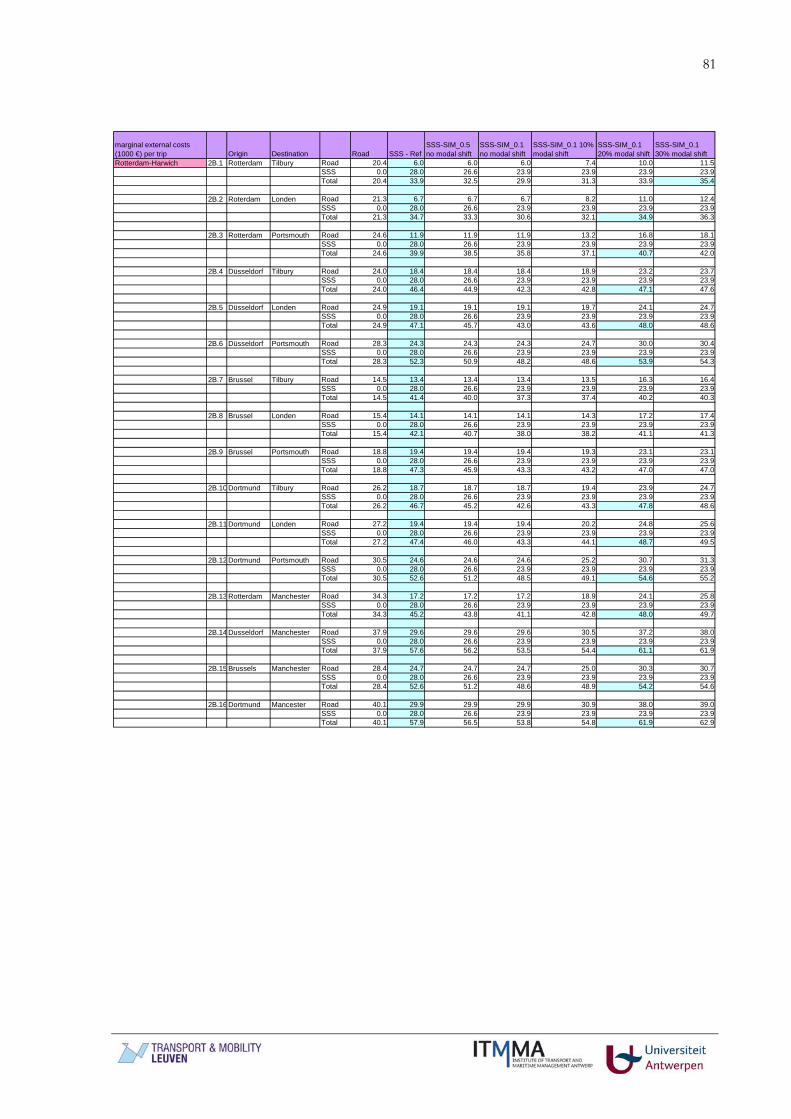
81

marginal external costs (1000 €) per trip Origin Destination Road SSS - Ref






Rotterdam-Harwich 2B.1 Rotterdam Tilbury Road 20.4 6.0 6.0 6.0 7.4 10.0 11.5SSS 0.0 28.0 26.6 23.9 23.9 23.9 23.9Total 20.4 33.9 32.5 29.9 31.3 33.9 35.4

2B.2 Roterdam Londen Road 21.3 6.7 6.7 6.7 8.2 11.0 12.4SSS 0.0 28.0 26.6 23.9 23.9 23.9 23.9Total 21.3 34.7 33.3 30.6 32.1 34.9 36.3

2B.3 Rotterdam Portsmouth Road 24.6 11.9 11.9 11.9 13.2 16.8 18.1SSS 0.0 28.0 26.6 23.9 23.9 23.9 23.9Total 24.6 39.9 38.5 35.8 37.1 40.7 42.0

2B.4 Düsseldorf Tilbury Road 24.0 18.4 18.4 18.4 18.9 23.2 23.7SSS 0.0 28.0 26.6 23.9 23.9 23.9 23.9Total 24.0 46.4 44.9 42.3 42.8 47.1 47.6

2B.5 Düsseldorf Londen Road 24.9 19.1 19.1 19.1 19.7 24.1 24.7SSS 0.0 28.0 26.6 23.9 23.9 23.9 23.9Total 24.9 47.1 45.7 43.0 43.6 48.0 48.6

2B.6 Düsseldorf Portsmouth Road 28.3 24.3 24.3 24.3 24.7 30.0 30.4SSS 0.0 28.0 26.6 23.9 23.9 23.9 23.9Total 28.3 52.3 50.9 48.2 48.6 53.9 54.3

2B.7 Brussel Tilbury Road 14.5 13.4 13.4 13.4 13.5 16.3 16.4SSS 0.0 28.0 26.6 23.9 23.9 23.9 23.9Total 14.5 41.4 40.0 37.3 37.4 40.2 40.3

2B.8 Brussel Londen Road 15.4 14.1 14.1 14.1 14.3 17.2 17.4SSS 0.0 28.0 26.6 23.9 23.9 23.9 23.9Total 15.4 42.1 40.7 38.0 38.2 41.1 41.3

2B.9 Brussel Portsmouth Road 18.8 19.4 19.4 19.4 19.3 23.1 23.1SSS 0.0 28.0 26.6 23.9 23.9 23.9 23.9Total 18.8 47.3 45.9 43.3 43.2 47.0 47.0

2B.10 Dortmund Tilbury Road 26.2 18.7 18.7 18.7 19.4 23.9 24.7SSS 0.0 28.0 26.6 23.9 23.9 23.9 23.9Total 26.2 46.7 45.2 42.6 43.3 47.8 48.6

2B.11 Dortmund Londen Road 27.2 19.4 19.4 19.4 20.2 24.8 25.6SSS 0.0 28.0 26.6 23.9 23.9 23.9 23.9Total 27.2 47.4 46.0 43.3 44.1 48.7 49.5

2B.12 Dortmund Portsmouth Road 30.5 24.6 24.6 24.6 25.2 30.7 31.3SSS 0.0 28.0 26.6 23.9 23.9 23.9 23.9Total 30.5 52.6 51.2 48.5 49.1 54.6 55.2

2B.13 Rotterdam Manchester Road 34.3 17.2 17.2 17.2 18.9 24.1 25.8SSS 0.0 28.0 26.6 23.9 23.9 23.9 23.9Total 34.3 45.2 43.8 41.1 42.8 48.0 49.7

2B.14 Dusseldorf Manchester Road 37.9 29.6 29.6 29.6 30.5 37.2 38.0SSS 0.0 28.0 26.6 23.9 23.9 23.9 23.9Total 37.9 57.6 56.2 53.5 54.4 61.1 61.9

2B.15 Brussels Manchester Road 28.4 24.7 24.7 24.7 25.0 30.3 30.7SSS 0.0 28.0 26.6 23.9 23.9 23.9 23.9Total 28.4 52.6 51.2 48.6 48.9 54.2 54.6

2B.16 Dortmund Mancester Road 40.1 29.9 29.9 29.9 30.9 38.0 39.0SSS 0.0 28.0 26.6 23.9 23.9 23.9 23.9Total 40.1 57.9 56.5 53.8 54.8 61.9 62.9

82

marginal external costs (1000 €) per trip Origin Destination Road SSS - Ref






3. Lubeck-Riga 3.1 Dieppe Tallinn Road 90.4 45.2 45.2 45.2 49.7 63.2 67.7SSS 0.0 45.8 44.2 43.9 43.9 43.9 43.9Total 90.4 91.0 89.3 89.1 93.6 107.1 111.7

3.2 Dieppe Kaunas Road 76.9 46.7 46.7 46.7 49.7 62.0 65.1SSS 0.0 45.8 44.2 43.9 43.9 43.9 43.9Total 76.9 92.5 90.8 90.6 93.6 106.0 109.0

3.3 Antwerp Tallinn Road 84.3 31.5 31.5 31.5 36.8 48.3 53.6SSS 0.0 45.8 44.2 43.9 43.9 43.9 43.9Total 84.3 77.3 75.7 75.4 80.7 92.3 97.6

3.4 Antwerp Kaunas Road 70.1 33.0 33.0 33.0 36.7 47.0 50.7SSS 0.0 45.8 44.2 43.9 43.9 43.9 43.9Total 70.1 78.8 77.2 76.9 80.6 90.9 94.7

3.5 Amsterdam Tallinn Road 86.0 32.1 32.1 32.1 37.5 49.3 54.7SSS 0.0 45.8 44.2 43.9 43.9 43.9 43.9Total 86.0 77.9 76.3 76.0 81.4 93.2 98.6

3.6 Amsterdam Kaunas Road 64.7 33.6 33.6 33.6 36.7 46.5 49.6SSS 0.0 45.8 44.2 43.9 43.9 43.9 43.9Total 64.7 79.4 77.8 77.5 80.6 90.4 93.6

3.7 Hamburg Tallinn Road 73.5 12.9 12.9 12.9 19.0 27.6 33.7SSS 0.0 45.8 44.2 43.9 43.9 43.9 43.9Total 73.5 58.7 57.1 56.8 62.9 71.5 77.6

3.8 Hamburg Kaunas Road 52.2 14.4 14.4 14.4 18.2 24.8 28.6SSS 0.0 45.8 44.2 43.9 43.9 43.9 43.9Total 52.2 60.2 58.6 58.3 62.1 68.8 72.6

3.9 Esbjerg Tallinn Road 86.9 24.8 24.8 24.8 31.0 42.2 48.4SSS 0.0 45.8 44.2 43.9 43.9 43.9 43.9Total 86.9 70.6 69.0 68.7 74.9 86.1 92.3

3.10 Esbjerg Kaunas Road 63.9 26.3 26.3 26.3 30.1 39.1 42.8SSS 0.0 45.8 44.2 43.9 43.9 43.9 43.9Total 63.9 72.1 70.5 70.2 74.0 83.0 86.8

4. Gent-Götenborg 4.1 Rotterdam Oslo Road 116.5 34.1 34.1 34.1 42.3 57.4 65.6SSS 0.0 101.3 95.8 86.1 86.1 86.1 86.1Total 116.5 135.4 130.0 120.2 128.4 143.5 151.7

4.2 Rotterdam Stockholm Road 113.5 37.9 37.9 37.9 45.5 60.6 68.2SSS 0.0 101.3 95.8 86.1 86.1 86.1 86.1Total 113.5 139.2 133.7 124.0 131.5 146.7 154.2

FINAL REPORT ITMMA TML Analysis of the · PDF fileAnalysis of the Consequences of Low Sulphur...

Documents

Transcript of FINAL REPORT ITMMA TML Analysis of the · PDF fileAnalysis of the Consequences of Low Sulphur...