Fin design for MermaidTM podMaster Thesis Project

J ENS N I LSSON JOHAN RUZS ITS

STOCKHOLM2008 -02 -27

Center for Naval Architecture

i

Abstract This master thesis work has been performed at Rolls Royce on one of their propulsion systems the MermaidTM pod. The main purpose of the work is to produce a conceptual design of a fin that reduces the momentum around the steering axis of the pod as far as possible. First a literature study was carried out. This included effects on fin fitted pods, recovery of rotational energy, economics and rules from classification societies. Then the fin was analysed both hydrodynamically and mechanically. The hydrodynamic analysis was performed with linear theory which has been compared with tests results performed by Rolls Royce. The structural analysis, which is based on numerical methods, covered structural arrangement of the fin including interfaces between the pod and the fin. A fin with a NACA 0015 profile, a cord of 1.5 meters, an average length of 1.35 meters and fasten to the pod with a short interface seem to be the best solution considering hydrodynamics, mechanics and economics. The fin should be mounted as far back on the pod as possible at a six a clock position. The size of the fin is dependant of the size of the pod.

ii

Preface This report is a Master Thesis at the Royal Institute of Technology, KTH, Centre for Naval Architecture. The work in this thesis was carried out at Rolls-Royce AB in Kristinehamn during the period June –December 2007. The authors would like to thank: Per Nahnfeldt, supervisor at Rolls-Royce AB, for support and guidance to the authors during their work at Rolls-Royce AB. Anders Rosén, examiner at The Royal Institute of Technology, for his inspiring teaching and encouragement and support during the work. The Personnel at Rolls-Royce Mermaid pod division for valuable comments and opinions on the work and for supporting the authors with specific knowledge on the pod propulsive systems. Not to mention the great working atmosphere that exists at the division. The Personnel at Rolls-Royce Hydrodynamic Research centre for support to the authors during their work. Kristinehamn, December 2007 Jens Nilsson Johan Ruzsits

1

1 Table of content Fin design for MermaidTM pod.................................................................................................... i Abstract ....................................................................................................................................... i Preface........................................................................................................................................ ii 1 Table of content.................................................................................................................. 1 2 Nomenclature ..................................................................................................................... 2

2.1 Structural Design........................................................................................................ 2 2.2 Hydrodynamics .......................................................................................................... 3

3 Introduction ........................................................................................................................ 4 3.1 Effects of fin fitting to pods ....................................................................................... 5 3.2 Design parameters ...................................................................................................... 5

4 Hydrodynamics ................................................................................................................ 10 4.1 Wing theory.............................................................................................................. 10 4.2 Forces on fin............................................................................................................. 14 4.3 Forces on pod ........................................................................................................... 16 4.4 Inflow velocities....................................................................................................... 17 4.5 Analysis.................................................................................................................... 18 4.6 Conclusion................................................................................................................ 27 4.7 Hydrodynamic design .............................................................................................. 28 4.8 Future work .............................................................................................................. 29

5 Structural Design.............................................................................................................. 30 5.1 Introduction .............................................................................................................. 30 5.2 Theory ...................................................................................................................... 32 5.3 Beam model.............................................................................................................. 42 5.4 FEM.......................................................................................................................... 46 5.5 Interface between fin and pod .................................................................................. 50 5.6 Fatigue in welding.................................................................................................... 58 5.7 Conceptual structural design .................................................................................... 60 5.8 Future work .............................................................................................................. 61

6 Economy........................................................................................................................... 62 7 Summary and discussion.................................................................................................. 64

7.1 Hydrodynamic.......................................................................................................... 64 7.2 Structure ................................................................................................................... 64 7.3 Economy................................................................................................................... 65

8 References ........................................................................................................................ 66 8.1 Published material .................................................................................................... 66 8.2 Non-published material ............................................................................................ 67

2

2 Nomenclature 2.1 Structural Design Symbol Unit Description A m2 Enclosed area of profile A m2 Area of section in general a m Plate length b m Plate width c m Cord length in general D Nm Plate flexural rigidity D m Diameter in general d m Diameter in general E Pa Young's modulus F N Force in general G Pa Shear modulus h m Beam height h m Plate thickness Ixx m4 2nd Moment of inertia of x-axis Ixy m4 2nd Moment of inertia of xy-axis Iyy m4 2nd Moment of inertia of y-axis J m4 St-Vernant torsion stiffness K - Buckling coefficient ks - Shear buckling coefficient L m Length in general Li m Lever arm for shear load to shear centre l m Lever arm for shear flow to shear centre N N Normal force in general N m Tool width Nx N/m In-plane load Ny N/m In-plane load Nxy N/m In-plane load M Nm Bending moment Mv Nm Twisting moment m - Buckling mode Pcr N/m Critical in-plane load qb N/m Base shear flow qs N/m Shear flow qs,0 N/m Initial shear flow q N/m Distributed force q Pa Pressure r m Radius in general Sx N Shear load in x-direction Sy N Shear load in y-direction s m Sector coordinate T N Shear force T m Wing profile thickness T' - Wing thickness in percent of cord tf m Beam frame thickness ts m Shell thickness tw m Beam web thickness

3

w m Deflection x m Centre of gravity in x-direction y m Centre of gravity in y-direction δ m Deflection in general ζs m Position of shear centre σ Pa Stress in general τ Pa Shear stress in general Δ - Laplace operator ν - Poisson's ratio ρ kg/m3 Density in general θ ˚ Twist of section ψ ˚ Steering angle μ - Shear factor 2.2 Hydrodynamics Symbol Unit Description AR - Aspect ratio A m2 Lateral planform area CD - Drag coefficient 3D CDi - Induced Drag coefficient 3D cd - Drag coefficient 2D CL - Lift coefficient 3D cl - Lift coefficient 2D D N Drag D m Propeller diameter e - Effectiveness of planform Fx N Force in x-direction Fy N Force in y-direction

J - Number of advance VJn D

=⋅

KMZ - Moment coefficient 2 5z

MZMKn Dρ

=⋅ ⋅

KFx - Thrust coefficient in x-direction 2 4x

FXFK

n Dρ=

⋅ ⋅

KFY - Thrust coefficient in y-direction 2 4y

FY

FK

n Dρ=

⋅ ⋅

L N Lift l m Lever arm Mz Nm Azimuth moment n r/min, r/s Propeller rotational speed

Re - Reynolds number Re Ulρυ

=

s m Span U m/s Free stream velocity V m/s Speed of advance ρ kg/m3 Density of water α ˚ Angle of attack β ˚ Fin angle to pod

4

3 Introduction Rolls Royce manufactures different propulsion systems for marine applications. One of these systems is the MermaidTM pod, seen in Figure 3.1. This system is an azimuthing unit that replaces the common propeller and rudder configuration. The unit has an integrated electric motor directly driving the propeller shaft. When azimuthing this device a momentum is needed. In some cases this momentum around the steering axis gets quite large. A way to reduce this momentum is to fit the pod with a fin. A side effect of this fin is a change in propulsion efficiency.

Figure 3.1. Two pods seen in dry-dock.

A feasibility study has been done by Rolls Royce indicating that certain benefits could be gained by fitting a MermaidTM podded propulsor with a fin to optimize the hydrodynamic behaviour.1 A suitable way to further investigate the fitting of a fin on the MermaidTM pod is this master thesis project. This project should give a suggestion to a conceptual fin design and an idea of the benefits and consequences of this fin.2 The recommendation of a conceptual solution will be in terms of:

• Hydrodynamic design, including profile, planform and tipform which give maximum reduction of the momentum around the steering axis production costs in mind.

1 Johansson, R., New generation pod 2 Specification of master thesis project – Fin Design for MermaidTM pod

5

• Structural arrangement including scantlings of the fin and the pod-fin interface which gives a minimum of production costs and fulfils the requirements of the classification societies and additional requirements from Rolls-Royce.

To fulfil the objectives described above the following aspects should be evaluated during the work:

• Pros and cons of fin fitted pods • Hydrodynamic consequences of fin with respect to propeller efficiency • Mechanical consequences of fin with respect to steering gear equipment • Optimal hydrodynamic design of fin • Optimal design of load transfer from fin to pod housing

3.1 Effects of fin fitting to pods There are advantages and disadvantages of fitting a pod with a fin. The major ones are listed below. Advantages

• Less momentum around steering axis.

• Gain in propulsive efficiency with recovery of the rotational energy.

• Increased steering effects. • Reduced cost of steering

machinery and maintenance cost on it.

Disadvantages • Increased resistance due to extra

drag of the fin. • Increased manufacturing cost,

production and installation. • Increased maintenance costs, due

to fin.

The obvious advantage of the fin is the reduction in momentum around the steering axis. A positive side effect is the recovery of rotational energy that can increase the propulsion efficiency. The efficiency is increased due to that the propeller is working in a more favorable environment. This efficiency increase has to be compared to the efficiency decrease due to the added drag of the fin. The other aspect of this is the costs. If a fin is added to the pod the manufacturing cost will increase. Also the maintenance cost of the fin will be added to the costs. On the other hand the lower momentum around the steering axis will gain lower costs in the steering gear machinery installation and may decrease the maintenance cost to the machinery. It is also possible that the efficiency increases so that the fuel consumption decreases. 3.2 Design parameters To achieve the goal of reducing the momentum around the steering axis and improving the total efficiency of the propulsion system, by the means of adding fins, the involved parameters has to be identified. This has been done thru a literature study. In the case of the reduction of momentum around the steering axis the critical parameters are the perpendicular distance to the steering axis, and the forces acting on the fin. When trying to maximise the propulsion efficiency, which is equivalent to recovering as much rotational energy as possible in the flow, the main parameters are the number of fins their cord length and their axial distance to the propeller. A suitable profile for the different

6

fins also has to be decided so that the increased resistance from the installation is kept on a low level and that the energy in the water is recovered in an efficient way. The geometrical constraints on the fin are that it can not extend further out from the pod housing than the propeller and not further fore or aft than the pod itself. This makes a cylinder in which the fin must fit.

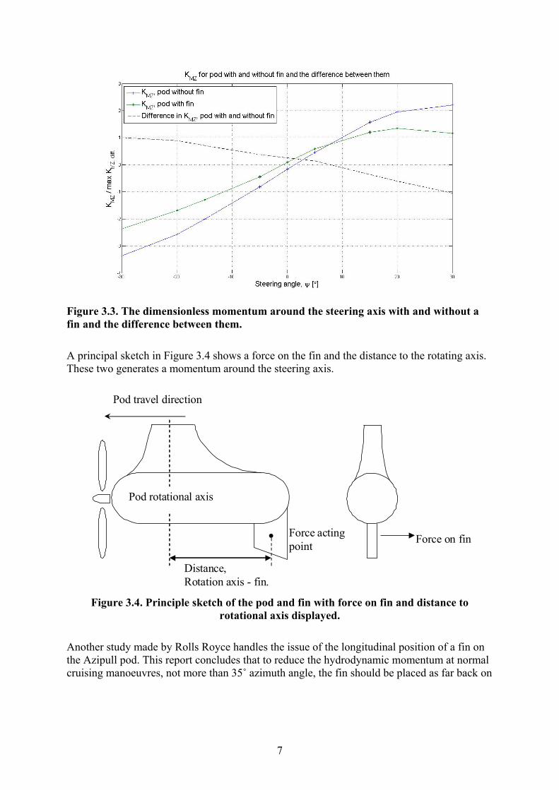
3.2.1 Hydrodynamic momentum Adding a fin to the pod will affect the momentum around the steering axis, MZ, defined in Figure 3.2. The momentum occurs because of the hydrodynamic forces when the pod is travelling trough the water. Figure 3.3 shows the dimensionless momentum needed to keep the pod at a constant steering angle without a fin, with a fin and the difference between them. This momentum will be referred to as hydrodynamic momentum. The steering angel is defined as 0 at straight forward and positive when rotated to the right. It can be seen that the momentum is reduced with the fin.3

FY

FX

MZ

Figure 3.2. Definition of momentum MZ the global pod forces FX, FY are also shown. the

pod is seen from aove.

3 Johansson, R., New Generation Pod

7

Figure 3.3. The dimensionless momentum around the steering axis with and without a fin and the difference between them.

A principal sketch in Figure 3.4 shows a force on the fin and the distance to the rotating axis. These two generates a momentum around the steering axis.

Pod rotational axis

Force on fin• Force actingpoint

Distance, Rotation axis - fin.

Pod travel direction

Figure 3.4. Principle sketch of the pod and fin with force on fin and distance to

rotational axis displayed. Another study made by Rolls Royce handles the issue of the longitudinal position of a fin on the Azipull pod. This report concludes that to reduce the hydrodynamic momentum at normal cruising manoeuvres, not more than 35˚ azimuth angle, the fin should be placed as far back on

8

the pod as possible.4 A fin behind the steering axis will decrease the hydrodynamic momentum needed a fin fore of the axis increases the momentum needed.

3.2.2 Recovery of rotational energy Regarding the recovery of rotational energy in the literature, most investigations of the energy recovery are done by means of a stator or just a rudder. Some of the information provided is still valid for the case of fitting a pod with a fin. A higher number of fins will recover more energy but there is not very much effect gained after about 9 fins have been added, according to Çelik and Güner, but effects from one stator blocking another is not considered. In that study just the propeller efficiency is estimated not the total efficiency of the system after the fins have been added.5 Ishida does a more practical approach based on a total efficiency of the propulsion system and concludes that there is no gain in adding more than 5 fins. Ishida also state that an increase from 2 to 4 fins, which would be the equivalent of fitting a fin horizontally on each side of a rudder, gives a reasonable increase in efficiency in relation to the quite small modification.6 A change in cord length of the fin will change the lift and drag characteristics on the fin. An increase of cord length will increase the drag and slightly decrease the total propulsive efficiency. The change in thrust and torque are quite independent of the cord length. This implies that a short cord is preferred.7 The distance between the propeller and fin is another parameter considered. A thought is that a longer distance would give less rotational energy to recover. But according to Ishida the rotational energy does not dissipate a significant amount at a distance between 0.125 and 2 times the propeller diameter behind the propeller.8 This statement is valid for a propeller slipstream without disturbing objects. Because of the fact that the pod housing and the strut are in the propeller slipstream this may not be valid for this case. Bohm´s model test shows that a fin placed closer to the propeller gives a higher propulsive efficiency.9 This is probably more accurate in this case as the strut and body of the pod will change the flow field approaching the fin.

3.2.3 Economy The primary reason for attaching a fin to the pod is to reduce the power needed in the steering gear equipment. This reduction will hopefully gain that a less expensive installation of the steering gear will be needed. The feasibility study also indicates a higher propulsive efficiency which will reduce the operational costs due to reduction of fuel consumption. However, attaching a fin to a pod will of course result in higher material and production costs, not only in the actual fin but also in the surrounding structure in terms of e.g. additional stiffening systems and redesigning of connections between parts in the pod. The material costs are quite easy to estimate with knowledge of material weight and raw material price. The actual manufacturing costs are depending on the need of advanced 4 Bohm, M. 5 Çelik, F., Güner, M. 6 Ishida, S. 7 Li, D-Q., Gilbert, D. 8 Ishida, S. 9 Bohm, M.

9

production techniques as special tools in the forming process or the rate of complexity in the structure that may require a lot of welding or other sorts of joining techniques.

3.2.4 Classification societies Det Norske Veritas and Lloyd's register, which have rules for pods, have been examined for rules and guidelines for attaching a fin to a pod. The result of the review is unfortunately that none of these two have any guidelines for this type of fin attaching constructions. However there are rules and guidelines for rudders. As comparison this can be a reasonable way of treating the problem. The guidelines are in general based on the ship's service speed and on the global dimensions of the rudder when e.g. forces and plate thicknesses should be estimated. Both societies do accept divergences, in the constructions, from the rules if fairly accurate direct calculations are presented and show that the construction does not fail during operation. The differences between the two classification societies are quite small. The greatest difference, for the same configuration, is the estimated force the rudder is subjected to. Estimated force has a relative difference of about 20% between the societies. As a result of this the difference in bending moment, which the rudder is subjected to, also is about 20%. The strength requirements are almost the same between the societies. The requirements for minimum shell and plate thicknesses are also approximately equal between the societies.10 In general DNV rules have been used due to DNV prescribe lower allowed stress levels.

10 DNV chap: 3.3.2. and Lloyd's chap: 3.13.2.

10

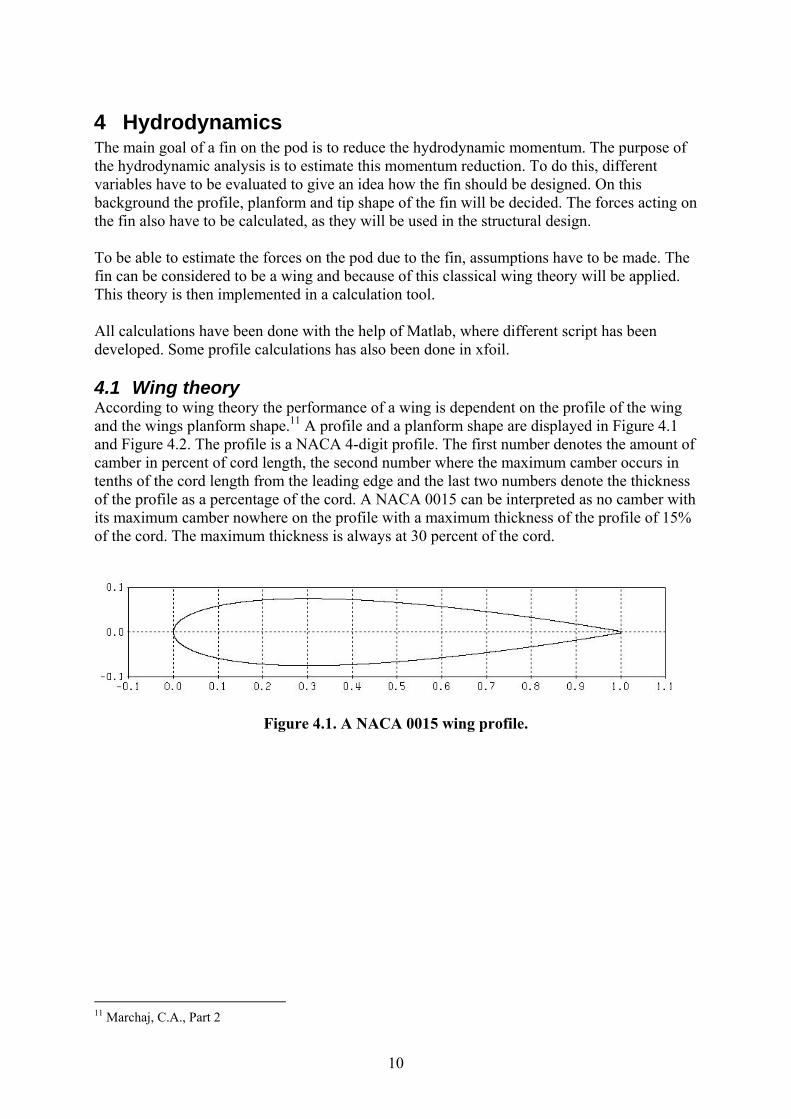
4 Hydrodynamics The main goal of a fin on the pod is to reduce the hydrodynamic momentum. The purpose of the hydrodynamic analysis is to estimate this momentum reduction. To do this, different variables have to be evaluated to give an idea how the fin should be designed. On this background the profile, planform and tip shape of the fin will be decided. The forces acting on the fin also have to be calculated, as they will be used in the structural design. To be able to estimate the forces on the pod due to the fin, assumptions have to be made. The fin can be considered to be a wing and because of this classical wing theory will be applied. This theory is then implemented in a calculation tool. All calculations have been done with the help of Matlab, where different script has been developed. Some profile calculations has also been done in xfoil. 4.1 Wing theory According to wing theory the performance of a wing is dependent on the profile of the wing and the wings planform shape.11 A profile and a planform shape are displayed in Figure 4.1 and Figure 4.2. The profile is a NACA 4-digit profile. The first number denotes the amount of camber in percent of cord length, the second number where the maximum camber occurs in tenths of the cord length from the leading edge and the last two numbers denote the thickness of the profile as a percentage of the cord. A NACA 0015 can be interpreted as no camber with its maximum camber nowhere on the profile with a maximum thickness of the profile of 15% of the cord. The maximum thickness is always at 30 percent of the cord.

Figure 4.1. A NACA 0015 wing profile.

11 Marchaj, C.A., Part 2

11

CT

CR

S

Figure 4.2. Planform, CR is the root cord, CT is the tip cord and S is the length of the fin. The forces evaluated on a wing are lift, L, and drag, D. These forces arise due to the freestream velocity, U, and the angle of attack, α. The angle of attack is the angle between the freestream and the cord line of the profile. Lift and drag are defined respectively as the force perpendicular and parallel to the freestream. 12 The mentioned quantities are shown in Figure 4.3.

Figure 4.3. U is the freestream velocity, α the angle of attack, L the lift and D the drag.

4.1.1 Wing profile When choosing a wing profile one thing among others is to decide which thickness it should have and if it should be cambered. Cambered or not is the same as choosing between a symmetric or non-symmetric profile. Only symmetric profiles are considered here due to the vast amount of options that it would give to have an unsymmetrical profile. The thickness will effect the drag and the lift-characteristics. The NACA 4-digit series will be used. This series has good stall characteristics and a good lift to drag ratio. There are other profiles that can offer lower drag at zero angle of attack but they usually have higher drag at an angle of attack.13 A good quality of the profile is that the centre of pressure does not change very much along a large speed range. Furthermore the 4-digit NACA series has a good and easy equation to generate symmetrical profiles of different thickness.

12 Marchaj, C.A., Part 2 13 www.vacantisw.com

U

L

D

α

12

To further reduce the variables on the fin it will have the same profile all along the span. Thicker profiles in general generate more drag and more lift than thinner ones, it also has a smother lift loss when it stalls. This is however very dependant of the Reynolds number. The Reynolds number indicates if the flow is laminar or turbulent. A factor not included in this number is how smooth the surface is. A rough surface triggers turbulent flow earlier than a smooth. The NACA 4-digit series is however not very sensitive to the roughness and that is why it is not regarded in this work.14

4.1.2 Wing planform The planform shape of the wing has effects on the drag. This drag arises because off a vortex created at the wingtip due to the difference in pressure on the two sides of the wing and is called induced drag. The optimal shape when minimising the vortex strength is one that gives a lift distribution along the fin that is elliptical. This distribution appears when the planform has an elliptic shape, Figure 4.4(a). A planform with a trapezoid shape, Figure 4.4(b), can be considered elliptically loaded at a tip to root cord ratio between 0.3-0.5. There is also the option to have different tapers along the length of the fin, Figure 4.4(c). The disadvantage with the elliptic planform is a more complicated manufacturing. The trapezoid shape probably is the easiest shape to manufacture of those in Figure 4.4. Another option is to have a completely rectangular planform; maybe the easiest to manufacture but it has a stronger tip vortex i.e. a higher induced drag than the other ones.15

(a) (c)(b)

Figure 4.4. (a) Elliptic planform, (b) Trapezoid planform, (c) Double tapered planform.

The planform can also be swept. This is when the fin has an angle against the body, see Figure 4.5. Sweep can somewhat change the lift distribution and in that way reduce the tip vortex. A wing that has a bigger sweep angle acts like a wing with more taper and a smaller sweep angle is equal to less taper.16

14 Abbot, I., chapter 6:4 15 Marchaj, C.A., Part 2 16 Marchaj, C.A., Part 2

13

Sweepangle

Figure 4.5. Sweep angle.

4.1.3 Wing tip shape The tip of the wing effects the induced drag. If the tip shape makes it hard for the flow to pass from the pressure to the suction side of the fin, it will have a weaker tip vortex than a shape that makes it easy. The tip can have an edge, be cut off, be rounded or fitted with an endplate or winglets, Figure 4.6. The difference between winglets and an endplate is that winglets are profile shaped and an endplate only is a plate attached to the end of the wing. Of the mentioned kinds of tips the round tip gives the strongest vortex i.e. most induced drag and the winglets or endplate probably the weakest induced drag but with an increase in frictional drag. The theory used here can not evaluate the winglet or endplate solutions in a sufficient way which leaves us to the choice off a sharp edge or a cut off edge. The cut of or square tip is preferred due to ease of manufacturing. It is also recommended for naval applications in the literature17

Thickness of the fin

Figure 4.6. Tip shapes seen from behind. Left to right: sharp edge, cut off, rounded edge

and an edge fitted with an endplate.

17 Rawson, K.J., Tupper, E.C., chap: 13

14

4.2 Forces on fin To evaluate the performance of the fin, i.e. lift and drag, first of all the profile of the fin is evaluated. This can be done with xfoil.18 Xfoil is capable of making estimations on wing profiles both for viscous and inviscid environments. This estimation is done for a 2 dimensional wing profile see Figure 4.1. Xfoil calculates the lift and drag coefficients, cl and cd, for the profile. This is then compared to linear theory. According to linear theory the 2-dimensional lift coefficient for an arbitrary profile can be expressed as19

2180lc ππα= ⋅ (4-1)

where α is the angle of attack in degrees. This equation is linear and is only valid up to the stall angle. It will be referd to as 2πα in the figures 4.7 and 4.8. An interesting thing to compare is the difference in the estimated lift-coefficient used in the calculations, according to equation (4-1), and the ones calculated by xfoil. Xfoil takes the speed into account and the lift coefficient at different speeds is shown in Figure 4.7 next to the linear estimation. Here a NACA 0015 profile is compared to the linear estimate. It is seen that the estimation is quite good between ±15°.

Figure 4.7. Comparison of the lift coefficient at different speed calculated with xfoil and

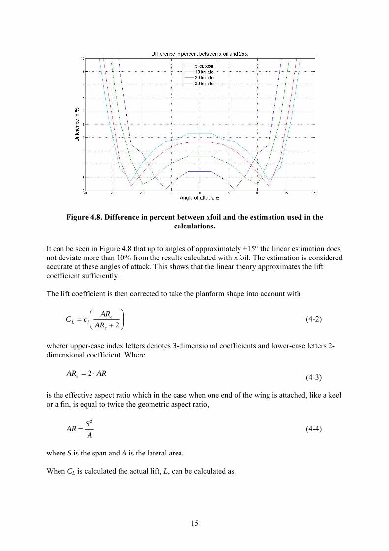
the estimation used in the calculations. The difference in percent between xfoil and the estimation is shown in Figure 4.8.

18 Drela, M., xfoil 19 Marchaj, C.A., Part 2

15

Figure 4.8. Difference in percent between xfoil and the estimation used in the

calculations.

It can be seen in Figure 4.8 that up to angles of approximately ±15° the linear estimation does not deviate more than 10% from the results calculated with xfoil. The estimation is considered accurate at these angles of attack. This shows that the linear theory approximates the lift coefficient sufficiently. The lift coefficient is then corrected to take the planform shape into account with

⎟⎟⎠

⎞⎜⎜⎝

⎛+

=2e

elL AR

ARcC (4-2)

wherer upper-case index letters denotes 3-dimensional coefficients and lower-case letters 2-dimensional coefficient. Where

ARARe ⋅= 2 (4-3) is the effective aspect ratio which in the case when one end of the wing is attached, like a keel or a fin, is equal to twice the geometric aspect ratio,

2SAR

A= (4-4)

where S is the span and A is the lateral area. When CL is calculated the actual lift, L, can be calculated as

16

212 LL V A Cρ= ⋅ (4-5)

here ρ is the density of the fluid and V is the velocity. CL, the lift coefficient, is also used when calculating the induced drag coefficient. The induced drag coefficient is defined by

2L

Die

CCAR eπ

=⋅

(4-6)

where e is the effectiveness of the planform. On an elliptically loaded wing e is 1 on other planforms e is somewhere between 0.8 and 0.9.

To be able to calculate the total drag, a total drag coefficient has to be calculated. This coefficient has two main parts, the previously mentioned induced drag and the profile drag. The profile drag consists of two components, friction drag and pressure drag. The profile drag coefficient, cd, is calculated with x-foil. The total drag coefficient is given by

DidD CcC += (4-7) The total drag can then be calculate through

212 DD V A Cρ= ⋅ (4-9)

Note that the coefficients are dependent of the angle of attack and the flow speed. This means that at different speeds and angles different profiles, planforms etc can be favourable. The choice can then be either the optimal for one condition or the best compromise to all conditions.20 The acting point of lift and drag is assumed to be at one quarter of the cord length from the leading edge. Calculations have been made in accordance with Basic Ship Theory.21 These calculations showed that the pressure acting point did only differ 0.3 percent around the assumed point. To calculate the total lift and drag on the fin, blade element theory (BET) is used. In BET the wing is divided into elements, along the span, which makes it possible to evaluate planforms with varying cord. The different elements are assumed to be independent of each other. Calculations for lift and drag is done for every segment and then added together and compensation for losses due to 3 dimensional effects as previously shown in equations (4-2)-(4-9) are made. 4.3 Forces on pod When the lift, drag and the acting point of the lift and drag are known, the momentum, MZ, and forces, Fx and Fy induced on the pod by the fin can be calculated, see Figure 3.2 for definitions. 20 Marchaj, C.A., Part 2 21 Rawson, K.J., Tupper, E.C., chap: 13

17

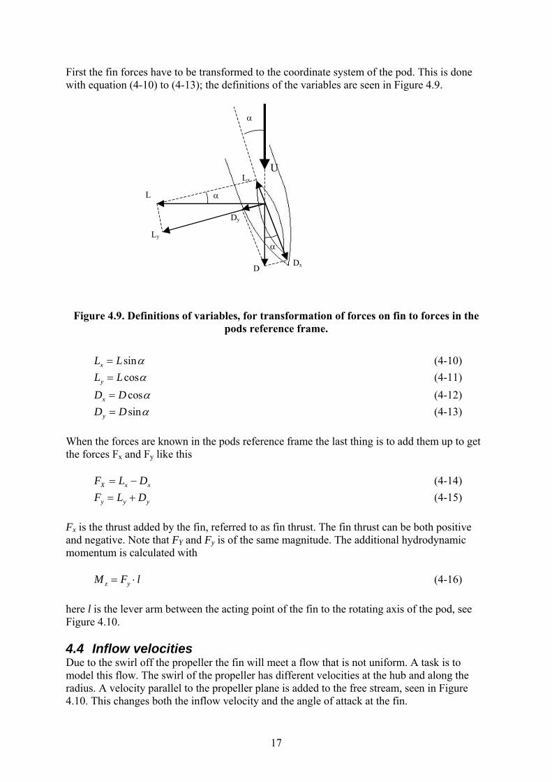
First the fin forces have to be transformed to the coordinate system of the pod. This is done with equation (4-10) to (4-13); the definitions of the variables are seen in Figure 4.9.

L

D

α

α

α

Dx

Dy

Ly

Lx

U

Figure 4.9. Definitions of variables, for transformation of forces on fin to forces in the

pods reference frame.

sinxL L α= (4-10) cosyL L α= (4-11) cosxD D α= (4-12) sinyD D α= (4-13)

When the forces are known in the pods reference frame the last thing is to add them up to get the forces Fx and Fy like this X x xF L D= − (4-14) y y yF L D= + (4-15) Fx is the thrust added by the fin, referred to as fin thrust. The fin thrust can be both positive and negative. Note that FY and Fy is of the same magnitude. The additional hydrodynamic momentum is calculated with z yM F l= ⋅ (4-16)

here l is the lever arm between the acting point of the fin to the rotating axis of the pod, see Figure 4.10. 4.4 Inflow velocities Due to the swirl off the propeller the fin will meet a flow that is not uniform. A task is to model this flow. The swirl of the propeller has different velocities at the hub and along the radius. A velocity parallel to the propeller plane is added to the free stream, seen in Figure 4.10. This changes both the inflow velocity and the angle of attack at the fin.

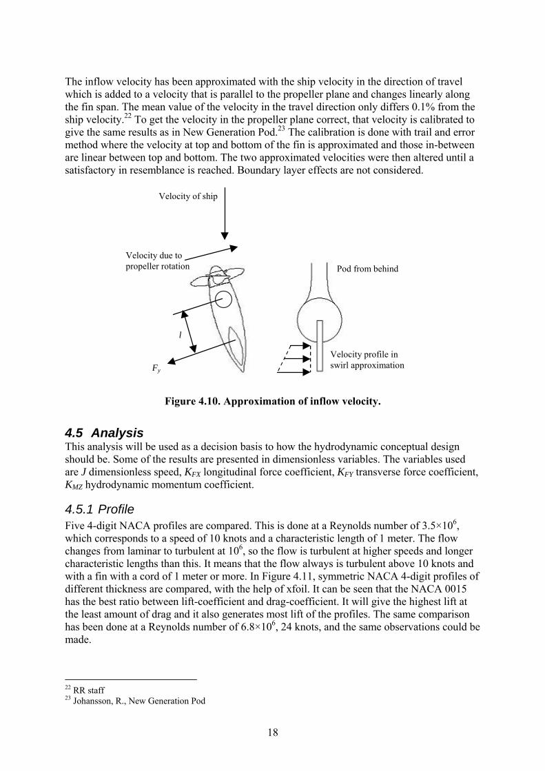
18

The inflow velocity has been approximated with the ship velocity in the direction of travel which is added to a velocity that is parallel to the propeller plane and changes linearly along the fin span. The mean value of the velocity in the travel direction only differs 0.1% from the ship velocity.22 To get the velocity in the propeller plane correct, that velocity is calibrated to give the same results as in New Generation Pod.23 The calibration is done with trail and error method where the velocity at top and bottom of the fin is approximated and those in-between are linear between top and bottom. The two approximated velocities were then altered until a satisfactory in resemblance is reached. Boundary layer effects are not considered.

Velocity of ship

Velocity profile inswirl approximation

Velocity due topropeller rotation Pod from behind

l

Fy

Figure 4.10. Approximation of inflow velocity.

4.5 Analysis This analysis will be used as a decision basis to how the hydrodynamic conceptual design should be. Some of the results are presented in dimensionless variables. The variables used are J dimensionless speed, KFX longitudinal force coefficient, KFY transverse force coefficient, KMZ hydrodynamic momentum coefficient.

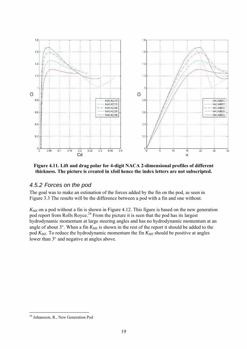
4.5.1 Profile Five 4-digit NACA profiles are compared. This is done at a Reynolds number of 3.5×106, which corresponds to a speed of 10 knots and a characteristic length of 1 meter. The flow changes from laminar to turbulent at 106, so the flow is turbulent at higher speeds and longer characteristic lengths than this. It means that the flow always is turbulent above 10 knots and with a fin with a cord of 1 meter or more. In Figure 4.11, symmetric NACA 4-digit profiles of different thickness are compared, with the help of xfoil. It can be seen that the NACA 0015 has the best ratio between lift-coefficient and drag-coefficient. It will give the highest lift at the least amount of drag and it also generates most lift of the profiles. The same comparison has been done at a Reynolds number of 6.8×106, 24 knots, and the same observations could be made.

22 RR staff 23 Johansson, R., New Generation Pod

19

Figure 4.11. Lift and drag polar for 4-digit NACA 2-dimensional profiles of different thickness. The picture is created in xfoil hence the index letters are not subscripted.

4.5.2 Forces on the pod The goal was to make an estimation of the forces added by the fin on the pod, as seen in Figure 3.3 The results will be the difference between a pod with a fin and one without. KMZ on a pod without a fin is shown in Figure 4.12. This figure is based on the new generation pod report from Rolls Royce.24 From the picture it is seen that the pod has its largest hydrodynamic momentum at large steering angles and has no hydrodynamic momentum at an angle of about 3°. When a fin KMZ is shown in the rest of the report it should be added to the pod KMZ. To reduce the hydrodynamic momentum the fin KMZ should be positive at angles lower than 3° and negative at angles above.

24 Johansson, R., New Generation Pod

20

Figure 4.12. KMZ for a pod without a fin, measured by Rolls Royce.

To get a descent result of the propeller swirl it has been calibrated and compared with the results in the report New Generation Pod.25 These tests were run at a speed of 24 kn, propeller diameter of 4.7m and a propeller rotational speed of 164 rpm. The calibrated velocity profile, done as mentioned before, that made the best resemblance is used in the calculations. Focus has been set on making the approximation of the difference in Mz as good as possible, because this is the variable to reduce. The best approximation is shown in Figure 4.13.

Figure 4.13. Difference in KMz calculated with the used model compared to those

measured by Rolls Royce in cavitation tunnel tests.

25 Johansson, R., New Generation Pod

21

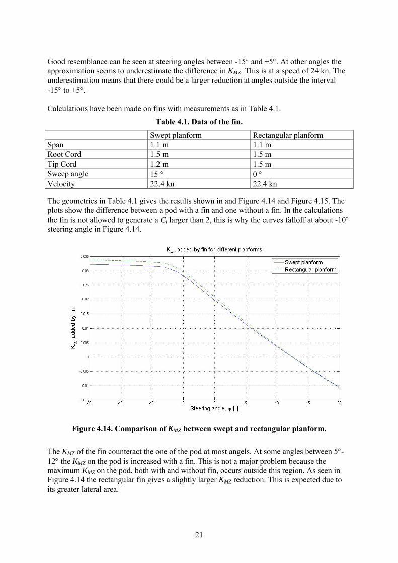
Good resemblance can be seen at steering angles between -15° and +5°. At other angles the approximation seems to underestimate the difference in KMZ. This is at a speed of 24 kn. The underestimation means that there could be a larger reduction at angles outside the interval -15° to +5°. Calculations have been made on fins with measurements as in Table 4.1.

Table 4.1. Data of the fin.

Swept planform Rectangular planform Span 1.1 m 1.1 m Root Cord 1.5 m 1.5 m Tip Cord 1.2 m 1.5 m Sweep angle 15 ° 0 ° Velocity 22.4 kn 22.4 kn The geometries in Table 4.1 gives the results shown in and Figure 4.14 and Figure 4.15. The plots show the difference between a pod with a fin and one without a fin. In the calculations the fin is not allowed to generate a Cl larger than 2, this is why the curves falloff at about -10° steering angle in Figure 4.14.

Figure 4.14. Comparison of KMZ between swept and rectangular planform.

The KMZ of the fin counteract the one of the pod at most angels. At some angles between 5°-12° the KMZ on the pod is increased with a fin. This is not a major problem because the maximum KMZ on the pod, both with and without fin, occurs outside this region. As seen in Figure 4.14 the rectangular fin gives a slightly larger KMZ reduction. This is expected due to its greater lateral area.

22

At its most the momentum added by the fin is about 450 kNm. A pod of the size that fits the fin will at its most produce a torque of about 900 kNm.26 This implies that the azimuth torque can be reduced to half. These numbers are calculated at service speed of the pod, 22.4 kn. It is not probable that the hydrodynamic momentum has the same relative behaviour at other speeds. This is because the swirl is approximated at one speed. At other speeds the swirl probably has another relation to the free stream. If this model is used at lower speeds it will probably overestimate the momentum reduction due to the fact that the lift varies with the square of the speed. If it is used at higher speeds it will probably underestimate the momentum. It is hard to conclude which relations the free stream and the swirl have to each other with only one measured speed as background. The force along the pod, fin thrust, changes with the steering angle as shown in Figure 4.15.

Figure 4.15. Comparison of KFX between swept and rectangular planform.

It is seen in Figure 4.15 that at some angles there is some resistance. The largest resisting force is about 700 N and occurs at a steering angle of 12°. At a speed of 22.4 knots this represents a power of about 8 kW; this is negligible in comparison to the 10 MW power of the pod. At straightforward condition a small positive fin thrust is achieved. This increase is about 5kN, which is equal to a power of 57 kW and a thrust increase of about 0.5%. As mentioned in the profile section the linear approximation cannot be considered accurate outside steering angles of ±15°. It is seen in these comparisons that a rectangular fin with larger area gives a larger reduction in hydrodynamic momentum and a bigger force in the length direction of the pod. A Matlab code that computes the cord of a rectangular fin where the fin thrust is zero is developed. with the help of this you can predict if the fin will give positive or negative fin thrust. A longer cord gives a larger lift force but also larger friction and induced drag. Depending on the angle of attack, different cord lengths where the fin thrust is zero. The lift

26 RR staff

23

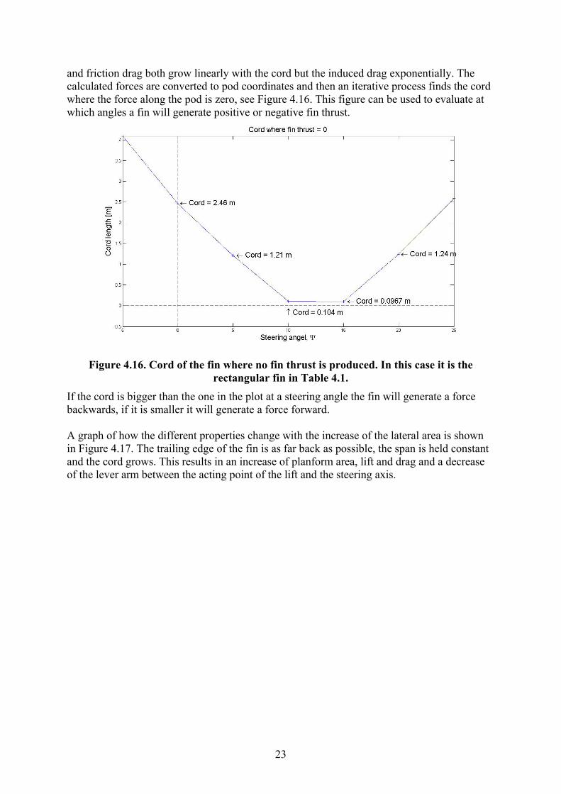
and friction drag both grow linearly with the cord but the induced drag exponentially. The calculated forces are converted to pod coordinates and then an iterative process finds the cord where the force along the pod is zero, see Figure 4.16. This figure can be used to evaluate at which angles a fin will generate positive or negative fin thrust.

Figure 4.16. Cord of the fin where no fin thrust is produced. In this case it is the

rectangular fin in Table 4.1. If the cord is bigger than the one in the plot at a steering angle the fin will generate a force backwards, if it is smaller it will generate a force forward. A graph of how the different properties change with the increase of the lateral area is shown in Figure 4.17. The trailing edge of the fin is as far back as possible, the span is held constant and the cord grows. This results in an increase of planform area, lift and drag and a decrease of the lever arm between the acting point of the lift and the steering axis.

24

Figure 4.17. Graph over how the properties grow with change of area, the trailing edge of the fin is as far back as possible. The increasing line represents the lift, acting point

position and area. All quantities are normalised with its own maximum except the drag that is normalised with maximum lift for comparison reasons.

Here it is seen that the momentum Mz has a maximum when the fin has its lift acting point at a distance that is half way between the trailing edge and the steering axis. If the fin should have its acting point in front of this distance the momentum, Mz, decreases but the drag increases. The drag curve suggests that the fin should be as short as possible. The drag is normalised with the lift to visualise the difference in size of these two. This plot implies that the fin should be equal to or shorter than half the distance from the trailing edge to the steering axis.

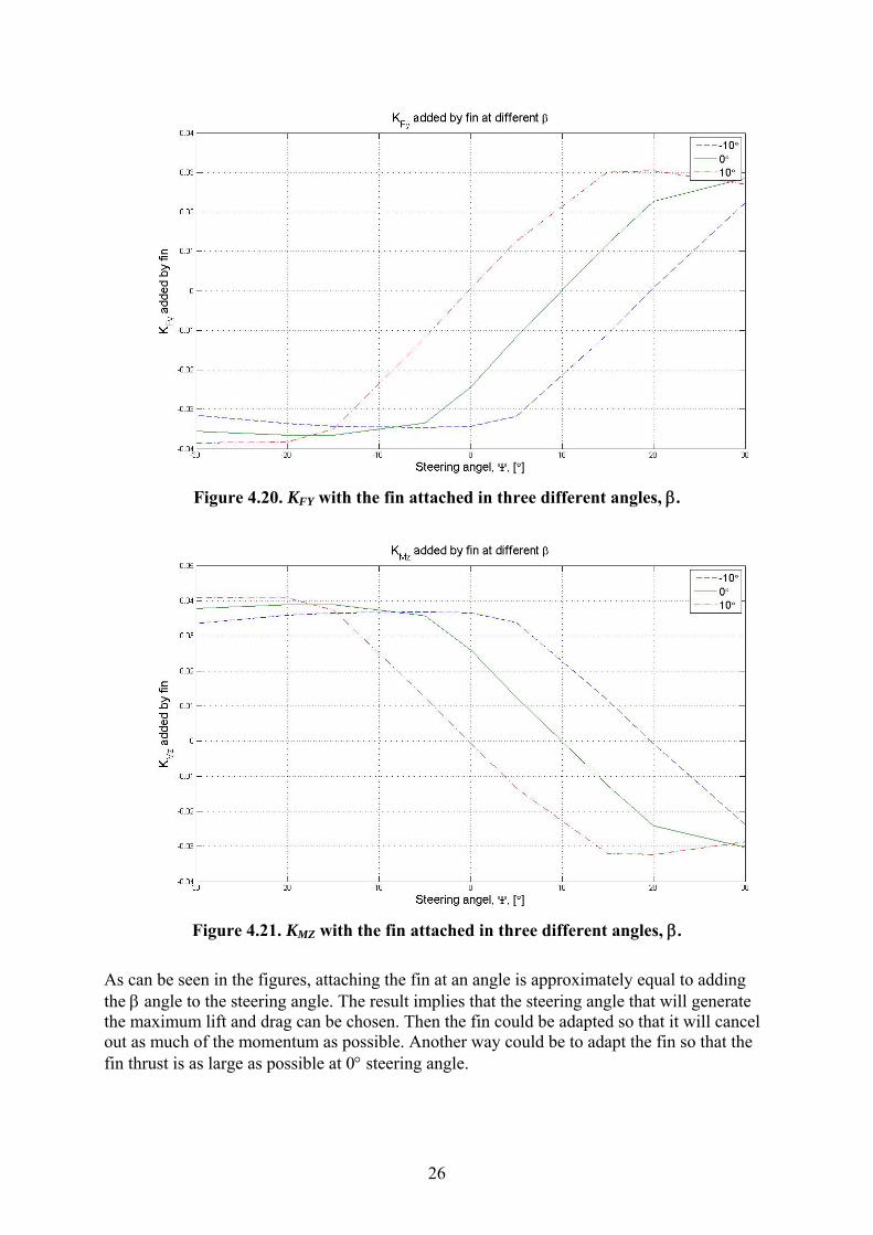
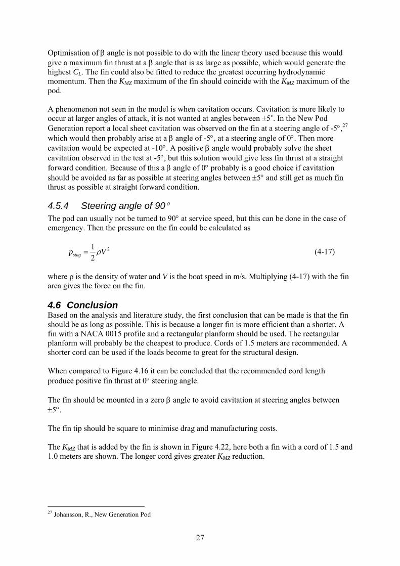
4.5.3 Fin attached at an angle to the pod The fin can be attached at an angle to the pod to try to optimise the efficiency. The definition of β, the angle at which the fin is attached, is shown in Figure 4.18. Different fin angles have been compared in Figure 4.19, Figure 4.20 and Figure 4.21.

25

Figure 4.18. Definition of β angle when fin attached to pod

Figure 4.19. KFX with the fin attached in three different angles, β.

β - +

26

Figure 4.20. KFY with the fin attached in three different angles, β.

Figure 4.21. KMZ with the fin attached in three different angles, β.

As can be seen in the figures, attaching the fin at an angle is approximately equal to adding the β angle to the steering angle. The result implies that the steering angle that will generate the maximum lift and drag can be chosen. Then the fin could be adapted so that it will cancel out as much of the momentum as possible. Another way could be to adapt the fin so that the fin thrust is as large as possible at 0° steering angle.

27

Optimisation of β angle is not possible to do with the linear theory used because this would give a maximum fin thrust at a β angle that is as large as possible, which would generate the highest CL. The fin could also be fitted to reduce the greatest occurring hydrodynamic momentum. Then the KMZ maximum of the fin should coincide with the KMZ maximum of the pod. A phenomenon not seen in the model is when cavitation occurs. Cavitation is more likely to occur at larger angles of attack, it is not wanted at angles between ±5˚. In the New Pod Generation report a local sheet cavitation was observed on the fin at a steering angle of -5°,27 which would then probably arise at a β angle of -5°, at a steering angle of 0°. Then more cavitation would be expected at -10°. A positive β angle would probably solve the sheet cavitation observed in the test at -5°, but this solution would give less fin thrust at a straight forward condition. Because of this a β angle of 0° probably is a good choice if cavitation should be avoided as far as possible at steering angles between ±5° and still get as much fin thrust as possible at straight forward condition.

4.5.4 Steering angle of 90° The pod can usually not be turned to 90° at service speed, but this can be done in the case of emergency. Then the pressure on the fin could be calculated as

212stagp Vρ= (4-17)

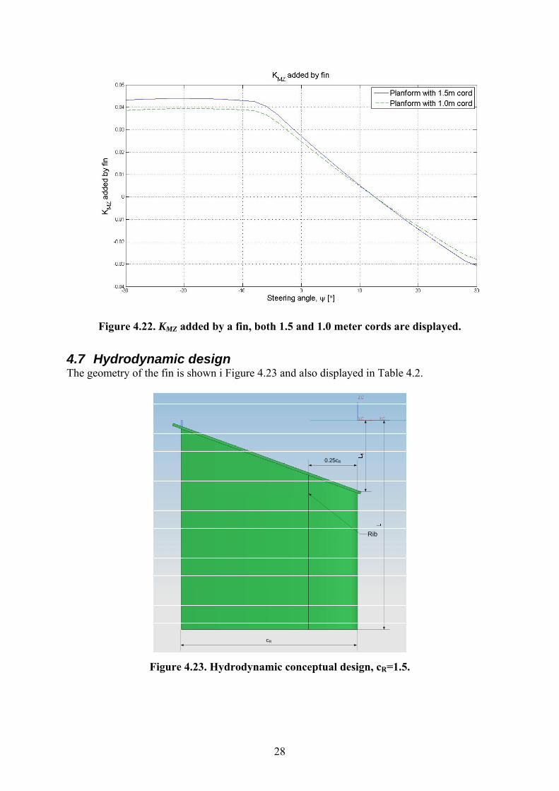
where ρ is the density of water and V is the boat speed in m/s. Multiplying (4-17) with the fin area gives the force on the fin. 4.6 Conclusion Based on the analysis and literature study, the first conclusion that can be made is that the fin should be as long as possible. This is because a longer fin is more efficient than a shorter. A fin with a NACA 0015 profile and a rectangular planform should be used. The rectangular planform will probably be the cheapest to produce. Cords of 1.5 meters are recommended. A shorter cord can be used if the loads become to great for the structural design. When compared to Figure 4.16 it can be concluded that the recommended cord length produce positive fin thrust at 0° steering angle. The fin should be mounted in a zero β angle to avoid cavitation at steering angles between ±5°. The fin tip should be square to minimise drag and manufacturing costs. The KMZ that is added by the fin is shown in Figure 4.22, here both a fin with a cord of 1.5 and 1.0 meters are shown. The longer cord gives greater KMZ reduction.

27 Johansson, R., New Generation Pod

28

Figure 4.22. KMZ added by a fin, both 1.5 and 1.0 meter cords are displayed.

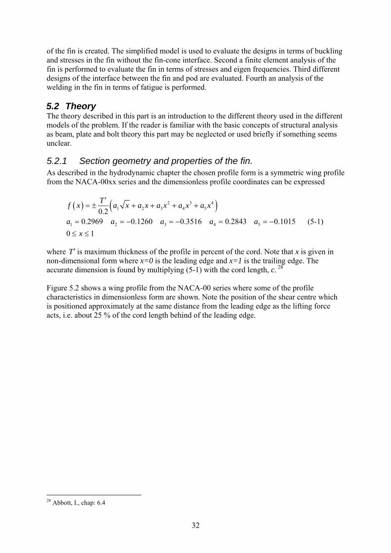
4.7 Hydrodynamic design The geometry of the fin is shown i Figure 4.23 and also displayed in Table 4.2.

Rib

cR

0.25cR

Figure 4.23. Hydrodynamic conceptual design, cR=1.5.

29

Table 4.2. Geometrial propeteris of the fin.

Quantity Abbreviation Value Design 1

Value Design 2

Unit

Cord cR 1.5 1.0 m Length L 1.7 1.7 m Difference in length between leading and trailing edge

L1 0.6 0.4 m

Forces on the fin with two different cords used in the structural analysis are shown in Table 4.3. Loading condition for fatigue analysis is shown in Table 4.4.

Table 4.3. Loading condition for the two designs.

Quantity Abbreviation Value Design 1

Value Design 2

Unit

Force from stagnation pressure Fstag 135 96 kN Force lateral Fy 108 84 kN Force longitudinal Fx 29 30 kN

Table 4.4. Loading condition for fatigue analysis of design 1.

Quantity Abbreviation UnitSteering angle ψ +35˚ +15˚ +5˚ +2˚ -2˚ -5˚ -15˚ -35˚ deg Force lateral Fy -102 -108 -90 -72 -47 -29 29 79 kN 4.8 Future work To take the hydro dynamical analysis further, CFD calculations and cavitation tunnel tests must be performed. In these tests different shapes should be evaluated, i.e. planform shape, tip shape and different and cambered profiles. In this work the focus has been set on reducing the hydrodynamic momentum and the propulsive benefits have come as a side effect. A different way could be to maximize the propulsive benefits and let the hydrodynamic momentum be the secondary objective. This could maybe be a way to improve the life time economy of a ship.

30

5 Structural Design 5.1 Introduction The fin has to resist both static and dynamic loads induced during operation. Meanwhile the strength requirements of the fin is fulfilled the construction must be simple to manufacture with efficient usage of material so the total weight is not unnecessarily high. If the fin has an unnecessarily high weight it might be difficult to handle the fin in dockings during maintenance situations. Not to mention the economic aspects where the costs should be kept as low as possible. Two designs have been considered in the hydrodynamic chapter the details are found in Figure 4.23 and Table 4.2, but for a general view see Figure 5.1. These designs are to be analyzed in terms of strength.

Fin foot

Fin

Figure 5.1. Model of the fin created in NX with long foot.

In addition to the general structural layout the designs have to fulfil the regulations from the classification societies. The two designs have also been based on the DNV classification society rules and guidelines in terms of material thicknesses. Governing DNV criteria is in all cases the shell minimum thickness. These may be found in Table 5.1

Table 5.1. DNV regulations for dimensions of a rudder (fin).

Quantity Abbreviation Value Design 1

Value Design 2

Unit

Shell thickness ts 22 17 mm Web thickness tw 16 12 mm Frame thickness tf 16 12 mm

Each design have also been analysed with a long and a short foot. In the case with short foot, the foot starts at the leading edge of the fin and have a length of approximate half the cord length at the root.

31

The construction is made of welded plates, with a longitudinal web, a foot and bottom plating, with a shell swept around. This means that the fin can be considered as a thin-wall stiffened structure. The fin foot and the bottom plating on the fin acts like frames and contribute to maintain the shape of the profile. The web maintains the shape of the profile but also carries shear forces acting in the beam. The interface between the fin and the pod is assumed to be a ordinary bolt connection. It is assumed that the fin is manufactured with both plane and single curved plates which then are welded together. The forces acting on the fin can be found in Table 4.3 and Table 4.4. There are three main loading conditions to be considered.

1. Service speed condition with or without steering angle applied. This condition is highly dynamic due to the propeller slip stream and fatigue analysis is to be done.

2. Crash stop condition. This is a condition where the worst case is when the pod is perpendicular to the centre line. The speed at this condition is lower than the ordinary service speed but may be overridden in times of emergency.

3. Direct impact for e.g. grounding. In this case the fin should fall of before any other part of the pod is damaged.

The two first loading conditions are found in the hydrodynamic chapter. The third has to be examined through an iterative process where the impact force is increased until something is damaged. The forces acting on the fin are recalculated to a pressure load which is acting on the area of one side of the fin. This is not correct but the assumption simplifies the load case a lot.The consequences in spanwise direction are that the stresses in the fin will be greater than if the correct load distribution is used which indicates that it is a conservative assumption. In the cordwise direction it is a quite rough approximation which probably is not suitable for a detail study of the structure. However for a global analysis of the stress, this seems like a reasonable assumption. For this study a common steel alloy will be used. It seems reasonable to use a similar steel alloy as in the pod itself. By this assumption tabulated properties for the steel is available. In Table 5.2 below the properties, of the steel alloy applied in the study, are listed.

Table 5.2. Physical properties of the steel applied in the present study.

Quantity Abbreviation Value Unit Density ρ 7850 kg/m3 Young's modulus E 208 GPa Poisson's ratio ν 0.3 - Ultimate strength σcr 360-460 MPa Yield strength σy 260 MPa Yield Shear strength τsv 140 MPa Fatigue strength (puls) σubp 150±150 MPa Fatigue strength σub 170 MPa Fatigue shear strength τubp 100±100 MPa

In the following chapter, a part with theory will follow which briefly describes the governing relations between material- and geometric properties. Then an analysis of the structural problem will follow. The analysis is divided into several parts. First a simplified beam model

32

of the fin is created. The simplified model is used to evaluate the designs in terms of buckling and stresses in the fin without the fin-cone interface. Second a finite element analysis of the fin is performed to evaluate the fin in terms of stresses and eigen frequencies. Third different designs of the interface between the fin and pod are evaluated. Fourth an analysis of the welding in the fin in terms of fatigue is performed. 5.2 Theory The theory described in this part is an introduction to the different theory used in the different models of the problem. If the reader is familiar with the basic concepts of structural analysis as beam, plate and bolt theory this part may be neglected or used briefly if something seems unclear.

5.2.1 Section geometry and properties of the fin. As described in the hydrodynamic chapter the chosen profile form is a symmetric wing profile from the NACA-00xx series and the dimensionless profile coordinates can be expressed

( ) ( )2 3 41 2 3 4 5

1 2 3 4 5

0.20.2969 0.1260 0.3516 0.2843 0.1015

0 1

Tf x a x a x a x a x a x

a a a a ax

′= ± + + + +

= = − = − = = −≤ ≤

(5-1)

where T ′ is maximum thickness of the profile in percent of the cord. Note that x is given in non-dimensional form where x=0 is the leading edge and x=1 is the trailing edge. The accurate dimension is found by multiplying (5-1) with the cord length, c. 28 Figure 5.2 shows a wing profile from the NACA-00 series where some of the profile characteristics in dimensionless form are shown. Note the position of the shear centre which is positioned approximately at the same distance from the leading edge as the lifting force acts, i.e. about 25 % of the cord length behind of the leading edge.

28 Abbott, I., chap: 6.4

33

0 0.2 0.4 0.6 0.8 1

-0.3

-0.2

-0.1

0

0.1

0.2

0.3

NACA - 0015; Ixx/c3ts= 0.0062452

x [-]

f(x)

[-]

Profile shellCentre of gravity xcg/c= 0.49021

Shear centre ξs/c= 0.25797

Figure 5.2. Thin wall wing profile from the NACA-00 series. Properties of the profile

shell are given in non-dimensional form. The shell centre of gravity can be calculated as follows, assuming that the shell thickness is the same around the whole profile,

( )( )

2

2

1

1

x f x dxx

f x dx

′+=

′+

∫∫

(5-2)

which is a method of moment equivalence.29 Due to symmetry the centre of gravity around the x-axis is zero, hence is 0y = . The moment of inertia for a shell with respect to a point can be calculated as

( ) ( ) ( )2 2 22, ,1 1xx O s yy O sI f x t f x dx I x t f x dx′ ′= + = +∫ ∫ (5-3)

where ts is the thickness of the shell.30 If the moment of inertia is not calculated with respect to the centre of gravity this has to be compensated for according to Steiner's rule.31 The coordinate system has the origin, O, at the leading edge and therefore the moment of inertia of the y-axis has to be moved to the centre of gravity. The Steiner contribution is applied as

29 Sundström B., chap: 31.1 in combination with Råde, B., Westergren, L., chap: 7.3 30 Råde, B., Westergren, L., chap: 7.3 31 Sundström, B., chap: 31.1.1

34

2

,

,

yy yy O

xx xx O

I I x A

I I

= −

= (5-4)

The coupling moment of inertia, Ixy, is zero, due to symmetry around the x-axis. The shear centre is the point the section twists about when a shear load, S, is applied. The shear centre can be found by using the method of moment equivalence. Since a load that is not acting through the shear centre creates a moment which corresponds with the moment created by the shear flow, q, it is possible to determine the shear centre. The shear flow is produced by the applied shear force and may be calculated as follows.32

,02 20 0

s sx xx y xy y yy x xy

s s s sxx yy xy xx yy xy

S I S I S I S Iq t xds t yds q

I I I I I I⎛ ⎞ ⎛ ⎞− −

= − − +⎜ ⎟ ⎜ ⎟⎜ ⎟ ⎜ ⎟− −⎝ ⎠ ⎝ ⎠∫ ∫ (5-5)

( )

,0

/

/b s

ss

q Gt dsq

ds Gt= − ∫

∫ (5-6)

where qs is the shear flow, qb is the base shear flow, qs0 is the initial shear flow, s is the coordinate along the profile in natural coordinates and G is the shear modulus. Index at S indicates which direction the shear acts in. The moment equivalence can the be expressed as i i s

i

S L q lds=∑ ∫ (5-7)

where L is the lever arm from the shear load to the shear centre and l is the local lever arm for qs acting on ds.33 When applying a load which does not act through the shear centre a torsional moment is created. Hence the section's torsion properties must be taken into account. For a closed section the torsion can, according to Bredt-Batho formulas34, be expressed as

24v

s

d M dsdz A Gtθ= ∫ (5-8)

where A is the enclosed area of the profile and can due to symmetry be calculated as ( )2A f x dx= ∫ (5-9)

further

32 Megson T.H.G., chap: 9.4.2 33 Megson T.H.G., chap: 9.4 34 Megson T.H.G., chap: 9.5.1.

35

( )22 1ds f x dx′= +∫ ∫ (5-10)

is the total length of the profile arc due to symmetry. Finally Mv is the twisting moment produced by force not acting through the shear centre.

5.2.2 Beam theory The governing equation for a beam subjected to a distributed load can be expressed as

( ) ( )2 2

2 2d d wEI x q xdx dx

⎡ ⎤=⎢ ⎥

⎣ ⎦ (5-11)

where w denotes the deflection, q is the distributed load and E is Young's modulus of the construction material. Note that (5-11) allows the moment of inertia to vary along the length of the beam.35 Further the shear forces, T, and bending moment, M, can be calculated from the following expressions

( ) ( )

( ) ( )

dT xq x

dxdM x

T xdx

= −

=

(5-12)

which are the equilibrium equations of a beam element.36 The direct stresses in a beam can be calculated as

( )( )

( )( )

N x M xz

A x I xσ = + (5-13)

and the average shear stress as

TA

τ μ= (5-14)

where μ is a characteristic parameter for the section which can be found in standard textbooks for solid mechanics.37

5.2.3 Plate theory The governing differential equation for a plate subjected to transverse and in-plane loads, as in Figure 5.3, may be written as

35 Sundström, B, chap: 6.2.2.5. 36 Sundström, B., chap: 6.2.2.1. 37 Sundström, B, chap: 6.2.2.3-4

36

2

2 2 2

2 2 2x y xy

D w qw w wq q N N N

x y x y

∗

∗

Δ =

∂ ∂ ∂= + + +

∂ ∂ ∂ ∂

(5-15)

where q is a lateral pressure, N is in-plane loads, D is the flexural rigidity, w is the transverse deflection and Δ is the Laplace operator.38

Figure 5.3. Characteristics of the plate.

Solutions to the plate equation are often gained by the usage of trigonometric series,and tabulated formulas for deflection and moments are available for different aspect ratios, a/b, and boundary conditions.39 The critical buckling load for a simply supported plate, subjected to an in-plane load along the plate's shortest side, can be written as

2

2

2

crDP K

b

mb aKa mb

π=

⎡ ⎤⎛ ⎞ ⎛ ⎞= +⎜ ⎟ ⎜ ⎟⎢ ⎥⎝ ⎠ ⎝ ⎠⎣ ⎦

(5-16)

where m describes the buckling mode. As seen, K, the buckling coefficient, is depending on the aspect ratio. K is also depending on the boundary condition. There are tabulated values for different boundary conditions which can be used directly into (5-16).40 The critical shear stress load for a plate can be expressed as

38 Megson, T.H.G:, chap: 9.4. 39 Young, W.C., et al chap: 11 40 Young, W.C., et al chap: 11

y

37

2

2cr sDk

b hπτ = (5-17)

where ks is the shear buckling coefficientand h the plate thickness. ks is depending on the aspect ratio and the boundary condition and may be found in various textbooks for the actual conditions.41 Stresses from in-plane loads which have the dimension [N/m] can be expressed as

Nh

σ = (5-18)

Further the stresses in the plate can generally be calculated with knowledge of the moments in the plate by using42

max 26Mh

σ = . (5-19)

The total stress in the shell is then found by adding (5-13) with (5-19).

5.2.4 Fatigue Fatigue decreases the strength of the material which implies that failure can occur at stress levels far below ultimate strength level. Fatigue is a dynamic phenomenon that can take many forms e.g. cyclic loading and corrosion. In the case where the structural member is behind the propeller where the loads are highly time dependent it seems reasonable to perform a high cyclic fatigue analysis. One simple way of fatigue analysis is to consider infinite life of the object. In addition to this no reductions, for e.g. the quality of the surface in terms defects and roughness, are done. Simple handbook tables for allowable fatigue stresses in the material are available. Something that may be treated both as high or low cycle fatigue is when the steering angle, ψ, shifts between negative and positive values. A fatigue load spectrum shows that loads at steering angles of magnitude ± 15˚ occurs 106 times during a life time. Note that for a common steel alloy the allowed stress threshold does not change for cycles above 106-107 cycles. A reasonable way of treating the fatigue design aspects is therefore to consider infinite life time of the product and use tabulated threshold values of the allowed stress.43 When using welding techniques for connecting parts that are subjected to a dynamic load a fatigue analysis of the welding is necessary. There are several methods to evaluate this phenomena e.g. by FEM calculations, simplified methods found in standard textbooks and the whole range between them. "Svenskt stål AB" (SSAB), suggests a simplified method of controlling the weld in terms of fatigue. The method is referring to the number of load cycles, type of weld, probability for 41 Huss, M., chap: 4.2.5. 42 Zenkert, D., 43 RR staff

38

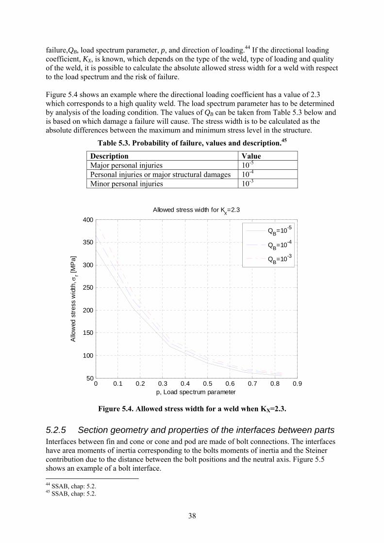
failure,QB, load spectrum parameter, p, and direction of loading.44 If the directional loading coefficient, KX, is known, which depends on the type of the weld, type of loading and quality of the weld, it is possible to calculate the absolute allowed stress width for a weld with respect to the load spectrum and the risk of failure. Figure 5.4 shows an example where the directional loading coefficient has a value of 2.3 which corresponds to a high quality weld. The load spectrum parameter has to be determined by analysis of the loading condition. The values of QB can be taken from Table 5.3 below and is based on which damage a failure will cause. The stress width is to be calculated as the absolute differences between the maximum and minimum stress level in the structure.

Table 5.3. Probability of failure, values and description.45

Description Value Major personal injuries 10-5 Personal injuries or major structural damages 10-4 Minor personal injuries 10-3

0 0.1 0.2 0.3 0.4 0.5 0.6 0.7 0.8 0.950

100

150

200

250

300

350

400

p, Load spectrum parameter

Allo

wed

stre

ss w

idth

, σr [M

Pa]

Allowed stress width for Kx=2.3

QB=10-5

QB=10-4

QB=10-3

Figure 5.4. Allowed stress width for a weld when KX=2.3.

5.2.5 Section geometry and properties of the interfaces between parts Interfaces between fin and cone or cone and pod are made of bolt connections. The interfaces have area moments of inertia corresponding to the bolts moments of inertia and the Steiner contribution due to the distance between the bolt positions and the neutral axis. Figure 5.5 shows an example of a bolt interface. 44 SSAB, chap: 5.2. 45 SSAB, chap: 5.2.

39

X

rb

x

Figure 5.5. Example of a bolt interface.

The area moment of inertia around the x-axis of a bolt can be expressed as

4

2

4b

xx brI A yπ

= + (5-20)

where rb is the bolt average radius, Ab is the bolt area and y is the distance between the bolt and the area centre of gravity of the bolts. Total moment of inertia is gained by summing up the contributions from all the bolts. The moment of inertia around the y-axis is calculated in a similar way.

5.2.6 Bolt connection theory The most used technique to unite parts, in a connection that is not permanent, is the usage of bolt connections. Figure 5.6 shows a bolt connection.

Figure 5.6. Principal sketch of a bolt connection.

The length of the bolt should at least be four times the diameter of the bolt. The reason for this is to secure that the bolt is weak in comparison to the flange, in this case the flange consists of the parts that should be joined. When threading the bolt directly in the flange material a depth, Lt, of at least the diameter is needed for the connection. In addition to this the threading should have some extra millimetres as a margin and the drilling hole should be 5-10 mm deeper so the threading tools have enough space.46

46 Bonde-Wiiburg, chap: 7.1.

40

Bolts are in most cases subjected to an initial load that creates stresses and therefore also an elongation, δ, in the bolt. The reason for this is to maintain the connection between the parts when an external load is applied. A scheme for this is shown in Figure 5.7.47 The initial force, F0 is applied during the joining of the parts. When the external load is applied the total bolt force, Fb is increased and the force that maintains the connection, Ff is decreased due to the force equivalence which must be fulfilled. If the bolt is weak compared to the flanges the resulting bolt force will be the in same magnitude as the initial force. The total bolt stress can, if Young's modulus is equal and the length of the bolt and flange is equal, be calculated as

01

1t L

f

b

AA

σ σ σ= ++

(5-21)

where σt is the total stress, σ0 is the initial stress, σL is the applied stress calculated as in (5-13) and Af is the effective flange area which can be calculated as

( )2 20.34f hA N L Dπ ⎡ ⎤= + −⎣ ⎦ (5-22)

where N is the key width needed for the bolt skull, L is the length of the bolt and Dh is the diameter of hole in the flange needed for the bolt.48

Figure 5.7. F-δ diagram for a bolt with external load applied.

When the bolt is subjected to a dynamic load a fatigue analysis of the bolt must be performed. The external load must not gain a bolt force over a certain threshold value or the additional

47 Bonde-Wiiburg, chap: 7.1. 48 Andersson, S., chap: 14.6.4.

41

bolt stress is not to be greater than a threshold value which may be found in standard bolt handbooks or in data sheets from the bolt manufacturer.49 Normally bolt connections are constructed so that they do not carry any shear forces through the bolts but with the friction force created between the parts, which is a consequence of the initial stress that the bolts are subjected to. If this is not enough additional shear pins are added that will take all the shear forces. The critical shear stress is calculated by (5-14) and can for circular shear elements can be expressed as

24

3T

n rτ

π= (5-23)

where n is number of shear pins, T is the shear force and r is the radius of a shear pin.

5.2.7 Numerical approximations For simplicity some of the above described equations may be evaluated with some numerical method e.g. Simpson's method. For some integrals some appropriate substitution, to avoid division by zero, may be required. The Simpson's method may be written as

( ) ( ) ( ) ( )

1

0 2 1 2 21 1

0 2

4 23

2

n n

k k nk k

n

hI f x f x f x f x

b ah a x b xn

−

−= =

⎡ ⎤≈ + + +⎢ ⎥⎣ ⎦−

= = =

∑ ∑ (5-24)

where b is the end point, a is the start point of the interval and n is number of intervals. The differential equation (5-11) is for simplicity solved with the method of finite differences. This is done by replacing the derivates of the deflections along the beam with approximate derivates as shown below

( ) ( )

( ) ( )

( ) ( )

( ) ( )

1 1

1 12

2 1 1 23

2 1 1 24

121

1 2 221 4 6 4

i i i

i i i i

i i i i i

i i i i i i

w x w wh

w x w w wh

w x w w w wh

w x w w w w wh

+ −

+ −

+ + − −

+ + − −

′ ≈ −

′′ ≈ − +

′′′ ≈ − + −

′′′′ ≈ − + − +

(5-25)

Where all approximations above are of the second order. This is used to obtain a linear system of type =Aw q (5-26) where A is the system matrix containing information about material properties, moment of inertia and the derivatives of the same, w is a vector with deflections and q is a vector 49 Colly Company AB, chap: 4.8.

42

containing the distributed force.50 The derivatives of the moment of inertia are obtained by a polynomial approximation of the moment of inertia. 5.3 Beam model

5.3.1 Introduction The main purpose with a beam model is to evaluate designs in terms of deflection, stresses and buckling and finding acceptable designs that can be investigated further. A second reason for developing a simplified model is to evaluate if, the results after a finite element calculation, seems reasonable. The fin, which has the form of a wing profile, is a thin-walled stiffened structure subjected to a pressure distribution due to the hydrodynamics in the propeller slipstream. A reasonable simplification is that the fin can be approximated with a cantilever beam, clamped-free, with varying moment of inertia, subjected to a distributed load. The foot of the fin is neglected in this analysis.

5.3.2 Loads and boundary conditions There are two load cases considered. First the emergency case with a stagnation pressure load is analysed. The load is assumed to act in the middle of the section, not through the shear centre see Figure 5.2, and therefore the beam will twist. This twist is assumed to be very small due to the closed section. Secondly there is the case when the fin has a steering angle of 15˚ in full service speed analysed. This is also the case which should be evaluated with a fatigue analysis. The load cases are simplified and only the lateral loads are used in the analysis i.e. the longitudinal forces are assumed to give small contributions to the total stress in the fin. Figure 5.8 shows principal load distribution on the beam model.

50 Råde, B., Westergren, L., chap: 16.4.

43

Figure 5.8. Beam model with loading condition

The boundary conditions for the beam can be written as ( ) ( ) ( ) ( )0 0 0w w w L w L′ ′′ ′′′= = = = (5-28) where L is the length of the beam. Stress in the fin due to bending is evaluated at the point which has the greatest distance from the neutral axis of the geometry. Stress in the shell, created from the lateral pressure is added to the stress generated by bending. In the buckling analysis all plates have been considered as simply supported plates. This is a conservative assumption. The influence of curved plates are neglected. Surfaces considered in the analysis are the web and the two surfaces created of the shell by the interaction between the shell and the web.

5.3.3 Input data The differences between the designs are the length of the cord. This means that the forces acting on the fin are different between the designs. The forces are based on calculations from the hydrodynamic chapter. The geometry of the model is simplified by neglecting the fin/pod

44

interface and instead of using the sloped geometry the average length between the leading and trailing edge is used to create a rectangular fin.

cT

tw

tf

ts

x1cR

cR

L

z

x

Figure 5.9. Side view of the fin where longitudinal stiffener is visible.

Table 5.4. Geometrical properties of the modelled fin designs.

Quantity Abbreviation Value Design 1

Value Design 2

Unit

Root cord cR 1.5 1 m Tip cord cT 1.5 1 m Position of web x1 0.25 0.25 - Average length L 1.35 1.45 m

5.3.4 Results Iyy is of order 103 greater than Ixx and therefore the assumption of neglecting the force acting in the x-direction will be reasonable. This assumption will be even more correct as the load in x-direction is about a fourth of the load in y-direction. The angle of twist at the end of the fin is, even when the shell is very thin i.e. ts=3 mm, in the order of 10-3 degrees and is therefore assumed to be small enough to be neglected at all times.

45

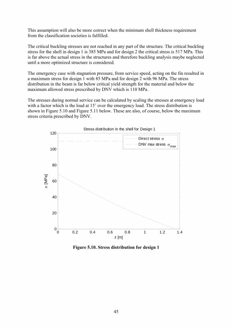
This assumption will also be more correct when the minimum shell thickness requirement from the classification societies is fulfilled. The critical buckling stresses are not reached in any part of the structure. The critical buckling stress for the shell in design 1 is 385 MPa and for design 2 the critical stress is 517 MPa. This is far above the actual stress in the structures and therefore buckling analysis maybe neglected until a more optimized structure is considered. The emergency case with stagnation pressure, from service speed, acting on the fin resulted in a maximum stress for design 1 with 85 MPa and for design 2 with 96 MPa. The stress distribution in the beam is far below critical yield strength for the material and below the maximum allowed stress prescribed by DNV which is 110 MPa. The stresses during normal service can be calculated by scaling the stresses at emergency load with a factor which is the load at 15˚ over the emergency load. The stress distribution is shown in Figure 5.10 and Figure 5.11 below. These are also, of course, below the maximum stress criteria prescribed by DNV.

0 0.2 0.4 0.6 0.8 1 1.2 1.40

20

40

60

80

100

120Stress distribution in the shell for Design 1

σ [M

Pa]

z [m]

Direct stress σDNV max stress σmax

Figure 5.10. Stress distribution for design 1

46

0 0.5 1 1.50

20

40

60

80

100

120Stress distribution in the shell for Design 2

σ [M

Pa]

z [m]

Direct stress σDNV max stress σmax

Figure 5.11. Stress distribution for design 2.

5.4 FEM

5.4.1 Introduction The main purpose of a FE calculation is to evaluate the designs, without structural simplifications, with respect to stresses and eigen frequencies. The eigen frequency analysis are important due to the highly dynamic loading condition that exists behind the propeller. Stresses and loading condition from the FE calculation will also be used in the analysis of the welding and the interface. The model of the fin is created in the modelling tool NX 3.0 see Figure 5.1. The fin model is then exported to the FE software I-DEAS 12 where the pre- and postprocessing is done. The geometry for each design is found from Table 4.2, Table 5.1 and Figure 4.23.

5.4.2 Meshing and boundary conditions Initially the part is partitioned by extruding lines where webs should be. The reason for this is to create a simple model which is easy to mesh with shell elements. The extruded lines create surfaces which directly can be used to mesh on. The element length is of the same magnitude as the plate thicknesses. The foot of the fin is assumed to be clamped all around and therefore all translations and rotations are set to zero along the foot edge. Applied loads are found in Table 4.3. These loads corresponds with the load at ψ=-15˚ which is the highest load acting on the fin and with high number of loading cycles during normal operation and the emergency load. The loads are transformed from forces to uniform pressure acting on the fin. By controlling the reaction forces after simulation it is possible to check if the applied pressure corresponds with the actual loading.

47

The model contains sharp edges and therefore unrealistic discontinuities occur in the FE solution. This is due the singular behaviour at those edges. One way of handling this phenomenon is to use the nominal stress which is used by the classification societies. This is done by simply neglecting unrealistic stresses in the solution and using stresses from the element next to the sharp edge. Another way is to consider stress at a distance from the sharp edge where the singularity is not affecting the stress and extrapolate the stress from a distance to the sharp edge and use that stress in the analysis of the connection between the parts that creates the sharp edge.51

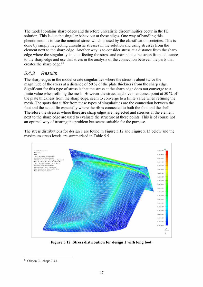
5.4.3 Results The sharp edges in the model create singularities where the stress is about twice the magnitude of the stress at a distance of 50 % of the plate thickness from the sharp edge. Significant for this type of stress is that the stress at the sharp edge does not converge to a finite value when refining the mesh. However the stress, at above mentioned point at 50 % of the plate thickness from the sharp edge, seem to converge to a finite value when refining the mesh. The spots that suffer from these types of singularities are the connection between the foot and the actual fin especially where the rib is connected to both the foot and the shell. Therefore the stresses where there are sharp edges are neglected and stresses at the element next to the sharp edge are used to evaluate the structure at these points. This is of course not an optimal way of treating the problem but seems suitable for the purpose. The stress distributions for design 1 are found in Figure 5.12 and Figure 5.13 below and the maximum stress levels are summarised in Table 5.5.

Figure 5.12. Stress distribution for design 1 with long foot.

51 Olsson C., chap: 9.3.1.

48

Figure 5.13. Stress distribution for design 1 with short foot.

The stress distributions for design 2 are shown in Figure 5.14 and Figure 5.15 and the maximum stress levels are summarised in Table 5.5.

Figure 5.14. Stress distribution for design 2 with long foot.

49

Figure 5.15. Stress distribution for design 2 with short foot.

The FE simulation shows that the stress levels are below the stress levels prescribed by DNV in terms of nominal stresses. Naturally the stress levels are higher in the designs with shorter fin foot.

Table 5.5. Maximum nominal stress levels in the fin.

DESIGN 1 DESIGN 2 Load case Long foot Short foot Long foot Short foot Unit -15˚ 70 75 70 80 MPa 90˚ 90 95 80 90 MPa The stress levels have been calculated for the design scenario which is when the pod has a steering angle of -15˚ and the emergency case. The stresses from the FEA are below the stresses calculated with the simplified beam model but in the same order of magnitude. To evaluate the welding the total stress width is necessary. It will be analysed below but the emergency case will not be included in that analsis. The eigen frequency analysis results are shown in Table 5.6 below. In this analysis the influence from the surrounding water has been neglected and has to be compensated for.

Table 5.6. Eigen frequencies of the different fins.

DESIGN 1 DESIGN 2 Long foot Short foot Long foot Short foot Unit 1st frequency 56 58 51 52 [Hz] 2nd frequency 116 113 122 116 [Hz] 3rd frequency 131 130 181 153 [Hz] 4th frequency 197 187 186 182 [Hz]

50

The eigen frequencies analysis indicates that a shorter fin foot, which is the same as a using weaker boundary condition, gives a higher first eigen frequency. The analysis also indicates that a greater length of the fin gives a lower first eigen frequncy. This is expected according to the ordinary beam theory52. The influence of water has to be considered and the reduction of the eigen frequencies may be done with approximately 25 % which is done for the first eigen frequency in Table 5.7 below.53

Table 5.7. Reduced eigen frequencies of the different fins.

DESIGN 1 DESIGN 2 Long foot Short foot Long foot Short foot Unit 1st frequency 42 43.5 38.25 39 [Hz]

The frequency for a 4 bladed propeller working with a rpm of 150 gives a frequency of 10 Hz which indicates that the third overtone from the propeller may by critical for the design. 5.5 Interface between fin and pod

5.5.1 Introduction The interface between the fin and the cone must be able to carry the loads created by normal service condition but must break before any load in the pod gets high enough to damage the structure. The fin-cone structure is shown in Figure 5.16.

Figure 5.16. Fin and cone principal design, note that the coordinate system shown is the

local system used for FE calculations.

52 Sundström, B, chap: 11.3.5 53 RR staff

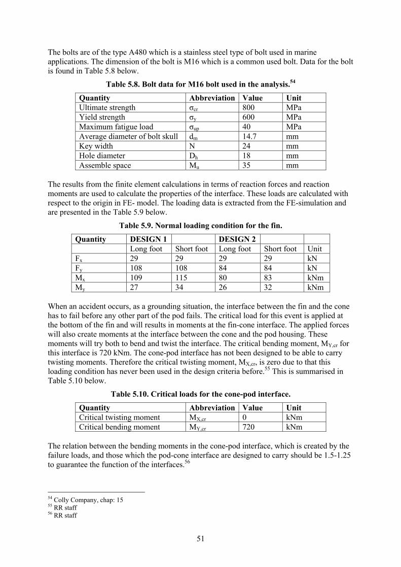
51

The bolts are of the type A480 which is a stainless steel type of bolt used in marine applications. The dimension of the bolt is M16 which is a common used bolt. Data for the bolt is found in Table 5.8 below.

Table 5.8. Bolt data for M16 bolt used in the analysis.54

Quantity Abbreviation Value Unit Ultimate strength σcr 800 MPa Yield strength σy 600 MPa Maximum fatigue load σup 40 MPa Average diameter of bolt skull dm 14.7 mm Key width N 24 mm Hole diameter Dh 18 mm Assemble space Mu 35 mm

The results from the finite element calculations in terms of reaction forces and reaction moments are used to calculate the properties of the interface. These loads are calculated with respect to the origin in FE- model. The loading data is extracted from the FE-simulation and are presented in the Table 5.9 below.

Table 5.9. Normal loading condition for the fin.

Quantity DESIGN 1 DESIGN 2 Long foot Short foot Long foot Short foot Unit Fx 29 29 29 29 kN Fy 108 108 84 84 kN Mx 109 115 80 83 kNm My 27 34 26 32 kNm

When an accident occurs, as a grounding situation, the interface between the fin and the cone has to fail before any other part of the pod fails. The critical load for this event is applied at the bottom of the fin and will results in moments at the fin-cone interface. The applied forces will also create moments at the interface between the cone and the pod housing. These moments will try both to bend and twist the interface. The critical bending moment, MY,cr for this interface is 720 kNm. The cone-pod interface has not been designed to be able to carry twisting moments. Therefore the critical twisting moment, MX,cr, is zero due to that this loading condition has never been used in the design criteria before.55 This is summarised in Table 5.10 below.

Table 5.10. Critical loads for the cone-pod interface.

Quantity Abbreviation Value Unit Critical twisting moment MX,cr 0 kNm Critical bending moment MY,cr 720 kNm

The relation between the bending moments in the cone-pod interface, which is created by the failure loads, and those which the pod-cone interface are designed to carry should be 1.5-1.25 to guarantee the function of the interfaces.56

54 Colly Company, chap: 15 55 RR staff 56 RR staff

52

5.5.2 Model of the interface A principal sketch of the fin-cone interface is shown in Figure 5.17. Geometrical properties are found in Table 4.2 except for r1 which is the smaller radius of the cone and has a value of 250 mm.

L

L 1

r 1

zZZ

z

Figure 5.17. Principal sketch of the fin-cone interface.

The interface is modelled as a plate with a distance to the local origin. The distance is taken as half the distance, L1, from the fin local coordinate system.

53

Figure 5.18. Principal sketch of the fin and the interface.

5.5.3 Method Using basic solid mechanic techniques it is possible to find the point on the fin where the forces are acting. By finding this point it is possible to recalculate the moments that are acting on the interface between fin and cone. These moments are used to evaluate the interface with respect to stresses in the bolts. The differences in bending moments between the case with long and short foot are a result from that the average length between the pressure centre of gravity and the middle of the bolt interface changes, i.e. for the short foot case the lever arm for the forces are shorter than in the case with long foot. The differences in load data are also to be considered. Stresses, from the applied loads, in the interface are calculated according to ordinary beam theory. The stresses from applied loads are then reduced according to (5-21). The stress from the applied load, i.e. the second term of (5-21) is not to be greater than σup as in Table 5.8 to avoid fatigue in the bolt. The critical failure loads for the interface is calculated and then these loads are recalculated to twisting and bending moments for the interface between the cone and the pod housing, see Table 5.10 for allowed loads. This is done until an acceptable design is reached. The influence of the shear force is neglected. The shear force may be carried as friction forces between the interface and the cone. An alternative way of handling this is to install additional shear pins which carry the shear forces but does not make a contribution to the bending stiffness.

5.5.4 Results The results for design 1 with both short and long foot is summarised in Table 5.11-Table 5.12 and Figure 5.19-Figure 5.20.

54

Table 5.11. Results for fin-cone interface for design 1.

Quantity Abbreviation Value Long foot

Value Short foot

Unit

Number of bolts Nb 12 10 - Bending Moment due to lateral load

Mx 71 66 kNm

Bending Moment due to longitudinal load

My 19 21 kNm

The fatigue load criterion is fulfilled in both cases. The failure loads that cause failure of the fin-cone interface are more equal to each other in the case with short foot compared to the case with long foot indicating that a short foot is preferred. Transforming the failure loads of the fin-pod interface to moments at the cone-pod interface indicates that bending moments are above the critical in the interface for the case with long foot, i.e. MY cone > MY,cr but in the case with short foot MY cone < MY,cr naturally MX cone > MX,cr in both cases and has to be taken care of with additional shear elements.

Table 5.12. Results for fin-cone interface for design 1.

Quantity Abbreviation Value Long foot

Value Short foot

Unit

Maximum fatigue load σup 40 38 MPa Failure longitudinal load Fx cr 420 202 kN Failure lateral load Fy cr 175 200 kN Cone twisting load due to Fy cr Mx cone 342 388 kNm Cone bending load due to Fx cr My cone 820 394 kNm

0 0.2 0.4 0.6 0.8 1 1.2 1.4 1.6-0.8

-0.6

-0.4

-0.2

0

0.2

0.4

0.6

0.8

[m]

[m]

Interface fin/cone for c=1.5 with long foot

finbolts

Figure 5.19. Principal sketch of the fin and the interface.

55

0 0.2 0.4 0.6 0.8 1 1.2 1.4 1.6-0.8

-0.6

-0.4

-0.2

0

0.2

0.4

0.6

0.8[m

]

[m]

Interface fin/cone for c=1.5 with short foot

finbolts

Figure 5.20. Principal sketch of the fin and the interface.

The results for design 2 with both short and long foot is summarised in Table 5.13-Table 5.14 and Figure 5.21-Figure 5.22. The differences in loading are discussed above.

Table 5.13. Results for fin-cone interface for design 2.

Quantity Abbreviation Value Long foot

Value Short foot

Unit

Number of bolts Nb 10 10 - Normal Bending Moment due to lateral load

Mx 59 57 kNm

Normal Bending Moment due to longitudinal load

My 21 24 kNm

The fatigue load criterion is fulfilled in both cases. The failure loads that cause failure of the fin-cone interface are equal in the case with short foot compared to the case with long foot indicating that a short foot is preferred. Transforming the failure loads of the fin-pod interface to moments at the cone-pod interface indicates that bending moments are below the critical in the interface for both cases, i.e. MY cone < MY,cr naturally MX cone > MX,cr and has to be taken care of with additional shear elements.

56

Table 5.14. Results for fin-cone interface for design 2.

Quantity Abbreviation Value Long foot

Value Short foot

Unit

Maximum fatigue load σup 40 36 MPa Failure longitudinal load Fx cr 233 122 kN Failure lateral load Fy cr 123 159 kN Cone twisting load due to Fy cr Mx cone 240 310 kNm Cone bending load due to Fx cr My cone 456 237 kNm

0 0.2 0.4 0.6 0.8 1

-0.5

-0.4

-0.3

-0.2

-0.1

0

0.1

0.2

0.3

0.4

0.5

[m]

[m]

Interface fin/cone for c=1.0 with long foot

finbolts

Figure 5.21. Principal sketch of the fin and the interface.

57

0 0.2 0.4 0.6 0.8 1

-0.5

-0.4

-0.3

-0.2

-0.1

0

0.1

0.2

0.3

0.4

0.5[m

]

[m]

Interface fin/cone for c=1.0 with short foot

finbolts

Figure 5.22. Principal sketch of the fin and the interface.

The results indicate that a long foot design will lead to unnecessary high bending moments at the cone-pod interface. If a long foot is preferred for some reason it is necessary to decrease the cord length of the fin or redesign the cone-pod interface to be able to carry much higher moments than today. The critical design aspects for the interface are the failure stresses due to the failure stresses in the rest of the pod structure and the dynamic stresses in the bolt. The difference between the bending stiffness in the x- and y-directions is a problem in the designs with long foot which causes higher failure loads for the fin-cone interface. This means that the rest of the pod structure must be able to carry these loads. The results indicate that a smaller foot is one way of making the interface more suitable for failure in the longitudinal direction, as in Figure 5.18. This is naturally due to the decrease of the Steiner contribution which scales with the square of the distance between the element and the centre of gravity. In the case with short foot, the part of the fin which is behind the foot may deflect against the cone and create a support which will increase the lever arms for the bolts. This will result in much lower stresses in the bolts hence will the moment on the cone-pod interface be very high before the critical stress in the bolts is reached. One way of treating this problem is to ensure that the distance between the fin and the cone at the part behind the fin foot is great enough to ensure that a support is not created when a longitudinal load is applied. The distance may be filled with a soft deformable material which allow the fin to maintain its hydrodynamic function at the same time as it does not creates a support for the part of the fin behind the interface.

58

5.6 Fatigue in welding Since the structure is manufactured with welding as joining technique and the loading condition is highly dynamic with high number of load cycles, fatigue is likely to occur in the weld. A fatigue analysis of the weld therefore has to be performed. Due to the much higher area moment of inertia in the longitudinal direction of the fin cross section a reasonable assumption is that the stress level in the fin scales linear with the applied lateral force. By this assumption it is possible to calculate the stress level at any lateral load if the stress at one loading condition is known. The stress width is calculated as the absolute difference between the stresses created by lateral forces acting on the fin.57 The loading of design 1 is shown in Table 4.4 and corresponding stress widths are shown in Table 5.15.

Table 5.15. Stress widths of design 1 with short foot.

Steering angle Unit Quantity Abbreviation ±35˚ ±15˚ ±5˚ ±2˚ deg Stress width, short foot σr,s 125 95 42 17 MPa Number of cycles58 N 1500 106 2·106 2·107 -

A load spectrum for design 1 with short foot as in the tables above is shown in Figure 5.23 below. Even if the load spectrum is asymmetric it is the total stress width that is considered in the analysis. The load spectrum in Table 5.15 shows that there are high stress levels at a high number of cycles, i.e. at steering angles of ±15˚. This corresponds to about 100 cycles a day during a life time. This number might be a little bit too high and should be investigated further. As an example, handbooks indicate that a hull bottom has a spectrum parameter of 0 and a life time of order 108 loading cycles.59 This indicates that the load spectrum for a hull bottom contains all varieties of loads and that they are linear proportionally to each other and that the structure is loaded with very small forces at a high number of cycles.

57 SSAB, chap: 5.2. 58 RR staff 59 SSAB, chap: 5.2.

59

2 3 4 5 6 7 80

0.2

0.4

0.6

0.8

1

1.2

σr/ σ

r,max

log N

Loadspectrum for fin

Loads short footLinear load spectrum p=5/6Linear load spectrum p=2/3Linear load spectrum p=1/2Linear load spectrum p=1/3Linear load spectrum p=1/6

Figure 5.23. Actual load spectrum with a linearization of the same.

Independently of which design or type of foot that is considered, the load spectrum will have the same shape in all cases. The reason for this is that all forces scales linear with the cord length and the assumption that the stress level scales linear with applied lateral load. This means that it will always be the ±15˚ loading condition that determines the load spectrum parameter. It is possible from the Figure 5.23 above to extract the load spectrum parameter. The parameter is extracted from the line that best approximates the load spectra. Choosing the line which corresponds to p=2/3 and using Figure 5.4 for that value of p gives an allowed stress range between 65-75 MPa depending on which probability of failure that is considered. Using a high probability of fracture and a high quality weld will not lead to an acceptable stress width. High probability seems reasonable since the ship will be controllable even if the fin is lost from the pod. But a high quality weld is probably not possible to achieve. The weld quality and therefore the load directional factor, KX, may be discussed further. The load directional factor has to be increased if several weldings interacts as in the case where the fin-shell, foot- and web are joined together. Therefore the solution with a welded joint between the fin and its foot seems unrealistic if not the local design of the joint is changed in a more sufficient way. One way of handling the problem is to use a smooth transition between the foot and the fin. However, this requires a solution with smooth transition double curvature plates which will increase the manufacturing costs due to the need of expensive tools for creating the shape. Only design 1 with the short foot is evaluated in terms of fatigue. The reason for this is that design 1 with short foot seems to have greatest potential to fulfil the requirements of a fin that

60

should be fitted to a pod. But the results will be useful for the other designs hence the load spectrum will have the same shape for all designs. 5.7 Conceptual structural design The loading condition is highly dynamic which implies that fatigue is likely to occur in the welding and in the bolts. Sharp edges should be avoided as far as possible due to their ability to create areas where high stresses occur. Critical design parameter of the fin structure is the stress width of the welding and of the bolts. One option is of course to use thicker plating but probably there is need for a smooth transition between the fin and foot which will require special tools during manufacturing. The interface between the fin and the pod should not be of the same length as the cord of the fin, i.e. the interface should have a low aspect ratio, length over width. This will make the bending stiffness more equal in all direction. Due to the geometric shape of the fin the distances from bolt to centre of gravity along the fin will be greater than the lateral distances if the interface is not shortened. The problem with a possible support of the fin against the cone has to be evaluated further. The recommended design is a fin according to design 1 with short foot. Short interface makes the critical failure loads more equal and there is no need for additional bolts in the cone-pod interface but additional shear pins have to be added to carry the twisting moment. A conceptual sketch of the fin is found in Figure 5.24 below. Scantlings of the fin are found in Table 4.2 and Table 5.1. Properties of the construction material are found in Table 5.2. The fin-cone interface details are found in Table 5.8, Table 5.16 and Figure 5.19.

Table 5.16. Fin foot properties.

Quantity Abbreviation Value Unit Height of foot Hf 550 mm Length of foot Lf 750 mm

The most critical aspect within the design is the welding between the fin and the fin foot which has to be redesigned and investigated further.

61

c

L

L 1

Lf

Hf

tw

ts

2tf

0.25c

Figure 5.24. Fin conceptual design.

5.8 Future work The actual loading condition for the fin has to be analysed and refined. This means that a more detailed hydrodynamic analysis has to be performed. A more detailed load spectrum is probably necessary for analysis of the fatigue aspects in the structure. This also includes alternatives in the design to handle the problem of stress concentrations in the areas of welding. For example designing the structure in a more smooth style that minimizes the area where stress concentrations may occur. The redesigning of the cone at the area where the fin should be attached has not been considered. This includes local stiffening system to transport fin loads into the structure and the influence on the cone if a short fin-foot interface is used. The latter has to be evaluated in terms of corrosion in the small distance between the fin and the cone. Another aspect is how the classification societies handle the fin construction whether the rudder rules are applicable on the construction which has been the assumption in this thesis work.

62

6 Economy Contacts with the manufacturer "Degerfors Formnings AB" resulted in a price proposal which is based on the design 1 see Figure 4.23 for a general view. The welding length of that design is approximate 12m and the total weight of the design is about 800 kg. The cost approximation contains all kinds of work e.g. material, painting, preparations before welding, welding, quality check of welding and processing the fin foot for connection the fin with the cone. A rough approximation of the total costs is 100 kkr.60 This estimation is based on an assumption that the shell is split into four pieces and then joined with the rib and the fin foot. Assuming that approximately 34 % of the price is material costs, including overhead and earnings, and that 66 % of the price is manufacturing costs it is possible to roughly estimate the manufacturing costs per length of weld.61 This assumes that the working costs scales with the welding length and the material costs scales with the weight of the fin. This is not completely true but seems to be a reasonable approximation when all work except the forming process, e.g. cutting, welding and quality check, depends on the welding length and the material costs scales directly with the amount of material.62 This means that the production costs may be divided into two parts one that depends on the material weight and one that depends of the welding length. Using the data described above gives a material cost of about 43 SEK/kg material and a work cost of 5500 SEK/m weld. This reasoning gives that it is more cost efficient to use more material compared to trying to reduce the weight using a complex stiffening system which creates a lot of welding meter. In other words each extra meter welding has to be compensated with a weight reduction of at least 130 kg material which seems highly unrealistic even to be considered. The conclusion that could be drawn from this is that a structure with a minimum of welding would be preferred. However there are costs with a fin that is not covered in the manufacturing costs e.g. additional costs in terms of redesigning the cone with a local stiffening system where the bolts from the fin-cone interface should be fastened; or redesigning the cone-pod interface to be able to carry the new loads produced from the fin installation and additional maintenance costs. These costs are not covered in this analysis and have to be investigated further. Other construction possibilities as slot welding and a shell which is split into just two pieces may be an alternative but is not covered here. The benefit from a fin installation is that the need for azimuth moment during operation will decrease. This will allow a redesign of the steering gear equipment and therefore a less expensive installation can be used. Approximate calculations indicates that a reduction of the azimuth moment with 25 % will give a reduction of the costs from the steering gear equipment with 100 kkr and a 50 % reduction will gain a cost reduction of 200 kkr.63 Calculations are made for a installation with 2 pods.

60 Ström J., Deform AB 61 RR staff 62 RR staff 63 RR staff

63

Economic benefit from a higher propulsive efficiency of 0.5 %, indicated in the hydrodynamic calculations, in terms of fuel savings is neglected in the study above. However a rough estimation of the gain from fuel savings during a life time can be done for the 10 MW pod which is assumed to have a lifetime of 25 years and a usage of 6000 h/year. Assuming that the power needed in normal service speed is 85 % of the available power gives a saving in power of approximate 40 kW. During a lifetime this corresponds with an energy saving about 6 GWh or 22·106 MJ. Energy available in marine diesel is approximate 40 MJ/kg64 and with a assumed combustion efficiency of 50 % gives a total saving in diesel fuel of approximate 1100 Metric Tonne, MT. The cost for 1 MT marine diesel is approximate 800 $65 which gives a total saving in fuel costs of 880 000 $ per pod during a lifetime. Effects on the propeller efficiency has not been considered in this analysis. The conclusion from this is that the azimuth moment has to be reduced by at least 50 % if the costs from a fin installation should be balance by a cost reduction in the steering gear equipment. If the whole life time of the ship is considered, a fin attached to the pod seems to be highly motivated in terms of fuel savings, not to mention the benefits from trying to reduce the consequences for the environment in terms of goodwill for the shipping company in question. Alternative solutions of the fin construction material have to be analysed and evaluated. Are there any way of cutting down the production costs by using more exotic materials as composites?

64 Andersson, T., chap: 3.3 65 www.bunkerworld.com, 2008-01-22

64

7 Summary and discussion In this master thesis work a fin has been considered in terms of hydrodynamics, structure and economics. This has resulted in a proposal of a conceptual fin design. This proposal should be considered as a first recommendation that can be refined further. A fin according to design 1 with short foot seems to be the best solution to reduce the hydrodynamic momentum. The fin should be mounted as far back on the pod as possible at a six a clock position. The size of the fin is dependant of the size of the pod and the propulsive power. On a 10 MW pod the cord of the fin will be 1.5 meters and the span at the leading edge 1.1 meter and at the trailing edge 1.5 meters. 7.1 Hydrodynamic Hydrodynamically the biggest issue, which in principal is not considered at all, is cavitation. This phenomenon could create problems like corrosion on the fin and should be considered in a more refined design. In the hydrodynamic model used, only a flow around a wing attached to a wall is considered, where velocities representing the propellers swirl are added to the free stream velocity. The added swirl is an estimate that approximates the result of a cavitation tunnel test made by Rolls Royce.66 Calculations have been done at constant speed. If the ship is accelerating or decelerating the propeller slipstream and swirl will be different. Because of this, studies have to be made in these conditions too. Preferably CFD or cavitation tunnel test. When fitting a pod with a fin the whole flow field of the pod is changed. This has consequences for the propeller too. So, if a propulsion system with optimum performance should be developed the propeller and fin interaction has to be considered also in the design of the propeller. Other ways to try to make the fin more efficient is to make the fin cambered or having different profiles along the length of the fin. Such changes could maybe give a better lift to drag ratio for the fin. There could possibly be some gain in letting the fin extend outside the given limits i.e. not deeper than the propeller and not further back than the pod housing. A fin that is swept backwards could then be larger, generate more lift, and have a longer lever arm hence increasing the two variables that determine the momentum. 7.2 Structure Mechanically one of the greatest issues is the stress concentration in the weld between the foot and the fin, here a better shape could probably solve the problem and has to be investigated further. This problem may be solved if different concepts in material are considered. For example in a sandwich structure the foam may be formed in a very simple way therefore the fin can easily be formed as wanted.

66 Johansson, R., New Generation Pod

65

Combinations of materials may also be a solution for the fin. Using a fin in sandwich and a fin foot in casted steel which are glued together may be a solution to consider. The fin foot may be constructed to fit different pod sizes and the fin can be design for the actual purpose in a more efficient way. One other problem in the optimisation process is the regulations from the classification societies. The regulations state the minimum plate thickness for a given structure and therefore the material may not be used in the most efficient way. The minimum plate thickness regulation is not negotiable which means that, even if the stress levels in the structure are far below the acceptable, it must be shown in a high detailed level that the regulations are not suitable for the case. 7.3 Economy The fin is considered as a stiffened thin wall construction with a symmetric wing profile. The benefit of using these sorts of structures is that the material usage may be efficient but in addition to this a complex structure may also be difficult to manufacture. This means that the optimisation with respect to weight reduction must not be pushed too far. The fin should be constructed with a minimum of parts which needs to be welded. It is in general cost efficient to use more material and less complicated stiffening system, even though the weight will increase. One benefit of low weight is that it would be easy to handle the fin during dockings in maintenance situations but some sort of lift will probably have to be used anyhow. One thing to refine is the economical estimation. First of all a better price estimation of material cost versus welding cost has to be created to enable optimisation of the cost of the fin. A more detailed cost analyse of the whole system has to be performed. It should at least cover:

• Manufacturing costs for the fin • Costs for redesigning the cone to be able to carry the fin and the interface between the

cone and the pod • Cost reduction due to smaller steering gear equipment • Consequences for the fuel consumption • Consequences for maintenance cost.

One design alternative is to maximise the increase in propulsive efficiency and compare the reduction in operational costs with the additional costs from a fin installation during a life time of the pod.

66

8 References 8.1 Published material

Abbott, I., "Theory of wing sections", 2nd edition, Dover publications ltd., New York, 1959. Andersson, S., "Systemutveckling – Funktionsprinciper, mekaniska komponenter och gränssnitt", KTH, Department for machine design, Stockholm, 2004. (In Swedish) Andersson, T., " Maskinlära för sjöpersonal", TA-driftteknik, Stockholm, 1992. (In Swedish) Bergkvist. L., "Konstruera med EHS- och AR-plåt", Svenskt Stål division grovplåt, Oxelösund, 1997. (In Swedish) Bonde-Wiiburg, E., "Karlebo Handbok" 15th edition, Liber, 2000. (In Swedish) Çelik, F., Güner, M., "Energy saving device of stator for marine propellers", Yildiz Technical University, Department of naval architecture, Istanbul, 2006. Colly Company AB, "Handbok om skruvförband", Colly Company division maskinelement, Stockholm, 1995. (In Swedish) Det Norske Veritas, "Rules for classifications of ships", Det Norske Veritas, Høvik, 2007. Huss, M., "Förläsningsanteckningar i skrovkonstruktion", KTH Centre for Naval Architecture, Stockholm, 1999. (In Swedish) Ishida, S., "The Recovery of Rotational Energy in Propeller Slipstream by Fins installed after Propellers", JSNA Japan Vol.159, 1986. Li, D-Q., Dyne, G., "Study of Propeller-Rudder Interaction based on a Linear Method", Ship building in progress, vol 42 n 431, Sept 1995 p 235. Marchaj C. A., "Aero- Hydrodynamics of Sailing", 3rd edition, Miller Publishing, Part 2, Lloyd's Register, "Rules and regulations for the classification of ships", Lloyd's Register, London, 2004. Megson, T.H.G., "Aircraft structures for engineering students", 3rd edition, Elsevier Butterworth Heinemann, Oxford, 1999. Olsson, C., "Dimensionering av svetsade konstruktioner", Sveriges verkstadsindustrier, Uppsala, 1993. (In Swedish) Rawson, K.J., Tupper, E.C., " Basic Ship Theory", 5th edition, Butterworth Heinemann, Oxford, 2001. Råde, L., Westergren B., "Mathematics handbook for science and engineering", 4th edition, Studentlitteratur , Lund, 1998.

67

Sundström, B., "Handbok och formelsamling i hållfasthetslära", KTH, Department for solid mechanics, Stockholm, 1998. (in Swedish). Young, W.C., Budynas, R.G., "Roark's formulas for stress and strain" 7th edition, McGraw-Hill, 2002. Zenkert, D., "Plate theory",2nd edition, KTH Division of lightweight structures, Stockholm, 2006.

8.2 Non-published material Bohm, M., "Reducing of the steering moment of the AZIPULL pulling thruster system from Ulstein Propeller AS with a fin", report no. 2456, 1999 http://www.vacantisw.com/foildesign.htm Johansson, R., "New Generation Pod T-32", report PR-1163, 2006 Rolls-Royce, Personal within the pod division. Ström, J., "Degerfors Formings AB" Xfoil, Mark Drela, MIT Aero & Astro, Harold Youngren, Aerocraft, Inc. , http://web.mit.edu/drela/Public/web/xfoil/