FEniCS CourseLecture 20: Tools for visualizationprogramming

ContributorsCarl Lundholm, Magne Nordaas

1 / 22

Visualisation in FEniCS

Three main options for visualisation

• Built-in VTK plotting

• matplotlib

• ParaView

2 / 22

Built-in VTK plottingBuilt-in plotting functionality for FEniCS

• Plot meshes, functions, mesh functions• Not available on all FEniCS installations• Limited 3D capabilities

from fenics import *

parameters["plotting_backend"] = "vtk"

mesh = UnitCubeMesh(16, 16, 16)

plot(mesh)

interactive ()

3 / 22

matplotlib

Plotting libarary for Python and Numpy

• Part of a standard Python installation

• Has a MATLAB-like interface

• Produces high-quality 1D and 2D plots

Related projects

• Pandas

• Seaborn

4 / 22

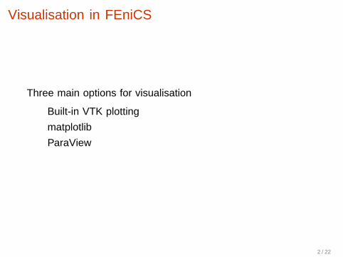
matplotlib example

from dolfin import *

from matplotlib import pyplot

parameters["plotting_backend"] = "matplotlib"

mesh2D = UnitSquareMesh(16,16)

mesh3D = UnitCubeMesh(16, 16, 16)

plot(mesh2D)

plot(mesh3D)

pyplot.show()

5 / 22

6 / 22

matplotlib example II

# appended to Cahn -Hilliard demo

parameters["plotting_backend"] = "matplotlib"

from matplotlib import pyplot

# call the plot command from dolfin

p = plot(u[0])

# set colormap

p.set_cmap("viridis")

p.set_clim(0.0, 1.0)

# add a title to the plot

pyplot.title("Cahn -Hilliard solution")

# add a colorbar

pyplot.colorbar(p);

# save image to disk

pyplot.savefig("demo_cahn -hilliard.png")

7 / 22

matplotlib example II

8 / 22

matplotlib with FEniCS on mac and Windows

Displaying figures are more difficult when using a Dockerinstallation of FEniCSThe options are:

1 Saving figures to file and open them on the host system(inconvenient)

2 Use Jupyter Notebook:Create and start a Docker container with the commands

Bash code

fenicsproject notebook fenics -nb stable

fenicsproject start fenics -nb

Direct your web browser to address and port numberprinted to the screen

9 / 22

Jupyter Notebook

Jupyter Notebook is part of the Project Jupyter(www.jupyter.org), which evolved from IPython.

• Web application

• Provides interactive environment for Python code (andother languages!)

• Combine code, equations and visualisation in oneinteractive document

To display figures inside the notebook, add this line to thenotebook:

%matplotlib inline

10 / 22

ParaView

ParaView is a freely available, open source, multi-platform datavisualisation application.

• Publication-quality figures

• Provides sophisticated data analysis functions• Stream lines• Time averages• Isosurfaces• ... and much more

• Can handle very large (and parallelized) data sets

• Support data file formats used by FEniCS:• ParaView files (.pvd)• VTK files (.vtu)• XDMF files (.xdmf)

11 / 22

ParaView resources

Official site: www.paraview.org

• Binaries for mac, ubuntu,windows

• ParaView tutorials

• The ParaView Guide

12 / 22

Using ParaView with FEniCSConsider following example solving a Poisson problem:

from dolfin import *

mesh = UnitCubeMesh(16, 16, 16)

V = FunctionSpace(mesh , "P", 1)

u = TrialFunction(V)

v = TestFunction(V)

f = Constant(1.0)

a = inner(grad(u), grad(v)) * dx

L = f * v * dx

bc = DirichletBC(V, 0.0, "on_boundary")

uh = Function(V)

solve(a == L, uh , bc)

How can we visualise the solution?13 / 22

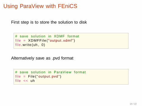
Using ParaView with FEniCS

First step is to store the solution to disk

# save solution in XDMF format

file = XDMFFile("output.xdmf")

file.write(uh, 0)

Alternatively save as .pvd format

# save solution in ParaView format

file = File("output.pvd")

file << uh

14 / 22

Using ParaView with FEniCS

Start ParaView and open the file (Button in top left corner)

After opening the file click the Apply button

15 / 22

Using ParaView with FEniCSYour screen should look similar to this:

After opening the file click the Apply button16 / 22

Using ParaView with FEniCS

ParaView has a nice GUI so you can easily play around withthe many functions and settings available.

The functions for slicing, and contours and streamlines areparticularly useful for 3D data:

Save results using File->SaveScreenshot orFile->ExportScene from the menu.

17 / 22

Good practices for visualisation of data

Automate visualisation (and other post-processing) with Pythonscripting.

• Ensures consistent results

• Saves time

• With ParaView: Manually make your figures once usingthe GUI. You can save the state (File->SaveState) andreuse it your python scripts.

Separate post-processing from solver code.

18 / 22

Saving data to files

Save data for plotting in XDMF or paraview formats:

uh = Function(V)

# saving uh to XDMF file

xdmf_file = XDMFFile("output.xdmf")

xdmf_file.write(uh , 0)

# saving uh to ParaView file

pvd_file = File("output.pvd")

pvd_file << uh

19 / 22

Saving data to filesDifferent formats have to be used for reading from file:

# saving to HDF5 file

hdf5_file = HDF5File(mpi_comm_world (), \

"output.hdf5", "w")

hdf5_file.write(uh , "solution")

# saving to compressed XML file

xml_file = File("output.xml.gz")

xml_file << uh

We can read from these files at later time:

# reading from HDF5 file

hdf5_file = HDF5File(mpi_comm_world (), \

"output.hdf5", "r")

hdf5_file.read(vh , "solution")

# reading from compressed XML file

xml_file = File("output.xml.gz")

xml_file >> vh

20 / 22

Writing/reading meshes and meshfunctionsA FEniCS Mesh or MeshFunction are handled similarly:

mesh = UnitSquareMesh(16, 16)

mf = MeshFunction("size_t", mesh , 0)

# Save mesh data:

hdf5_file = HDF5File(mpi_comm_world (), \

"mesh_data.hdf5", "w")

hdf5_file.write(mesh , "Mesh")

mvc = MeshValueCollection("size_t", mesh , mf)

hdf5_file.write(facet_domains , "Mesh/SubDomains")

Reading saved mesh data:

hdf5_file = HDF5File(mpi_comm_world (), \

"mesh_data.hdf5", "r")

# read mesh data

mesh = Mesh()

hdf5_file.read(mesh , "Mesh", False)

mvc = MeshValueCollection("size_t", mesh , 0)

hdf5_file.read(mvc , "Mesh/SubDomains")

mf = MeshFunction("size_t", mesh , mvc)

21 / 22

Exercises

1 Modify the nonlinear Poisson solver to solve a problem ona UnitCubeMesh

2 Try to make some nice figures of the 3D data usngParaView. Experiment with slices and contours, and trychanging the colormap.

3 Visualise the output of the hyperelasticity solver.Experiment with (glyphs arrows to represent vectors) andthe warp-by-vector function.

22 / 22