
Feedback and control of micro-pumps - Swinburne · Feedback and Control of Micro-pumps Submitted by...
283
Feedback and Control of Micro-pumps Submitted by Tom Tomac This Thesis is submitted in fulfilment of the requirements of the degree of Doctor of Philosophy in the school of Advanced Studies at Industrial Research Institute Swinburne (IRIS) Swinburne University of Technology March 2002
Transcript of Feedback and control of micro-pumps - Swinburne · Feedback and Control of Micro-pumps Submitted by...

Feedback and Control of Micro-pumps
Submitted by
Tom Tomac
This Thesis is submitted in fulfilment of the requirements
of the degree of Doctor of Philosophy
in the school of Advanced Studies
at
Industrial Research Institute Swinburne
(IRIS)
Swinburne University of Technology
March 2002

i
ACKNOWLEDGMENTS
The author would like to thank Dr. Dario Toncich, Deputy Director of Advanced
Studies at The Industrial Research Institute Swinburne (IRIS), Swinburne University of
Technology for guidance and support over the period of this research. His commitment
to the supervision has been exemplary, for which, I extend my deepest gratitude.
In addition, the author thanks Dr. Paul Stoddart and Dr. Alex Mazzolini of
Centre for Imaging and Applied Optics (CIAO) at School of Biophysical Sciences and
Electrical Engineering (BSEE) Swinburne University of Technology, for the technical
support in the field of optics.

ii
DEDICATIONS
This thesis is dedicated to a number of close family members like my mum
Josipa and my dad Zlatko, who have gone the distance and are always in my thoughts,
my sisters Lily and Mary who unselfishly and unconditionally helped mum and dad
during their time of need, my son Daniel with energy and enthusiasm that will
undoubtedly help him open many doors in his life, and my darling wife Pam, who
supported me throughout all the frustrations, tantrums, sleepless nights and absenteeism
from all those special occasions that I unknowingly took for granted.
I dedicate this thesis to the preservation of family values and faith in the whole
of humanity in the quest for the betterment of oneself.

iii
Table of Contents
1 Introduction ................................ ................................ ................................ .......... 1
1.1 Overview ................................ ................................ ................................ ...... 2
1.2 Background................................ ................................ ................................ ... 5
1.3 Central Research Theme ................................ ................................ ............... 9
1.4 Overview of Methodology ................................ ................................ .......... 12
1.5 Overview of Experimental Procedures ................................ ........................ 13
1.5.1 Development of Laboratory-on-a-Board................................ .......... 13
1.5.2 Micro-pump Characterisation................................ .......................... 14
1.5.3 Closed-loop Control................................ ................................ ........ 16
1.5.4 Integration Considerations ................................ .............................. 17
1.6 Perceived Contributions ................................ ................................ .............. 19
1.7 Thesis Structure ................................ ................................ .......................... 21
2 Literature Review ................................ ................................ ............................... 22
2.1 Overview of Review Process................................ ................................ ....... 23
2.2 A Historical Perspective on Micro-Pump Systems................................ ....... 25
2.3 Design, Modelling and Testing of Micro-Pumps ................................ ......... 28
2.4 Actuation of Micro-Pumps, including the Magnetic Membrane................... 39
2.5 Piezoelectric Devices and Characterization ................................ ................. 44
2.5.1 Optimisation Of A Circular Piezoelectric Diaphragm For A Micro-
pump 44
2.5.2 Piezoelectric Ceramics as In-Plane Actuators................................ .. 47
2.5.3 Piezoelectric Actuator Having Stable Resonant Frequency.............. 52
2.6 Optical Coherence Tomography (OCT)................................ ....................... 54
2.7 Photodiodes ................................ ................................ ................................ 56
2.8 Fibre-Optics ................................ ................................ ................................ 58
2.9 Open-loop Characterisation of Micro-pumps................................ ............... 62
2.10 Integrated Optical Directional Couplers in Silicon-on-Insulator................... 70
2.11 Integrated Optical Sensor Considerations ................................ .................... 77
2.12 Summary of Literature Review................................ ................................ .... 80
3 Design and Construction of Open and Closed-loop Test Platforms...................... 83
3.1 Overview ................................ ................................ ................................ .... 84
iv
3.1.1 Design Sequence and Rationale ................................ ...................... 84
3.1.2 Characterisation of a Piezoelectric Actuator Using a Low-Coherence
Interferometer ................................ ................................ ................................ ..... 86
3.2 The Micro-pump ................................ ................................ ......................... 90
3.2.1 General ................................ ................................ ........................... 90
3.2.2 Micro-pump Operation ................................ ................................ ... 91
3.3 The Fibre Optic Interferometer Construction................................ ............... 93
3.4 Development of Electronic Test Platform................................ .................... 98
3.4.1 Overview ................................ ................................ ........................ 98
3.4.2 Detection Elements and Parameters ................................ ................ 98
3.4.3 Photodetectors ................................ ................................ ................ 99
3.4.4 Photodiode Amplifiers ................................ ................................ .. 100
3.4.5 Instrumentation Amplifier................................ ............................. 103
3.4.6 Data Acquisition ................................ ................................ ........... 105
3.4.7 Analog Input Range ................................ ................................ ...... 108
3.4.8 Driving the Analog Inputs................................ ............................. 110
3.4.9 Data Interfacing ................................ ................................ ............ 111
3.4.10 Ground and Layout ................................ ................................ ....... 112
3.4.11 Data Processing Hardware ................................ ............................ 113
3.4.12 FPGA - ADC Interface ................................ ................................ . 117
3.4.13 FPGA – FIR Filter ................................ ................................ ........ 118
3.4.14 FPGA Memory Requirement ................................ ........................ 120
3.4.15 FPGA Serial Communications Interface................................ ........ 123
3.4.16 Piezoelectric Driver ................................ ................................ ...... 126
3.4.17 Integrated Open and Closed-loop Test Platform ............................ 130
4 Open and Closed-loop Experimental Methodology ................................ ........... 133
4.1 Frequency Extraction Method ................................ ................................ ... 134
4.2 Actuator Direction Extraction Method................................ ....................... 135
4.3 Actuator Pulse Shaping Technique ................................ ............................ 136
4.4 Signal and Data Processing Technique ................................ ...................... 139
4.5 Photonic Conversion Extraction ................................ ................................ 140
4.6 Displacement and Trigger Detection Method ................................ ............ 144

v
4.6.1 Direction Decoder Considerations................................ ................. 145
4.6.2 Frequency Counting Method................................ ......................... 145
4.7 Closed-loop Control Methodology ................................ ............................ 149
4.8 Micro-pump Closed-loop Experimental Considerations............................. 150
4.9 Closed-loop Controlling Elements and Parameters ................................ .... 151
4.10 Control Logic and Transfer Function Considerations................................ . 153
4.11 Analysis and Control Electronics................................ ............................... 166
4.12 Displacement Verification Method................................ ............................ 168
5 Open and Closed-Loop Experimental Results ................................ ................... 171
5.1 Open-Loop Overview................................ ................................ ................ 172
5.2 Open-loop Experimental Outcomes................................ ........................... 173
5.3 Open-loop Result Summation................................ ................................ .... 183
5.4 Closed-loop Experimental Outcomes ................................ ........................ 185
5.5 PZT Driver Closed-loop Feedback Analysis................................ .............. 197
6 Open and Closed-loop Comparison Analysis................................ ..................... 207
6.1 Open-loop / Closed-loop Comparison Analysis ................................ ......... 208
6.2 Comparison Summary................................ ................................ ............... 213
6.3 Integration Issues ................................ ................................ ...................... 214
7 Conclusions and Recommendations ................................ ................................ .. 218
7.1 Overview ................................ ................................ ................................ .. 219
7.1 Specific Contributions................................ ................................ ............... 220
7.2 Enveloping Broad-Context Discussion ................................ ...................... 222
7.2.1 Characterisation and Open-Loop Performance .............................. 222
7.2.2 Closed-Loop Performance................................ ............................. 224
7.2.3 Summary Comparison Between Open-Loop and Closed-Loop Control
226
7.2.4 Overall Summary................................ ................................ .......... 229
7.3 Limitations of Research................................ ................................ ............. 230
7.4 Recommendations for Further Research ................................ .................... 231
NOMENCLATURE…………………………………………………………………..221
REFERENCES………………………………………………………………………..222

vi
Table of Appendices
Appendix – A Conference Proceedings……………………………………... A-1
A.1 SPIE Conference………………...…………………………………....A-1
Appendix – B Technical Information and Data associated with the Embodiment
of this Research…………………………………………….....B-1
B.1 Circuit Diagrams……………………………………………………....B-1
B.1.1 FPGA Device………………………………………………….B-1
B.1.2 CPU + Memory……………………………………………….B-1
B.1.3 Optical ADC Interface………………………………….……..B-2
B.1.4 Serial ADC Interface………………………………………….B-2
B.1.5 Optical Amplifier Interface…………………………………...B-2
B.1.6 Serial DAC Interface………………………………………….B-3
B.1.7 High Voltage Generator…………………………………….…B-3
B.1.8 PZT Shaper Interface……………………………………….…B-3
B.1.9 Peripheral Interface Unit (PIU)……………………………….B-4
B.1.10 Power Distribution Module (PDM)…………………………...B-4
B.2 Test Results Data……………………………………………………...B-4
B.2.1 Open-loop Air Data…………………………………………...B-5
B.2.2 Open-loop Water Data……………………………………..….B-5
B.2.3 Open-loop Water+28% Glycerol Data……………………..…B-6
B.2.4 Open-loop Water+60% Glycerol Data……………………..…B-6
B.2.5 Closed-loop Air Data……………………………………….....B-7
B.2.6 Closed-loop Water Data…………………………………..…..B-7
B.2.7 Closed-loop Water+28% Glycerol Data………………..…..…B-8
B.2.8 Closed-loop Water+60% Glycerol Data……………..……..…B-8
B.2.9 Closed-loop Air PZT Driver variation displacement
and modulation data…………………………………………...B-9
B.2.10 Closed-loop Water PZT Driver variation displacement
and modulation data………………………………………..….B-9
B.2.11 Closed-loop Water+28% Glycerol PZT Driver variation
displacement and modulation data………………………….....B-9

vii
B.2.12 Closed-loop Water+60% Glycerol PZT Driver variation
displacement and modulation data…………..………..……...B-10
B.2.13 Open-loop Combination Result Data………...……….….….B-10
B.2.14 Closed-loop Combination Result Data……………………....B-10
B.2.15 Closed-loop PZT Driver Area Result Data………….………B-10
B.2.16 Open and Closed-loop Combination Result Data…………...B-11
B.3 System Components Data Sheets……………………………………B-11
B.3.1 Optical Interface……………………………………………..B-11
B.3.2 Amplifier Interface…………………………………………..B-11
B.3.3 ADC……………...…………………………………………..B-12
B.3.4 DAC……………...…………………………………………..B-12
B.3.5 FPGA………………………………………………………...B-12
B.3.6 Micro-controller….…………………………………………..B-13
B.3.7 Memory………….…………………………………………..B-13
B.3.8 Communications Interface……………………………….….B-13
B.3.9 Application Specific Standard Products (ASSP)...……….….B-13
B.3.10 Power…………….…………………………………….…….B-14
B.4 Firmware Algorithms…………...……………………………….…..B-14
B.4.1 FIR Filter Function……………………………………….….B-14
B.4.2 Photonic Conversion Function..………………………….….B-14
B.4.3 Trigger Function…………………………………………….B-15
B.4.4 Direction Finder Function..…………………………….…....B-15
B.4.5 Frequency Counting Function………………...………….….B-16
B.4.6 Error Variation Function…………...…………………….….B-16
B.4.7 Sub Function Modules………………………..…………..….B-16
B.5 Software Algorithms…………...………………………….……..…..B-18
B.5.1 Displacement Algorithm Function…………………….…….B-18

viii
Table of Tables
Table 2.1 - Comparisons of the Performance of the Three Transducer Configurations
(abstracted from Harrison et al., 1999) ................................ ................................ 50
Table 3.1 - Photodiode Characteristics................................ ................................ ........ 99
Table 5.1 - Flow Rate / Displacement vs. Frequency data table................................ . 181
Table 5.2 - Open-loop Response for Frequencies Ranging from 10 Hz to 100 Hz and
Four pumping media (air, water, water+28% and 60% glycerol) ....................... 183
Table 5.3 - 10Hz PZT Driver Amplitude Variation Effect for Water ......................... 201
Table 5.4 - Closed-loop Response for Frequencies Ranging from 10 Hz to 100 Hz and
Four Pumping Media (air, water, water+28% and 60% glycerol)....................... 204
Table 6.1 - Average Difference Between Open and Closed-loop Data for the
Displacement of Differing Media ................................ ................................ ...... 209
Table 6.2 - Flow Rate Comparison Between Open and Closed-loop System Based on
the data of Tables 5.2 and 5.4................................ ................................ ............ 211
Table 6.3 - Open and Closed-loop Average Percentage Variation Comparison Table 212
Table 6.4 - Integrated System Block Descriptions................................ ..................... 217

ix
Table of Figures
Figure 1.1 – Schematic Diagram of Piezoelectric Micro-pump ................................ ..... 3
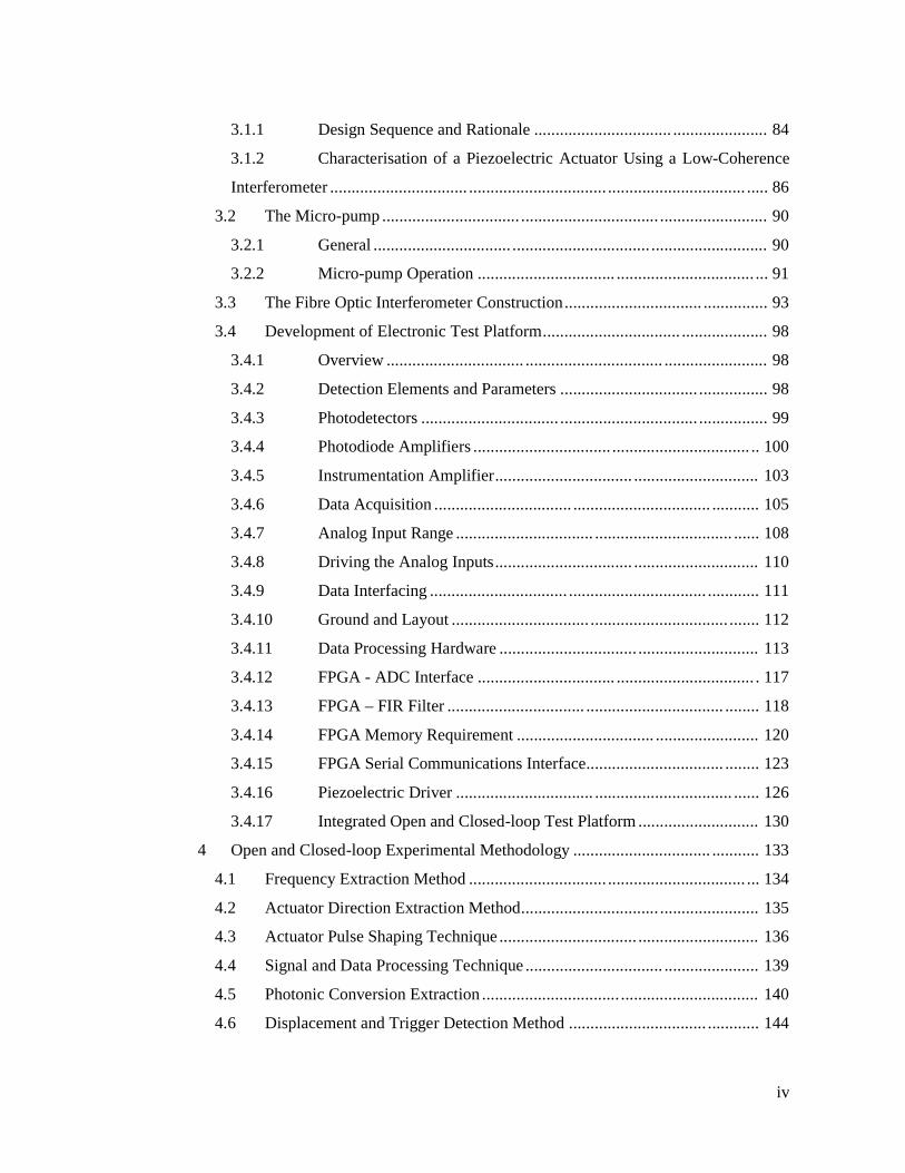
Figure 1.2 – Laboratory-on-a-Board Developed for Research Program with Micro-pump
Shown on Right (Small Coin Shown for Size Comparison)................................ ... 4
Figure 1.3 – Block Diagram of Laboratory-on-a-Board System ................................ .. 13
Figure 1.4 – Equipment Configuration for Open-Loop Characterization ..................... 15
Figure 1.5 – Schematic of Experimental Set Up for Closed-Loop System ................... 16
Figure 2.1 - Circuit Diagram for the Linear System Model (abstracted from Kim et al.,
1997) ................................ ................................ ................................ .................. 30
Figure 2.2 - Principle of the Valveless Pump Based on Liquid Viscosity (abstracted
from Matsumoto et al., 1999) ................................ ................................ .............. 37
Figure 2.3 - Cross Section of Assembled Magnetic Actuator Micro-pump (abstracted
from Khoo and Liu, 1996)................................ ................................ ................... 40
Figure 2.4 - Schematic Cut-out Illustration of a Membrane Actuator (abstracted from
Khoo and Liu, 1996) ................................ ................................ ........................... 40
Figure 2.5 - Actuation Principle of the Magnetic Membrane Actuator (abstracted from
Khoo and Liu, 1995) ................................ ................................ ........................... 41
Figure 2.6 - Layout (top view) of Permalloy Flaps (abstracted from Khoo and Liu,
1995) ................................ ................................ ................................ .................. 42
Figure 2.7 - Magnetic Actuator Testing (abstracted from Khoo and Liu, 1996) ........... 42
Figure 2.8- (a) A single crystal dipole is inherently ordered ................................ ....... 47
Figure 2.9 - Transducer configurations for use in active noise and vibration control: a)
unimorph patch PZT actuator; b) multi-layer plate-like PZT actuator; c) multi-layer
spring-like PZT actuator (n.b.: Arrows indicate direction of strain or stress.)
(Abstracted from Harrison et al., 1999). ................................ .............................. 49
Figure 2.10 - The notation of the axes for piezoelectric ceramics (abstracted from
Waanders, 1991). ................................ ................................ ................................ 50
Figure 2.11 - The Deformation of a Piezoelectric Device when Subject to an Electrical
Voltage (abstracted from Gilbertson And Busch, 1994). ................................ ...... 51
Figure 2.12 - The Bending of a Bimorph Consisting of a Piezoelectric Disc Glued on a
Membrane - Can be Used for Diaphragm Pumps (abstracted from Waanders, 1991)
................................ ................................ ................................ ........................... 52

x
Figure 2.13 - Schematic Diagram of OCT Instrumentation (abstracted from Derek et al.,
1998) ................................ ................................ ................................ .................. 54
Figure 2.14 - Schottky Barrier Photodiode (abstracted from UDT Sensors, 1982). ...... 57
Figure 2.15 - Planar Diffused Photodiode (abstracted from UDT Sensors, 1982) ....... 57
Figure 2.16 - Fibre Optic Internal Reflection (abstracted from Mercury (1992))......... 58
Figure 2.17 – Two Main Types of Fibre (abstracted from Mercury, 1992) .................. 58
Figure 2.18 – Typical Chromatic Dispersion in Single-Mode Fibre............................. 60
Figure 2.19 - Micro-pump Cross-section (abstracted from Gonzalez and Moussa, 2002)
................................ ................................ ................................ ........................... 63
Figure 2.20 - Shape of Micro-pump at a Frequency of 118 Hz (abstracted from
Gonzalez, and A. Moussa, 2002)................................ ................................ ......... 64
Figure 2.21 - Deflection of Bimorph on Actuator Side with 50V Actuation Amplitude
(abstracted from Morris and Forster, 2000) ................................ ......................... 66
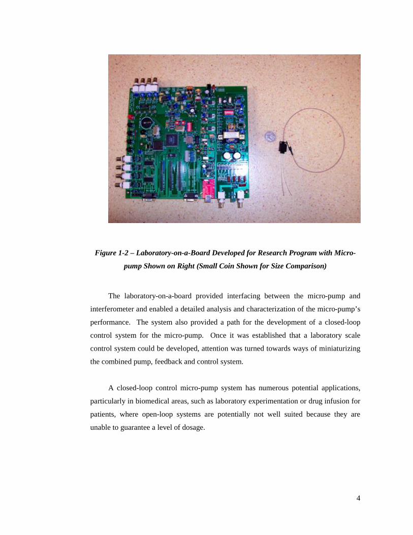
Figure 2.22 - Intensity Modulations Versus Piezoelectric Driving Voltage (graphed
from Davis et al., 2000, actual data) ................................ ................................ .... 67
Figure 2.23 - Micro-pump displacement waveforms for air, water and glycerol
(abstracted from Davis et al., 2000)................................ ................................ ..... 67
Figure 2.24 - Ringing Section of Micro-pump Displacement (abstracted from Davis et
al., 2000)................................ ................................ ................................ ............. 68
Figure 2.25 - Displacement During Pumping of Water (abstracted from Davis et al.,
2000) ................................ ................................ ................................ .................. 69
Figure 2.26 - Impulse Modulation Fringe Displacement Interpolation Process (Davis et
al., 2000)................................ ................................ ................................ ............. 69
Figure 2.27 - Schematic Diagram of Symmetric Directional Coupler (abstracted from
Trinh et al., 1995) ................................ ................................ ............................... 71
Figure 2.28 - Power Split Ratio against Coupling Length (abstracted from Trinh et al.,
1995) ................................ ................................ ................................ .................. 72
Figure 2.29 - Cascaded Directional Couplers (abstracted from Murphy et al., 1997) ... 73
Figure 2.30 - Cross Sectional Diagram Illustrating Waveguide Geometry at Point of
Closest Separation (abstracted from Murphy et al., 1997)................................ .... 74
Figure 2.31 - Measured Power Splitting Ratio vs. Wave-length for Two Cascaded
Devices (abstracted from Murphy et al., 1997) ................................ .................... 75

xi
Figure 2.32 – FCPGA plus optical assembly integration ................................ ............. 78
Figure 3.1 - Michelson Interferometer................................ ................................ ........ 86
Figure 3.2 - Optical Lever displacement sensing technique................................ ......... 88
Figure 3.3 - Self Priming Membrane Micro-pump ................................ ...................... 90
Figure 3.4 - Open-loop Fibre Optic Interferometer................................ ..................... 93
Figure 3.5 - Laser and Fibre Driving Optics ................................ ................................ 95
Figure 3.6 - Fibre and Optical Components................................ ................................ . 95
Figure 3.7 - Micro-Pump and Focusing Optics................................ ............................ 97
Figure 3.8 - Interferometer Optical Detection Closed-loop Feedback Path ................. 98
Figure 3.9 - Photodiode Modes of Operation ................................ ............................ 100
Figure 3.10 - Photodiode Amplifier and Signal Processing Block Diagram.............. 101
Figure 3.11 - Photodiode Amplifier Module and Signal Processing........................... 102
Figure 3.12 - Fringe sensing and conversion ................................ ............................. 103
Figure 3.13 - Fringe Sensing and Processing................................ ............................. 104
Figure 3.14 - Fringe Sensing and Processing................................ ............................. 104
Figure 3.15 - Sigma Delta ADC................................ ................................ ................ 106
Figure 3.16 - Digital Filter Frequency Response ................................ ....................... 107
Figure 3.17 - Frequency Response of Anti-alias Filter ................................ .............. 107
Figure 3.18 - ADC Input Block Diagram ................................ ................................ .. 108
Figure 3.19 - Bipolar (Unipolar)Mode Transfer Function................................ .......... 109
Figure 3.20 - Peak Input Signal level vs. Signal Frequency ................................ ....... 109
Figure 3.21 - Single Ended Differential Input Circuit for Bipolar mode ................... 110
Figure 3.22 - ADC Parallel Interface Connection................................ ...................... 111
Figure 3.23 - ADC Reference and Power Supply Coupling................................ ....... 112
Figure 3.24 - FPGA Data Processing Unit................................ ................................ . 113
Figure 3.25 - ACEX 1K Block Diagram (abstracted from ACEX 1K data sheet) ...... 115
Figure 3.26 - FPGA – ADC Hardware Interface Function................................ ........ 117
Figure 3.27 - Basic FIR Filter ................................ ................................ ................... 118
Figure 3.28 - Pipelined FIR Filter ................................ ................................ ............. 119
Figure 3.29 - ADC Buffer Configuration ................................ ................................ .. 121
Figure 3.30 - FIR Memory Processing ................................ ................................ ...... 121
Figure 3.31 - FPGA Internal Memory Configuration ................................ ................ 122

xii
Figure 3.32 - FPGA External Memory Configuration ................................ .............. 123
Figure 3.33 - Serial Data Transfer Interface ................................ .............................. 124
Figure 3.34 - Serial data packet configuration ................................ ........................... 125
Figure 3.35 - Piezoelectric Driver Unit ................................ ................................ ..... 126
Figure 3.36 - Integrated Piezoelectric Power Generator ................................ ............ 127
Figure 3.37 - Pulse Shaping Generator ................................ ................................ ... 127
Figure 3.38 - Pulse Driver Circuit ................................ ................................ ........... 128
Figure 3.39 - 100 V DC Amplitude shifter ................................ ................................ 128
Figure 3.40 - 20V DC Amplitude shifter................................ ................................ ... 129
Figure 3.41 - PZT Pulse Shaping Circuit................................ ................................ ... 129
Figure 3.42 - Laboratory-on-a-Board Micro-pump Characterization and Analysis
Platform Developed During the Research................................ .......................... 130
Figure 4.1 - Digitised Modulation Fringes ................................ ................................ 134
Figure 4.2 - PZT Actuation Pulse with Direction Synchronisation Slopes ................. 135
Figure 4.3 - Pulse Shaping Parameter Window ................................ ......................... 136
Figure 4.4 - PZT Actuator pulse................................ ................................ ................ 138
Figure 4.5 - Hardware based software algorithm flow diagram ................................ 139
Figure 4.6 - The dynamic Photonic conversion envelope ................................ ........ 140
Figure 4.7 - Photonic Conversion Algorithm Block diagram (Appendix B.4.2)......... 142
Figure 4.8 – Model-Sim Result for Input Modulation Using FIR Filter ..................... 143
Figure 4.9 - Trigger Detection firmware process................................ ....................... 144
Figure 4.10 - Fringe Decoder Process ................................ ................................ ....... 146
Figure 4.11 - Displacement Software Block diagram ................................ ................ 147
Figure 4.12 - Micro-pump feedback control system ................................ .................. 151
Figure 4.13 - Block Diagram of an Adaptive Micro-pump Control System ............... 153
Figure 4.14 - RC Network Circuit................................ ................................ ............. 159
Figure 4.15 - Magnitude Transfer Function................................ ............................... 160
Figure 4.16 - Phase of Transfer Function for RC Circuit of Figure 4.4 ...................... 161
Figure 4.17 - Transformation of the Control System Function................................ ... 163
Figure 4.18 - Equivalent block function ................................ ................................ .... 164
Figure 4.19 - Capacitive sensor displacement measurement set-up.......................... 168
Figure 4.20 - Average 28% glycerol displacement fringes................................ ........ 170

xiii
Figure 4.21 - First and Second-order underdamped actuator transients..................... 170
Figure 5.1 - Piezoelectric Actuator Pulse and Displacement Elicited Modulation Fringes
................................ ................................ ................................ ......................... 173
Figure 5.2 - Positive PZT Actuation and Interferometric Fringe Response ................ 174
Figure 5.3 - Digital Oscilloscope Fringe Modulation Capture ................................ .. 175
Figure 5.4 - Digitised Fringe Modulations using the DSP Algorithm ........................ 176
Figure 5.5 - Three Samples of Water Displacement Using Identical Experimental
Procedures (taken 32 cycles apart) ................................ ................................ .... 177
Figure 5.6 - Displacement when Pumping Water with 60% Glycerol ........................ 178
Figure 5.7- Three Displacement Waveforms for Water at Different Pumping
Frequencies................................ ................................ ................................ ....... 179
Figure 5.8 - Displacement Area for Samples Taken at four Frequencies.................... 180
Figure 5.9 - Plot of Flow Rate vs. Displacement and Frequency for water................. 181
Figure 5.10 - Actuator Pulse and Displacement Elicited Modulation Fringes ............ 186
Figure 5.11 - Displacement When Pumping Water (sampled every 32 periods)......... 187
Figure 5.12 - Displacement for Four Different Pumping Media................................ . 189
Figure 5.13 - Displacement for water at frequencies ranging from 10 Hz to 100 Hz . 190
Figure 5.14 - Displacement for Water at Frequencies Ranging from 10 to 100 Hz .... 191
Figure 5.15 - Area displacement modulation frequency for water.............................. 192
Figure 5.16 - Ideal Air Displacement Modulations in a 10 ms Window..................... 193
Figure 5.17 - PZT Driver Slew vs Fringes................................ ................................ . 193
Figure 5.18 - Actuator Slope Bandwidth Boundaries................................ ................. 194
Figure 5.19 - Fringe Extraction Hardware Algorithm................................ ................ 195
Figure 5.20 - Typical Fringe Extraction Timing Representation (Generated running the
waveform simulation for the circuit of Figure 5.19)................................ ........... 195
Figure 5.21 - Sum of Differentials |dv/dt| ................................ ................................ .. 196
Figure 5.22 - Audio Tweeter Displacement Based on 632.8 nm Modulation Fringes. 197
Figure 5.23 - 10 Hz Water Displacement Coefficient Generating % Variation Algorithm
................................ ................................ ................................ ......................... 198
Figure 5.24 - 10Hz Water Displacement % Variation from which the PZT Driver
Coefficients were Generated ................................ ................................ ............. 199

xiv
Figure 5.25 - Maximum Water Displacement Variations for 10Hz Excitation Frequency
................................ ................................ ................................ ......................... 200
Figure 5.26 - Moving Average Feedback Response (10 samples).............................. 201
Figure 5.27 - PZT Driver Variation from 1 – 12% and its Effect on Flow Rate for
Water at 10Hz Excitation ................................ ................................ .................. 202
Figure 5.28 - PZT Driver Variation from 1 – 12% and its Effect on Displacement and
Flow Rate for Water at 10Hz Excitation................................ ............................ 203
Figure 5.29 - Maximum Variation for Air Using Feedback Loop .............................. 203
Figure 5.30 - Flow Rate for Water using the Feedback Loop................................ ..... 205
Figure 5.31 - Maximum Displacement Variation for Each Sample Point and Range of
Frequencies................................ ................................ ................................ ....... 205
Figure 5.32 - Maximum Displacement Closed-loop Response Variations ................. 206
Figure 5.33 - Closed-loop Flow Rate Analysis Using Three Media (water, water+28%
and 60% glycerol) ................................ ................ Error! Bookmark not defined.
Figure 6.1 - Percentage Variation for the Displacement Plotted for Open and Closed-
loop Data Sampled for 60 seconds at 10 Hz................................. ...................... 210
Figure 6.2 - Plot of Point-to-Point Displacement Variation for the Open-loop and
Closed-loop Comparison extracted from Tables 5.2 and 5.4 .............................. 210
Figure 6.3 - Trigger Window for Closed-loop Operation Initialisation ...................... 212
Figure 6.4 - Polymer Optics Planar Wave-guide Channelling................................ .... 215
Figure 6.5 - Cross Section of a Fully Integrated System................................ ........... 217

xv
Table of Equations
Equation 1 APWcdtkdt
dWcmkfeV ∫ ++= γ ................................ ..... 29
Equation 2 Pcdt
dQcIcP += ................................ ................................ 29
Equation 3 ∫ −−= QodtQiQcCc
Pc 1................................ ................... 30
Equation 4 dtQCDt
dQIIQRRP ot
otvotvc ∫++++=
1)()( ................................ .... 30
Equation 5 drrrr
Amassactualmasseffective
o
+== ∫
ππγ cos1
22
__
.................... 31
Equation 6 ( ) ( )membraneactualPZTactual ymmm += γ ................................ ................ 31
Equation 7 ghouvc
c CnPV
KAhC a
sin++= ................................ .................... 31
Equation 8 AhI c
cρ
= ................................ ................................ .... 32
Equation 9 ( ) ( )∫
+== dx
xwxhdLR
vvHv
4
4
118128πµ
πµ ................................ ....... 32
Equation 10 ( ) ( )∫=xwxh
dxIvv
v ρ ................................ ................................ 32
Equation 11 VW
f acc ω
= ................................ ................................ ................ 32
Equation 12 ( )wa
w
cc
c
WWAP
k−
=γω
................................ ................................ 33
Equation 13 wcc
c WPAC
ωγ
= ................................ ................................ ....... 33
Equation 14 2n
kmω
= ................................ ................................ ............... 34

xvi
Equation 15 222
2
Am
ACAk
In
cc −
+=
ω................................ ................................ .. 34
Equation 16 QPR v
∆= ................................ ................................ ............. 34
Equation 17 lEdll
UdUdl ∗∗=∗∗=∗=∆ 333333 ................................ .......... 51
Equation 18 aEdal
UdUda ∗∗=∗∗=∗=∆ 313131 ................................ ........ 51
Equation 19 S = cos2 θ sin2(Ф 1 + Ф 2) + sin2 θ sin2(Ф 1 _ Ф 2) ..................... 73
Equation 20
−=
+=
NN11
83,11
83
21
ππ φφ ...................... 73
Equation 21 1
2
23sin
23sincos
−
+
=
NN
Nππ
θ ................... 73
Equation 22 Ф1 = π/2, Ф2 = π/4, and θ = π/3................................. ..................... 74
Equation 23 ,2 xf
bw CRfuf
π= (where Cx = Cj + Cin) ................................ ..... 102
Equation 24 ∑=
=8
1)(*)()(
nnhnxny ................................ ................................ . 118
Equation 25 tfd m
A∆
∝∆ ................................ ................................ .............. 134
Equation 26 12 mm kff = ................................ ................................ ................. 134
Equation 27 λ×= −−
T
tTnf C
CD )(
)1( ................................ ................................ ..... 146
Equation 28 i
o
VVfG =)( ................................ ................................ ................. 159
Equation 29 ( )ee ftiftiin i
AtV )2(2
2)( ππ −−= ................................ ............... 162
Equation 30 ee ftiftiout fG
iAfG
iAtV )2(2 )(
2)(
2)( ππ −−−= ........................... 162

xvii
Equation 31 ee fGftifGftiout fG
iAfG
iAtV ))((2())((2 )(
2|)(|
2)( ∠−−∠+ −−= ππ
.. 162
Equation 32 )sin()( φω += ttf ................................ ................................ ...... 164
Equation 33 22
cossin)(ω
φωφ++
=s
ssF ................................ ............................. 164
Equation 34 ∑ ∫−
=N
tn
1tn
udtArea ................................ ................................ ......... 167
Equation 35 ( )( )2
ttuuttuf(t) n1)(nn1)(nn1)(nn
n −−+−=
++
+ ............................... 167
Equation 36 tAe ατ −= ................................ ................................ ................... 169
Equation 37 tAe dt ωτ α sin−= ................................ ................................ ....... 169
Equation 38 tet dt
d
ωω
ω α sin1)( −= ................................ ................................ 169
Equation 39 ( )fAAxf xx **2sin)( π= ................................ ................. 191

xviii
List of Acronyms and Abbreviations
AC - Alternating Current
ADC - Analog-To-Digital Converter
AGC - Automatic Gain Control
BS - Beam-Splitter
CIU - Communication Interface Unit
CMOS - Complementary Metal-Oxide Semiconductor
CPLD - Complex Programmable Logic Array
CPU - Central Processing Unit
CRC - Cyclic Redundancy Check
CVC - Current-To-Voltage Converter
DAC - Digital-To-Analog Converter
DC - Direct Current
DSP - Digital Signal Processing
EAB - Embedded Array Block
FCPGA - Flip-Chip Pin Grid Array
FEC - Forward Error Correction
FIR - Finite Impulse Response
FOC - Fibre Optic Converter
FPGA - Field Programmable Gate Array
IC - Integrated Circuit
ICPF - Ionic Conducting Polymer Film
IOE - Input Output Elements
IP - Intellectual Property

xix
ISP - In-System-Programmable
JFET - Junction Field Effect Transistor
LAB - Logic Array Block
LED - Light Emitting Diode
LIU - Line Interface Unit
LSB - Least Significant Bit
LUT - Look-Up-Table
MEMS - Micro Electro Mechanical Systems
MSB - Most Significant Bit
MT - Multi-Terminal
NMP - No-Moving-Parts
OSR - Over-Sampling Ratio
PA - Piezo-Actuator
PC - Personal Computer
PD - Photo-Detector
PDMS - Polydimethyl Siloxane
PLL - Phase Locked Loop
PROM - Programmable Read Only Memory
PWM - Pulse Width Modulation
PZT - Piezoelectric Transducer
RAM - Random Access Memory
RIE - Reactive Ion Etching
RM - Reference Mirror
SMF - Single-Mode Fibre

xx
SNR - Signal-To-Noise Ratio
SOI - Silicon-On-Insulator
SOPC - System-On-A-Programmable Chip
SPI - Serial Peripheral Interface
TCA - Trans-Conductance Amplifier
VHDL - Very High-level Design Language
VLSI - Very Large Scale Integration
WDM - Wavelength-Division-Multiplexed

xxi
Abstract
This thesis constitutes the documentation for a Doctoral research program
undertaken at the Industrial Research Institute of Swinburne University of Technology
(IRIS) between 2001 and 2005. The focus of the research was an investigation of the
open- and closed-loop response of piezoelectric micro-pumps for micro-fluidic
applications, particularly for chemical and biomedical environments. Specifically, in
order to successfully integrate micro-devices into functional systems, it was important
to address issues of real-time performance monitoring and control. The research
addresses some of these problems in the context of a piezoelectric-driven micro-pump,
equipped with interferometric displacement feedback, which was used to measure the
dynamic displacement of the micro-pump actuator surface.
During the course of the research, both a discrete component and a fully integrated
(laboratory-on-a-board) test system were developed for open-loop characterization of
the micro-pump. The laboratory-on-a-board system was also used for closed-loop
control application. Measurements showed significant differences in actuator velocity,
displacement and settling time between different pumping media. In addition, transient
underdamped vibration of the actuator surface was observed during the rapid excursion
and recursion phases of the pump movement while pumping air. These non-contact
measurements could be used to determine the open-loop characteristics of a micro-
pump and provide information for design improvement or failure detection/analysis.
The technique could also be used to provide continuous measurement for adaptive
compensation, so that the pump performance criteria are always satisfied. To this end,
an automated interference fringe counting algorithm was developed, so that the steady-
state parameters could be mapped into the closed-loop control elements in real time.
The performance of this algorithm is discussed herein, together with the implications for
optimal control of the micro-pump, and eventual integration of the interferometer and
micro-pump systems. The research indicated that there were potential benefits in
closed-loop control of micro-pumps, particularly where failure detection was required
and for pumping of non-homogeneous media. The thesis also documents the relative
performance differences between open and closed-loop control in homogenous media.

1
1 Introduction

2
1.1 Overview
This dissertation provides the documentation for a Doctoral research program
conducted in the field of micro-pump feedback and control. The research was
undertaken at the Industrial Research Institute of the Swinburne University of
Technology (IRIS) in Melbourne Australia between the years of 2001 and 2005.
The objective of the research was to investigate and characterise the open-loop
performance of an important micro-electro-mechanical system (MEMS) component,
specifically a piezoelectric micro-pump, and then to develop a closed-loop control
system for the pump. Two of the key issues in the control regime were:
• To identify potential causes (signals) of failure in the micro-pump
• To provide a system that could optimise for parametric limitations in
both the electrical and mechanical elements of the pump and to
account for variations in non-homogeneous pumping media.
The principal feedback mechanism that was investigated for the purposes of this
research was a fibre-optic based interferometer system. Another follow-on aspect of the
research was therefore to investigate whether the closed-loop micro-pump control
system could be integrated into a small package system (i.e., of a size comparable to the
micro-pump itself) that could have potential commercial applications.
In terms of developing a feedback system for a micro-pump, it was imperative
that any measuring system, which arose from the research, could be integrated without
impeding the performance of the pump. A typical micro-pump, such as the one that was
used as the basis for this research, is shown schematically in Figure 1.1.

3
Figure 1-1 – Schematic Diagram of Piezoelectric Micro-pump
This dissertation describes the research undertaken in applying a non-contact,
fibre-optic-based interferometer for measuring the dynamic displacement of a micro-
pump, as a measure of fluid flow feedback. This technique was applied externally to
the MEMS structure. The feedback approach was selected so that the optimum
displacement of the piezoelectric actuator membrane could be maintained for any given
gas or liquid being pumped through the micro-pump valves and chambers.
In order to facilitate an investigation of the efficacy of the interferometer as a
feedback device, a comprehensive laboratory system had to be designed, developed and
implemented during the course of the Doctoral research. The first stage involved the
development of a discrete component system for open-loop characterisation. The
second stage involved the development of a more sophisticated (laboratory-on-a-board)
integrated system that could provide a basis for both open and closed-loop control. The
integrated system is shown in Figure 1.2.
Pump chamber
Outlet valve
Piezoelectric actuator
Diaphragm
Solid substrate layers
PZT electrode (+)
PZT electrode (-)
Outlet Inlet
Valve membrane
Inlet Valve
4
Figure 1-2 – Laboratory-on-a-Board Developed for Research Program with Micro-
pump Shown on Right (Small Coin Shown for Size Comparison)
The laboratory-on-a-board provided interfacing between the micro-pump and
interferometer and enabled a detailed analysis and characterization of the micro-pump’s
performance. The system also provided a path for the development of a closed-loop
control system for the micro-pump. Once it was established that a laboratory scale
control system could be developed, attention was turned towards ways of miniaturizing
the combined pump, feedback and control system.
A closed-loop control micro-pump system has numerous potential applications,
particularly in biomedical areas, such as laboratory experimentation or drug infusion for
patients, where open-loop systems are potentially not well suited because they are
unable to guarantee a level of dosage.

5
1.2 Background
MEMS technology is well suited to the fabrication and integration of micro-
fluidic systems, which offer a novel solution to chemical and biochemical analysis and
synthesis. The integrated micro-fluidic systems may be constructed from any number
of micro-fluidic components and upon a regular circuit substrate. There are many
benefits in miniaturization of these biomedical systems, including substantial savings in
the time taken to perform laboratory analysis; the cost of analysis, and space utilization
for the equipment performing the analysis. Ultimately, it is desirable to provide systems
capable of performing a variety of different fluidic operations integrated in a single
system (Forster et al., 1995). To achieve this, it is imperative that reliable and accurate
monitoring and control of the parameters for any of the fluidic elements within the
micro-fluidic system be implemented.
Typically, a micro-system is composed of devices categorised as micro-sensors or
detectors (which detect any changes within the system environment); intelligent
electronics capable of making decisions based on the changes indicated by the sensors,
and micro-actuators capable of altering the system environment according to the
directives from the intelligent electronics.
Micro-fluidic systems are emerging not necessarily from the industrial demand
but from the technologies that enable the fabrication of such micro-components (Forster
et al,, 1995). The application targets for a micro-pump range from medical, biological,
pharmaceutical to chemical where miniaturization increases portability; reduces cost;
increases accuracy; reduces the amount of chemical or biological samples required for
analysis, and also reduce measurement time.
A reduction in size, however, also implies a reduction in quantity, so micro based
processing plants are best suited for distributed processing of materials at the immediate
point-of-use. In biomedical applications, an implantable micro-pump can be fabricated

6
to accurately, and on demand, administer the amount of pharmaceutical product
required, because flow rates can be controlled precisely by the integrated electronics.
A number of micro-pumps are fabricated based on piezoelectric membrane
actuators. However, at the time this research program commenced, many of the
piezoelectric actuator membrane displacement measurements were implemented using
non-contact pressure sensors or optical lever fibre-optic techniques. The technique
described in this dissertation, however, is particularly novel in its application to micro-
pumps, because it incorporates a precise approach to sensing which integrates an
elaborate network of optical components, such as directional couplers,
collimating/focusing lenses and shorter lengths of single mode fibre.
Numerous papers have been published (detailed in the literature review of this
thesis) that investigate the properties of piezoelectric materials and their behaviour
when stimulated with a specific potential. There have also been numerous papers on the
subject of micro-pump construction techniques, based upon the no-moving-parts (NMP)
concept, and characterised using simulation models.
The reviewed literature suggested that micro-pump characterization was typically
performed on a free running open-loop experimental methodology, producing a set of
test results that did not allow for variation in the controlling elements of the system,
particularly when variations within the media, such as viscosity, temperature and
impurities were introduced into the pump. This potentially led to large percentage
errors in dosage, and decreases in the performance and reliability of micro-pumps, but
also presented a new set of challenges that were addressed in this Doctoral research.
This dissertation will present results which indicate that by monitoring the
mechanical performance of the micro-pump, it is possible to make adjustments, in real-
time, to a number of controlling elements by way of compensation using a closed-loop
approach. At the time this research commenced, a closed-loop approach was typically
applied by monitoring the volume of the medium being displaced (by continuously
measuring the amount remaining, knowing the initial amount). This approach,

7
however, only indicated that there were variations during pumping, which could not be
mapped to any of the structural parameters, and therefore eliminated any possibility for
adaptive compensation.
In terms of the devices themselves, it needs to be noted that mechanical micro-
fluidic handling systems are composed of micro-pumps and micro-valves, which
employ various actuation mechanisms (Zhang et al., 1996, p.94−97). The actuation
principles that have been applied to membrane micro-pumps include:
• Piezoelectric (Koch et al., 1998)
• Electrostatic (Zerlenge et al., 1992)
• Thermopneumatic (Jeong et al., 1999)
• Bimetallic (Yang et al., 1995)
• Electromagnetic (Zhang et al., 1996)
The membrane material chosen for these devices is generally silicon (Koch et al,
1998). The types of micro-valves and flow controllers used include:
• Passive check valves (Zerlenge et al., 1992)
• Active diaphragm valves (Zhang et al., 1996)
• Nozzlediffuser pairs (Koch et al., 1998).
For many electrostatic and piezoelectric membrane actuators, large actuation
voltages are required. For example, the PZT actuator for a micro-pump discussed by
(Koch et al., 1998) required a 600 Vpp driving voltage.
Since the achievable displacement for flat-membrane actuators is generally
limited (from a few microns to 10−20µm), the overall volume flow rate of micro
membrane pumps is thereby limited as well. To achieve larger deflections, novel
structured membranes, such as corrugated membranes (Jeong et al., 1999) have been
fabricated, although these require a more involved fabrication process. Jeong et al.
compared deflections for flat and corrugated silicon diaphragms of the same

8
dimensions. A 4 × 4 mm2 membrane, with 7 corrugation rings, deflected by 37.5-µm
while a flat membrane only yielded an 11.7-µm deflection under a 6V applied voltage.
Alternately, elastic materials such as silicone elastomers (Bieider et al., 1995) are used
for their low Young’s Modulus. This means that larger membrane displacements are
achievable with similar power inputs. Larger displacements in the actuators translate
into larger stroke volumes and higher flow rates in the micro-pump. Besides their
favourable mechanical properties, silicone elastomers are physically and chemically
stable and inert, thus making them biocompatible.
Magnetic actuation (Sadler et al., 1998) had also been explored for its favourable
characteristics. It was shown to produce large forces (a few hundred µN), which
effected large displacements. Many of these micro-pumps and micro-valves were
driven by integrated magnetization sources, which required wire feed. A group that
explored magnetic effects as an actuation principle, Zhang et al., (1996), fabricated a
magnetic membrane micro-pump with a 7-µm thick Permalloy film on a 17-µm-thick,
8× 8 mm2 silicon membrane. This membrane achieved 23-µm deflections when driven
by integrated inductors operating at 300 mA DC and 3 V. The novel aspect of this work
was the fabrication of the first tether-less micro-machined membrane pump, based on
polymer material and external magnetic actuation.
In comparison, the membrane on the micro-pump in this research was four times
smaller than the one reported by Zhang et al. (1996) and achieved four times greater
displacement. In the micro-pump used by Zhang et al. (1996), the actuation force was
provided by an external magnetic field (for which great flexibility was given to its
positioning), and the device could be remotely operated without needing any wires for
power input to the device. It was also known that material damage was not a concern
under high magnetic fields up to one Tesla (Liu, 1998). Testing of the device was
performed at low fields of 0.11 to 0.23 Tesla, which was sufficient to produce the large
displacements and thus the flow rates measured.

9
1.3 Central Research Theme
The central theme of this research was the investigation of feedback and control
systems application to micro-systems, specifically a micro-pump. A key issue here was
that conventional feedback and control systems did not necessarily translate well into
the micro-system domain. Numerous factors came into play in terms of the
characteristics and performance of such systems (Gerlach et al., 1995), and hence there
was a need to investigate a range of problems in order to understand the methods and
technologies that would be required to produce viable systems.
The Doctoral research program was therefore composed of several major elements
which are summarised as follows:
(i) Investigation of an accurate and reliable non-contact measuring instrument
(specifically an interferometer) to be used as a sensor for the
electromechanical characterization of an open-loop piezoelectric-driven
micro-pump.
(ii) Design, development and implementation of two experimental platforms to
facilitate experimentation – the first being a discrete component system for
open-loop characterisation of the pump, and the second being a more
comprehensive laboratory-on-a-board system that could be used as a tool for
detailed experimentation into feedback and control of micro-pumps.
(iii) Investigation of the control for the micro-actuator, using intelligent
electronic microcircuits suited to the development of an efficient and
reliable adaptive micro-controller. Specifically, the controller had to
achieve real-time closed-loop performance and, importantly, the chosen
techniques had to be suitable for ultimate integration into the micro-pump.
In other words, there had to be a focus on the total micro-system integration.

10
Moreover, having achieved a closed-loop control system for the micro-pump, the
subsequent objective was to compare the closed and open-loop performance to
determine whether there was a benefit in providing closed-loop control in the first
instance.
The ultimate outcome of the research was to determine whether an adaptive and
reliable piezoelectric driven micro-pump could be developed for use in a variety of
micro-fluidic systems, particularly medical drug delivery; chemical and medical
diagnostics; ink-jet printers, as well as any devices requiring transference of liquids or
gases. The investigation therefore also included a study of the following elements that
would be required for micro-fabrication of the integrated, closed-loop system,
specifically:
• Micro-fabrication techniques (e.g., photolithography, laser ablation, wet
chemical etching, air abrasion, embossing, injection moulding and
others).
• Substrate material selection according to tolerance, and with exposure to
conditions such as extremes of pH, temperature, salt concentrations,
chemical abrasions and electric fields.
• Substrate materials with preferred aspects associated with the
semiconductor fabrication, including silica based substrates, quartz, poly-
silicon, glass, gallium arsenide and others.
• Application specific micro-fluidic system integration techniques based
on the adaptive closed-loop microelectronic monitoring and control
logic, characterised for a generic piezoelectric-driven micro-pump.
A comprehensive study of the earlier attempts to develop micro-pumps within
micro-fluidic systems identified a number of areas requiring further research in order to
improve their performance and reliability. Numerous tests and procedures were

11
therefore developed for the dynamic measurement of micro-pumps in order to
characterise their performance. The most effective measurements for the MEMS
structures, without impeding their performance, were achieved by the use of non-
contact sensing techniques. A key thrust of this research was therefore meeting the
objective of a non-contact feedback device that lent itself to subsequent micro-
fabrication.

12
1.4 Overview of Methodology
The research program had two major components – the first being a
characterization of a micro-pump and the second being the implementation and testing
of the closed-loop control system. Each of these elements had sub-components and,
hence, the basic steps involved in the overall research were as follows:
• Development of experimental system (discrete component system) to
provide a testing platform for characterisation of micro-pumps
• Implementation of fibre optic feedback device
• Analysis and characterisation of micro-pump in open and closed-loop
configurations
• Development of a comprehensive (laboratory-on-a-board) system for
closed-loop control, and implementation of closed-loop algorithms
• Testing and performance evaluation of closed-loop control system
• Investigation of micro-system fabrication and integration issues.
The development of the laboratory-on-a-board was a significant component of the
research because it provided a purpose-designed platform on which to conduct the
overall experimentation program. The laboratory-on-a-board system also provided a
means of verifying the results obtained with the original, discrete-component system.

13
1.5 Overview of Experimental Procedures
1.5.1 Development of Laboratory-on-a-Board
A key element of the research program was the development of a laboratory
experimental system that would facilitate the characterization of a micro-pump system,
which would also enable development, implementation and testing of closed-loop
algorithms. The Laboratory-on-a-Board system is shown as a block diagram in Figure
1.3.
Figure 1-3 – Block Diagram of Laboratory-on-a-Board System
The key elements of the Laboratory-on-a-Board System that was developed for
the purposes of this research were:
Process and Control Electronics Fibre O ptic
Converter (FOC)
Analog to Digital
Converter (ADC)
Adaptive
Compensation Driver
Micropump
Actuator Driver
Data
framing
CPU
Memory Management Unit
Flas h DPRA M
FI F O
Timin g Control
SPI
PWM Gen.
FEC Gen.
Communication Interface
Digital to Analog
Converter (DAC)
PZT Voltage Generator
Programm ing Controller
Debugging
Monitor
Serial Controller
Fibre Optic Interferometer
Fibre PZT Stretcher
Micropump Actuator
PC

14
• Fibre Optic and the Analog to Digital Converter
Utilising high sensitivity photodiodes, wide-band trans-conductance
amplifiers and high speed analog to digital converters
• PZT Controller Driver
Incorporating phase shifters, frequency modulators, high voltage generators
and amplitude controllers
• Hardware Processing and Analysis Platform (CPU/FPGA)
Mass storage, data filtering, data framing, data conversion and arithmetic
processing
• Communications Interface Unit (CIU)
Serial data transfers, configuration and system monitoring
1.5.2 Micro-pump Characterisation
The aim of the characterisation phase of the research was to use the results from
the work by Davis (1999), as the basis for the development of an efficient and reliable
fibre optic interferometer feedback system for a micro-pump requiring high linearity,
long term position stability, repeatability and accuracy.
The experimental configuration for the open-loop micro-pump characterization is
shown schematically in Figure 1.4, which utilises a discrete test platform further
described in Chapter 3. The arrangement was composed of a micro-pump, secured on a
vertically mounted base (targeted using a horizontally positioned focusing adjustable
lens), fibre optic interferometer, detection electronics, data acquisition and processing
hardware (laboratory-on-a-board), monitoring instruments and an embedded micro-
controller for data analysis.

15
Figure 1-4 – Equipment Configuration for Open-Loop Characterization
The characterization of the micro-pump served as the basis of the performance
and reliability measurement. The open-loop analysis was used to generate the data used
to characterise the steady-state response of the system, based on the frequency and
amplitude variations for a given pumping medium. The micro-pump response was
measured for:
• Frequencies ranging from 2 Hz to 100 Hz
• Amplitude variations between 100V and 400V DC
• Pumping media such as air, as well as varying percentages of Glycerol and
water.
The displacement analysis was processed using discrete and digital-hardware-
generated mathematical algorithms and the results tabulated.
Laboratory-on-a-Board Fibre Optic
Interferometer With Laser
Driver
Micro-pump
Amplifier ADC
PZT Driver
Data
Acquisition & Analysis
PZT Controller
PC Interface DAC
Oscilloscope
PC

16
1.5.3 Closed-loop Control
The data obtained from the open-loop analysis described in 1.5.2 was applied in
order to undertake closed-loop experimentation. This generated a set of error
coefficients, based on continuous real-time complex transfer functions, which were then
applied in a feedback control loop using an embedded (and hardware generated)
adaptive algorithm. The closed-loop experimental configuration is shown in Figure 1.5.
Figure 1-5 – Schematic of Experimental Set Up for Closed-Loop System
The experimental set up for closed-loop is composed of the same elements as the
open-loop system but with closed-loop control electronics added. These include an
actuation pulse generator, frequency and phase controller, monitoring instruments and
an embedded micro-controller for data analysis. The laboratory-on-a-board system was
designed for the purposes of carrying out the open and closed-loop analysis as well as
the control for the micro-pump.
Laboratory-on-a-Board Fibre Optic
Interferometer With Laser
Driver
Micro-
Amplifier ADC
PZT Driver
Data
Acquisition & Analysis
PZT Controller
PC Interface DAC
Oscilloscope
PC
Feed
back
C
ontr
olle
r

17
The complexity, the cost and size of the experimental platform demonstrated the
requirements for a smaller and more compact system that could be integrated into the
micro-pump in order to make this an economically and technologically viable option for
commercialisation.
It was intended that the displacement measurement of a micro-pump actuation
membrane be continuously monitored for variations in frequency and amplitude. Any
deviations on a cycle-to-cycle basis were mapped as compensation for the loss or gain
of the system, thereby enabling optimum efficiency, performance and reliability to be
maintained.
The error was accumulated using a moving average function and compared with
normalised open-loop tabulated data for a given pumping medium. If the error exceeded
0.1% (over a complete cycle), an adaptive algorithm was enabled and the error adjusted
accordingly over the next actuating cycle. The compensation was in the form of
frequency or amplitude variation, based on the forward error correction percentage that
incorporated previous error coefficients with the normalised expected tabulated data.
1.5.4 Integration Considerations
This element of the research incorporated a number of disciplines, such as
microelectronics, polymer based optics and micro-electro-mechanics. The data
accumulated during the open- and closed-loop phases of the research, and subsequent
analysis, highlighted the need for the integration of polymer based optics with the
micro-pump and the microelectronics into a single compact unit which would need to be
similar in size to currently available commercial micro-pumps.
This phase of the research investigated the processes and techniques that could
be applied to achieve the intended integration. The experimental platform for the
integrated system was composed of:
• A full polymer-based optic design (modelled through simulation)

18
• A micro-pump as characterised earlier in the research
• Microelectronic design based on the control electronics test platform
defined in the closed-loop phase of the research.
The microelectronics section was modelled using circuit simulations, as it was
not possible to take the design through its fabrication process.

19
1.6 Perceived Contributions
During the course of the research, it was established that a fibre optic
interferometer could be an effective and accurate instrument for measuring the
displacement of a micro-pump actuation membrane. The elicited modulation fringes
generated by the movement action of the actuator are directly proportional to the
velocity and the wavelength of the infrared laser source, which in turn, translates into
the displacement of the piezoelectric actuator membrane. The non-contact feedback
approach investigated in this research program does not impede the performance of a
micro-pump, unlike capacitive, resistive, pressure and thermal based sensors that rely on
contact in order to elicit an interactive response.
Following on from the characterization of micro-pump performance, the fibre-
optic interferometer was found to be a novel way of ensuring that accuracy, reliability
and performance could be maintained through closed-loop control. Prior to the
commencement of this research, micro-pumps were generally free-running devices,
without direct structural monitoring. This necessitated a complex and technically
challenging approach to be applied to the whole micro-fluidic system in order to
determine the accuracy and performance characteristics of a pump. On the other hand,
having a micro-pump capable of monitoring and controlling its own structural integrity
(independently) potentially facilitates:
• A greater level of integration
• Size reduction
• Improved efficiency
when used in a micro-fluidic system, particularly where the pumping medium is non-
homogeneous.

20
Based upon the above discussions, the specific contributions of this research were
identified as follows:
• A comprehensive review of research in the field of micro-pumps, potential
feedback devices, control strategies and available integration technologies
• The design and development of electronics (both a discrete component
system and integrated, laboratory-on-a-board) capable of processing
interferometric information and analysing and controlling micro-pump
structural characteristics.
• The design and development of a fibre optic interferometric sensing
instrument for measuring displacement of a piezoelectrically driven
actuation membrane in a micro-pump.
• Development and implementation of a comprehensive closed-loop control
system
• Investigation, analysis and proposal for the design and development of
fully integrated polymer based optic interferometer with microelectronics
fabrication on a polycarbonate structure of a micro-pump.
The research documented in this thesis was also published in a research paper:
Tomac, T., Wheeler, K., Colonna, A., Stoddart, P. and Mazzolini, A., “MEMS
Micro-pump Characterization and Control Utilizing a Fibre Optic Interferometer”,
Proceedings of SPIE -- Volume 4935, Published on-line, 2003

21
1.7 Thesis Structure
This thesis is composed of six chapters, five of which follow on from this
introduction. Specifically, the chapters are summarised as follows:
• Chapter 2 presents a detailed literature review that provides the impetus for
the various strategies adopted during the course of this Doctoral research
• Chapter 3 presents the details for the design and construction of the open
and closed-loop test platform
• Chapter 4 discusses the open and closed-loop experimental configurations
and methodology.
• Chapter 5 presents the open and closed-loop experimental results based on
the experimental test platform defined in chapter three.
• Chapter 6 presents open and closed-loop comparison analysis.
• Chapter 7 envelopes a broad-context discussion based on the outcomes of
this research.
• Chapter 8 presents conclusions and recommendations

22
2 Literature Review

23
2.1 Overview of Review Process
The literature review in this Doctoral research was conducted through various
electronic media and through library catalogues, references to patents, journals, books,
conference and research papers.
The electronic media proved particularly useful in extracting abstracts from
patents and journals, and facilitated identification of key points relating to the central
research theme. In particular, the categorised, searchable, directory of search engines
(located at web address http://www.searchengineguide.com/searchengines.html) proved
to be a valuable resource and offered topical search engines, portals, and directories on a
wide variety of relevant topics. Other databases and resources that were employed as
the basis of this literature review included:
• EBSCOhost - a collection of databases, many including full text articles
found in articles and journals
• OVID database - from the Institute for Scientific Information, provided
access to the tables of contents and bibliographic records with abstracts for
more than 8,000 international scholarly journals covering many academic
disciplines.
• Delphion database - provided a comprehensive intellectual asset
management (IAM) software and service. Delphion provided access to
research, IP management and analytic tools
• The US patent website http://www.uspto.gov/ - provided access to all
patents registered over the past ten years. This was useful in identifying
current technological trends.

24
• ISI Web of Knowledge/Web of Science – General academic search tool for
research literature and citation checks.
• Scopus – Academic publications related to engineering and applied science
disciplines.
The literature review presented in this chapter covers the following topics:
(i) A historical perspective on micro-pump systems
(ii) Design, modelling and testing of micro-pumps
(iii) Actuation of Micro-pumps, including the magnetic membrane pump
actuator
(iv) Piezoelectric Characterisation
(v) Optimisation of piezoelectric diaphragms
(vi) Piezoelectric ceramics as in-plane actuators
(vii) Piezoelectric actuators having stable resonant frequency
(viii) Characterisation of piezoelectric actuators using low coherence
interferometer
(ix) Optical coherence tomography
(x) Photodiodes
(xi) Fibre optics
(xii) Open-loop characterisation of micro-pumps
(xiii) Closed-loop control of micro-pumps.
At the end of the chapter, the findings of the review, and the research directions arising
from it, are summarised.

25
2.2 A Historical Perspective on Micro-Pump Systems
Initial fabrication of micro-mechanical components was achieved through the
use of etching processes and, when applied to bulk silicon substrates, any number of
very complex geometric shapes could be generated. This was the beginning of micro
machining in the early 1980s that evolved the fabrication processes for the development
of the micro-mechanical components and associated elements e.g., pressure sensor
diaphragm and cantilever beam for accelerometers.
Finne and Klein (1967) and also Price (1973) were instrumental in using the
anisotropic etching of silicon for fabrication of transistors whereas, in the 1960s,
isotropic etching had been used. This led to development of a number of etch-stop
techniques that provided additional flexibility and further enhanced and expanded the
techniques for fashioning of micro-mechanical components from silicon substrates.
These became known as “bulk” micro machining.
Early limitations, combined with increasing demand for design flexibility, better
performance and greater reliability, led to innovations in micro machining. The
sacrificial layer and surface micro machining techniques emerged in the mid 1980s,
which allowed for fabrication of numerous types of micro mechanical elements and
components, while the silicon substrate acted only as a mechanical support.
In subsequent developments, chemical silicon fusion bonding and high-aspect
ratio lithography, along with plating processes, were introduced and these further
expanded the capabilities of micro machining technology. The techniques for integrated
fabrication of mechanical structures (formed from rigid bodied elements connected
together by joints) were developed in the late 1980s (Mehregany et al., 1988). This
showed that unrestrained motion of mechanical parts could be executed to at least one
degree of freedom (e.g., gears, linkages, levers, etc.). This led to the development of
electrostatic micro-motors and other types of micro-actuators, such as valves, switches,
piezoelectric pumps and resonant devices.

26
Progress in micro-actuators transformed the conventional field of solid-state
transducers into what became known as micro-electro-mechanical-systems (MEMS).
MEMS evolved in 1987/1988 with the formation of a number of workshops on Micro-
dynamics and MEMS at Salt Lake City (Utah); Hyannis (Massachusetts), and at
Princeton (New Jersey), thereby leading into a new era of micro-devices.
Miniaturization of mechanical systems had the potential to provide smaller,
lighter, faster and more precise devices. However, these required appropriate
fabrication techniques, allowing for: small geometries; precise control; design
flexibility; control electronics interfacing; reliability, and a very high yield, while
retaining a low cost per device. Micro-fabrication was a primary source for the
development of micro-mechanical systems, and it facilitated integration of micro-
mechanical systems with electronics, thereby facilitating the development of high-
performance closed-loop control MEMS. Generally, MEMS integration of micro-
sensors, micro-actuators and electronics into the same environment was made possible
because the need for discrete component assembly could be eliminated through the
application of complementary fabrication techniques.
Micro-pumps evolved from the advent of MEMS technology. Positive-
displacement micro-pumps are mechanical structures that are composed of a membrane
or a diaphragm displaced by an actuator, which is driven piezoelectrically, magnetically
or by any number of well-established stimuli. Architecturally, these are formed over a
chamber connected by unidirectional inlet and outlet valves, and were first developed in
the early 1990s. A number of micro-pumps with piezoelectric actuators of varying
driving voltages (50V – 400V), utilizing no-moving-parts (NMP) valves, were
fabricated in the mid 1990s (Gerlach and Wurmus, 1995).
At the time this Doctoral research commenced, micro-pumps relied upon natural
resonance for optimum performance in an open-loop configuration. Controlled closed-
loop systems were reliant on external sensors, such as thermocouples; magnetic wafers,
pressure sensors and multiple microelements that needed to be added in order to

27
successfully control the actuation and subsequently the flow rate. This generally meant
that the complete systems were too bulky for human implantation and so, many such
systems were applied externally. Ultimately, it was believed that a controlled drug
delivery system would be developed, based on the MEMS structures, that were safe,
reliable and small enough for implantation.
Implantable micro-pump systems had to be able to provide well-controlled
release of pharmacological agents. More importantly, site-specific targeted drug
delivery also had the potential to lower the dose that needed to be administered to
patients. Hence, a controlled closed-loop system was ideal, since it could incorporate
any number of chemical sensors that could react with the levels of blood agents and
subsequently control dosages for patient administration.
The Sensors and Actuators journal was published in 1980 with an objective to
establish a forum towards inviting for publication of research papers within the field. In
1989, MYU Publishing Japan also released a journal, Sensors and Materials. Since
then, many publications dealing with actuator, sensors and micro-mechanical
components were released, which included the trade journals and regional publications
in Europe and Japan. A large number of conferences and symposia were held based on
the reports of the findings being made in the field. In 1991 the American Institute of
Physics established a quarterly Journal of Micromechanics and Microengineering and,
only a year later, a combined IEEE and ASME quarterly publication was initiated. On
each even year, a Workshop on Solid-State Sensors and Actuators is held at the Hilton
Head, North Carolina, producing technical digest publications. Many conferences and
proceedings in the field of micro sensors, micro actuators and MEMS hold sessions
internationally on a regular basis.

28
2.3 Design, Modelling and Testing of Micro-Pumps
Micro-pumps, utilizing no-moving parts (NMP) valves, driven by a piezoelectric
element (bonded to a flexible membrane), were developed by a number of research
groups. In 1997, a group from the University of Washington developed a linearised
dynamic system model that provided detailed understanding of the relationship between
a realistic set of system parameters and pump performance. The following discussions
outline the procedures and methods that were published by Kim et al., (1997).
Utilization of this model as a design tool subsequently resulted in a dramatic
improvement upon previous “flexible” pump designs. The study was valuable to this
Doctoral research program because it characterised the elements of a pump that
predicted the response of the complete system.
Kim et al., (1997) observed that: “The characteristic parameters of individual
micro-pump components cannot easily be independently determined experimentally in a
complete micro-pump. Numerical values for these characteristics were therefore
obtained by modelling each individual component. The component models were then
verified experimentally with a test fixture (RTF) that allowed substitution of individual
components of the micro-pump. The RTF was designed to enable the use of different
combinations of membranes, pump chambers and inlet/outlet connections, with or
without valves (Forster et al., 1995)”.
Kim et al., (1997) also found that: “In addition to the RTF, two-prototype micro-
pump designs were also studied in order to better understand how various parameters
affected pump performance. The two designs were termed “stiff” and “flexible”, and
consisted of pump chamber parameters of 6 and 10 mm. Pyrex cover plate thickness
500 and 150 µm, and piezoelectric driver element diameters of 3.8 and 6mm
respectively (Forster et al., 1995). The pump chambers and valves were etched on
silicon wafers using a reactive ion etching (RIE) process to achieve precise control over
the final etched shape in the valve regions. The Pyrex membranes scaling the pump
chamber and valves were anodically bonded (Forster et al., 1995)”.

29
Kim et al., (1997) disclosed that: “The RTF was built from a number of
independent components around a silicon pump chip. A piezoelectric (PZT) disk was
bonded to the membrane with conductive silver epoxy. The micro-pump bodies were
machined from a thick plexiglass with a 10 mm diameter hole for the pump chamber.
Inlet and outlet holes were also drilled as required by the type of medium being
considered in the plexiglass, and blunt tip needles were inserted and bonded in place.
The membrane, pump body, and etched pump chip were pressed together by an outer
assembly. The plexiglass acted as its own gasket (Bardell et al., 1997)”.
Kim et al., (1997) stated that: “A linear system model was developed using the
RTF for experimental determination of individual components. The circuit diagram was
developed in pressure and flow units, as shown in Figure 2.1. The leftmost loop
included the mechanical and electrical elements of the membrane, as well as the
chamber hydraulic elements. The applied pressure was kƒeV/(γΑ); the membrane
inertness was m/(γΑ)² and the membrane capacitance was (γΑ)²/k. The two circuit
branches on the right side represented the hydraulic elements of the input and output
valves and tubes”.
Kim et al., (1997) defined the system model by a set of governing equations:
“The force applied to the system by the PZT equalled the mechanical and pressure
forces on the membrane”.
Equation 1 APWcdtkdt
dWcmkfeV ∫ ++= γ
“The pressure on the membrane was reduced by the inertness of the fluid in the
chamber”.
Equation 2 Pcdt
dQcIcP +=

30
“The chamber pressure depends on the capacitance of the chamber and the
chamber flow rate (i.e., volume rate swept by the membrane minus the inlet and outlet
flows)”.
Equation 3 ∫ −−= QodtQiQcCc
Pc 1
“The final two equations represent the pressure drop across the valve and tubing
in the inlet or outlet path. The same equation was used for both inlet and outlet,
matching experimental conditions. For example, the pump chamber pressure equals the
sum of the pressure drops in the outlet path”.
Equation 4 dtQCDt
dQIIQRRP ot
otvotvc ∫++++=
1)()(
“The key step used to develop a linear set of equations to determine the
frequency response of the system was to set the valve resistance and inertness for each
valve flow direction to an average value. The resulting equations were then solved in
the frequency domain assuming steady-state harmonic behaviour for the applied voltage
and the output quantities of interest. System response functions for the output
parameters Pc, Wc, Qc, and Qo, relative to a unit input voltage, were determined as a
function of frequency using Maple (Waterloo Maple Software). Numerical results were
obtained with MatLab (The MathWorks, Inc.)”.
Figure 2-1 - Circuit Diagram for the Linear System Model (abstracted from Kim et
al., 1997)
(γA)²/k
m/(γA)²
KfeV/(γA)

31
Kim et al., (1997) needed to provide the parameters for the system model, and
individual pump component models were developed. The membrane was modelled as a
bi-metal disk with differential expansions, surrounded by an annular disk with fixed
support on its outer periphery (Roark and Young, 1975). Kim et al. (1997) showed that:
“The deflection per volt, fe, was calculated by replacing the thermal expansion
coefficient with the voltage coefficient of the PZT. The membrane stiffness, k, was
determined from the predicted deflection to an applied pressure. Unlike the piston
action, the membrane surface does not have uniform amplitude (due to the edges being
fixed), thus the entire mass is not accelerated equally. The combined mass of the
membrane and PZT disk was reduced to an effective mass by shape factors applied
separately to the PZT disk and the membrane. The shape factors assumed a cosine slope
for membrane deflection and integrated from centre to outer radius of the membrane, or
outer radius of the PZT”.
Equation 5 drrrr
Amassactualmasseffective
o
+== ∫
ππγ cos1
22
__
The effective mass, m, was then determined.
Equation 6 ( ) ( )membraneactualPZTactual ymmm += γ
“The chamber capacitance model contained terms representing the
compressibility of the pumped liquid, the compressibility of air trapped in the pump
chamber, and for the RTF only (due to its flexible chamber material), the distension of
the circumferential chamber walls”.
Equation 7 ghouvc
c CnPV
KAhC a
sin++=

32
“The chamber inertness was calculated from the height and area of the pump
chamber and the density of the fluid”.
Equation 8 AhI c
cρ
=
“The valve resistance model assumed laminar flow and integrated the resistance
along the valve channels”.
Equation 9 ( ) ( )∫
+== dx
xwxhdLR
vvHv
4
4
118128πµ
πµ
“The value inertness model considered the variation of valve channel width and
height”.
Equation 10 ( ) ( )∫=xwxh
dxIvv
v ρ
“The membrane displacement per volt was monitored while activated, and
degassed water was added until reduction in displacement per volt ceased, which was
taken as indication that air bubbles associated with filling had been removed. The
instantaneous cavity pressure was measured with a strain gauge pressure transducer and
the sine-wave excitation voltage was used for all tests”.
“The RTF was initially assembled as a PZT activated membrane in free air.
From this was obtained the membrane resonance, nw , and the displacement per volt,
ef ”.
Equation 11 VW
f acc ω
=

33
“The instantaneous pump membrane displacement velocity was measured with a
laser vibrometer”.
“A water filled pump chamber without valves or tubes was added to the RTF,
and membrane velocity and chamber pressure were measured to verify the analytical
membrane model’s prediction of membrane stiffness, k”.
Equation 12 ( )wa
w
cc
c
WWAP
k−
=γω
“Both water and air were excited at the same low frequency (50 Hz) at which
inertial effects were determined to be negligible”.
“The stiff pump was subjected to various pressures and voltages, whilst
measuring the membranes centre-line deflection with a profilometer and a 50 Hz and
100-volt excitation. The chamber capacitance, cC , was determined from the amplitudes
of the instantaneous chamber pressure, cP , and chamber volume, (i.e., Effective
membrane area times deflection, ωγ /wcAW )”.
Equation 13 wcc
c WPAC
ωγ
=
“These measurements were taken with the water-filled RTF with no inlet or
outlet. The chamber capacitance model correlated with experimental results when an air
volume, avV in Equation 7, equal to 0.1% of the chamber volume was used for the
calculation of the capacitance apparently due to air trapped in the chamber”.

34
“The membrane mass and shape factor models were verified from the resonant
frequency, nω , of the same RTF membrane in free air”.
Equation 14 2n
kmω
=
“The chamber inertness model was verified from the resonance of the scaled,
water-filled RTF pump chamber”.
Equation 15 222
2
Am
ACAk
In
cc −
+=
ω
“The valve flow resistance model valve verification was achieved by measuring
the pressure drop across an entire pump (across both valves). It was measured with a
mercury manometer while flow was forced through the pump by a calibrated, constant
velocity, gear-driven infusion pump”.
Equation 16 QPR v
∆=
“Benchmarks were undertaken to validate the preceding component model
equations an closely correlated the predicted results as shown by the resultant Equations
(11 – 16) and the results of the model validation confirmed the applicability of the pump
component models, Equations (5-10), for determination of the system parameters in the
linear system model Equations (1-4)”.
“The linear system model transfer functions were used to determine the outlet
volume flow rate Qo, the membrane swept flow rate Qc, the piezoelectric membrane
centreline deflection Wc and the pump chamber pressure Pc. It was shown that the

35
difference between Qc and Qo at frequencies below the chamber resonance was 6dB,
which reflects that a portion of the flow generated by the membrane deflection is
directed out the outlet valve of the pump. The Qo amplitude was also higher for the high
frequency membrane resonance”.
“The membrane deflection Wc measured was compared to the linear system
model as a function of frequency and both the location of the membrane and chamber
resonance peaks show good agreement. It was shown that the linear system model could
help determine operating performance under less than ideal conditions such as the
presence of varying amounts of trapped air when pumping liquid”.
The paper by Forster et al., (1995), described the design and testing techniques
for use in developing efficient NMP valves, and for comparing various designs. The
valve performance was characterised by flow resistance and by diodicity, which is the
ratio of pressure loses in the reverse to forward direction. Techniques for measuring
diodicity in steady and transient flow were developed, and both viscous and dynamic
loss contributions to valve performance were analysed.
Forster et al., (1995) also found that: “The characterization of the valve
performance was significant because it could be correlated against the characterised
performance of the pump, based on the interferometric membrane displacement
measurements. The numerically calculated forward and reverse-flow velocity fields
correlated with the benchmarked testing procedures and the calculated behaviour were
consistent with desired design goals. In conclusion, the valvular conduit was found to
have higher volumetric efficiency (diodicity) possible due to dynamic pressure losses in
one flow direction and viscous loses in the other. Dynamic measurements of pump
driving element displacement and pump internal pressure showed important details of
pump operation”.
The design, fabrication and characterization of a micro-machined flow sensor,
integrated in a micro-pump, represent a complex micro-fluidic system that is able to
control the fluid flow in the device. The system was designed using a commercially

36
available software package. The micro-fluidic system was fabricated using common
fabrication technique (lithographic) of a size of 10x10 mm. The micro-pump was made
with aluminium, piezoelectric zinc oxide, poly-silicon, and low-stress silicon nitride
membrane with a typical thickness of 1-3 µm. The thermal flow sensor consisted of a
poly-silicon heater and poly-silicon-aluminium thermopiles as temperature sensors. The
cold junctions of thermopiles were located in a new design that would avoid the drift
effect of the flow sensor. The results showed the expected flow velocity-drive voltage
characteristics. The outcomes were relevant to this Doctoral research program because
they introduced another element of control for the micro-pump. Multiple elements
could be integrated as sensors in a micro-pump structure that could improve the pump
performance.
A paper by Mastrangelo and Becker (2000) described the design, fabrication and
testing of silicon based micro-pumps for liquid and gases. The piezoelectrically driven
membrane micro-pump was designed to be tolerant to gas-bubbles and to be suitable for
self-priming. Reducing the dead volume within the pump, and thus increasing the
compression ratio, achieved the gas-pumping outcome. The main advantage of the
pump described in the paper was the self-aligning of the membrane unit to the valve
unit and the possibility of using a screen-printed PZT actuator, which enabled mass
production and thus very low-cost micro-pumps. This was due to the reliability of the
dynamic passive valves used in the research, which had no moving parts and were
insensitive to smaller particles. Additionally, they could follow high frequencies,
allowing the pump to run at resonant frequency, enabling for maximum deflections of
the diaphragm.
A paper by Matsumoto et al., (1999) described the development of a novel
valveless micro-pump based on the temperature dependence of liquid viscosity as the
principle of the dynamic valves. Since the rectification effect could be modified through
the signal to heat the liquid, the developed micro-pump had the capacity for flexible
control of operation, including bi-directional pumping. Matsumoto et al., (1999) stated
that: “The viscosity of commonly used liquids, such as water and ethanol, decreases as
the temperature increases. In this micro-pump, two narrow liquid channels (the inlet and

37
outlet) were alternately heated to make one of the channels “open” by reducing the flow
resistance. The net flow was produced by synchronizing the switching process to the
vibration of silicon diaphragm of pump chamber driven by a piezoelectric actuator. The
roles of two channels could be swapped to reverse the flow direction (Figure 2.2). It
was essential to make the heated part very small to reduce the heat capacity, for a rapid
temperature change. A prototype pump was fabricated through silicon micro machining
technology. A maximum flow rate of about 5 µl/min was obtained by an experiment
using the described prototype”.
Figure 2-2 - Principle of the Valveless Pump Based on Liquid Viscosity (abstracted
from Matsumoto et al., 1999)
This principle of thermal control of the valveless micro-pump was still based on
the piezoelectric actuation of the chamber pressure, which would benefit from a closed-
loop system control mechanism, as proposed in the central research theme in this
Doctoral research. The thermal aspect of manipulating the viscosity of the liquid being
processed was yet another element that could be added to the fundamental principle of
adaptive control of the micro-pump.
Heater OFF = more viscous
Si
Pyrox
PZT On
Inlet Outlet
Pump Mode
Si
Pyrox
PZT Off
Inlet Outlet
Heater OFF = more viscous Heater OFF = less viscous
Supply Mode

38
Another approach to micro-pump operational principle was the use of an ionic
conducting polymer film (ICPF) actuator as the servo actuator. A paper by Zhou et al.,
(2004), described this process: “This micro-pump consisted of two active, one-way
valves, which made use of the same ICPF actuator, and a tank. The overall size of the
micro-pump prototype was 13 mm in diameter and 23 mm in length. The actuator as
the diaphragm was bent into the anode side by application of an electrical pulse and, as
the volume of the chamber increased, resulted in the inflow of liquid from the tank to
the chamber. By changing the current direction, the volume of the pump chamber
decreased, which resulted in the liquid flowing from the chamber to the outlet. A sine
voltage was used as the actuating stimulus, and the micro-pump provided the liquid
from the tank to the outlet. This allowed for the characterization of the micro-pump
based on the principle of diaphragm displacement, which again lent itself to an adaptive
closed-loop control”.
A more recent micro-pump design was fabricated to be fully self-priming and
insensitive to cavitation and gas bubbles in the liquid. Changing the driving frequency
enabled bi-directional pumping for both liquid and gas (i.e., both forward and reverse
pumping). The pump consisted of a silicon-glass stack and was fabricated with a new
process involving three sequential deep reactive ion-etching (DRIE) steps. Controlling
the actuator behaviour was the basis for the feedback closed-loop system and, in order
to optimise the actuating performance of the micro-pump, the dynamic actuating
properties were studied in different actuating conditions, such as different actuating
currents, frequencies and duty cycles. The paper by Dong, 2000 showed that there was
a maximum displacement when increasing the actuating current and frequency. The
influence of duty cycle on maximum displacement with water flow, and without water
flow, was different. The higher the displacement of the diaphragm, the larger the flow
rate for a given frequency. The displacement of the pump diaphragm depended not only
on the flow rate, but also on the moving frequency. Dong, 2000 observed that: “The
change of the resistance of NiTi strip indicates that the amplitude Aj and Mj phase
transformation was completed partly during the dynamic actuating processes. The
maximum flow rate of 360 µl/min was obtained in about 50 Hz with 1:1 duty cycle in
the experiment”.

39
2.4 Actuation of Micro-Pumps, including the Magnetic Membrane
Pump Actuator
Magnetic micro-actuators were considered as an alternative form of actuation in
micro-fluidic systems, predominantly in micro-pumps. Khoo and Liu (1996) found
that: “Structurally, such pumps consist of a magnetic micro-actuator and two polymer-
based one-way diffuser valves. The micro-actuator is based on a thin membrane made
of polydimethyl siloxane (PDMS), a soft silicone elastomer. Membrane displacement is
caused by the interaction between ferromagnetic pieces (embedded within the thickness
of the membrane) and an external magnet. This novel mechanism reduces fabrication
and packaging complexity, and allows for remote operation of the micro-pump without
any tether wires for power input. The operation is simple as no precise alignment is
required between the external magnet and the pump. One future application of this
tetherless micro-pump is implanted biomedical micro-fluidic systems”.
In terms of fabrication of such devices Khoo and Liu (1996) developed a novel
micro machining process for embedding ferromagnetic materials (Permalloy, Ni80Fe20)
within a thin, spin-cast PDMS membrane. Unique pump and diffuser mechanisms that
allowed for continuous pumping were also developed. “Diffuser elements containing no
moving parts were fabricated using polymer micro machining techniques. Micro
Permalloy pieces were strategically positioned within a PDMS membrane. Dimensions
and locations of the membrane and the Permalloy pieces were optimised using computer
simulations for maximum membrane vertical displacement under a given magnetic
field. Experimentally, in the presence of an oscillating 2.85x10⁵ A/m external magnetic
field, a 1.2-ml/min flow rate was measured for an actuation frequency of 2.9-Hz. The
flow rate could be easily varied by the frequency”.
“The pump consists of a magnetic membrane actuator (Figure 2.3). When
actuated by a magnetic field, its membrane deflects and pushes fluid out of the pump
chamber. One-way diffusers placed at the inlet and outlet of the pump chamber control
the direction of fluid flow”.

40
Figure 2-3 - Cross Section of Assembled Magnetic Actuator Micro-pump (abstracted
from Khoo and Liu, 1996)
The structure of the magnetic actuator is shown in Figure 2.4.
Figure 2-4 - Schematic Cut-out Illustration of a Membrane Actuator (abstracted
from Khoo and Liu, 1996)
“A thin layer of PDMS rests on the front surface of a silicon wafer, through
which a square through-hole has been etched. Rectangular pieces of Permalloy are
embedded within the PDMS membrane. This array of flaps is arranged parallel to each
other only along one side of the membrane”.
Figure 2.5 illustrates the actuation principle of the magnetic membrane actuator.
The default mode for the membrane, the Rest Mode, occurs under zero magnetic fields.
Khoo and Liu (1996) found that: “In the presence of an external magnetic field
(provided by a permanent magnet or an electromagnet), a torque is generated that causes
the Permalloy flaps to deflect. As the flaps are deflected, they displace the membrane,

41
thereby causing the movement shown in the Actuation Mode of Figure 2.5. With this, a
net volume displacement is produced”.
Figure 2-5 - Actuation Principle of the Magnetic Membrane Actuator (abstracted
from Khoo and Liu, 1995)
To apply the actuator to a pump, it is highly desired that the overall volume
displacement be as large as possible under a given magnetic field and membrane
dimensions. Thus, several design issues need to be addressed. Key design parameters
include: (Elwenspoek et al., 1994) the length, width, and height of the Permalloy pieces;
(Koch et al., 1998) the number of flaps (Zerlenge et al., 1992); the size and thickness of
the membrane (Jeong and Yang, 1999); the spacing between Permalloy pieces, and the
spacing between the Permalloy pieces to the edge of the membrane (Yang et al., 1995)
(Figure 2.6). Liu, 1998 found that: “The magnitude of the magnetic torque is generally
proportional to the volume of the Permalloy piece. Thus, larger torques could be
achieved with longer Permalloy pieces. However, the membrane becomes stiffer, thus
limiting its flexibility to stretch and deflect. Conversely, if the flaps are short, the
membrane will be more flexible but the actuation torque will be smaller. Similar
consideration is given to determining flap width and thickness, as well as flap spacing
and placement”. To satisfy the actuator's design requirements, Koch et al., (1998) used a
computer simulation to optimise membrane displacement by varying the key design
parameters. Finite element analysis (ANSYS) results yielded the design layout shown in
Figure 2.6.

42
Figure 2-6 - Layout (top view) of Permalloy Flaps (abstracted from Khoo and Liu,
1995)
The experimental data derived from membrane actuator testing is shown in
Figure 2.7, where the minimum magnetic field strength needed to initiate observable
membrane displacement is 3.18x10⁴-A/m.
Figure 2-7 - Magnetic Actuator Testing (abstracted from Khoo and Liu, 1996)
Koch et al., (1998) observed that: “The magnetic membrane actuation, when
compared with the PZT membrane actuator has lower flow rates through its fluidic
channels, but has an advantage of low voltage actuation (2V to 3V dc.). The actuation
voltage for a PZT membrane is in the range from 200V to 600V dc. The displacements
achievable with the magnetic membrane can be up to 25 um when driven by integrated
inductors and a current of 300mA. The displacement of the PZT actuator, on the other
hand, is anywhere from 4 um to 33 um depending on the applied potential. It can be

43
seen that this novel technique is quite useful for drug delivery system or even ink-jet
printers and compares favourably to PZT actuation”.

44
2.5 Piezoelectric Devices and Characterization
2.5.1 Optimisation Of A Circular Piezoelectric Diaphragm For A Micro-pump
Dawley et al., (2001) published research into the measurement of the piezoelectric
properties of ferroelectric bulk and thin film material. The strain and piezoelectric
properties were measured using a sensor based on the principle of the optical lever to
resolve very small changes in sample displacement. This technique allowed for
detection of very small strains associated with the converse piezoelectric effect for the
PZT samples that could be correlated with the data acquired from the direct
piezoelectric effect measurement.
Morris and Forster (2000) published a study that utilises the finite-element
method to optimise the deflection of a circular diaphragm and consisting of a single
piezoelectric actuator, bonding material and elastic plate of finite dimensions. Morris
and Forster, 2000 determined the optimum actuator dimensions for given plate
dimensions; actuator-to-plate stiffness ratio, and bonding layer thickness. They used
dimensional analysis to present the results for fixed and pinned-edge conditions in a
generalised form for use as a design tool. Morris and Forster (2000) found that: “For an
optimally thick actuator, the optimum actuator-to-plate radius ratio ranged from 0.81 to
1.0, and was independent of a Young’s modulus ratio. For thin plates, a bonding layer
minimally affected the optimum dimensions. In this case, the optimum dimensions
based on a model of an actual device were within 13% of the fixed-edge condition. The
static analysis when frequencies of operation are much less than the resonant frequency
of actuator plate assembly is perfectly well justified”.
Morris and Forster (2000) observed that: “Typically, a micro-pump used to
transfer liquids operates at frequencies in low kilohertz range, while when pumping air
or gases; the range is 10 to 30 times higher. It was always assumed that the effects of
loading the micro-pump with differing pressures because of the types of mediums being
processed would not effect the displacement or the travel of the actuator membrane.
This assumption is correct only as long as the load and the actuation voltages are small

45
enough with a combined effect that the transverse displacement is linear. This in fact
reduced the amount of medium being transferred, since the displacement needed to be
kept at minimum at which point it is unaffected by in-plane stresses”.
Piezoelectric bimorphs were used as micro-pump drivers, sound generating or
receiving devices such as ultrasonic transducers, beepers and general-purpose
displacement actuators. A bimorph is formed by a simple bond of a piezoelectric
element to one side of a passive elastic plate or a thin film metal layer diaphragm.
Morris and Forster (2000) found that: “Actuation is achieved by applying a voltage
potential across the thickness that generates an electric field that subsequently strains
the piezoelectric element transversely and radially. The radial strain caused the surface
of the passive plate to expand or contract, causing the entire bimorph structure to bend.
The transverse displacement per volt obtained from a bimorph was typically much
greater than that of bulk piezoelectric material. Bimorphs could also have two
piezoelectric layers, or multiple piezo/elastic layers”. The single-piezoelectric-layer
configuration, which was the configuration used in this Doctoral research, was
sometimes referred to as a “unimorph” (Lee and Marcus, 1981), although this term was
not widely used.
A significant amount of work was carried out in order to predict and optimise
the behaviour of multiple-layered piezoelectric bimorphs in the Cartesian domain. The
cantilever beam had been analysed extensively in two dimensions (Lee and Marcus
(1981), Smits (1991), Meng (1993)). Ray et al., (1993) published a three-dimensional
analytical analysis for a rectangular, simply supported, multiple-layer, laminated
piezoelectric/passive plate. Shah et al., (1993) numerically investigated simply
supported plates using a finite-element formulation, including different shapes of
piezoelectric patches. Batra et al., (1996) concluded that when the purpose of
piezoelectric patches was to damp out vibrations, the optimum placements of the
patches were at the locations of the plate’s maximum displacement under free vibration.
Kim and Jones (1991) used the thin plate theory to predict optimum actuator-to-
plate thickness ratios at different Young’s modulus ratios by optimising the moment

46
applied by a dual-layer piezoelectric actuator. Chaudhry and Rogers (1994) presented an
argument for determining the optimum thickness ratio, explaining that including
externally applied moments greatly affected the result. They also predicted optimum
length ratios for a rectangular actuator patch on a rectangular plate with fixed edges,
with the fixed-edge condition being equivalent to an externally applied moment. The
optimum actuator-to-plate length ratio was predicted as 0.62. Such analyses were
important to the understanding of bimorph behaviour, but analyses based on Cartesian
geometry could not necessarily be applied to the circular case (Morris and Forster,
2000).
At least two published researchers analysed bimorphs in the circular domain.
Dobrucki and Pruchnicki (1997) developed a finite-element method for axisymmetric,
circular plates. An analytical relation was also presented, which only held for the
displacement of a bimorph with the piezoelectric element covering the entire elastic
plate. Also, the analysis assumed free edges and a dual-layer, symmetric actuator.
Yanagisawa and Nakagawa (1993) presented an analytical method for optimising the
radius of a resonating piezoelectric actuator for a limited number of thickness ratios and
one choice of material constants. Chee et al., (1998) presented an extensive review on
the analytical and numerical approaches to modelling actuator behaviour in
piezoelectric bimorphs.
Morris and Forster (2000) found that: “When considering the optimum
dimensions of a piezoelectric bimorph, it is necessary that both the geometric and
material parameters for the passive plate are considered. No analytical models were
uncovered, during the course of the literature review, for the single-actuator
axisymmetric case. Such a model would be difficult to develop, and at best would
accurately predict behaviour only in the domain of known edge conditions and
negligible bonding layer”.

47
2.5.2 Piezoelectric Ceramics as In-Plane Actuators
Figure 2.8 shows how the piezoelectricity in polycrystalline ceramics differs
from that in single crystals. Their individual unit cells possess polar axes that are
randomly distributed with respect to each other. By subjecting them to a process called
poling (applying a strong dc. electric field), the dipoles in each cell are then rearranged
and aligned.
As a polycrystalline ceramic, lead zirconium titanate (PZT) became the most
widely used piezoelectric ceramic since its discovery in the mid 20th Century (Cady,
1964, Valasek, 1921, Thurnauer, 1942, Miyake and Ueda, 1946, Jaffe, 1948, Jaffe et al.,
1954, Jaffe et al., 1971, Moulson and Herbert, 1990). Harrison et al., (1999) found that:
“PZT has high piezoelectric properties and offers the advantage that its parameters can
be optimised for specific applications by controlling the chemistry and processing. This
facilitated its use in a multitude of compositions and geometric shapes for a variety of
applications, from transducers in acoustics, ultrasonics and hydrophone applications, to
resonators in band pass filters, power supplies and delay lines. One of the areas that
incorporated the use of piezo-ceramics at NASA LaRC was the area of active noise and
vibration control (McGowen et al., 1996, Wlezian et al., 1998, Lyle and Silcox, 1996,
Elliott, 1990, Silcox et al., 1992, Fuller et al., 1992)”.
Figure 2-8- (a) A single crystal dipole is inherently ordered
(b) Dipole orientation in a polycrystalline ceramic (abstracted from Harrison et al.,
1999)

48
Significant advancements had been made in various supporting areas of active
control, but sensor and actuator technology limited further progress. Practical
limitations, such as acceptable excitation voltages, mechanical durability, coupling to
the control structure and control system complexity and stability spurred research for
sensor and actuator improvement. Hence, development of performance measurement
techniques for piezoelectric devices was a key component of this Doctoral research.
Harrison et al., (1999) discovered that: “Impedance techniques were effective at
high frequencies (resonance of the piezoelectric device), but measurement of
performance characteristics at low frequencies (1Hz-3kHz) was needed for noise and
vibration control applications, which is undertaken by this research. Furthermore,
effects of dispersion at low frequencies as well as non-linearity at high electric field
strengths made it necessary to develop a method to measure the strain as a function of
electric fields for a broad frequency and electric field range. Towards that goal, a
versatile, simple and direct tool was developed to characterise piezoelectric transducers
at low frequencies and both low and high fields. This allowed the determination of the
strain as well as the piezoelectric strain coefficient for a range of driving conditions”.
Repeatable magnitudes and phase of the piezoelectric strain coefficient were obtained
and validated by resonance measurements (Jordan, 1997).
A critical issue that arose when using the surface mounted transducers was the
piezoelectric power consumption necessary to drive them. It follows that a main
concern was to reduce the control electronics size and cost. One approach was to
improve the effective piezoelectric properties of the actuators as well as the energy
transfer efficiency (or coupling) to the structure by investigating other processing
methods and geometries. In addition to the patch type PZT actuator, two other
geometries were considered, namely a multi-layer plate-like actuator and a multi-layer
spring-like actuator, both shown in Figure 2.9. Table 2.1 summarises the benefits and
disadvantages associated with actuator geometry. Liang (1994) found that: “The
mechanical impedance of the PZT actuator is a function of the in-plane force and the
displacement of the actuator affected by its material properties (such as stiffness and

49
modulus), its thickness and its size. The piezoelectric actuator is most efficient when its
mechanical impedance matches the structural impedance. Recent experience indicated
a larger PZT patch coupled better to low order modes of the structure (a spatial window
effect) but it was not clear how to optimise the mechanical coupling between the
structure and the actuator. To balance the voltage and current, adjusting the layer
thickness does electrical impedance matching, where a thinner actuator leads to lower
voltage drive, and potentially, lower power consumption”.
Figure 2-9 - Transducer configurations for use in active noise and vibration control:
a) unimorph patch PZT actuator; b) multi-layer plate-like PZT actuator; c) multi-
layer spring-like PZT actuator (n.b.: Arrows indicate direction of strain or stress.)
(Abstracted from Harrison et al., 1999).
Research in this area was still ongoing at the time of this Doctoral research.
Investigation of improved characterization methods and different geometries, as well as
development of a method to predict power consumption for the given drive conditions
were steps taken towards improving the incorporation of piezoelectric transducers in
active noise reduction through active structural control.

50
Config.
Type
Effective
d33 (pm/V)
Displace.
(long.) (mu m)
Force
(N)at 100V
Power
Consump.
(W, at 1kHz)
Comments
Unimorph Patch
Actuator 300 1.5 15 5
Lowest power efficiency.
High drive voltage.
Low current.
Multi-layer Plate-
like 590 2.0-8.0 10-20 10
Medium power efficiency.
High to medium drive
voltage. Stiffer.
Multi-layer
Spring-like 2440 34.0 - 5-10
High power efficiency.
Low drive voltage.
Stiffer. Larger area.
Table 2.1 - Comparisons of the Performance of the Three Transducer Configurations
(abstracted from Harrison et al., 1999)
The piezoelectric force was an effect that was widely applied to micro-
mechanical devices. In 1880, Jacques and Pierre Curie discovered that if special
crystals were subjected to mechanical tension, they became electrically polarised and
the polarization was proportional to the extension.
They also discovered that the opposite was true; if an electrical field was applied
across the material then it deformed and this is known as the inverse piezoelectric effect
(Waanders, 1991). Figure 2.10 illustrates the notation for the well-known deformation
effect of piezoelectric ceramic in terms of three-dimensional axes.
Figure 2-10 - The notation of the axes for piezoelectric ceramics (abstracted from
Waanders, 1991).

51
Waanders (1991) showed (in Figure 2.11) that the deformation of a piezoelectric
crystal, which in the absence of mechanical loads, is governed by the following
equations:
Equation 17 lEdll
UdUdl ∗∗=∗∗=∗=∆ 333333
and
Equation 18 aEdal
UdUda ∗∗=∗∗=∗=∆ 313131
Where ∆l is elongation along the poling axis, l is the device length along the
poling axis, U is the electrical voltage, ∆a is elongation perpendicular to the poling axis
and a is the device length perpendicular to the poling axis. Normally d 33 > 0 and d 31
< 0 (Gilbertson and Busch, 1994)”.
Figure 2-11 - The Deformation of a Piezoelectric Device when Subject to an
Electrical Voltage (abstracted from Gilbertson And Busch, 1994).
Examples of piezoelectric materials are quartz, LiTaO3, PZT and ZnO.
Waanders (1991) observed that: “Non-piezoelectric materials (e.g., silicon) can be
excited when deposited on a thin film of a piezoelectric material (e.g., PZT or ZnO).
Another solution is to mount a piezoelectric disk on the non-piezoelectric material. The

52
bending of a bimorph, composed of a piezoelectric disc glued on a membrane, can be
used for diaphragm pumps. This eliminates the problem of making the film thick
enough so that high voltages can be applied without dielectric breakdown (sparks/short
circuits across the film). The piezoelectric effect can be used to bend a diaphragm (e.g.,
in a pump). The principle is illustrated in Figure 2.12 where a piezoelectric disk is glued
to a diaphragm. When a voltage is applied across the piezoelectric disc it deforms and
forces the diaphragm to bend. The deformation analysis helped to determine the
potentials most suitable for maximum distortion based on materials used”.
Figure 2-12 - The Bending of a Bimorph Consisting of a Piezoelectric Disc Glued on
a Membrane - Can be Used for Diaphragm Pumps (abstracted from Waanders, 1991)
2.5.3 Piezoelectric Actuator Having Stable Resonant Frequency
A patent (No. 6104127), lodged (by Kameyama, Tsutomu, Katou, Kiyoshi) with
the United States Patent Office in 1998, describes a piezoelectric type actuator
constructed from a vibrating element. A piezoelectric element is attached to a flexible
vibrating plate or diaphragm, where it is held in place with an upper and lower member.
The materials chosen for the upper and lower members holding the piezoelectric
element bonded to the vibrating plate have the same thermal expansion coefficients. A
small amount of pressure applied to the lower membrane is then used to hold the
vibrating element at the holding pressure. Experimentally, it is shown that the resonant
frequency of the piezoelectric type actuator changed when the pressure applied to the
lower membrane is varied. This occurs even though the actuator characteristics and its
resonant frequency does not change with ambient temperature. Since a corrective

53
measure must be undertaken for the piezoelectric actuator, a considerable amount of
electronics is required when considering scaling down the system, which implies
technically challengeable circuit integration.

54
2.6 Optical Coherence Tomography (OCT)
In order to improve on the positioning of the laser directed at the micro-pump
actuator membrane, optical coherence tomography was investigated. The positioning of
the laser light directed at the maximum displacement point of the actuator diaphragm
ensured a high-resolution response. Derek et al., (1998) observed that: “Due to
photonic scatter at a distance from the actuator diaphragm, the direction of propagation
could change. Due to multiple scattering, the light path of a single photon could not be
predicted and, in turn, had severe consequences for the spatial resolution of optical
tomography. By experimenting with a Mach-Zehnder Interferometer and a super-
luminescent laser diode (Figure 2.13), a visualisation of the reflected propagation was
achieved, producing maximum intensity levels that allowed for optimum calibration
using a light meter”.
Figure 2-13 - Schematic Diagram of OCT Instrumentation (abstracted from Derek et
al., 1998)
Application of the laser 2 mm from the actuator diaphragm surface and
observation of the multiple scatter of the photons led to a broadening of the light spot.
The reflective propagations of the scatter indicated the level of penetration over the
surface and appeared as varying levels of the modulations that were proportional to the
position of the scattered beam. This was useful when determining the optimum position
for the laser beam. Visually, this was possible because 632.8 nm, visible spectrum
infrared laser was used and by adjusting the focusing lens, a fine point of low scatter

55
was achieved, giving a maximum return for the displacement fringes when the actuating
diaphragm was driven at varying frequency, typically from 2 Hz to 100 Hz.

56
2.7 Photodiodes
When choosing a suitable photodiode for experimentation in this Doctoral
research it was necessary to review the attributes of silicon photodiodes in terms of
desired performance characteristics. Silicon photodiodes are semiconductor devices
used for the detection of light in ultra-violet, visible and infrared spectral regions.
Photodiodes are usually small; exhibit low noise characteristics, high speed and good
spectral response.
In terms of the requirements for detection of interferometric modulation fringes,
photodiodes could be made in any desired geometry, and provided in a special package
with a filter for any special application. Photodiode manufacturers had an extensive
range of packages available off-the-shelf. Typically, a system designer would nominate
special requirements for diodes, and then manufacturers would generate a new design
according to the requirements but not, however, without high costs.
UDT Sensors (1982) stated that: “Silicon photodiodes are solid-state
semiconductor devices, sensitive to light in the wide spectral range of 200 – 1600nm,
which extends from deep ultra violet through the visible to the near infrared. In this
research, 632.8nm and 1550nm were used. The 632.8nm response was used for its
visible spectrum in order to simplify the calibration process when connected to the
fibre-optic interferometer. This can be used to detect the presence of low light
intensities and calibrated to accurately measure the intensity of light from 10-13 watts/
cm2 to above 10mW/cm2”.
UDT Sensors (1982) further stated that: “The Schottky barrier type silicon
photodiode (Figure 2.14) is made by diffusing an N+ layer on the back of a high
resistivity N- Type substrate for ohmic contact, and by evaporating a thin gold metal
layer on a specially prepared surface on the front side. These Schottky barrier
photodiodes behave just like the P+N junction type photodiodes”.

57
“The planar defused P+NN+ photodiode (Figure 2.15) is made by diffusing an N+
layer on the back for Ohmic contact and a P+ layer in the active area on the front,
defined by an oxide mask, to produce the P+N junction”.
Figure 2-14 - Schottky Barrier Photodiode (abstracted from UDT Sensors, 1982).
Figure 2-15 - Planar Diffused Photodiode (abstracted from UDT Sensors, 1982)
“The bulk region between the junction and the N+ back layer serves as the
absorption region. The back metallisation is chromium and gold and the front
metallisation is usually aluminium”.
Depletion Region
N-Type Silicon
N+ Diffused region
Chromium+Gol
Active Area
Contact Cathode
Anode (+) SiO
Depletion Region
N+ Diffused region
Chromium+Go
Contact Cathode
Anode (+) P+
SiOAluminium Metal
Active Area
Oxide

58
2.8 Fibre-Optics
Figure 2.16 shows a cross-section of a fibre-optic fibre composed of glass silica
core through which the light is guided. The core is surrounded by the low refractive
index cladding (only about 1% difference is required), which keeps the critical value
constant for the whole length of the fibre confining the light to the core area by a way of
total reflection (Mercury, 1992).
Figure 2-16 - Fibre Optic Internal Reflection (abstracted from Mercury (1992))
Numerous benefits of fibre-optic cable over copper were recognised especially
with almost infinite bandwidth, but many other practicable issues arose that, in fact,
limited the virtually infinite bandwidth like the length of the cable between each
repeater (Mercury, 1992).
Figure 2.17 shows the cross-sections of the two types of step-index optic-fibre,
multi-mode and single-mode.
Figure 2-17 – Two Main Types of Fibre (abstracted from Mercury, 1992)
Cladding
Glass Silica Laser
50µm 10µm
125µm 125µm
Multi-mode Fibre Single-mode Fibre

59
When the refractive index between the core and cladding materials changes
quickly, it is referred to as the step-index and, when the refractive index changes more
gradually, it is called a graded index (Mercury, 1992).
Typically, multi-mode fibres around 50-60µm with an outside diameter,
including cladding, are at approximately 120µm. Single-mode fibres, tend to have a
reduced core to about 10µm or less, allowing only one mode of propagation to be
supported (Mercury, 1992) – these are used in this research program.
Mercury (1992) established that: “When considering costs associated with fibre,
a substantial saving can be achieved if using Multi-mode fibre, which captures light
from a light source such light emitting diode (LED) and passing it through to the photo-
detector receiver with a much higher efficiency than with a single-mode fibre. Special
high precision connectors are not necessary for the multi-mode fibre, since the
mechanics required can have much lower tolerance. The drawback is obviously with
bandwidth, since the scatter or dispersion through the waveguides leads to higher losses.
Comparing the losses over a kilometre with a fibre rated at a wavelength of 1310nm, the
single fibre is superior by at least 0.5dB. This is mainly due to very low attenuation of
the single-mode fibre. In addition, requirement of repeaters is reduced over the same
distance (at least a factor of two)”.
=
IN
OUTF I
IZ 10log10
Where
ZF = attenuation of fibre (db.km-1)
I in = ingoing intensity (W.m-2)
I out = outgoing intensity (intensity is measured in W.m-2)
Mercury (1992) found that: “Wavelength also plays a major role in the
achievement of very high bandwidths. The material characteristics of the core indicate
the type of wavelength most suitable. If the wavelength does not match the

60
characteristics of the core material, residual dispersion may occur, which is also referred
to as chromatic dispersion, since it is wavelength dependant. The 1310nm, wavelength
is the most commonly used one in the area of communications (Figure 2.18). If 1310nm
is used on a single-mode fibre it is easy to achieve a bandwidth of several G bit/s with
losses of around .37dB/km (Mercury's specification). Thus, in a single-mode fibre,
attenuation is the limiting factor for long-distance transmission”.
Figure 2-18 – Typical Chromatic Dispersion in Single-Mode Fibre
The characteristics of single-mode fibre are therefore high bandwidth (many
Gbits/s); small diameter requiring use of high cost laser diodes; requirement for precise
connectors, and high performance over long distances (Mercury, 1992).
Mercury (1992) stated that “Although the losses within silica based core
materials were approaching theoretical limits, absorption by impurities kept them above
those limits. Some impurities were inevitable, as dopant needed to be added to keep the
refractive index of the core material above that of the cladding. A move was made to
increase wavelength of the light source to 1550nm rather than 1310nm. The advantage
of this was that attenuation reduced by almost 35%. The trade-off for lower attenuation
was an increase in chromatic dispersion. At 1310nm this was almost zero but at
1550nm it increases by a factor of six. One way of reducing dispersion at 1500nm was
to improve the quality of the laser-diode light sources. Standard laser-diodes not only
emit light at the primary or dominant wavelength but they also emit other wavelengths
0
1200 1300 1400 1500
Dispersion – ps/nm/km
Wavelength - nm

61
at the same time. These are close to the dominant wavelength but are at lower power
levels. These side lobes cause dispersion of digital signals being transmitted through a
fibre optic fibre. Much work has gone into developing single-frequency lasers to
minimise this effect”.

62
2.9 Open-loop Characterisation of Micro-pumps
Gonzalez and Moussa (2002) wrote: “There is extensive research into the design
of micro-pumps, ranging from experimental to analytical studies. For example, micro-
pumps utilizing no-moving-parts (NMP) valves, driven by a piezoelectric element
bonded to a flexible membrane, had been developed by a number of research groups,
such as Bart, et al., (1990), Smits (1990), Forster et al., (1995), Gerlach and Wurmus
(1995), Olsson et al., (1995), and Das et al., (2002). Olsson et al., (1996), achieved
pump heads of over 7 m with water. However, no systematic methods were uncovered
in the research literature that predicted pump performance and guided the design of
optimally performing pumps”.
Gonzalez and Moussa (2002) also noted that: “In piezoelectric pumps, to
achieve high performance, the pumps are operated at a system resonance. Olsson et al.,
(1995) discussed a simplified theoretical analysis of resonant behaviour. Also, Mu et
al., (1998) designed a micro-pump based on a new valveless pump principle using
nozzle or diffuser components, which even at miniature length scales, resulted in
accurate flow volume control and high reliability. Maillefer et al., (1999), developed a
low-cost, high-performance silicon micro-pump for a disposable drug delivery system.
Another high frequency, high flow rate, piezoelectrically driven MEMS micro-pump
was manufactured and tested by Li et al., (2000). On the analysis side, Ederer (1998)
presented a method to describe the behaviour of a pump that utilises a piezoelectric
paddle. In this pump, mechanical and fluidic mechanisms are combined in a one mass
oscillator model with fluidic damping. With that model, it is possible to simulate the
complete droplet ejection process. In a similar work, Nedelcu and Moagar-Poladian,
1999, modelled the flow of viscous liquids and described a method to improve the
piezoelectric micro-pump efficiency”.
Gonzalez and Moussa (2002) also accepted that: “It is well established that when
a potential is applied across the thickness of the PZT material, it deforms in the planar
direction, deflecting the diaphragm to which it is bonded. It is well noted that very high

63
voltages, generally, in the order of hundreds or even thousands of volts in order to yield
the desired deformation of the actuator diaphragm. For biological systems, this is not
feasible as the resulting heating effect takes the temperature beyond the acceptable
values. By the use of multi-layered PZT material and the primary natural frequency, the
need for high voltages may be avoided. When these methods are applied, they can
achieve adequate flow rates safely”.
Gonzalez and Moussa (2002) stated that: “The micro-pump used in this
simulation is based on a micro-pump developed and manufactured by the Insititut fur
Festkoerpertechnik (IFT) in Munich, Germany (Linnemann et al., 1998, Woias et al.,
1998). Figure 2.19 shows the overall dimensions of the micro-pump and the thin
diaphragm to which the PZT component is bonded. It also shows the pumping chamber
and corresponding input and output valves and a square formation rather than the
corresponding circular multi-layer stack, which is much easier to manufacture. The
circular stack is used in the experimentation embodied by this study”.
Figure 2-19 - Micro-pump Cross-section (abstracted from Gonzalez and Moussa,
2002)
Gonzalez and Moussa (2002) emphasised that: “The analysis was performed by
applying a 200V potential to the PZT membrane while the bottom of the micro-pump
was grounded, ensured that the voltage everywhere except for the PZT membrane was
zero. This voltage distribution was subsequently coupled with a non-linear transient
stress analysis. Before the transient analysis could be performed, a linear modal analysis
was conducted to determine the natural frequencies of the micro-pump. Figure 2.20

64
shows the resulting mode shapes, at the corresponding natural frequency. The mode
shape in this figure is scaled for the sake of visualization. It must be noted that the PZT
material bonded to the diaphragm due to its mass and geometry has a significant effect
on the dynamic behaviour of the micro-pump”.
Figure 2-20 - Shape of Micro-pump at a Frequency of 118 Hz (abstracted from
Gonzalez, and A. Moussa, 2002)
During the result analysis, Gonzalez and Moussa (2002) observed that:
“Specifically, the load induced by the voltage applied to the piezoelectric component
was oscillated at a frequency that maximised the motion of the diaphragm and hence the
flow rate through the micro-pump. From Figure 2.20, one can deduce that exciting the
micro-pump at its natural frequency should result in the most efficient design. This
mode fulfils the requirement for greatest volume change, which became the primary
focus of the non-linear transient stress analysis. This also lends itself to a reliable
feedback implementation”.
Gonzalez and Moussa (2002) further analysed that: “During the simulated
event, the micro-pump was loaded at a frequency of 118.47 Hz. The magnitude of the
load was obtained from a separate linear static stress analysis in which the voltage
distribution was held constant, but nevertheless accounted for the piezoelectric effect.
The oscillation in the simulated event could thus be considered equivalent to that
resulting from a direct transient analysis involving electrostatic effects. For boundary

65
conditions, the micro-pump was maintained in place by constraining its bottom
surface”.
The study by Gonzalez and Moussa (2002) decided to use the Finite Element
Analysis (FEA) and simulation techniques to simulate the micro-pump operating
conditions and investigate the design constraints for a displacement micro-pump
actuated with a multi-layer piezoelectric material. They stated that: “In this pump
model, the dominating physics were simulated using electrostatics and non-linear
dynamics. A solution strategy coupling both of these analyses was applied using the
commercial FEA software package “ALGOR”. In the time domain, a non-linear
geometric analysis was considered due to the large-scale deformation of the pump
diaphragm. In addition, inertial effects were also considered because of their significant
impact on the dynamic response of the micro-pump diaphragm during resonance. The
maximum displacement and resulting stresses were calculated within a frequency range
that contained the first five modes of the pump diaphragm. In terms of displacement, it
was shown that the best performance was achieved when the pump was excited at its
natural frequency. This excitation would induce the maximum stress near the edge of
the actuated diaphragm. To ensure pump reliability for high cycle fatigue, it was,
therefore, necessary to design this pump so that the maximum stress level was kept
lower than the stress endurance limit of the diaphragm material. This requirement was
vital for many types of micro devices considering the role micro-pumps played in
sustaining the reliability of MEMS for biomedical applications, such as lab-on-a-chip
devices”.
Gonzalez, and A. Moussa (2002) found that: “This study was helpful in its
characterization a PZT actuator and diaphragm behaviour, giving insight into the
possible experimental outcomes. The difference in the diaphragm and the multi-layer
stacking had only a minor effect on the results (mainly in the overall displacement range
for the same applied potential of 200V), but provided for a much simpler experimental
set-up”.

66
Morris and Forster, 2000 stated that: “The piezoelectric actuator dimensions
were optimised for two different sized micro-pump drivers. The passive plate
thicknesses were predetermined from linear system analysis to yield a high fluid output
at the system resonance frequency of 3000 Hz (Bardell et al., 1997), so that α = 6 and D
= 4.15 × 10.4. The predicted deflection of a 6 mm diameter pump prior to optimisation
is compared with experimental data in Figure 2.21”.
Figure 2-21 - Deflection of Bimorph on Actuator Side with 50V Actuation Amplitude
(abstracted from Morris and Forster, 2000)
Morris and Forster (2000) observed that: “For this pump ρ was measured to be
0.04. Good agreement was obtained for the FEA model that utilised the non-ideal edge
condition, although the idealised fixed- edge model was also very close. The
discontinuities in slope shown by the FEA solutions in Figure 2.21 resulted from the
downward strain of the piezoelectric actuator due to the electric field, while the in-plane
expansion of the actuator caused upward plate bending. Comparison to centreline
displacement was also made for 3mm diameter pumps, and agreement between FEA
and experimental results was within 6.3%”.
Figure 2.22 shows the relationship between the impulse modulation fringes and
the piezoelectric actuator displacement using a fibre optic interferometer (Davis et al.,
2000). Figure 2.22 illustrates how the intensity modulation fringes amplitudes and their
frequency component depend on the actuator peak driving voltage and its rate of
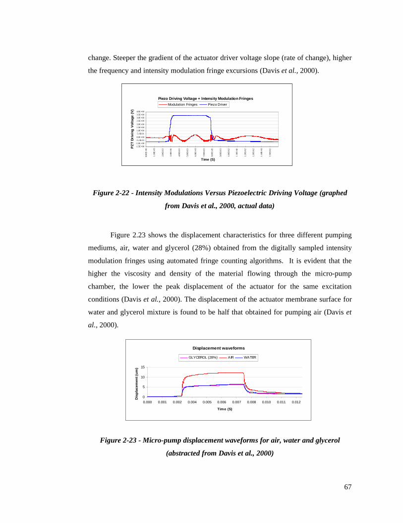
67
change. Steeper the gradient of the actuator driver voltage slope (rate of change), higher
the frequency and intensity modulation fringe excursions (Davis et al., 2000).
Figure 2-22 - Intensity Modulations Versus Piezoelectric Driving Voltage (graphed
from Davis et al., 2000, actual data)
Figure 2.23 shows the displacement characteristics for three different pumping
mediums, air, water and glycerol (28%) obtained from the digitally sampled intensity
modulation fringes using automated fringe counting algorithms. It is evident that the
higher the viscosity and density of the material flowing through the micro-pump
chamber, the lower the peak displacement of the actuator for the same excitation
conditions (Davis et al., 2000). The displacement of the actuator membrane surface for
water and glycerol mixture is found to be half that obtained for pumping air (Davis et
al., 2000).
Figure 2-23 - Micro-pump displacement waveforms for air, water and glycerol
(abstracted from Davis et al., 2000)
Displacement waveforms
0
5
10
15
0.000 0.001 0.002 0.004 0.005 0.006 0.007 0.008 0.010 0.011 0.012
Time (S)
Dis
plac
emen
t (um
)
GLYCEROL (28%) AIR WATER
Piezo Driving Voltage + Intensity Modulation Fringes
-1.5E+00-1.0E+00-5.0E-010.0E+005.0E-011.0E+001.5E+002.0E+002.5E+003.0E+003.5E+004.0E+00
0.00E
+00
1.00
E-03
2.00E
-03
3.00
E-03
4.00E
-03
5.00E
-03
6.00
E-03
7.00E
-03
8.00E
-03
9.00E
-03
1.00E
-02
1.10
E-02
1.20E
-02
1.30E
-02
1.40
E-02
1.50E
-02
Time (S)
PZT
Driv
ing
Volta
ge (V
)
Modulation Fringes Piezo Driver

68
The shape in Figure 2.24 illustrates the effect of free vibrational ringing, which
may be attributed to the rapid excursions of the membrane due to decreased resistance
whilst pumping air. This increased flow resistance for water, compared to air, was one
possible reason for the reduction in the amplitude of the actuator membrane
displacement (Davis et al., 2000) (Figure 2.23). It was also observed that when pumping
water, with identical pump cycles and piezoelectric actuator driving voltage over the
acquired sampled periods, the variability of the displacement was greater than the ones
exhibited when pumping air (Davis et al., 2000). The displacement variability observed
when pumping water could be associated with flow rate instability caused by membrane
valves (Davis et al., 2000).
Figure 2-24 - Ringing Section of Micro-pump Displacement (abstracted from Davis et
al., 2000)
The pumping medium viscosity and density determines the volume of material
that will flow through the pump chamber during each pump cycle (Figure 2.25). This is
expected during open-loop operation because piezoelectric actuators exhibit hysteresis
and creep behaviour (like other open-loop systems) and, when loaded, their dynamic
characteristics may be altered. One way of maintaining long-term position stability,
repeatability and accuracy is to include feedback control for the piezoelectric actuator.
It was shown that the pulse repetition frequency driving the piezoelectric
actuator had the effect of linearly varying the amplitude of the membrane displacement
(Davis et al., 2000). A number of pumping frequencies were plotted against the
membrane displacement, which showed a decrease in amplitude with increase in
frequency (Davis et al., 2000).
Ringing micropump displacement
02468
1012
2.50 2.59 2.68 2.77 2.86 2.95 3.04 3.13 3.22
Time (mS)
Disp
lacem
ent (
um)
WATER AIR GLYCEROL (28%)
AIR WATER
GLYCEROL (28%)

69
Figure 2-25 - Displacement During Pumping of Water (abstracted from Davis et al.,
2000)
The sampled micro-pump cycle intensity modulation fringes were analysed
using a discrete form of an adaptive filter (Figure 2.26). The maximum and minimum
points were identified and the frequency extrapolated, then converted into voltage
amplitudes by differentiating between the valid maximum points. When the frequency
is high the displacement slope is the steepest, which occurs during the rapid up and
down slope phases of the piezoelectric actuator (Davis et al., 2000). In addition to the
photovoltaic transitions, electrical and mechanical noises were added, which could be
filtered out using linear interpolation. If the excursions between the maximum and
minimum points were outside the specified amplitudes they were discarded.
Figure 2-26 - Impulse Modulation Fringe Displacement Interpolation Process (Davis
et al., 2000)
Pump Membrane Displacement while pumping water
(PUMP B)
0
1
2
3
4
5
6
7
0 0.01 0.02 0.03 0.04 0.05 0.06
Time(s)D
ispl
acem
ent (
µm)
Series1 Series2 Series3
0
50
100
150
200
250
300
1.01 1.03 1.05 1.07 1.09 1.11
Time (ms)
Pulse
Am
plitu
de (V
)
-0.4-0.3-0.2-0.10.00.10.20.30.40.5
Frin
ge A
mpl
itude
(V)
Actuator Pulse Modulation Fringes
Maximum Minimum

70
2.10 Integrated Optical Directional Couplers in Silicon-on-Insulator
In the context of this Doctoral research, it is intended that the outcomes (i.e.,
closed-loop control based on interferometric feedback) could ultimately be converted
into a viable end-product through the integration of optics, micro-mechanics and
microelectronics, and that these would be implemented on a single silicon substrate.
Trinh et al., (1995) observed that Silicon-on-insulator (SOI) technology offered great
potential for integration of optoelectronic functions on a silicon substrate.
Trinh et al., (1995) also found that SOI technology demonstrated promise for
improving the performance of CMOS electronic circuits. “This approach could also
greatly benefit the integration of micro-system components, such as micro-pumps and
electronic control using the similar materials. All of the electronic control devices,
fabricated on CMOS integrated circuit (IC), could be significantly enhanced in term of
speed and signal processing, when integrated with SOI technology. The SOI
technology had already been demonstrated in single mode wave-guides with low
propagation losses demonstrated in SiO/Si/SiO2 structures (Soref et al., 1986)”.
The application of directional couplers in the interferometer was a necessary
requirement so it followed that integration would help in the reduction of the
interferometer size. Trinh et al., (1995) found that: “SOI of great interest, as it
demonstrated that this could be achieved without losses in performance or functionality.
Directional couplers operate at 1.55µm and have an excess insertion loss of ~1.9µm.
Using SOI devices, a variety of components for wavelength-division-multiplexed
(WDM) networks could be realised in silicon IC-compatible technology”.
Trinh et al., (1995) observed that: “The bond and etch-back silicon-on-insulator
(BESOI) wafer had a SiO2 thickness of 1µm and a Si thickness of 5µm. Waveguides
were formed using a two-step reactive ion etching (RIE) process. The first SF6 etch was
performed at 100mTorr with 250W power for 6min. This was followed by a SF6/O2:
85mTorr/15mTorr etch at 250W power for 2min. The two-step etch was developed to
avoid problems associated with polymerisation of the photo resist”.

71
Trinh et al., (1995) found that: “The rib wave-guide height was 2µm and the
width is 3µm and the separation between the wave-guides in the coupling region is
2.5µm (Figure 2.27). Devices with coupling section lengths ranging from 150 to 400µm
were fabricated. Smooth S-bend sections were utilised to form input and output wave-
guides with 250µm spacing order to facilitate coupling using optical fires as shown in
Figure 2.27(a)”.
Figure 2-27 - Schematic Diagram of Symmetric Directional Coupler (abstracted from
Trinh et al., 1995)
Soref et al., (1986) observed that despite the large difference in the refractive
index between the silicon and SiO2, single mode propagation in wave-guides with large
dimension (comparable to the mode of the single mode fibre) can be obtained. Trinh et
al., (1995) determined that: “Single mode is satisfied when a/b ≤ 0.3 + r/√[1-r2]. Figure
2.27(b) shows the contour plot of the eigenmode of the rib wave-guide. The beam
propagation method (BPM) calculations show that the high-order modes, excited by off-
axis illumination, decay within distances of a few hundred microns and stable single
mode operation is observed. The propagation loss through the straight SOI ribs was
measured, using the conventional cutback technique, to be o.2/dB/cm at λ = 1.3µm “.
Figure 2.28 shows the power-split ratio against the coupling length. Trinh et al.,
(1995) provided comparison with BPM simulations of the entire structures, including
(a) Directional coupler Schematic
diagram
(b) Rib-wave-guide configuration and
numerically calculated field distribution
Coupling length
L
2aλ
2brλ
2bλ
SiO2

72
the input S-bend, the coupling section and output S-bend sections. “The best fit between
the measured data and BPM simulation is obtained for the coupler separation 2.25µm”.
Figure 2-28 - Power Split Ratio against Coupling Length (abstracted from Trinh et al.,
1995)
Trinh et al., (1995) fabricated integrated optical directional couplers on SOI
wafers using rib wave-guide. Trinh et al., (1995) demonstrated that a 3dB coupler on
SOI wafer could be successfully fabricated with excess insertion losses as low as 1.9dB.
This device was useful as key building block for Mach-Zehnder type wavelength
multiplexers/de-multiplexers. It showed the potential of SOI technology for low-cost
monolithic optoelectronic circuits.
Murphy et al., (1997) stated that: “Directional couplers required processing of
optical signals through to the photo detectors, as modulation switches had to provide the
desired power splitting ratio, independent of wavelength or polarization (Erdoga et al.,
1997, Bilodeau et al., 1997). By using conventional directional couplers, it was often
impossible to achieve broadband polarisation-insensitive performance, especially in
planar integrated devices. It was recognised, however, that wavelength-insensitive
directional couplers could be realised by cascading two conventional couplers in a
Mach-Zehender configuration (Jinguji et al., 1990, Gonthier et al., 1991)”.
The structure of the insensitive coupler is depicted schematically in Figure 2.29.

73
Figure 2-29 - Cascaded Directional Couplers (abstracted from Murphy et al., 1997)
Murphy et al., (1997) devised a device consisting of two conventional
directional couplers, cascaded in a Mach-Zehnder configuration, with a relative phase
shift introduced between them. “The device achieves insensitive performance through a
fractional change in wavelength (or polarization, refractive index, waveguide size, etc.),
which tends to affect each directional coupler in the same way. The relative phase shift
between the two couplers causes these deviations to balance each other such that the
resulting power splitting ratio remains unchanged (Equations 19, 20 and 21). The
splitting ratio at the output of the device can be expressed in terms of three
dimensionless quantities, Ф1, Ф2, and 2θ (Jinguji et al., 1990, Little et al., 1997):
Equation 19 S = cos2 θ sin2(Ф 1 + Ф 2) + sin2 θ sin2(Ф 1 _ Ф 2)
Ф 1 and Ф 2 represent, respectively, the total integrated coupling of the two
constituent directional couplers, and 2θ is the relative phase shift, which separates them.
Each of these parameters depends implicitly upon wavelength, polarization, etc. As
described in a previous work by Little et al., (1997) insensitive performance is achieved
by choosing these three parameters in the following way:
Equation 20
−=
+=
NN11
83,11
83
21
ππ φφ
Equation 21 1
2
23sin
23sincos
−
+
=
NN
Nππ
θ

74
where N is a dimensionless real parameter larger than 3. N can be chosen to give any
desired splitting ratio as described by Trinh et al., 1995. In the case where 50% splitting
is required, N = 3 and the solutions are particularly simple”:
Equation 22 Ф1 = π/2, Ф2 = π/4, and θ = π/3.
Murphy et al., (1997) calculated that: “Knowing the three quantities Ф1, Ф2, and
2θ, a waveguide device was designed to nominally achieve the desired accumulated
coupling factors, and phase shift by selecting a suitable waveguide geometry and
material system. Based upon vendor-supplied information about the refractive indices at
λ = 1:55 μm, a waveguide geometry was designed to yield efficient coupling to an
optical fibre. Using coupled mode theory, the waveguide was calculated whilst coupling
as a function of separation, and with this information two directional couplers were
designed (Figure 2.30). The phase shift 2θ was achieved by making one arm of the
interferometer slightly longer than the other. For all calculations, a free-space
wavelength of 1.55 μm was used. Figure 2.29 illustrates the important design
parameters”.
Figure 2-30 - Cross Sectional Diagram Illustrating Waveguide Geometry at Point of
Closest Separation (abstracted from Murphy et al., 1997)

75
Murphy et al., (1997) ensured that: “The patterns were carefully placed to insure
that each device does not cross an e-beam field boundary, which could introduce
spurious phase shifts. For comparison, the design included a set of conventional
directional couplers, designed to achieve 50% splitting ratios at λ = 1:55 μm and with
waveguide geometry at point of closest separation”.
Murphy et al., (1997) shows in Figure 2.31, plots of the splitting ratio vs.
wavelength for a conventional directional coupler that yield an improved insensitive
coupler. “Note that the conventional coupler achieves a splitting ratio, which is
uniformly higher than the nominal value of 50%. This discrepancy was attributed to (i)
uncertainty in the material indices of refraction used in the calculations, and (ii)
structural and material deviations from the nominal design which may occur during the
various fabrication steps. In principle, this bias can be removed by performing a more
exhaustive empirical investigation of the material properties and by carefully controlling
and characterizing each step of the fabrication process. However, in addition to this
offset, the conventional coupler exhibited a sloped wavelength dependence, which was
characteristic of directional couplers and could not be flattened without using a
completely different design”.
Figure 2-31 - Measured Power Splitting Ratio vs. Wave-length for Two Cascaded
Devices (abstracted from Murphy et al., 1997)
76
Murphy et al., (1997) shows that: “The upper two curves in Figure 2.31
represent the measured splitting ratio for a conventional coupler (TE and TM
polarizations), and the lower two curves correspond to the parameter-insensitive Mach-
Zehender coupler”.
Murphy et al., (1997) concluded that: “By more carefully controlling and
characterizing the materials and fabrication, it was possible to bring these devices closer
to the nominal design, which should further improve their performance”.

77
2.11 Integrated Optical Sensor Considerations
Erickson and Li (2003) stated that: “The integration of high-resolution optical
sensing elements that make up a fibre optic interferometer into micro-fluidic devices
such as a micro-pump, is necessary for constructing a portable lab on-chip device.
Adams et al., (2003) developed a technique that was used to integrate replica moulded
micro channel systems with a complementary metal oxide semi-conductor (CMOS)
imaging chip to develop an on-chip adsorption or fluorescence micro spectrometer”.
Erickson and Li (2003) observed that: “It became possible to obtain absorption
signatures for dilute dye solutions. Camou et al., (2003) introduced a lens with
embedded input and output optical fibres and 2D lenses for integrated fluorescence
spectroscopy. The integration of lenses was shown to increase the sensitivity of the on-
chip detection method three-fold over the lens-less device. In their work, Ruano et al.,
(2003) described the micro-fabrication processes required for the successful
manufacture, integration and packaging of a micro-array of integrated optical sensing
elements. Both optics and fluidics were integrated into the device. A pumping system
for delivering small amounts of fluid across the array was also described. Baechi et al.,
(2002) presented a highly integrated micro-channel system with integrated valves (up to
330 valves/cm2), heaters and photodiodes that was used for parallel processing and
detection of nano particles. The valves on this device were actuated by a unique
themopneumatic technique that involves the heating of a confined air cavity. An
interesting discussion of thermal cross talk on such a device and a cooling method are
provided by Haefliger et al., (2000)”.
The integration of the optical sensor such as the interferometer described in this
research would greatly increase the resolution of the detection whilst at the same time
decrease environmental interferences. Mohammed et al., (2004) states that: “This type
of integration has already been attempted with the development of a high-speed, 6-
channel parallel optical transceiver package used to demonstrate the viability of chip-to-
chip optical I/O in Very Large Scale Integration (VLSI) circuits. The package concept

78
was developed to be compatible with the microprocessor package technology and, at the
same time, allow the integration of low-cost, high-performance optical components. Pin
photo detectors, polymer waveguide arrays with Multi-Terminal (MT) connectors as
well as CMOS transceiver chips were heterogeneously integrated on a standard
microprocessor Flip-Chip Pin Grid Array (FCPGA) substrate. The main advantages of
this approach included compatibility with the IC packaging industry, parallel
transmission architecture that increases throughput, an MT optical port that alleviates
distance limitations between two packages (multiple applications), passive alignment,
and contains self-testing capability circuit”.
Mohammed et al., (2004) shows (Figure 2.32) the optical assembly on the
FCPGA substrate that has a transmitter and a receiver portion that are symmetrically
situated with respect to the CMOS transceiver chip at the centre of the substrate.
Figure 2-32 – FCPGA plus optical assembly integration
Mohammed et al., (2004) developed: “The waveguide array has a core
dimension of 35x35 µm2 and was fabricated from acrylate, using photo bleach
processing”. Mohammed et al., (2004) used polymer waveguides due to their potential
FCPG
A
GaAs photodiode
Pin Laser diodes
Polymer Waveguide
Receiver Trans-conductance buffer, CMOS
Microprocessor Flip-Chip Pin Grid Array (FCPGA) substrate
Transmitter Driver buffer

79
for high-volume, low-cost production. The acrylate-based multimode polymer
waveguides are known for their low loss (0.08 dB/cm), ease of integration, best system
performance, and manufacturability. The detailed processing can be found in
(Schmidtchen et al., 1991). The transmitter includes an optical source array and a
polymer waveguide arrays that are flip-chip bonded on the substrate and coupled to
polymer waveguides with 45-degree metal mirrors to direct light at right angles for
transmission through the waveguide. Similarly, the receiver consists of identical optical
waveguide assembly to the transmitter section, with a high-speed GaAs photodiode at
the input array”.

80
2.12 Summary of Literature Review
A number of significant areas were identified during the course of the literature
review and these contributed towards the research directions and methodology adopted
in this Doctoral research program. The technological advancements in the area of
MEMS, microelectronics and optics, significantly increased the research momentum.
Many of these papers related to building and modelling of micro-pumps that were
characterised using open-loop responses. Some, on the other hand, discussed
techniques that took into account external sensors, such as heaters, polarised channels,
thermo-resistors, thermo-couples, radiation sensors, charge coupled devices,
pyroelectric, magnetic, chemical and pressure sensors. These sensors were generally
added externally to monitor the:
• Flow rate
• Volume
• Temperature
• Velocity
of the medium being transferred through the micro-pump chambers. However, these
did not directly lead to control of the micro-pump parameters based on the feedback
elicited by the sensors.
It also became evident that a free-vibrating micro-pump PZT actuator exhibited
substantial variations whilst pumping gases and liquids of varying densities, which
could be attributed to impurities in the media and irregularities in the excitation of the
PZT material, in this case a diaphragm attached to the PZT membrane.
It was well established that the frequency and the amplitude of excitation
directed at the PZT membrane could be used to precisely control the volume and flow-
rate of the fluid transferred through the micro-pump chambers, as long as frequency and
amplitude are varied in real-time, with a minimum amount of latency between analysis

81
and control. The literature review revealed the need for a non-contact sensing method
to be developed, which could be applied within the confines of the very structure being
monitored and without impeding its operation and performance.
Considering the design and structure of a micro-pump, an effective way of
monitoring displacement is through the use of a non-contact fibre optic interferometer.
This approach would leave an air gap between the actuator membrane surface and the
laser light delivered through the focusing lens and fibre tubing. Other approaches such
as the optical lever or non-contact pressure sensor (capacitive) technique could also be
applied, but the complexity of multi channelling, and the irregularity of the capacitive
response would greatly reduce the accuracy of the measurement.
By undertaking research into the most suitable non-contact sensors for
measuring the displacement of a micro-pump’s PZT actuator, and characterising its
performance, it was potentially possible to identify parameters that, when varied, could
influence the characteristics of the response. With the ability to destabilise the
equilibrium of the response by simply varying any number of controlling elements, and
by carefully characterising the open-loop response, it was possible to close the loop and
then implement an adaptive feedback, which would allow for self monitoring and
calibrating.
Ideally, a practical closed-loop micro-pump needed to be fully integrated with
optics and microelectronics in a single structure. Some of the major components
identified as relevant to the central research theme were:
• Optics, Sensing (photodiodes), driving (laser diodes), passive optics (fibre,
directional couplers, mirrors, lens)
• Micro-pump structures
• Piezoelectric membrane
• Microelectronics
• Electronic components

82
• Amplifiers, Analog-to-digital converters (ADCs), memory, microprocessor
and a complex programmable logic device (CPLD).
The literature review revealed a significant number of research papers associated
with open response analysis of micro-pumps driven by piezoelectric actuation, but many
of these concentrated on the construction and materials that were employed, rather than
the performance analysis based on the actuator deflection. A number of models were
based on electrical equivalent circuits, and these were represented using mathematical
models. This was useful in generating characteristic behavioural patterns for the PZT
materials that were used to contort the metal diaphragm during the application of a high
voltage pulse. The deflection pattern aided in finding the optimum point, at the actuator
membrane surface where the strongest deflections of the laser beam occurs.
The literature review also revealed the optimum voltage potentials for the
piezoelectric material at which the maximum strength is attained (200 V to 400 V dc.).
In many cases, depending on the pressures associated with the micro-pump chambers,
the driving voltage was as low as 50 V dc. The only drawback was the flow rate and the
pumping medium limitations that were associated with such a low voltage system and,
hence, a 400 V micro-pump was chosen for this research.
A number of fibre optic interferometer configurations were reviewed, but none
were as accommodating as the Mach-Zehnder type. The primary concern about this
related to its physical size, and the practical implications when interfacing with a micro-
pump that was approximately 12 mm in diameter.
In the context of closed-loop control of micro-pumps, the literature review did not
reveal any papers which reported research that directly associated the actuator
displacement with the flow rate. Specifically, no published work was uncovered
describing micro-pump control through the application of fibre optic interferometer
feedback.

83
3 Design and Construction of Open and Closed-
loop Test Platforms

84
3.1 Overview
3.1.1 Design Sequence and Rationale
In order to characterise the open-loop and closed-loop response of a micro-pump
using a fibre optic interferometer, a number of electronic modules were constructed to
meet the detection and sensing requirements for processing of the interferometer optic
information. The modular design was developed in two stages, the first of which
incorporated two discrete elements, comprising a photodiode amplifier and a dynamic
digital processing module. The second stage integrated an analog, digital and
piezoelectric driver, allowing for more uniformity and flexibility when considering
closed-loop operation. The fibre optic interferometer was constructed from:
• A single-mode fibre
• Two directional couplers
• Collimating and focusing lens
• Neon Helium laser source.
The design of the open and closed-loop systems was based upon the following
developmental sequence and rationale:
(i) Simulation
In-circuit Spice models were implemented for the following elements
• Photodiodes
• Photodiode amplifiers, trans-conductance.
• Differential signal conditioning models
• Data acquisition modelling
• Bipolar modelling

85
(ii) FPGA timing and functional modelling
§ Data processing hardware
(a) ADC interface
(b) FIR filter
(c) Memory segmentation
§ error coefficients
§ % variation
§ average error displacement
§ PZT compensation coefficients
§ displacement data
§ serial communication buffer
§ compression processing RAM
(d) Serial communications interface
(e) Piezoelectric Driver
§ Pulse shaping generator modelling
§ Pulse driver circuit simulation
§ High Voltage (HV) amplitude shifter
(iii) CPU emulation
§ Serial peripheral Interface (SPI) bus for data transfer protocol
implementation
§ Analog-to-digital (ADC) serial processing for opto-sampling
verification during trans-conductance processing.
§ PZT driver feedback-loop monitoring (ADC channel) for
calibration verification.
This chapter describes the design of the electronics and interferometer that were
developed in order to provide a laboratory-based characterization of the micro-pump.
The details provided herein, concerning the design and development of the discrete
component test system will give some insight into the significant challenges, and
complexity involved, in creating a system that could provide an accurate micro-pump
characterization. The development of the electronic testing system was undertaken with

86
a view to subsequent closed-loop micro-pump operation, and in consideration of the
fact that any practical system would ultimately have to be fabricated into a package of
comparable size to the micro-pump itself
The first step in the development and characterisation process was to determine
the efficacy of using an interferometer as a feedback device for a piezoelectric actuator.
This is described in Section 3.1.2.
3.1.2 Characterisation of a Piezoelectric Actuator Using a Low-Coherence
Interferometer
As a preliminary step in the development of a closed-loop system, it was
necessary to determine the viability of the interferometer as a feedback device. An
experimental set-up was configured on a laboratory bench, using air as the transference
medium. This is shown in Figure 3.1.
Figure 3-1 - Michelson Interferometer
Data acquisition
and processing
PZT Driver
Laser Light Source
(LS)
Reference mirror (RM)
Range of reference mirror
displacement
Photodetector (PD)
Photodetector
Piezoelectric actuator (PA)
Beam splitter (BS) a Lens Approx. 45°
Av PC
Amplifier
Diverging Lens (DL)

87
This type of interferometer was used to study the displacement measurement of a
piezoelectric membrane, including piezo-ceramic transducers, such as sound tweeters
and beepers. It was convenient to apply the interferometric theory on a tangible system
and then apply it to a more complex fibre-optic configuration. A Michelson
interferometer was built and used to measure the fringe modulations and determine a
behavioural model of a system for measuring the displacement of a varying frequency
piezoelectric transducers and materials of the types used in development of micro-
pumps. The first experiment (Figure 3.1) was carried out in air with a continuous wave
method for materials characterisation and performance quantification using sources of
different coherence lengths in a scanning Michelson interferometer. The data was not
tabulated and the information relating to the generation of the interferometric fringes
was useful in transposing the technique into the experimental model described by this
research (Section 3.3, Figure 3.4).
The basic theory of operation is relatively straightforward. A laser beam travels
to a beam-splitter, through a diverging lens, where it is split into two beams. One beam
is transmitted through the beam-splitter to the piezo-actuator (PA) surface and the other
beam is reflected at 90 degrees to the reference mirror (RM). The distance or path
length between each mirror and the beam-splitter (BS) should be the same (< 25mm).
These distances were determined with a tape measure, and were made as long as
possible for the test platform size, because the interferometer's sensitivity increased with
the separation distance between the mirrors and the beam-splitter.
Both the reference mirror and the piezo-actuator surface reflected their respective
beams back to the beam-splitter and struck the beam-splitter at the original incident
beam's position. Part of the piezo-actuator’s reflected beam was then reflected by the
beam-splitter to the photo-detector (PD), and part of the reflection mirror’s reflected
beam was transmitted by the beam-splitter to the photodiode surface. Two beam spots
were visible on the photodiode surface. The objective was to superimpose the two
reflections produced by the beams until they were perfectly aligned when the piezo-
actuator membrane was static. The spots could be approximately superimposed by

88
moving the reflection mirror left, right, up or down. Additional precision could be
achieved if a diverging lens (DL) was placed between the laser and the beam-splitter.
By placing the diverging lens close to the beam-splitter, the diameter of the two beam
spots on the photodiode surface increase, making them easier to superimpose.
This initial experiment demonstrated that, fundamentally, interferometric fringes
could be used to measure displacement of undulating surfaces, but also that resolution
was limited due to ambient interference if an air medium was used. When undulations
in the micrometre range were considered, a more stable and reliable system had to be
investigated and this was achieved through the use of fibre-optic channelling.
Although interferometry was a useful and accurate technique for measuring
displacement, it was not the only high-resolution optical method that could be used to
measure such small strains. Another method that was also considered in the initial
stages of research was the use of optical levers that could be used to measure small
changes in displacement. An optical lever is a non-interferometric device, where the
power of a light beam striking a vibrating surface is modulated in such a way that the
power of the reflected beam is proportional to the displacement of the surface (Figure
3.2).
Figure 3-2 - Optical Lever displacement sensing technique
To Photocell Laser Source
Phase-to-Target
Displacement
Light Transmitting Fibre
Optic Filament
Light Receiving Fibre
Optic Filament
PZT Sample

89
This technique was considered of potential value to this Doctoral research
because it could be used for validation of the interferometric data.

90
3.2 The Micro-pump
3.2.1 General
The characterization process was undertaken on an “IMM” self-priming
membrane micro-pump (Figure 3.3) capable of flow rates up to 750 µl/min, and
powered with a 400 Vpp, generated from a low 5V dc source, and a 5 ms pulse.
Figure 3-3 - Self Priming Membrane Micro-pump
The micro-pump cover was removed, exposing the actuator surface for the
purpose of non-contact interferometric testing. The surface of the actuator diaphragm is
generally not very reflective and rather rough, which did not present well for interfacing
with the interferometer projection, and finding an optimum reflective point was
difficult. Initially, a thin layer of a reflective material was considered for adhesion to
the actuator PZT membrane, but it was found that the interference with the micro-pump
performance would be too great. The other issue was with the adhesion of the material
to the PZT membrane, where it had to maintain its surface characteristics during the
flexing of the PZT material. After some basic experimentation, however, it was
determined that the surface of the PZT membrane, irrespective of its surface properties,
Pump chamber
Outlet valve
Piezoelectric actuator
Diaphragm
Solid substrate layers
PZT electrode (+)
PZT electrode (-)
Outlet Inlet
Valve membrane
Inlet Valve

91
produced a sufficient amount of cohesiveness between the interferometer and the
photodiode detectors, which could be interpreted and processed by the central
processing analysis module. It was found that the reflection from the fibre tip and that
from the actuator membrane surface produced optical modulation fringes with the
advantage that the target need not be critically aligned, since the reflected light was
dependant on the target angle and distance from the optimum focus. This resulted in a
typical range of 2mm and a maximum angular target error of 1 degree.
3.2.2 Micro-pump Operation
Applying a pulse to the micro-pump actuator membrane causes it to deflect
upwards, which in turn creates a decrease in the main chamber pressure and increases
its volume potential that forces the liquid or gas pumping medium to fill the vacuum.
During the downward deflection of the actuator membrane, caused by the removal of
the pulse, the pressure in the main chamber increases while the volume decreases,
forcing the liquid or gas from the main chamber and exit through the outlet valve.
Piezoelectric actuation, as shown in Figure 3.3, has the advantage of being able to
produce a reasonably high stroke volume; a high actuation force and a fast mechanical
response that makes it a very attractive, and frequently used, actuation principle for
micro-pumps. One disadvantage is the requirement for a comparatively high actuation
voltage (400 Vpp) Another disadvantage is the mounting procedure for the PZT disk
that requires a very specialised gluing process. However, published research indicated
that the process optimisation of the mounting procedure could significantly improve
reliability and yield for this type of actuator (Kluge et al. 2001, Richter et al. 2001).
Alternatively, different processes, such as screen printing (Koch et al. 1997, Koch et al.
1998), and thin-film depositing of PZT material had also been investigated. These
techniques also proved to be feasible, but the resulting strokes (typically 1 µm at 100 V
(Koch et al. 1997)) were small in comparison to glued PZT bulk material (e.g., 15 µm at
100 V (Koch et al. 1997)). To achieve higher strokes for lower actuator voltages,
optimisation of the geometrical design was reported by several researchers (Linnemann
et al. 1998, Morris et al. 2000). Once optimised, the typical actuation voltages were in

92
the range of 100 V (e.g., 130 VPP for the micro-pump (Woias et al. 1998)), which was a
significant improvement in comparison to other micro-pumps that employed
commercial piezo buzzers without any optimisation (e.g., 400 VPP) (Kämper et al.
1996)). This lower actuation voltage was also helpful for the design of highly
miniaturised electronic drivers, which allowed for low-power operation from a battery
(Woias et al. 1998).

93
3.3 The Fibre Optic Interferometer Construction
The dynamic displacement of the micro-pump actuator membrane was measured
using a fibre-optic interferometer (Figure 3.4) in a Mach-Zehnder configuration, using a
communication grade 600 nm to 1550 nm single mode fibre (SM), driven by a Helium
Neon (HeNe) Melles Griot 1.2 mW laser source, with a wavelength of 632.8 nm . This
was split with two fibre-optic directional couplers and input to an amplifier for
progressive processing and analysis.
Figure 3-4 - Open-loop Fibre Optic Interferometer
The experimental interferometer was fabricated from standard discrete
components that would eventually need to undergo miniaturization and integration
based on the polymer or silicate substrates. The interferometer signal beam was focused
at the micro-pump actuator membrane maximum displacement position, typically at the
centre. The focusing apparatus determined the distance from the optimal displacement
position, such that the maximum signal intensity and integrity was achieved. The laser
beam signal PL was directed through a 3dB fused fibre optic directional coupler and
PZT stretcher
DC 2
DC
1
Focusing lens
Collimating lens
632.8 nm HeNe 1.2 mW Laser
signal
ref
P L
P S
P M
P R
Directional couplers
To/Fr om micro-pump actuator membrane
surface
To Optical detectors
From compensation
Driver
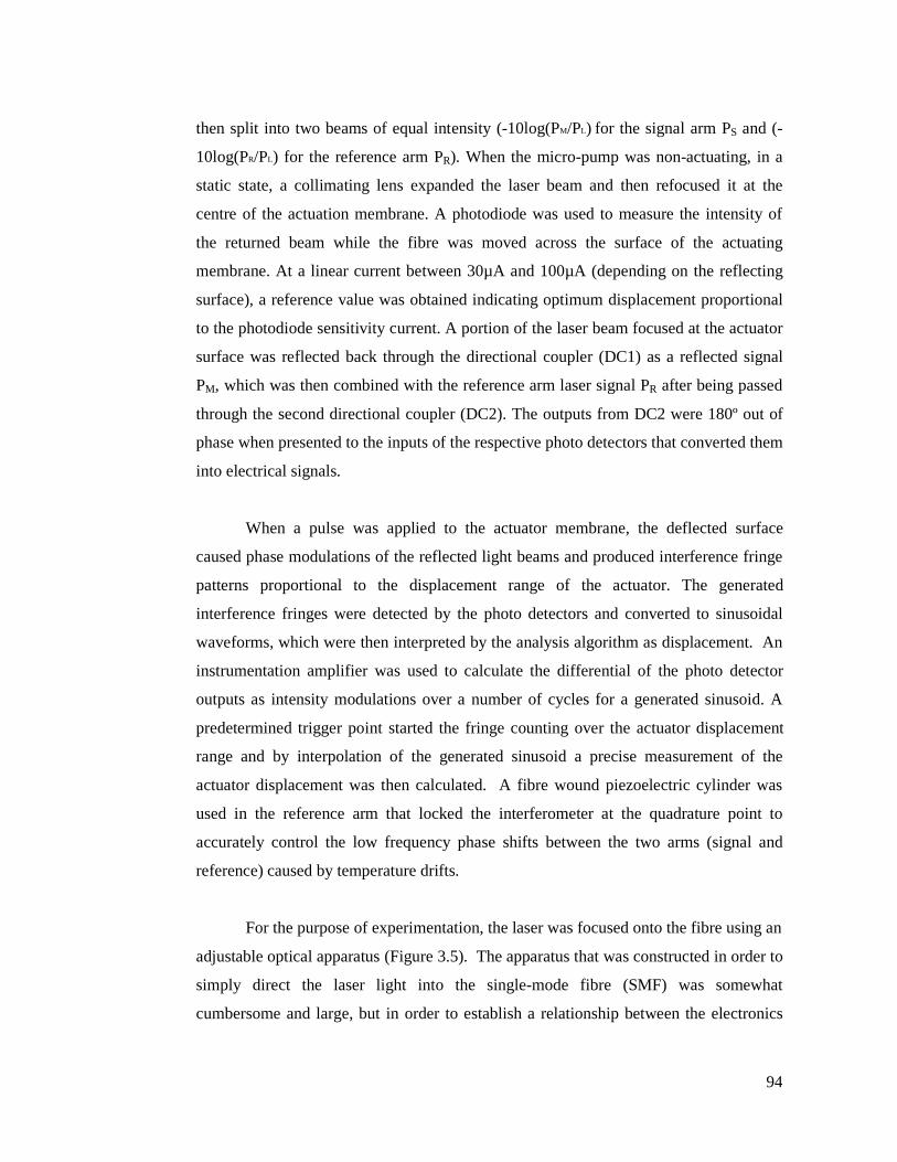
94
then split into two beams of equal intensity (-10log(PM/PL) for the signal arm PS and (-
10log(PR/PL) for the reference arm PR). When the micro-pump was non-actuating, in a
static state, a collimating lens expanded the laser beam and then refocused it at the
centre of the actuation membrane. A photodiode was used to measure the intensity of
the returned beam while the fibre was moved across the surface of the actuating
membrane. At a linear current between 30µA and 100µA (depending on the reflecting
surface), a reference value was obtained indicating optimum displacement proportional
to the photodiode sensitivity current. A portion of the laser beam focused at the actuator
surface was reflected back through the directional coupler (DC1) as a reflected signal
PM, which was then combined with the reference arm laser signal PR after being passed
through the second directional coupler (DC2). The outputs from DC2 were 180º out of
phase when presented to the inputs of the respective photo detectors that converted them
into electrical signals.
When a pulse was applied to the actuator membrane, the deflected surface
caused phase modulations of the reflected light beams and produced interference fringe
patterns proportional to the displacement range of the actuator. The generated
interference fringes were detected by the photo detectors and converted to sinusoidal
waveforms, which were then interpreted by the analysis algorithm as displacement. An
instrumentation amplifier was used to calculate the differential of the photo detector
outputs as intensity modulations over a number of cycles for a generated sinusoid. A
predetermined trigger point started the fringe counting over the actuator displacement
range and by interpolation of the generated sinusoid a precise measurement of the
actuator displacement was then calculated. A fibre wound piezoelectric cylinder was
used in the reference arm that locked the interferometer at the quadrature point to
accurately control the low frequency phase shifts between the two arms (signal and
reference) caused by temperature drifts.
For the purpose of experimentation, the laser was focused onto the fibre using an
adjustable optical apparatus (Figure 3.5). The apparatus that was constructed in order to
simply direct the laser light into the single-mode fibre (SMF) was somewhat
cumbersome and large, but in order to establish a relationship between the electronics

95
and the optics, a working platform of practical proportions was necessary. The initial
stages, based on the Mach-Zehnder platform, required careful investigation in order to
generate a proof-of-concept, so a practically accessible system of a reasonable size was
constructed. Figure 3.5 incorporated a 1.2 Watt Neon Helium laser, with fibre driving
optics clamped with adjustable bench apparatus, at least 30 cm long, 10 cm wide and 12
cm high. , Figure 3.6 shows a polystyrene box, 70 cm long, 38 cm wide and 38 cm high
housing the fibre optics and the directional couplers, while Figure 3.7 illustrates the
termination of fibre optics by the use of microscope optics, and associated fine
adjustment apparatus (20 cm long, 7 cm wide and 8 cm high).
Figure 3-5 - Laser and Fibre Driving Optics
Figure 3-6 - Fibre and Optical Components

96
The apparatus was clamped and secured onto a laboratory bench, allowing for
adjustments of the laser proximity to the focusing lens and as well as to the optical fibre
end. Securing the fibre within a universally adjustable clamp, it was possible to move
the fibre end in a three dimensional array by simply adjusting the x, y and z parameters
of the clamp.
To set for optimum point of laser intensity to the optical fibre end, it was only
necessary to watch the fibre strand at the output of the clamp that produced high
intensity brightness along its length. Since there were a number of dynamically variable
parameters available for adjustment, a reference beam was focused at the fibre end and
then the clamp x, y and z adjustments were altered until the optimum intensity along the
fibre shaft was achieved. It was for this reason that a visible infrared wavelength was
used (632.8µm). The only sacrifice then was in the overall frequency response
bandwidth that needed to be compensated by the use of high-cost, high-speed
operational amplifiers.
After adjusting the angle of the laser beam, and the focus for optimum light
absorption by the fibre, light was passed through the interferometric circuit (Figure 3.6),
which was encased in a shockproof polystyrene enclosure in order to eliminate
environmental interference.
The SMF was passed through a small opening on the side of the polystyrene
enclosure, where it entered the optical circuit wiring as described in Figure 3.4, and then
emerged at three different exit points. One was for the micro-pump and focusing optics,
as shown in Figure 3.7, and the other two for the reflected optical modulation fringes.
An additional input to the polystyrene enclosure was used specifically for the fibre optic
stretcher that was driven by the controlling electronics.

97
Figure 3-7 - Micro-Pump and Focusing Optics
The size of the interferometer required a level of performance from the sensing
electronics that would compensate for the inevitable temperature drifts and vibrations.
In order to deliver a clean optical signal to the micro-pump, it was also necessary to
refocus the laser beam at the point of fibre exit (Figure 3.7), which was made easier by
the use of a visible infrared laser source.
The output for the fibre that delivered the laser beam to the surface of the PZT
membrane and also absorbed the reflections of its surface was fed into the micro-pump
focusing optics. The fibre was secured using a universally adjustable clamp and then
positioned approximately 2 - 5mm from the focusing lens. The focusing lens was also
adjustable with respect to the surface of the PZT membrane, which allowed for the
adjustment of the beam based on the intensity at its surface.
The micro-pump was glued to the back plate in a vertical position with the PZT
actuator membrane towards the focusing lens. The inlet and outlet tubes were directed
towards two solution dishes (each 10mm deep and 50mm in diameter) – one dish being
the supply tank and the other a receiver tank.

98
3.4 Development of Electronic Test Platform
3.4.1 Overview
The detection electronics were composed of a photo detector, instrumentation
amplifier, and an analog to digital converter. These had to be integrated into a
functional system with suitable processing hardware and software in order to make a
workable laboratory test system for micro-pump characterization.
3.4.2 Detection Elements and Parameters
The fibre optic interferometer required feedback compensation for the low-drift
induced phase changes in order to precisely lock the interferometer at the quadrature
point (Figure 3.8).
Figure 3-8 - Interferometer Optical Detection Closed-loop Feedback Path
The compensation factor can be expressed as a function of the error where the
controlling element is a phase shifter. The phase shifting mechanism is a piezoelectric
fibre stretcher driven by a phase detector and a feedback amplifier.
+
PM
PR+φ
Detector and
Control
PI+γ +
Signal processing and analysis
±γ ±φ
PI
PD
Modulation fringes
Laser source reference
Ambient interference

99
3.4.3 Photodetectors
The photo detector was comprised of a visible to near-infrared (Vis/NIR)
germanium photodiode with a wavelength of 1550 nm, which acted as a light controlled
current source, operating in its linear range, and an amplifier where the current was
converted to voltage proportional to the amount of light. A photodiode is very linear
over a number of light intensities making it ideal for measuring absolute light levels.
However, since the open circuit forward voltage drop across the photodiode varies
logarithmically with light level and due to its large temperature coefficient, the diode
voltage is not ideal for accurately measuring light intensity.
The shunt resistance RSH can be anywhere from 100M Ohm to > 1G Ohm at
room temperature and subsequently decreases by a factor of two for every 10°C rise in
temperature. Diode capacitance CJ depends on the actual junction area and the bias
voltage applied. In this case, the diode junction capacitance was in the order of 3 to
10pF at zero bias. Table 3.1 shows the typical diode characteristics based on its
operational parameters that govern the overall in-system performance.
Manufacturer: UDT Sensors Inc.
Type: High Resposivity (VBIAS=-5V), PIN-HR040
Sensitivity: 0.37 A/W at 632.8 nm
Max. Linear Output Current: 100µA
(Photovoltaic Mode)
Area: 0.77 mm2
Capacitance:
(@5V reverse bias) 4.5 pF
Shunt Resistance: 1011 ohm
Rise-time: 1.0 ns
Dark Current:
(@5V reverse bias) 0.30 nA
Table 3.1 - Photodiode Characteristics

100
Photodiodes can be operated with zero bias, which is photovoltaic mode or
reverse bias, the photoconductive mode (Figure 3.9). This research looked at both of
these methods, where the photovoltaic mode was chosen for its precise linear
operational characteristics and low noise, which is basically the thermal noise generated
by the shunt resistance RSH, and the photoconductive mode due to the higher switching
characteristics for increased bandwidth operations, but with some additional noise
induced due to conduction (Johnson and Shot). The reverse bias for the HR040 diodes
was set at –5V dc in the photoconductive mode and to 0V (ground) in the photovoltaic
mode (Figure 3.9).
Figure 3-9 - Photodiode Modes of Operation
Under reverse bias conditions, a small amount of current (dark current) flowed
even though the diode was not illuminated, and the total circuit noise and the dark
current limited the dynamic range. The effect of the dark current could be eliminated by
various compensation techniques, which in this case is a variable capacitor at the input
of the amplifier.
3.4.4 Photodiode Amplifiers
Optimization of photodiode amplifiers presented challenging design problems,
because high bandwidth and direct coupling were required. For the purpose of this
investigation, an analog system module was developed to meet the specification
parameters of the photodiodes described in Table 3.1. Figure 3.10 shows a general
Photodiode
0V (gnd)
ISC
Photovoltaic mode
Photodiode
-5V dc
ISC
Photoconductive mode

101
block diagram identifying a number of key functions required to meet the overall
system performance when integrated with the signal-processing module.
Figure 3-10 - Photodiode Amplifier and Signal Processing Block Diagram
A differential instrumentation amplifier, operating in a bandwidth of around 350
KHz for gains less than 10, and having low noise characteristics (typically 3 nV/√Hz) at
large gains and, is required in order to efficiently extrapolate the interferometric fringe
patterns generated during micro-pump actuator displacement measurement.
Figure 3.11 shows the photo detector amplifier module designed and used
during the experiments conducted in this research. Initially, the module was used
without the signal processing interface module, where the output signal analysis was
performed using an oscilloscope and a National Instruments data acquisition card
located in a PC. The in-system signal analysis is performed when the module is
connected to the processing unit of Figure 3.21.
Programmable Logic Device (Signal Processing)
Opt ical Signal Detector Amplifier (Analog detection)
Photodiode Amplifiphoter
[signal]
Photodiode Amplifier
[ref]
Differential Input
Amplifier [>100V CMRR]
Variable Gain Amplifier
DC Offset Adjustment
Gain Adjustment
CMRR Balance
Fast Integrator
Reset
Unity Gain Buffer
PZT Fiber Stretcher
Photodiode Sign al
Photodiode Reference
∆ ∑ ADC +
50 Hz Filter >110dB rejection
Serial to Parallel
Converter FIR
Filter
Phase & Peak Detector
Differentiator
Intensity
Modulation Interpolation
Algorithm
FIFO
Direction Finder
Coeffic ients RAM/ROM
DPRAM
SPI
Interface
Parallel to Serial
Converter
∆ ∑ DAC
PC Oscilloscope

102
The photo detector amplifier section was made up of a number of amplifier
stages, each biased for optimum performance, based on the characteristics of individual
operational amplifiers used.
Figure 3-11 - Photodiode Amplifier Module and Signal Processing
In order to minimise the effect of input bias currents and allow for detection of low
photocurrents, wideband JFET operational amplifiers were selected. Additionally, in
order to achieve linearity up to 350 KHz frequency bandwidth, the JFET-input
operational amplifier had to have high unity gain-bandwidth product, and a low input
capacitance. The bandwidth for the preamplifier fbw is given by:
Equation 23 ,2 xf
bw CRfuf
π= (where Cx = Cj + Cin)
Figure 3.12 represents a trans-conductance amplifier, showing the elements that
dynamically affect the overall response related to frequency and bandwidth. Based on
the test platform input photo detector junction capacitance (Cj ) of 4.5 pF, and the
amplifier input capacitance (Cin) of 1.8 pF, gain feedback resistance (Rf) of 39 K ohm,

103
and the unity gain-product (fu) of 16 MHz, the operational amplifier unity-gain
frequency bandwidth (fbw) is 3.22 MHz. The reactance Xcf stabilised the oscillations of
the first stage, but reduced the bandwidth, which was an issue because the photodiode
wavelength was 632.8 nm. If the actuator was driven with a high slew-rate square wave,
the frequency of the fringes could exceed the non-unity gain (>4) bandwidth (350 KHz)
for the trans-conductance amplifier (TCA) and the slope of the actuating pulse
controlled the -3 dB bandwidth cut-off.
Figure 3-12 - Fringe sensing and conversion
Ambient interference (Figure 3.8) at the input to the photo-detector may be
sufficiently high to induce fringe pattern distortions, which had to be minimised or
eliminated all together. Most were eliminated by simply switching off the fluorescent
lights, acoustic noise (microphone effect at the input to the amplifier) and vibrations.
3.4.5 Instrumentation Amplifier
A differential instrumentation amplifier is required to operate in a bandwidth of
around 350 KHz with low noise characteristics (< 3nV/√Hz) in order to efficiently
extrapolate the interferometric fringe patterns generated during the actuator
displacement measurement (Figure 3.13). For stabilization, a feedback capacitor Cf
was included as the phase shift at the frequency of intersection fbw, would cause
instability and oscillation. Introducing a zero at fbw, by adding the feedback capacitor Cf,
TCA
I D
V o = I D ? X cf ||R f
R f
X cf
Photodiod Photo Current
I SC R SH C J
0V
C in

104
stabilised the circuit and produced a phase margin of approximately 45 degrees. For the
purposes of experimentation here, the bandwidth had to be ≤ 350 KHz, which was
dependant on the slope of the actuator pulse and the amplifier characteristics. If the
PZT membrane displacement was driven with a high slew rate square wave, the
frequency of the fringes could be as high 600 KHz when pumping air.
Figure 3-13 - Fringe Sensing and Processing
Figure 3.14 shows the Bode Plot for the photodiode amplifier response based on
the gain of 26. Note the bandwidth at -3dB is 351 KHz.
Figure 3-14 - Fringe Sensing and Processing
TCA AV
DAV1
TCA AV
V o
I SD
I RD
A sg1 = I SD • X c||R f
A rg1 = I RD • X c ||R f
A sg2 = 10
A rg2 = 10
A srg1 = 2 A srg2 = 10
DAV2
R f
X c
A = I SD • X c ||R f
R f
X c

105
3.4.6 Data Acquisition
The system employed parallel analog to digital conversion (ADC) for internal
signal transfer and subsequent processing. This was achieved using a device capable of
sampling signals at greater than 350 KHz. A complete 16-bit sigma-delta ADC was
used (from Analog Devices). The analog signal, in this case the converted fringes, was
continuously sampled, eliminating the need for external sample-and-hold circuitry.
Once sampled by the capturing registers, the modulator output was processed by a finite
impulse response (FIR) digital filter. The on-device filtering, combined with a high
over-sampling ratio, reduced the external anti-aliasing requirements. In the case of the
experiments in this research, the anti-aliasing circuitry was included for additional filter
order states, if required (Figure 3.15). The device enabled internal programming of the
digital filter response and could be either a low pass or band pass type. Bandwidths of
up to 460 KHz signals could be sampled at output rates of 1.2 MHz. All of the
parameters, such as sample rate, filter corner frequencies and output word rate were set
by the crystal oscillator or external clock frequency.
The ADC device employed a sigma-delta conversion technique to convert the
analog input into an equivalent digital word. The modulator sampled the input
waveform (fringes) and output an equivalent digital word (in parallel) at the input clock
frequency, fCLKIN. Due to the high over-sampling rate, which spread the quantisation
noise from 0 to fCLKIN/2, the noise energy contained in the band of interest was then
reduced (Figure 3.15(a)). To further reduce the quantisation noise, a high order
modulator was employed to shape the noise spectrum, so that the most of the noise
energy was shifted out of the band of interest (Figure 3.15 (b)).
The digital filter that followed the modulator removed the large out-of-band
quantisation noise, (Figure 3.15 (c)) while also reducing the data rate from fCLKIN at the
input of the filter to fCLKIN/32 or fCLKIN/16 at the output of the filter, depending on the
state of the mode selection word on the device. The device output data rate was more
than twice the signal bandwidth, which guaranteed that there was no loss of data in the
signal band.

106
Figure 3-15 - Sigma Delta ADC
Digital filtering had particular advantages over analog filtering. Firstly, since
digital filtering occurred after the A/D conversion, it could remove noise injected during
the conversion process. Analog filtering could not remove noise injected during
conversion. Secondly, the digital filter combined low pass-band ripple with a steep roll-
off, while also maintaining a linear phase response. The device employed several finite
impulse response (FIR) filters in series where each individual filter’s output data rate
was half that of the input data rate. When data was fed to the interface from the output
of the fourth filter, the output data rate was fCLKIN/16, and the resulting over-sampling
ratio (OSR) of the converter was 16. Data to the interface from the output of the fifth
filter resulted in an output data rate of fCLKIN/32, and corresponding OSR of 32. Either a
low-pass or a band-pass filter could be set during the selection of fCLKIN/32 output data
rate. The band-pass response had proven to be useful when the signal was band-limited
because the resulting output data rate was half that required to convert the band when
the low-pass operating mode was used.
QUANTISATION NOISE
Band of interest FCLKIN/2
(a)
Band of interest FCLKIN/2
NOISE SHAPING
(b )
Band of interest FCLKIN/2
DIGITAL FILTER CUTOFF FREQUENCY
(c)

107
Figure 3.16 shows the frequency response of the digital filter in both low-pass
and band-pass modes. Due to the sampling nature of the converter, the pass-band
response was repeated about the input sampling frequency, fCLKIN and at integer
multiples of fCLKIN. It can be seen that the out-of-band noise or signals coincident with
any of the filter images were aliased down to the pass-band. However, due to the
devices over sampling ratio, these bands occupy only a small fraction of the spectrum,
and most broadband noise is attenuated by at least 90 dB.
Figure 3-16 - Digital Filter Frequency Response
Additionally, it can be seen in Figure 3.17 that, even with a low order filter,
there is significant attenuation at the first image frequency. This contrasts with a normal
Nyquist rate converter where a very high order anti-alias filter is required to allow most
of the band width to be used while ensuring sufficient attenuation at multiples of fCLKIN.
Figure 3-17 - Frequency Response of Anti-alias Filter
Figure 3.18 is a block diagram representation for the ADC input module. The
displacement signal block represents the modulation fringes elicited during the
displacement of the micro-pump actuator membrane.
-90dB
0dB
-90dB

108
Figure 3-18 - ADC Input Block Diagram
The fringes were optically modulated, then passed through the current to voltage
converter (CVC) and trans-conductance amplifiers. The transfer function of the signal
and reference modulations was passed through a multiplier and a low-pass filter before
being presented to an automatic gain control (AGC) amplifier. It was at this stage that
the overall gain of the system had to be maintained within the bandwidth of the overall
system requirement (<350 KHz). As indicated in the previous section, the ADC used
additional anti-aliasing filtering on the acquired analog signal, allowing for the
reduction of the noise component during sampling. Furthermore, the parallel output
from the ADC could be filtered at the DSP level during the fringe extraction processing.
3.4.7 Analog Input Range
The ADC device had differential inputs to provide common-mode noise
rejection. In unipolar mode, the analog input range was 0 to 8/5 x VREF, while in bipolar
mode the analog input range was ±4/5 x VREF. The output code was two’s complement
binary in both modes with 1 Least Significant Bit (LSB) = 61 µV. The ideal
input/output transfer characteristics for both modes are shown in Figure 3.19.
DisplacementSignal BASEBAND
DSPAG
C
A/DQ
LPFILTER
CVC 2
CVC 1
CVC = Current to Voltage Converter

109
Figure 3-19 - Bipolar (Unipolar)Mode Transfer Function
The ADC device could accept full-scale in-band signals, however, large scale
out of band signals could overload the modulation inputs. Figure 3.20 shows the
maximum input signal level as a function of frequency. A minimal single-pole RC anti-
alias filter set to fCLKIN/24 allowed full scale input signals over the frequency spectrum.
Figure 3-20 - Peak Input Signal level vs. Signal Frequency
Bin
ary
Ran
ge

110
3.4.8 Driving the Analog Inputs
To interface the signal source (modulated fringes) to the ADC device, the circuit
in Figure 3.21 was used. This circuit converted the differential input of the ADC into a
single ended mode of operation. The trans-conductance amplifier block was a general
signal smoothing interface representation, where an AGC and FIR filtering took place
before the final interface to the ADC block. A low distortion amplifier was employed in
the single-ended conversion circuit and had to be capable of quick load recovery from
the transients that the ADC imposed. In addition, the passive components, such as the
resistors and capacitors, added to the overall thermal noise floor, necessitating the
choice of low value resistors R34 and R35. The RC filter combination of R34, R35 and
C52 was placed between the drive source and the ADC inputs as shown in Figure 3.21,
which had a number of benefits, including attenuated input circuit noise at the sample
images, resulting in improved overall signal to noise ratio (SNR).
Figure 3-21 - Single Ended Differential Input Circuit for Bipolar mode

111
3.4.9 Data Interfacing
The ADC device offered a serial or parallel interface to the central processing
unit (in this case a hardware defined programmable DSP) to meet the requirements of a
variety of system configurations. The two interfaces were in-system configurable via the
main host-processing unit and could be interchanged, as the functionality of the system
required. Because of the large bandwidth requirements, a parallel configuration was
favoured for this experimentation. The module in Figure 3.24 was employed to take
advantage of very high dynamic range available in the ADC device. The requirement
for high speed data acquisition flowed through to special attention to the area of printed
circuit board layout.
When using the ADC device within the confines of other digital interface
devices, such as the bus latches or buffers, care had to be taken to isolate the converter
data line from any processor data bus lines. The field programmable gate array (FPGA)
/ complex programmable logic device (CPLD) that was used to generate the digital
interface logic for the ADC device had to be placed close to the ADC converter output,
with an additional internal buffer interface (Figure 3.22).
Figure 3-22 - ADC Parallel Interface Connection
Decoder Buffer
ADC DSP Programmable Logic Device

112
3.4.10 Ground and Layout
The analog and digital power supplies were kept separate and independent to
minimise coupling between analog and digital sections within the device. One layer of
the PCB was maintained as the ground plane, with isolated analog and digital sections.
Each device ground pin (analog or digital) had to be terminated to the respective ground
plane. See Figure 3.23. In addition, the AC path from any supply pin or the reference
pin through the decoupling capacitors to its associated ground had to be kept as short as
possible. To achieve the best decoupling, surface mount capacitors had to be placed as
close as possible to the ADC device, ideally right next to the device pins.
Where ground planes were kept as separate layers, it was necessary not to
overlap them with other ground planes, otherwise the induced capacitive coupling
between pins would interfere with circuit performance. The analog and digital ground
planes had to be connected at a single star point, minimizing the inductive path. Any
external logic connected to the ADC used a ground plane separated from the ADC’s
digital ground plane. These two digital ground planes were also connected to a single
point using the star formation path.
Figure 3-23 - ADC Reference and Power Supply Coupling
ADC

113
For the purpose of the experiments in this research, separate power supplies
were used. The analog supplies were battery generated and the digital supplied with a
low dropout voltage regulator. Each section also used a ferrite for high frequency
isolation, which could be picked up on the analog power supply paths. No crossing
between analog and digital signals was allowed on the modules, keeping the noise to a
minimum.
In waveform sampling systems such as this, the sampling clock had to be
isolated from both the digital and analog areas and also shielded using the associated
clock ground (another plane). Avoidance of clock routing next to the analog signals was
also a factor.
3.4.11 Data Processing Hardware
The data acquired by the ADC device could be captured using a Field
Programmable Gate Array (FPGA) or a Complex Programmable Logic Device (CPLD)
and for the purpose of this investigation, an FPGA device was used (Figure 3.24).
Figure 3-24 - FPGA Data Processing Unit
FPG
ADC Module Programming
114
The fundamental difference between the two types of devices was that he FPGA
devices were volatile and lost their hardware configuration once the power to the device
was removed. On the other hand, the CPLD device retained its hardware functionality
within its architecture during power-down.
The unit in Figure 3.24 represents the FPGA based data processing controller
used for the purpose of the experimentation in this Doctoral research. The device was
an ACEX family Altera device and was used to implement all of the logic and
processing hardware for the system. The design of the hardware was instantiated using
the block mode schematic software and the hardware description language VHDL. The
software tools were supplied by Altera and operated on a PC platform. The dynamic
variability of the programmable functions allowed for flexibility of the design without
the need to alter the hardware design. Effectively, the concept of the system-on-a-
programmable-chip (SOPC) was employed. The key features of the FPGA device that
was employed are contained in Appendix B.3.5-File-6.
All performance results were obtained with “Synopsys DesignWare” or Logic
Parameter Module (LPM) functions. Special design techniques were not required to
implement the applications because functions could either be inferred or instantiated in
a Verilog HDL, VHDL, Altera Hardware Description Language (AHDL), or schematic
design file.
Mega functions were pre-designed function modules specifically targeted
towards dedicated FPGA architecture. These mega functions were parameterised and
could be customised for specific applications. Some of the mega functions included
Finite Impulse Response (FIR) filters, Fast Fourier Transforms (FFTs), multipliers, bus
controllers, dedicated logic and any other type that could be configured as required and
then placed in a system library for use in other projects and applications.
Figure 3.25 shows a block diagram of the ACEX 1K device architecture. Each
group of Logicale Elements (Les) was combined into a Logic Array Block (LAB);
groups of LABs were arranged into rows and columns. Each row also contained a single

115
Embedded Array Block (EAB). The LABs and EABs were interconnected by the Fast-
Track Interconnect routing structure. Input Output Elements (IOEs) were located at the
end of each row and column of the Fast-Track Interconnect routing structure.
Figure 3-25 - ACEX 1K Block Diagram (abstracted from ACEX 1K data sheet)
The ACEX 1K devices provided six dedicated inputs that drove the flip-flops’
control inputs and ensure the efficient distribution of high-speed, low-skew (less than
1.0 ns) control signals. These signals used dedicated routing channels that provided
shorter delays and lower skews than the Fast-Track Interconnect routing structure. Four
of the dedicated inputs drove four global signals. These four global signals could also be
driven by internal logic, providing an ideal solution for a clock divider or an internally
generated asynchronous clear signal that cleared many registers in the device.
Other key aspects of the ACEX device that were of relevance to the
implementation of the experimental system included the following:
• Embedded Array Block (EAB)– with registers on the input and output ports,
that was used to implement common gate array mega functions. Because

116
this was large and flexible, the EAB was suitable for functions such as
multipliers, vector scalars, and error correction circuits. These functions
could be combined in applications such as digital filters and micro-
controllers.
• The logic element (LE) - the smallest unit of logic in the ACEX 1K
architecture, had a compact size that provided efficient logic utilization.
Each LE contained a 4-input look-up table (LUT), which was a function
generator that could quickly compute any function of four variables. In
addition, each LE contained a programmable flip-flop with a synchronous
clock enable, a carry chain, and a cascade chain.
• Logic Array Block (LAB)- composed of eight LEs, their associated carry and
cascade chains, LAB control signals, and the LAB local interconnects. The
LAB provided the coarse-grained structure to the ACEX 1K architecture,
facilitating efficient routing with optimum device utilization and high
performance.
• Clock Features - to support high-speed designs, -1 and -2 speed grade
ACEX 1K devices offered ClockLock and ClockBoost circuitry containing
a phase-locked loop (PLL) that was used to increase design speed and
reduce resource usage. The ClockLock circuitry used a synchronizing PLL
that reduced the clock delay and skew within a device. This reduction
minimised clock-to-output and set-up times while maintaining zero hold
times. The ClockBoost circuitry, which provided a clock multiplier, allowed
a designer to enhance device area efficiency by sharing resources within the
device. The ClockBoost feature allowed a designer to distribute a low-
speed clock and multiply that clock on-device. Combined, the ClockLock
and ClockBoost features provided significant improvements in system
performance and bandwidth.

117
3.4.12 FPGA - ADC Interface
The ADC interface to the FPGA was via a dedicated 16-bit data bus and a
number of dedicated control lines (Figure 3.26). The I/O on the FPGA was registered
and clocked using a global clock input generated by the use of the internal phase locked
loop (PLL) device. The internal operation of the function that captured the data from the
ADC bus interface was controlled using an independent clock, synchronised with the
sampling clock of the ADC. Since the internal operation was capable of speeds greater
than 150 MHz, the filtering and initial signal conditioning was achieved in real time
without the need for buffering of data prior to processing by the analysis algorithm.
Some pipelining was necessary to absorb the arithmetic function latencies when
converting from two’s compliment data stream output by the ADC device. In order to
avoid the clock skew problems during conversion, retiming using additional registers
and D-type Flip-Flops was necessary. This ensured that the optimum times are achieved
without latencies between clock and data. The internal memory, using EABs was used
to set-up FIR coefficient tables on power-up and also as FIFOs for the arithmetic
functions such as multiplications and multiplexing.
Figure 3-26 - FPGA – ADC Hardware Interface Function
INT

118
3.4.13 FPGA – FIR Filter
The structure of a FIR filter is a weighted, tapped delay line (Figure 3.27). The
filter design process involved identifying coefficients that matched the frequency
response specified for the system.
Figure 3-27 - Basic FIR Filter
The coefficients determined the structure of the filter, and the signal frequencies
which could be passed through the filter could be varied by changing the coefficient
values or adding more coefficients. The coefficients resided in the local memory,
indexed and tabulated according to filter specifications. A moving average filter
continuously sampled the coefficient tables and used the multiply and accumulate
function on the incoming sampled signal. The FIR processing was performed in
hardware and no CPU cycles were used, allowing for implementation of parallel
processing, and subsequently leading to a much faster analysis.
The output of each register is called a tap and is represented by x(n), Where n is
the tap number. Each tap is multiplied by a coefficient h(n) and then all the products are
summed. The equation for this filter is:
Equation 24 ∑=
=8
1)(*)()(
nnhnxny

119
For a linear phase response FIR filter, the coefficients are symmetric around the
centre values. This symmetry allows the symmetric taps to be added together before
they are multiplied by the coefficients.
By way of comparison, DSP processors, with a limited number of multiplier-
accumulators (MACs), required many clock cycles to compute each output value
because the number of cycles was directly related to the order of the filter. A dedicated
hardware solution could achieve one output per clock cycle. In contrast, a fully parallel,
pipelined FIR filter implemented in a programmable logic device (PLD) could operate
at data rates above 100 mega samples per second (MSPS), making PLDs ideal for high-
speed filtering applications.
The conventional FIR filter used throughout this experimentation was a fully
parallel architecture. The output was a combinatorial function of the current and past
data values. The LUT that corresponded to the most significant bit (MSB) actually
contained the two’s complement of all the other LUTs to implement two’s complement
arithmetic. This filter could also be pipelined for greater efficiency (Figure 3.28).
Figure 3-28 - Pipelined FIR Filter

120
Pipelining increased the performance of an FIR filter with little or no impact on
the size of the design. The ACEX architecture had a flip-flop in each logic cell.
Therefore, an adder and a register required only one logic cell per bit. If the width of
s(n) was not a power of two, extra pipeline registers were required to maintain
synchronization, which made the pipelined filter less efficient.
For the purposes of this research, four to five FIR filters were used on the
incoming data captured of the ADC devices. The filtering was generally used to reduce
the high frequency components of the data stream before extrapolating the frequencies
relating to the displacement modulation fringes.
3.4.14 FPGA Memory Requirement
The system used a predefined Logic Parameterised Module (LPM_RAM_DQ)
function as the internal memory (Figure 3.29). This function was generated using the
hardware description language to perform specific tasks relating to applications using
large memory data transfers. It is formed with dynamically configurable Random
Access Memory (RAM) blocks and independently clocked input and output ports
(LPM_RAM_DQ) allowing for independent asynchronous memory transfers between
peripherals and internal FPGA logic functions.. In the context of this application, it was
configured for 32-bit data and asynchronous dual clock operation. Add and accumulate
function was also used to monitor the constant value that was compared with each of the
incoming samples. The sampled data was stored in the least significant 16 bits of the 32-
bit word and was added to the previous sample and then stored into the buffer. The
buffer was 16 addresses deep, and the processing through the FIR filter began at the
entry of the fourteenth address, which allowed for a substantial amount of delay for the
FIR algorithm to be completed. The internal operation of the FIR was running at a speed
of > 105 MHz and the sampling captured at < 2 MHz, which left sufficient time for the
analysis algorithm to process the information for the micro-pump actuator displacement.

121
Figure 3-29 - ADC Buffer Configuration
The RAM[31..0] output was directed to a larger FIR memory bank and was only
16 bits wide where it was sampled by the FIR engine, sequentially with the tabulated
filter coefficients (Figure 3.30). The selection of the filter coefficients was determined
through raw values of the sampled data, which made the process automatic, hence the
formation of an adaptive filter.
Figure 3-30 - FIR Memory Processing

122
The bulk storage memory for the data that was to be processed by the
displacement algorithm was all performed externally. The memory was volatile, 16 bits
wide, 128 mega bits deep and segmented into four quadrants, each of which can store a
complete set of data for each of the actuator cycle. The use of decimation and
interpolation filters meant that only the relevant displacement data is saved. Figure 3.31
shows the internal memory as configured in the FPGA device.
Figure 3-31 - FPGA Internal Memory Configuration
The external memory was reserved for the modulation fringe data and the
associated displacement data after the analysis is complete. The raw data was
partitioned in four segments, divided using time division processing and related to four
individual micro-pump cycles (Figure 3.32).
Input Buffer16 x 16
FIR Buffer16 x 16
MemoryManage me nt
Unit(MMU)
FIR-LP FilterCoefficients
Buffer8 x 128
FIR ProcessingEngine
Filtered Data Buffer16 x 128
FIR-BP FilterCoefficients
Buffer8 x 128
Phase & Peak DetectEngine
Output Buffer16 x 16
PhaseReference
8 x 1 28
PeakR eference
8 x 1 2 8
To ExternalMemory
FromADC
CPUControl
CPUControl

123
Figure 3-32 - FPGA External Memory Configuration
The memory external to the FPGA was effectively an integral part of the device,
since it was totally managed by the internally soft-core configured micro-controller and
the associated MMU. The FPGA internal memory was not large enough to cope with
the amount of traffic and the frames of data that were necessary for the displacement
measurement algorithm processing. The rates of transfer between the processor registers
and the memory was determined by the number of cycles required during read or write
operations. The MMU controller was capable of direct memory access while the
processor interface allows for the cycle sharing between housekeeping tasks.
3.4.15 FPGA Serial Communications Interface
The initial open-loop characterization of the micro-pump displacement was
achieved using real-time data transfer via a 10 Mbps serial bus. The data was captured
in a digital oscilloscope hard disc and then displayed. Each sample was captured and
stored for manual analysis that proved to be somewhat time consuming. Each of the
Modulation DataCycle 1
Me moryManage ment
Unit(MM U) CPU
Control
Dis placement DataCycl e 1
Modulation DataCycle 2
Dis placement DataCycl e 2
Modulation DataCycle 3
Dis placement DataCycl e 3
Modulation DataCycle 4
Dis placement DataCycl e 4
Cap
ture
d M
odul
atio
n D
ata
Mem
ory
Bus
MU
XC
ontr
olle
r
From
Inte
rnal
Mem
ory
Out
put
Buff
er
To/From CPURegisters

124
samples was validated through an intensive point-to-point graphical analysis and then
stored in memory before being processed by the displacement algorithm.
Figure 3.33 is a physical layer description configured as a soft-core function in
the FPGA architecture, which was used for fast data transfers between the external data
capture medium, such as the digital oscilloscope or PC. The conventional data word
transfer methods were modified to suit the fast packet switching protocols such as the
one shown in Figure 3.34.
Figure 3-33 - Serial Data Transfer Interface
The serial protocol was based on a header and data frame packet arrangement
shown in Figure 3.34. The header was considered as a controller for the incoming
packet of data. Each packet was identified with a unique code, 32-bits in length and
coded with 00A500A5H, which could be used to synchronise the packet when the
incoming packets were lost, or retrieved using error correction methods. The next 8-bits
represented the packet number processed and had a maximum of 100 packets or 64H.
The next bit identifies the type of data being processed. A logic level (0) indicated
modulation data, while a logic level (1) was displacement data. This bit directed traffic
to different memory blocks where the data was stored for processing. The next 16-bits
indicated the memory address location while the final 16-bits were reserved for the

125
cyclic redundancy check (CRC) polynomial that was applied over the 16-bit wide and
100 words deep data. The polynomial is expressed as:
xxxxxxxy ++++++= 234567
where y = CRC (in hexadecimal 16-bit word).
The addresses for the memory locations were automatically updated according
to the type of clock being accessed. The displacement buffer required only the points
relevant to a single cycle interpolated between the start and end of the cycle being
sampled in the modulation buffer location.
Figure 3-34 - Serial data packet configuration
Any number of packets could represent a particular frequency, which was
proportional to the displacement. The output data was a direct representation of the
displacement or modulation waveforms in its raw form. The Line Interface Unit (LIU)
for the physical connection between the external devices was also defined in the FPGA
architecture as it allowed for the configuration of numerous types of I/Os, such as
individually tri-stated output enable control for each pin, etc.
HEADER SAMPLE DATA - (16-bit wide x 100 deep) Binary Words
PACKET IDA5A5H
PAC KET No.00H-63H
DATA TYPE00H-01H
MEMO RY ADDRESS0000H-270FH
C RCXXXXH
MODULATION DATA00H
DISPLACEMENT DATA01H
CYCLIC REDUNDANCY CHECKSeventh power polynomial (x7) on data packet
only

126
3.4.16 Piezoelectric Driver
During the course of this investigation (open-loop characterization), two types of
piezoelectric driver were used. The initial proof-of-concept approach applied during the
earlier development stage used a commercial device capable of applying the required
stimulus to a micro-pump piezoelectric membrane (Figure 3.35). The device produced a
pulse of a fixed output in terms of amplitude and pulse width, but capable of variations
in the frequency domain. In fact, the frequency being only the repeatability between the
excitation pulses and not the change in a cycle’s ON state. The ON state remained
constant at 5 ms, while the OFF state varied according to the frequency of switching.
Figure 3-35 - Piezoelectric Driver Unit
The second approach to the piezoelectric stimulation of the actuator membrane
adopted an integrated driver circuit developed specially for the micro-pump being used
(Figure 3.36).

127
Figure 3-36 - Integrated Piezoelectric Power Generator
The power generated for the piezoelectric driver needed some flexibility in
terms of the frequency and amplitude variations. The FPGA application included a
digital interface for generating the pulse width modulations (PWM) required for the
purpose of step-up-switching regulation and bypasses the standard approach shown in
Figure 3.37 using a manually controlled timer device. A transformer of a ratio that was
used to step-up the primary input by a factor of at least 50, while producing the required
current drive for the high impedance piezoelectric membrane (<20 mA). Driving the
transformer with a frequency >500 KHz allowed for a physically smaller sized core to
be used. The output of the transformer was rectified and then filtered to produce a
Direct Current (DC) voltage of 600V. Figure 3.37 shows the manual pulse generator
and the FPGA controlled stimulus that could be inserted for adaptive pulse shaping
(mainly used during the closed-loop processing).
Figure 3-37 - Pulse Shaping Generator

128
A switch select unit S3 could be used to allow the FPGA to generate the
required pulse for the piezoelectric driver shown in Figure 3.38.
The pulse driving the MOSFET Q16 is propagated to the PZT output, which was
controlled via the select inputs SW1 to SW4. SW1 to SW3 control the amplitudes that
could range from 100 V to 400 V DC (Figure 3.39). The SW4 select input further
divided the range in stages of 20 V DC (Figure 3.40).
Figure 3-38 - Pulse Driver Circuit
Figure 3-39 - 100 V DC Amplitude shifter
400 V
SW1 SW2 SW3 SW4
PZT
FPGA Amplitude Decoder
SW1
SW2
SW3

129
Figure 3-40 - 20V DC Amplitude shifter
Figure 3.41 shows the pulse shaping circuit used to drive the piezoelectric
actuator without the selection switches between each of the output nodes. In addition,
capacitive loads on each of the Zener diodes responsible for ramping and dampening of
the output are also omitted. The pulse generator V1 was selected to be 5 ms in duration
for the “ON” time.
Figure 3-41 - PZT Pulse Shaping Circuit
PZT_20V
PZT_40V
PZT_60V
PZT_80V
HV_VCC
SW4
9.52 Hz
V1 0/5V R7
1k
Q4 IRFI840G
D5 11DQ10
D6 11DQ10
out7
out6
out5
out4
D14 1N4747
D13 1N4747
D12 1N4747
D11 1N4747
D9 1N4747
+V V4 5V
C6 0.004uF out3
out2
out1 D7
11DQ10 D8
11DQ10
Q2 IRFI840G
out R8
120K
R5 1K
R2 47K
R6 1K
Q3 2N2222
R3 470K
600V

130
3.4.17 Integrated Open and Closed-loop Test Platform
The closed-loop response was characterised using the integrated system module
(laboratory-on-a-board) that was designed and implemented as part of this Doctoral
research. This is shown in Figure 3.42. The integrated module drove the piezoelectric
membrane with a predetermined pulse width and variable frequency.
Figure 3-42 - Laboratory-on-a-Board Micro-pump Characterization and Analysis
Platform Developed During the Research
The integrated module continuously sampled and analysed the interferometric fringe
patterns and produced a displacement output in both analog and digital formats.
Normalised characterization data was accumulated for a variety of elements, such as:
• Pulse width
• Amplitude
• Frequency of drive pulse

131
and was used to vary the response by comparing the differences between the expected
coefficients and the progressively accumulating data. This difference became the offset
for the error correction algorithm that adjusted the controlling elements as required.
The test platform in Figure 3.42 shows the functional blocks used for micro-pump
characterisation, in both the open-loop and closed-loop configuration. The function of
each of these blocks is summarised as follows:
[1] Fibre optic interferometer interface comprising photo detectors; current to
voltage differential amplifiers, and high-pass filters.
[2] Piezoelectric driver, producing high voltage pulses of varying frequency,
amplitude and pulse width modulation (PWM). This was also used to stabilise
temperature offsets during initial start-up.
[3] Digital Signal Processing (DSP) incorporating adaptive filters, multipliers,
data conversions, data analysis and signal generation.
[4] Additional analog to digital data converters for low frequency offset detection,
pressure gauge and flow meter sensor conversions (where required) for
process verification.
[5] Digital to analog converters and line drivers used for displacement output.
[6] Data acquisition and processing memory.
[7] Serial communications interface ports, allowing for transfer of data and system
control.
[8] Power regulation.

132
For closed-loop control and analysis, the system generated a range of high voltage
(200V to 420V ) piezoelectric actuator driving voltages while controlling the ascending
and descending phase (propagation delay of the slope). The high voltage was generated
from 3 – 5V DC input, and fully isolated from the primary generation section of the
system.

133
4 Open and Closed-loop Experimental
Methodology

134
4.1 Frequency Extraction Method
Figure 4.1 show a digitised representation of sampled modulation fringes over
100 µS. The peaks are normalised to |1| and the distance between them was interpreted
as a single frequency cycle proportional to the wavelength of the laser beam (632.8 nm).
By adding or subtracting (depending on the direction of the actuator movement) cycles
over the sampled displacement, it was possible to determine the total displacement of
the micro-pump piezoelectric actuator membrane, which was proportional to the change
in frequency over time (see Equation 19). In Figure 2.29, it is evident that each cycle
represents a single measure of wavelength, which in this case is 632.8 nm ( 1λ ).
Equation 25 tfd m
A∆
∝∆
If a wavelength of 1550 nm ( 2λ ) was chosen, then each cycle would equal 1550
nm and the frequency would be reduced by a factor of k . This is given in Equation 26,
which is the proportionality constant expressed as:
1
2
λλ
=k
Equation 26 12 mm kff =
Figure 4-1 - Digitised Modulation Fringes
0 0.2 0.4 0.6 0.8
1 1.2
1.40E-05 3.40E-05 5.40E-05 7.40E-05 9.40E-05 1.14E-04 Time (s)
Nor
mal
ised
One cycle = (λ), irrespective of frequency

135
4.2 Actuator Direction Extraction Method
Figure 4.2 illustrates the trigger points for the detection of the direction in which
the actuator is moving. During the application of the actuation pulse, the positive
transition slope is ramped up in two stages. The first stage ramp is inclined at an angle
(0 < θ ≤ 20°) that produces fringes equal to Asin (ωt+θ), while the second ramp
completes the actuation pulse at a much greater angle (80° ≤ θ < 90°).
Figure 4-2 - PZT Actuation Pulse with Direction Synchronisation Slopes
The negative transition slope is also ramped down in two stages, where the first
is inclined at an angle equal to twice the positive transition slope first ramp that will
produce fringes equal to Asin (2ωt+θ), and the second equal to (20° < θ ≤ 40°).
The characterisation of the MEMS micro-pump using a non contact fibre optic
interferometer described in this research, highlights the need for an adaptive closed-loop
control that needs to be integrated into the micro-pump structure in order to meet the
requirements for high linearity, stability, reliability and accuracy when used in micro-
fluidic systems.
It has also been shown that in order to maintain a steady and constant flow of
fluids and gases (of differing viscosities and densities) through the chambers of the
piezoelectric micro-pump (with non constant parameters or unpredictable variation), it
f(t)=Asin 2 ω t
f(t)=Asin ω t
PZT Pulse
-200-100
0100
200300400500
2.8 3.4 4.1 4.7 5.4 6.0 6.6 7.3 7.9 8.6 9.2
Time (ms)
PZT
Volta
ge
f(t)=Asin (2wt+θ)
f(t)=Asin (wt+θ)

136
is necessary to implement sensors that can measure the steady-state error, gain margin
and phase margin for the actuator membrane displacement for a given pumping
medium.
4.3 Actuator Pulse Shaping Technique
The switching of the MOSFETs for pulse shaping was the most efficient way of
controlling the slopes for amplitude ramping, because the junction capacitance did not
impede or add to the overall response characteristics for the micro-pump (Figure 4.3).
Figure 4-3 - Pulse Shaping Parameter Window
Increasing the capacitance across the Zener diodes increased the propagation
delays of the slope, and by introducing a network arrays of switched capacitors it was
possible to create an intelligent cross-point switch that was capable of multiple degrees
of resolution for the output driver amplitude ramp (Figure 3.41). It can be seen that the
pulse shaping parameters controlled by fast the MOSFET switching had varying
degrees of flexibility. The ramping or sloping parameters were segmented into a number
of active areas.
Area 1 0 →A→B
Area 2 A→ C→D, B→C→D
400V
0 2.5 7.5 10mS
A
C E G
I
B
D
FH
J K

137
Area 3 C→E→F, D→E→F
Area 4 C→E→F, D→E→F
Area 5 E→G→H, F→G→H
Area 6 G→I→J, H→I→J
Area 7 K→I→J
Each area range between any given points was governed by the bandwidth of the
overall frequency response of the amplifiers that were sampling the micro-pump
displacement modulations. The steeper the slope, the higher the frequency of
modulations since the displacement was proportional to the number of visible infrared
wavelengths (632.8 nm) over time. Care had to be taken that the ramping in Area 1 and
Area 4 were not equal because they both served as directional markers for the actuator
membrane movement. Area 1 was normally two to three times slower than Area 4 and
was an indicator of the positive direction of the diaphragm movement (upwards), while
Area 4 indicated a negative movement (downwards). Proportionally, the slope of the
tangent ((E-F)/2 – (G-H)/2) must be twice that of 0 – (A-B)/2 in order to comply with
the specified directional displacement rule (Section 4.2, Figure 4.2).
The sampling was initiated only after the ramping in Area 2 is detected and was
terminated when the settling frequency was below the displacement trigger frequency.
The frequency was continuously monitored, even at levels that are less than 100 mV
peak to peak, just in case there was an indication of the displacement direction change,
which indicated that the PZT actuator membrane could be underdamped and exude
vibrational fluctuations.
Figure 4.4 shows the PZT actuator pulse in its basic raw form produced by the
pulse shaping circuit. The active high (“ON”) period was 5ms in duration and the
amplitude was 400 V DC.
The shape of the negative slope was governed by the capacitor C6, and the
positive slope was controlled by the use of an individual capacitor placed in parallel
with the Zener diodes. The measurement of the displacement was not triggered until the
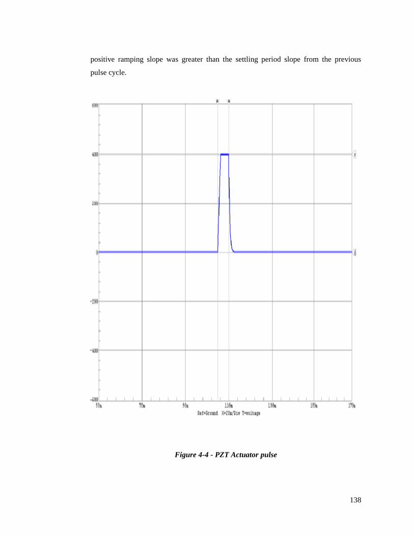
138
positive ramping slope was greater than the settling period slope from the previous
pulse cycle.
Figure 4-4 - PZT Actuator pulse

139
4.4 Signal and Data Processing Technique
The open-loop micro-pump characterization was performed using an internal
hardware based software algorithm (Figure 4.5) and an externally developed application
specific software package.
Figure 4-5 - Hardware based software algorithm flow diagram
OpticalFiltering
PhotonicConversion
FrequencyCounter
InterferometricMeasurement
TriggerDetection
DriectionDecoder
External Data Captureand
Oscilloscope MonitorInterface
N-samplebuffer
FringeDecoder
TimeDivision
Positioning
N-countbuffer
N-fringebuffer
N-alignmentbuffer
DisplacementAlgorithm
N-Displacementbuffer
SPIFramer
AnalogConvertion
SPIbuffer
DataTransfer
Algorithm

140
Initially, the amplitude of the PZT pulse was measured against the modulation
frequencies to determine the level of filtering that had to be applied without loss of valid
data.
The modulation waveform was converted using photovoltaic trans-conductance
synthesis. The number of samples taken over the modulation waveforms governed the
accuracy of the conversion process and, in this case, it was one million samples per
second (1 Msps).
4.5 Photonic Conversion Extraction
The interferometric measurement data was delivered optically and then
converted to electrical potentials (Figure 4.6). Even at this point, the software
controlled the temperature drift offsets associated with the fibre elements delivering
both the modulation fringes and the reference signals to the conversion electronics. This
was achieved through the initial optical sampling without the modulation fringes being
present (no PZT actuation pulse).
Figure 4-6 - The dynamic Photonic conversion envelope
Bandwidth Breach Envelope Valid
Modulation Envelope

141
The effective noise envelope of amplitudes above the 20 mV and randomised
frequency was filtered down to a noise envelope of < 5 mV at the input to the trans-
conductance amplifier. The software employed a 16-tap low-pass FIR filter algorithm
that actively reduced the optically induced noise before the input modulations were
converted into electrical potentials.
The conversion software constantly monitored the signal to noise ratio and
subsequently acted on any amplitude changes associated with valid frequency
responses. For invalid frequencies (cycle to cycle variations > 350 KHz), the offending
cycle was discarded and a new cycle was inserted, based on the preceding and post
cycle’s paths (indicated in thick red line in Figure 4.6).
Figure 4.7 shows the software path of the photonic conversion algorithm. The
software allowed for variations in the optical noise spectrum as long as the output was
within the specified parameters of the frequency and amplitude envelope (< 350 KHz
and < 5 mV).

142
Figure 4-7 - Photonic Conversion Algorithm Block diagram (Appendix B.4.2)
Frequency & AmplitudeMonitoring
InterpolationAlgorithm
RoundingFunction
ConversionBuffer
FromOpAmp
> 350KHz,
> 5 mV
Yes
No
To TriggerDetection

143
Figure 4.8 demonstrates the usefulness of the FIR filter, showing the output
almost perfectly reconstituted from a very high ambient noise and a 2 KHz sinusoid of
±100 mV amplitude presented to the input of the acquisition amplifiers.
Figure 4-8 – Model-Sim Result for Input Modulation Using FIR Filter
2.0 ms 4.5 ms 7.0 ms
2 KHz Filtered
output
±100 mV, 2 KHz sinusoid +
ambient noise
FIR add & accumulate
loop counter
Sampling clock

144
4.6 Displacement and Trigger Detection Method
The trigger for the displacement acquisition was identified using a software
process called the Iterative Amplitude Frequency Sampling (IAFS). This level and
frequency of the response was continuously monitored for dynamic variations that met
the preset conditions considered as the valid trigger points, which initiated the data
sampling for the incoming displacement modulations. The amplitude levels were set
between 50 mV and 100 mV, while the frequency was between 1 kHz and 2 kHz. The
frequency was for the positive deflection of the PZT actuator, and the negative
deflection was between 2 kHz and 4 kHz.
Figure 4.9 shows the software process used to extract the valid data acquisition
trigger between each successive actuation pulse being generated (Appendix B.4.3).
Figure 4-9 - Trigger Detection firmware process
The trigger outcome also produced data that was further screened for the
direction of the displacement, as described in Section 3.4.21.
AmplitudemonitorFrom
ConversionBuffer
TriggerVali d
Frequencymonitor
AmplitudeTable
FrequencyTable
No
AmplitudeNormalizer
Frequencyfitter
Yes
Start
Yes
No
Yes
No
No

145
4.6.1 Direction Decoder Considerations
The direction decoder took the trigger data and, by relative positioning with
respect to the actuation pulse, along with the extracted frequency, the direction of the
displacement was determined. The relaxation of the actuator diaphragm after each 5 ms
pulse was sufficient to measure a low frequency decaying dampening effect that could
be used as a reference marker preceding the next actuation pulse. Since the actuation
pulse ramped up at a predetermined slope of approximately 20°, and the response was
predictable for the duration of the ramping slope, a set of frequency coefficients were
compared with the continuously sampled incoming interferometric data stream and
when a match occurred, the upward displacement was determined (Appendix B.4.4).
Similarly, the downward displacement was also checked, except for the actuator pulse
slope declination being 40°.
4.6.2 Frequency Counting Method
Frequency counting occurred over the modulation fringe data that had been
normalised and stripped of erroneous information. The frequency extraction algorithm
(Appendix B.4.5) followed the process described in Section 3.4.20. The frequency was
extracted using peak-to-peak time markers where each cycle was proportional to the
wavelength of the light source, which was 632.8 nm and, when combined with the time
constant, produced an accurate frequency measurement. The frequency counting
function is given in Appendix B.4.5. Fringe decoding was simply frequency counting
except for the inclusion of the wavelength constant and the cycle error coefficients
(Figure 4.10).

146
Figure 4-10 - Fringe Decoder Process
The portion of unresolved cycle sampled was always decimated in the time
division proportional to the ratio of the final over the interpolated cycle count multiplied
by the wavelength of the laser source, as depicted in Equation 27:
Equation 27 λ×= −−
T
tTnf C
CD )(
)1(
Where
Df(n-1) is the displacement for a portion of unresolved modulation cycle
C(T-t) is the portion of incomplete modulation cycle time
CT is the complete modulation cycle time.
The software algorithm resolved the Df(n-1) portion of the incomplete cycle,
appending the fraction to the sum of the accumulated fringe decoded displacement.
On completion of the fringe counting and decoding process, the positioning of
the displacement points had to follow the terminal position of each interpreted cycle. In
other words, for each frequency cycle, the final CT time was where the fringe
interpolated displacement point was located. By extraction of a single point for each of
the fringe cycles, the displacement could be a straight line of specific amplitude (sum of
preceding displacement points), but of varying time divisions. By stacking the
displacement points end-to-end, and then interpolating between them using the time
CounterFrom
FrequencyBuffer
Wavele ngthConstant
X
+
-
DirectionFinder
ErrorConstant
FringeBuffer

147
division multiplexing, the displacement data was then generated and saved in a buffer
(Appendix B.5.1).
A displacement algorithm (Figure 4.11) converted the data into its analog
equivalent digital components that could be ported through a digital-to-analog interface
as well as retained in a buffer for serial transmission to an external device, such as a PC
or any other compatible data acquisition device.
Figure 4-11 - Displacement Software Block diagram
Start
Samplingtrigger
≥8 mV?
DirectionUp/Down
Yes
No
Yes
Up
Down Ignore & ReadNext
Count betweenMaximum
points
Stop
ADC InputSaveADCData
Read Data
Frequency<350MHz
ExtractMinimums and
Maximums
No
SaveCount
Read Count
Cnt x+(Wave length)
Cnt x-(Wavelength)
SaveDisplace-
ment
DACOutput
Oscilloscope
ReadDisplacement
CycleComplete
Reset Buffers& Pointers
Yes
NoSTOP
?
Yes
No
SPIPort
PCStorage
148
The format was maintained for cycle-to-cycle comparisons used in subsequent
closed-loop operation in Chapter 4. The code can be viewed in Appendix B.5.1. Figure
4.11 represents a complete data capture and displacement detection functional block
diagram as used for the open and closed-loop micro-pump experimentation. An
amplitude trigger that initiated an intermediate up and down directional determination
function started the data acquisition. The subsequent processing produced the final
displacement that was saved in a digital format. The same data was then passed through
a D/A converter for direct oscilloscope connection. This was useful for verification
purposes when compared directly to an alternative form of measurement (i.e., non-
contact pressure or capacitive sensor).
The initial capture buffer was a window of 10ms bandwidth, sampled every 1µs
seconds and 10K words deep. In total, 2.56Mbits, captured via a parallel interface and
sampled every 6.25µS, was processed through the ADC interface buffer prior to being
passed through FIR filters. At most, a latency of approximately 16µS was introduced
using 16 registers in a synchronised pipeline. This delay was required while the
processor manipulated the data prior to passing it on to the FIR filter coefficients table,
which was used as a comparison with the previously captured data set. This was useful
in determining a level of accuracy during the micro-pump operation. Subsequently, it
was used for error correction in the feedback, closed-loop arrangement where additional
buffers were introduced to handle the feedback loop coefficients needed during the
progressive accumulative sampling. Each sample was stripped of unnecessary bits that
were randomly generated as noise during capture, when passed through the FIR filter
algorithm. In some cases the removed bits are substituted by interpolation over the
randomised time window.

149
4.7 Closed-loop Control Methodology
PZT actuators could be operated in both the open and closed-loop applications.
Normally, the displacement of the actuator, in open-loop operation, corresponded to the
drive voltage but, at the same time, a high degree of accuracy could not be achieved
because open-loop PZT actuators exhibited the hysteresis and creep behaviour, common
to open-loop positioning systems. Closing the loop on the actuator was necessary for
high linearity, long-term stability, repeatability and accuracy. To this end, some PZT
actuators were equipped with position measuring systems providing sub-nanometer
resolution and larger bandwidth. The output voltage driving the PZT actuator was
controlled by comparing a reference signal to the actuator feedback signal, extrapolated
by an interferometer as varying frequency fringes up to 300 KHz, depending on the
propagation delay of the driver voltage.
It was determined that a piezoelectric actuator could attain its nominal
displacement position in approximately 1/3 of the period of the resonant frequency.
Rise times in the order of microseconds were possible. Unimpeded by load, such
devices could readily achieve very high speeds, but as soon as the pressures exerted in
the micro-pump chambers loaded the piezoelectric element, the resonant frequency
would be decreased as a function of the square root of the mass (i.e., quadrupling the
mass will halve the resonant frequency). Piezoelectric actuators were not designed to
run at the resonant frequency, with full stroke and load, because the resulting high
dynamic forces could damage the structural integrity of the ceramic material. It was
possible, however, to control the amount of potential applied to the piezoelectric
actuator in a closed-loop system, at carefully metered levels, delivering only the amount
of force required to exert enough pressure and deliver a predetermined amount of liquid
or gas to the output.
At the time this Doctoral research commenced, there was no research uncovered
in the literature review of micro-pump structures that utilised a fibre optic
interferometer in the sort of configuration depicted in this research. However,

150
interferometer displacement measurement had been used for precisely measuring the
surface characteristics of materials and micro-pumps, but not to serve as a sensor
feeding back information in order to close the loop in a free running micro-pump.
The closed-loop control of a micro-pump, based on the actuator displacement,
was therefore a novel idea but only had practical application if the final closed-loop
system could be integrated onto a single platform. At the time this research commenced,
this was a considerable task, given the state of technology in the field of polymer optics
and microelectronics at the time. However, there was some literature uncovered
suggesting that this integration was possible.
The basis for closed-loop operation of the micro-pump, as in other control
applications, was in the ability of the system to affect the open-loop characteristics if (or
when) the dynamic parameters were in some way altered. There were also some micro-
pump configuration applications where it was possible that the closed-loop would not
need to be invoked. This would occur if the steady state operation of a micro-pump was
not in any way altered by adverse conditions of the environment or the impurities in the
processing of the pumping media.
4.8 Micro-pump Closed-loop Experimental Considerations
The micro-pump characterisation took into account the structural, mechanical,
chemical and electrical parameters that were susceptible to steady-state variations
attributable to electrical noise, temperature, vibrations, inductance, capacitance and
chemical reactions. In a closed-loop control system the performance is measured by its
steady-state error, gain and phase margins, which are essentially the criteria for
optimality. The performance and reliability of a micro-pump is only as good as its
feedback compensation, which maximises or minimises the performance index which,
in turn, is largely unknown until the completion of the optimising process. Figure 4.12
illustrates a simple adaptive control system for a micro-pump with varying parameters
that are continuously measured and then compensated so that the system performance
criteria are always satisfied.

151
Figure 4-12 - Micro-pump feedback control system
When considering a closed-loop system for a micro-pump, it was imperative that
the chosen design parameters closely matched the ideal responses to minimise the
performance index or the error between the actual and ideal response.
4.9 Closed-loop Controlling Elements and Parameters
The closed-loop (feedback) control system for the micro-pump was composed of
three components (Figure 4.12):
• A piezoelectric actuator
• Fibre optic interferometer (sensor)
• Control logic.
The characterisation process investigated a number of functional parameters,
such as frequency, amplitude and phase that dynamically influenced the operational
Self - priming membrane micro-pump
Microelectronic Control Logic
AMP Detectors
PZT quadrature phase lock
PZT pump actuator
CPLD
ADC
Fibre Optic Interferometer
PZT stretcher
DC2 Laser
signal
ref
ere
P L
P S
P M
P R
D
C1
DAC Driver
DAC Driver
IN OUT

152
characteristics of a micro-pump. The free running open-loop response generated a set
of coefficients that characterised the micro-pump’s steady state operation. Applying a
set of adaptive algorithms, over each micro-pump actuation, and overlaying the data
with the previous sample, generated a set of error coefficients, which closely matched
the steady state response for a given frequency, phase, amplitude and pumping medium.
To understand the feedback in a closed-loop system, a frequency response
analysis is important, as it is the primary element elicited by the direct affect on the
actuator. The frequency analysis could show how a disturbance of the input affected the
control and, ultimately, the performance of a micro-pump. For any system variations at
the input, the feedback control loop had to have sufficient time to absorb its effect
before the actuation controller variables were influenced to affect a change in the
steady-state operation of the system. This was not always the case, however, and
unwanted variations in frequencies that managed to propagate through to the controller,
and influence the performance variables, were mapped from cycle to cycle.

153
4.10 Control Logic and Transfer Function Considerations
The control logic was composed of microelectronic circuits capable of manipulating
the parameters of the micro-pump controlling elements. The intelligence for the control
logic was implemented in the form of a digital signal processor (DSP).
Figure 4.13 shows a basic block diagram of an adaptive control system that was
used to optimise the performance of the micro-pump.
Figure 4-13 - Block Diagram of an Adaptive Micro-pump Control System
All of the parameters, which were known to vary with time in the block labelled
“Parameter optimization”, were continuously measured at input A and output C of the
piezoelectric actuator block in order to identify the parameters requiring adjustment in
the control elements block to satisfy system specifications. Included in the Parameter
Optimization block were the fibre optic interferometer parameters.
Additional sensors were also included in the closed-loop, specifically thermistors,
accelerometers, piezo-resistors, capacitive or flow rate sensors, keeping in mind that
they could not be allowed to significantly alter overall system performance. When using
Control elements
(G1)
Piezoelectric actuator
(G2)
Parameters optimisation
(G3)
-
Controlled displacement
Ideal actuating level
Control variable Actuating signal
I A
B
+
Compensation coefficients
(H2)
C +
+ E
Elements optimisation
(H1)
+ D
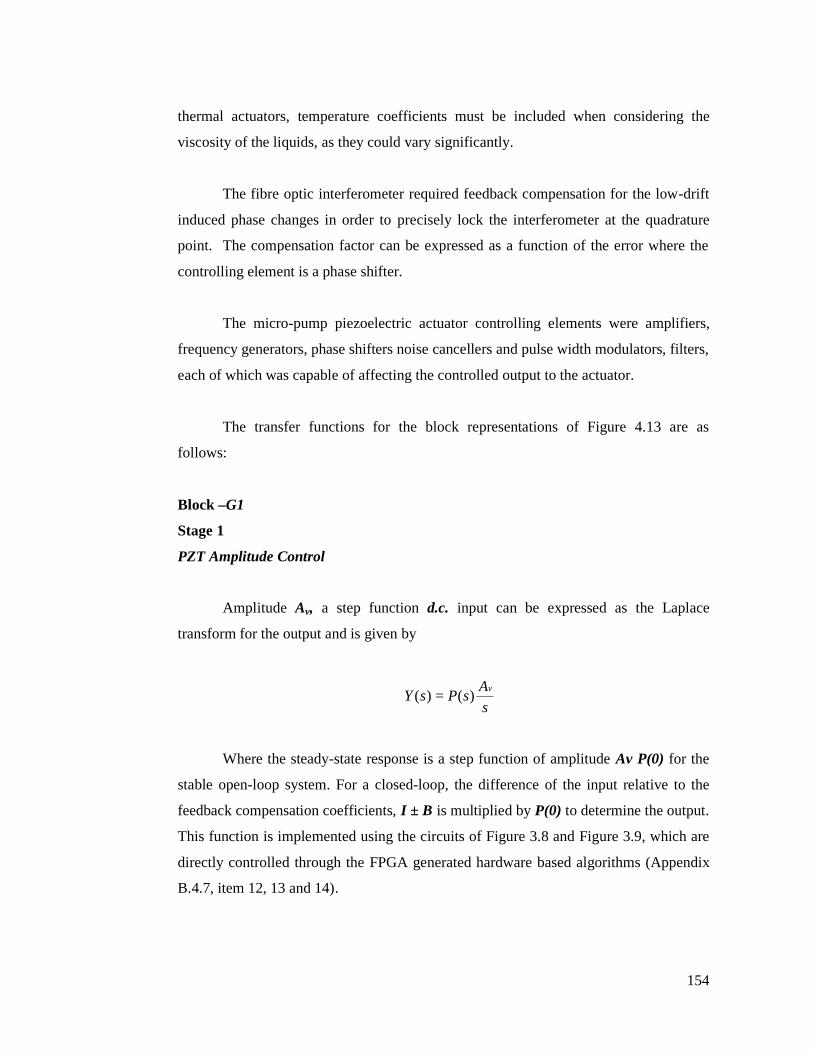
154
thermal actuators, temperature coefficients must be included when considering the
viscosity of the liquids, as they could vary significantly.
The fibre optic interferometer required feedback compensation for the low-drift
induced phase changes in order to precisely lock the interferometer at the quadrature
point. The compensation factor can be expressed as a function of the error where the
controlling element is a phase shifter.
The micro-pump piezoelectric actuator controlling elements were amplifiers,
frequency generators, phase shifters noise cancellers and pulse width modulators, filters,
each of which was capable of affecting the controlled output to the actuator.
The transfer functions for the block representations of Figure 4.13 are as
follows:
Block –G1
Stage 1
PZT Amplitude Control
Amplitude Av, a step function d.c. input can be expressed as the Laplace
transform for the output and is given by
sAsPsY v)()( =
Where the steady-state response is a step function of amplitude Av P(0) for the
stable open-loop system. For a closed-loop, the difference of the input relative to the
feedback compensation coefficients, I ± B is multiplied by P(0) to determine the output.
This function is implemented using the circuits of Figure 3.8 and Figure 3.9, which are
directly controlled through the FPGA generated hardware based algorithms (Appendix
B.4.7, item 12, 13 and 14).

155
Stage 2
Frequency and Phase Control
Frequency Fi, a steady state response for an input x = Asin ωt has a transfer
function P(s) and is given by
)sin(|)(|)( φωω += tjPAxFi
where )(arg ωφ jP= is the phase angle and |P(jω)| is the magnitude of P(jω).
The Laplace transform of the output can then be expressed as
)(*)()( sXsPsF =
22)()(ω
ω+
=s
AsPsF
In this case the phase margin is also considered, which is a measure of relative
stability. The frequency and phase of the PZT actuator is dependant on the feedback
path compensation coefficients (Appendix B.2, closed-loop files, CH1 contains the data
relating to the transfer function).
The feedback transfer function H2 is defined in terms of the systems sensor
input, which in this case the fringes are when the actuation pulse is applied. The element
of the transfer function are divided into a number of stages that are fixed and can not be
changed, in which case a feedback compensation is introduced.
In the real system, the frequency is controlled using hardware synthesized in the
FPGA (Appendix B.4.7, D:\SCHEMATICS\FPGA\BLOCK, Item 16).

156
Block – H2
Stage 1
Sensor Input Current Mode Amplifier (Trans-conductance function)
Since the function is current (i) driven and is frequency specific, the relationship
is expressed as follows
iKzVo =
where Kz is a gain factor composed of a reactance
fCf
Xcπ2
1=
and a feedback resistance Rf.
Combining the active feedback components Vo relative to the frequency specific
input can be determined.
)//( RfXciVo =
RfXcRfXciVo
+•
=
substituting for the active elements, we get
fCfRf
RfiVoπ21+
=
Note that the increase in the reactive element C, reduces the bandwidth of the
response and also the output voltage.
Converting to a Laplace transfer function equivalent

157
Ks
KsisYω+
=1
)()(
Stage 2
Signal Conditioning Voltage Mode Amplifier
Once converted from the photovoltaic input to voltage, the signal conditioning
must incorporate some kind of a voltage pre-amplifier stage that will eliminate the
unwanted elements by a way of a filtering system that may include a Low-pass and
High-pass combination.
The transfer function for the voltage output can be expressed as follows
+
+•=fCfRf
RfViVoπ21
1
again, the Laplace equivalent is
++•=
KsKsVsYω1
1)()(
Stage 3
Signal Conditioning (Low-Pass Filter)
This stage incorporates a low-pass filter (sixth-order) filter for which the transfer
function can be defined as:
++
•
−
++
•
−
++
•
−
=
111
)(
3
2
32
2
21
2
1 cccccc
LP
fjfQ
fCf
fjfQ
fCf
fjfQ
fCf
KfH

158
where K is the gain factor and each stage gain, Ka•Kb•Kc, fc is the -3 dB point and C1 to
C3 are the filter coefficients (constants) at which the filter output is stable. These
coefficients are stored in the tables as generated with the FIR filter algorithm in
Appendix B.4.7, D:\SCHEMATICS\FPGA\VHDL item 3. The Q factor is also a
derivative of the gain controlling elements and is normally characterised for a filter type
such as Bessel, Chebyshev or Butterworth. All of these coefficient were stored in tables
located within the embedded memory blocks of the FPGA devices. In some of the cases
where the noise from the frequencies below 60 Hz (predominantly when the initial
experimentation was undertaken in a confined laboratory area), was considerably high,
a High-pass filter was introduced and an additional transfer function was incorporated
into the H2 feedback loop as stage four.
Block G3 represents the functions for an ideal PZT actuator operation follows
the same transfer functions and is controlled using the elements such as amplitude, pulse
width, unit ramp and frequency as depicted in the block G1. The function is given as
)(arg1)( 222 sPsss
AsF •+
••=ω
ω
where each stage effecting the ideal system parameters is multiplied by the preceding
output. The ideal PZT actuator in a real system is extrapolated from the lookup tables,
which are based on the normalized set of values for a particular medium used
(Appendix B.2.15).
Block G2 is the actual PZT actuator function, which is driven by the results of
the control block G1 elements. The function is predominantly the same as that of G3,
except that the coefficients feeding the variables such as amplitude, phase and
frequency are those derived from the feedback transfer loop function H2 and H1.
Block H1 is a transfer function representing the PZT actuator error constants
that are generated to optimise for loses in the active control elements of block G1. This
is implemented in the software of the system (Appendix B.5.1).

159
The frequency response transfer functions, relating to the amplitude of the system
ratio for any of the stages in the closed-loop could be obtained implicitly since the input
and output have the same frequency (Equation 28). In the case of our analysis, the input
was generally affected by the passive components that were used to stabilise the
operations of any number of functions. Usually, these were resistors, capacitors and
inductors. In addition, amplifier characteristic transfer functions were incorporated as
separate stages evaluated as the feed-forward or feedback boosters or attenuators. The
circuit functions are summarised by transfer functions designed to meet the circuit
specifications. In the case of resistor and capacitor (RC) networks (Figure 4.14), which
were used to filter or attenuate signals, the transfer function frequency response is given
by:
Equation 28 i
o
VV
fG =)(
=12
1+fRCj π
Figure 4-14 - RC Network Circuit
If we consider the capacitive impedance denoted by:
XC = fCπ21 (Reactance)
R
C Vi Vo

160
and the linear resistance through R, it is possible to calculate the response of the
modulation frequencies on the basis that sinusoids are generated by summing of two
complex exponentials of opposing frequencies. It is shown that the magnitude of the
modulation fringe sinusoids are symmetrical, such that the negative part of the centre
frequency is mirror imaged with a positive equivalent: |G(f)|=|G(-f)|, whilst the phase
has odd symmetry: ))((()(( fGfG ∠−=−∠ . These properties apply to all transfer
functions associated with the circuits in outlined experiments and it was found to be
unnecessary to plot the negative frequency component because its symmetry to the
positive frequency.
The magnitude of the amplitude equals 0.707 or 2
1 of its unity gain at f = 0,
when
12 =fRCπ
and the centre frequency
RCf c π2
1=
that defines the operating band boundary between the two ranges (Figure 4.15).
Figure 4-15 - Magnitude Transfer Function
It has been shown that for frequencies below the centre frequency fc, the RC
circuit of Figure 4.14 does not drastically alter the amplitude of the complex exponential
input source, whilst for the frequencies greater than centre frequency fc, the same circuit
1 -1
|G(f)|
1
0.707
RCπ21
RCπ21
−
0 f

161
greatly attenuates the amplitude and subsequently reducing the output to well below the
input source. Similar transfer functions apply for the amplifier gain, where an integrator
is used to attenuate over a range of frequencies above the bandwidth limitation of the
amplifier.
It has been shown that the cut-off frequency is only dependant on the products of
the resistance and the capacitance. The phase shift caused by the RC circuit in Figure
4.14 is shown in Figure 4.16.
Figure 4-16 - Phase of Transfer Function for RC Circuit of Figure 4.4
It can be seen that at the phase shift at the cut-off frequency (fc) is:
−
4π
and below the cut-off frequency (fc), it is small and can be omitted from consideration,
but at the higher frequencies, the phase shift is substantial enough to alter the
characteristics of the equation by a factor of:
−
2π .
1 -1
|)(| fG∠|G(f)|
-Π/4
0 f
-Π/2
Π/2
Π/4
RCπ21
−
RCπ21

162
The phase shift of the RC circuit of Figure 4.14 corresponds directly to the
difference between a cosine and sine. Knowing that a sinusoid is the sum of two
complex exponentials, each having a frequency equal to the negative of the other and
since the circuit is linear and if the source input is a sine wave, we know that the
modulation fringe input is:
)2sin()( ftAtVin π=
Equation 29 ( )ee ftiftiin i
AtV )2(2
2)( ππ −−=
Since the input is the sum of two complex exponentials, the output must also be
a sum of two similar complex exponentials. The complex amplitude is the only
difference, since it is multiplied by the transfer function evaluated at each exponential
frequency.
Equation 30 ee ftiftiout fG
iAfG
iAtV )2(2 )(
2)(
2)( ππ −−−=
The transfer is most conveniently expressed in polar form and so the output
voltage simplifies to
Equation 31 ee fGftifGftiout fG
iAfG
iAtV ))((2())((2 )(
2|)(|
2)( ∠−−∠+ −−= ππ
The circuit output as well as input is sinusoidal, having a gain equal to the
magnitude of the transfer function evaluated at the source frequency and phase equal to
the phase of the transfer function at the source frequency. This is true for all the
modulation frequencies that are captured and evaluated for their amplitude and phase
for each of the cycles. Since the data capture algorithm processes each cycle
individually, the linear equation as described by Equations 29, 30 and 31 is applicable.
The evaluation of the amplitudes, frequencies and phases for the modulation fringes in a

163
closed-loop system allows for latency induced error correction, as long as the effective
delay does not exceed the pipelining for the functional processing.
A number of register or memory based delay pipes were implemented as
required in order to maintain the data flow through the feedback control system. Each
time a measured frequency was compared with the frequency of the previous input, the
difference either increased or decreased the slope of the actuator driver voltage,
effectively altering the potential to the PZT actuator, which consequently increased or
decreased the displacement frequency. This type of affect on the actuator had an
associated latency that propagated through the system since the electronics were fully
synchronised and retimed to meet the specified output requirement.
The bulk of the signal processing was included in the Parameter Optimisation
block, passing only the error signal to the Control Elements block where the
appropriate elements were modified, and output to the piezoelectric actuator block fully
optimised (Section 5.5). The compensation coefficients, denoted by B (Figure 4.17),
influences the frequency and amplitude of the actuating signal by a way of an adaptive
process, which is linearly proportional to the displacement during data capture in real-
time processing.
Figure 4-17 - Transformation of the Control System Function
The forward transfer functions for the system are represented by G1, G2 and G3,
while H1 and H2 are the feedback transfer functions. The closed-loop transfer function
( )
11
321
1 HGGGG
−+
- I +
2H
C E
B

164
is defined as C/I (Figure 4.18) and the actuating signal ratio as E/I, while the primary
feedback ratio is B/I.
Figure 4-18 - Equivalent block function
Each of the elements of the system is modelled and represented by a transfer
function and a frequency response. In an open-loop analysis of the system, the transfer
function is fixed with a finite number of constant parameters, which when compared
with the actual parameter values exhibited during the operation of the system produce a
deviation reflecting the accuracy of a response. This is a measure of the sensitivity of
the system as represented by the transfer function that differs from the constant
parameters chosen.
The frequency response function of the system can be represented from the
transfer function of the system by adjusting the complex variables within each of the
transfer function blocks, as represented in Figure 4.16. The steady-state frequency
response of a stable system where the interferometric modulation input is represented by
the function:
Equation 32 )sin()( φω += ttf
and the Laplace Transform is given by;
Equation 33 22
cossin)(ω
φωφ++
=s
ssF
( )( ) ( )322111
321
1 GGHGHGGGG
+−−+
I C

165
where, s is a complex variable denoted by ωσ js +≡ , real variables σ and ω.
The closed-loop and feedback effectiveness in a generally stable system such as
this one is measured in terms of error constants and sensitivity. The error constant
system algorithm quantifies the measure of the steady-state error between the input and
output, while the sensitivity is a quantitative measure by which the overall transfer
function of the system is altered from the nominal value with changes to any of the
controlling elements. This is achieved by the use of non-linear differentiation over the
sampled modulation fringes and also over the actuator displacement. The differentiation
over the modulation fringes is used to extract the maximum and minimum points of the
frequency, and also to detect any impulse variations that indicate the displacement
direction change. For any output that is changing rapidly, overshoot or undershoot may
be a real problem. In that case, we can reduce the size of the change suggested by the
proportional controller. The derivative at the current time is simply the change in value
from the previous sample to the current one. This implies that we should subtract a
change of:
AD* (current - previous)
where AD is a constant derivative gain.
Each of the previous samples is progressively stored in memory and can be
extracted randomly during any of the interactive processes. In practice, proportional-
derivative (PD) controllers work well. The net effect is a slower response time with far
less overshoot and ripple than a proportional controller alone.
The feedback-processing algorithm was implemented in hardware using DSP
blocks. The blocks were composed of phase, frequency and amplitude elements
parameterised and referenced to tabulated coefficients.

166
4.11 Analysis and Control Electronics
The central processing unit interfaced with a number of peripherals, such as the
photo detector module, memory expansion card and the piezoelectric actuator driver.
Signal processing was achieved using a fast hardware algorithm that was dynamically
configurable during the real time operation of the system. Data transfer was achieved
through a couple of serial communication ports and the configuration of the hardware
was made possible through the In-System-Programmable (ISP) port during power-up by
the use of a serial programmable read only memory (PROM) device. The digital signal
processing functions, such as finite impulse response filters (FIRs), Fourier analysis,
convolution, differentiation, integration averaging, phase shifting, and signal smoothing
were implemented in a complex programmable logic device (CPLD) during the real
time operation. Sampled data was stored after processing for each of the amplitude-
triggered cycles, and then compared with the previous sample to determine the error
coefficient required to control the piezoelectric actuator elements in the next sample.
The experimental results for this research were obtained using the central
processing module. First, data was accumulated at a rate of 1 Mbps and stored in an
array of 100 samples, allowing for progressive averaging and filtering over that period.
The samples were then differentiated for maximum and minimum turning points and
relative phase angles. The resulting slopes were analysed for amplitude reference
crossings, with peak amplitudes extracted and digitised, generating a clock with a
frequency proportional to the captured interferometric fringes. Sampling was continuous
and referenced to predetermined frequency variations (as described in Chapter 3), which
determined the displacement direction with a latency of 100 samples (100 µs).
Displacement was calculated over a complete actuating cycle having an “ON”
period of T = 5 ms and “OFF” period dependant on the pumping frequency, and since
the ratio of the duty cycle was variable, the elements of the lead compensator (closed-
loop feedback parameter) can be modified to satisfy system specifications based on the
adaptive control requirements.

167
In order to satisfy the open-loop requirements for a steady state response, the
sum of integrals, or the area of the displacement was correlated with the preceding
samples, and the variations were used as error coefficients for adjustments within the
lead compensation elements of the system. The area integral for the displacement can
be expressed as
Equation 34 ∑ ∫−
=N
tn
1tn
udtArea
where, u = f(t) between the t axis and the ordinates at tn-1 and tn, which are the subset
samples.
Using digital interpolation, the area integral can be expressed as
Equation 35 ( )( )2
ttuuttuf(t) n1)(nn1)(nn1)(nn
n −−+−=
++
+
By applying a systematic block diagram reduction for the multiple feedback
loops into canonical form, the overall algorithm for the adaptive displacement could be
simplified considerably, as demonstrated in Figure 4.17 and Figure 4.18.

168
4.12 Displacement Verification Method
In order to verify the displacement measurement obtained using a fibre optic
interferometer, a comparison with a capacitive proximity sensor displacement
measurement was made, which also related to the flow rate of the micro-pump at a set
frequency and pulse shape. The method, as shown in Figure 4.19, illustrates the
experimental arrangement that was used for this verification process. The flow rate was
determined by the use of the mass method, where the medium being pumped was
weighed prior to being processed, and then reweighed after a predetermined pumping
time. The receptacle, containing the mass of the fluid pumped had to be equal to the
initial sample weight, minus the weight of the initial sample after pumping at a given
frequency, amplitude and pulse shape.
Figure 4-19 - Capacitive sensor displacement measurement set-up
The flow rate measurement was taken over one minute, at which time the weight
of the piped sample was converted to litres, since the initial sample of precisely
PZT Driver & Sensor Amplifier
PZT(+) CDS(+) S CDS(-) PZT(-)
Weighing Scale Initial Sample
Weighing Scale Pumped Sample
Micropump
Receive Container
SupplyContainer
Capacitive Displacement Sensor

169
measured fluid (2ml) was weighed before being pumped. The experiment was carried
out over a number of pumping frequencies and amplitudes, just as for the fibre optic
interferometer configuration to which it was compared. The displacement was related to
the flow rate by considering the amount of fluid transferred through the micro-pump
chamber during a single actuation pulse. Due to the preset width of 5ms for the
actuation pulse, a maximum frequency used was 100Hz, which allowed for a 50/50
cycle to be applied. Higher frequency could be applied, but the settling of the diaphragm
between the pulses would not be dampened enough to completely close the valves
before re-actuation. Figure 2.0 shows the transient response for the displacement fringes
when the actuation pulse is at zero potential, which is expressed in the following form
for the first-order system,
Equation 36 tAe ατ −=
where τ is the time constant used to measure the settling time and
Equation 37 tAe dt ωτ α sin−=
for the second-order system (α > 0)
where α = ζωn is the damping coefficient and 21 ζωω −= nd , which is referred to as
the damped natural frequency. α is the inverse of the time constant τ of the system and
can be expressed as τ =1/ α. Assuming that the damping ratio ζ is 0 ≤ ζ ≤ 1, the unit
step-response of an underdamped second-order system can be expressed as;
Equation 38 tet dt
d
ωω
ω α sin1)( −=
By substituting the data for the portion of the time as obtained for 28% glycerol + water,
the settling time Ts, or ω(t) reached its steady state within 2 to 4 percent of its final
value, in this case 1.3 ms (Figure 4.20).
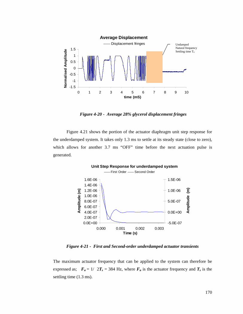
170
Average Displacement
-1.5
-1
-0.5
0
0.5
1
1.5
0 1 2 3 4 5 6 7 8 9 10time (mS)
Nor
mal
ised
Am
plitu
de
Displacement fringes
Figure 4-20 - Average 28% glycerol displacement fringes
Figure 4.21 shows the portion of the actuator diaphragm unit step response for
the underdamped system. It takes only 1.3 ms to settle at its steady state (close to zero),
which allows for another 3.7 ms “OFF” time before the next actuation pulse is
generated.
Unit Step Response for underdamped system
0.0E+002.0E-074.0E-076.0E-078.0E-071.0E-061.2E-061.4E-061.6E-06
0.000 0.001 0.002 0.003Time (s)
Am
plitu
de (m
)
-5.0E-07
0.0E+00
5.0E-07
1.0E-06
1.5E-06
Am
plitu
de (
m)
First Order Second Order
Figure 4-21 - First and Second-order underdamped actuator transients
The maximum actuator frequency that can be applied to the system can therefore be
expressed as; Fa = 1/ 2Ts = 384 Hz, where Fa is the actuator frequency and Ts is the
settling time (1.3 ms).
Undamped Natural frequency Settling time TS

171
5 Open and Closed-Loop Experimental Results

172
5.1 Open-Loop Overview
In the first experimental phase of this Doctoral research program, the open-loop
characterization of a piezoelectric micro-pump examined a number of parameters, such
as:
• Frequency
• Amplitude
• Pulse width
which could be used to precisely control the micro-pump operation. The closed-loop
control could be achieved by closing the loop using error coefficients generated from
the elicited evoked potentials, measured using a non-contact fibre optic interferometer.
This chapter documents the usage of the open-loop data to generate a set of
closed-loop transfer functions that produce the steady-state error coefficients. Herein, it
will be shown that an effective closed-loop feedback algorithm can be (and was)
developed utilizing these coefficients, which could be mapped into a dynamically
varying adaptive system.

173
5.2 Open-loop Experimental Outcomes
The following results show the relationship between the impulse modulation
fringes and the piezoelectric actuator displacement using a fibre optic interferometer.
Figure 5.1 illustrates how the intensity modulation fringe amplitudes and their
frequency components depend on the actuator peak driving voltage and its rate of
change.
Figure 5-1 - Piezoelectric Actuator Pulse and Displacement Elicited Modulation
Fringes
The steeper the actuator driving voltage slope (rate of change), the greater the
frequency and intensity modulation fringe excursions where Equation 25 governs the
bandwidth limitation. It can be seen that the velocity of displacement is fastest at the
steepest slope of the piezoelectric pulse.
Figure 5.2 represents a positive excitation fringe pattern for the displacement of
the micro-pump diaphragm when pumping water. Note the low frequency preceding the
high frequency fringe sinusoids that was used as a signature for the beginning of the
diaphragm displacement – this had a distinct and incomplete cycle transient function,
indicating a sudden change in the diaphragm position.
050
100150200250300350400450
0 1 2 3 4 5 6 7 8 9 10
Time (mS)
PZT
Ampl
itude
(V)
-0.6
-0.4
-0.2
0.0
0.2
0.4
0.6
0.8
Frin
ge A
mpl
itude
(V)
PZT Pulse Modulation Fringes
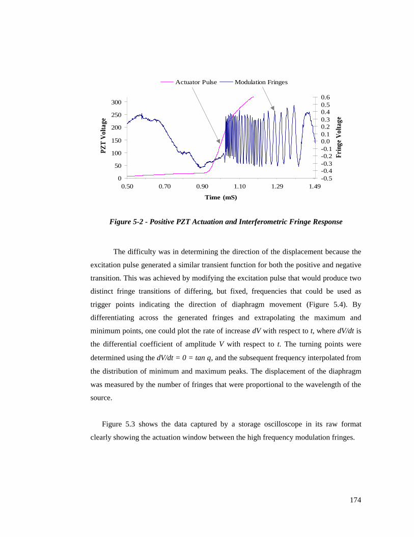
174
Figure 5-2 - Positive PZT Actuation and Interferometric Fringe Response
The difficulty was in determining the direction of the displacement because the
excitation pulse generated a similar transient function for both the positive and negative
transition. This was achieved by modifying the excitation pulse that would produce two
distinct fringe transitions of differing, but fixed, frequencies that could be used as
trigger points indicating the direction of diaphragm movement (Figure 5.4). By
differentiating across the generated fringes and extrapolating the maximum and
minimum points, one could plot the rate of increase dV with respect to t, where dV/dt is
the differential coefficient of amplitude V with respect to t. The turning points were
determined using the dV/dt = 0 = tan θ, and the subsequent frequency interpolated from
the distribution of minimum and maximum peaks. The displacement of the diaphragm
was measured by the number of fringes that were proportional to the wavelength of the
source.
Figure 5.3 shows the data captured by a storage oscilloscope in its raw format
clearly showing the actuation window between the high frequency modulation fringes.
0
50
100
150
200
250
300
0.50 0.70 0.90 1.10 1.29 1.49
Time (mS)
PZT
Volta
ge
-0.5-0.4-0.3-0.2-0.10.00.10.20.30.40.50.6
Frin
ge V
olta
ge
Actuator Pulse Modulation Fringes

175
Figure 5-3 - Digital Oscilloscope Fringe Modulation Capture
Note the oscillations start from a steady state potential of less than –0.15V with
a noise window of up to 25mV and remaining constant over the whole of 10ms
sampling window. The continuous low frequency modulations shown from 3.5ms to
7.0ms were proportional to the maximum level of the actuation pulse (400V) with a
gradient of approximately 1.2º. At 7.1ms, and until the 8ms time lapse, the change of
direction was determined based on the sudden onset of higher frequency modulations.
The low frequency dampening continued after the actuation potential was back to its
initial state of 0V and this was due to the settling of the diaphragm when the PZT
membrane was relaxed, which caused undulations of the diaphragm.
Figure 5.4 shows the capture of a single pulse, sampled and converted to its
digital equivalents.
time (seconds)
Am
plitu
de (V
olt)

176
Figure 5-4 - Digitised Fringe Modulations using the DSP Algorithm
During the positive transition of the applied PZT potential, a sudden change in
frequency was used as a trigger point for the initialisation of the displacement signal-
processing algorithm (Appendix B.4.4). Data was averaged over a number of samples
to filter out the high frequency noise modulated by the fringe coefficients. The
averaging distribution factor was determined from the amplitude of noise carried by the
fringe sinusoids. This was an adaptive function, calibrated during the manufacturing
process that could vary within a predetermined parameterised coefficients range (16 to
128 filter taps).
It was shown that the elements controlling the actuation slope parameters had to
be dynamically configurable in order to limit the bandwidth within acceptable
boundaries for optimum amplifier performance. The boundary limitations were pre-
programmed into the coefficient tables and used adaptively for characterization of the
displacement under different pumping fluids of varying viscosity. Ultimately, the
bandwidth limitations could result in lower ramping rates and subsequently lower
pumping rates, but a fundamentally more stable and accurate pumping medium.
The pumping medium viscosity and density determined the volume of material
that flowed through the pump chamber during each pump cycle. This was expected
during open-loop operation since piezoelectric actuators exhibit hysteresis and creep
behaviour (like any other open-loop systems) and when loaded, their dynamic
DIGITISED
-0.4-0.2
00.20.40.60.8
11.2
2.8 3.4 4.1 4.7 5.4 6.0 6.6 7.3 7.9 8.6 9.2
Time (ms)
Dig
ital
-200
-100
0
100
200
300
400
500
PZ
T V
olta
ge
Digitized Fringes PZT Driving Voltage
Nor
mal
ized
Dig
ital
PZT
Vol
tage

177
characteristics may be altered. One way of maintaining long-term position stability,
repeatability and accuracy is to include feedback control for the piezoelectric actuator.
Figure 5.5 shows three displacement samples for water, taken 32 periods apart using
identical experimental set-ups, sampled at 2Hz.
Figure 5-5 - Three Samples of Water Displacement Using Identical Experimental
Procedures (taken 32 cycles apart)
It can be seen that the waveforms do not necessarily follow exactly the same
path, and the variations might be attributable to impurities in the water or the membrane
valve’s behaviour, caused by the diodicity (i.e., the ratio of reverse to forward flow
direction) at the same flow rate.
Generally, diodicity is a function of flow rate through a combination of valves
and chambers, and is considered to be a quantitative measure of efficiency. In addition,
membrane stiffness, thickness and mass, bonded to the metal diaphragm along with the
piezoelectric driver elements, could also have added to the variation in the open-loop
steady state coefficients. There were many elements that contributed to the variations in
the membrane displacement, which only further demonstrated the need for a reliable
and efficient system.
0.0
5.0
10.0
15.0
20.0
25.0
30.0
2.80 3.44 4.08 4.72 5.36 6.00 6.64 7.28 7.92 8.55 9.19
Time (ms )
Dis
pla
cem
ent
(um
)
sample- 1 sample- 2 sample-3
Dis
plac
emen
t (µm
)

178
When pumping water with 60% glycerol added, the displacement was reduced
due to the increase in the viscosity, which had the effect of increasing the diodicity of
the system (Figure 5.6).
Figure 5-6 - Displacement when Pumping Water with 60% Glycerol
It was shown that for the same experimental conditions, the volume of fluid flowing
through the micro-pump chamber, during each pump cycle, was (as would be expected)
dependant on a fluid’s density and viscosity. Maximum displacement for water was
27.2 µm, with 28% glycerol added it was 21.9 µm, and with 60% glycerol it was
reduced to 15.2 µm, at an excitation frequency of 2Hz and a duty cycle of 1% “ON” (5
ms) to 99% “OFF” (495 ms). It was shown that the pulse repetition frequency driving
the piezoelectric actuator has the effect of linearly varying the amplitude of the
membrane displacement.
A number of pumping frequencies were plotted against the membrane displacement,
which showed a decrease in displacement with increase in frequency (Figure 5.7 and
Figure 5.8). The percentage drop from 2 Hz to 15 Hz is 2.2%, 2.6% from 15 Hz to 30
Hz and 3.4% from 30 Hz to 70 Hz.
W ATER with 60% G lyce rol
0
5
10
15
20
2 3 4 5 6 7 8
Time (ms )
Disp
lace
men
t (um
) Disp lacement

179
Figure 5-7- Three Displacement Waveforms for Water at Different Pumping
Frequencies
The displacement for each of the frequencies, recorded over one minute,
averaged an error variation in the order of 0.35 µm. The same effect was noticed for the
varying piezoelectric driver voltage. When the amplitude of the pulse was decreased by
only 30V, the slope of the displacement and the modulation fringe frequency was also
decreased, with the effect of reducing the total area per volume of the medium as
indicated in Figure 5.8, which shows the area of displacement for the period of each
sample, where the displacement decreases as the frequency of actuation increases.
This is useful since the variations in frequency and amplitude can control the
feedback loop elements that compensate for the variations in the steady state of the
open-loop system. The area acquired was compared with the previous area in each
successive sample and this served as a reference for the frequency and amplitude
compensation during the feedback loop analysis.
05
10
15
20
25
30
2.8 3.4 4.1 4.7 5.4 6.0 6.6 7.3 7.9 8.6 9.2
Time (ms)
Disp
lace
men
t (um
)
2 Hz 15 Hz 30 Hz 70 Hz

180
Figure 5-8 - Displacement Area for Samples Taken at four Frequencies
A normalised open-loop characterisation of the displacement could be tabulated,
which could then be used as a reference signature for the same type of micro-pump,
allowing for the design and development of intrinsic performance and reliability
monitoring on a fully integrated closed-loop adaptive system.
During each of the experiments for measuring the displacement for a given
pumping medium, such as water, or a percentage glycerol mixture, a flow rate
measurement was taken using the applied method for both the fibre optic interferometer
and the capacitive displacement sensors. The initial experimentation using 70Hz
actuation frequency and water produced a flow rate of 748µl/min, which equalled to
178nl/pulse. When considering the accumulative displacement of Figure 3.58 taken at 2
Hz actuation pulse, the flow rate was 19.6 µl/min. The error measured over a single
cycle for a predetermined period was calculated to be 1.28%, an average of 178 nl/min
at 70 Hz and was calculated to be 2.28 nl. This calculation was based on the maximum
displacement variations over a minute sampling period. Since the amplitude was
proportional to the flow rate through the pump chamber and the connecting inlet and
outlet channels, a drop in the amplitude was found to directly influence the amount of
0.000.020.040.060.080.100.120.14
2.80 3.44 4.08 4.72 5.36 6.00 6.64 7.28 7.92 8.56 9.20
Time (ms)
Are
a (u
m2 )
2 Hz 15 Hz 30 Hz 70 Hz
Disp
lace
men
t Are
a (µ
mse
c)

181
fluid passing through the micro-pump. In this case, a drop in the amplitude reduced the
flow rate when the frequency increased, which was found to be characteristic of the
actuation pulse potential drop due to the increased load switching. This is clearly
demonstrated in Figure 5.7 where the amplitude at 30Hz drops by 4.8%, which results
in a variation of 8.5 nl through the micro-pump chamber. By applying linear
interpolation over the frequency variation from 2 Hz to 70 Hz, a proportionality
constant of 0.046 was obtained for the displacement and flow rate (Table 5.1).
Actuation Frequency
(Hz) 2 15 30 70
Displacement
(µm) 27.20 26.6 25.9 25.01
Flow Rate
(µl) 19.4 150.5 306.1 751.3
Table 5.1 - Flow Rate / Displacement vs. Frequency data table
Figure 5.9 shows the variations in the displacement and flow rate when
stimulated using a range of frequencies (i.e., 2 Hz, 15 Hz, 30 Hz and 70 Hz).
Flow Rate & Displacement Vs Frequency(Water Sample)
23.524.024.525.025.526.026.527.027.5
2 15 30 70Frequency (Hz)
Disp
lace
men
t (um
)
0100200300400500600700800
Flow
Rat
e (u
l)
Displacement Flow Rate
Figure 5-9 - Plot of Flow Rate vs. Displacement and Frequency for water
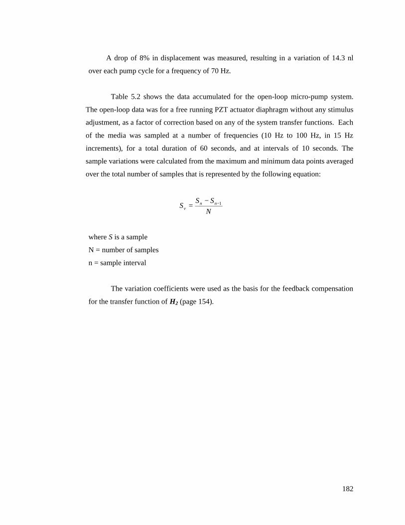
182
A drop of 8% in displacement was measured, resulting in a variation of 14.3 nl
over each pump cycle for a frequency of 70 Hz.
Table 5.2 shows the data accumulated for the open-loop micro-pump system.
The open-loop data was for a free running PZT actuator diaphragm without any stimulus
adjustment, as a factor of correction based on any of the system transfer functions. Each
of the media was sampled at a number of frequencies (10 Hz to 100 Hz, in 15 Hz
increments), for a total duration of 60 seconds, and at intervals of 10 seconds. The
sample variations were calculated from the maximum and minimum data points averaged
over the total number of samples that is represented by the following equation:
N
SSS nnv
1−−=
where S is a sample
N = number of samples
n = sample interval
The variation coefficients were used as the basis for the feedback compensation
for the transfer function of H2 (page 154).

183
Table 5.2 - Open-loop Response for Frequencies Ranging from 10 Hz to 100 Hz and
Four pumping media (air, water, water+28% and 60% glycerol)
The PZT driver stimulus was set at the maximum recommended by the micro-
pump manufacturer for optimum performance and load characteristics (400 V dc).
5.3 Open-loop Result Summation
The discrete component test system used during the experimentation described
in this section was designed and developed for the purpose of mapping the micro-pump
open-loop operational characteristics. Normally, commercially available equipment
such as PCs, data analysers, oscilloscopes, micro-scale displacement sensors
Medium Tested
Frequency Hz
OL MAX Total
Variation
OL MAX
% Variation
OL AVERAGE
Total Variation
OL AVERAGE
% Variation
OL MAX Disp. (um)
OL Flow Rate
(ul/min)
10 0.0806 11.36 0.0420 0.79 28.9225 0.0799 14.06 0.0421 0.81 28.2540 0.0791 11.71 0.0418 0.83 27.6055 0.0798 12.48 0.0421 0.85 26.9370 0.0812 12.58 0.0421 0.87 26.2585 0.0804 12.17 0.0420 0.89 25.61
100 0.0795 12.32 0.0418 0.90 24.9910 0.0539 10.81 0.0282 0.81 19.24 82.1925 0.0528 9.96 0.0280 0.82 18.81 200.9740 0.0538 12.77 0.0281 0.84 18.37 314.0355 0.0534 13.30 0.0281 0.87 17.91 420.9070 0.0535 14.23 0.0280 0.88 17.46 522.3785 0.0538 12.75 0.0281 0.91 17.05 619.14
100 0.0540 13.59 0.0280 0.93 16.63 710.7810 0.0399 10.99 0.0210 0.72 15.84 67.6725 0.0401 10.30 0.0209 0.73 15.47 165.2940 0.0412 11.21 0.0210 0.76 15.11 258.1855 0.0410 10.78 0.0210 0.78 14.74 346.3770 0.0409 11.84 0.0209 0.80 14.37 429.8385 0.0403 11.57 0.0210 0.81 14.02 509.19
100 0.0406 10.34 0.0209 0.83 13.68 584.4610 0.0305 11.90 0.0159 0.82 10.46 44.6825 0.0303 11.47 0.0160 0.85 10.22 109.1740 0.0305 12.31 0.0161 0.87 9.97 170.3555 0.0302 13.24 0.0160 0.90 9.73 228.6870 0.0306 12.43 0.0160 0.91 9.49 283.8685 0.0308 10.85 0.0160 0.93 9.26 336.31
100 0.0309 13.90 0.0160 0.96 9.03 385.96
AIR
WATER
GLYC28%
CLYC60%

184
(capacitive, optical, resistive and magnetic), laser drivers and highly sensitive trans-
conductance amplifiers would be considered adequate for such a task – however, these
elements were better suited to conventional analysis and verification, rather than
subsequent adaptive implementation, as was envisaged in this research.
The design of the test platform was undertaken primarily for the purpose of
dynamic versatility, integration and portability as it allowed for reliable performance
and repeatable outcomes. However, in using a discrete arrangement, the repeatability of
experimental procedures required continuous manual recalibration due to environmental
influences and interferences, purely on the basis of third party set-up procedures. This
was overcome by totally redesigning the test platform into a laboratory-on-a-board
system, using dynamically configurable electronics, where every aspect of the system
was accessible and controllable by the user. By having full access to all of the features,
parameters and elements of the system, an evolving environment was created that, over
time, produced a reliable and fully optimised testing platform. In addition, the platform
was more user friendly and experimentally efficient than the cumbersome discrete
alternative. Even though the electronics were made more compact, the fibre optic
interferometer remained quite large (dimensions on page 93), as indicated by Figure 3.5,
Figure 3.6 and Figure 3.7. This required additional development in the area of detection
and optical sensing electronics, and this was achieved with the module of Figure 3.42.
The test platform outlined in this chapter proved to be a useful tool for
characterisation and analysis of a micro-pump performance. The results show a
relationship between the micro-pump PZT actuator diaphragm displacement and
parameters such as interferometric fringes (frequency), phase and amplitude. The open-
loop results and analysis indicated that through minimal parametric manipulation, the
characteristics of the response could be altered and subsequently controlled by a way of
a closed-loop implementation. Even though a free running open-loop configuration
micro-pump indicated consistent and stable steady-response over a short period, whilst
pumping a liquid or gas, this did not necessarily guarantee the same performance over a
prolonged period of time, or when there were variations in the pumping medium. Media
impurities, mechanical and structural imperfections, functional variations and anomalies

185
all contribute to accumulative changes that ultimately reflect on the reliability and
efficiency of the micro-pump operation.
It was shown (Figure 5.5 and Table 5.2) that the displacement variations over a
five millisecond pulse can be as high as 0.96% across the mediums such as air, water,
28% glycerol + water and 60% glycerol + water of varying frequencies. This is quite
high for only a minute of sampling for each medium and may affect the overall flow
rate. Similarly, the PZT actuator driver exhibited a cycle-to-cycle amplitude variation of
up to 1.25% and since it is directly proportional to displacement and flow rate, it affects
the reliability of the system. Table 5.3 shows the effect of varying PZT actuator driver
on the displacement and flow rate. In addition frequency variation also affects the
system performance and this is illustrated in Table 5.1. These variations can also occur
during a cycle-to-cycle excitation, which is attributable to the timed charge and
discharge of the PZT actuation pulse (OFF-ON-OFF). It was noted that the drop in
displacement, and flow rate (Table 5.2) at more dense mediums (water with added
glycerol) exhibited a drop in the amplitude of the PZT actuator driver (extracted from
the data supplied (Appendix B.2.1 to Appendix B.2.4).
Subsequently, a more stable and predictable platform could be developed, which
may be employed for failure predictability and performance optimisation improving
reliability and accuracy of delivery especially in the area of pharmaceutical and
Implantable drug delivery applications.
5.4 Closed-loop Experimental Outcomes
The following results show the relationship between the impulse modulation
fringes and the piezoelectric actuator displacement, using a fibre optic interferometer.
The closed-loop elements, such as amplitude and frequency, were plotted against time
(10 ms duration for direct correlation with the earlier experimentation) in order to
establish a relationship with the displacement data and the error coefficients. Figure
5.10 illustrates how the intensity modulation fringes amplitudes and their frequency

186
component depend on the actuator peak driving voltage and its rate of change. The
closed-loop coefficients were generated based on the digital extrapolation shown in
green. The steepness of the excitation determined the number of cycles required for the
displacement. In this case, the variation of the amplitude slope was determined by the
previous sample and was treated as the error for the adjustment for the preceding slope.
Figure 5-10 - Actuator Pulse and Displacement Elicited Modulation Fringes
The steeper the actuator driving voltage slope (rate of change), the greater the
frequency and intensity modulation fringe excursions with bandwidth limitations
governed by the amplifier response. It can be seen that the velocity of displacement was
fastest at the steepest slope of the piezoelectric pulse. Figure 5.10 shows a positive
excitation fringe pattern for the displacement of the micro-pump diaphragm when
pumping water. The data for the displacement was accumulated over numerous cycles,
over a number of frequencies and amplitudes and a percentage error constant was
determined. The experimental set-up was constant for each data pass, thus maintaining
the consistency of the results and the reliability of the outcome for each sample taken.
Obviously, the amplitude and frequency varied the slope of excitation and therefore the
modulation frequency and the displacement of the actuation diaphragm.
Note the low frequency preceding the high frequency fringe sinusoids that was
used as a signature for the beginning of the diaphragm displacement - this had a distinct
050
100150200250300350400450
0 1 2 3 4 5 6 7 8 9 10
Time (ms)
Am
plitu
de (V
pp)
-1
-0.5
0
0.5
1
1.5
2
Am
plitu
de (V
pp)
Actuation Pulse Digital Modulation FringesAnalog Modulation Fringes

187
and incomplete cycle transient function, indicating a sudden change in the diaphragm
position. The difficulty was in determining the direction of the displacement, since the
excitation pulse generated a similar transient function for both the positive and negative
transition. It was possible to modify the excitation pulse that would produce two distinct
fringe transitions of differing, but fixed, frequencies that could be used as trigger points
indicating the direction of diaphragm movement (Figure 5.10).
As in the micro-pump characterisation phase of the research, differentiating
across the generated fringes and extrapolating the maximum and minimum points, the
rate of increase dV was plotted with respect to t, where dV/dt is the differential
coefficient of amplitude V with respect to t. The turning points were determined using
the dV/dt = 0 = tan θ, and the subsequent frequency interpolated from the distribution
of minimum and maximum peaks.
The displacement of the diaphragm was measured by the number of fringes that
were proportional to the wavelength of the source (Figure 5.11). During the positive
transition of the applied PZT potential, a sudden change in frequency was used as a
trigger point for the initialisation of the displacement signal-processing algorithm. Data
was averaged over a number of samples to filter out the high frequency noise modulated
by the fringe coefficients.
Figure 5-11 - Displacement When Pumping Water (sampled every 32 periods)
0
5
10
15
20
25
0 1 2 3 4 5 6 7 8 9 10Time (ms)
Dis
plac
emen
t (um
)
Sample-1 Sample-32 Sample-64 Sample-96

188
The averaging distribution factor was determined from the amplitude of noise
carried by the fringe sinusoids. This was an adaptive function, calibrated during the
manufacturing process, that could vary within a predetermined parameterised
coefficients range (number of filter taps).
It is shown that the elements controlling the actuation slope parameters had to be
dynamically configurable in order to limit the bandwidth within acceptable boundaries
for optimum amplifier performance. The boundary limitations were pre-programmed
into the coefficient tables and used adaptively for characterization of the displacement
under different pumping fluids of varying viscosity. Ultimately, the bandwidth
limitations resulted in lower ramping rates and subsequently lower pumping rates that
allowed for a more stable and accurate pumping of the medium. Figure 5.12 illustrates
how increased flow resistance for water compares with air, showing obvious reduction
in the amplitude of the actuator membrane displacement.
It was also observed that, when pumping water, with identical pump cycles and
piezoelectric actuator driving voltage over the acquired sampled periods, the variability
of the displacement was greater than the ones exhibited when pumping air. The
displacement variation observed when pumping water was thought to be associated with
flow rate instability caused by membrane valves.

189
Figure 5-12 - Displacement for Four Different Pumping Media
The pumping medium viscosity and density determined the volume of material
that would flow through the pump chamber during each pump cycle. This was expected
during the open-loop operation because piezoelectric actuators exhibited hysteresis and
creep behaviour (like other open-loop systems) and, when loaded, their dynamic
characteristics were altered. One way of maintaining long-term position stability,
repeatability and accuracy was to include feedback control for the piezoelectric actuator.
It can be seen that the waveforms do not necessarily follow exactly the same
path, and the variations might be attributable to impurities in the water or the membrane
valves behaviour caused by the diodicity (i.e., the ratio of reverse to forward flow
direction at the same flow rate). Generally, diodicity is a function of flow rate through a
combination of valves and chambers, and is considered to be a quantitative measure of
efficiency. In addition, membrane stiffness, thickness and mass, bonded to the metal
diaphragm along with the piezoelectric driver elements might also add to the variation
in the open-loop steady state coefficients. There are many elements that contribute to
the variations in the membrane displacement, which serve to demonstrate the need for a
reliable and efficient system.
05
101520253035
0 1 2 3 4 5 6 7 8 9 10Time (ms)
Dis
plac
emen
t (um
)
Air Water Glycerol-28% Glycerol-60%
Water + 60% glycerol
Water + 28% glycerol Water
Air Frequency = 10 Hz

190
It was shown that, for the same experimental conditions, the volume of fluid
flowing through the micro-pump chamber during each pump cycle was dependant on a
fluid’s density and viscosity. The maximum displacements, for an excitation frequency
of 10Hz and a duty cycle of 5% “ON” (5 ms) to 95% “OFF” (95 ms) were as follows:
• 28.90 µm for air
• 19.23 µm for water
• 15.82 µm for water with 28% glycerol added
• 10.43 µm for water with 60% glycerol added.
Figure 5.13 shows the effect of varying frequency on actuator displacement. A
number of pumping frequencies were plotted against the membrane displacement,
which showed a linear decrease in amplitude with increase in frequency. It was also
demonstrated that there was a drop in the PZT driver amplitude as the frequency
increased, which suggested a deficiency in the energy sustainability in the high voltage
pulse generator.
Figure 5-13 - Displacement for water at frequencies ranging from 10 Hz to 100 Hz
Figure 5.14 shows the area of displacement for the period of each sample where the
displacement decreases as the frequency of actuation increases (Equations 34 and 35).
Multiple frequency response
0.0
5.0
10.0
15.0
20.0
25.0
0 1 2 3 4 5 6 7 8 9 10
Time (ms)
Dis
plac
emen
t (um
)
10Hz 25Hz 40Hz 55Hz 70Hz 85Hz 100Hz
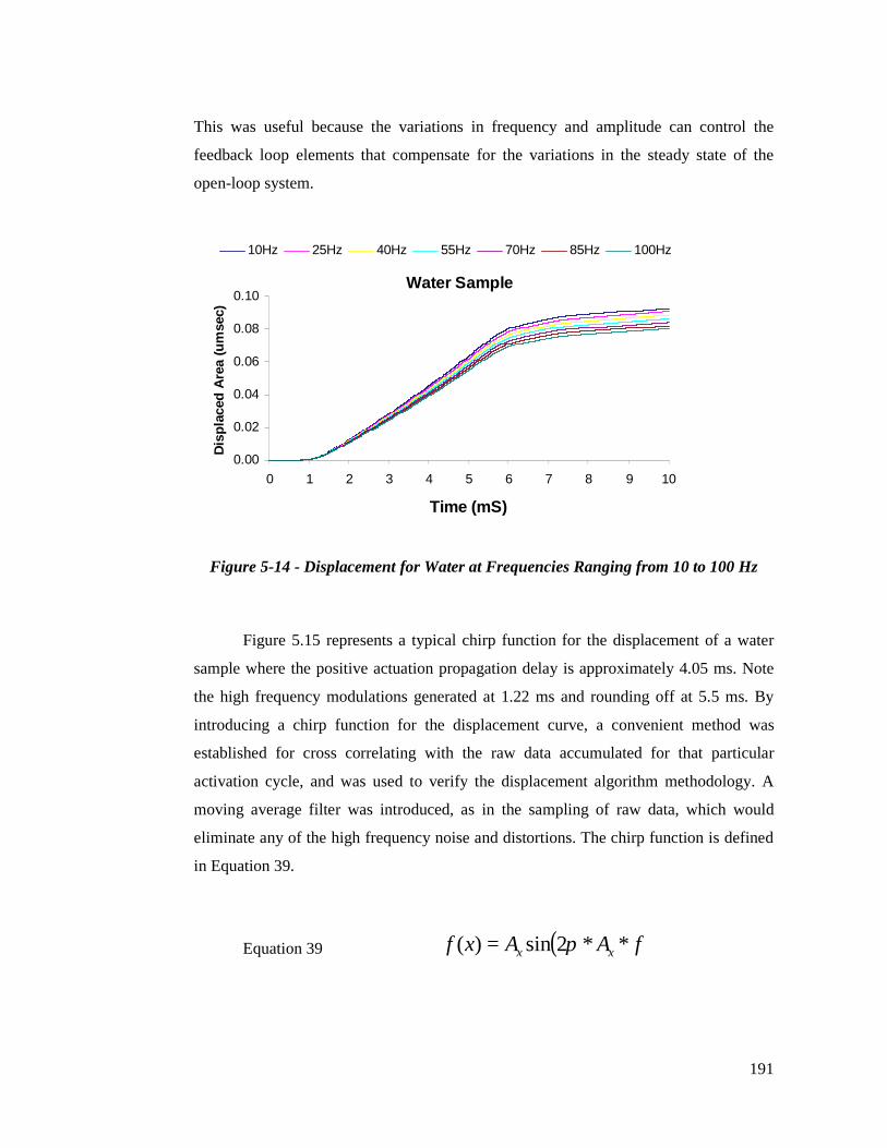
191
This was useful because the variations in frequency and amplitude can control the
feedback loop elements that compensate for the variations in the steady state of the
open-loop system.
Figure 5-14 - Displacement for Water at Frequencies Ranging from 10 to 100 Hz
Figure 5.15 represents a typical chirp function for the displacement of a water
sample where the positive actuation propagation delay is approximately 4.05 ms. Note
the high frequency modulations generated at 1.22 ms and rounding off at 5.5 ms. By
introducing a chirp function for the displacement curve, a convenient method was
established for cross correlating with the raw data accumulated for that particular
activation cycle, and was used to verify the displacement algorithm methodology. A
moving average filter was introduced, as in the sampling of raw data, which would
eliminate any of the high frequency noise and distortions. The chirp function is defined
in Equation 39.
Equation 39 ( )fAAxf xx **2sin)( π=
Water Sample
0.00
0.02
0.04
0.06
0.08
0.10
0 1 2 3 4 5 6 7 8 9 10
Time (mS)
Dis
plac
ed A
rea
(um
sec)
10Hz 25Hz 40Hz 55Hz 70Hz 85Hz 100Hz

192
This function was a means of verification over each individual actuation cycle.
At vibration frequencies ≥ 100 Hz, the latency could present a problem between cycles
as the settling of the actuator diaphragm (Section 34, page 144) could produce a larger
than expected latency.
Figure 5-15 - Area displacement modulation frequency for water
Figure 5.16 is an ideal modulation fringe response based on the actuation pulse
of 5 ms duration during the positive excitation of 400V. It shows normalised unit
amplitude, as generated using Equation 36. Even though the amplitude of the
modulations could vary from pulse to pulse, the correlation between ideal and acquired
samples quantified the differences over frequencies and phases for the response. The
ideal response data served as the basis for measurement of micro-pump reliability and
performance and was used as reference for validating the cycle-to-cycle response data.
Since the steepness of the slopes was proportional to the modulation frequency
of the response, the displacement outcome could be predicted over the entire actuation
pulse as long as the PZT membrane deflection is ideal in its response to the applied
pulse.
Water Sample at 10 Hz
-0.15
-0.10
-0.05
0.00
0.05
0.10
0.15
0 1 2 3 4 5 6 7 8 9 10
Time (mS)
Are
a D
ispl
acem
ent
Enve
lope
(um
2 )
Area Displacement Frequency Displacement

193
Figure 5-16 - Ideal Air Displacement Modulations in a 10 ms Window
Having predetermined the slopes for the ascending and descending displacement
response, it was straightforward to use these as a trigger for starting the data sampling
and processing algorithm.
Figure 5.17 represents the maximum frequency modulations that are sampled,
which limit the bandwidth of the response. It can be seen that at high frequencies the
modulations are greatly attenuated, at which point fall into the area of bandwidth
limitations as indicated in Figure 5.18.
Figure 5-17 - PZT Driver Slew vs Fringes
Ideal Air displacement fringes
0
100
200
300
400
500
0 1 2 3 4 5 6 7 8 9 10
Time (ms)
Act
uato
r driv
er (V
)
-1.5-1-0.500.511.5
Nor
mas
lised
A
mpl
itude
Actuator Ideal modulation frequency
-100
0
100
200
300
400
500
1.5 1.7 1.9 2.1 2.3 2.5Time (mS)
Volt
-50-40-30-20-100102030
mV
Actuator Driver Displacement Modulations

194
Note the attenuated modulations at 2.0 ms, which were due to the amplifier
bandwidth limitations. The steep section of the actuator slope increased the frequency of
the displacement while the amplifier gain bandwidth product of the amplifier attenuated
the photovoltaic signal to a level below the detection for the acquisition sampling
reference. In the case of the closed-loop system, the actuation slope was relaxed to a
slope, which ensured that the bandwidth limitations were not breached. The counting
sequence for each of the fringe cycles was used as the measure for the bandwidth
limitation testing and each of the cycle counts was compared with the preset limit in
order to maintain the actuator slope at the right propagation delay.
Figure 5-18 - Actuator Slope Bandwidth Boundaries
The signal-processing algorithm was applied using hardware high-speed
techniques described in Figure 5.20. The first stage of the process examined the zero-
crossing points that could be shifted according to the trigger requirement. Low pass
filters, prior to buffer storage, removed the drifts associated with the instability due to
temperature and amplifier offsets during real-time operation of the system. The zero
crossing, on a rising edge of the signal, was sampled and minimum and maximum
points were extracted. This was done over the period determined by the PZT driver
rising edge output, which was used as reference for the displacement differential dt.
Time
Am
plitu
de
Bandwidth Boundary
Actuator driver path
Actuator acceptable slope variations
t (mS)
Volt (V)

195
The differentiation of minimum and maximum fringe peaks identified the
frequency at each zero crossing and served as a reference for the displacement counting
technique shown in Figure 5.19.
Figure 5-19 - Fringe Extraction Hardware Algorithm
Figure 5.20 represents a typical fringe extraction and frequency counting timing
diagram to demonstrate the process employed for displacement measurement. The
trigger section was referenced to the PZT driver actuator pulse and also to the frequency
and amplitude of the waveform generated during the application of the PZT actuator.
Figure 5-20 - Typical Fringe Extraction Timing Representation (Generated running
the waveform simulation for the circuit of Figure 5.19)

196
For the purpose of calibration and verification of the electronics described in the
methods section, the initial tests were performed using a piezoelectric buzzer (audio
transducer), driven by a sine wave of varying frequency.
By differentiating across the generated fringes and extrapolating the maximum
and minimum points (Figure 5.21) it was possible to plot the rate of increase dV with
respect to t, where dV/dt is the differential coefficient of amplitude V with respect to t.
The turning points were determined using the dV/dt = 0 = tan θ, and the subsequent
frequency interpolated from the distribution of minimum and maximum peaks.
Figure 5-21 - Sum of Differentials |dv/dt|
The displacement of the diaphragm was measured by the number of fringes
multiplied by the wavelength of the source (Figure 5.22).
Displacement differential
-505
10152025303540
0 0.45 0.9 1.35 1.8 2.25 2.7 3.15 3.6 4.05 4.5
time (ms)
Sum
of D
iffer
entia
l (dy
) V

197
Figure 5-22 - Audio Tweeter Displacement Based on 632.8 nm Modulation Fringes
During the positive transition of the applied PZT potential, a sudden change in
frequency was used as a trigger point for the initialisation of the displacement signal-
processing (DSP) algorithm. The DSP algorithm was averaged over a number of
samples to filter out the high frequency noise modulated by the fringe coefficients. This
was an adaptive function, calibrated during the manufacturing process, which can vary
within a predetermined parameterised coefficients range (FIR filter taps).
5.5 PZT Driver Closed-loop Feedback Analysis
Open-loop experiments showed that the amplitude of the PZT driver varied with
the type of medium being processed. The reduction in the PZT driver amplitude, due to
the medium being processed, indicated that the mechanical loading affected the PZT
driver circuit. In order to correct this, by a way of compensation, a set of feedback loop
coefficients was generated and saved as lookup tables in the non-volatile memory of the
system.
PZT Tweeter Displacement
0.01.02.03.04.05.06.07.08.0
0 0.45 0.9 1.35 1.8 2.25 2.7 3.15 3.6 4.05 4.5
time(ms)
disp
lace
men
t (um
)displacement

198
Water was used as the medium to reference the micro-pump parameter
variations for the PZT driver. A number of outcomes were plotted showing the effect of
varying the frequency, amplitude and phase for the PZT driver based on the percentage
variations adjusted using the feedback closed-loop system configuration.
Figure 5.24 shows the percentage variation at each sample point for water
stimulated with 10 Hz at full 400V PZT amplitude drive. The coefficients were
determined by applying the algorithm of Figure 5.23. Effectively, the percentage
algorithm illustrates the amount of change relative to the overall average displacement
variation for the 60s duration, sampled at 10s interval.
Figure 5-23 - 10 Hz Water Displacement Coefficient Generating % Variation
Algorithm
START
MIN = 0
MAX = 0
No
Yes
Yes
No
100*minmax
avnnn −
N %

199
Figure 5.24 illustrates the percentage variation based on the algorithm of Figure
5.23. This was useful in determining the overall change during each of the cycle
spreads for the displacement of the actuator membrane. By considering a percentage
variation, it was possible to determine the critical paths over the variable dv/dt
considered as the maximum displacement area derivative shown in Figure 5.25. Note
that the initial non-triggered area of Figure 5.24 indicated no displacement variation for
which the period is shown in Figure 5.16 as the intermediate frequency diaphragm off
state.
As illustrated in Figure 5.24, maximum variation occurred during the trigger
event that established the sampling beginning for the cycle. This could be attributed to
the initial start-up detection pulse that could be either negative or positive in its phase
position, depending on the quadrature component at which it had entered the start-up
phase. Note that in the period between the 1st and 6th milliseconds of signal processing,
the variations were at their minimum, which was attributable to the low frequency
modulation rates that were exhibited over that period.
Figure 5-24 - 10Hz Water Displacement % Variation from which the PZT Driver
Coefficients were Generated
10Hz Water Displacement % Variations
012345678
0 1 2 3 4 5 6 7 8 9 10
Time (ms)
% D
ispl
acem
ent
Var
iatio
n
% variations

200
Figure 5.25 shows the maximum effective displacement variation between each
of the samples for the 60s window spread, segmented in 10s intervals. It is this variation
spread that is used to determine the overall variation displacement for the 60s sampling
window. In this case, it can be seen that the spread is very evenly spread across the
10ms. If each sample is taken for the variation comparison during feedback, the closed-
loop coefficient determination may not be accurate since the calculation does not allow
for the individual sample calculation. It is intended as the moving average calculation,
considering a spread of 10 samples, as indicated in Figure 5.26.
Figure 5-25 - Maximum Water Displacement Variations for 10Hz Excitation
Frequency
By applying the feedback moving average filter of Equation 26 to the
displacement data, the response in Figure 5.26 shows the effect of the feedback when
the algorithm in Figure 5.23 is executed.
Maximum 10Hz Water Displacement Variations
0.0E+005.0E-031.0E-021.5E-022.0E-022.5E-023.0E-023.5E-02
0 1 2 3 4 5 6 7 8 9 10
Time (ms)
Dis
plac
emen
t (um
)
Maximum Displacement Variation

201
Figure 5-26 - Moving Average Feedback Response (10 samples)
Note the reduction in the spread, which was attributed to the averaging feedback
loop. The samples taken were that of water at 10 Hz excitation frequency and 400 V
excitation amplitude.
The contents of Table 5.3 show the effects of varying the PZT driver amplitude.
The displacement of the actuator diaphragm dropped with a decrease in the PZT driver
amplitude, as expected. The same applied to the flow rate of the fluid or liquid flowing
through the micro-pump chambers.
PZT Driver Amplitude (% variation) Water
sampled at
10Hz 100 98 96 94 92 90 88
Amplitude
(V) 400 392 385 377 368 361 352
Displacement (um) 19.23 18.87 18.49 18.10 17.72 17.34 16.95
Flow Rate (ul/min) 81.21 79.70 78.09 76.45 74.85 73.24 71.60
Table 5.3 - 10Hz PZT Driver Amplitude Variation Effect for Water
10 Sample Moving Average Feedback response
0.0E+00
5.0E-03
1.0E-02
1.5E-02
2.0E-02
2.5E-02
3.0E-02
0
Time (ms)
Dis
plac
emen
t (um
)
Maximum Average Displacement Variation

202
This was useful in determining the feedback coefficients for the PZT driver
amplitude, which directly altered the response of the system (Figure 5.27).
Figure 5.27 shows the relationship between the PZT driver variations as applied
using the feedback coefficients generated from the characterised open-loop response
described in Chapter 4. Note the linearity of the response with flow rate as well as the
proportionality to the displacement plotted in Figure 5.28. This shows that the linearity
is uniform for all three parameters and can therefore be applied to the feedback transfer
functions described in Section 4.10. Any value up to 12% variation in the PZT driver
amplitude linearly affected the actuator membrane sufficiently to have the effect of
compensating for the error variations of the system.
Figure 5-27 - PZT Driver Variation from 1 – 12% and its Effect on Flow Rate for
Water at 10Hz Excitation
The same effect was observed for frequencies up to 100Hz. Figure 5.28 shows
the linearity between the flow rate and the displacement of the actuator membrane. The
samples were taken over a 60s interval for each of the percentage variations.
PZT Driver Amplitude for 10Hz excitation
340350360370380390400410
889092949698100
PZT % variation (%)
Am
plitu
de (V
)70.00
72.00
74.00
76.00
78.00
80.00
82.00
Flow
Rat
e (u
l/min
)
PZT Driver Flow Rate

203
Figure 5-28 - PZT Driver Variation from 1 – 12% and its Effect on Displacement and
Flow Rate for Water at 10Hz Excitation
Table 5.4 shows data accumulated during sampling of air 60 seconds at varying
frequencies. Note the uniformity between the variations, 3.34% maximum between
frequencies from 10 Hz to 100 Hz. The maximum displacement variation is 13.64% and
the flow rate of air was not measured during these experiments. The maximum
variation in the displacement was observed for air as shown in Figure 5.29, and the
minimum variations occurred at 25 Hz and 85 Hz taken over a sample point variations
during a 10 ms interval.
Figure 5-29 - Maximum Variation for Air Using Feedback Loop
PZT Driver Amplitude for 10Hz excitation
70.00
72.00
74.00
76.00
78.00
80.00
82.00
889092949698100
PZT % variation (%)
Flow
Rat
e (u
l/min
)
16.50
17.00
17.50
18.00
18.50
19.00
19.50
Dis
plac
emen
t (u
m)
Flow Rate Displacement
Maximum point to point variations (AIR)
0.0565
0.0570
0.0575
0.0580
0.0585
0.0590
0 20 40 60 80 100 120
Frequency (Hz)
Disp
lace
men
t (um
)
Sample variation

204
Table 5.4 - Closed-loop Response for Frequencies Ranging from 10 Hz to 100 Hz
and Four Pumping Media (air, water, water+28% and 60% glycerol)
The linearity of the flow rate indicates that the point-to-point variations did not
introduce any significant changes (Figure 5.30).
If we consider the plot for all media combined over a range of frequencies, air
fluctuated with a greater degree of variations between frequencies (Figure 5.31). This
may be attributable to under-dampening of the actuator diaphragm.
Medium Tested
Frequency Hz
CL MAX Total
Variation
CL MAX
% Variation
CL AVERAGE
Total Variation
CL AVERAGE
% Variation
CL MAX Disp. (um)
CL Flow Rate
(ul/min)
10 0.0583 7.02 0.03004 0.57 28.9125 0.0567 7.68 0.03009 0.59 28.2440 0.0575 8.82 0.03004 0.60 27.5755 0.0586 8.21 0.02989 0.61 26.8970 0.0585 8.90 0.03005 0.63 26.2385 0.0566 9.23 0.03000 0.64 25.59
100 0.0580 10.21 0.02998 0.66 24.9610 0.0319 6.79 0.01705 0.49 19.23 82.1625 0.0330 7.03 0.01697 0.50 18.78 200.6540 0.0325 8.06 0.01706 0.51 18.34 313.4155 0.0324 7.37 0.01699 0.52 17.89 420.4570 0.0328 8.46 0.01708 0.54 17.44 521.7885 0.0319 8.11 0.01704 0.55 17.02 618.15
100 0.0333 8.10 0.01712 0.56 16.61 709.5710 0.0194 5.21 0.01005 0.35 15.83 67.6225 0.0192 4.55 0.00997 0.35 15.46 165.1440 0.0189 5.15 0.00998 0.36 15.09 257.9655 0.0188 5.14 0.01006 0.37 14.72 346.0470 0.0189 5.00 0.01001 0.38 14.36 429.4585 0.0194 5.33 0.01001 0.39 14.01 508.69
100 0.0193 5.49 0.01002 0.40 13.67 584.0310 0.0096 3.60 0.00501 0.26 10.45 44.6425 0.0094 3.60 0.00502 0.27 10.21 109.0140 0.0096 4.08 0.00502 0.27 9.96 170.2855 0.0095 3.76 0.00500 0.28 9.72 228.4470 0.0095 3.83 0.00501 0.28 9.48 283.4885 0.0095 4.23 0.00501 0.29 9.25 335.87
100 0.0095 4.25 0.00499 0.30 9.02 385.50
AIR
WATER
GLYC28%
CLYC60%

205
Figure 5-30 - Flow Rate for Water using the Feedback Loop
Figure 5-31 - Maximum Displacement Variation for Each Sample Point and Range
of Frequencies
Figure 5.32 shows the displacement variation between media sampled at
frequencies ranging from 10 Hz to 100 Hz. The drop, as frequency increased, was
caused by the PZT loading (electrical load), which occurred as the viscosity of the
medium decreased. The rate of change across all of the tested media was linear and
constant, and the drop in displacement was directly related to the latency of the actuator
Flow Rate vs. Frequency
0.00100.00200.00300.00400.00500.00600.00700.00800.00
0 20 40 60 80 100 120
Frequency (Hz)
Flow
Rat
e (u
l/min
)
Flow Rate
Maximum sample variations
0.000.010.020.030.040.050.060.07
10 25 40 55 70 85 100
Frequency (Hz)
Am
plitu
de (u
m)
AIR WATER GLYC28% GLYC60%

206
movement due to the load viscosity variations. This was indicated by the lower than
usual frequency of the extracted fringes. The greater the rate of change for the
displacement, the greater the frequency of the interferometric fringes.
Figure 5-32 - Maximum Displacement Closed-loop Response Variations
Flow rate is measured only for water; water with 28% glycerol, and water with 60%
glycerol (Figure 5.33).
Figure 5-33 - Closed-loop Flow Rate Analysis Using Three Media (water, water+28%
and 60% glycerol)
Maximum Displacement
0.005.00
10.0015.0020.0025.0030.0035.00
10 25 40 55 70 85 100
Frequency (Hz)
Dis
plac
emen
t (um
)
AIR WATER GLYC28% GLYC60%
Flow Rate Analysis
0100200300400500600700800
10 25 40 55 70 85 100
Frequency (Hz)
Flow
Rat
e (u
l/min
)
WATER GLYC28% GLYC60%

207
6 Open and Closed-loop Comparison Analysis

208
6.1 Open-loop / Closed-loop Comparison Analysis
In Section 5.4, we looked at the results based on a closed-loop configuration as
described in Figure 4.12, without comparisons to the open-loop results of the previous
chapter. This section compares the results from the open-loop results with the closed-
loop data.
The open-loop Table 5.2 and closed-loop Table 5.4 contain the data for “MAX
Total Variation”, where each sampled point n was compared with the last sampled point,
at each of the 10 seconds intervals, over the duration of 60 seconds. The difference was
saved and at the end of the sampling period (60s), the difference between maximum and
minimum points was calculated, giving a total variation for that sample point, nmax –
nmin.
The maximum total variation refers to the total sample, spread over 10,000
points (N), where maximum point variation P∆max = (nmax – nmin)*N (refer to file
“OL_water_disp_10Hz_60s” in the PhD Lab directory). The maximum total variation is
a numerical value of the displacement (µm) for each sampled point over the 10 ms
window, captured every 10 seconds for the duration of 60 seconds. The pulse of
excitation (stimulus) was 5 ms in duration and the rest of the 10 ms cycle was taken up
with the initialisation trigger starting latency, and the decaying settling period between
cycles. The maximum variations are represented as units of displacement µm and also as
the percentages of the total. In addition, the average total variation and its percentage
representation are also included in the evaluation, which allows for a more accurate data
comparison without inclusion of individual segmented data files. The data files are
represented in Excel spread sheet format, imported from the text files captured directly
from the micro-pump characterization and analysis platform of Figure 3.42.
Table 5.3 shows an increase in point-to-point variations in the displacement,
when the closed-loop is removed, which is directly attributable to the removal of the
input FIR filter and the moving average filter expressed in Equation 26. The average
difference between the open-loop and closed-loop is shown in Table 6.1, where the

209
average rate of change between media was 1.35*m-1, where m-1 is the preceding
medium.
Table 6.1 - Average Difference Between Open and Closed-loop Data for the
Displacement of Differing Media
The average percentage variation shows the changes for the full sample spread,
where the maximum variations occurred during the high frequency excursions. Since
each sample point was compared with the previous sample point, and the phase
alignment between samples was not synchronised, large variations were possible, as
shown in Figure 6.1. Averaging corrected for the phase misalignment and allowed for
generation of coefficients that were applied in the transfer functions for the closed-loop
system.
Figure 6.2 illustrates the difference between the open and closed-loop variations
and, notably, the closed-loop variations were reduced by an average of 39% across the
whole of the 10 ms frame. Similarly, up to 68% reduction was achieved for 60%
glycerol solution (Figure 6.3).
If the variations were less than the minimum resolution for the PZT driver (0.5%
of the maximum potential), the closed-loop transfer function was not activated (Table
5.3).
AIRWATER28%Glyc60%Glyc
Average difference %27.8739.2752.8668.81

210
Figure 6-1 - Percentage Variation for the Displacement Plotted for Open and Closed-
loop Data Sampled for 60 seconds at 10 Hz.
Figure 6-2 - Plot of Point-to-Point Displacement Variation for the Open-loop and
Closed-loop Comparison extracted from Tables 5.2 and 5.4
OL-CL Water at 10Hz percentage variation
0
2
4
6
8
10
12
0 1 2 3 4 5 6 7 8 9 10
Time (ms)
Dis
plac
emen
t (%
um
)OL % variations CL % variations
High frequency up slope
Low frequency max slope
High frequency down slope
Open-loop / Closed-loop Variation Analysis
0.000.010.020.030.040.050.060.070.080.09
OL
Var.
CL
Var.
OL
Var.
CL
Var.
OL
Var.
CL
Var.
OL
Var.
CL
Var.
Disp
lace
men
t Var
iatio
n (u
m)
10Hz 25Hz 40Hz 55Hz 70Hz 85Hz 100Hz
AirWater
Glyc28%
Glyc60%

211
By applying Equation 34 and 35, the area of the displacement was mapped for
each of the frequencies and the media. Since the frequency also varied the displacement,
a variation of less than 0.5% could be achieved - experimentally it was reduced to less
than 0.18%. Unless there was a large fluctuation in the displacement whilst pumping
any of the four media, the closed-loop functionality was reduced to filtering and
averaging of the sampled cycle data. Table 6.2 shows that the overall effect on the flow
rate was negligible between the open and closed-loop performance.
Table 6.2 - Flow Rate Comparison Between Open and Closed-loop System Based on
the data of Tables 5.2 and 5.4
The average percentage variation for the open-loop response is used as a
reference in determining the trigger for initiating the feedback transfer function. The
transfer function was based on the proportional integral control algorithm, and Figure
6.3 shows the response of the system when the algorithm was executed.
OL Flow rate
CL Flow rate
OL Flow rate
CL Flow rate
OL Flow rate
CL Flow rate
82.19 82.16 67.67 67.62 44.68 44.64200.97 200.65 165.29 165.14 109.17 109.01314.03 313.41 258.18 257.96 170.35 170.28420.90 420.45 346.37 346.04 228.68 228.44522.37 521.78 429.83 429.45 283.86 283.48619.14 618.15 509.19 508.69 336.31 335.87710.78 709.57 584.46 584.03 385.96 385.50
WATER GLYC28% GLYC60%

212
Figure 6-3 - Trigger Window for Closed-loop Operation Initialisation
The closed-loop percentage variation was reduced by up to 60% for water over
the entire frequency spectrum, while the point-to-point variations were reduced
proportionally within the confines of the percentage error window area (Figure 6.3).
Table 6.3 shows the comparison data between media for the percentage sample
variations. A significant improvement was observed for water with 60% glycerol
added. The error variation was reduced by 3.15% across all of the frequencies, which
can be also related to displacement variation data plotted in Figure 6.2.
Table 6.3 - Open and Closed-loop Average Percentage Variation Comparison Table
Average % Variation for water
0.00
0.20
0.40
0.60
0.80
1.00
10 25 40 55 70 85 100
Frequency (Hz)
Aver
age
Varia
tion
%
Open Loop Closed Loop
% Error window
OL %
Average
CL %
Average
OL %
Average
CL %
Average
OL %
Average
CL %
Average
OL %
Average
CL %
Average10 0.79 0.57 0.81 0.49 0.72 0.35 0.82 0.2625 0.81 0.59 0.82 0.50 0.73 0.35 0.85 0.2740 0.83 0.60 0.84 0.51 0.76 0.36 0.87 0.2755 0.85 0.61 0.87 0.52 0.78 0.37 0.90 0.2870 0.87 0.63 0.88 0.54 0.80 0.38 0.91 0.2885 0.89 0.64 0.91 0.55 0.81 0.39 0.93 0.29100 0.90 0.66 0.93 0.56 0.83 0.40 0.96 0.30
GLYC60%
Freq. Hz
AIR WATER GLYC28%

213
6.2 Comparison Summary
Using the laboratory-on-a-board system, outlined in Figure 3.42, as the platform
for closed-loop testing and analysis, it was necessary to establish a correlation between
the results obtained in the open-loop experimentation, using a discrete hardware
platform (described in Chapter 3). This was achieved by repeating the original open-
loop experiments and then calibrating the optical and front-end analog interface on the
new and fully integrated (laboratory-on-a-board) platform of Figure 3.42.
The software processing algorithms on the laboratory-on-a-board were identical
to the discrete hardware used earlier because the FPGA signal processing hardware was
also kept the same. The major departure in the platform of Figure 3.42 was in the
addition of a closed-loop hardware section (also implemented in the FPGA). From a
control perspective, this drove the step-up transformer and phase shaping circuitry was
also added
The project outcome for the closed-loop analysis showed some interesting and
unexpected results, especially with reference to flow rate and the displacement
variations.
The flow rate difference between the open and closed-loop results was
negligible, as indicated in Table 6.2, and similarly for the displacement, as indicated by
the data in Tables 5.2 and 5.4. This can be attributed to low cyclic variations exhibited
during the open-loop sampling, since the closed-loop was only invoked when the area of
the overall cycle displacement was either increased or decreased by the amount that
triggered the feedback transfer function algorithm (Figure 6.3). The sampling frame of
60 seconds was not sufficient to accumulate the percentage error variations required to
trigger the closed-loop transfer function. When triggered, the frequency or amplitude
coefficients were invoked by the controlling transfer function.

214
6.3 Integration Issues
Based on the open and closed-loop experimental analyses, it was fitting that a
suitable integration technique, for combining the mechanical, electrical and optical
systems into a single package, was considered. The package would need to include:
• A micro-electro-mechanical-system (MEMS) micro-pump driven by a
piezoelectric element bonded to a flexible diaphragm
• An interferometric sensor fabricated using polymer optics
• Microelectronics for analysis and control.
The package concept was compatible with the Field Programmable Gate Array
(FPGA) technology, which also allowed for the integration of low cost, high
performance polymer optic components. Typical devices that could be heterogeneously
integrated on a standard FPGA Flip-Chip Pin Grid Array substrate and bonded over the
polycarbonate layers included:
• Pin photo-detectors
• Pin laser diodes
• Polymer waveguide arrays
• Collimating/focusing lenses
• Directional couplers (splitters)
• Piezoelectric drivers.
These could constitute a closed-loop MEMS micro-pump.
The main advantage of this type of approach to integration include:
• Optical ports alleviating distance limitations
• Reduction of noise and ambient interference

215
• Elimination of the need for drift compensation
• Facilitation of self calibration and performance monitoring.
This type of integration would be well suited to applications with medical and chemical
diagnostic devices.
Figure 6.4 illustrates a single silicon wafer as it is configured for integration of
polymer optic waveguides with polymer based components. Polymers are chosen for
the integration platform because of their low-cost and ease of manipulation with
standard methods such as stamping, embossing, wet and dry etching and can be worked
at room temperature. In the past polymers were considered to incur high propagation
losses across their planar waveguides compared with silica. Additionally, the thermal
characteristic guarantee a higher thermo-optic coefficient, than for silica, which leads to
greater power efficiency. The polymers would need to be high-technology polymers
because they require rapid processing and would need to be cost-effective while
offering high yields. They exhibit a large refractive index that translates into greater
integration based on highly compact components.
Figure 6-4 - Polymer Optics Planar Wave-guide Channelling
The most common classes of polymers used for integration on Silicon substrate
base include polycarbonates, polyimides, olefins and acrylites. Processing of these
Return channel interconnect
Laser diode doping
Polymer wave-guides
Collimating and focusing polymer
Silicon Substrate

216
polymers may very, depending on their characteristics. For example, polycarbonates
can only be processed using reactive ion etching since they are not photosensitive.
Being highly transparent, optic polymers generally have loss values of less than
0.1 dB/cm at wavelengths from 840 nm to 1550 nm. Direct photo-patterning in
polymer waveguides minimises scattering losses and direct polymer lithography can
also be used to minimise the roughness caused by the processing technique by a way of
interlayer diffusion. Another advantage polymer optics exhibit over silica structures is
in their ability to be designed to form stress-free layers independent of the substrate
composition, which is usually free of the stress induced scattering loss and polarization
dependence.
The polymer integration component types that were being considered at the time
of writing this thesis were in the areas of attenuators, filters, lasers, amplifiers, switches,
modulators, collimating and focusing lenses, directional couplers, mirrors and prisms.
In the case of the interferometer required for micro-pump feedback, all of the
components could readily be constructed from polymer based materials of any of the
previously mentioned classes.
A current technique for producing lasers and optical amplifiers (i.e., rare-earth
doping) proved to be reliable, low-cost and had a wide gain bandwidth, but was mainly
used in silica. Rare-earth doping was being investigated for polymers, but at the time of
compiling this dissertation, was still proving to be unstable due to the de-excitation of
the excited states, caused by the IR absorption in the polymer. A breakthrough had to be
made in the use of low IR absorption, high-stability polymers in order to make this
technology viable.
The laser and amplifier could be fabricated by inserting indium phosphide (InP)
and gallium arsenide (GaAs) laser integrated circuits that could generate or amplify
light or convert wavelengths such as modulation fringes, as in case of the Mach-
Zehnder interferometer used for our experimentation.

217
Integration of the micro-pump, electronics and polymer optics could be achieved
on layers of silica wafers, even though some of the processes may involve differing
techniques. This could be achieved through parallel processing and machining before
integration. Figure 6.5 is the representation of a cross-section for a fully integrated
intelligent micro-pump and electronic control system (with components described in
Table 6.4).
Figure 6-5 - Cross Section of a Fully Integrated System
Item Description Item Description Item Description
1 Power Inverter 13 Thermal analog I/F 25 Micro-pump polycarbonate layer 1
2 Pulse coil 14 Inductive analog I/F 26 Micro-pump polycarbonate layer 2
3 Pulse shaper 15 ADC filter 27 Polymer lens chamber
4 Phase controller 16 Directional coupler substrate 28 Valve lever membranes
5 Amplitude controller 17 Diaphragm cavity + depressurization valve 29 PZT copper terminals
6 FPGA dye 18 Thermal sensor 30 Inlet
7 Hybrid polycarbonate enclosure 19 Outlet 31 Polymer phase shifter
8 Trans-conductance amplifier 20 Micro-pump
embodiment 32 Laser modulator
9 FIR filter 21 Flow Rate sensor 33 Laser diode doping
10 Photodiode doping 22 PZT membrane 34 Dielectric barrier
11 Analog isolation barrier + AD converter 23 Metal diaphragm 35 Polymer tunable grating
12 IR transceiver 24 Main chamber 36 Metal interconnect layer
Table 6.4 - Integrated System Block Descriptions
2
1 7 3 4
5 6
8 9 11 12
15 14 13
32 33
34
31
30
29
28 26 25
24 23
22
16
21
27
20
17
10
19
18
35

218
7 Conclusions and Recommendations

219
7.1 Overview
Design and test techniques were applied to a micro-pump with the objective of
identifying and parameterising the steady-state dynamic variables during the
displacement measurement of the piezoelectric actuator, using a fibre optic
interferometer. The parameterised evoked potentials (elicited by the fibre optic
interferometer) were accumulated and processed, identifying control elements that could
be applied in an adaptive closed-loop environment. It was shown that the displacement
of the piezoelectric actuator was dependant on the:
• Pumping medium viscosity and density
• Peak PZT driving voltage, its rate of change and frequency actuation.
Fully functional and experimentally optimised electronic modules were developed,
incorporating high bandwidth photo-detector amplifiers, high speed analog to digital
converters, a digital signal processing unit and a high voltage inverter for feedback-
control of the piezoelectric membrane actuator.
It was possible for the entire digital signal processing elements to be implemented
in a single complex programmable logic device (CPLD). This would allow for dynamic
re-programmability implementation on demand, beneficial for applications requiring
control logic (functional) changes without having to modify the physical layout or
structure of the system. It was also demonstrated that it was possible to produce an
adaptive closed-loop system model based on the characterization of a micro-pump using
a fibre optic interferometer. Comparisons were performed between open- and closed-
loop performance.

220
7.1 Specific Contributions
This Doctoral research program is perceived to have made some specific
contributions to the field of micro-systems research. Specifically:
(i) A comprehensive literature review was completed and documented in the
field of micro-pumps and their performance evaluation. The literature
review provided access to a body of work from learned peers that
contributed to the specific research directions herein.
(ii) A discrete-component electronic test system was designed and implemented
for the purposes of characterising the open-loop behaviour of a micro-pump.
A complete discrete component test platform was designed and developed
and used to precisely and accurately characterise the open-loop response of
a micro-pump (Figure 3.9 and Figure 3.21). In addition to the hardware
development, all of the functions were also software generated, which
replaced a conventional PC based analysis platform that could only handle a
sample at a time. The platform brought together a fibre optic interferometer
interface, all associated electronics that converted optical information into
electrical pulses while simultaneously accumulating and analysing the
results in real-time operation. Immediately, it become possible to view and
analyse multiple samples simultaneously, which eliminated the need for
frame-by-frame processing. Since the hardware was implemented in a
dynamically configurable FPGA, variation in the micro-pump
characteristics was readily accommodated. The fine-tuning of the fringe
extraction algorithms was simply a matter of macro selection and could be
readily changed. The calibrations and verifications were performed with a
counter lever laser technique using a commercially available precision
instrument.

221
(iii) Based on experimental findings relating to the micro-pump, and
performance evaluation of the discrete component test system, a more
sophisticated laboratory-on-a-board test system was developed to provide
closed-loop control and testing facilities. The closed-loop control
experimentation required a test platform that could also drive the PZT
actuator of the micro-pump while monitoring the interferometer modulation
fringes. In addition, the platform needed to control the PZT driver in real
time and in a closed-loop configuration while communicating with an
external PC platform for visual monitoring. This led to the design and
development of the laboratory-on-a-board experimental test platform as
shown in Figure 3.42
(iv) This platform incorporated complete electronics required for the closed-loop
operation and analysis of a micro-pump. New software macros and
mathematical algorithm for the transfer functions were generated and a
complete set of open-loop data was regenerated. The regeneration of the
open-loop data was needed to bring the results in line with the new micro-
pump being tested.
(v) Flow rate analysis was performed, between open and closed-loop
operations, and both quantitative results and qualitative observations were
documented
(vi) The process of developing an integrated “system on a chip” process for the
purposes of a commercial application, based upon the closed-loop
interferometric approach, was investigated and documented.
(vii) The results of the experimentation were published in the Proceedings of
SPIE in 2002.

222
7.2 Enveloping Broad-Context Discussion
7.2.1 Characterisation and Open-Loop Performance
Documented research in the area of free-running, open-loop, piezoelectrically-
driven micro-pumps (Chapter 2), covered, in some detail the structural, mechanical and
electrical aspects of such systems. Through an analysis of each of the disciplines
covered within the literature review, it became obvious that a number of areas were of
concern with respect to performance reliability and implementation. This also became
evident during the first three months of preliminary experimentation with a number of
commercially available micro-pumps that were used in this Doctoral research. In one
instance, a micro-pump lasted for less than two hours of continuous operation before
complete structural failure while pumping water. Another simply failed when the inlet
valve clogged when 28% of glycerol was added – even though the documented
procedures relating to viscosity of media were applied.
The micro-pump failures seemingly occurred without warning, and the first
physical indication of impeding failure was when the flow rate was reduced to zero. The
PZT driver continued to pulse the actuator membrane at the pre-selected frequency,
phase and amplitude, until the internal chamber pressure increased to a level that finally
broke through the polycarbonate bonding. Upon further investigation, one of the micro-
pump failures was captured during sampling while displacement was being
characterised. This revealed that the failure was, in fact, progressive and slow, as
indicated by the analysis of the sampled responses. The first indication was a drop in the
PZT driver amplitude (noted when an oscilloscope was used to monitor the PZT driver
output) and the modulation frequency.
The open-loop experimentation platform that was developed for the
characterisation phase of this Doctoral research was composed of a number of discrete
elements, such as a central processing unit; analog data acquisition module, and a
commercially available piezoelectric driver unit (specific to a particular type of micro-
pump manufacturer). For this reason, a number of system monitoring instruments had

223
to be attached for the purpose of calibration and verification of the system during
operation. This was beneficial since it was not possible to continuously sample and store
each of the cycles, and a staggered sampling was implemented. It became evident,
relatively quickly when observing the cycle-to-cycle data, that the variation of the
displacement fluctuated significantly when structural or mechanical failures were about
to occur. This was subsequently further investigated by using a faulty micro-pump,
where a pressure leak (due to the ungluing of the PZT membrane normally firmly
attached to the metal diaphragm) was detected. The pump continued to work for some
time, but with unacceptable rates of fluctuations between cycles, which was also
reflected by the flow rate measurement data.
Normally, a free running micro-pump was expected to exhibit a stable and
consistent response over its resonant frequency and, under normal circumstances, this
was the case. However, it was observed during the preliminary experimentation that,
without the external monitoring of flow rate for a given pumping medium, unreliable
delivery could arise. Clearly, in instances where accurate drug or chemical solution
delivery was important, this was not acceptable, and it was for this reason that the
Doctoral research program sought to investigate the efficacy of a closed-loop system
option.
During the open-loop characterisation, it was determined that the steady state
response of the system was influenced by a number of parameters, such as frequency,
amplitude and the pumping media itself. It was also noted that normalised responses
might be mapped for each of the media, which would be consistent over the specified
values. The implication for such a system, where each characterization was performance
mapped, could be of great benefit in applications where accurate drug or chemical
delivery systems were considered important.
Through the experimentation documented in Chapter 4, it was evident that the
open-loop response of a micro-pump, mapped and characterised with a reliable non-
contact fibre optic interferometer, and in conjunction with a reliable experimentation

224
platform, yielded valuable information, which aided in the design and development of a
reliable closed-loop system.
7.2.2 Closed-Loop Performance
The open-loop investigation identified a number of reasons why a closed-loop
system could be beneficial in applications where a stable and reliable drug or chemical
delivery was required. These included:
• Impurities in the pumping medium, causing fluctuations in the actuator
displacement.
• Temperature variation between the input and output valves and the main
chamber.
• Sudden changes in chamber pressure due to air bubbles
• Progressive cyclic loss of pressure due to structural and mechanical failures
• Drop in the piezoelectric driver amplitude due to a faulty pulse generation
magnetics or electronics.
This open-loop investigation was undertaken with a discrete component testing
system developed for this Doctoral research. However, it became apparent during
testing that, for the purposes of closed-loop control, a more sophisticated experimental
laboratory would need to be designed and constructed. This resulted in the laboratory-
on-a-board system as shown in Figure 3.42. This represented a significant research and
development exercise in its own right. A further enhancement, incorporated into the
laboratory-on-a-board system, was that the signal processing algorithm was
implemented in hardware, which needed to be independent of the software processing
algorithm because of the high speed sampling rate required to capture high bandwidth
modulations sampled by the fibre optic interferometer trans-conductance amplifier.
The development of the more sophisticated laboratory-on-a-board platform
provided a useful mechanism for verification of the open-loop analysis originally

225
performed with the discrete component system. An examination of the two sets of data
showed some variation between the two sets of data, but the results proved to be
consistent, given that a different brand of micro-pump (with similar characteristics) was
used during the verification experiments (as a result of a lack of availability of the
original brand). The behavioural analysis of Section 5.4 showed a greater frequency
spread and its relationship to actuator displacement. In addition, a complete
piezoelectric driver characterization was also mapped, indicating a relationship between
amplitude and displacement.
In terms of closed-loop control, the comparison analysis of Section 5.5, showed
that if variations for the actuator displacement were below a minimum level, over a
predetermined sampling period (60 seconds), the closed-loop transfer functions were
not triggered, with the exception of the filter and averaging functions. These functions
then had the effect of improving the percentage error variations over a complete cycle,
evaluated on a per sample basis. In the case of short duration sampling, the flow rate
variations were negligible, and the closed-loop data, accumulated and averaged,
maintained a steady state performance reference, and in turn acted primarily as a failure
predictability function.
Any sudden variations in the actuator displacement (above the trigger threshold),
over the predetermined period, invoked the forward error correction transfer function
documented in Section 4.9. The overall effect caused a single cycle correction algorithm
that could use amplitude or frequency as the adaptive function, depending on the
window of rate of change with which the data was correlated.
The analysis of the closed-loop data showed that the performance and reliability
of an open-loop system, pumping homogeneous media, would improve only marginally
over a short period of time. This marginal variation was due to a very short sampling
period which, if extended, became more effective in maintaining consistency over the
flow rate control.

226
The electronics that maintained equilibrium for the closed-loop system could be
integrated onto a number of silica wafer layers that could also incorporate polymer
optics and the micro-pump structure. These could then be combined to form a single
hybrid block (Figure 6.4). In the context of this Doctoral research, however, only a
hypothetical model was considered, based on the research outlined in Section 2.5.4.
7.2.3 Summary Comparison Between Open-Loop and Closed-Loop Control
By evaluation of the open-loop analysis, it can be seen that the variations in the
cycle to cycle-performance (for homogeneous pumping media) were small, and only
became significant with:
• Changes in the viscosity of the medium
• Detection of crystallisation or granulation due to contamination
• Slow degenerative structural failures.
For this reason, in the case of low-risk pumping activities, particularly when
using homogeneous media, closing the loop would provide only limited benefit to the
overall operation of the system. In such applications, the primary benefit of the closed-
loop would simply be as a failure detection mechanism.
The primary applications for closed-loop adaptive control of micro-pumps
therefore appeared to be in:
• Pumping of non-homogeneous media
• High-risk, slow drug or chemical delivery systems, where performance
and reliability were paramount for stable and accurate operation.

227
• Chemical or pharmaceutical mini labs for long term pathological analysis,
where transference of liquid or gas using multiple chambers and tributaries
requires precision control.
In considering the outcomes of the practical analysis, documented in Chapters 4
and 5, it could be seen that the stability of the open-loop system was acceptable and
predictable until a variation in the displacement within a single cycle was exhibited.
This variation could be serious enough to immediately prevent any further pumping of
the medium, even though an actuation pulse was still being generated, in which case
pump was rendered unusable. Another scenario that would be of concern for open-loop
operation was where air bubbles (if pumping liquid) or other impurity (due to
thickening or crystallisation of the liquid) briefly interrupted the steady state process. In
such a scenario, displacement would indicate a reduced or increased flow through the
pump chamber over a number of cycles and then revert back to the normalised
operation. In such instances, a closed-loop system would be useful because it could
detect such anomalies and, by a way of feedback compensation, attempt to correct for
variations using an adaptive control process.
If we now consider possible structural and mechanical failures of a micro-pump,
the effects may be progressive and slow, or immediate. During the initial phases of this
Doctoral research, a number of micro-pumps were evaluated, and three failed within
only two months of operation. In one case the PZT membrane started separating from
the metal diaphragm, causing uneven contorting and, subsequently, reducing the flow
rate and showing erratic displacement results. Eventually, the PZT membrane
dislodged from the metal diaphragm rendering the micro-pump unusable. The failure
mechanism, however, proved to be useful, because it generated a data path that could be
mapped to a particular type progressive failure. Similarly, another micro-pump
developed a leakage between the polycarbonate layers that were bonded together to
form the inlet and outlet valve channels linked to the main chamber. Here, the failure
was progressive and slow, and proved to be almost undetectable when pumping a low
viscosity liquid. It was only when the viscosity of the pumping medium was changed

228
that a complete failure occurred, and this was indicated by a displacement that was
normally characterised for air.
The final and third failure was detected when the displacement data exhibited
random displacement variations of up to 67% on a per cycle basis. This failure was
caused by improper application of cleaning and flushing procedures for the micro-pump
channels and chamber. This caused the valve membrane lever (Figure 1.1) to stick and
eventually permanently adhere to the walls of the chamber outlet, thereby blocking the
passage of the medium and subsequently reducing the displacement by up to 67%. If the
pumping was allowed to continue when the valve lever membrane was closed
permanently, the pressure exerted on the diaphragm and the chamber wall would
ultimately damage the structural integrity of the device.
Early detection and characterisation of failures for a micro-pump therefore has a
number of potential benefits, particularly where it is possible to correct for non-
catastrophic failures. Detection and characterisation may also be useful in identifying
anomalies within the media being processed. Failures are potentially detectable within
a single cycle of operation, thereby leading to either:
• A warning
• An attempt at adaptive compensation
• A full suspension of the operation, if adaptive compensation cannot be
implemented.
Interferometric-based closed-loop control is clearly not the only option for
achieving these outcomes and other methods of external micro-pump monitoring are
also practical. However, from the perspective of integration, the approach pursued in
this Doctoral research has benefits in terms of fabrication size and cost.

229
7.2.4 Overall Summary
If we combine the experimental outcomes of the open-loop characterisation and
the closed-loop control, and then consider the implications of integration, the benefits of
a stable and predictable system outweigh the unpredictability of an open-loop free
running micro-pump. If nothing else, the self-monitoring and controlling elements alone
allow for a more stable system, which does not require additional externally mounted
components that would increase the size of the micro-fluidic system reduce its overall
reliability.
Based on the results for the two cases (open and closed-loop), micro-pumps can
be made to be more precise when in a closed-loop configuration. Table 6.3 indicates
percentage error variations for the displacement with three different media that are quite
significant. Equally, Table 6.1 also shows a significant percentage variation in average
displacement between media, for the closed-loop configuration and even though there is
a significant variation between open and closed-loop over a sixty second sampling
period, the flow-rate was almost negligible as indicated by the results of Table 6.2. This
is attributable to similar average variations in both cases, resulting in only a small
variation in the flow rate whilst significantly improving the precision of the electro-
mechanical parameters of the micro-pump. Increased flow-rate variations may be
expected with a much longer sampling period in an open-loop configuration. Closing
the loop to stabilise the operation of the micropump, produced consistent results
relevant to the electro-mechanical parameters of the system.
The results obtained from open-loop characterisation and closed-loop control
demonstrate that it is possible to produce electronics that can successfully monitor and
control a micro-pump structure. At the same time, the approach pursued in this research
lends itself to miniaturization, based upon technologies similar to those that generate
polymer optic components.

230
7.3 Limitations of Research
Initially, the difficulty in combining the optics and electronics hindered the
process of analysis. The optics required to produce outcomes of acceptable standard was
difficult to find and implement, as it did not lend itself well for interfacing to a micro-
pump (Figure 3.3, Figure 3.4 and Figure 3.5). Since the fibre optic interferometer
needed to be quite large, environmentally, there was a lot of ambient interference. It was
at this stage that the two test platforms were built with which, most of the difficulties
were overcome. Still, the size of the interferometer required additional optimisation and
compensation for the temperature-affected drifts. This was achieved using both of the
newly developed electronic platforms, but not without additional generation of
controlling macros.
The research was also limited to flow rate testing of liquids and could not be
performed for gases due to limited availability of the appropriate equipment.
Systematic testing of pump performance with non-homogenous media is also an area
which requires considerable further work.
With respect to integration of a closed-loop system into a potentially useful
practical device, information was required in a number of areas of polymer optics
design. However, most of the manufacturers limited access to their intellectual property
(IP), making it extremely difficult to investigate the possibility of complete system
integration. This being the case, the issue of integration required additional research at
the base level for polymer optic design thus limiting the options and opportunities that
may have otherwise already been investigated. This is not to say that this research
would otherwise have made further contributions to this theme, but merely that it could
have allowed for more practical discussion about the possible outcomes.

231
7.4 Recommendations for Further Research
This research can be considered as a catalyst for future research in the area of
integrated closed-loop control system for MEMS. In terms of closed-loop control of
micro-pumps, and their relative performance with respect to open-loop systems, further
research needs to be undertaken in terms of non-homogeneous pumping media. This
would provide further information pertaining to the efficacy or otherwise of closed-loop
control.
The basis for microelectronic, MEMS and polymer optics integration has clearly
been established in this research. Due to the limitations of available technology and
expense of implementation, at this point in time, only a theoretical approach based on
the practical limitations of some aspects of this research is possible. This is mainly to do
with generating a system on a chip that requires integration of three different processes.
It is also recommended that future research should be more focused on the
applications associated with accurate and stable drug and chemical delivery systems. By
pursuing such directions, further enhancements and improvements may be made in the
area of integrated flow rate measurement and unimpeded sensing within a MEMS
structure. At this stage, this research has shown that by continuously and accurately
measuring the micro-pump actuator displacement, using a fibre optic interferometer, it
is possible to measure minute changes, but the implications of high voltage PZT drivers
limits medical application uses. Further research should be undertaken in the area of
micro-pump actuation techniques using PZT materials, some of which were noted in the
literature survey.
It is recommended that future research, based on the micro-pump closed-loop
system, incorporate some, if not all, project outcome information contained herein, to be
used as the basis for experimentation applying similar methodologies. This would serve
to verify the results presented here, and may establish clear guidelines for
complementary future research.

232
NOMENCLATURE
A Amplitude constant pp Peak to peak
Cin Input capacitance PR Optical reference signal
Cj Junction capacitance PS Optical target signal
fu Unity gain bandwidth product (MHz) Rf Feedback resistance
mm Millimetres t Time
ms Milliseconds u Displacement function
N Total number of samples un Displacement sample
n One sample of an array µl Micro litres
nm Nanometres µm Micrometres
PD Optical fringe signal V Volt
PI Optical interference ω frequency (radians)
PL Laser light φ Phase
PM Optical displacement signal γ Interference error
∆da Change in Actuator displacement ∆fm Change in frequency
λ Laser light wavelength (nm) k proportionality constant
Hz Hertz

233
REFERENCES
1. F. Forster, R. Bardell, M. Afromowitz, and N. Sharma, “Design, fabrication
and testing of fixed-valve micro-pumps,” Proceedings of the ASME Fluids
Engineering Division. FED-VOL. 234, pp. 39-44, IMECE 1995.
2. T. Gerlach and H. Wurmus, “Working Principle and Performance of the
Dynamic Micro-pump,” Sensors Actuators A 50, pp. 135-140, 1995.
3. .µl-flows and dosages: The IMM-Micro-pump data sheet IMM 3/1998 E 01;
M. Gad-el-Hak, “The fluid mechanics of micro-devices – Freeman Scholar
lecture,” J. Fluids Eng. 121, pp. 5 – 33, 1999.
4. C.J. Morris and F.K. Forster, “Optimization of a circular piezoelectric
bimorph for a micro-pump driver,” J. Micromech. Microeng. 10, pp. 459-
465, 2000.
5. C. Davis, D.J. Booth, E. Harvey, P. Cadusch, A. Mazzolini, and S. Askraba,
“Dynamic measurements of a micro-pump using a fibre optic based
interferometer,” in Proc. of the EOS/SPIE Symposium on Applied Photonics,
ed. by R.R. Syms, SPIE Vol. 4075 Micro-Opto-Electro-Mechanical Systems,
pp. 101-108, Glasgow, 2000.
6. S. Kluge, G. Neumayer, U. Schaber, M. Wackerle, M. Maichl, P. Post, M.
Weinmann, R. Wanner, “Pneumatic silicon micro-valves with piezoelectric
actuation”, Proc. Transducers `01/Eurosensors XV, Munich, Germany,
June 10-14, 2001, 924-927.
7. M. Richter, J. Kruckow, J. Weidhaas, M. Wackerle, A. Drost, U.
Schaber, M. Schwan, K. Kühl, “Batch fabrication of silicon micro-
pumps”, Proc. Transducers `01/Eurosensors XV, Munich, Germany, June
10-14, 2001, 936-939.
8. M. Koch, N. Harris, A.G.R. Evans, N.M. White, A. Brunnschweiler, “A
novel micro-machined pump based on thick-film piezoelectric actuation”,
Proc. Transducers `97, Chicago, USA, June 16-19, 1997, Vol. 1, 353-356.
9. M. Koch, A.G.R. Evans, A. Brunnschweiler, “The dynamic micro-
pump driven with a screen printed PZT actuator”, J. Micromech.
Microeng. 8, 119-122, 1998.

234
10. R. Linnemann, P. Woias, C.-D. Senfft, J.A. Ditterich, “A self-priming and
bubble-tolerant silicon micro-pump for liquids and gases”, Proc. MEMS
`98, Heidelberg, Germany, January 25-29, 1998, 532-537.
11. C.J. Morris, F.K. Forster, “Optimization of a circular piezoelectric
bimorph for a micro-pump driver”, J. Micromech. Microeng. 10, 459-
465, 2000.
12. P. Woias, R. Linnemann, M. Richter, A. Leistner, B. Hillerich, “A
silicon micro-pump with a high bubble tolerance and self-priming
capability”, Micro Total Analysis Systems ‘98, D.J. Harrison and A. van
den Berg (eds.), 383-386, Kluwer Academic Publishers, Dordrecht, 1998. J.
Döpper, M. Clemens, W. Ehrfeld, K.-P.
13. Kämper, H. Lehr, “Development of low-cost injection moulded micro-
pumps”, Proc. Actuator ’96, Bremen, Germany, June 26-28, 1996, 37 - 40.
14. Trinh, P.D. Yagnanarayanan, S. Jalali B. , “Integrated optical directional
couplers in silicon-on-insulator”, Electronic Letters IEEE, November 23
1995, Vol. 31, No. 24, 2097 - 2098.
15. Soref, R.A., Schmidtchen, J., and Petermann, K: “Large single-mode rib
waveguides in GaSi-Si and Si-on-SiO2”, IEEE J. Quantum Electron, 1986,
QE-27, pp. 1971-1974.
16. Schmidtchen, J., Splett, A., Schuppert, B., Petermann, K., and Burbach, G.:
“low-loss single-mode optical wave-guides with large cross-section I silicon-
on-insulator”, Electron. Lett., 1991, 27, pp. 1486-1487.
17. Rickman, A.G., and Reed, G.T.: “Silicon-on-insulator optical rib wave-
guides: loss, mode characteristics, bends and y-junctions”, IEE Proc,
Optoelectron., 1994, 141, pp. 391-393
18. T. Erdogan, T. A. Strasser, M. A. Milbrodt, E. J. Laskowski, C. H. Henry,
and G. E. Kohnke, “Integrated-optical Mach-Zehnder add-drop filter
fabricated by a single UV-induced grating exposure”, Applied Optics, 36
(30), 7838–7845 (1997).
19. F. Bilodeau, D. C. Johnson, S. Theriault, B. Malo, J. Albert, and K. O. Hill,
“An all-fibre ensewavelength- division multiplexer/demultiplexer using

235
photoimprinted Bragg gratings”, IEEE Photonics Technology Letters, 7,
388–390 (1997).
20. K. Jinguji, N. Takato, A. Sugita, and M. Kawachi, “Mach-Zehnder
interferometer type optical waveguide coupler with wavelength-flattened
coupling ratio”, Electronics Letters, 26, 1326–1327 (1990).
21. F. Gonthier, D. Ricard, S. Lacroix, and J. Bures, “Wavelength-flattened 2_2
splitters made of identical single-mode fibres”, Optics Letters, 16, 1201–
1203 (1991).
22. B. E. Little and T. E. Murphy, “Design Rules for Maximally Flat
Wavelength-Insensitive Optical Power Dividers Using Mach-Zehnder
Structures”, IEEE Photonics Technology Letters, 9, 1607–1609 (1997).
23. Thomas E. Murphy, Brent E. Little, and Henry I. Smith, “Wavelength – and
Polarization – Insensitive Integrated Directional Couplers using Mach-
Zehender Structures”, Resxearch Laboratory of Electronics, Dept., Elec.
Eng. & Computer Science, Massachusetts Institute of Technology,
Cambridge, MA 02139 USA. (1997).
24. Derek J Smithiesy, Tore Lindmoyz, Zhongping Cheny, J Stuart Nelsony and
Thomas E Milnery, “Signal attenuation and localization in optical coherence
tomography studied by Monte Carlo simulation”, Beckman Laser Institute
and Medical Clinic, University of California at Irvine, Irvine, CA 92612,
USA, Phys. Med. Biol. 43 (1998) 3025–3044.
25. UDT Sensors, Inc., APP No.02 ADTE, “Silicon Photodiodes, Physics and
echnology”, April 1982.
26. M. Koch, A. G. R. Evans, and A. Brunnschweiler, The dynamic micro-pump
driven with a screen printed PZT actuator, Journal of Micromech. &
Microeng., vol. 8, no. 2, June 1998, pp. 119−122.
27. R. Zerlenge, A. Richter, and H. Sandmaier, A micro membrane pump with
electrostatic actuation, IEEE Micro Electro Mechanical Systems, An
Investigation of Micro Structures, Sensors, Actuators, Machines and Robots,
Travemunde, Germany, Feb. 4−7, 1992, pp. 19−24.
28. O. C. Jeong and S. S. Yang, Fabrication of a thermopneumatic micro-pump
with a corrugated p+ diaphragm, Transducers ’99: Int. Conf. Solid-State

236
Sensors and Actuators, vol.2, Sendai, Japan, June 7−10, 1999,
pp.1780−1783.
29. Y. Yang, X. Ye, Z. Zhou, W. Fang, and Y. Li, A thermally actuated micro-
pump, Transducers ’95: Int. Conf. Solid-State Sensors and Actuators, vol.3,
Stockholm, Sweden, June 25−29, 1995, pp.81−82.
30. W. Zhang and C. H. Ahn, A bi-directional magnetic micro-pump on a silicon
wafer, 1996 Solid-State Sensor and Actuator Workshop, Hilton Head Island,
SC, June 3−6, 1996, pp.94−97.
31. C. Liu, Development of surface micro-machined magnetic actuators using
electroplated permalloy, Mechatronics, vol.8, no. 5, Aug. 1998, pp.613−633.
32. D. J. Sadler, T. M. Liakopoulos, J. Cropp, C. H. Ahn, H. T. Henderson,
Prototype microvalve using a new magnetic micro-actuator, Proc. Of SPIE -
Symposium on Micromachining and Micro-fabrication, vol. 3515, Santa
Clara, CA, Sept. 21−22, 1998, pp.46-52.
33. Olsson, G. Stemme, and E. Stemme, Simulation studies of diffuser and
nozzle elements for valve-less micro-pumps, Tranducers '97: Int. Conf.
Solid-State Sensors and Actuators, vol.2, Chicago, June 16−19, 1997,
pp.1039−1042.
34. Olsson, G. Stemme, and E. Stemme, Diffuser-element design investigation
for valve-less pumps, Sensors & Actuators A, vol. 57, no.2, Nov. 1996,
pp.137−142.
35. Bieider, O. Ohman, H. Elderstig, A pneumatically actuated micro valve with
a silicone rubber membrane for integration with fluidhandling systems,
Transducers ’95: Int. Conf. Solid-State Sensors and Actuators, vol.2,
Stockholm, Sweden, June 25−29, 1995, pp.284−286.
36. M. Elwenspoek, T. S. J. Lammerink, R. Miyake, and J. H. J. Fluitman,
Towards integrated microliquid handling systems, Journal of Micromech. &
Microeng., vol. 4, no. 4, Dec. 1994, pp. 227−245.
37. Melvin Khoo and Chang Liu, A Novel Micro-machined Magnetic
Membrane Microfluid Pump, Micro Actuators, Sensors, and Systems
(MASS) Group, The University of Illinois at Urbana-Champaign.

237
38. Bart, S. F., et al., "Micro-fabricated Electrohydrodynamic Pumps," Sensors
and Actuators, A21-23, pp. 193-197, 1990.
39. Smits, J. G., "Piezoelectric Micro-pump with Three Valves Working
Peristaltically," Sensors and Actuators, A21-23, pp. 203-206, 1990.
40. Olsson, A., Enoksson, P., Stemme, G. and Stemme, E., "A Valve-Less
Planar Pump in Silicon," The 8th International Conference on Solid-State
Sensors and Actuators, and Eurosensors IX. Stockholm, June 25-29, pp. 291-
294, 1995.
41. Das, P. K., Bhattacharjee, S. and Moussa, W., "Electrostatic Force
Modulation as a Flow Control Mechanism in Micro-fluidic Devices,"
International Workshop on System-on-Chip for Real-Time Applications,
Banff, Canada, 2002.
42. Olsson, A., Enoksson, P., Stemme, G. and Stemme, E., "An Improved
Valve-Less Pump Fabricated Using Deep Reactive Ion Etching,"
Proceedings of the IEEE, Ninth International Workshop on MEMS, pp. 479-
484, 1996.
43. Olsson, A., Stemme, G. and Stemme, E., "A Valve-Less Planar Fluid Pump
With Two Pump Chambers," Sensors and Actuators A (Physical), Vol.46-47,
pp. 549-556, 1995.
44. Mu, Y. H., Hung, N. P. and Ngoi, K. A., "Simulation and Optimization of a
Piezoelectric Micro-pump," Int. Conf. of ASME, Nov. 15-20, Anaheim,
California, USA, 1998.
45. Maillefer, D., et al., "A High Performance Silicon Micro-pump for an
Implant-able Drug Delivery System," Technical Digest MEMS’99, pp. 541-
546, 1999.
46. Li, H. Q., Roberts, D. C., Steyn, J. L., Turner, K. T., Carretero, J. A.,
Yaglioglu, O., Su, Y.-H., Saggere, L., Hagood, N. W., Spearing, S. M. and
Schmidt, M. A., "A high frequency high flow rate piezoelectrically driven
MEMS micro-pump," Proceedings IEEE Solid State Sensors and Actuators
Workshop, Hilton Head, June 2000.

238
47. Ederer, I., "Modelling of a piezo paddle micro-pump," Technical
Proceedings of the International Conference on Modelling and Simulation of
Micro-systems, 1998.
48. Nedelcu, O. T. and Moagar-Poladian, V., "Modelling of the piezoelectric
micro-pump for improving the working parameters," Technical Proceedings
of the International Conference on Modelling and Simulation of Micro-
systems, 1999.
49. Linnemann, R., Richter, M., Leistner, A. and Woias, P., “A full wafer
mounted self-priming and bubble-tolerant piezoelectric silicon micro-pump,”
Proc. Actuator ’98 Conference, (June 17-19, Bremen, Germany), pp. 78 –
81, 1998.
50. Woias, P., Linnemann, R., Richter, M., Leistner, A. and Hillerich, B., “A
silicon micro-pump with a high bubble tolerance and self-priming
capability,” J. Harrison und A. van den Berg (eds.), Micro Total Analysis
Systems, Kluwer Academic Publishers, Dordrecht, Boston, London, pp. 383-
386, 1998.
51. Lee J K and Marcus M A 1981 The deflection-bandwidth product of
poly(vinylidene fluoride) benders and related structures Ferroelectrics 32
93–101.
52. Smits J G, Dalke S I and Cooney T K 1991 The constituent equations of
piezoelectric bimorphs Sensors Actuators A 28 41–61.
53. Meng Q, Mehregany and Deng K 1993 Modelling of the electromechanical
performance of piezoelectric laminated micro-actuators J. Micromech.
Microeng. 3 18–23.
54. Ray M C, Bhattacharya R and Samanta B 1993 Exact solutions for static
analysis of intelligent structures AIAA J. 31 1684–91.
55. Shah D K, Joshi S P and Chan W S 1993 Static structural response of plates
with piezoceramic layers Smart Mater. Struct. 2 172–80.
56. Batra R C, Liang X Q and Yang J S 1996 Shape control of vibrating simply
supported rectangular plates AIAA J. 34 116–22.
57. Kim S J and Jones J D 1991 Optimal design of piezoactuators for active
noise and vibration control AIAA J. 29 2047–53.

239
58. Chaudhry Z and Rogers C A 1994 Performance and optimization of induced
strain actuated structures under external loading AIAA J. 32 1289–94.
59. Dobrucki A B and Pruchnicki P 1997 Theory of piezoelectric axisymmetric
bimorph Sensors Actuators A 58 203–12.
60. Yanagisawa T and Nakagawa Y 1993 Determination of optimum dimensions
for unimorph type piezoelectric loudspeaker Trans. Inst. Electron. Informat.
Commun. Eng. A J76 1261–9.
61. Chee C Y K, Tong L and Steven G P 1998 A review on the modelling of
piezoelectric sensors and actuators incorporated in intelligent structures J.
Intell. Mater. Syst. Struct. 9 3–19.
62. Bardell R L, Sharma N R, Forster F K, Afromowitz M A and Penny R J
1997 Designing high-performance micro-pumps based on no-moving-parts
valves Microelectromech. Syst. DSC vol 62/HTD vol 354 (ASME IMECE)
pp 47–53.
63. W.G. CADY. Piezoelectricity, McGraw-Hill: New York, NY, 1964.
64. J. VALASEK. J. Phys. Rev., Vol. 17, 1921, p. 422
65. H. THURNAUER. The Rochester Engineer, Vol. 21, 1942, p. 74.
66. S. MIYAKE and R.J. UEDA. Phys. Soc. Japan, Vol. 1, 1946, p. 32.
67. H. JAFFE. Electronics, Vol. 21, 1948, p. 128.
68. B. JAFFE, R.S. ROTH, and S.J. MARZULLO. J. Appl. Phys., Vol. 25, 1954, p.
809.
69. B. JAFFE, W.R. COOK, and H. JAFFE. Piezoelectric Ceramics, Academic
Press: London, UK, 1971.
70. A.J. MOULSON and J.M. HERBERT, Electroceramics: Materials, Properties
and Applications. Chapman and Hall: New York, NY, 1990.
71. A-M.R. MCGOWAN, J. HEEG, and R.C. LAKE. Proceedings of the 37th AIAA
Structural Dynamics and Materials Conference, Salt Lake City, UT, April
1996.
72. R.W. WLEZIAN, G.C. HORNER, A.R. MCGOWAN, S.L. PADULA, M.A.
SCOTT, R.J. SILCOX, and J.O. SIMPSON. Proceedings of SPIE: Industrial and
Commercial Applications of Smart Structures Technologies, San Diego, CA,
1998, p. 176.

240
73. K.H. LYLE and R.J. SILCOX. S.A.E. Transactions, Vol. 104, 1996, p. 180.
74. C.R. FULLER and R.J. SILCOX. J. of the Acoustical Society of America, Vol.
91, 1992, p. 519.
75. S.J. ELLIOTT, P.A. NELSON, I.M. STOTHERS, and C.C.J. BOUCHER. Sound
and Vibration, Vol. 140, 1990, p. 219.
76. R.J. SILCOX, S. LEFEBVRE, V.L. METCALF, T.B. BEYER, and C.R. FULLER.
Proceedings of DGLR/AIAA 14th Aeroacoustics Conference, Vol. II, 1992,
p. 542.
77. C.R. FULLER, S. SNYDER, C. HANSEN, and R.J. SILCOX. AIAA Journal, Vol.
30, 1992, p. 2613.
78. T.J. JORDAN, Z. OUNAIES, and T.L. TURNER. Materials Research Society
Proceedings: Materials for Smart Systems II, E.P. George, R. Gotthardt, K.
Otsuka, S. Trolier-McKinstry, and M. Wun-Fogle, eds.; Materials Research
Society, Vol. 459, Pittsburgh, PA, 1997.
79. C. LIANG, F.P. SUN, and C.A. ROGERS. J. Intelligent Mat. Sys. and Struct.,
Vol. 5, 1994, p. 12.
80. J. W. Waanders, Piezoelectric Ceramics - Properties and Applications, 1 ed.
Eindhoven, The Netherlands: Philips Components, Marketing
Communications, 1991.
81. R. G. Gilbertson and J. D. Busch, “A Survey of Micro-Actuator
Technologies for Future Spacecraft Missions,” Practical Robotic Interstellar
Flight: Are We Ready?” New York City, August 29 - September 1, 1994.
82. L. Eldada, OSA TOPS WDM Components 29, 105 (1999).
83. R.M. Finne and D.L. Klein, "A water-amine-complexing agent system for
etching silicon," J. Electrochem. Soc., 114 (1967) 965.
84. J.B. Price, "Anisotropic etching of silicon with KOH-H2O-isopropyl
alcohol," in Semiconductor Silicon, Electrochem. Soc. Symposium (1973).
85. M. Mehregany, K.J. Gabriel and W.S.N. Trimmer, "Integrated fabrication of
poly-silicon mechanisms," IEEE Trans. on Electron Devices, ED-35 (June,
1988) 719-723.
86. C. Kim, K.E. Goodson, M. Faghri, L.S Yao, W.S. Chang, A. Gopinath, S.S.
Sadhal and E.H. Trinh, “Micro-mechanical Systems actuators and

241
characterisation and modelling”, DSC-Vol.62/HTD-Vol. 354, ASME 1997,
pp-47-53.
87. C.H. Mastrangelo, H. Becker, “Micro-fluidic Devices and Systems”, The
International Society for Optical Engineering journal (SPIE), v. 4177, 2000,
pp. 282-290.
88. S. Matsumoto, A. Klein, R. Maeda, Proceedings of MEMS 99, pp. 141-146,
1999.
89. J.W.L. Zhou, C. Ho-Yin, T.K.H. To, K.W.C. Lai, W.J. Li, Publication in the
Journal IEEE/ASME International Conference on Advanced Intelligent
Mechatronics, AIM. 1999, pp. 55-60.
90. Xu. Dong published in The International Society of Optical Engineering,
2000; v. 4174, pp. 324-330.
91. J. T. Dawley, G. Teowee, B. J. J. Zelinski and D. R. Uhlmann, Piezoelectric
Characterization of Bulk and Thin Film Ferroelectric Materials Using Fiber
Optics, MTI Instruments Inc, Application Note,
www.mtiinstruments.com/appnotes/piezo.htm, September 2001.
92. J. S. Harrison and R. J. Silcox, Piezoelectric Materials for Sensor and
Actuator Applications, NASA Langley Research Center (LaRC), v. 8, No.
2June 1999.
93. M.L. Adams, M. Enzelberger, S. Quake, A. Scherer, Sens. Actuators A 104
(2003) 25.
94. S. Camou, H. Fujita, T. Fujii, Lab. Chip 3 (2003) 40.
95. J.M. Ruano, A. Glidle, A. Cleary, A. Walmsley, J.S. Aitchison, J.M. Cooper,
Biosens. Bioelectron. 18 (2003) 175.
96. D. Baechi, R. Buser, J. Dual, Sens. Actuators A 95 (2002) 77.
97. D. Haeflinger, D. Baechi, J. Dual, R. Buser, J. Micro-system Technol. 6
(2000) 229.
98. Mercury Communications Ltd., Fibre Optic Technologies, Article I, August
1992.
99. F. Gonzalez, and A. Moussa, “Simulation of MEMS Piezoelectric Micro-
pump for Biomedical Applications”, Algor, Inc – Centre for Mechanical
Design Technology, 2002.

242
100. D. Erickson, D. Li, “Integrated Micro-fluidic Devices”, Department of
Mechanical and Industrial Engineering, University of Toronto, 2003.
101. E. Mohammed, A. C. Alduino, T. P. Thomas, H. Braunisch, D. Lu, J.
Heck, A. Liu, “Optical Interconnect System Integration for Ultra-Short-
Reach Applications”, Intel Technology Journal, 2004.

APPENDICES
In order to facilitate for the large amount of data and documentation associated
with the embodiment of this research, the appendices are stored on a CD attached. The
CD is labelled and indexed as follows:
APPENDIX - A Conference Proceedings A.1 SPIE Conference
T. Tomac, K. Wheeler, A. Colonna, P.R. Stoddart and A. Mazzolini "MEMS
micropump characterization and control utilizing a fiber optic interferometer,"
International Symposium on Smart Materials, Nano-, and Micro-Smart Systems,
Melbourne, Australia (2002), in Smart Structures, Devices and Systems, Proc. of SPIE
Vol. 4935, eds. E. Harvey, D. Abbott and V. Varadan, pp 395-406.
Directory: D:\PUBLICATIONS
File: SPIE Conference 4935-67a.pdf
A-1
APPENDIX - B Technical Information and Data associated with the
Embodiment of this Research
B.1 Circuit Diagrams
The following circuit diagrams represent the complete experimental platform 1
and platform 2 used during experimental methodologies undertaken in this research.
B.1.1 FPGA Device
The FPGA device is an Altera Acex 1K family type EP1K100QC208-1 a volatile
SRAM based unit that requires a separate configuration device active during each
power-up sequence. All of the firmware algorithms are encapsulated in the FPGA
allowing for a fast processing implementation without the need for software
programming.
Directory: D:\SCHEMATICS\SYSTEM
File: FPGA_sch.pdf
B.1.2 CPU + Memory
The CPU in the platform of Figure 3.42 is an Atmel T89C31-PLCC-44 device,
while platform 1 analysis was done using an external PC platform. The function of the
CPU is to maintain the peripheral interface housekeeping and transfer information
between the FPGA, memory and the external connections.
Directory: D:\SCHEMATICS\SYSTEM
File: CPU_MEM_sch.pdf
B-1

B.1.3 Optical ADC Interface
This is the main ADC (parallel, Sigma-Delta) interface device that takes 14-16 bit
resolution data from the opto amplifiers and stores it into the external non volatile
memory.
Directory: D:\SCHEMATICS\SYSTEM
File: OPT_ADC_sch.pdf
B.1.4 Serial ADC Interface
This circuit is divided into four different serial ADC acquisition units. Two are
sampling optical amplifier outputs (transconductance converters), another is sampling
the differential of the two and the last is acquiring the displacement variation feedback
loop.
Directory: D:\SCHEMATICS\SYSTEM
File: ADC_Ser_IF_sch.pdf
B.1.5 Optical Amplifier Interface
This schematic describes the direct electronic interface to the optical fibre
differential interferometric link. The basis for analysis is dependant on the accuracy of
this interface and the verification of the amplifier response was made using calibrated
oscilloscopes and signal generators.
Directory: D:\SCHEMATICS\SYSTEM
File: Opt_AMP1_sch.pdf
B-2

B.1.6 Serial DAC Interface
This section of the circuit is used to interface with the external world for the
purpose of direct monitoring of major functions. There are four DAC outputs that
monitor displacement waveform, PZT driver pulse, modulation fringes (unfiltered) and
the displacement variation error, which is fed back through the closed-loop connections.
Directory: D:\SCHEMATICS\SYSTEM
File: DAC_IF_sch.pdf
B.1.7 High Voltage Generator (PZT driver pulse)
The PZT driver requires a high voltage generator to produce a pulse of
sufficiently high impulse current. This is achieved by the use of a circuit described in
the section located in the following directory.
Directory: D:\SCHEMATICS\SYSTEM\
File: HV_GEN_sch.pdf
B.1.8 PZT Shaper Interface
The shape of the PZT HV driver is determined by the feedback requirement and
can be altered by the software and the hardware as indicated in this circuit.
Directory: D:\SCHEMATICS\SYSTEM\
File: PZT_SHAPER_sch.pdf
B-3

B.1.9 Peripheral Interface Unit (PIU)
The platform is capable of expansion by the use of additional connectors directly
linked to the CPU and the FPGA, allowing for the expansion with memory or
communication devices. Any number of additional devices may be added to the
hardware and may become beneficial when high resolution during sampling is required.
In addition, DSP functions may be included as the integral part of the system by simply
adding hardware modules that run independently of the processor or the FPGA.
Directory: D:\SCHEMATICS\SYSTEM\
File: PIU_sch.pdf
B.1.10 Power Distribution Module (PDM)
The system as described in this research requires a much greater power usage than
usual, based on the experimental procedures and additional monitoring for the purpose
of verification and analysis. The power is derived as per schematic outlined in the
attached file.
Directory: D:\SCHEMATICS\SYSTEM\
File: POWER_sch.pdf
B.2 Test Results Data
The following is the data accumulated for the micro-pump characterization based
on the experimental procedures and methods outlined in this research. The four
mediums for which the characterization was performed are; air, water, water+28%
glycerol, and water+60% glycerol.
B-4

B.2.1 Open-loop Air Data
Project 1 (Open-loop data), sampled at varying frequencies over 60s period with
10s intervals.
Directory: D:\Results\ Air\OL\
Files:
1. OL_air_disp_10Hz_60s.xls
2. OL_air_disp_25Hz_60s.xls
3. OL_air_disp_40Hz_60s.xls
4. OL_air_disp_55Hz_60s.xls
5. OL_air_disp_70Hz_60s.xls
6. OL_air_disp_85Hz_60s.xls
7. OL_air_disp_100Hz_60s.xls
B.2.2 Open-loop Water Data
Project 1 (Open-loop data), sampled at varying frequencies over 60s period with
10s intervals.
Directory: D:\Results\ Water\OL\
Files:
1. OL_water_disp_10Hz_60s.xls
2. OL_water_disp_25Hz_60s.xls
3. OL_water_disp_40Hz_60s.xls
4. OL_water_disp_55Hz_60s.xls
5. OL_water_disp_70Hz_60s.xls
6. OL_water_disp_85Hz_60s.xls
7. OL_water_disp_100Hz_60s.xls
B-5

B.2.3 Open-loop Water+28% Glycerol Data
Project 1 (Open-loop data), sampled at varying frequencies over 60s period with
10s intervals.
Directory: D:\Results\ Glyc28%\OL\
Files:
1. OL_glyc28%_disp_10Hz_60s.xls
2. OL_glyc28%_disp_25Hz_60s.xls
3. OL_glyc28%_disp_40Hz_60s.xls
4. OL_glyc28%_disp_55Hz_60s.xls
5. OL_glyc28%_disp_70Hz_60s.xls
6. OL_glyc28%_disp_85Hz_60s.xls
7. OL_glyc28%_disp_100Hz_60s.xls
B.2.4 Open-loop Water+60% Glycerol Data
Project 1 (Open-loop data), sampled at varying frequencies over 60s period with
10s intervals.
Directory: D:\Results\ Glyc60%\OL\
Files:
1. OL_glyc60%_disp_10Hz_60s.xls
2. OL_glyc60%_disp_25Hz_60s.xls
3. OL_glyc60%_disp_40Hz_60s.xls
4. OL_glyc60%_disp_55Hz_60s.xls
5. OL_glyc60%_disp_70Hz_60s.xls
6. OL_glyc60%_disp_85Hz_60s.xls
7. OL_glyc60%_disp_100Hz_60s.xls
B-6

B.2.5 Closed-loop Air Data
Project 2 (Closed-loop data), sampled at varying frequencies over 60s period with
10s intervals.
Directory: D:\Results\ Air\CL\
Files:
1. air_disp_10Hz_60s.xls
2. air_disp_25Hz_60s.xls
3. air_disp_40Hz_60s.xls
4. air_disp_55Hz_60s.xls
5. air_disp_70Hz_60s.xls
6. air_disp_85Hz_60s.xls
7. air_disp_100Hz_60s.xls
B.2.6 Closed-loop Water Data
Project 2 (Closed-loop data), sampled at varying frequencies over 60s period with
10s intervals.
Directory: D:\Results\ Water\CL\
Files:
1. water_disp_10Hz_60s.xls
2. water_disp_25Hz_60s.xls
3. water_disp_40Hz_60s.xls
4. water_disp_55Hz_60s.xls
5. water_disp_70Hz_60s.xls
6. water_disp_85Hz_60s.xls
7. water_disp_100Hz_60s.xls
B-7

B.2.7 Closed-loop Water+28% Glycerol Data
Project 2 (Closed-loop data), sampled at varying frequencies over 60s period with
10s intervals.
Directory: D:\Results\Glyc28%\CL\
Files:
1. glyc28%_disp_10Hz_60s.xls
2. glyc28%_disp_25Hz_60s.xls
3. glyc28%_disp_40Hz_60s.xls
4. glyc28%_disp_55Hz_60s.xls
5. glyc28%_disp_70Hz_60s.xls
6. glyc28%_disp_85Hz_60s.xls
7. glyc28%_disp_100Hz_60s.xls
B.2.8 Closed-loop Water+60% Glycerol Data
Project 2 (Closed-loop data), sampled at varying frequencies over 60s period with
10s intervals.
Directory: D:\Results\Glyc60%\CL\
Files:
1. glyc60%_disp_10Hz_60s.xls
2. glyc60%_disp_25Hz_60s.xls
3. glyc60%_disp_40Hz_60s.xls
4. glyc60%_disp_55Hz_60s.xls
5. glyc60%_disp_70Hz_60s.xls
6. glyc60%_disp_85Hz_60s.xls
7. glyc60%_disp_100Hz_60s.xls
B-8

B.2.9 Closed-loop Air PZT Driver variation displacement & modulation data
Project 2 (Closed-loop data), sampled at varying PZT driving voltage, 12% in 2%
intervals for 10Hz stimulus.
Directory: D:\Results\ Air\CL\DRIVER
File: air_driver_10Hz_0-12%.xls
B.2.10 Closed-loop Water PZT Driver variation displacement & modulation data
Project 2 (Closed-loop data), sampled at varying PZT driving voltage, 12% in 2%
intervals for stimulus of varying frequency (10Hz to 100Hz).
Directory: D:\Results\ Water\CL\DRIVER
Files:
1. water_driver_10Hz_0-12%.xls
2. water_driver_25Hz_0-12%.xls
3. water_driver_40Hz_0-12%.xls
4. water_driver_55Hz_0-12%.xls
5. water_driver_70Hz_0-12%.xls
6. water_driver_85Hz_0-12%.xls
7. water_driver_100Hz_0-12%.xls
B.2.11 Closed-loop Water+28% Glycerol PZT Driver variation displacement &
modulation data
Project 2 (Closed-loop data), sampled at varying PZT driving voltage, 12% in 2%
intervals for 10Hz stimulus.
Directory: D:\Results\ Glyc28%\CL\DRIVER
File: glyc28%_driver_10Hz_0-12%.xls
B-9

B.2.12 Closed-loop Water+60% Glycerol PZT Driver variation displacement &
modulation data
Project 2 (Closed-loop data), sampled at varying PZT driving voltage, 12% in 2%
intervals for 10Hz stimulus.
Directory: D:\Results\ Glyc60%\CL\DRIVER
File: glyc60%_driver_10Hz_0-12%.xls
B.2.13 Open-loop Combination Result Data
Project 1 (Open-loop data), combining the results for flow rate, displacement and
error variations as output by the experimental platform of Figure 3.42.
Directory: D:\Results\
File: OL_Combined_Data.xls
B.2.14 Closed-loop Combination Result Data
Project 2 (Closed-loop data), combining the results for flow rate, displacement
and error variations as output by the experimental platform of Figure 3.42.
Directory: D:\Results\
File: CL_Combined_Data.xls
B.2.15 Closed-loop PZT driver area Result Data
Project 2 (Closed-loop data), PZT driver area variations over 12% actuator pulse
reduction.
Directory: D:\Results\
B-10

File: CL_driver_area_data.xls
B.2.16 Open and Closed-loop Combination Result Data
Project 1 and Project 2 tabulated comparisons
Directory: D:\Results\
File: OL_CL_Combined_Data.xls
B.3 System Components Data Sheets
Both project share some common devices and firmware, which is integrated in
experimental platform 1 and 2. The following data makes up a complete set of
specifications that fulfill the design and development requirement for the system.
B.3.1 Optical Interface
Directory: D:\Data\Optics\
Files:
1. Fibre_IR_detector_sfh250v.pdf
2. OptFaserE.pdf
3. Splitters.pdf
4. Optical Couplers.pdf
5. Single Mode Couplers.pdf
6. High Speed Silicon Photodiode.pdf
B.3.2 Amplifier Interface
Directory: D:\Data\Amplifiers\
Files:
1. Diff_amp_ina128.pdf
2. JFET_Dual_ad823.pdf
B-11

3. LM124.pdf
4. Diff_amp_opa128.pdf
5. JFET_amp_TL071.pdf
B.3.3 ADC
Directory: D:\Data\ADC\
Files:
1. 8-pin_ad7896_12bs.pdf
2. 14bit_ADC_LTC1411.pdf
3. ADC_LTC2420_ds.pdf
B.3.4 DAC
Directory: D:\Data\DAC\
Files:
1. DAC_MAX5352-MAX5353.pdf
2. DAC_MAX7542_11086.pdf
B.3.5 FPGA
Directory: D:\Data\FPGA\
Files:
1. cyc_c51002.pdf
2. ep1k100_pinouts.pdf
3. config_cyclone.pdf
4. config_FPGAs.pdf
5. config_mixed.pdf
6. acex.pdf
B-12

B.3.6 Micro-controller
Directory: D:\Data\Micro\
Files:
1. P89C51RB2_RC2_RD2HXX.pdf
2. 78K0-KB2 UM.pdf
B.3.7 Memory
Directory: D:\Data\Memory\
Files:
1. AT29LV040A_DOC0334.pdf (Flash)
2. 2Mx8_CYPRESS_38-05255.pdf (SRAM)
B.3.8 Communications Interface
Directory: D:\Data\Comms\
Files:
1. MAX220-MAX249.pdf (RS-232C)
2. RS485_lt1480.pdf (RS-485)
B.3.9 Application Specific Standard Products (ASSP)
Directory: D:\Data\ASSP\
Files:
1. LM555.pdf (Timer device)
2. RTC_M41T94.pdf (Real-Time-Clock (RTC))
3. 74HC374.pdf (Octal buffer)
4. CY22393_38-07186.pdf
B-13

B.3.10 Power
Directory: D:\Data\Power\
Files:
1. CHN34063A.pdf
2. LM117.pdf
3. LM340.pdf
4. MOSFET_std1hnc60.pdf
5. PN3568.pdf
6. LM136-2.5.pdf
B.4 Firmware Algorithms
B.4.1 FIR Filter Function
This function generates an FIR filter associated with the ADC input anti
aliasing directly from the opto amplifier outputs. The filter is generic and can be
included for global access.
Directory: D:\SCHEMATICS\FPGA\VHDL
File: FIR_gen1_vhd.pdf
B.4.2 Photonic Conversion Function
This function takes each of the serial opto amplifier (trans-conductance)
data streams and stores them away in the opto buffer that is then filtered using
the FIR low-pass algorithm, eliminating any high frequency spikes from the
ambient noise spectrum.
Directory: D:\SCHEMATICS\FPGA\BLOCK
File: phot_conv1_sch.pdf (block representation)
B-14

Directory: D:\SCHEMATICS\FPGA\BLOCK
File: phot_conv1_vhd.pdf (VHDL with associated sub files)
Sub-include: phot_conv1_inst.pdf
B.4.3 Trigger Function
This function tests for the amplitude of the incoming ADC data stream
and when a trigger level is detected the subsequent samples maintain the frame
sync and PZT sync capture.
Directory: D:\SCHEMATICS\FPGA\BLOCK
File: trig_det1_sch.pdf (block representation)
Directory: D:\SCHEMATICS\FPGA\VHDL
File: trig_det1_vhd.pdf (VHDL with associated sub files)
Sub-include: trig_det1_inst.pdf
B.4.4 Direction Finder Function
This function differentiates across the peaks or the turning points of the
modulations fringes identifying the maximum and minimum points and
subsequent direction of the displacement based on the frequency.
Directory: D:\SCHEMATICS\FPGA\BLOCK
File: dir_find1_sch.pdf (block representation)
Directory: D:\SCHEMATICS\FPGA\VHDL
File: dir_find1_vhd.pdf (VHDL with associated sub files)
Sub-include: dir_find1_inst.pdf
B-15

B.4.5 Frequency Counting Function
This function captures each frequency point and associates 632.8 nm
wavelength with the displacement over the 5 ms pulse period.
Directory: D:\SCHEMATICS\FPGA\BLOCK
File: freq_cnt1_sch.pdf (block representation)
Directory: D:\SCHEMATICS\FPGA\VHDL
File: freq_cnt1_vhd.pdf (VHDL with associated sub files)
Sub-include: freq_cnt1_inst.pdf
B.4.6 Error Variation Function
This function compares previous samples with current samples,
registering the variations as maximum and minimum points about the input
sample. This is later used as the average comparison window for the feedback
adjustment algorithm.
Directory: D:\SCHEMATICS\FPGA\BLOCK
File: disp_alg1_sch.pdf (block representation)
Directory: D:\SCHEMATICS\FPGA\VHDL
File: disp_alg1_vhd.pdf (VHDL with associated sub files)
Sub-include: disp_alg1_inst.pdf
B.4.7 Sub Function Modules
Each of the FPGA modules is built on multiple level sub-blocks that makeup the
low level interconnects, which link all of the embedded functional blocks to form a
usable structure.
Directory: D:\SCHEMATICS\FPGA\BLOCK
B-16

Files:
1. adcp1.pdf
2. control1_IO.pdf
3. control1_regb1.pdf
4. control1_regb2.pdf
5. input_data.pdf
6. int1.pdf
7. KEYPAD.pdf
8. lcd1.pdf
9. lutrom.pdf
10. mcm1_sch.pdf
11. mcm_boot1.pdf
12. mcm_boot2.pdf
13. mcm_uart1.pdf
14. parity_check.pdf
15. parity_gen.pdf
16. pulse_gen1.pdf
17. Receiver.pdf
18. Transmitter.pdf
Directory: D:\SCHEMATICS\FPGA\VHDL
Files:
1. ascii_gen1_vhd.pdf
2. CPU1_vhd.pdf
3. FIR_filter_vhd.pdf
4. lpm_dff0.pdf
5. lpm_mux0.pdf
6. lpm_rom0.pdf
7. lpm_shiftreg0.pdf
8. mcm_adc1_vhd.pdf
9. mult_0_vhd.pdf
B-17

10. mult_vhd.pdf
11. Phase_counter1.pdf
12. PZT_counter1.pdf
13. pzt_driver1_vhd.pdf
14. PZT_PULSE1.pdf
15. time1_vhd.pdf
B.5 Software Algorithms
B.5.1 Displacement algorithm function
This function is the representation for both the open and closed-loop
displacement evaluation. During the open-loop experimentation, only the fringe
counting and wavelength decoding is analysed. The addition of the error variation
functions is incorporated for the closed-loop evaluation.
Directory: D:\SOFTWARE\ASSEMBLER
Files:
1. MCM1.ASM
2. MCM1_D.ASM
3. MCM1_EQU.ASM
4. MCM1_IRAM.ASM
Directory: D:\SOFTWARE\C++
Files:
1. mcm1_micro_c
B-18


![NORTA MIT PRESENTATION.pptx [Read-Only] · • Centrifugal pumps • Side channel pumps • Gear pumps • Screw pumps • Single screw pumps • Piston pumps • Vacuum pumps •](https://static.fdocuments.net/doc/165x107/5ec27ab9e3ef591d10504c3a/norta-mit-read-only-a-centrifugal-pumps-a-side-channel-pumps-a-gear-pumps.jpg)


