AEGC 2019: From Data to Discovery – Perth, Australia 1

Feasibility of the quantitative time-lapse seismic characterisation of a heterogeneous CO2 injection Roman Isaenkov Stanislav Glubokovskikh Boris Gurevich Lomonosov Moscow State University Curtin University; CSIRO Energy Curtin University; CSIRO Energy Moscow, Russia Perth, Australia Perth, Australia Isaenkov.roma@ya.ru stanislav.glubokovskikh@curtin.edu.au B.Gurevich@curtin.edu.au

INTRODUCTION

Injection of the CO2 reduces the stiffness of saline aquifers with good porosity. Thus, time-lapse surface seismic is an effective tool for the CO2 sequestration monitoring. However, the interpretation of the results is often limited to visual analysis of the time-lapse anomaly, which may indicate whether the CO2 is contained within the target reservoir. In order to calibrate reservoir models to the time-lapse data, we need to progress to quantitative interpretation: plume morphology, CO2 saturation etc. Often, the interpretation techniques assume a homogeneous rock uniformly saturated with CO2. Then, tuning analysis is applied to estimate the plume thickness, and sometimes, saturation. In reality, CO2 filtration is driven by buoyancy and thus the plume tends to have multiple levels with heterogeneous distribution of the injected gas. Here, we examine the capabilities and limitations of a conventional time-lapse acoustic inversion to characterise multi-layered CO2 plumes.

The first part of the paper focuses on stochastic rock physics modelling of the seismic effects caused by a CO2 injection. We aim to establish relationships (in a statistical sense) between the parameters of the injection reservoir, CO2 distribution (e.g. saturation, total thickness of the CO2-saturated rocks) and time-lapse seismic attributes (relative change of the acoustic impedance Δ𝐴𝐼, root-mean square intensity of the difference seismic𝑑𝑅𝑀𝑆). The second part examines effect of the imperfections in the seismic data (limited resolution and presence of noise) on the accuracy of the quantitative interpretation.

MODELLING WORKFLOW Our analysis is based on a typical clastic saline reservoir embedded between impermeable shales. Each reservoir model consists of interbedded brine or CO2 bearing sands and shales. Instead of using geological and fluid flow simulation, we generate realistic heterogeneous reservoir in a stochastic manner using a 1st-order Markov chain process. This approach allows preserving physical features like gravitational fluid ordering etc. Our implementation is based on the approach of Elfeki & Dekking, 2001. We generated models for different combinations of reservoir properties: • Total reservoir thickness 𝐻+,+:10, 15, 20𝑚,sample

interval 𝑑ℎ = 0.2𝑚; • Fraction of gas-bearing sands 𝐺𝑇𝐺 = 9:;<

9=;= (gas to gross)

uniformly distributed in intervals: [0; 0.2), [0.2; 0.4), [0.4; 0.6), [0.6; 1)

• Rock properties: o 𝐴𝐼>9?@A < 𝐴𝐼C,D>?EF < 𝐴𝐼9D,>?EF (Low-

impedance shales) o 𝐴𝐼C,D>?EF < 𝐴𝐼>9?@A < 𝐴𝐼9D,>?EF (High-

impedance shales) • Gas saturation 𝑆C,D (fraction of pores filled with gas):

from 0.1 to 1 with 0.1 interval • Porosity: 20% Where 𝐻C,D- total thickness of gas-bearing sands,𝐴𝐼>9?@A; 𝐴𝐼C,D>?EF; 𝐴𝐼9D,>?EF – acoustic impedance of shale, gas- and water-bearing sands respectively. We generated 100 of baseline (BS) ‘dry’ models for each 𝐻+,+ and 𝐺𝑇𝐺 combination resulting in 2400 models. To do so we generated facies sequence using Markov chains (Figure 5 (a, d)) which then were assigned with corresponding fine-scale parameters 𝑉I, 𝑉J, 𝜌and acoustic impedance 𝐴𝐼 (Figure 5 (b, e)). To simulate geologic variability of these properties, we added low-amplitude correlated noise to these models. We used Backus averaging to upscale the models to seismic scale

SUMMARY CO2 injection into clastic brine-saturated reservoirs leads to a detectable reduction of the elastic moduli of the reservoir rocks. However, quantitative interpretation of the time-lapse seismic anomalies obtained for CO2 storage projects is challenging, because the injected gas can form thin plumes with low saturated narrow streaks. That is why, the time-lapse interpretation is often limited to qualitative detection of CO2 leakages. This paper is concerned with two questions: what CO2 plume parameters can be estimated from realistic bandlimited seismic data and how noise in the data affects the quality of the estimates. To this end we perform stochastic rock physics simulations of the injection reservoirs. The reservoir realisations differ in thickness, net-to-gross, contrast between the permeable and impermeable sediments and vertical distribution of the CO2. The rock physics analysis suggests that maximum and integral value of the relative acoustic impedance changes are most sensitive to the parameters of the plume. The remainder of the analysis of the noise focuses on the survey repeatability and errors in the wavelet estimation. We show that both of the noise types strongly affect the accuracy of the time-lapse inversion. The proposed workflow provided rigorous means to estimate limitations of the time-lapse seismic inversion for CO2 storage projects. It may be easily adapted to real projects and guide the monitoring system design or optimisation of data analysis workflows. Key words: Time-lapse quantitative interpretation, inversion robustness, CO2 monitoring

Feasibility of the quantitative TL seismic characterisation for CO2 injection Isaenkov, Glubokovskikh and Gurevich

AEGC 2019: From Data to Discovery – Perth, Australia 2

(Wollner & Dvorkin, 2018) with sequential LM = 8m window

corresponding to 5-95 Hz zero-phase Ormsby wavelet (50 Hz central frequency). Then we used upscaled model to compute seismic response using 1D matrix propagator method (Kennett, 1983) (Figure 5 (c, f)). These ‘dry’ models then were used to compute monitor (MT) reservoir model with non-zero 𝑆C,D saturation. To this end, we changed elastic properties of gas-bearing sands. We used Wood equation to compute elastic properties of water-gas mixture and Gassmann-Wood equation to simulate saturation effect. Then we repeated the process described above to produce upscaled impedance and seismic traces for MT line. Time-lapse (TL) response is difference between BS and MT. In the following analysis we assume that Δ𝐴𝐼 = 𝐴𝐼+@ = 𝐴𝐼N> − 𝐴𝐼P+ is ‘the best’ possible result of inversion. Figure 5 demonstrates two 15m thick reservoirs models with GTG 0.3 and 0.8 filled with high-impedance shales. Most of further illustrations are based on these two models.

ATTRIBUTE ANALYSIS

Our aim is to find integral parameters of the reservoir that strongly affect the seismic response. It is a twofold problem because we also need to engineer the seismic attributes that are sensitive to the integral parameters of the reservoir. • Main reservoir attributes:

o 𝐻C,D – overall thickness of gas-saturated sands o 𝑆C,D – overall gas saturation o 𝐺𝑇𝐺 = 9:;<

9=;= –fraction of partially gas-saturated

sands o 𝐹C,D = 𝑆C,D

9:;<9=;=

– fraction of open reservoir pores filled with gas

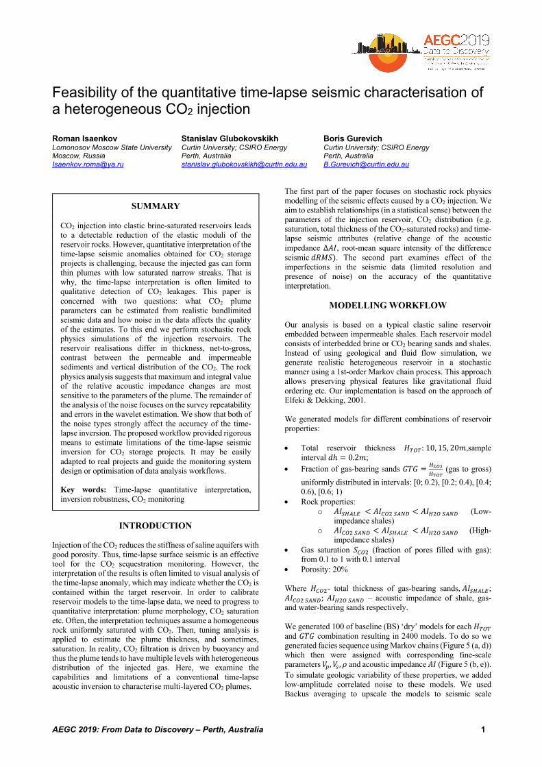
• Main time-lapse seismic attributes (Figure 1):

o 𝑑𝑅𝑀𝑆 = 𝑅𝑀𝑆P+ − 𝑅𝑀𝑆N> o Δ𝐴𝐼P?R – maximum of time-lapse impedance

anomaly Δ𝐴𝐼 o Δ𝐴𝐼SE+ = ∑ Δ𝐴𝐼 ⋅ 𝑑ℎV∈[Y;9=;=] - the area under Δ𝐴𝐼

curve o 𝐻A[ =

\?]^=\?S_`a

- equivalent thickness

Figure 1. Illustration of time-lapse seismic attributes

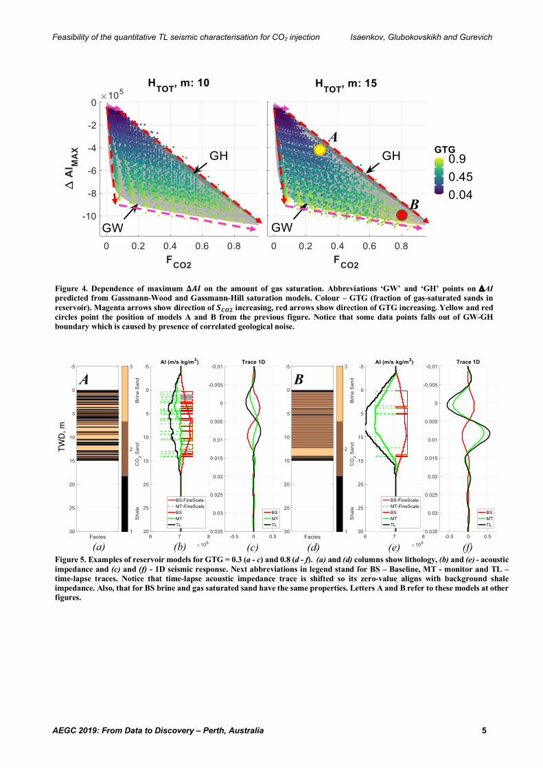
We found a strong linear relationship between Δ𝐴𝐼SE+ and 𝐻C,D. However, Δ𝐴𝐼SE+ is much less sensitive to saturation. As demonstrated by Figure 4, Δ𝐴𝐼P?R − 𝐹C,D relationship cannot be described by uniform Gassmann-Wood or patchy Gassmann-Hill equations – values fall somewhere in between depending on 𝑆C,D. The less gas saturation of sands – the closer

Δ𝐴𝐼P?R to Gassmann-Wood boundary and wise versa. For a vertically ‘smeared’ plume, the results plot closer to the Gassmann-Hill limit. In this study we show only attributes listed above as they are most important; however many other useful attributes may exist.

INFLUENCE OF THE SEISMIC NOISE In the first section, we focused on the sensitivity of seismic data to reservoir parameters . In this section, our goal is to estimate how robust seismic inversion at reconstruction ‘true’ Δ𝐴𝐼 is in the presence of additive noise and wavelet estimation errors. By ‘true’ Δ𝐴𝐼, we mean Backus averaged acoustic impedance as ‘ideal’ result of inversion analysed in the perevious section. Inversion of noisy traces was divided into two steps: first, noise-contaminated traces were generated for BS and MT traces with the same noise level but different realisations; secondly, these traces were deconvolved with the original wavelet 𝑆(𝑡) and integrated to 𝐴𝐼P+d and 𝐴𝐼N>d . Their difference is Δ𝐴𝐼d. To simulate inversion errors, we introduce two types of noise into inverted traces: band-limited additive aquisition noise 𝑊?FFand wavelet estimation errors 𝑊f?gA. To determine noise-free seismic trace 𝐺(𝜔) for reflection coeffitients 𝑅ii(𝜔) and wavelet 𝑆(𝜔) we use matrix propagator operator. Then, with some simplification, the resulting trace is:

𝐺(𝜔) = 𝑅ii(𝜔) ⋅ 𝑆(𝜔) Application of the Tikhonov regularised deconvolution then converts the seismic trace into reflection coefficients. Even this relatively simple inversion process highly depends on the regularisation parameter. For each model in Figure 5, we have chosen those parameters which produce the least error (~ 5%) in comparison with the ‘true’ AI model.

𝑅II(𝜔) = 𝐺(𝜔) ⋅ 𝑆jk(𝜔) Acquisition noise is Gaussian noise Vmnn(𝜔) with RMS level equal to one whose frequency band is limited to that of the wavelet spectrum Vmnn(𝜔). This noise is scaled by 𝑅𝑀𝑆oAp to have the same level amplitudes as background reflections form similar rock types and multiplied by 𝑁?FF to produce the required noise level. With this notation, SNR might be calculated as 𝑆𝑁𝑅?FF = 1/𝑁?FF 𝑅𝑀𝑆oAp is RMS amplitude level of traces modelled for background CO2-free rocks consisting of brine-sand and shale sequence. This parameter is different for models with high-impedance shales (𝑅𝑀𝑆oAp = 0.07) and low-impedance shales (𝑅𝑀𝑆oAp = 0.18) which reflects different contrast at the sand-shale boundary,

𝑊?FF(𝜔) =𝑁?FF ⋅ 𝑅𝑀𝑆oAp ⋅ Vmnn(𝜔) where 𝑊f?gA(𝜔) is scaled Gaussian band-limited noise with

unit RMS level, 𝑉f?gA(𝜔). 𝑁f?gA = uv AwAxy`xz

{ is the square

root of spectral energy of signal 𝐸> and noise 𝐸gy`xz.

Feasibility of the quantitative TL seismic characterisation for CO2 injection Isaenkov, Glubokovskikh and Gurevich

AEGC 2019: From Data to Discovery – Perth, Australia 3

𝑊f?gA(𝜔) = 𝑁f?gA ⋅ 𝑉f?gA(𝜔) Then we used corrupted wavelet 𝑆d and additive noise 𝑊?FF to produce corrupted trace 𝐺d which is inverted to get erroneous reflection coefficients 𝑅IId (𝜔). Notice that for inversion we used operator 𝑆jk based on noise-free wavelet for both BS and MT.

𝑆d(𝜔) = 𝑆(𝜔) +𝑊f?gA(𝜔) 𝐺d(𝜔) = 𝑅II(𝜔) ⋅ 𝑆d(𝜔) +𝑊?FF(𝜔)

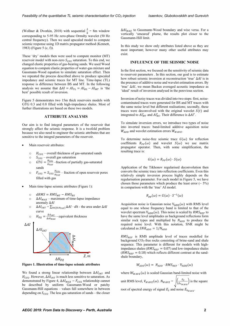
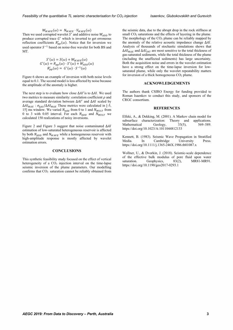
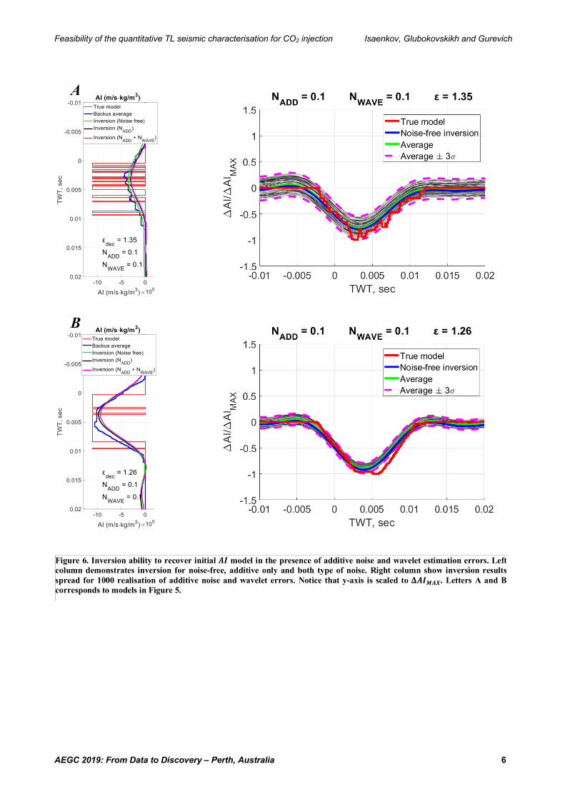
𝑅IId (𝜔) = 𝐺d(𝜔) ⋅ 𝑆jk(𝜔) Figure 6 shows an example of inversion with both noise levels equal to 0.1. The second model is less affected by noise because the amplitude of the anomaly is higher. The next step is to evaluate how close Δ𝐴𝐼dis to Δ𝐴𝐼. We used two metrics to measure similarity: correlation coefficient 𝜌 and average standard deviation between Δ𝐴𝐼d and Δ𝐴𝐼 scaled by Δ𝐴𝐼P?R : 𝜎\?S/Δ𝐴𝐼P?R These metrics were calculated in [-5, 15] ms window. We varied 𝑁��� from 0 to 1 and 𝑁P�@+ from 0 to 3 with 0.05 interval. For each 𝑁?FF and 𝑁P�@+ we calculated 150 realizations of noisy inversions. Figure 2 and Figure 3 suggest that noise contaminated Δ𝐴𝐼 estimation of low-saturated heterogeneous reservoir is affected by both 𝑁?FF and 𝑁f?gA while a homogeneous reservoir with high-amplitude response is mostly affected by wavelet estimation errors.

CONCLUSIONS This synthetic feasibility study focused on the effect of vertical heterogeneity of a CO2 injection interval on the time-lapse seismic inversion of the plume parameters. Our modelling confirms that CO2 saturation cannot be reliably obtained from

the seismic data, due to the abrupt drop in the rock stiffness at small CO2 saturations and the effects of layering in the plume. The morphology of the CO2 plume can be reliably mapped by the anomaly of the relative acoustic impedance change Δ𝐴𝐼. Analysis of thousands of stochastic simulations shows that Δ𝐴𝐼P?R and Δ𝐴𝐼SE+are most sensitive to the total thickness of gas-saturated sediments, while the total thickness of the plume (including the unaffected sediments) has large uncertainty. Both the acquisition noise and errors in the wavelet estimation have a strong effect on the time-lapse inversion for low-saturated plume, while only the wavelet repeatability matters for inversion of a thick homogeneous CO2 plume.

ACKNOWLEDGEMENTS The authors thank CSIRO Energy for funding provided to Roman Isaenkov to conduct this study, and sponsors of the CRGC consortium.

REFERENCES Elfeki, A., & Dekking, M. (2001). A Markov chain model for subsurface characterization: Theory and applications. Mathematical Geology, 33(5), 569–589. https://doi.org/10.1023/A:1011044812133 Kennett, B. (1983). Seismic Wave Propagation in Stratified Media. In Cambridge University Press. https://doi.org/10.1111/j.1365-246X.1986.tb01087.x Wollner, U., & Dvorkin, J. (2018). Seismic-scale dependence of the effective bulk modulus of pore fluid upon water saturation. Geophysics, 83(2), MR81-MR91. https://doi.org/10.1190/geo2017-0293.1

Feasibility of the quantitative TL seismic characterisation for CO2 injection Isaenkov, Glubokovskikh and Gurevich

AEGC 2019: From Data to Discovery – Perth, Australia 4

Figure 2. Correlation coefficient between inverted and initial AI model in the presence of additive noise 𝑵𝑨𝑫𝑫 and wavelet estimation errors. 𝑵𝑴𝑼𝑳𝑻. Letters A and B corresponds to models in Figure 5. Purple line is intersection of surface with correlation coefficient = 0.85. Gaussian averaging was applied to image.

Cor

rela

tion

coef

ficie

nt

A B

Figure 3. Scaled average deviation of inverted AI in presence of additive noise 𝑵𝑨𝑫𝑫 and wavelet estimation errors𝑵𝑴𝑼𝑳𝑻. Letters A and B corresponds to models in Figure 5. Purple line is intersection of surface with correlation coefficient = 0.85. Gaussian averaging was applied to image.

𝜎 \?S

Δ𝐴𝐼 P

?R

𝜎\?SΔ𝐴𝐼P?R

A B

Feasibility of the quantitative TL seismic characterisation for CO2 injection Isaenkov, Glubokovskikh and Gurevich

AEGC 2019: From Data to Discovery – Perth, Australia 5

Figure 4. Dependence of maximum 𝚫𝑨𝑰 on the amount of gas saturation. Abbreviations ‘GW’ and ‘GH’ points on DAI predicted from Gassmann-Wood and Gassmann-Hill saturation models. Colour – GTG (fraction of gas-saturated sands in reservoir). Magenta arrows show direction of 𝑺𝑪𝑶𝟐 increasing, red arrows show direction of GTG increasing. Yellow and red circles point the position of models A and B from the previous figure. Notice that some data points falls out of GW-GH boundary which is caused by presence of correlated geological noise.

A

B

TWD,

m

Figure 5. Examples of reservoir models for GTG = 0.3 (a - c) and 0.8 (d - f). (a) and (d) columns show lithology, (b) and (e) - acoustic impedance and (c) and (f) - 1D seismic response. Next abbreviations in legend stand for BS – Baseline, MT - monitor and TL – time-lapse traces. Notice that time-lapse acoustic impedance trace is shifted so its zero-value aligns with background shale impedance. Also, that for BS brine and gas saturated sand have the same properties. Letters A and B refer to these models at other figures.

A B

(a) (b) (c) (d) (e) (f)

Feasibility of the quantitative TL seismic characterisation for CO2 injection Isaenkov, Glubokovskikh and Gurevich

AEGC 2019: From Data to Discovery – Perth, Australia 6

B

A

Figure 6. Inversion ability to recover initial 𝑨𝑰 model in the presence of additive noise and wavelet estimation errors. Left column demonstrates inversion for noise-free, additive only and both type of noise. Right column show inversion results spread for 1000 realisation of additive noise and wavelet errors. Notice that y-axis is scaled to 𝚫𝑨𝑰𝑴𝑨𝑿. Letters A and B corresponds to models in Figure 5.