1

3D Time-lapse Seismic Modeling for CO2 Sequestration

Jintan Li Advisor: Dr. Christopher Liner

April 29th, 2011

2

Outline

• Background/Introduction

• Methods

• Preliminary Results

• Future Work

3

Goal

Flow simulation for time-lapse seismic modeling

To monitor:

– CO2 movement and containment

– Long term CO2 stability

To evaluate:

– Effectiveness of 4D seismic (CO2 injection causes change of seismic response)

4

Flow Simulation

- Simulate liquid and gas flow in real world conditions

- Generalized equation of state compositional simulator (GEM)- by CMG (computation modeling group). Used for:

- CO2 capture and storage (CCS)

- CO2 enhanced oil recovery

Geology (reservoir)

Flow simulation Seismic modeling

5

Vp,Vs, density calculation via Gassmann’s Equation

Reservoir flow simulation cell

Geological grid Seismic grid

1D forward modeling : convolutional model

Petrel modeling : porosity,

permeability

In each grid cell: fluid properties

Input top maps and thickness isopachs,

porosity and permeability from the petrel model

Depth-time conversion: Time-Depth table from well log

Upscale to seismic bin size (x and y direction)

Calculate reflectivity at zero offset

seismic scale

reservoir scale

Log scale

Calibration

6

Background

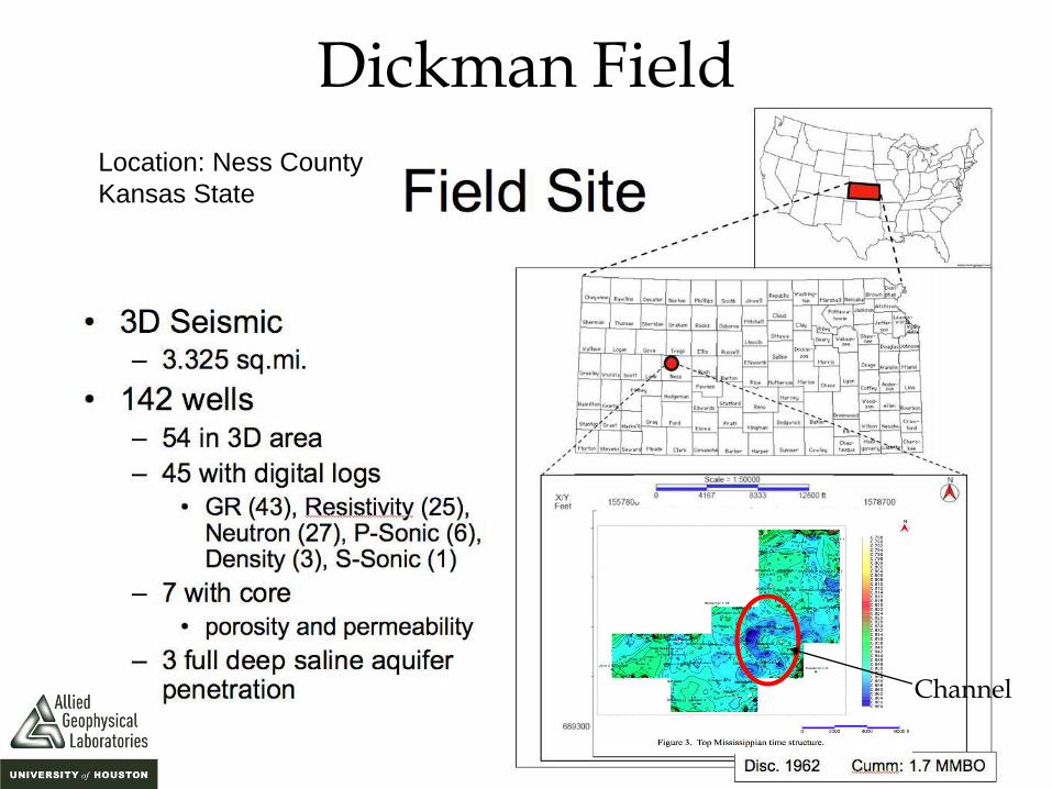
• Study area: Dickman Field, Kansas

• Geology: carbonate build-ups, karst feature

• Two CO2 capture and storage targets • Deep Saline Aquifer - primary

• Shallower depleted oil reservoir - secondary

7

Dickman Field

Location: Ness County

Kansas State

Channel

8

CO2 Properties

• Reservoir conditions at Dickman Field: Temperature: 31.7-48.8339°C

Pressure: 8.53~16.25mpa

• CO2: Supercritical fluid beyond dynamic critical point : (T>31.1°C & P >7.38 MP, Density: >0.469 g/cm3) Gas phase Liquid phase

(Han et al., 2010)

Dickman field CO2

9

PermK (md)

Sim Layer No. VerticalPerm Porosity(%) Formation Name

1-6 10 md 18.2 Shallow Reservoir layers

7-8 0.01 md 20.0 Two Seal Layers

9-10 0.7 Horizontal Perm 10.3 Ford Scott Limestone

11-13 0.5 Horizontal Perm 19.1 Cherokee

14-15 0.5 Horizontal Perm 16.5 Lower Cherokee

16 0.7 Horizontal Perm 14.8 Mississippian Unconformity

17-20 0.7 Horizontal Perm 20.0 Mississippian Porous Carbonate

25-32 0.7 Horizontal Perm 22.45 Mississippian Osage and Gillmor City

32 simulation layers

Flow simulation grid

NX=33 dx=500ft; NY=31 dy=500ft; NZ=32, dz: variable

Flow Simulation Model (vertical)

x

z

Perm K (md)

10

CO2 monitoring Scenario: CO2 is injected for 50 yrs, then the injection well is

shut in and flow modeling continues for 150 yrs Input: • Fluid simulation results for 150 yrs: (2002’-2155’) grid cells: 33(x)*31(y)*32(z) dx=500ft, dy=500ft, dz: variable fluid properties data (porosity, CO2 saturation, etc.)

Output: • Seismic simulation for 150yrs - implemented by MATLAB: binary file - Seismic Unix: headers correctly added and sorted and interpolated

into the field seismic data bin size(82.5ft x 82.5ft) • Comparison of seismic response due to CO2 injection (between year

2002’ and 2155’)

inline 86 and

xline 98

Figure 1. CO2 saturation for simulation layers from 1 through 16 for years 2002 (L) and 2155 (R). Two seismic lines (inline 86 and crossline 98) in sim layer 9 have been pulled out for comparison.

CO2 Saturation for Sim Layers 1-16 (Yr 2002’ and 2155’)

Figure 3a. Seismic data (inline86) at the different simulation time (2002’ and 2150’) and the difference. Displayed from 500ms to 800ms. It caused 4% impedance change.

Seismic Data Inline 86 (Yr 2002’ and 2155’) and Difference

Figure 3b. Seismic data (crossline 98) at the different simulation time (2002’ and 2155’) and the difference. Displayed from 500ms to 800ms.

Seismic Data Xline 98 (Yr 2002’ and 2155’) and Difference

14

Future Work

• To perform a full wave forward modeling to obtain more realistic result

• A smoother and better-defined porosity distribution may help improve the seismic data quality

15

Acknowledgement

• Dr. Christopher Liner (Principle Investigator)

• Po Geng (Flow simulation)

• June Zeng (Geologist)

• CO2 Team • Qiong Wu

• Shannon Leblanc

• Johnny Seals

• Tim Brown

• Eric Swanson

16

END

Extra slides

18

Geology Model Petrel modeling:

- faults interpretation constrained by seismic volume attributes

- up-scaled log porosity based on lithozones

- relationship between:

1) core porosity and log porosity

2) core porosity and permeability

3) seismic impedance and neutron porosity

permeability

Guiding propagation of permeability in property modeling

(Zeng,2009)

CO2 Storage

• T=121F & P=2200 psi :

Density=0.7 ton/m^3

Brine solubility= 64 ton per acre-ft

• Porosity=0.2, Sw=20%, CO2 trapped in 1 acre-ft :

1233(m^3 per acre-ft)*0.2*(1-0.2)*0.7 ton/m^3=140 tons

20

Dickman Field

Acreage = 240 acres Net Pay Zone Thickness = 7 feet Average depth = 4424 feet in MD Oil API gravity = 37 API (0.84 g/cm3) The reservoir average temperature = 113 ° F The reservoir average pressure = 2066 psi TDS (Total Dissolved Solid) salinity = 45,000 ppm

21

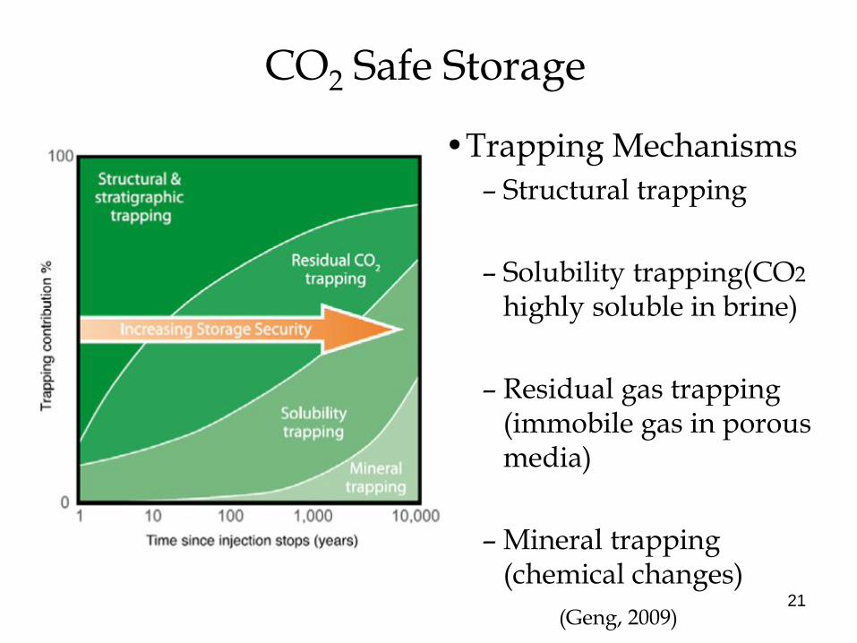
CO2 Safe Storage

•Trapping Mechanisms

– Structural trapping

– Solubility trapping(CO2 highly soluble in brine)

– Residual gas trapping (immobile gas in porous media)

– Mineral trapping (chemical changes)

(Geng, 2009)

22

Flow Simulation Model

Acquifer model (from top to base)

1. Fort Scott Limestone

2. Cherokee Group

3. Lower Cherokee Sandstone

4. Mississippian Carbonate

5. Lower Mississippian Carbonate

CO2 storage target

CO2 storage target

b) a) CO2 saturation, inline86 Porosity distribution, inline86

Figure 2. Vertical sections related to inline 86 for year 2155.

(a) Porosity distribution. (b) CO2 saturation

24

Discussion

After CO2 being injected for 150yrs,

at the location where has the highest change for CO2 saturation:

Sco2 change: 0%~42%

Impedance change: 4%

Reflection coefficient change: 41% (non-linear)