HAL Id: hal-01372057https://hal.archives-ouvertes.fr/hal-01372057

Submitted on 26 Sep 2016

HAL is a multi-disciplinary open accessarchive for the deposit and dissemination of sci-entific research documents, whether they are pub-lished or not. The documents may come fromteaching and research institutions in France orabroad, or from public or private research centers.

L’archive ouverte pluridisciplinaire HAL, estdestinée au dépôt et à la diffusion de documentsscientifiques de niveau recherche, publiés ou non,émanant des établissements d’enseignement et derecherche français ou étrangers, des laboratoirespublics ou privés.

Fatigue life under non-Gaussian random loading fromvarious models

Alexis Banvillet, T. Lagoda, E. Macha, A. Nieslony, Thierry Palin-Luc, J-F.Vittori

To cite this version:Alexis Banvillet, T. Lagoda, E. Macha, A. Nieslony, Thierry Palin-Luc, et al.. Fatigue life undernon-Gaussian random loading from various models. International Journal of Fatigue, Elsevier, 2004,26, pp.349-363. �10.1016/j.ijfatigue.2003.08.017�. �hal-01372057�

Fatigue life under non-Gaussian random loading from variousmodels

A. Banvillet a, T. Łagoda b,∗, E. Macha b, A. Niesłony b, T. Palin-Luc a, J.-F. Vittori ca E.N.S.A.M. CER de Bordeaux, Laboratoire Materiaux Endommagement Fiabilite et Ingenierie des Procedes (EA 2727),

Esplanade des Arts et Metiers, F-33405 Talence Cedex, Franceb Technical University of Opole, Dept. Mechanics and Machine Design, ul. Mikołajczyka 5, 45-271 Opole, Poland

c Renault, Technocentre, Dir. Ingenierie des Materiaux, Sce 64130, API : TCR LAB 035, 1 Av. Golf, F-78288 Guyancourt Cedex, France

Abstract

Fatigue test results on the 10HNAP steel under constant amplitude and random loading with non-Gaussian probability distribution function, zero mean value and wide-band frequency spectrum have been used to compare the life time estimation of the models proposed by Bannantine, Fatemi–Socie, Socie, Wang–Brown, Morel and Łagoda–Macha. Except the Morel proposal which accumu-lates damage step by step with a proper methodology, all the other models use a cycle counting method. The rainflow algorithm is used to extract cycles from random histories of damage parameters in time domain. In the last model, where a strain energy density parameter is employed, additionally spectral method is evaluated for fatigue life calculation in the frequency domain. The best and very similar results of fatigue life assessment have been obtained using the models proposed by Socie and by Łagoda–Macha, both in time and frequency domains for the last one.

Keywords: Fatigue life calculation; Strain energy; Spectral method; Rainflo algorithm; Random loading

1. Introduction

The known algorithms for assessment of fatigue lifeof machine components and structures under randomloading can be divided into two groups. Some of themuse numerical methods for cycle counting and damageaccumulation step by step. On the other group, there arethe so called ‘spectral methods’ based on the spectralanalysis of stochastic processes. In the firs group, theloading of the material is usually represented by timecourses of stresses and/or strains, and in the other groupby their frequency characteristics, i.e. by the power spec-tral density function or its parameters. Lately [1–4], thestrain energy density parameter has been proposed forfatigue life evaluation. This parameter seemed to beefficien in the case of fatigue life determination basedon a cycle counting method [1,2,4]. The energy para-

∗ Corresponding author. Tel.: +48-77-4006-198; fax: +48-77-4006-343.

E-mail address: tlag@po.opole.pl (T. Łagoda).

0142-1123/$ - see front matter 2003 Elsevier Ltd. All rights reserved.doi:10.1016/j.ijfatigue.2003.08.017

meter includes the strain and stress histories and keepsthe frequency character of the loading. Thus, we mayask if the strain energy density parameter can be appliedin spectral methods where the power spectral densityfunction plays the most important role.The algorithms of fatigue life determination under

multiaxial random loading must be also valid for the uni-axial random stress state. In a particular case, elementsof machines and structures can remain in such a stressstate for a certain life time. Verificatio of the model ofmultiaxial fatigue only for the uniaxial stress stateincludes one of the important stages of correctness thesealgorithms. This paper deals with the comparison ofsome selected models of fatigue life estimation understationary non-Gaussian random axial loading on thebasis of experimental data obtained for the 10HNAPsteel in high cycle fatigue (HCF). In this paper the fol-lowing models for multiaxial loading are analyzed andtheir predictions compared with experiments: Smith–Watson–Topper damage parameter used by Bannantine–Socie [5], Fatemi–Socie [5,6], Socie for HCF [7], Wang–Brown [8,9], Morel [10,11] and Łagoda–Macha [1–4].

Nomenclature

AW = Wm’a N fatigue curve in an energy approach

a’ for the energy approach, coeff cient allowing to include cycles with amplitudes below the fatiguelimit from an arbitrary stress level

A = smaN fatigue curvea coeff cient allowing to include stress amplitudes below the fatigue limitb tensile fatigue strength exponentb0 shear fatigue strength exponentc tensile ductility exponentc0 shear fatigue ductility exponentE Young modulus of the material

M + = �l4l2 expected number of peaks in a time unit

G shear modulus of the materialG(f) power spectral density functionm slope of the Wohler curve,m’ = m /2 slope of the energy fatigue curveNo number of cycles corresponding to the fatigue limitNf number of cycles to failureni number of cycles with a stress amplitude sai>n(q,f) unit normal vector to a material plane orientated by the angles q, j (spherical coordinates)p, q, r material parameters of the Morel approachPn→ material plane orientated by >n(q,f)q1 asymmetry or skewnessq2 excessTBa life calculated according to the Bannantine–Socie modelTCh-D,W life (in s) calculated according to the Chaudhury–Dover model with strain energy density parameterTexp experimental fatigue lifeTFS life calculated according to the Fatami–Socie modelTMo life calculated according to the Morel modelTRF,W life calculated according to cycle counting algorithm from strain energy density parameter historyTRMS root mean square value of the macroscopic resolved shear stressTSo life calculated according to the Socie modelTWB life calculated according to the Wang–Brown modelTo observation timex, y, z axis linked with the specimenx�, y�, n arbitrary axis linked with the critical plane orientated by

>n(q,f)

W strain energy density parameter, distinguishing tension and compression,Waf fatigue limit according to the energy parameter

a =l2

√l0l4coeff cient of irregularity

��f tensile fatigue ductility coeff cientg = √1�a2 coeff cient of the spectrum widthg �f shear fatigue ductility coeff cient�(x) gamma functionn Poisson’s ratiot�f shear fatigue strength coeff cients�f axial fatigue strength coeff cientq,f angles orientating

>n in spherical coordinates system

ms = l0 variance of a stress history s(t)sa max maximum amplitude in the history of stress after cycle counting by means of the rainf ow algorithm

saf fatigue limit in fully reversed tension–compressiony angle, from f xed axis in the plane Pn→, to def ne the direction where the resolved shear stress is

computed

lk = ��

0fkG(f)df kth moment of one-sided power spectral density function of the stress history s(t)

In the last model the strain energy density parameter isused both in time and frequency domain. In the f rst fourmodels the damage parameter used has been originallyproposed for cyclic loading, then used by some authorsfor variable amplitude multiaxial loading [5]. One aimof this paper is also to investigate if such models shouldbe valid also for uniaxial random loading.

2. Comments about the methods using a cyclecounting algorithm and based on the critical planeapproach

With a general point of view, all the fatigue life calcu-lation methods using a cycle counting algorithm can besummarized with the same methodology. First a cyclecounting variable is chosen in order to extract the cycles(with their amplitude and mean value) from the variableamplitude or random multiaxial loading signal (stressesand/or strains). For the simulations presented hereafterthe ASTM rainf ow algorithm was used [13] (with 64classes). All the random loadings are considered asstationary for life calculation. Secondly, a damage para-meter Dp is chosen; it depends on stress-strain quantities.This damage parameter is computed on each materialplane Pn→, orientated by the unit normal vector

>n(q,f)

(Fig. 1), in order to look for the critical plane Pn→c. Notethat since the fatigue critical point is at the specimensurface the stress state is plane at this location, thus the

Fig. 1. Coordinates system used to def ne the unit normal vector >norientating each material plane Pn→ at the point M on the surface ofthe specimen.

number of planes to examine to look for the critical onecan be reduced. All the computations were done by con-sidering that q = 45° and 90°, for f varying between 0°and 180° as proposed in ref. [9,14]. Thirdly, to quantifythe damage generated by each cycle identif ed with thecounting algorithm it is necessary to use an equationrelating the damage parameter and the number of cyclesto failure Nf under constant amplitude loading. It is thenpossible to compute the elementary damage caused byeach extracted cycle and to accumulate step by step thisdamage by using, for instance, the linear Palmgren–Miner rule. Small cycles with a stress amplitude generat-ing an elementary damage smaller than 10�12 were neg-lected in our computations. According to the S–N curveof the tested material, it corresponds to a stress ampli-tude smaller to 0.25 saf in fully reversed tension. Finally,the fatigue life is calculated by assuming a thresholdvalue of the total damage sum. One is usually used forthis threshold value as it was done in this paper, butsome authors have shown that this limit can vary in alarge interval [15,16].

3. Fatemi and Socie’s model

According to Fatemi and Socie (FS) [5–7], for eachmaterial plane Pn→, the cycle counting method has to beapplied on two variables: the shear strains gnx’(t) andgny’(t). The critical plane is, for each of these two coun-ting variables, the plane experiencing the highest shearstrain range. For the materials where the fatigue crackinitiation is dominated by plastic shear strains FS rec-ommend to use the following damage parameter: DpFS= ga(1 + k1sn,max /sy) related to the Manson–Coff n curvein torsion by equation:

ga(1 � k1sn,max /sy) �t�fG (2Nf)

b0 � g�f(2Nf) c0. (1)

The term on the left-hand side represents the damageparameter on the critical plane. For each loading cycleextracted by the rainf ow method, ga is the shear strainamplitude (�gnx� /2 or �gny� /2). sn,max is the maximumof the normal stress on the critical plane, during the cur-rent cycle of the counting variable gnx�(t) or gny�(t) (Fig.2). sy is the yield stress of the material in tension. Inthis damage parameter, k1 is a material constant ident-if ed by f tting uniaxial against pure torsion fatigue data.

Fig. 2. Def nition of the mean and maximum normal stress during anextracted cycle (from t1 to t2) with the rainf ow algorithm.

The right-hand side of Eq. (1) is the description of thestrain-life Manson–Coff n curve in torsion. When thestrain-life Manson–Coff n torsion curve is not known,FS propose to approximate this curve from the tensilestrain-life curve [6]. The algorithm used to apply thisfatigue life calculation method is detailed in a f ow chartin Appendix 1.

4. Smith–Watson–Topper parameter used byBannantine and Socie

For the materials where short fatigue cracks grow onthe plane perpendicular to the maximum principal stressand strain (mode I), Bannantine and Socie [5] rec-ommend using the Smith–Watson–Topper (SWT) dam-age parameter: DpSWT = en,asn,max. For each materialplane Pn→, the cycle counting method is applied on thenormal strain en(t). The relation between the damageparameter and the number of cycles to failure Nf for aconstant amplitude loading in tension is:

en,asn,max �s�2fE (2Nf) 2b � s�fe�f(2Nf) b+c (2)

In this equation and for each load cycles extracted bythe rainf ow method, en,a is the amplitude of the normalstrain and sn,max is the maximum normal stress duringthe current cycle of the counting variable en(t) (Fig. 2).The algorithm used to compute life according to thismodel is shown in Appendix 2.

5. Socie’s proposal for HCF regime

According to Fatemi and Socie for HCF and ductilematerials most of the fatigue life is consummed by cracknucleation on the planes where the shear stress is

maximum. In this case Socie [7] proposes the followingstress based approach by using as damage parameter:DpSo = ta + k2sn,max. This is the linear combination ofthe shear stress amplitude ta and the maximum normalstress sn,max, acting on the critical plane, both during theload cycle (Fig. 2). For each material plane Pn→, the cyclecounting algorithm has to be applied on two countingvariables: the shear stresses tnx�(t) and tny�(t). The criticalplane is, the plane experiencing the highest shear stressrange (�tnx�(t) or �tny�(t)). The relation linking the dam-age parameter and the number of cycles to failure underconstant amplitude loading is given by the followingequation:

ta � k2sn,max � t�f(2Nf)b0. (3)

The right-hand side of this equation is the elastic part ofthe strain-life curve. k2 is a material parameter identif edby f tting tension and torsion fatigue data. The algorithmused to apply this method is illustrated in Appendix 3.

6. Wang and Brown’s model

Wang and Brown [8,9] developed a model f rst restric-ted to low cycle fatigue (LCF) and medium cycle fatigue(MCF) according to the assumption that fatigue crackgrowth is controlled by the maximum shear strain. Foreach material plane Pn→, the rainf ow cycle countingmethod has to be applied on two counting variables: theshear strains gnx�(t) and gny�(t). The critical plane is theplane experiencing the highest shear strain range.Assuming that, during one cycle the normal strain excur-sion �en plays an important additional role, Wang andBrown propose the following expression as damageparameter: DpWB = ga + S �en, where ga is the shearstrain amplitude and S is a material parameter identif edby f tting tension against torsion fatigue data. Therelation between the damage parameter and the life timeis expressed as

ga � S �en � (1 � ne � S(1�ne))s�f�2sn,mean

E (2Nf) b

� (1 � np � S(1�np)) e�f(2Nf) c (4)

where ne and np are respectively the elastic and plasticPoisson’s ratio of the material. sn,mean is the mean nor-mal stress on the critical plane during each extractedcycle (Fig. 2) of counting variable gnx�(t) or gny�(t).The algorithm used to compute the fatigue life accord-

ing to the Wang–Brown model is shown in Appendix 4.

7. Morel’s approach

Morel developed a model for polycrystalline metalsin HCF based on the mesoscopic plastic strain accumu-

lation [10,11,12]. This author assumes that the mechan-ical behaviour of each grain of the material follows athree phase law: hardening, saturation and softening. Themesoscopic plastic strain � is chosen as a damage para-meter. By assuming that each crystal of the materialobeys to a combined isotropic and kinematic hardeningrule when f owing plastically, the initiation of slip ineach grain is described by the Schmid criterion. Accord-ing to Morel a fatigue crack initiates if the cumulatedmesoscopic plastic strain reaches a critical value �fdepending on the material. For multiaxial constantamplitude loading Morel uses the high cycle multiaxialfatigue criterion proposed by Papadopoulos, who dem-onstrated that the limit value of the Ts parameter (whichis an upper bound value of the plastic mesostrainaccumulated in some crystals of an elementary volumeV) is depending on the maximum value of the hydrostaticstress H,max during a loading cycle

maxq,jTs(q,j) � aH,maxb (5)

In this approach the critical plane, orientated by theunit normal vector def ned by the angles (q,j), is theplane experiencing the maximum value, noted T, ofTs(q,j). From this criterion, Morel def nes a limit multi-axial loading (so that Tlim + aH,max,lim = b) dependingon both the amplitude H,a and the mean value H,m ofthe hydrostatic stress

Tlim ��aH,m � bT

a �T

H,a

·T

H,a(6)

Then from the macroscopic shear stress amplitude CAacting on the critical plane, the limit value tlim of themesoscopic shear stress during the saturation phase isequal to the ratio Tlim /H where H is a ‘phase-differenceparameter’: H = T /CA. Finally, from the hypothesis thata fatigue crack initiates on the critical plane in the moststressed grains, Morel proposed the following S–N curveequation, for constant amplitude loadings

Nf � p ln� CACA�tlim� � q � tlim

CA�tlim� �rCA

(7)

where p, q and r are three material parameters (functionof the hardening, saturation and softening phases of thecrystal) which can be identif ed from only one experi-mental S–N curve.Under variable amplitude loading, the amplitude,

mean value and phase difference of each stress ij(t) cannot be def ned. In this case, to simplify the fatigue lifeprediction problem Morel proposed to consider as criti-cal plane, the most damaging one. One way to localizethis plane is to look for the maximum value ofTs,RMS(q,f) (noted T,RMS), which is the root meansquare of the macroscopic resolved shear stress actingon a line orientated by the unit vector

>m(y). This unit

vector is determined by the angle y from f xed axis inthe plane def ned by its angles θ and φ (sphericalcoordinates) [10,11].

T,RMS � maxq,fTs,RMS(q,f) with Ts,RMS(q,f)

� ��2py � 0

T2RMS(q,f,y)dy (8)

Once the critical plane located, the ‘phase parameter’H is computed with equation

H �TRMS

CRMSwhere CRMS � max

yTRMS(y) (9)

on this plane (Appendix 5).After this step, the time history of the hydrostatic

stress H(t) and of the resolved shear stress t(y,t)on thecritical plane is computed. The amplitude of the hydro-static stress and its mean value between two extreme atti and ti+1 of the macroscopic resolved shear are respect-ively: H,a = |H(ti + 1)�H(ti)| /2 and H,m = (H(ti) +H(ti + 1)) /2. The amplitude of the resolved shear stressis ta(y) = |ta(y,ti + 1)�ta(y,ti)| /2. By assuming that T

/ta(y) (for each transition ti to ti+1) and H = TRMS /CRMS (for all the load sequence) are the same; T is com-puted for the current transition by: T = H ta(y). Thus,for each transition, the application of Eq. (6) allows usto estimate the limit value of the mesoscopic shear stress

with tlim =Tlim

TRMS /CRMSfor the direction >m(y). Finally,

the saturation yield limit of the crystal, in this directionof the critical plane, can be estimated from the meanvalue (tlim)mean (calculated over the whole sequence) ofthe saturation shear stress at each loading transition. Thiscalculation is done over each direction of the criticalplane; the number of sequences to fatigue crack initiationis deduced from the direction leading to the highestaccumulated damage. Note that for the Morel methodthe damage accumulation is done step by step withoutany cycle counting method (rainf ow for instance)according to the rules described in the following para-graph. Thus, the calculated life is sensitive to the orderof the stress levels.To apply this calculation method the parameters p =

c + m4 (1/g + 1/h), q, r= q

t(0)yg of the S–N curve (7) are

necessary but the initial yield stress of the crystal t(0)y isalso needed to be able to cumulate damage. The identi-f cation of these four parameters requires a specif c dam-age cumulative fatigue test (detailed in [11]) to identifyseparately the hardening parameter g. Damage is cumu-lated according to the following rules. During the hard-

ening phase ty =1

c + mg + 1

√t·t, and during the softening

phase ty =1

1 �c + mh

√t·t. If the yield stress of the crys-

tal ty is equal to tlim the saturation phase is reached.Then, the softening phase begins as soon as � =4qtlim where � = √t·t. Fatigue crack initiates in the grainwhen the crystal yield stress reaches zero.

8. The strain energy density parameter

A change of strain energy density, applied in theory ofplasticity, has been proposed as a parameter to describemultiaxial fatigue [1–4]. In order to distinguish the workunder tension and compression during a uniaxial fatiguecycle, Łagoda and Macha introduce the functionssgn[s(t)] and sgn[e(t)] as follows,

W(t) �12s(t)e(t)

sgn[s(t)] � sgn[e(t)]2 (10)

where

sgn[x] � � � 1 for x � 00 for x � 0�1 for x 0

,

s(t), e(t) are stress and strain time history in the criticalplane. For uniaxial loading it means s(t) = sx(t) ande(t) = ex(t).Eq. (10) expresses positive and negative values of the

strain energy density parameter in a fatigue cycle and itallows to distinguish energies under tension and com-pression. If this parameter is positive, the material is sub-jected to tension. When it is negative, the material issubjected to compression. Eq. (10) has another advan-tage: energy course in time has the zero mean valuewhen cyclic stresses and strains change symmetricallyin relation to the zero levels.If the cyclic stresses and strains reach their maximum

values sa and �a, the maximum value of the energy para-meter (10) and its amplitude are the same: Wa = Wmax.

Wa �12saea (11)

Assuming W(t) according to Eq. (10) as a fatigue failureparameter, the standard characteristic curves of cyclicfatigue (sa�Nf) and(ea�Nf) can be rescaled to obtain anew curve, (Wa�Nf). In the case of high-cycle fatigue,when the characteristic (sa�Nf) is used, the sa axisshould be replaced by Wa, where

Wa �s2a2E. (12)

So we obtain,

Wa �(s’f)2

2E (2Nf)2b �(s’f)2

2E (2Nf)b’ (13)

From among the cyclic counting methods, the rainf owalgorithm and the Palmgren–Miner hypothesis of dam-age accumulation have been chosen [1,2,4]. The lifetime, TRF is calculated from cycles and half-cycles in thetime observation To of stress history s(t),

TRF �To

�ki � 1

[ni /(No(saf /sai)m)]for sai� a saf,a � 0.5 (14)

For spectral method the Chaudhury–Dover model [17]for wide-band frequency processes has been chosen[17–20]

TCh-D (15)

�A

M+(2ms)m2�gm+22�p��m � 1

2 � �3a4 ��m � 2

2 �.The models—Eqs. (11) and (12) in energy notation

with parameter W(t)—Eq. (10)—can be modif ed as fol-lows:

TRF,W �To

�ki � 1

[ni / (No(Waf /Wai)m�)](16)

for Wai�a� Waf, a� � 0.25

TCh-D,W � (17)

AW

M+(2mW)m�

2 �gm�+2

2�p��m� � 12 � �

3a4 ��m� � 2

2 �where M + ,mW,g,a are as in Eq. (15), remember thatthese parameters are determined from the power spectraldensity function, GW(f) of the energy parameter W(t) (seedef nition in Appendix 6).A block diagram of calculation algorithms is shown

in Appendix 6. Let us remember that calculationsaccording to the cycle counting method are done in atime domain and calculations using the spectralmethod—by estimation of the power spectral densityfunction—are done in the frequency domain.

9. Fatigue test conditions and results

Flat smooth specimens were cut out from 10HNAPsteel (Re = 389 MPa, Rm = 566 MPa, A10 = 31%, Z =29.1%, E = 215 GPa, n = 0.29). From constant amplitudefatigue tests on smooth specimens in fully reversed ten-

Table 1The fatigue test data of 10HNAP steel under random loading and the calculation of results of life time according to various models

No. samax sRMS Texp TFS TBa TSo TWB TMo TRF.W TCh-D,W(MPa) (MPa) (s) (s) (s) (s) (s) (s) (s)

1 297 132 111,954; 327,225a;327,225a; 327,225a 524,434 319,334 135,003 480,298 98,007 227,460 183,9202 311 140 72,004; 114,601; 327,225a; 327,225a 362,820 211,591 89,569 341,401 50,626 144,590 110,1603 322 146 40,785; 54,150; 145,654; 76,037 284,934 168,104 70,098 264,164 44,785 103,513 76,7914 338 153 27,933; 76,908; 32,918; 74,672 203,802 111,637 46,083 203,153 26,611 68,235 46,1355 350 159 24,563; 34,586; 53,382; 29,875 170,070 96,060 38,294 164,210 26,611 51,066 34,8276 361 165 18,846; 21,013; 28,584; 26,323 129,810 70,747 27,260 131,758 20,121 36,397 23,8287 377 171 21,764; 9713; 28,116; 17,865 109,690 59713 22,717 108,392 20770 26,327 17,7368 386 177 17,926; 18,035; 24,993; 10,279 85,675 44,784 16,226 88,920 16,875 24,116 12,3889 398 186 13,905; 18,379; 5695; 8770 69,447 36,347 12,981 72,694 16,226 14,146 8978

a Specimen not subjected to failure.

sion-compression (load frequency 20 Hz) the followingequation of the Wohler curve was identif ed.

log10Nf � A�m � log10sa � 29.69�9.8 log10sa (18)

The fatigue limit is saf = 252 MPa which correspondsto No = 1.25 × 106 cycles according (18) [1,2,4,19,21].Specimens similar to those tested under constant ampli-tude loading were subjected to tests under random load-ing for tension-compression with the zero expected meanvalue and the parameters included into Table 1. Theprobability density function for the stress course f(s)(Fig. 3a) and the energy parameter f(W) (Fig. 3b) aredifferent. The distribution f(s) differs from the normalprobability distribution (excess �1, asymmetry 0),while f(W) takes similar values of excess and asymmetryas the normal probability distribution (excess 0, asym-metry 0).Asymmetry is def ned as

Fig. 3. (a) Probability density function for the courses s(t) and W(t).(b) Power spectral density functions for s(t) and W(t).

q1 �m3m3/22

(19)

and excess is def ned as

q2 �m4m22

�3 (20)

where mk is central moment of signal x, which is calcu-lated by

mk � E[(x�x)k]. (21)

Thus, we can draw a conclusion that in this case theenergy parameter is a more suitable parameter to charac-terize the loading for spectral methods (Appendix 6),which assumes the normal probability distribution of aloading history [4].For this steel, the FS parameter k1 is 2.2, the material

constant k2 is 0.79 and the WB parameter S is 1.44. Forthe Morel model the following parameters were ident-if ed: p = 80,000 cycles, q = 10,000 cycles and r = 0MPa·cycles [22].

10. Comparison between calculated andexperimental fatigue lives

The fatigue test data for 36 specimens were comparedwith the calculation results. Figs. 4 and 5 show the pointscorresponding to the fatigue lives TRF,W, TCH-D,W and theexperimental ones Texp. Observation time for the stresswas To = 649 s, and the sampling time was �t = 2.64× 10�3 s. The lives TRF,W can be accepted because theyare included into the scatter band with coeff cient 3[17,19,21] in relation to the experimental lives Texp, asin the case of tests under the constant amplitudes. Thelives calculated with the spectral methods are satisfac-tory for the Chaudhury–Dover model (TCh-D,W).From Table 1 and Figs. 4 and 5 it appears that the

proposed approach to fatigue life determination seems

Fig. 4. Comparison of calculated life, TRF,W according to cycle coun-ting from strain energy density parameter (SEDP) history with experi-mental life Texp under non-Gaussian random loading.

Fig. 5. Comparison of calculated life, TCh-D,W according to theChoudhury–Dover model of spectral method and strain energy densityparameter (SEDP) with experimental life Texp under non-Gaussian ran-dom loading.

to be very eff cient. Both the algorithmic method and theChaudhury–Dover formula based on the strain energydensity parameter give satisfactory results. We canexpect that the proposed parameter is also eff cient forfatigue life determination under complex loading states.From Figs. 4 and 6–10 it appears that the best resultsare obtained for the strain energy density parameter and

Fig. 6. Comparison of calculation life, TBa according to the SWTparameter used by the Bannantine model with experimental life, Texpunder non-Gaussian random loading.

Fig. 7. Comparison of calculation life, TFS according to the Fatemi–Socie model with experimental life, Texp under non-Gaussian randomloading.

the Socie model. Some results obtained using the Morelmodel are out of the factor of 3 scatter band. For Ban-nantine, Wang–Brown and Fatemi–Socie models the cal-culated life times are too large. After analysing of sixpresented model it is possible to see that there are neces-sary to know some fatigue constants: for Fatemi–Socie6; for Wang–Brown 8; SWT model and Morel 5, Socie

Fig. 8. Comparison of calculation life, TWB according to the Wang–Brown model with experimental life, Texp under non-Gaussian ran-dom loading.

Fig. 9. Comparison of calculation life, TSo according to the Sociemodel with experimental life, Texp under non-Gaussian random load-ing.

3 and for strain energy density parameter 3—practical 2because the fatigue limit is not very important in thismodel.For Fatemie and Socie’s model, the Wang and

Brown’s and for the Socie’s approach, the cycle coun-ting parameter is computed on a critical plane related toaxis (x�,y�,n) linked with this plane orientated by the unit

Fig. 10. Comparison of calculation life, TMo according to the Morelmodel with experimental life, Texp under non-Gaussian random load-ing.

normal vector>n. Since x� and y� are arbitrary it is poss-

ible, especially under non-proportional loadings, that x�and y� do not coincide with the directions of the highestshear strain (or shear stress depending on the method).This means that, under non proportional loading, somedamaging cycles can be omitted by the cycle countingprocedure which does not count on the damage para-meter but on an other variable. But in our push–pull teststhis is not the case (proportional loadings). Nevertheless,the computation time for these models is short comparewith the Morel approach. Other tests under non-pro-portional loadings have to be carried out to discuss thispoint in details with experimental data as reference inhigh cycle multiaxial fatigue.

11. Conclusions

Basing on the fatigue tests in high cycle regime of10HNAP steel under uniaxial random stresses with non-Gaussian probability distribution function, zero meanvalue and wide-band frequency spectrum the followingconclusions can be drawn:

1. The best and very similar results of fatigue life assess-ment has been obtained using strain energy densityparameter both in time domain, TRF,W, on the basis ofthe rainf ow algorithm and on frequency domain, TCh-D,W, on the basis of spectral method with Choudhury–Dover model.

2. The shear and normal stresses on the maximum shearstress plane model proposed by Socie gives also satis-

factory results included in a scatter band of the factorof 3 as for constant amplitude cyclic tests. Someresults obtained using the Morel model are out of thisscatter band

3. For Bannantine, Wang–Brown, Fatemi–Socie modelscalculated life times are not conservative.

4. It is also interesting to note, that for our experimentalfatigue test data, the best predictions are obtained withthe fatigue life calculation models for which the para-meters have been identif ed on the elastic S–N curve

Appendix 1. : Algorithm used to apply the Fatemi-Socie model

(in Łagoda–Macha and Socie models). Furthermore,the high interest of the frequency domain approachesis the short computation time compared with themodel in the time domain.

Acknowledgements

With the support of the Commission of the EuropeanCommunities under the FP5, GROWTH Programme,contract No. G1MA-CT-2002-04058 (CESTI).

Appendix 2. : Algorithm used to apply theBannantine-Socie model with the SWT damageparameter

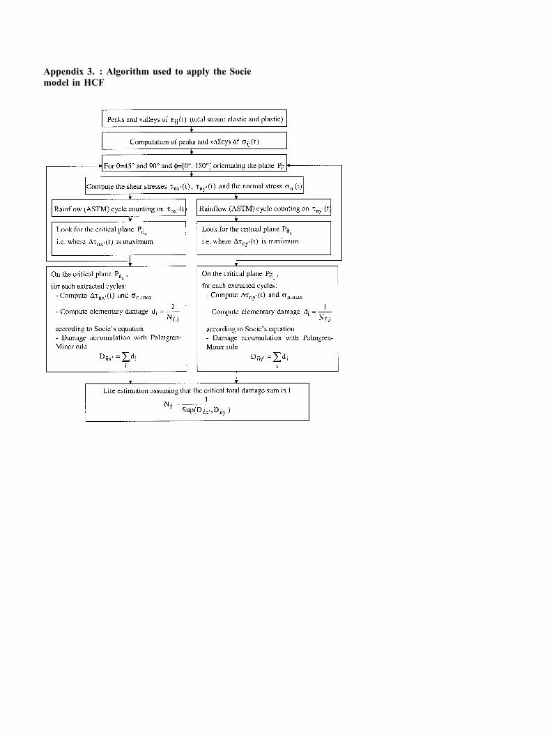
Appendix 3. : Algorithm used to apply the Sociemodel in HCF

Appendix 4. : Algorithm used to apply the Wang-Brown model

Appendix 5. : Algorithm used to apply the Morelfatigue life calculation method

Appendix 6. : Scheme showing differences andsimilarities between the calculation algorithmsapplied to fatigue life determination both in timeand frequency domain

References

[1] Łagoda T, Macha E. Generalization of energy multiaxial cyclicfatigue criteria to random loadings. In: Kalluri S, Bonacuse PJ,editors. Multiaxial fatigue and deformation: testing and predic-tion, ASTM STP 1387. West Conshohocken, PA: AmericanSociety for Testing and Materials; 2000. p. 173–90.

[2] Łagoda T, Macha E, Be�dkowski W. A critical plane approachbased on energy concepts: Application to biaxial random tension-compression high-cycle fatigue regime. Int J Fatigue1999;21(5):431–43.

[3] Łagoda T. Energy models for fatigue life estimation under ran-dom loading—part I—the model elaboration. Int J Fatigue2001;23(6):467–80.

[4] Łagoda T. Energy models for fatigue life estimation under ran-dom loading—part II—verif cation of the model. Int J Fatigue2001;23(6):481–9.

[5] Bannantine JA, Socie D. A variable amplitude multiaxial fatiguelife prediction method. In: Kussmaul K, McDiarmid D, Socie D,editors. Fatigue under biaxial and multiaxial loading, ESIS 10.London: MEP; 1991. p. 35–51.

[6] Fatemi A, Socie DF. A critical plane approach to multiaxialfatigue damage including out-of-phase loading. Fatigue FractEngng Mater Struct 1988;11(3):149–65.

[7] Socie D. Critical plane approaches for multiaxial fatigue damageassessment. In: McDowell DL, Ellis R, editors. Advances inmultiaxial fatigue, ASTM STP 1191. Philadelphia, PA: ASTM;1993. p. 7–36.

[8] Wang CH, Brown MW. A path-independent parameter for fatigueunder proportional and non-proportional loading. Fatigue FractEngng Mater Struct 1993;16(12):1285–98.

[9] Wang CH, Brown MW. Multiaxial random load fatigue: life pre-diction techniques and experiments. In: Pineau A, Cailletaud G,Lindley TC, editors. Multiaxial fatigue and design, ESIS 21. Lon-don: MEP; 1996. p. 513–27.

[10] Morel F. A critical plane approach for life prediction of high

cycle fatigue under multiaxial variable amplitude loading. Int JFatigue 2000;22:101–19.

[11] Morel F. Fatigue multiaxiale sous chargement d’amplitude vari-able. PhD thesis, University of Poitiers, France, 1996.

[12] Morel F. A fatigue life prediction method based on a mesoscopicapproach in constant amplitude multiaxial loading. Fatigue FractEngng Mater Struct 1998;21:241–56.

[13] ASTM Standard practices for cycle fatigue counting in fatigueanalysis, Designation E 1049-85, vol. 03.01 of metal test methodsand analytical procedure. Philadelphia, PA: ASTM; 1985. p.836–48.

[14] Bannantine JA, Socie DF. Multiaxial fatigue life estimation tech-niques. In: Mitchell M, Landgraf R, editors. Advances in fatiguelifetime prediction techniques, ASTM STP 1122. Philadelphia,PA: ASTM; 1992. p. 249–75.

[15] Sonsino CM, Kaufman H, Grubisic V. Transferability of materialdata for the example of a randomly loaded truck stub axle, SAETech. paper series, 970708, 1997. p. 1–22.

[16] Fatemi A, Kurath P. Multiaxial fatigue life predictions under theinf uence of mean-stresses. J Engng Mater Tech Trans ASME1988;110:380–8.

[17] Chaudhury GK, Dover WD. Fatigue analysis of offshore plat-forms subject to sea wave loadings. Int J Fatigue 1985;7(1):13–9.

[18] Liu HJ, Hu SR. Fatigue under non normal random stresses usingMonte - Carlo method. In: Ritchie RO, Starke Jr EA, editors.FATIGUE ‘87. EMAS; 1987. p. 143–9.

[19] Lachowicz C, Łagoda T, Macha E. Comparison of analytical andalgorithmical methods for life time estimation of 10HNAP steelunder random loadings, In: Lutjering G, Nowack H, editors.Fatigue 96, vol. I, Berlin, 1996. p. 595–600.

[20] MSC/FATIGUE user’s guide, vibration fatigue theory, pp. 644–8.[21] Lachowicz C, Łagoda T, Macha E, Dragon A, Petit J. Selections

of algorithms for fatigue life calculation of elements made of10HNAP steel under uniaxial random loadings. Studia Geotech-nika et Mechanica 1996;XVIII(1-2):19–43.

[22] Banvillet A. Prevision de duree de vie en fatigue multiaxiale souschargements reels: vers des essais acceleres. PhD thesis,ENSAM, Centre de Bordeaux, 2001. p. 201.