Fairness Assurance through TXOP Tuning in IEEE 802.11p...

Communications and Network, 2013, 5, 69-83 http://dx.doi.org/10.4236/cn.2013.51007 Published Online February 2013 (http://www.scirp.org/journal/cn)

Fairness Assurance through TXOP Tuning in IEEE 802.11p Vehicle-to-Infrastructure Networks for Drive-Thru

Internet Applications*

Vettath Pathayapurayil Harigovindan, Anchare V. Babu, Lillykutty Jacob Department of Electronics and Communication Engineering, National Institute of Technology Calicut, Kozhikode, India

Email: [email protected], [email protected], [email protected]

Received December 21, 2012; revised January 22, 2013; accepted February 20, 2013

ABSTRACT

This paper addresses an unfairness problem that exists among vehicles of distinct velocities in IEEE 802.11p based ve-hicle-to-infrastructure (V2I) networks used for drive-thru Internet applications. The standard IEEE 802.11p does not take into account, the residence time of vehicles within the coverage of each road side unit (RSU), for granting channel access. Due to this, a vehicle moving with higher velocity has less chance to communicate with the RSU, as compared to vehicles with lower velocity, due to its shorter residence time in the coverage area of RSU. Accordingly, the data transfer performance of a higher velocity vehicle gets degraded significantly, as compared to that of the vehicle with lower velocity, resulting in unfairness among them. In this paper, our aim is to resolve this unfairness problem by as-signing the transmission opportunity (TXOP) limits to vehicles according to their mean velocities. Using an analytical model, we prove that tuning TXOP limit proportional to mean velocity can ensure fairness among vehicles belonging to distinct classes of mean velocities, in the sense of equal chance of communicating with RSU. Analytical results are validated using extensive simulations. Keywords: Fairness; IEEE 802.11p; Residence Time; TXOP; Vehicle-to-Infrastructure Networks

1. Introduction

Vehicular Ad-hoc Networks (VANETs) are highly mo-bile wireless ad hoc networks envisioned to provide support for road safety, traffic management, and comfort applications by enabling vehicle-to-vehicle (V2V) as well as vehicle-to-infrastructure (V2I) communications [1]. Each vehicle equipped with an On-Board Unit (OBU) can either transmit hop-by-hop to the destination using V2V communication or transmit to the RSU using V2I communication. The Dedicated Short Range Communi-cations (DSRC) has been proposed as the emerging technology that supports vehicular communications. The Federal Communication Commission (FCC) in USA has approved 75 MHz of spectrum between 5850 and 5925 MHz for DSRC to enhance safety and productivity of the transportation systems. The Task Group known as IEEE 802.11p has been formed in 2004 for developing an amendment to the 802.11 standard to include vehicular environments, based on the ASTM E2213-02 specifica-tions [2]. This amendment is currently known as IEEE 802.11p [3].The IEEE working group 1609 has been

formed to specify additional layers of the protocol stack. The combination of IEEE 802.11p and the IEEE 1609 protocol suite is designated as WAVE (Wireless Access in Vehicular Environments).The overall WAVE archi-tecture includes IEEE standards 1609.1 to 1609.4 (for resource management, security architecture, networking services, and multichannel operation, respectively), and IEEE 802.11p (for MAC and PHY) [1].

Besides the delivery of infotainment services, the role of typical V2I systems will include the provisioning of safety related, real-time, local, and situation-based ser-vices, such as speed limit information, safe distance warning, lane keeping support, intersection safety, traffic jam warning, and accident warning. All these services aim to prevent accidents by providing timely information directly to the car and/or to the driver. The goal of drive- thru Internet [4,5] is to provide hot spots along the road—within a city, or on a highway. The main technical challenges for communication in V2I and V2V networks are the very high mobility of the nodes, highly dynamic topology, high variability in node density, and very short duration of communication.

*Some part of this work was presented at 2012 ACM International Conference on Advances in Computing, Communications and Infor-matics (ICACCI-2012), Chennai, India.

The IEEE 802.11p uses an enhanced distributed channel access (EDCA) medium access control (MAC)

Copyright © 2013 SciRes. CN

V. P. HARIGOVINDAN ET AL. 70

sub-layer protocol based on distributed coordination function (DCF) [3]. DCF ensures equal channel access probabilities for the contending nodes; but cannot provide service differentiation if the nodes carry frames with different priority levels [6]. The EDCA mechanism [7] assigns four different priority classes for incoming packets at each node which are called Access Categories (AC). Each AC has its own channel access function when compared with the legacy DCF in which all packets exploit the same access function to acquire the channel. The EDCA mechanism defines the channel access parameters such as the Arbitration Inter frame Space (AIFS), the minimum Contention Window

min , the maximum CW max and the Trans- mission Opportunity (TXOP) per each AC in order to provide service differentiation [7]. During an EDCA TXOP, a node is allowed to transmit multiple Protocol Data Units (PDUs) from the same AC with a SIFS time gap between an ACK and the subsequent frame. Prior works [8-10] have proved that TXOP is an efficient techniques for providing service differentiation in 802.11 WLANs.

CW CW

CW

The problem of unfairness due to vehicles having dif-ferent velocities has been analyzed in [11,12] for the V2I communication scenario shown in Figure 1, in which vehicles try to get connected to intermittent and serial RSUs along the highway. Vehicles having different ve-locities have different resident times in the coverage area of an RSU. However, DCF protocol does not take into consideration, the resident time of vehicles for granting channel access. Assuming a saturated network, if all the vehicles in the network use the same MAC parameters, DCF protocol provides equal transmission opportunity for all of them [6]. When vehicles have different veloci-ties, they do not have similar chances of communication with RSU due to the different resident times and, there-fore, a fairness problem exists. A fast moving vehicle has less chance to communicate with its RSU and conse-quently reduced data throughput performance as com-pared to a slow moving vehicle. This problem occurs for each area covered by an RSU. Therefore, the amount of data transferred at each area (useful for next areas) is not equal. In this paper, our aim is to resolve this unfairness problem by adjusting the TXOP of each vehicle accord-ing to its speed. In this way, the amount of successfully transmitted data of all vehicles is made equal regardless of their velocities, while residing in the coverage area of an RSU. Using Jain’s fairness index, we show how fair-ness in the sense of equal chance of communicating with RSU can be achieved by appropriate tuning of TXOP among vehicles of distinct mean velocity classes in the network. The impact of these choices on data throughput performance is also presented.

The rest of this paper is organized as follows. Section

2 presents a brief account of related work. In Section 3, we present the system model for V2I network and provide the expression for computing the data transferred. In Section 4, we discuss how bit-based fairness can be ensured by tuning TXOP limit according to mean velocity of vehicle. The analytical and simulation results are presented in Section 5. The paper is concluded in Section 6.

2. Related Work

Several attempts have been made to analyze and evaluate the performance of IEEE 802.11p standard for vehicular networks in terms of throughput and other related measures [11-23]. In [13,14], authors propose analytical models to evaluate the performance and the reliability of IEEE 802.11a-based V2V safety-related broadcast services in DSRC system on highway. Au- thors of [15] propose a simple but accurate analytical model to evaluate the throughput performance of DCF in the high speed V2I communications. They show that with node velocity increasing, throughput of DCF decreases monotonically due to mismatch between CW and mobility. In [16], the same authors used a 3D markov chain to evaluate the throughput of DCF in the drive-thru Internet scenario. In [17], authors propose an analytic model to evaluate the DSRC-based inter-vehicle communication. The impacts of the channel access parameters such as AIFS and CW are investigated. Analytical model for DSRC network that uses the IEEE 802.11 DCF MAC protocol is developed in [18]. In [19,20], authors derive analytical models to characterize the average and the distribution of the number of bytes downloaded by a vehicle by the end of its sojourn through an AP’s coverage range, in the presence of contention by other vehicles. Authors of [21] propose a new vehicular channel access scheme to compromise the trade-off between system throughput and throughput fairness in V2I networks. In [23], authors conduct a study on association control over the drive-thru Internet scenario for a V2I network. The overall aim is to improve the throughput and fairness for all the users.

The problem of unfairness due to vehicles having different velocities has been explained for a V2I scenario in [11,12] and for a V2V scenario in [22]. Authors of [11] present an analysis, in which the network that spans the coverage area of RSU is modeled as an M/G/1 queue. Using this model, they obtain an expression for the saturation throughput. They also approximate the number of packets transmitted by a node during its residence time by a Poisson random variable. Using these approxi- mations and results from Bianchi’s analysis [6], they derive an approximation for the optimal min for fair access. In [12], optimal minCW required for ensuring fairness, in the sense of equal chance of communicating with RSU, among competing vehicles of different mean



velocities in the network, are evaluated. In [23], authors propose two dynamic CW based mechanisms to alleviate the performance degradation caused by vehicle mobility in V2V networks. But the paper does not describe the exact procedure for the selection of optimal CW value to achieve the objectives.

The effectiveness of TXOP based service differentia-tion has been extensively analyzed and evaluated in WLAN (e.g., [8-10]). In [8], the authors propose an ana-lytical model to evaluate the impact of TXOP limits on the throughput of different access categories in WLANs. In [9], the authors incorporate the TXOP scheme into the infrastructure-based WLANs for throughput improve-ment. In [10], also authors propose TXOP adaptation to improve the performance of WLANs. In this paper, we study the impact of tuning TXOP on the data throughput performance of a V2I network in which vehicles are classified according to their mean velocities. The main objective is to resolve the unfairness among vehicles due to their distinct velocities.

3. Analytical Model for Data Transferred

The system model employed for the analysis includes models for highway and vehicle mobility, and is similar to that of [12]. Consider the V2I scenario, as shown in Figure 1, with vehicles connecting to intermittent and serial RSUs along the highway. Assume that each vehicle has always a frame ready for transmission (i.e.,saturation assumption). Also, we assume perfect channel conditions (i.e., no transmission errors), and neglect the effect of hidden and exposed terminals. Such assumptions are generally used for computing MAC layer throughput of wireless networks [6,12,15,16].

In application specific networks, like V2I, service providers will not pursue full coverage because of the high deployment and the maintenance costs, which in turn, results in non-coverage areas in the network. Even if they provide full coverage with contiguous areas covered by different RSUs and hand offs between them, some emergency information (e.g., status of traffic load, probable crashes occurred in the next road, etc.) must be communicated at each area. Since we are interested in the amount of information at each area (useful for next area) communicated to different vehicles, we focus on one coverage area (zone 1) and outside region (zone 0) only. Unlike [15] in which the system model has multiple zones within the coverage area of an RSU with distinct transmission rates determined by the distances of the nodes from the RSU, our system model has only one zone within the coverage area of an RSU.

We consider the highway to be multi lane, with N lanes, where lane i is used by vehicles with mean speed vi

. Classifying the vehicles according to their mean speed, we have N classes of vehicles, a class vehicle has a mean speed

i

vi . Let be the no of

vehicles belonging to class . The probability density function of iV , the random variable representing class i

ehicle velocity, is assumed to be uniform [14], [24] in the interval

in

i

v mi , , n, max,i iv v with vi

representing the mean and vi

representing the standard deviation. Accordingly, max, = 3i vi

v vi is the maximum

speed and min = 3 v,i vi iv

iV

is the minimum speed. The pdf of is given by

1 1; 3 3

2 3=

0; otherwise

v v i v vi i i ivV i ii

vf v

i

(1)

The residence time of class vehicle in the coverage

area of RSU is a random variable defined as 11, = ;i

i

dT

V

1,i Ni

where 1d is the length of zone 1. The mean sojourn time of class vehicle in the coverage area is calculated as follows [12]:

1, 1

3

1

3

1

1=

1 1= d

2 3

3= ln

2 3 3

ii

v vi i

ii vv v ii i

v vi i

v v vi i i

E T dE V

d vv

d

i

E T

(2)

A class vehicle entering zone 1 resides in the coverage area of the RSU for a mean time duration

1,i

i

before moving out. The mobility of vehicles can then be represented by the zone transitions using a Markov chain model as shown in Figure 2. To facilitate the use of discrete Markov chain model for the throughput analysis, the time that a class node stays in each zone (zone 1 or zone 0), is assumed to be a geometrically distributed random variable with mean

,z i 0,1z . Within a small duration, E T , , class vehicles in zone 1 either move to zone 0 with probability i

1,iE T

, or remain in zone 1 with probability

1,

1iE T

. The limiting probability that a node is in

zone 1 at any time is given by 1

1 0

d

d d 0d

'L

,i j

, where is

the length of zone 0. When a vehicle is within the communication range of RSU, packet transmissions are coordinated by the DCF protocol. The packet length is assumed to be fixed and same for all nodes. Let be the maximum value of back off stage (assumed to be equal for all the nodes), W represent the CW in the


V. P. HARIGOVINDAN ET AL.

yright © SciR CN

72

thj L

CW

Cop 2013 e s.

retry/retransmission for class i and denotes the maximum retry limit in DCF protocol. Further, it is assumed that, vehicles belonging to different mean velocity classes use the same AIFS which is equal to DIFS; but they can be configured to use different values for min and TXOP limit. With these assumptions the conditional frame transmission probability, i that the class vehicle transmits a frame in a time slot, given that the vehicle is in zone 1, given by [12] (see the Equation (3) below).

i

where

'c i , ,c ip p

E T

Wp

1,

c

i

E T

= 1 .

Here ,mini is the minimum CW of class i vehicle, is the conditional collision probability for the class

vehicle; ,c i

i cE T

1,iE T

ip

i

represents the mean collision duration; and is the mean residence time for class vehicle.

The conditional collision probability for the class vehicle ,c i can be expressed in terms of the frame transmission probability as follows [6]:

1

,=1,

= 1 1 1N

n ni lc i i l

l l i

p

p

=1

= 1 1N

nltr l

l

p

(4)

Let tr be the probability that at least one vehicle transmits in a given slot time; clearly,

(5)

The conditional probability ,s i that the transmission from a class vehicle is successful; is given by,

pi

i

1

=1,,

1 1

=

Nn ni l

i i i ll l i

s itr

n

pp

i

(6)

The average successful payload information transmitted for class vehicles that are within the coverage area of RSU is computed as follows [10,12]:

Average pay d info tion f lass vehicle transmitted in as lot time= Meanresidence time for class

erage gth of as lot timei

iloa rma

Av

or c

lenZ i

,s i1,=

1 1tr i

i itr tr s s s c

p p X E

tr

M MAC and Physical header) and an ACK, respectively. Further, SIFS and DIFS represents the short inter frame space and the distributed inter frame space respectively and are defined according to IEEE 802.11p standard. To compute the data transferred according to (7), first of all,

i

Z E Tp p E T p p E T p

(7)

where E Mp

is the average payload length (assumed to be equal for all nodes); tr is the probability that at least one vehicle transmits in a given slot time; ,s i is the probability that a class vehicle transmits and it is successful; i

and ,c i are determined using (3) and (4). Note that (3) and (4) form a system of non linear equations which can be solved using numerical techniques, to get

p

i

pi and

,c i [6,12]. With the knowledge of ip and ,c i , ip Z can be determined using (7) with the help of (4) to (6), (8) and (12). In V2I networks, the number of vehicles on the highway depends on parameters such as vehicle arrival rate, vehicle density, and vehicle speed. The total arrival rate i

X is the number of frames in one TXOP burst of class i vehicle; sp is the probability that a transmission that occur in a time slot is successful; is the duration of a empty time slot; 1,i is the mean sojourn time for class within the coverage of RSU;

E T i

sE T of class vehicles to the RSU can be determined as

i

=i i vik

and c , respectively, represent the mean duration of successful and collision slots. Now assuming RTS/CTS scheme,

E T

sE T (9)

k

and cE T

are computed as follows [10]:

where i is the vehicle density on lane i along the highway segment and vi ,=s s i X i H s sE M

i

E T p T p O

T is the mean vehicle speed (m/sec). According to Greenshield’s model [25], the node density linearly changes with the mean velocity

ik vi as =c R ACKE T T SIFS DIFS

ACKO T T T SIFS T DIFS

TS

T

= 3

(8)

Here , s RTS CTS E M

where RTS and CTST represents the time required to transmit RTS and CTS packets respectively;

T

HT

ACK

and denote the time to transmit the header (including T

= 1vi

i jamfree

k kv

(10)

where jam is the vehicle jam density at which traffic flow comes to a halt,

k

freev

is the free moving velocity,

1' ', ,

' ' '1 1 1'' ' ' ' ' ' ', , , , ,min , , ,

2 1 1 2=

1 2 1 2 1 2 1

L

c i c i

iL L L L LL

c i c i c i c i i c i c i c i

p p

p p W p p p

(3)

,miniW1 2 1p p


i.e., the maximum speed with which vehicle can move, when the vehicle is driving alone on the road (usually taken as the speed limit of the road). The mean number of class nodes, i in the highway segment, is then determined using Little’s theorem as follows [12,15]:

i N

1 01vi

amree

d d

i

1 0= =ii j

v fi

d dN k

v

(11)

The number of class vehicles within the coverage area of RSU is given by

1

1 0

= =i i

dn N k

d d 11vi

jamfree

dv

(12)

4. Ensuring Fairness by TXOP Differentiation

Our objective is to ensure that all competing vehicles in the network achieve same amount of data transferred

regardless of their velocities. Let = ii

i

Zz

n

=1=

N

iin U

= , = 1, 2,3, ,jz z j N

S

be the bits

transferred per vehicle for class and let i

be the total number of vehicles in the network. To ensure fairness, our aim is to achieve the following

(13)

It may be noted that if all the vehicles in the network use the same data rate, (13) results in bit-based fairness.

4.1. Two Classes of Mean Velocities

In the discussion that follows, the subscripts and F correspond to classes of slow and fast vehicles, respectively. Let S denote the number of slow moving vehicles and

n

Fn denote the number of fast moving vehicles. Also, let vS

and vF , respectively, denote

the mean velocities of the slow and fast moving vehicles and let 1,SE T and 1,FE T , respectively, be mean values of their residence times. Further, let ,minS and

,minF be the minimum CW corresponding to the two classes of velocities. Let the conditional frame transmission probabilities of slow and fast nodes be S

WW

and

F , respectively; and the corresponding collision probabilities be ,c S and ,c F . Using (3), p p S and F can be respectively expressed as [6]:

1' ', ,

' ' '1 1 1'' ' ' ' ' ' ',min , , ,min , , ,

2 1 1 2=

1 2 1 1 2 1 2 1 2 1

L

c S c S

SL L L L LL

c S S c S c S S c S c S c S

p p

p p W p p W p p p

, ,c S

(14)

1' ', ,

' ' '1 1 1'' ' ' ' ' ' ', , ,min , , ,min , , ,

2 1 1 2=

1 2 1 1 2 1 2 1 2 1

L

c F c F

FL L L L LL

c F c F F c F c F F c F c F c F

p p

p p W p p W p p p

(15)

where

', ,= 1c S cp p

E T

1,

c

S

E T

S

and

'c F

, = 1

, ,= 1E T

p pE T

p ,c Fp

1n

1,

c

F

1S

c F

,c S

n

.

Further, the collision probabilities and are expressed as:

1 Fc S

, = 1c F

S

1 S

p

= 1 1 1n nS

F

n

S

p

p

11

nF

F (16)

Recall that tr is the probability that there is at least one transmission in the given time slot, and let ,tr S and

,tr F be the corresponding probabilities for slow and fast nodes, respectively. These probabilites are calculated

pp

as follows:

Ftr S Fp

(17)

The successful transmission probabilities, as defined in (6), for the two classes are:

1

,

1 1=

n nS FS S S F

s Str

np

p

1

,

1 1=

nn SFF F F S

s Ftr

np

p

(18)

The amount of bits transferred, for slow and fast moving vehicles are given by,

,=1 1

tr s S S

s c

p p X E MZ

p p E T

1,

Str tr s s tr

S

p p p E T

E T

,1,=

1 1tr s F F

F Ftr tr s s tr s c

p p X E MZ E T

p p p E T p p E T (19)



Here SX and FX respectevely represents the

number of frames in the TXOP burst of slow and fast vehicles respectively. We use the following Jain’s Fairness Index [26], in evaluating the fairness of channel access:

2

=1

2

=1

=

U

ii

U

ii

y

U y

Uy

1

F (20)

where is the total number of vehicles in the network, and i ’s are the individual vehicle share. It may be noted that F = .y y i and equality holds iff i An approximate ratio of bits transferred per vehicle for slow and fast vehicles can be obtained using (16)-(19) as follows. Assume that min of all classes of vehicles are the same and differentiation is in terms of TXOP alone. From (18), we have

CW

,

1 1

1

1

c S S

c F F

n nS

,

= 1

= 1 FS F

W W , 1

p

p .

Assume ,min ,minS F and S F, 1 so that

, ,c S c F . Utilizing (19), we have the following approximation for the ratio of bits transferred for slow and fast vehicles. Then the ratio of data transferred per node for slow and fast vehicles is given by

p p

1,

1,

S SS

F F F

X E T

X E T

=S S

F F

z Z n

z Z n (21)

Since 1F when S F , the optimal TXOP limit for the fast vehicle to achieve desired fairness objective can be obtained as follows:

=z z

1,

1,

S

F S

F

E T

E T

n

X X (22)

When optimal TXOP is chosen according to (21), the ratio of bits transferred per node for slow and fast vehicles become equal to unity, thus resulting in bit based fairness. Under default TXOP setting in which TXOP values are selected as equal, for all vehicles irrespective of their velocities, the above ratio is equal to the ratio of residence times of slow and fast vehicles.

4.2. Three Classes of Mean Velocities

In this section, we extend our analysis to a V2I network in which there are three classes of mean velocities: slow (S), medium (M) and fast (F). Let S , Mn , Fn , respectively, denote the number of vehicles corresponding to the three categories. vS

, vM and vF

, respectively, be their mean velocities; and , 1,SE T 1,ME T

1,FE T

and 1, > >E T E T E T, respectively, be their mean residence time.

Clearly, 1, 1,S M F . Further, let S ,

M and F be the conditional frame transmission probabilities and let ,c S , ,c M and ,c F be the frame collision probabilities of slow, medium and fast vehicles, respectively.

p p p

To ensure fairness, the TXOP limits of medium and fast vehicles are to be increased to improve their opportunity for channel access. Keeping the TXOP of slowest vehicle constant at default value (unity), the optimal TXOP pair ,M FX X

1 required to achieve

F is determined. The fairness index F becomes equal to unity when S M F , where i = =z z z z = , ,i S M F

CW

represent the bits transferred per node for slow, medium and fast nodes respectively. Assuming that

min of all vehicles are same, expressions similar to (20) can be obtained as

1,

1,

S SS

F F F

X E Tz

z X E T

1,

1,

S SS

M M M

X E Tz

z X E T

(23)

Hence approximate expressions for optimal TXOP limits for medium and fast vehicles can be obtained as follows:

1,

1,

S

M S

M

E TX X

E T

1,

1,

S

F S

F

E TX X

E T

(24)

Note that FX required to achieve bit based fairness in a network with three classes of mean velocities is same as that of two classes case. Also, MX required to achieve bit based fairness in network with three classes of mean velocities is same as that required in a network two velocity classes, where the mean velocities are vM

and vS

. Thus the optimal value of TXOP required to achieve bit based fairness in a network with two velocity classes, hold for network with three mean velocity classes as well. For a V2I network with N number of mean velocity classes, the results of (23) can be extended for all the higher velocity classes, provided we consider the slowest vehicle to be the reference node.

4.3. Joint Adaptation of TXOP and minCW

CWIn this section, we consider joint adaptation of the

min and TXOP among vehicles belonging to distinct mean velocity classes to ensure the desired fairness objective. We consider the case with two mean velocity



classes. Let ,minS and ,minFW be the minimum CW of slow and fast vehicles. Assume ,m , ,minF , so that S F

W

, 1inSW 1W

. Also, let SX and FX be the TXOP burst size corresponding to these two velocity classes. An approximate expression of ratio of data transferred per node for slow and fast vehicles can be obtained by using (16)-(19) as follows:

1

1

1,

1,

nSS

nFF

S S

F F

S

F

n

n X

n X

X E T

E T

1,

1,

1,

1,

1 1

1 1

nFF S SS

nSF S F F

SS

FF

S

F

X E T

X E T

E T

E T

n

1

1

S S

F F

S

F

S S

F F

n

n X

Z

Z

(25)

Then using (14), (15) and assuming the retry limit to be infinite, the following approximation is valid [12]:

,min

,min

F

F S

W

W=S

.

Then ratio of the bits transferred,

S

F

Z

Z is given by

,min 1,

,min 1,

S F S S

F S F F

n W X E T

n W X E T

S

F

Z

Z (26)

The ratio of the bits transferred per node is given by

,m

,m

=S S S

F F F

z Z n

z Z n in 1,

in 1,

F S S

S F F

W X E T

W X E T

1 =S Fz zW

(27)

To provide fairness in terms of data transferred, we have to ensure that F which makes . To ensure this, we consider combined tuning of ,minF and

FX of fast vehicles according to the following relation:

,min 1,S F S FX W E T X ,min 1,S FW E T

1,,min

1,

F

F S S

E T

E T

,minF SW W

X X (28)

We can select default values for ,minS and SW X ; and compute ,minF and W FX , so as to satisfy (27), thus we ensure the ratio of bits transferred for slow and fast vehicles equal to unity.

5. Analytical and Simulation Results

In this section, we present the analytical and simulation results. The analytical results correspond to the mathematical model presented in the previous section

and are obtained using MATLAB. To validate the analytical results, we simulate a IEEE 802.11p based V2I network using an event driven custom simulation program,written in C++ programming language. It may be noted that the MAC layer of IEEE 802.11p is based on EDCA and physical layer is based on IEEE 802.11a. A drive-thru Internet scenario as shown in the Figure 1 is simulated, in which RSU is deployed along the road and vehicles passing through compete for communication. The whole road length is divided into two segments with one zone in the coverage area of RSU and other zone representing the region outside the coverage of RSU (we set 1 and 0250 md 50 md ). We simulate the road segment as composed of as many lanes as the number of classes of vehicles; e.g., for the case of three classes, a three lane road segment is simulated. Vehicle of class arrive according to a Poission process with rate i

i veh/sec. Lane i is used

by vehicles belonging to class of velocity iv . The probability distribution for is assumed to be uniform between the interval min, max,i i with vi

i

iv,v v

representing the mean vehicle speed and vi , the

standard deviation. We consider traffic jam density

jam 80k veh/km/lane and the free flow speed is selected as free 160v km/hr [25]. The system parameters used for simulation as well as for finding the numerical results from analysis are given in Table 1. All reported simulation results are averages over multiple 100 sec simulations.

The number of vehicles corresponding to different classes of mean velocities, within the coverage area of RSU, are obtained using (12) with jam : 80 veh/km/lane. Table 2 lists the number of slow and fast vehicles in a network with two classes of mean velocities and Table 3 lists the number of vehicles in a network with three classes of mean velocities for different choices of mean velocities. These results are later used to investigate the data throughput performance of V2I networks. Table 4 shows the TXOP values required to ensure fairness, for a network in which the vehicles belong to two classes of mean velocities, and Table 5 shows corresponding results for a network that consist of vehicles categorized in to three classes of mean velocities.

k

7LTo find the data transferred, the MAC parameters for

slow and fast vehicles are kept the same: , ,

,minS , ,minF

' =5L=32W 32W . The default TXOP values are

selected to be equal to unity. Further, we select vS =

3 0 / 4 0 / 6 0 k m / h r , 120vF 80jamk k m / h r ,

veh/km/lane, v vS F5 160v km/hr and free

km/hr. The number of vehicles corresponding to these specifications are listed in Table 2. We evaluate the fairness index, according to (20) for default TXOP as well as optimal TXOP values, and the results are shown in Table 6. It can be observed that with optimal TXOP



Table 1. System parameters.

Parameter Value

Packet payload 8184 bits @ 6 Mb/s

MAC header 256 bits @ 6 Mb/s

PHY header 192 bits @ 3 Mb/s

ACK 112 bits PHY header @ 3 Mb/s

2 μs

13μs

32 μs

58 μs

Channel Bit Rate 6 Mb/s

Propagation Delay

Slot Time

SIFS

DIFS

Table 2. Network size: two classes of mean velocities.

Mean velocities 80jamk

,v vS F (km/hr) veh/km/lane

Sn Fn

30, 120 16 5

40, 120 15 5

60, 120 12 5

120, 120 5 5

Table 3. Network size: three classes of mean velocities.


, ,v v vS M F (km/hr) veh/km/lane

Sn Mn Fn

40, 80, 120 15 10 5

50, 100, 150 13 7 1

Table 4. TXOP to ensure fairness (two classes).


,v vS F (km/hr) veh/km/lane

TXOP of TXOP of

Slow class Fast class

30, 120 1 4

40, 120 1 3

60, 120 1 2

120, 120 1 1

Table 5. TXOP to ensure fairness (three classes).

80jamk Mean velocities

, ,v v vS M F (km/hr) veh/km/lane

TXOP of TXOP of TXOP of

Slow class Medium class Fast class

40, 80, 120 1 2 3

50, 100, 150 1 2 3

40, 120, 160 1 3 4

settings, the fairness index can be made equal to unity. We find the amount of data transferred for slow and fast vehicles by analysis using (19) as well as by simulation. The results are shown in Table 7. We find that the data transferred for fast vehicles is very low compared to slow vehicles with default TXOP settings. The low data transfer for fast vehicle is caused by the DCF protocol which does not consider residence time of a vehicle for granting channel access. Further, we observe that for default MAC settings, the ratio of data transferred per node for slow and fast vehicles is equal to the ratio of their mean residence times, thus validating our analytical result of (21). When TXOP values are selected according to (21), the amount of data transferred by slow as well as fast vehicles are observed to be equal. However, we observe a slight reduction in the total amount of data transferred (in Table 7) for the optimal case compared to the default case. This is in accordance with the established result on trade off between fairness and efficiency.

In Figure 3 aggregate data transferred in a network with two classes of mean velocities, plotted against the mean velocity of slow vehicle vS

, keeping the mean velocity of fast vehicle as fixed: vF

km/hr. It is observed that the aggregate data transferred decreases as

vS

120

increases. This happens because, as vS increases

the mean residence time reduces, resulting in reduced channel access for slow vehicle as well. Figure 4 shows the ratio of data transferred per node for fast and slow vehicle F s , plotted against the mean velocity of slow vehicle ( vS

z z km/hr). vF

km/hr and vS120

is varied from 30 km/hr to 120 km/hr. In default case, the ratio F s is equal to unity when vS

z z is 120 km/hr, and decreases as vS

decreases. This happens because, as vS

decreases, its residence time within RSU’s coverage increases and hence S increases. When the optimal TXOP settings are used, both the slow and fast vehicles get the same chances of communication with the RSU, and hence the ratio of data transferred is almost equal to unity irrespective of

z

vS .




77

Table 6. Fairness Index with default TXOP and optimal TXOP for two classes ( jam vS

k = 80 veh/km/lane, = vF = 5

km/hr).

Fairness index Velocity of vehicles ,v vS F

(km/hr) TXOP settings

Analytical Simulation

TXOP(S) = 1 Default

TXOP(F) = 1 0.8686 0.8866

TXOP(S) = 1 30, 120

Optimal TXOP(F) = 4

1.0000 0.9999

TXOP(S) = 1 Default

TXOP(F) = 1 0.8929 0.9009

TXOP(S) = 1 40, 120

Optimal TXOP(F) =3

1.0000 0.9999

60, 120 Default TXOP(S) = 1

TXOP(F) = 1 0.9334 0.9367

Optimal TXOP(S) = 1

TXOP(F) = 2 1.0000 0.9999

Table 7. Data transferred (individual and aggregate) with default and optimal TXOP values for two classes ( jamk

vSσ vF

σ

= 80

veh/km/lane, = = 5 km/hr).

Slow vehicle (Mb) Fast vehicle (Mb) Total (Mb) Mean velocity of vehicles (km/hr)

TXOP Settings Analytical Simulation Analytical Simulation Analytical Simulation

TXOP(S) = 1 Default

TXOP(F) = 1 5.1325 5.1071 1.1581 1.1211 89.0638 87.3191

TXOP(S) = 1 30, 120

Optimal TXOP(F) = 4

3.9248 3.9012 3.9248 3.9098 82.4223 81.9682

TXOP(S) = 1 Default

TXOP(F) = 1 4.3997 4.3321 1.3332 1.3087 72.6615 71.525

TXOP(S) = 1 40, 120

Optimal TXOP(F) = 3

3.4307 3.3784 3.4307 3.3812 68.6158 67.582

TXOP(S) = 1 Default

TXOP(F) = 1 3.6241 3.6088 1.812 1.7899 52.5497 52.2551

TXOP(S) = 1 60, 120

Optimal TXOP(F) = 2

3.0167 3.0082 3.0167 3.0091 51.2844 51.1439

5.1. Three Classes of Vehicles

To find the data transferred for a network with three classes of mean velocities, we set veh/ km/lane, free km/hr and v v vS M F

80jamk 160v 5 1

km/hr. The number of slow/medium/fast vehicles corresponding to these traffic parameters are listed in

Table 3. The optimal TXOP values according to (23) are given in Table 5. The fairness index calculated with default and optimal TXOP limits are shown in Table 8. With optimal TXOP, it is observed that F can be achieved. With these optimal TXOP values, we evaluate the aggregate data transferred by slow, medium and fast


Table 8. Fairness Index with default and optimal TXOP values for three classes ( jamk vM

σ v = 80 veh/km/lane, = = vSσ

Fσ

= 5 km/hr).

Fairness index Mean velocity of vehicles , ,v v vS M F

(km/hr) TXOP settings Analytical Simulation

TXOP(S) = 1

TXOP(M) = 1 Default

TXOP(F) = 1

0.8666 0.8759

TXOP(S) = 1

TXOP(M) = 2

40, 80, 120

Optimal

TXOP(F) = 3

1.0000 0.9999

TXOP(S) = 1 Default

TXOP(M) = 1

TXOP(F) = 1

0.9079 0.9109

TXOP(S) = 1

50, 100, 150

Optimal TXOP(M) = 2

TXOP(F) = 3

1.0000 0.9999

INTERNET

RSURSU

Zone 1 Zone 0 Zone 1

6 Mbps 6 Mbps

6 Mbps

6 Mbps

Wireless ConnectionWired ConnectionRSU radio coverage Moving Direction of Vehicles

Figure 1. Vehicle to infrastructure scenario.



Zone 0

Zone 1

Figure 2. Markov chain model for zone transitions.

30 35 40 45 50 55 6020

30

40

50

60

70

80

90

100

Mean velocity of slow vehicle, μv

S

Agg

rega

te d

ata

tran

sfer

red,

Z (

Mb)

→

(km/hr) →

Optimal TXOP (analysis)Optimal TXOP (simulation)Default TXOP (analysis)Default TXOP (simulation)

Figure 3. Aggregate data transferred vs mean velocity of slow station( vF

μ = 120 km/hr and jam vSσ vk = 80, =

Fσ

= 5 km/hr).

Figure 4. Ratio of data transferred per node vs velocity of slow vehicle with default scheme and TXOP tuning (

vehicles. We repeat this calculation for the default TXOP values as well. Both the analytical and simulation results are shown in Table 9. For the default selection of TXOP limits, we find that the amount of data transferred by fast and medium velocity vehicles are very less compared to that of the slow vehicle. With optimal TXOP values, all the vehicles in the network transfer almost equal amount of data, irrespective of their mean velocities; thus ensuring fairness.

5.2. Impact of Standard Deviation of Vehicle Speed

vFμ =

120 km/hr, = = 5 km/hr). vSσ vF

σ

In this section, we describe the impact of standard deviation of vehicle speed on the data throughput performance of V2I network, considering vehicles belonging to two classes of mean velocities. Figure 5 shows the impact of standard deviation of vehicle speed corresponding to slow moving vehicle vS

, on the optimal TXOP limit *

FX of the fast vehicle. We keep the mean velocity of the slow and fast vehicles as follows: 60 80vS

km/hr and vF km/hr.

Further, the standard deviation of the fast vehicle is kept equal to vF

120

5 *F km/hr. For lower values of vS

, X remains invariant with respect to vS

. However, when

vS

*F becomes greater than 10 km/hr, X increases

significantly for the case with vS 60

E T km/hr. This is

due to the increase in mean residence time 1,S of slow vehicle arising out of increase in vS

as predicted by (2).

In Figure 6, we plot the fairness index against vS ,

for the default and optimal TXOP values. We keep the mean velocities of both class of vehicles to be fixed (i.e.,

vS 60 km/hr, vF

km/hr) and fix the standard deviation of fast vehicle as vF

120 5

1X X

km/hr. We find the amount of data transferred for each class of vehicle and evaluate the fairness index. For the default setting, we select S F

vS

. It is observed that, for the default TXOP settings, the fairness index degrades significantly as increases. This happens because with increase of vS

, the mean residence time of slow velocity vehicle 1,SE T increases in accordance (2), assuming that mean velocity vS

is constant. Ac- cordingly, the amount of data transferred by a slow vehicle gets improved; which results in the degradation of fairness index. It is observed that with optimal TXOP values, the fairness index is insensitive to vS

variations and is always equal to unity.

Figure 7 shows the impact of standard deviation of vehicle speed corresponding to slow moving vehicle on the ratio of data transferred per node for fast and slow vehicle F s . The behavior of this plots can be explained in the same way as explained for the fairness plots of Figure 6.

z z



Table 9. Data transferred (individual and aggregate) with default and optimal TXOP values for three classes ( jamk

vMσ v

= 80

veh/km/lane, = = vSσ

Fσ = 5 km/hr).

Slow vehicle (Mb) Medium vehicle (Mb) Fast vehicle (Mb) Total (Mb) Mean velocity of vehicles

(km/hr) TXOP Settings

Analytical Simulation Analytical Simulation Analytical Simulation Analytical Simulation

TXOP(S) = 1

TXOP(M) = 1 Default

TXOP(F) = 1

3.0267 3.0187 1.5123 1.4956 1.0089 1.0068 65.5794 62.1643

TXOP(S) = 1

TXOP(M) = 2

40, 80, 120

Optimal

TXOP(F) = 3

2.265 2.1984 2.265 2.1885 2.265 2.1879 67.9502 65.8005

TXOP(S) = 1

TXOP(M) = 1 Default

TXOP(F) = 1

3.4995 3.4257 1.7497 1.6874 1.1665 1.1458 58.9086 57.4917

TXOP(S) = 1

TXOP(M) = 2

50, 100, 150

Optimal

TXOP(F) = 3

2.7791 2.6984 2.7791 2.6996 2.7791 2.6989 58.9086 56.6753

0 5 10 15 20 25 300.5

1

1.5

2

2.5

3

Standard deviation of slow vehicle velocity, σ

Optim

al T

XO

P o

f fa

st v

ehic

le, X F

vs (km/hr) →

* →

μv

= 80,μv

= 120 (analytical)S F

μv

S

= 80,μv

F

= 120 (simulation)

μv

S

= 60,μv

F

= 120(analytical)

μv

S

= 60,μv

F

= 120 (simulation)

Figure 5. TXOP of fast vehicle vs standard deviation of slow vehicle speed ( σ = 5 km/hr). vF

minCW

CW

CW

minCW

jamk

5.3. Combined Tuning of TXOP and

Next we consider combined tuning of TXOP and min . Table 10 lists the values of TXOP and min required for satisfying the desired fairness objective. With these values, we compute the amount of data transfered. Also, we find the data transferred by choosing the default parameter as well. We then calculate the fairness index and the results are tabulated in Table 11. It is observed that, if the TXOP and min values are selected according to to (28), the fairness index can be made equal to unity. The analytical and simulation results for data transfered are listed in Table 12. It can be observed that, combined tuning of TXOP and CWmin according to (28) results in bit-based fairness, which means that the bits transferred

CW

Table 10. Tuning of txop and .

= 80 veh./km/lane Mean Velocities of

Vehicles ,v vS F

minCW minCW

(km/hr)

TXOP and of Fast class

TXOP and of Slow class

30, 120 TXOP(F) = 2,

F ,minCW ,S minCW = 16 TXOP(S) = 1,

= 32

40, 120 TXOP(F) = 2,

F ,minCW ,S minCW

,

= 22 TXOP(S) = 1,

= 32

60, 120 TXOP(F) = 2,

F minCW ,S minCW

,

= 32 TXOP(S) = 1,

= 32

120, 120 TXOP(F) = 1,

F minCW ,S minCW = 32 TXOP(S) = 1,

= 32

1.02

1

0 5 10 15 20 25 300.86

0.88

0.9

0.92

0.94

0.96

0.98

Standard deviation of slow vehicle velocity, σvs

(km/hr) →

Fai

rnes

s In

dex,

F →

Default TXOP (analysis)Default TXOP (simulation)Optimal TXOP (analysis)Optimal TXOP (simulation)

Figure 6. Fairness index vs standard deviation of slow vehicle speed ( vSμ = 60 km/hr, vF

μ = 120 km/hr, vFσ =

5 km/hr).



Table 11. Fairness index with default and optimal TXOP & values for two classes (minCW jamk = 80 veh/km/lane).

Fairness index Velocity of vehicles ,v vS F minCW

,S minCW

,

(km/hr) TXOP and settings Analytical Simulation

TXOP(S) = 1, = 32 Default

TXOP(F) = 1,

F minCW

,S minCW

,

= 32 0.8686 0.8866

TXOP(S) = 1, = 32 30, 120

Optimal TXOP(F) = 2, F minCW

,S minCW

,

= 16 0.9990 0.9986

TXOP(S) = 1, = 32 Default

TXOP(F) = 1, F minCW

,S minCW

,

= 32 0.8929 0.9009

TXOP(S) = 1, = 32 40, 120

Optimal TXOP(F) = 2, F minCW

,S minCW

,

= 22 0.9998 0.9999

Default TXOP(S) = 1, = 32

TXOP(F) = 1, F minCW

,S minCW

,

= 32 0.9334 0.9367

Optimal TXOP(S) = 1, = 32 60, 120

TXOP(F) = 2, F minCW = 32 0.9999 0.9999

Table 12. Data transferred (individual and aggregate) with default and optimal TXOP values for two classes ( jamk = 80

veh/km/lane).

Slow vehicle (Mb) Fast vehicle (Mb) Total (Mb) Velocity of

vehicles ,S F

(km/hr)

TXOP and CWmin settings Analytical Simulation Analytical Simulation Analytical Simulation

TXOP(S) = 1, CWS,min = 32 Default

TXOP(F) = 1, CWF,min = 32 5.1325 5.1071 1.1581 1.1211 89.0638 87.3191

TXOP(S) = 1, CWS,min = 32 30, 120

Optimal TXOP(F) = 2, CWF,min = 16

3.6358 3.6247 3.7965 3.7814 77.1553 76.9022


TXOP(F) = 1, CWF,min = 32 4.3997 4.3321 1.3332 1.3087 72.6615 71.525

TXOP(S) = 1, CWS,min = 32 40, 120


3.3647 3.3512 3.3749 3.3658 67.345 67.097


TXOP(F) = 1, CWF,min = 32 3.6241 3.6088 1.812 1.7899 52.5497 52.2551

TXOP(S) = 1, CWS,min = 32 60, 120


3.0167 3.0082 3.0167 3.0091 51.2844 51.1439

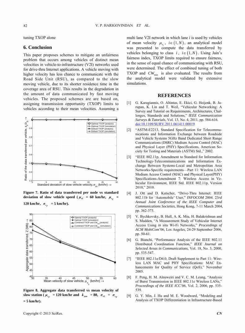
per vehicle are the same for all the classes of vehicles. In Figure 8 aggregate data transferred is plotted against μvS mean velocity of slow vehicle for the two cases con- sidered in this paper: 1) tuning of TXOP alone and 2) combined tuning of TXOP and . It is observed

that the aggregate data reduces as the vS increases

owing to the reduced residence time of slow vehicle in the coverage area of RSU. Further, it is observed that a joint tuning of TXOP and minCW results in reduced aggregate data transferred, as compared to the case of minCW



tuning TXOP alone

6. Conclusion

This paper proposes schemes to mitigate an unfairness problem that occurs among vehicles of distinct mean velocities in vehicle-to-infrastructure (V2I) networks used for drive-thru Internet applications. A vehicle moving with higher velocity has less chance to communicate with the Road Side Unit (RSU), as compared to the slow moving vehicle, due to its shorter residence time in the coverage area of RSU. This results in the degradation in the amount of data communicated by fast moving vehicles. The proposed schemes are are based on, assigning transmission opportunity (TXOP) limits to vehicles according to their mean velocities. Assuming a

0 5 10 15 20 25 300.3

0.4

0.5

0.6

0.7

0.8

0.9

1

Standard deviation of slow vehicle velocity, σ

Rat

io o

f the

dat

a tr

ansf

erre

d pe

r ve

hicl

e, z

F/z

S →

vs (km/hr) →

Optimal TXOP (analysis)Optimal TXOP (simulation)Default TXOP (analysis)Default TXOP (simulation)

Figure 7. Ratio of data transferred per node vs standard deviation of slow vehicle speed ( vSμ = 60 km/hr, vF

μ

vFσ

=

120 km/hr, = 5 km/hr).

30 35 40 45 50 55 6040

45

50

55

60

65

70

75

80

85

90

Mean velocity of slow vehicle, μv

S

(km/hr) →

Agg

rega

te d

ata

tran

sfer

red,

Z (

Mb)

→

Optimal TXOP (analysis)Optimal TXOP (simulation)Combined TXOP and CW

min(analysis)

Combined TXOP and CWmin

(simulation)

Figure 8. Aggregate data transferred vs mean velocity of slow station ( vF

μ = 120 km/hr and jam vSσ vk = 80, = F

σ

= 5 km/hr).

multi lane V2I network in which lane i is used by vehicles of mean velocity vi

, , an analytical model was presented to compute the data transferred by vehicles belonging to class , . Using Jain’s fairness index, TXOP limits required to ensure fairness, in the sense of equal chance of communicating with RSU, were determined. The effect of combined tuning of both TXOP and min is also evaluated. The results from the analytical model were validated by extensive simulations.

1,i N

i 1,i N

CW

REFERENCES [1] G. Karagiannis, O. Altintas, E. Ekici, G. Heijenk, B. Ja-

rupan, K. Lin and T. Weil, “Vehicular Networking: A Survey and Tutorial on Requirements, Architectures, Chal- lenges, Standards and Solutions,” IEEE Communication Surveys & Tutorials, Vol. 13, No. 4, 2011, pp. 584-616. doi:10.1109/SURV.2011.061411.00019

[2] “ASTM-E2213, Standard Specification for Telecommu- nications and Information Exchange between Roadside and Vehicle Systems 5GHz Band Dedicated Short Range Communications (DSRC) Medium Access Control (MAC) and Physical Layer (PHY) Specifications, American So- ciety for Testing and Materials (ASTM) Std.,” 2002.

[3] “IEEE 802.11p, Amendment to Standard for Information Technology-Telecommunications and Information Ex- change Between Systems-Local and Metropolitan Area Networks-Specific requirements—Part 11: Wireless LAN Medium Access Control (MAC) and Physical Layer(PHY) Specifications-Amendment 7: Wireless Access in Ve- hicular Environment, IEEE Std. IEEE 802.11p, Version 2010,” 2010.

[4] J. Ott and D. Kutscher, “Drive-Thru Internet: IEEE 802.11b for ‘Automobile’ User,” INFOCOM 2004. 23rd Annual Joint Conference of the IEEE Computer and Communications Societies, Hong Kong, 7-11 March 2004, pp. 362-373.

[5] V. Bychkovsky, B. Hull, A. K. Miu, H. Balakrishnan and S. Madden, “A Measurement Study of Vehicular Internet Access Using in situ Wi-Fi Networks,” Proceedings of ACM MobiCom’06, Los Angeles, 24-29 September 2006, pp. 50-61.

[6] G. Bianchi, “Performance Analysis of the IEEE 802.11 Distributed Coordination Function,” IEEE Journal on Selected Areas in Communications, Vol. 18, No. 3, 2000, pp. 535-547.

[7] “IEEE 802.11e/D4.0, Draft Supplement to Part 11: Wire- less LAN MAC and PHY Specifications: MAC En- hancements for Quality of Service (QoS),” November 2005.

[8] F. Peng, H. M. Alnuweiri and V. C. M. Leung, “Analysis of Burst Transmission in IEEE 802.11e Wireless LANs,” Proceedings of the IEEE ICC’06, Vol. 2, 2006, pp. 535- 539.

[9] G. Y. Min, J. Hu and M. E. Woodward, “Modeling and Analysis of TXOP Differentiation in Infrastructure-Based


http://dx.doi.org/10.1109/SURV.2011.061411.00019



83

WLANs,” Computer Networks, Vol. 55, No. 11, 2011, 2545-2557. doi:10.1016/j.comnet.2011.04.015

[10] J. Y. Lee, H. Y. Hwangy, J. Shin, and S. Valaee, “Dis- tributed Optimal TXOP Control for Throughput Re- quirements in IEEE 802.11e Wireless LAN,” IEEE Per- sonal Indoor Mobile Radio Communication Symposium (PIMRC), Toronto, 11-14 September 2011, pp. 935-939.

[11] E. Karamad and F. Ashtiani, “A Modified 802.11-Based MAC Scheme to Assure Fair Access for Vehicle-to- Roadside Communications,” Computer Communications, Vol. 31, No. 12, 2008, pp. 2898-2906. doi:10.1016/j.comcom.2008.01.030

[12] V. P. Harigovindan, A. V. Babu and L. Jacob, “Ensuring fair Access in IEEE 802.11p-Based Vehicle-to-Infra- structure Networks,” EURASIP Journal on Wireless Com- munications and Networking, 2012, 168.

[13] X. Chen, H. H. Refai and X. Ma, “On the Enhancements to IEEE 802.11 MAC and their Suitability for Safety- Critical Applications in VANET,” Wireless Communica- tions and Mobile Computing, Vol. 10, No. 9, 2010, pp. 1253-1269. doi:10.1002/wcm.674

[14] X. M. Ma, X. B. Chen and H. H. Refai, “Performance and Reliability of DSRC Vehicular Safety Communication: A Formal Analysis,” EURASIP Journal on Wireless Com- munications and Networking, Vol. 2009, Article ID: 969164, 13 Pages.

[15] T. H. Luan, X. H. Ling and X. M. (Sherman) Shen, “MAC Performance Analysis for Vehicle-to-Infrastruc- ture Communication,” Proceedings of Wireless Commu- nications and Networking Conference (WCNC), Sydney, 18-21 April 2010, pp. 1-6.

[16] T. H. Luan, X. H. Ling and X. M. (Sherman) Shen, “MAC in Motion: Impact of Mobility on the MAC of Drive-Thru Internet,” IEEE Transaction on Mobile Com- puting, Vol. 11, No. 2, 2011, pp. 305-319.

[17] J. H. He, Z. Y. Tang, T. O’Farrell and T. M. Chen, “Per- formance Analysis of DSRC Priority Mechanism for Road Safety Applications in Vehicular Networks,” Wire- less Communications and Mobile Computing, Vol. 11, No.

7, 2011, pp. 980-990. doi:10.1002/wcm.821

[18] M. I. Hassan, H. L. Vu and T. Sakurai, “Performance Analysis of the IEEE 802.11 MAC Protocol for DSRC with and without Retransmissions,” IEEE International Symposium on a World of Wireless Mobile and Multime- diab Networks, Montreal, 14-17 June 2010, pp. 1-8.

[19] W. L. Tan, W. C. Lau and O. Yue, “Modeling Resource Sharing for a Road-Side Access Point Supporting Drive- Thru Internet,” Proceedings of ACM VANET, Beijing, 25 September 2009, pp. 33-42.

[20] W. L. Tan, W. C. Lau, O. Yue and T. H. Hui, “Analytical Models and Performance Evaluation of Drive-Thru Inter- net Systems,” IEEE Journal on Selected Areas in Com- munications, Vol. 29, No. 1, 2011, pp. 207-222.

[21] S.-T. Sheu, Y.-C. Cheng and J.-S. Wu, “A Channel Ac- cess Scheme to Compromise Throughput and Fairness in IEEE 802.11p Multi-Rate/Multi-Channel Wireless Ve- hicular Networks,” IEEE 71st Vehicular Technology Conference, Taipei, 16-19 May 2010, pp. 1-5.

[22] W. Alasmary and W. Zhuang, “Mobility Impact in IEEE 802.11p Infrastructure Less Vehicular Networks,” Ad Hoc Networks, Vol. 10. No. 2, 2010, pp. 222-230. doi:10.1016/j.adhoc.2010.06.006

[23] L. Xie, Q. Li, W. Mao, J. Wu and D. Chen, “Achieving Efficiency and Fairness for Association Control in Ve- hicular Networks,” 17th IEEE International Conference on Network Protocols, 13-16 October 2009, Princeton, pp. 324-333.

[24] H. Wu, R. M. Fujimoto, G. F. Riley and M. Hunter, “Spa- tial Propagation of Information in Vehicular Networks,” IEEE Transactions on Vehicular Technology, Vol. 58, No. 1, 2009, pp. 420-431. doi:10.1109/TVT.2008.923689

[25] R. P. Roess, E. S. Prassas and W. R. Mcshane, “Traffic Engineering,” 3rd Edition, Pearson Prentice Hall, Upper Saddle River, 2004.

[26] R. Jain, W. Hawe and D. Chiu, “A Quantitative Measure of Fairness and Discrimination for Resource Allocation in Shared Computer Systems,” DEC Research Report TR- 301, September 1984.

http://dx.doi.org/10.1016/j.comcom.2008.01.030

http://dx.doi.org/10.1002/wcm.674

http://dx.doi.org/10.1016/j.adhoc.2010.06.006

http://dx.doi.org/10.1109/TVT.2008.923689

Fairness Assurance through TXOP Tuning in IEEE 802.11p...

Documents

Transcript of Fairness Assurance through TXOP Tuning in IEEE 802.11p...