Factor Analysis - users.stat.umn.eduusers.stat.umn.edu/~helwig/notes/factanal-Notes.pdf · 3 Theory...

Factor Analysis

Nathaniel E. Helwig

Assistant Professor of Psychology and StatisticsUniversity of Minnesota (Twin Cities)

Updated 16-Mar-2017

Nathaniel E. Helwig (U of Minnesota) Factor Analysis Updated 16-Mar-2017 : Slide 1

Copyright

Copyright c© 2017 by Nathaniel E. Helwig


Outline of Notes

1) BackgroundOverviewFA vs PCA

2) Factor Analysis ModelModel FormParameter EstimationFactor RotationFactor Scores

3) Some ExtensionsOblique Factor ModelConfirmatory Factor Analysis

4) Decathlon ExampleData OverviewEstimate Factor LoadingsEstimate Factor ScoresOblique Rotation


Background

Background


Background Overview

Definition and Purposes of FA

Factor Analysis (FA) assumes the covariation structure among a set ofvariables can be described via a linear combination of unobservable(latent) variables called factors.

There are three typical purposes of FA:1 Data reduction: explain covariation between p variables using

r < p latent factors2 Data interpretation: find features (i.e., factors) that are important

for explaining covariation (exploratory FA)3 Theory testing: determine if hypothesized factor structure fits

observed data (confirmatory FA)


Background Factor Analysis versus Principal Components Analysis

Difference between FA and PCA

FA and PCA have similar themes, i.e., to explain covariation betweenvariables via linear combinations of other variables.

However, there are distinctions between the two approaches:FA assumes a statistical model that describes covariation inobserved variables via linear combinations of latent variablesPCA finds uncorrelated linear combinations of observed variablesthat explain maximal variance (no latent variables here)

FA refers to a statistical model, whereas PCA refers to the eigenvaluedecomposition of a covariance (or correlation) matrix.


Factor Analysis Model

Factor Analysis Model


Factor Analysis Model Model Form

Factor Model with m Common Factors

X = (X1, . . . ,Xp)′ is a random vector with mean vector µ andcovariance matrix Σ.

The Factor Analysis model assumes that

X = µ + LF + ε

whereL = {`jk}p×m denotes the matrix of factor loadings

`jk is the loading of the j-th variable on the k -th common factorF = (F1, . . . ,Fm)′ denotes the vector of latent factor scores

Fk is the score on the k -th common factorε = (ε1, . . . , εp)′ denotes the vector of latent error terms

εj is the j-th specific factor



Orthogonal Factor Model Assumptions

The orthogonal FA model assumes the form

X = µ + LF + ε

and adds the assumptions thatF ∼ (0, Im), i.e., the latent factors have mean zero, unit variance,and are uncorrelatedε ∼ (0,Ψ) where Ψ = diag(ψ1, . . . , ψp) with ψj denoting the j-thspecific varianceεj and Fk are independent of one another for all pairs j , k



Orthogonal Factor Model Implied Covariance Structure

The implied covariance structure for X is

Var(X ) = E [(X − µ)(X − µ)′]

= E [(LF + ε)(LF + ε)′]

= E [LFF ′L′] + E [LFε′] + E [εF ′L′] + E [εε′]

= LE [FF ′]L′ + LE [Fε′] + E [εF ′]L′ + E [εε′]

= LL′ + Ψ

where E [FF ′] = Im, E [Fε′] = 0m×p, E [εF ′] = 0p×m, and E [εε′] = Ψ.

This implies that the covariance between X and F has the form

Cov(X ,F ) = E [(X − µ)F ′]= E [(LF + ε)F ′] = L



Variance Explained by Common Factors

The portion of variance of the j-th variable that is explained by the mcommon factors is called the communality of the j-th variable:

σjj︸︷︷︸Var(Xj )

= h2j︸︷︷︸

communality

+ ψj︸︷︷︸uniqueness

whereσjj is the variance of Xj (i.e., the j-th diagonal of Σ)h2

j = (LL′)jj = `2j1 + `2j2 + · · ·+ `2jm is the communality of Xj

ψj is the specific variance (or uniqueness) of Xj

Note that the communality h2j is the sum of squared loadings for Xj .


Factor Analysis Model Parameter Estimation

Principal Components Solution for Factor Analysis

Note that the parameters of interest are the factor loadings L andspecific variances on the diagonal of Ψ.

For m < p common factors, the PCA solution estimates L and Ψ as

L =[λ

1/21 v1, λ

1/22 v2, . . . , λ

1/2m vm

]ψj = σjj − h2

j

where Σ = VΛV′ is the eigenvalue decomposition of Σ, andh2

j =∑m

k=1ˆ2jk is the estimated communality of the j-th variable.

Proportion of total sample variance explained by the k -th factor is

R2k =

∑pj=1

ˆ2jk∑p

j=1 σjj=

(λ

1/2k vk

)′ (λ

1/2k vk

)∑p

j=1 σjj=

λk∑pj=1 σjj



Iterated Principal Axis Factoring Method

Assume we are applying FA to a sample correlation matrix R

R−Ψ = LL′

and we have some initial estimate of the specific variance ψj .

Can use ψj = 1/r jj where r jj is the j-th diagonal of R−1

The iterated principal axis factoring algorithm:1 Form R = R− Ψ given current ψj estimates

2 Update L =[λ

1/21 v1, λ

1/22 v2, . . . , λ

1/2m vm

]where R = VΛV′ is the

eigenvalue decomposition of R3 Update ψj = 1−

∑mk=1

˜2jk



Maximum Likelihood Estimation for Factor Analysis

Suppose xiiid∼ N(µ,LL′ + Ψ) is a multivariate normal vector.

The log-likelihood function for a sample of n observations has the form

LL(µ,L,Ψ) = −np log(2π)

2+

n log(|Σ−1|)2

−∑n

i=1(xi − µ)′Σ−1(xi − µ)

2

where Σ = LL′ + Ψ. Use an iterative algorithm to maximize LL.

Benefit of ML solution: there is a simple relationship between FAsolution for S (covariance matrix) and R (correlation matrix).

If θ is the MLE of θ, then g(θ) is the MLE of g(θ)


Factor Analysis Model Factor Rotation

Rotating Points in Two Dimensions

Suppose we have z = (x , y)′ ∈ R2, i.e., points in 2D Euclidean space.

A 2× 2 orthogonal rotation of (x , y) of the form(x∗

y∗

)=

(cos(θ) − sin(θ)sin(θ) cos(θ)

)(xy

)rotates (x , y) counter-clockwise around the origin by an angle of θ and(

x∗

y∗

)=

(cos(θ) sin(θ)− sin(θ) cos(θ)

)(xy

)rotates (x , y) clockwise around the origin by an angle of θ.



Visualization of 2D Clockwise Rotation

●

●

●

●

●

●

●

●

●

●

●

−3 −2 −1 0 1 2 3

−3

−2

−1

01

23

No Rotation

x

y

a b

c

d

ef

g

h

i

jk

● ●

●

●

●

●

●

●

●

●

●

−3 −2 −1 0 1 2 3

−3

−2

−1

01

23

xyrot[,1]

xyro

t[,2]

a bc

d

ef

g

h

i

jk

30 degrees

●●

●

●

●●

●

●

●

●

●

−3 −2 −1 0 1 2 3

−3

−2

−1

01

23

xyrot[,1]

xyro

t[,2]

a b cd

e f

g

h

i

jk

45 degrees

●

● ●

●

● ●

●

●

●

●

●

−3 −2 −1 0 1 2 3

−3

−2

−1

01

23

xyrot[,1]

xyro

t[,2]

ab c d

e f

g

h

i

jk

60 degrees

●

●

●

●

●

●

●

●

●

●

●

−3 −2 −1 0 1 2 3

−3

−2

−1

01

23

xyrot[,1]

xyro

t[,2]

ab

cd

ef

gh

ij

k

90 degrees

●

●

●

●

●

●

●

●

●

●

●

−3 −2 −1 0 1 2 3

−3

−2

−1

01

23

xyrot[,1]

xyro

t[,2]

ab

c

d

e

f

g

h

i

jk

180 degrees



Visualization of 2D Clockwise Rotation (R Code)

rotmat2d <- function(theta){matrix(c(cos(theta),sin(theta),-sin(theta),cos(theta)),2,2)

}x <- seq(-2,2,length=11)y <- 4*exp(-x^2) - 2xy <- cbind(x,y)rang <- c(30,45,60,90,180)dev.new(width=12,height=8,noRStudioGD=TRUE)par(mfrow=c(2,3))plot(x,y,xlim=c(-3,3),ylim=c(-3,3),main="No Rotation")text(x,y,labels=letters[1:11],cex=1.5)for(j in 1:5){rmat <- rotmat2d(rang[j]*2*pi/360)xyrot <- xy%*%rmatplot(xyrot,xlim=c(-3,3),ylim=c(-3,3))text(xyrot,labels=letters[1:11],cex=1.5)title(paste(rang[j]," degrees"))

}



Orthogonal Rotation in Two Dimensions

Note that the 2× 2 rotation matrix

R =

(cos(θ) − sin(θ)sin(θ) cos(θ)

)is an orthogonal matrix for all θ:

R′R =

(cos(θ) sin(θ)− sin(θ) cos(θ)

)(cos(θ) − sin(θ)sin(θ) cos(θ)

)=

(cos2(θ) + sin2(θ) cos(θ) sin(θ)− cos(θ) sin(θ)

cos(θ) sin(θ)− cos(θ) sin(θ) cos2(θ) + sin2(θ)

)=

(1 00 1

)



Orthogonal Rotation in Higher Dimensions

Suppose we have a data matrix X with p columns.

Rows of X are coordinates of points in p-dimensional spaceNote: when p = 2 we have situation on previous slides

A p × p orthogonal rotation is an orthogonal linear transformation.R′R = RR′ = Ip where Ip is p × p identity matrix

If X = XR is rotated data matrix, then XX′ = XX′

Orthogonal rotation preserves relationships between points



Rotational Indeterminacy of Factor Analysis Model

Suppose R is an orthogonal rotation matrix, and note that

X = µ + LF + ε

= µ + LF + ε

whereL = LR are the rotated factor loadingsF = R′F are the rotated factor scores

Note that LL′ = LL′, so we can orthogonally rotate the FA solutionwithout changing the implied covariance structure.



Factor Rotation and Thurstone’s Simple Structure

Factor rotation methods attempt to find some rotation of a FA solutionthat provides a more parsimonious interpretation.

Thurstone’s (1947) simple structure describes an “ideal” factor solution1 Each row of L contains at least one zero2 Each column of L contains at least one zero3 For each pair of columns of L, there should be several variables

with small loadings on only one of the two factors4 For each pair of columns of L, there should be several variables

with small loadings on both factors if m ≥ 45 For each pair of columns of L, there should be only a few variables

with large loadings on both factors



Orthogonal Factor Rotation Methods

Many popular orthogonal factor rotation methods try to maximize

V (L,R|γ) =1p

m∑k=1

p∑j=1

(˜jk/hj)4 − γ

p

p∑j=1

(˜jk/hj)2

2

where˜jk is the rotated loading of the j-th variable on the k -th factor

hj =√∑m

k=1˜2jk is the square-root of the communality for Xj

Changing the γ parameter corresponds to different criertiaγ = 1 corresponds to varimax criterionγ = 0 corresponds to quartimax criterionγ = m/2 corresponds to equamax criterionγ = p(m − 1)/(p + m − 2) corresponds to parsimax criterion


Factor Analysis Model Factor Scores

Issues Related to Factor Scores

In FA, one may want to obtain estimates of the latent factor scores F .

However, F is a random variable, so estimating realizations of F isdifferent from estimating the parameters of the FA model (L and Ψ).

Note that L and Ψ are unknown constants at the populationF is a random variable at the population

Estimation of FA scores makes sense if PCA solution is used, but oneshould proceed with caution otherwise.



Factor Score Indeterminacy (Controversial Topic)

To understand the problem, rewrite the FA model as

X = µ + LF + ε

= µ +(L Ip

)(Fε

)= µ + L∗F ∗

where L∗ is a p×m + p matrix of common and specific factor loadings,and F ∗ is a m + p × 1 vector of common and specific factor scores.

Given µ and L, we have m + p unknowns (elements of F ∗) but only pequations available to solve for the unknowns.

Fixing m and letting p →∞, the indeterminacy vanishesFor finite p, there are an infinite number of (F , ε) combinations



Estimating Factor Scores: Least Squares Method

Let L and Ψ denote estimates of L and Ψ.

The weighted least squares estimate of the factor scores are

fi =(

L′Ψ−1L)−1

L′Ψ−1(xi − x)

wherexi is the i-th subject’s vector of datax = (1/n)

∑ni=1 xi is the sample mean

Note that if PCA is used to estimate L and Ψ, then it is typical to use

fi =(

L′L)−1

L′(xi − x)

which is the unweighted least squares estimate.Nathaniel E. Helwig (U of Minnesota) Factor Analysis Updated 16-Mar-2017 : Slide 25


Estimating Factor Scores: Regression Method

Using the ML method, the joint distribution of (X − µ,F ) is multivariatenormal with mean vector 0p+m and covariance matrix

Σ∗ =

(LL′ + Ψ L

L′ Im

)which implies that the conditional distribution of F given X has

E(F |X ) = L′ (LL′ + Ψ)−1 (X − µ)

V (F |X ) = Im − L′ (LL′ + Ψ)−1 L

The regression estimate of the factor scores have the form

fi = L′(

LL′ + Ψ)−1

(xi − x)

=(

Im + L′Ψ−1L)−1

L′Ψ−1(xi − x)



Connecting Least Squares and Regression Methods

Note that there is a simple relationship between the weighted leastsquares estimate and the regression estimate

f(W )i =

(L′Ψ−1L

)−1 (Im + L′Ψ−1L

)f(R)i

=(

Im + (L′Ψ−1L)−1)

f(R)i

where f(W )i and f(R)

i denote the WLS and REG estimates, respectively.

Note that this implies that ‖f(W )i ‖2 ≥ ‖f(R)

i ‖2 where ‖ · ‖ denotes the

Euclidean norm.


Some Extensions

Some Extensions


Some Extensions Oblique Factor Model

Oblique Factor Model Assumptions

The oblique FA model assumes the form

X = µ + LF + ε

and adds the assumptions thatF ∼ (0,Φ), with diag(Φ) = 1m, i.e., the latent factors have meanzero, unit variance, and are correlatedε ∼ (0,Ψ) where Ψ = diag(ψ1, . . . , ψp) with ψj denoting the j-thspecific varianceεj and Fk are independent of one another for all pairs j , k



Oblique Factor Model Implied Covariance Structure

The implied covariance structure for X is

Var(X ) = E [(X − µ)(X − µ)′]

= E [(LF + ε)(LF + ε)′]

= E [LFF ′L′] + E [LFε′] + E [εF ′L′] + E [εε′]

= LE [FF ′]L′ + LE [Fε′] + E [εF ′]L′ + E [εε′]

= LΦL′ + Ψ

where E [FF ′] = Φ, E [Fε′] = 0m×p, E [εF ′] = 0p×m, and E [εε′] = Ψ.

This implies that the covariance between X and F has the form

Cov(X ,F ) = E [(X − µ)F ′]= E [(LF + ε)F ′] = LΦ



Factor Pattern Matrix and Factor Structure Matrix

For oblique factor models, the following vocabulary are common:L is called the factor pattern matrixLΦ is called the factor structure matrix

The factor structure matrix LΦ gives the covariance between theobserved variables in X and the latent factors in F .

If the factors are orthogonal, then Φ = Im and the factor pattern andstructure matrices are identical.



Oblique Factor Estimation (or Rotation)

To fit the oblique factor model, exploit the rotational indeterminacy.LF = LF where L = LT and F = T−1FNote that T is some m ×m nonsingular matrix

Let Φ = VφΛφV′φ denote the eigenvalue decomposition of Φ

1 Define L = LVφΛ1/2φ and F = Λ

−1/2φ V′φF so that Σ = LL′ + Ψ

2 Fit orthogonal factor model to estimate L and Ψ

3 Use oblique rotation method to rotate obtained solution

Popular oblique rotation methods include promax and quartimin.R package GPArotation has many options for oblique rotation


Some Extensions Confirmatory Factor Analysis

Exploratory versus Confirmatory Factor Analysis

Until now, we have assumed an exploratory factor analysis model,where L is just some unknown matrix with no particular form.

All loadings `jk are freely esimated

In contrast, a confirmatory factor analysis model assumes that thefactor loading matrix L has some particular structure.

Some loadings `jk are constrained to zero

Confirmatory Factor Analysis (CFA) is a special type of structuralequation modeling (SEM).



Examples of Different Factor Loading Patterns

Table: Possible patterns for loadings with m = 2 common factors.

Unstructured Discrete Overlappingk = 1 k = 2 k = 1 k = 2 k = 1 k = 2

j = 1 ∗ ∗ ∗ 0 ∗ 0j = 2 ∗ ∗ ∗ 0 ∗ 0j = 3 ∗ ∗ ∗ 0 ∗ ∗j = 4 ∗ ∗ 0 ∗ ∗ ∗j = 5 ∗ ∗ 0 ∗ 0 ∗j = 6 ∗ ∗ 0 ∗ 0 ∗

Note. An entry of “∗” denotes a non-zero factor loading.

Unstructured is EFA, whereas the Discrete and Overlapping are CFA.



Fitting and Evaluating Confirmatory Factor Models

Like EFA models, CFA models can be fit via either least squares ormaximum likelihood estimation.

Least squares is analogue of PCA fittingMaximum likelihood assumes multivariate normality

R package sem can be used to fit CFA models.

Most important part of CFA is evaluating and comparing model fit.Many fit indices exist for examining quality of CFA solutionShould focus on cross-validation when comparing models


Decathlon Example

Decathlon Example


Decathlon Example Data Overview

Men’s Olympic Decathlon Data from 1988

Data from men’s 1988 Olympic decathlonTotal of n = 34 athletesHave p = 10 variables giving score for each decathlon eventHave overall decathlon score also (score)

> decathlon[1:9,]run100 long.jump shot high.jump run400 hurdle discus pole.vault javelin run1500 score

Schenk 11.25 7.43 15.48 2.27 48.90 15.13 49.28 4.7 61.32 268.95 8488Voss 10.87 7.45 14.97 1.97 47.71 14.46 44.36 5.1 61.76 273.02 8399Steen 11.18 7.44 14.20 1.97 48.29 14.81 43.66 5.2 64.16 263.20 8328Thompson 10.62 7.38 15.02 2.03 49.06 14.72 44.80 4.9 64.04 285.11 8306Blondel 11.02 7.43 12.92 1.97 47.44 14.40 41.20 5.2 57.46 256.64 8286Plaziat 10.83 7.72 13.58 2.12 48.34 14.18 43.06 4.9 52.18 274.07 8272Bright 11.18 7.05 14.12 2.06 49.34 14.39 41.68 5.7 61.60 291.20 8216De.Wit 11.05 6.95 15.34 2.00 48.21 14.36 41.32 4.8 63.00 265.86 8189Johnson 11.15 7.12 14.52 2.03 49.15 14.66 42.36 4.9 66.46 269.62 8180


Decathlon Example Data Overview

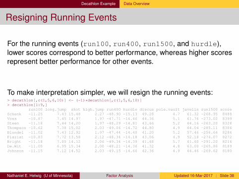
Resigning Running Events

For the running events (run100, run400, run1500, and hurdle),lower scores correspond to better performance, whereas higher scoresrepresent better performance for other events.

To make interpretation simpler, we will resign the running events:> decathlon[,c(1,5,6,10)] <- (-1)*decathlon[,c(1,5,6,10)]> decathlon[1:9,]

run100 long.jump shot high.jump run400 hurdle discus pole.vault javelin run1500 scoreSchenk -11.25 7.43 15.48 2.27 -48.90 -15.13 49.28 4.7 61.32 -268.95 8488Voss -10.87 7.45 14.97 1.97 -47.71 -14.46 44.36 5.1 61.76 -273.02 8399Steen -11.18 7.44 14.20 1.97 -48.29 -14.81 43.66 5.2 64.16 -263.20 8328Thompson -10.62 7.38 15.02 2.03 -49.06 -14.72 44.80 4.9 64.04 -285.11 8306Blondel -11.02 7.43 12.92 1.97 -47.44 -14.40 41.20 5.2 57.46 -256.64 8286Plaziat -10.83 7.72 13.58 2.12 -48.34 -14.18 43.06 4.9 52.18 -274.07 8272Bright -11.18 7.05 14.12 2.06 -49.34 -14.39 41.68 5.7 61.60 -291.20 8216De.Wit -11.05 6.95 15.34 2.00 -48.21 -14.36 41.32 4.8 63.00 -265.86 8189Johnson -11.15 7.12 14.52 2.03 -49.15 -14.66 42.36 4.9 66.46 -269.62 8180


Decathlon Example Estimate Factor Loadings

Factor Analysis Scree Plot

●

●

●

●●

●

1 2 3 4 5 6

0.1

0.2

0.3

0.4

FA Scree Plot

# Factors

Pro

port

ion

of V

aria

nce

famods <- vector("list", 6)for(k in 1:6) famods[[k]] <- factanal(x=decathlon[,1:10], factors=k)vafs <- sapply(famods, function(x) sum(x$loadings^2)) / nrow(famods[[1]]$loadings)vaf.scree <- vafs - c(0, vafs[1:5])plot(1:6, vaf.scree, type="b", xlab="# Factors",

ylab="Proportion of Variance", main="FA Scree Plot")


Decathlon Example Estimate Factor Loadings

FA Loadings: m = 2 Common Factors

−0.4 −0.2 0.0 0.2 0.4 0.6 0.8 1.0

−0.

40.

00.

20.

40.

60.

81.

0

Factor Loadings

F1 Loadings

F2

Load

ings

run100long.jump

shot

high.jump

run400

hurdle

discus

pole.vaultjavelin

run1500

score

2 4 6 8 10

0.1

0.2

0.3

0.4

0.5

0.6

0.7

Factor Uniquenesses

Variable (Xj)U

niqu

enes

s (ψ

j)

run100

long.jump

shot

high.jump

run400

hurdle

discus

pole.vault

javelin

run1500

score

> famod <- factanal(x=decathlon[,1:10], factors=2)> names(famod)[1] "converged" "loadings" "uniquenesses" "correlation"[5] "criteria" "factors" "dof" "method"[9] "rotmat" "STATISTIC" "PVAL" "n.obs"

[13] "call"


Decathlon Example Estimate Factor Scores

FA Scores: m = 2 Common Factors

●●

●● ●●● ●●●●● ●●●●

● ● ●●●●●● ●

● ●●

●●●

●●

●

−3 −2 −1 0 1

5500

6500

7500

8500

Weighted Least Squares Method

F1 Score

Dec

athl

on S

core

●●

●● ●●● ●●●●● ●●●●

● ● ●●●●●● ●

● ●●

●●●

●●

●

−2 −1 0 1

5500

6500

7500

8500

Regression Method

F1 ScoreD

ecat

hlon

Sco

re

> # refit model and get FA scores (NOT GOOD IDEA!!)> famodW <- factanal(x=decathlon[,1:10], factors=2, scores="Bartlett")> famodR <- factanal(x=decathlon[,1:10], factors=2, scores="regression")> round(cor(decathlon$score, famodR$scores), 4)

Factor1 Factor2[1,] 0.7336 0.6735> round(cor(decathlon$score, famodW$scores), 4)

Factor1 Factor2[1,] 0.7098 0.6474


Decathlon Example Oblique Rotation

FA with Oblique (Promax) Rotation

−0.4 −0.2 0.0 0.2 0.4 0.6 0.8 1.0

−0.

40.

00.

20.

40.

60.

81.

0

Varimax Factor Loadings

F1 Loadings

F2

Load

ings

run100long.jump

shot

high.jump

run400

hurdle

discus

pole.vaultjavelin

run1500

score

−0.4 −0.2 0.0 0.2 0.4 0.6 0.8 1.0

−0.

40.

00.

20.

40.

60.

81.

0

Promax Factor Loadings

F1 LoadingsF

2 Lo

adin

gs

run100long.jump

shot

high.jump

run400

hurdle

discus

pole.vault

javelin

run1500

score

> famod.promax <- promax(famod$loadings)> tcrossprod(solve(famod.promax$rotmat)) # correlation between rotated factor scores

[,1] [,2][1,] 1.0000000 0.4262771[2,] 0.4262771 1.0000000


Decathlon Example Oblique Rotation

FA with Oblique (Promax) Rotation, continued# compare loadings> oldFAloadings <- famod$loadings> newFAloadings <- famod$loadings %*% famod.promax$rotmat> sum((newFAloadings - famod.promax$loadings)^2)[1] 1.101632e-31

# compare reproduced data before and after rotation> oldFAscores <- famodR$scores> newFAscores <- oldFAscores %*% t(solve(famod.promax$rotmat))> Xold <- tcrossprod(oldFAscores, oldFAloadings)> Xnew <- tcrossprod(newFAscores, newFAloadings)> sum((Xold - Xnew)^2)[1] 3.370089e-30

# population and sample factor score covariance matrix (after rotation)> tcrossprod(solve(famod.promax$rotmat)) # population

[,1] [,2][1,] 1.0000000 0.4262771[2,] 0.4262771 1.0000000> cor(newFAscores) # sample

[,1] [,2][1,] 1.0000000 0.4563499[2,] 0.4563499 1.0000000Nathaniel E. Helwig (U of Minnesota) Factor Analysis Updated 16-Mar-2017 : Slide 43

Factor Analysis - users.stat.umn.eduusers.stat.umn.edu/~helwig/notes/factanal-Notes.pdf · 3 Theory...

Documents

Transcript of Factor Analysis - users.stat.umn.eduusers.stat.umn.edu/~helwig/notes/factanal-Notes.pdf · 3 Theory...