University of Central Florida University of Central Florida

STARS STARS

Retrospective Theses and Dissertations

1987

Experimental Verification of Laser Speckle Power Spectral Density Experimental Verification of Laser Speckle Power Spectral Density

Christopher T. Chiles University of Central Florida

Part of the Engineering Commons

Find similar works at: https://stars.library.ucf.edu/rtd

University of Central Florida Libraries http://library.ucf.edu

This Masters Thesis (Open Access) is brought to you for free and open access by STARS. It has been accepted for

inclusion in Retrospective Theses and Dissertations by an authorized administrator of STARS. For more information,

please contact STARS@ucf.edu.

STARS Citation STARS Citation Chiles, Christopher T., "Experimental Verification of Laser Speckle Power Spectral Density" (1987). Retrospective Theses and Dissertations. 5064. https://stars.library.ucf.edu/rtd/5064

EXPERIMENTAL VERIFICATION OF LASER SPECKLE POWER SPECTRAL DENSITY

BY

CHRISTOPHER TODD CHILES B.S.E.E., Ohio Northern University, 1982

RESEARCH REPORT

Submitted in partial fulfillment of the requirements for the degree of Master of Science in Engineering

in the G~aduate Studies Program of the College of Engineering University of Central Florida

Orlando, Florida

Spring Term 1987

ABSTRACT

The dependence of laser speckle power spectral density on the

autocorrelation of the aperture pupil function was verified using a

charge injection device (CID) camera. Speckle patterns acquired by

the CID array were processed to compute the power spectral density

(PSD). Three aperture shapes were studied. There was good agreement

between the theoretical and experimental power spectral density

shapes, and the cutoff frequencies agreed within five percent error.

ACKNOWLEDGEMENTS

In the many years I spent in obtaining this master's, I must

thank my wife Beth Ann and my son Micah in suffering through. the

long hours away from home. They cheerfully put up with the many

sacrifices. In addition, I must thank God for sustaining me and

giving me the perserverance.

My advisor, Dr. Glenn Boreman, has always been there with

advice, and the constant encouragement needed to complete the task,

and he deserves many thanks. Also, the electrical engineering

department at the University of Central Florida deserve much

gratitude for professionalism shown during my studies there.

Finally, LT Pat Heron deserves thanks for writing the driving

routines used in the speckle analysis program.

iii

LIST OF FIGURES

LIST OF TABLES

I. INTRODUCTION

TABLE OF CONTENTS

II. OPTICAL DESIGN OF THE INSTRUMENT

III. CHARGE INJECTION DEVICES AND CAMERA OPERATION

IV. DATA PROCESSING

V. EXPERIMENTAL RESULTS ..... .

VI. CONCLUSIONS AND RECOMMENDATIONS

APPENDIX A: TABULATED DATA

APPENDIX B: COMPUTER PROGRAM

iv

v

. . . vi

1

8

• . . 18

23

• • • • . • 27

• • • 36

• . • 38

42

LIST OF TABLES

1. National Television Systems Committee Standards . . . 20

2. Data Summary for Apertures . . . . . . . . 28

3. Experimental data for Figure . . . . . . . . . . 39

4. Experimental data for Figure . . . . . . 40

5. Experimental data for Figure . . . . . . . . . . . . 41

v

LIST OF FIGURES

1. Typical Laser Speckle Pattern

2. Typical Power Spectral Density Plot

3. Laser Speckle System Schematic .

4. System Block Diagram

5. Geometry for Diffraction Calculations

6. Aperture Shapes and Dimensions

7. Calculated Power Spectral Densities

8. Plot of Spatial Noise on CID array

9. Power Spectral Density Plot of Noise Waveform

10. Basic Geometry of CID pixel and Cross Section

11. Pixel Read Operation and Scanning

12. One Sample PSD . . . . . . 13. Twenty Sample PSD . . 14. Data for 1.0 cm Aperture at 1.0 m

15. Data for 1.6 cm Aperture at 1.5 m

16. Data for Double Slit Aperture at 1.0 m

vi

. .

. . . . . . .

• 2

• 3

• 5

• 6

10

15

16

17

17

19

21

25

25

30

32

34

I. INTRODUCTION

The statistics of laser speckle have been experimentally

verified (McKechnie 1974; Goldfischer 1965). Today the applications

of laser speckle include the determination of optical system

transfer functions (Boreman 1984), studying the mechanical

properties of materials (Khetan and Chiang 1976), and optical signal

processing (Francon 1984). In the cited studies, either a scanning

aperture or photographic film was used to record the speckle

pattern. The speckle pattern was then processed to compute the

autocorrelation of the speckle pattern, or the PSD of the pattern.

In both cases, the methods employed were cumbersome and consumed a

great deal of time. In this research report, a General Electric CID

camera acquired the laser speckle patterns and an Intel System 310

computer was used to calculate the PSD. An optical system was

designed and software written to experimentally verify the

dependence of the laser speckle PSD on the autocorrelation of the

aperture pupil function .

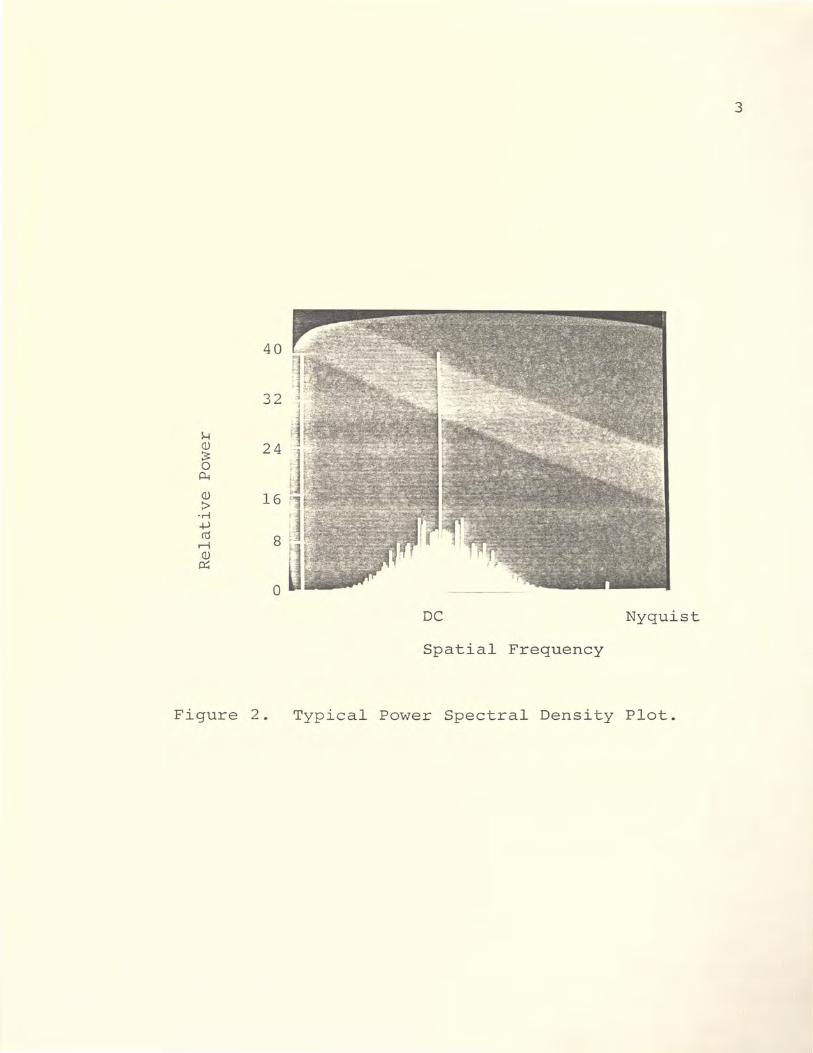
A typical speckle pattern is shown in Figure 1 on the following

page. In the experiment, a horizontal line of the pattern was

digitally recorded,

typical PSD plot

and then processed to calculate the

is shown in Figure 2. The vertical

PSD. A

axis is

relative power in abitrary units and the horizontal axis is spatial

frequency. The large spike in the center of the picture corresponds

2

Figure 1. Typical Laser Speckle Pattern.

3

32

~ <l) 24 3: 0

P-!

<l) 16 > ·r-1 +J cU

r-1 <l) ~

0

DC Nyquist

Spatial Frequency

Figure 2. Typical Power Spectral Density Plot.

4

to zero spatial frequency (DC), and the far right side of the

picture is the Nyquist freqency for the number of samples used.

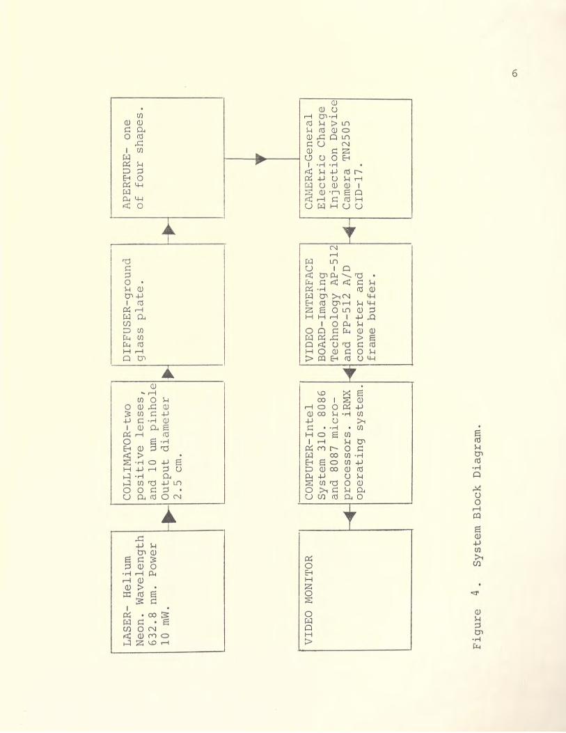
Figure 3 displays a system schematic, and Figure 4 is a block

diagram illustrating the major system components.

The speckle pattern of Figure 1 is the result of the random

interference of a dephased coherent wave front after passing through

a diffusing medium. In the system used, reference Figure 4, the

coherent waves (laser light) are generated using a 10 milliwatt

helium neon laser with a wavelength of 632.8 nanometers. The laser

beam is sent through a collimator which removes undesirable

intensity artifacts of the laser beam, and expands the beam's

diameter to 2.5 cm. The diffusing medium was a ground glass slide

whose surface roughness caused random phase retardations of the

wavefront. After transmission through the diffuser, the laser beam

impinged on an aperture designed to control the PSD of the speckle

pattern. Located in the Fresnel region of the aperture was a

General Electric TN 2505 CID-17 Camera. The camera converts the

irradiance pattern on the CID array to analog video signal

compatible with NTSC (National Television Systems Committee)

standards. In order to digitally process the speckle pattern, an

Imaging Technology video board, located inside the Intel computer,

converted a frame of camera information into a 512 x 512 x 8 bit

array. This information was processed by a Fortran 86 program

running under the iRMX operating system on the Intel computer. The

program allowed the irradiance pattern to be plotted, the PSD to be

DIF

FU

SE

R

CID

A

RR

AY

1-----

LA

SER

C

OL

LIM

AT

OR

A

PER

TU

RE

C

AM

ERA

C

OM

PUTE

R

Fig

ure

3

. L

ase

r S

peck

le

Sy

stem

S

ch

em

ati

c.

U1

LA

SE

R-

Heli

um

N

eon

. W

av

ele

ng

th

63

2.8

nm

. P

ow

er

10

mW

.

VID

EO

M

ON

ITO

R

CO

LL

IMA

TO

R-t

wo

po

sit

ive

len

ses,

an

d

10

um

pin

ho

le

~i O

utp

ut

dia

mete

r I~

2.5

cm

.

DIF

FU

SE

R-g

rou

nd

g

lass p

late

.

CO

MP

UT

ER

-In

tel

VID

EO

IN

TE

RFA

CE

S

yst

em

3

10

. 8

08

6

BO

AR

D-I

mag

ing

an

d

80

87

m

icro

-T

ech

no

log

y

AP

-51

2

~

~processors.

iRM

X

an

d

FP

-51

2

A/D

~

op

era

tin

g

syst

em

. co

nv

ert

er

an

d

fram

e

bu

ffer.

Fig

ure

4

Sy

stem

B

lock

D

iag

ram

.

APE

RT

UR

E-

on

e

of

fou

r sh

ap

es.

• C

AM

ER

A-G

ener

al

Ele

ctr

ic

Ch

arg

e

Inje

cti

on

D

ev

ice

Cam

era

TN

2505

C

ID-1

7.

m

calculated and plotted, and ensemble averaging of a series of

speckle patterns. The research report discusses the optical

design of the instrument in Section II, the operation of CID cameras

in Section III, the data processing in Section IV, and

experimental results in Section V. Conclusions and recommendations

are in Section VI. Appendix A contains the experimental data, and

the computer program is contained in Appendix B.

7

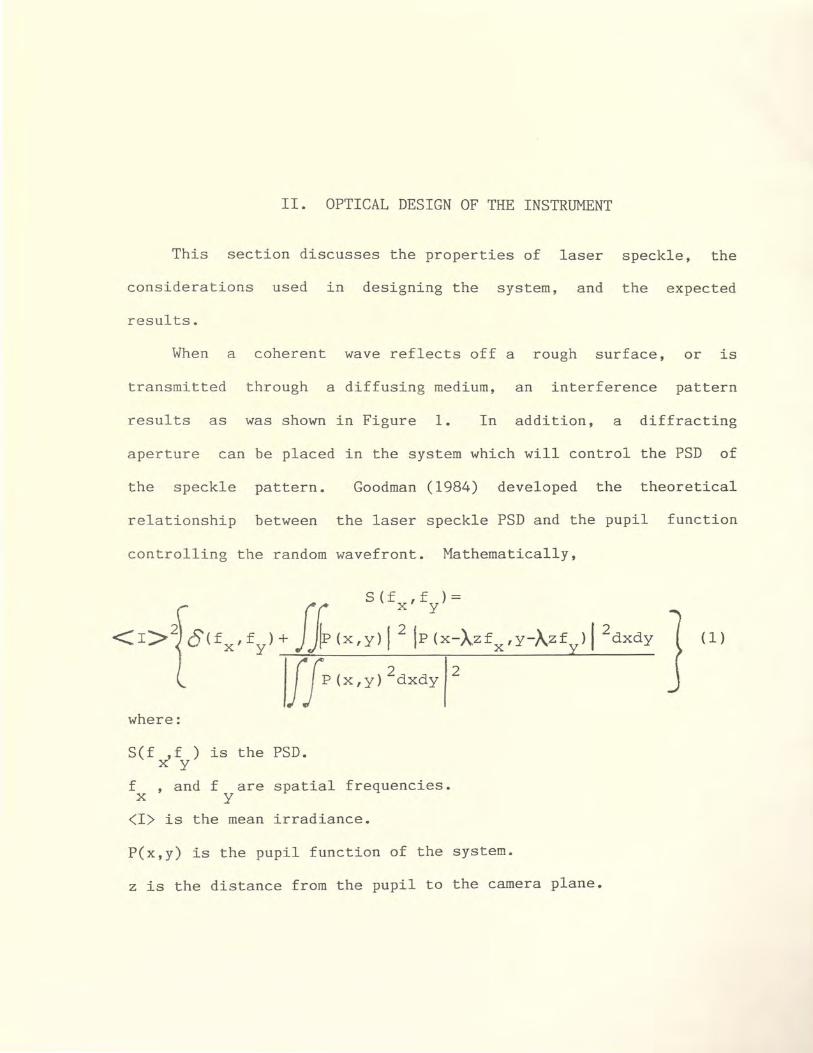
II. OPTICAL DESIGN OF THE INSTRUMENT

This section discusses the properties of laser speckle, the

considerations used in designing the system, and the expected

results.

When a coherent wave reflects off a rough surface, or is

transmitted through a diffusing medium, an interference pattern

results as was shown in Figure 1. In addition, a diffracting

aperture can be placed in the system which will control the PSD of

the speckle pattern. Goodman (1984) developed the theoretical

relationship between the laser speckle PSD and the pupil function

controlling the random wavefront. Mathematically,

S(f ,f )=

<::I:::>-2 Q<fx,fy)+ ~~(x,y)I ~ IP:x-Azfx,y-Azfy)I

2dxdy

~~P(x,y) 2dxdy 2

where:

S(f ,f ) is the PSD. x y

f , and f are spatial frequencies. x y

<I> is the mean irradiance.

P(x,y) is the pupil function of the system.

z is the distance from the pupil to the camera plane.

( 1 )

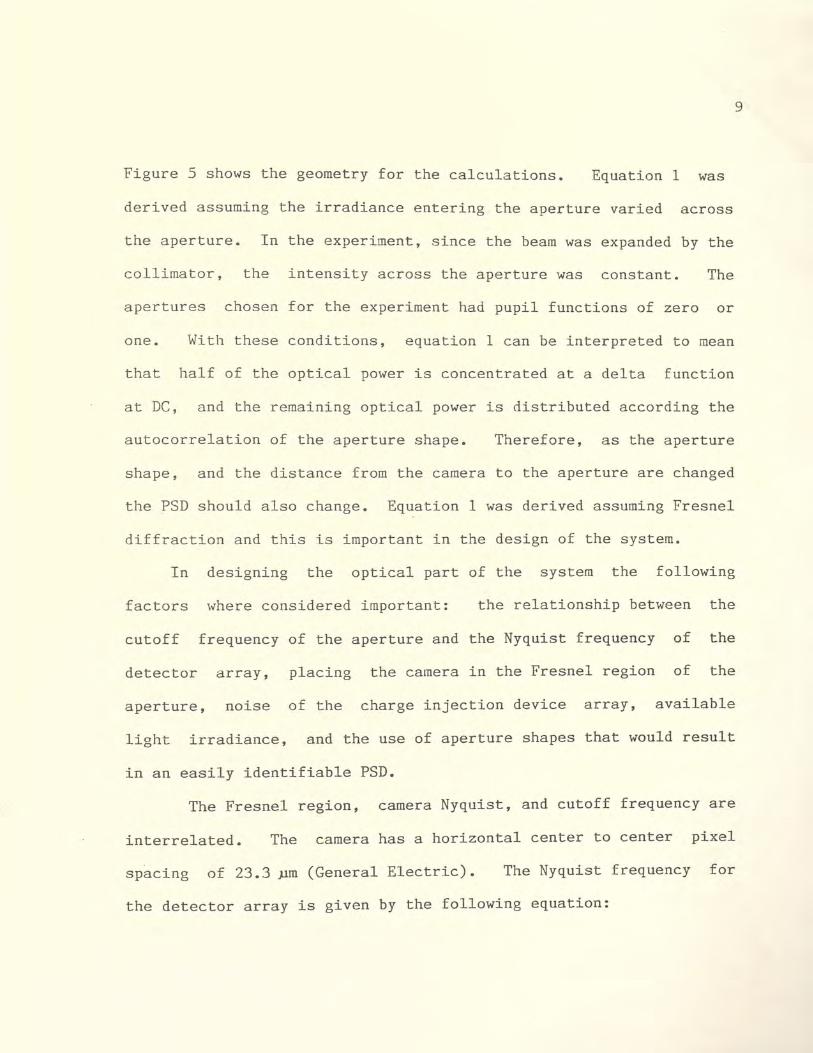
Figure 5 shows the geometry for the calculations. Equation 1 was

derived assuming the irradiance entering the aperture varied across

the aperture. In the experiment, since the beam was expanded by the

collimator, the intensity across the aperture was constant. The

apertures chosen for the experiment had pupil functions of zero or

one. With these conditions, equation 1 can be interpreted to mean

that half of the optical power is concentrated at a delta function

at DC, and the remaining optical power is distributed according the

autocorrelation of the aperture shape. Therefore, as the aperture

shape, and the distance from the camera to the aperture are changed

the PSD should also change. Equation 1 was derived assuming Fresnel

diffraction and this is important in the design of the system.

In designing the optical part of the system the following

factors where considered important: the relationship between the

cutoff frequency of the aperture and the Nyquist frequency of the

detector array, placing the camera in the Fresnel region of the

aperture, noise of the charge injection device array, available

light irradiance, and the use of aperture shapes that would result

in an easily identifiable PSD.

The Fresnel region, camera Nyquist, and cutoff frequency are

interrelated. The camera has a horizontal center to center pixel

spacing of 23.3 pm (General Electric). The Nyquist frequency for

the detector array is given by the following equation:

9

DIF

FU

SE

L

ASE

R

LIG

HT

f ·

-an

=

.. ~~~. ~

----,~~~~-··-

--

·---

·-~~---~--

--------

z

y

x

r /

P(

x,y

)

v

/'

/ /u

APE

RT

UR

E

PLA

NE

C

AM

ERA

PL

AN

E

Fig

ure

5

. G

eom

etry

fo

r d

iffr

acti

on

calc

ula

tio

ns.

1-1

0

11

( 2)

where:

fN is the Nyquist frequency.

f::::.x is the center to center pixel spacing.

This gives a Nyquist frequency of 21.5 cycles/mm. Therefore, the

aperture width, and distance to the camera, should give a speckle

pattern with a cutoff frequen~y below this value, and also some

allowance was made to keep the spatial bandwith narrow enough that

the modulation transfer function of the camera could be assumed to

unity. Also, consideration was given to the available length on

the optical table, and diameter of the collimator. The collimator

had a diameter of 2.5 cm, and to be able to assume the aperture was

uniformly illuminated, the maximum aperture width was limited to 1.6

cm. Once the maximum aperture width was chosen, diffraction theory

was used to calculate approximately the distance within which the

Fresnel approximation would be valid.

Following Goodman (1968), the field strength in the camera

plane is given by:

U(u,v)

where:

= 1 !JP (x,y)

j A-; aperture exp(jkr)dxdy ( 3)

U(u,v) is the field strength at the camera plane.

P(x,y) describes the aperture shape.

A is the wavelength of the light.

12

r is the distance from a point of the pupil plane to a point on the

camera plane.

The expression for r in terms of the geometry

r z~l + 2

(u-x) + z ( 4)

Using a binomial expansion for r, the expression can be approximated

by :

ux+vy x 2 +y 2

z + 2z

The Fresnel approximation uses all the above terms

( 5)

and the

Fraunhofer approximation retains the first three terms. The

distinction between the two approximations occurs when the phase

contribution of the quadratic term was greater than TT/2 (Fresnel),

or less than 7T /2 ( Fraunhofer). Therefore, to be within the

Fresnel region the maximum distance can be calculated by the

following equation (Lizuka 1985):

where:

L is the aperture width.

2 z>> L

A

13

(6)

For a 1.6 cm aperture the distance must be less than 4 m and for a

1 cm aperture the distance must be less than 1.58 m The other

consideration is where the Fresnel region starts. Goodman (1968)

approximates this by the condition that the next higher order term

in the binomial expansion must give a phase contribution of less

than one radian. Using this concept, the minimum distance can be

found by the following equation:

z 3 >::> 1T (u-x) 2 + (v-y) 2

] 2

(7) 4 maximum

For a 1.6 cm aperture, the minimum distance is approximately 27 cm,

and for a 1 cm aperture the minimum distance is 15 cm. Now, the

cutoff frequency for the laser speckle PSD is given (Goodman 1984):

f = co L ( 8)

14

The aperture widths were chosen to be 1.6 and 1 cm for illumination

considerations, so the cutoff frequencies were determined by the

distance z. To allow some error in the aperture widths, and the

measured distance, the cutoff frequency was designed to be,

approximately, .75 of the array Nyquist, or 16 cycles/mm.

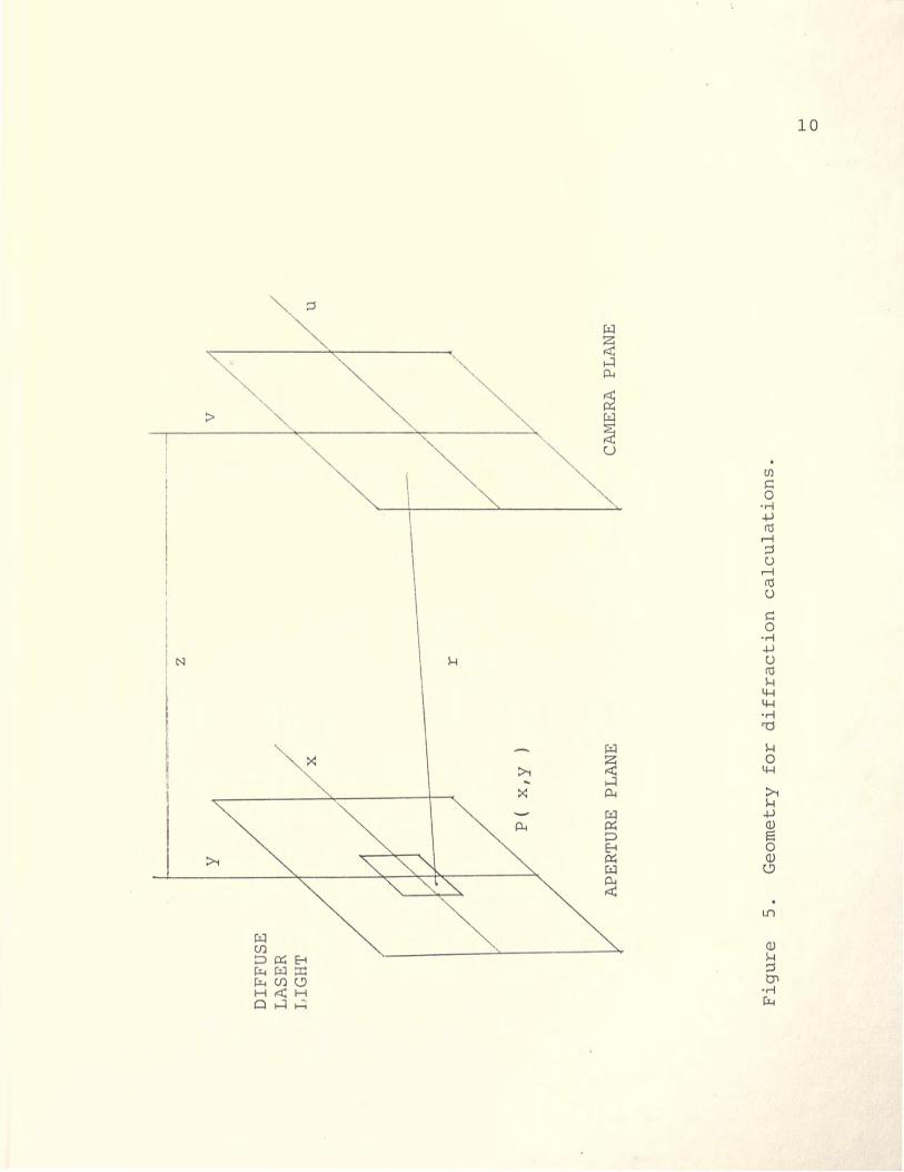
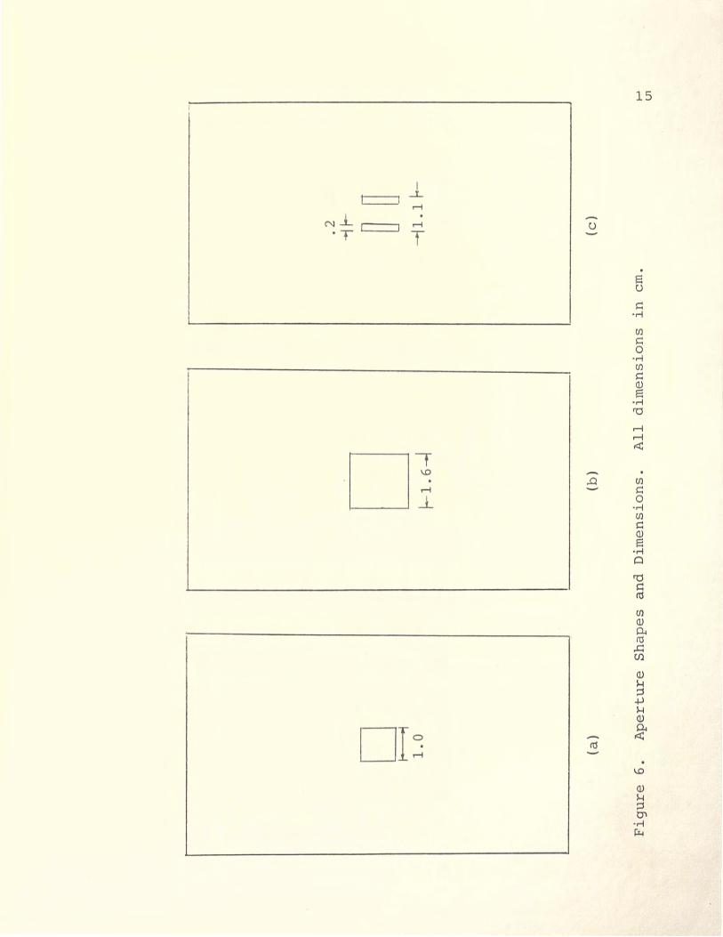
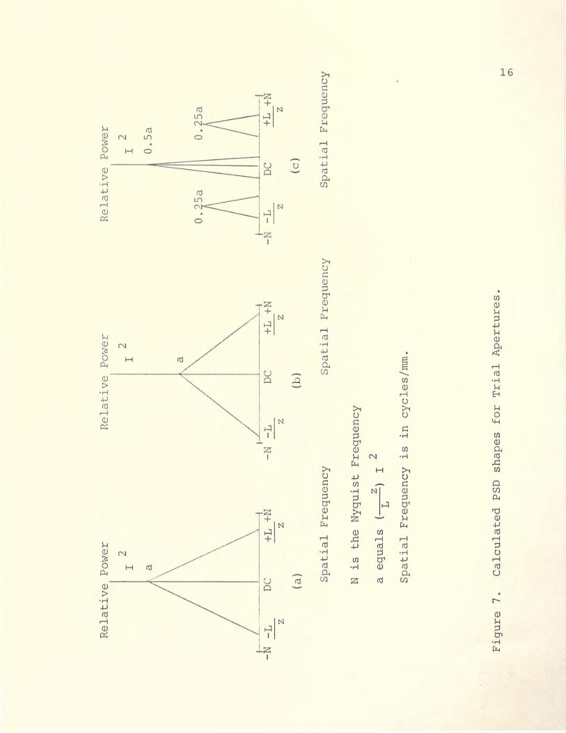
The aperture shapes were chosen based upon there expected PSD.

For a square aperture, the expected PSD shape is triangular, which

is easily recognizable. A double slit was also tried. Figures 6

and 7 show the shapes, dimensions, and expected results. The PSD

calculations followed Goodman (1984).

With the aperture widths and camera distance now fixed, sample

speckle patterns were generated in the laboratory to check for well

developed speckle patterns (a speckle pattern is well developed if

the pattern has well defined dark spots). The available light

intensity on the aperture, and CID noise were not significant

problems. The irradiance on the CID array was great enough to keep

the mean signal level much larger than the dark current noise of the

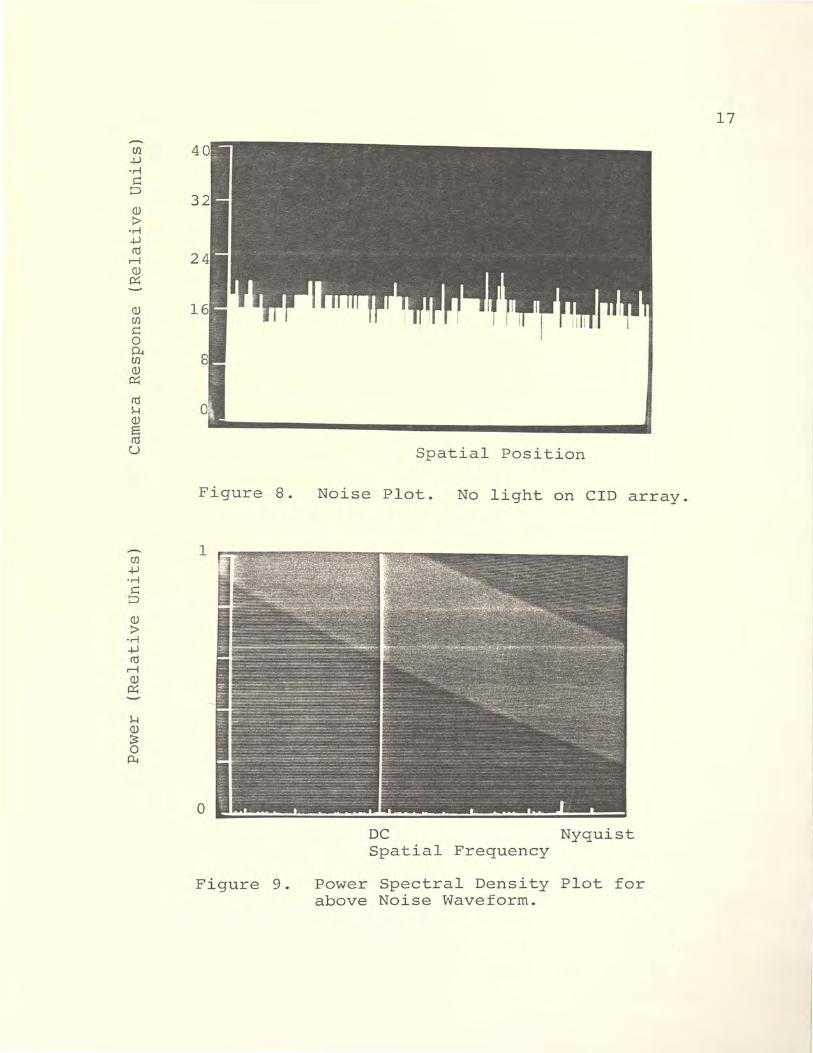
array. Figure 8 shows a typical pixel scan of the detector noise

with the charge injection array in darkness. The mean noise level

is approximately 16 units (on a scale from 0-255), with a variance

of 1. The photograph below, Figure 9, is a PSD plot. Due to the

uniform nature of the noise, most of the noise power is concentrated

in the DC component, and had almost no effect on the power spectral

density plots for the apertures. Based upon this data, noise was

not considered a problem.

D ~

D

1.

0 ~1.6~

(a)

(b)

Fig

ure

6

. A

pert

ure

S

hap

es

and

D

imen

sio

ns.

A

ll

dim

en

sio

ns

in

cm.

• 2

~I- ~ ~

-jl.

l ~

( c)

~

V1

Rela

tiv

e

Po

wer

R

ela

tiv

e

Pow

er

I 2

I 2

-fJ-=

i _

__

___..._

_,

DC

+L

+N

-N

-L

<

~-

t

+L

+N

DC

z z

z z

(a)

(b)

Sp

ati

al

Fre

qu

ency

S

pati

al

Fre

qu

ency

N i

s

the

Ny

qu

ist

Fre

qu

ency

z 2

a eq

uals

(~L~)

I

Sp

ati

al

Fre

qu

ency

is

in

cy

cles

/mm

.

Fig

ure

7

. C

alc

ula

ted

PS

D

shap

es

for

Tri

al

Ap

ert

ure

s.

Rela

tiv

e

Po

wer

I 2

O.S

a

0.2

5a

I I

_J _

_ j_

__

i_ __

L_~-1

-N

-L

DC

+L

+N

z z

( c)

Sp

ati

al

Fre

qu

ency

~

m

en _µ .,..; ~

:::::>

<J)

:> .,..; _µ co

r-1 <J)

p::;

1"-l <J)

~ 0 0-!

Figure 8.

1

0

Figure 9.

Spatial Position

Noise Plot. No light on CID array.

DC Nyquist Spatial Frequency

Power Spectral Density Plot for above Noise Waveform.

17

6

III. CHARGE INJECTION DEVICES AND CAMERA OPERATION

In the 1970s, charge coupled and charge injection devices were

developed (Hall 1980). They operate on charge collection under the

surface of a metal oxide semiconductor (MOS) capacitor which is

appropriately biased. The charge collected can either be

electrically injected, or could be generated optically. Hence, in

the rapid development that followed their introduction, the use of

charge coupled devices (CCDs) and charge injection devices (CIDs) as

solid state imaging devices has become common. General Electric has

pioneered the use of CIDs for imaging, and as a result of their

research, they developed the TN2505 camera used in this experiment.

The following description and discussion of operation is a

summarization of several published articles, and the camera

technical manual (Lunden et al. 1983 and Carbone et al. 1983)

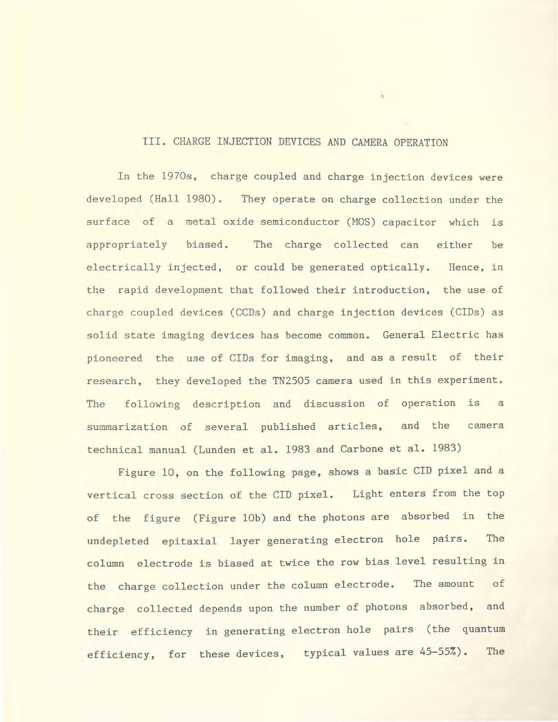
Figure 10, on the following page, shows a basic CID pixel and a

vertical cross section of the CID pixel. Light enters from the top

of the figure (Figure lOb) and the photons are absorbed in the

undepleted epitaxial layer generating electron hole pairs. The

column electrode is biased at twice the row bias level resulting in

the charge collection under the column electrode. The amount of

charge collected depends upon the number of photons absorbed, and

their efficiency

efficiency, for

in generating electron hole pairs (the quantum

these devices, typical values are 45-55%). The

Figure lOa.

I I

IMAGINARY PIXEL BOUNDARY

ALUMINUM STRAP

Geometry of CID Pixel.

COLUMN ROW FIE LD ITHICKPOL YI tTH INPOLYI OX IDE

_JI L ----- ~ _J 5µ '----'

Figure lOb.

N-EPITAXIAL LA YER

P-SUBSTRATE

Vertical Cross Section of CID Cell.

19

Above diagrams courtesy of General Electric Co.

20

charge collected is periodically sensed so that the voltage

generated is a function of the number of photons per time, or the

irradiance of the light. When a line of pixels is scanned, the

column electrode is biased to its minimum level causing the stored

charge to flow to the row electrode (see Figure 11 a). This causes

a displacement current, proportional to the collected charge, which

is sensed by a differential current amplifier. Once all the pixels

in a row have been read, the row electrodes are biased to a minimum

voltage injecting the charge into the substrate, and clearing the

pixel line for the next sampling interval. Note, the charge sensing

process is nondestructive, and future applications could make use of

this feature. The present row being scanned, and the previous row

are connected to the differential amplifier. This eliminates

voltage offset due to row selection noise, and fixed pattern noise

generated by structural, or electrical irregularities. Figure llb

illustrates the pixel arrangment and scanning methods. The camera

used was designed to be compatible with standards developed by the

National Television Systems Committee (NTSC). Table 1 contains the

salient points of the standard (Shanrnugam 1979).

TABLE 1 National Television Systems Committee Standards

Aspect ratio Total lines/frame line rate line time Horizontal retrace Vertical retrace Picture information/frame

4/3 525/frame 15,750 lines/sec 63.5 usec 10 usec 1.27 msec 485 lines/frame

COL

ROW

,------, I ,--,... ;- _. /,/ .. -,.. ~\

: ~I' , , , / ) READOU T

~ O S

•:> s INJECTION

Figure lla. Read Operation of CID Cell.

PIXEL SCAN DIFFERENTIAL CURRENT SENSE AMPLIFIER

~

"' ;i 0 ...I

z 0 I-u w ...I w (/)

~ 0 a:

INJECTION CONTROL SIGNALS

Figure llb.

0

COLUMN

.---+~~.+==---.~~ ...... --__,. REFERENCE POTENTIAL

PARALLEL ROW &

'------..... -<. ACCESS

SIGNALS

Pixel Scanning Arrangement.

Above figures courtesy of General Electric Co.

21

22

The camera consists of three printed circuit boards containing very

large scale and large scale integrated circuits (VLSI and LSI) which

add the appropriate synchronization signals to the CID array

information. Referring to Table 1, there are only 485 lines/frame

which correspond to information. The CID array has 244 lines of

pixels. Thus, each line of pixels generates two video lines. To

achieve the necessary horizontal resolution, there are 377 pixels.

Consideration was given to the modulation transfer function (MTF) of

the camera. The manufacturer specifies a MTF of greater than 80% at

250 lines. The Nyquist frequency of the camera would be 377 lines.

By designing the cutoff frequency for the aperture to be at .75

Nyquist, the effect of the camera MTF was ignored. In other words,

the CID array was treated as a piece of photographic film recording

the speckle pattern.

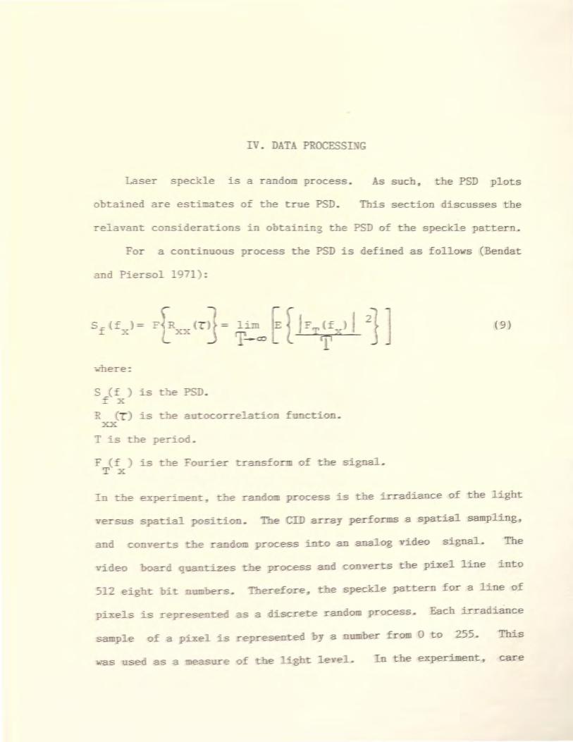
Laser speckle :s a ran

obtaine are es :ima es --r- :t e t_ e P

relava n .._ cons_::_ era~ · o s

'-'or a c t. 4

uo

and p_::_ers 1 9 ) ..

r s_ ( :f } = FR

I :_ XX

wh ere :

,c ( )

:xx

is e Jleri

a~g

P- .c:ess

f c: i

ess. As s c~ , the PSD plots

s section discusses the

of the speckle pattern.

is efine as follows (Bendat

2 (9)

<= ) :is - x

o:f t J. e s_::gna:I

- .., e ran ess :i:s the irradiance of the light

·e sus s t:ial siti e i ar.:=-a _performs a spatial sampling,

and ~o erts era m r ess :_t an ~na og i eo sig al. he

·vi eo boar iz'es t ·e r cess a con1"erts the pixel line into

512 eig it um e s . _here£ _ve e s _ ec -e ;>:at e f o a line of

ixels i s re_l)re-sente1.:: ::as a iscrete ran _Each irradiance

sam le £a is repre-se ed mbe £ro 0 to 255. This

was se as a meas e £ the _igh e :exper ent care

24

was taken so that the CID array was not saturated. So the data

obtained was a a true reflection of the light level. To calculate

the PSD of a discrete process, the following equation was used

(Bendat and Piersol 1971):

(10)

FN (fx ) is the discrete Fourier transform (DFT) of the irradiance

samples, and N is the number of samples. In the experiment N=512,

so spatial frequencies are calculated from -255 to +255. Frequency

component 255 is the Nyquist frequency. In the computer program,

the division by N was not performed since it is essentially a

scaling factor.

Since the process observed was random in nature, one record or

line sample is not sufficient in calculating the PSD. In order to

obtain a good estimate, it is necessary to average over many speckle

patterns. The effect of this ensemble averaging is demonstrated on

the following page by Figures 12 and 13. Figure 12 is a PSD plot

for one record of a square aperture. Figure 13 is a twenty record

average of the same aperture. Notice how the PSD has smoothed out

and has a triangular shape. In general, as the number of records

averaged increases the PSD estimate becomes better. In the

experiment, an average of twenty records was used for each aperture

shape based upon experience and experimental evidence.

25

DC Nyquist Spatial Frequency

Figur~ 12. One Sample PSD.

DC Nyquist Spatial Frequency

Figure 13. Twenty Sample Average PSD.

26

The method used was a modification of the method outlined by

Bendat and Piersol in Random Data: Analysis and Measurement

Procedures (1971). The method is as follows:

1. Taper the data using a window function.

2. Compute the DFr (the program used an FFT routine).

3. Calculate the PSD.

In practice, it was found the windowing did not significantly

improve the PSD estimate. Windowing did not have a large effect

because the PSD's observed did not have a large high frequency

content, and this is where the effect of windowing would be

observed. Once a PSD for a sample was calculated, the diffuser was

moved, and a new sample taken. This process was repeated until the

desired number of samples was obtained. Once all the individual

PSDs were calculated, they were then averaged to obtain the final

estimate of the PSD.

V. EXPERIMENTAL RESULTS

There was good agreement between the calculated and

experimental characteristics of the laser speckle power spectral

density. The three data trials gave expected cutoff f r equencies

within 5 percent in all cases. Figures 14-16, on the following

pages display the experimental results.

Table 2 summarizes the calculated and experimental cutoff

frequencies. Note the experimental column has the term corrected.

During the processing of the data, consideration was given to the

effect of translating 377 data points from the video line into 512

digital numbers. The effect caused the relationship between the

actual spatial frequencies, and the displayed spatial frequencies to

be scaled by a factor of 512/377. It also results in the displayed

Nyquist frequency (right edge , of the power spectral density

photographs) not to be the true Nyquist frequency of the array. To

correct for this effect, the displayed frequency was scaled by

512/377. To calculate the experimental cutoff frequencies, the

ratio of the displayed cutoff frequency to the displayed Nyquist

frequency was calculated. This was done by physically measuring the

distances on the photograph, and also checking against scanned

frequency components during the data trials. This ratio was

multiplied by the actual Nyquist frequency of the CID array, and

then scaled by 512/377 to obtain the final cutoff frequency in

28

TABLE 2

DATA SUMMARY FOR APERTURES

SHAPE WIDTH(L) DISTANCE(Z) CUTOFF FREQ. CUTOFF FREQ. (CM) (CM) CALCULATED EXPERIMENTAL

(CYCLES/MM) (CORRECTED) (CYCLES/MM)

SQUARE 1 100 15.8 15.7 1.6 150 16.9 15.5

DOUBLE 1.0 100 15.8 15.5

29

cycles/mm • A second effect was also observed. Notice on the power

spectral density plots (Figures 14d,15d,16d) there is a small spike

at approximately .75 Nyquist. The actual frequency component is

number 188, or 255(377/512). Frequency component 255 is the highest

calculated frequency for the 512 point FFT used in the computer _______ ___.;

program, and is the displayed Nyquist frequency. The small spike ··-shows the physical Nyquist frequency of the CID array. Figure 14 is

the 1 cm. square aperture at lm. Figure 14b shows well developed

speckle pattern, figure 14c shows the data from line 235 of the

frame buffer, and figure 14d is the PSD plot. The general shape of

the PSD plot is triangular with a spike at de as was calculated.

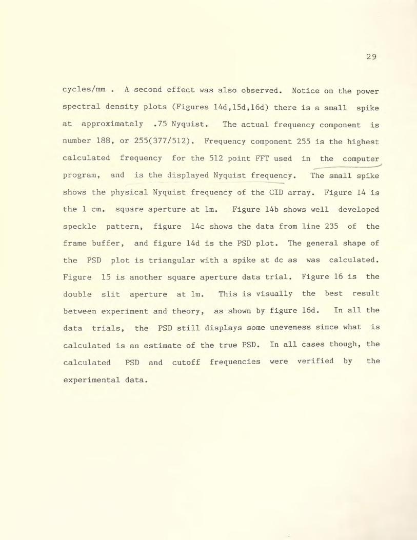
Figure 15 is another square aperture data trial. Figure 16 is the

double slit aperture at lm. This is visually the best result

between experiment and theory, as shown by figure 16d. In all the

data trials, the PSD still displays some uneveness since what is

calculated is an estimate of the true PSD. In all cases though, the

calculated PSD and cutoff frequencies were verified by the

experimental data.

Figure 14.

D

(a)

(b)

Square Aperture Data (lcm at lm) (a) Aperture Shape (b) Speckle Pattern (c) Irradiance Data (d) PSD

30

31

200 Q) 0 i:: 150 m

·r-1 ro m ~ lo-! 100 H

50

0

Spatial Position

( c)

30

24 ~ Q)

~ 0 0-l 18 Q)

:> ·r-1 .µ

12 m r-1 Q) p::;

6

DC Nyquist

Spatial Frequency

(d)

Figure 14. continued.

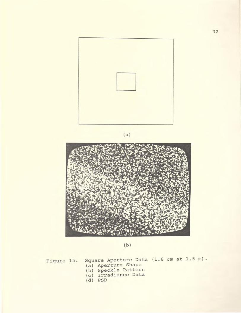
Figure 15.

D

(a·)

(b)

Square Aperture Data (1.6 cm at 1.5 rn). (a) Aperture Shape (b) Speckle Pattern (c) Irradiance Data (d) PSD

32

33

200

160

<1) 120

()

s:: '° ·r-1 80

"d

'° H H 40 H

0

Spatial Position

(c)

30

24

H <1)

:== 0 ~

<1) :>- 12 ·r-1 .µ

'° r-1 6 <1) o::;

0

DC Nyquist

Spatial Frequency

(d)

Figure 15. continued.

( a )

(b)

Figure 16 . Double Slit Aperture Data (lrn) (a) Aperture Shape (b) Speckle Pattern (c) Irradiance Data (d) PSD

34

r

100

Q) 80 0 ~ <U

· r-l ro 60 <U ~ ~

H 40

20

0

5

4

3

2

1

0

Figure 16 .

Spatial Position ( c)

DC

Spatial Frequency

(d)

continued .

35

Nyquist

VI. CONCLUSIONS AND RECOMMENDATIONS

The agreement between the theory and experiment was excellent.

The cutoff frequency values were within five percent, and the proper

shapes for the power spectral densities were observed. The only

consideration not anticipated was the effect of converting the CID

data (377 data points) into 512 data points. This could be resolved

by writing an algorithm to sort the digital information and

reconstruct the individual pixel information. Then a 512 point FFT

could be performed. In summary, the theory was verified.

Considering the great simplification in image detection and

processing brought about by the introduction of the CID cameras, the

possible applications are numerous. The CID array is essentially a

large analog storage register, which can be randomly accessed. A

little thought, along the line of image detection, leads one to many

ideas. For example, if a lens was put in front of the CID array to

perform a Fourier transform on an image, the individual pixels could

be read giving a sampling of the frequency spectrum. With the

liquid crystal technology that now exists, an adaptive spatial

filter could be constructed in the Fourier plane, being controlled

by the frequency sampling of the CID array through a computer.

Speckle has already found many uses, but the ability to shape

the power spectral density has great implications. Speckle can be

filtered in the Fourier plane, and could be used in a similar manner

37

as narrowband white noise is used in system transfer function

determination. One recommendation is to try filtering the power

spectral density of the laser speckle in the frequency domain,

instead of aperture shaping. Aperture shaping of the power spectral

density is limited due to the large de spike, and the natural

effects · of pupil function autocorrelation .

APPENDIX A

TABULATED DATA

38

39

TABLE 3

TRIAL DATA FOR 1 CM SQUARE APERTURE AT lM.

TRIAL MEAN INTENSITY VARIANCE (0-255)

1 73 1613 2 71 1493 3 65 1319 4 68 1419 5 66 1328 6 66 1422 7 70 1449 8 73 1892 9 75 2024

10 75 1998 11 71 1885 12 71 2136 13 73 1929 14 75 2082 15 74 1965 16 74 1800 17 68 1700 18 69 1395 19 69 1667 20 72 1560

40

TABLE 4

TRIAL DATA FOR 1.6 CM SQUARE APERTURE AT 1.5 M.

TRIAL MEAN INTENSITY VARIANCE (0-255)

1 63 925 2 59 767 3 56 674 4 58 940 5 54 632 6 57 803 7 60 1253 8 52 567 9 53 564

10 58 805 11 57 891 12 56 955 13 64 992 14 57 709 15 59 776 16 53 589 17 63 1047 18 59 750 19 53 597 20 62 1211

TABLE 5

TRIAL DATA FOR 1.1 CM DOUBLE SLIT APERTURE AT lM.

TRIAL

1 2 3 4 5 6 7 8 9

10 11 12 13 14 15 16 17 18 19 20

MEAN INTENSITY (0-255)

35 35 31 30 33 35 32 32 30 29 30 32 33 30 33 30 30 32 35 33

VARIANCE

183 144

66 52

201 150 262

99 56

105 49 68

102 74

144 87 94 75

125 112

41

APPENDIX B

SPECKLE ANALYSIS

PROGRAM

42

$STORAGE(INTEGER*2,LOGICAL*l) $PAGELENGTH(50)

PROGRAM SPECKLE c Laser Speckle image analysis program . c Copyright 1987 LT Christopher T. Chiles c and LT Patrick Heron U. S . Navy. c Driving subroutines developed by P. Heron and c main data analysis section developed by c C. Chiles. c Program is menu driven off the first letter of c the heading or as indicated on the menu. c Developed in Fortran86 for an Intel iRMX c Operating System . c c c c

c

Main Program Variable Definition

character*l fen

c Menu c

40 write(6,*)' write(6,*)' write(6,*)'Load memory /Redraw image/ Time average(y) write(6,*)' write(6,*)'Hove cursor /Plot intens ity(p) /Histogram' write(6,*)' write(6,*)' Grabframe / Aquire image' write(6,*)'

write(6,*)'Scan the results(s) /Multiple Runs(z)' write(6,*)' '

read(5,5)fcn 5 format(al)

if ((fcn.EQ. 'a' ) . OR . (fcn.EQ. 'A')) call output(#9009h,#11000000b) if ( (fcn.EQ. 'm') . OR. (fcn . EQ. 'M') ) call move if ( (fcn.EQ. 'p') .OR. (fcn.EQ. 'P') )call plot if ( (fcn.EQ . 'h') . OR. (fcn . EQ. 'H') )call h i st if ((fcn.EQ. 'r' ).OR. (fcn.EQ. 'R' ))ca ll re d raw if ((fcn . EQ. 'g' ).OR. (fcn.EQ. 'G' ))call grab if ((fcn.EQ. 'l' ) . or. (fcn.EQ. 'L' )) c all load

if ((fcn . EQ. 'y') .OR . (fcn . EQ. 'Y' ))call tavg if ((fcn.EQ.'s').OR.(fcn.EQ.'S'))call scan if ( (fcn.EQ. 'z') . OR. (fcn.EQ. 'Z') )call mrun go to 40

end

SUBROUTINE MRUN c Allows multiple runs of data and subtraction of power c spectra. Need to input the number of runs. c c c

Variable Declaration

integer*l n,nl,n2,frame(0:511,0:469),i complex*8 temp(O:l,0 : 511),x(512) integer*2 hole,xpos common frame,x,hole

write(6,*)' Input the number of runs,<4, (13)' read(5,10)n

10 format(I3) do 20 i=l.n

43

c c

c

c c c

c

writelci.~J ' execuLin~ run . ~ call tavg do 30 xpos=l,512

temp(i,xpos;=x(xpos) 30 continue 20 continue

write(6,*)'Runs are complete' write(6,*)'Which runs to subtract?' write(6,*)'Input base run(I3)' read(5,100)nl

lOQ format(I3) write(6,* ) 'Run to be subtracted?(I3)' read(5, 105)n2

105 format(I3) do 40 xpos = l,512

x(xpos)=temp(nl,xpos)-temp(n2,xpos) 40 continue

.; GO

500

100

110

115

505

520

call sketch return end

SUBROUTINE TAVG this subroutine calculates the average power spectral de nsity for a number of samples controlled by the ope rator.

variable declaration

integer*l frame(0:511,0:469),n,i integer*2 xpos,ypos,numb,sampn,hole real*'8 w,temp,d complex*8 x (5 12),spd(512),sum,tot,mean,variance character*l flag,flagl,flag2,flag3

common frame,x,hole

write(6.*)'what line number to scan(I3)?' read(5,400)hole format(I3) write(6,*)'number of samples to be taken(I3)' read(5,500)nwnb format(I3) write(6,*)'subtract mean?(y)' read(5,100)flagl format(al) write(6,*)'window?(y)' read(5,110)flag2 format(al) write(6,*)'smooth the psd?(y)' read(5,115)flag3 format( al) do 505 xpos=l,512 spd(xpos) = (0.0) continue do 510 sampn=l,numb

write(6,*)'sample number' ,sampn, '(type y and return )' read(5,520)flag format( al) if((flag.EQ. 'y' ).OR. (f l ag.EQ . 'Y' )) then

acquire the image

call output(~9009H,#11000000b)

44

c c

c c c

530 525

call grab

input and convert raw data

ypos=hole do 525 ypos=(hole-2 0 ), (hole+20) call outw(~9002H,ypos) do 530 xpos=0 , 511 call outw(~9000H,xpos) call input(~900EH,frarne(xpos,ypos)) continue continue call fetch

c calculate the rnean,subtract , and window

40 5

415

410

c

mean=(0 . 0,0 . 0) tot=(0.0,0 . 0)

do 405 xpos=l,512 tot =tot+x(xpos)

continue mean=tot / 512 . 0 variance=(0.0,0.0) do 415 xpos=l,512 variance=variance+(mean- x(xpos))**2 variance=variance/511.0 if ( ( f lagl. EQ. 'y ' ) . OR ( f lagl . EQ. 'Y' ) ) then do 410 xpos=l,512 x(xpos)=x(xpos) - mean continue end if write(6, * )'the mean was' ,real(mean) write(6,*)'the variance was' ,real(variance) call sketch if((flag2.EQ. 'y' ).OR. (flag2 . EQ. 'Y' ))then write(6,*)'windowing'

c t his is an extended cosine bell window.

420

425 c

c

550

510

560 c

do 420 xpos=l,51 w=cos(6.283185*(5*(xpo s -1)/511.0)) x(xpos) =x(xpo s )*(. 5*( 1 - w)) continue do 425 xpos=462,512 w=co s (6.283185*(5*(xpos-1)/511.0)) x(xpos)=x(xpos)*( . 5*(1-w)) continu e call s ketch

end if call fft call s ketch

do 550 xpos = l,512 x(xpos) = (x(xpos))**2 spd(xpos)=spd(xpos )+x(xpos)

continue end if continue

do 560 xpos=l,512 x(xpos)=spd(xpos)/nurnb

continue

c smooth the data c

565

if( (flag3.EQ. 'y') . OR . (flag3.EQ. 'Y') )then write(6, * )'number of frequencies to smooth(I3)?' read(5 , 565)n format(I3) write(6,*)'smoothing'

45

575

580 570

do 5 7 0 x po s = l , ( 5 1 2 - n ) sum= (0 .0,0.0) do 575 i=O,n

sum=sum+x(xpos+n) continue d=float(n+l)

do 580 i=O,n x(xpos+n)=sum/d

continue continue

end if call sketch return end

SUBROUTINE SCAN c This allows the operator to see the actual values c of the raw data of the output of tavg. c c

:o

Variable Declaration

real*4 s,threshold integer*2 xpos,ypos,hole integer*l frarne(0:511,0:469) complex-'8 x(512) common frame,x,hole

write(6,*)'Input scan threshold(real format)' read(5,*)threshold ~rite(6,*)'threshold=' ,threshold do 10 xpos=l,512

s=real(x(xpos)) ypos=xpos if ( s.GE.threshold)then

if(xpos.GT.256)ypos=512-xpos write(6,*)ypos,s · endif

continue return end

SUBROUTINE GRAB c Outputs signal to frame buffer to freeze c image.

call output(#9009h,#10000000b) end

SUBROUTINE HOVE c Moves the cursor so a line of data may c be scanned.

10 30

integer*l frame(0:511,0:469) integer*2 xpos,ypos,hole

complex*8 x(512) common frame,x,hole

write(6,*)' cursor position? write(6,*)' (format(I3)) read(5,10)hole format(I3) continue do 40 xpos=0,511

46

40

call outw(#9002h,hole) call outw(#9000h,xpos) call output(#900eh,frame(xpos,hole)) call outw(#9002h,hole) call output(#900eh,#ffh)

continue end

SUBROUTINE PLOT c Plots the raw data ouput .

integer*l frame(0:511,0:469) integer*2 hole,xpos complex*8 x(512),tot,var common frame,x,hole

call fetch call sketch

tot=(0 . 0,0 .0 ) var=(0 . 0,0 . 0) do 10 xpos=l,512

10 tot =tot+x(xpos) tot=tot / 512.0 do 20 xpos=l,512

2 0 var=var+(tot - x(xpos))**2 var=var/511.0 write(6,*)'mean' ,real(tot), 'variance' ,real(var)

return end

SUBROUTINE FETCH c Fetches the data from the frame buffer . c Also converts the data to complex format c and stores in memory for later analysis . c

30

integer*l frame(0:511,0:469) integer*2 xpos,hole real*4 temp

complex*8 x(512) common frame,x,hole

do 30 xpos = l,512 temp =float(frame(xpos-1,hole ) )

if(temp . LT.0 . 0)temp=256.0+temp x(xpo s )=cmplx(temp,0.0)

continue return end

SUBROUTINE SKETCH c Plots the output from the power spectral c Density, plotting,and fft routines. c

integer*2 xpos,ypos,imax,imin,ispace integer*2 done,limit,iloc,hole integer*l frame(0:511,0:469) character*l flag complex*8 x(512)

47

lO

real*4 temp,rmax,rmin,scale common frarne,x,nole

write(6,*)'Input Hin /Hax intensiti e s to be display~d . ' write ( 6 , • ) ' format ( I 3 , 1 x , I 3 ) • call clear format(i3.lx,i3) read(5 , 10)imin,imax rmax=iloat(imax) rmin=float(imin) write(6,*)rmin,' =min ,' ,rmax,' =max . scale=350.0/(rmax- rmin) wr ite(6 ,* )scale,' =scale factor.' ispace=(imax-imin)/5 write(6,*)ispace,' intensities per ruling. ispace =70 d o 30 xpos =J0,450 call outw(~9000h,xpos) iloc=l+mod(xpos~317,512)

temp =real(x(iloc)) if ( t e mp.GT.rmax) temp=rmax if(temp .LT. rmin) temp =rmin v limit=nint(420.0-scale-«(temp - rmin)) if (limit.GT .420)limit=420 if(limit . LT.70)limit=70 ~

40

done =420 do 20 ypos=limit,done call o utw (#90 02h, ypos) call output(#900eh,#ffh)

continue continue call irule(ispace) call axis

write(6,*)'Do you wish to rescale(y/n)? ' read(5,40)flag format( al) if (f lag.EQ. 'y ' )then go to 5 end if

return end

SUBROUTINE HIST c Calculates and plots the histogram for c the entire frame of data. c

5

10 20

integer*l frame(0 : 511,0:469) integer*2 xpo s ,ypo s , intensity,limit,hole integer*4 bin(0:255) , max,scale common frame

write(6, * )' Computing histogram. do 5 intensity=0 , 255 bin(intensity)=O

continue do 2 0 x pos=0,511

do 10 ypo s=0 ,469 intensity=frame(xpos,ypos) if (intensity.LT . 0) intensity=( 2 56+intensity) bin(intensity)=bin(intensity)+l

continue continue call clear

( /

-J 8

30

4 0 50

L~.L~ 0..AJ..3

max=O d o 30 xpos=0,255 if ( bin (xpos ). GT.max ) max=bin(xpos)

continue scale=max/350 if (scale.LT.l)scale=l do 50 xpos=0,255 call outw(a9000h,30+xpos ) limit=int2(420-(bin (xpos) / scale)) do 40 ypos=limit,420 call outw(~9002h,ypos) call output(#900eh,aAOh)

continue continua end

SUBROUTINE REDRAW c Redraws the image stored in memory. c

10 20

integer*l frame(0:511,0:469) integer*2 xpos,ypos common frame

do 20 xpos=0,511 call outw(a9000h,xpos) do 10 ypos=0,469 call outw(~9002h,ypos) call output(~900eh,frame(xpos,ypos))

continue continue end

SUBROUTINE CLEAR call output(a900eh,0) call output(#9009h,#01000000b) end

SUBROUTINE IRULE(ispace) c Puts in the hash marks on the plots. c

c c

30

40

integer*2 xpos,ypos

do 40 ypos=420,70,-1 i=mod(420-ypos,ispace) if (i.EQ.O) then call outw(#9002h,ypos)

do 30 xpos=15,30 call outw(#9000h,xpos)

call output(#900eh,#7fh) continue

endif continue end

SUBROUTINE A.XIS Draws the axis on the plots

4 9

20

30

integer*2 xpos,ypos do 2 0 ypos= 70 ,421 call outw(a9000h,29) call o utw ( a9 0 02h,ypos ) call output(a900eh,a7Fh) call outw(a9000h,30) call output(a900eh,a7Fh)

continue do 30 xpos=29,450 call outw(a9000h,xpos) call o utw(a 9002h ,421) call o utput(a 900e h , a7Fh) call outw(a9002h,420) call output(a900eh,a7Fh)

continue end

SUBROUTINE LOAD c Loads the data from the frame buffer into c memory . c

10 ::::o

inte~er•l frame(0:511 , 0 :4 69) in te ger• 2 xpos,ypos

ccmrnon frame

write ( 6. *)' Reading image into memory, please wait.' do 20,xpo s= 0 ,511

ca ll o utw ( a9000h,xpos) do 10 , ypos=0,469

c a ll o utw ( a9002h,ypos) call input(a900eh,frame(xpos,ypos))

continue continue return e nd

SUBROUTINE FFT c Calculates a 512 point fast fourier transform c from data in the variable x and returns the c result to the variable x as the complex c magnitude. c

integer*l frame(0:511,0 : 469) integer*2 k,n,nu,n2,nul,kl,kln2

real*8 p integer*2 xpos,hole,i complex*8 x(512),t,cs,dchold

common frame,x,hole

write(6,*)'FFT in progress.'

c CALCULATE FFT. n=512

nu=9 n2=n/2 nul=nu-1

k=O write(6, * )'AT TOP OF NESTED FFT-LOOPS.' do 100 l=l,nu

102 do 101 i=l,n2 p=ibitr(k/2**nul,nu)

so

101 k=k+l

arg=6.283185*p/512.0 cs=cmplx(cos(arg),-sin(arg)) kl=k+l kln2=kl+n2 t=x(kln2)*cs x(kln2)=x(kl)-t x(kl)=x(kl)+t

k=k+n2 if(k.LT.n)goto 102 k=O nul=nul-1

100 n2=n2/2

x(i)=t 103 continue

write(6,*)'performing bit-reversal.' do 103 k=l,n i=ibitr( (k-1) ,nu)+l if(i.LE.k)goto 103 t=x(k) x(k)=x(i)

c FORMAT OUTPUT TO PUT lHz at index 1, D.C. at 512 ... dchold=cabs(x(l) )/512.0 do 105 xpos=2,512

105 x(xpos-l)=cabs(x(xpos))/512.0

200 jl=j2

x(512)=dchold return end

FUNCTION IBITR(j,nu)

integer*2 jl,j2 jl=j

ibitr=O do 200 i=l,nu

j2=jl/2 ibitr=ibitr*2+jl-2*j2

return end

51

REFERENCES

Benda t, J. S. , Measurement 1971.

and Piersol, Procedures.

A.G. Random Data: Analysis and New York: John Wiley and Sons,

Boreman, G.D. "Measurements of Modulation Transfer Function and Spatial Noise in Infrared CCD's." Doctoral Dissertation, University of Arizona, 1984.

Carbone, J., and Hunter, D. "Use of Charge Injection Components in Still Cameras." Journal of Photographic Engineering 9 (September 1983):129-131.

Device Applied

Francon, M. "Information Processing Using Speckle Patterns" in Topics in Applied Physics, vol. 9, ~aser Speckle and Related Phenomena.(J.C. Dainty, Ed.) Berlin, Germany: Springer-Verlag, 1984.

General Electric Co. Technical Manual for TN2505 CID-17 Camera. Intelligent Vision Systems Operation. Liverpool, New York: General Electric Co.

Goldfischer, L.I. "Autocorrelation Function and Power Spectral Density of Laser-Produced Speckle Patterns." Journal of the Optical Society of America 55 (March 1965): 247-253.

Goodman, J.W. "Statistical Properties of Laser Patterns." in Topics of Applied Physics, vol. 9, Speckle and Related Phenomena. (J.C. Dainty, Ed.) Germany: Springer-Verlag, 1984.

Speckle Laser

Berlin,

Goodman, J.W. Introduction to Fourier Optics. San Francisco: McGraw-Hill, 1968.

Hall, J.A., "Arrays and Charge Coupled Devices." Applied Optics and Optical Engineering. vol.8, R.R. Shannon and J.C. Wyant, eds. New York: Academic Press, 1980.

Khetan, R.P., and Chiang, F.P. "Strain Analysis by Laser Speckle Interferometry. 1: Single Aperture Applied Optics 15(September 1976): 2205-2215.

one-beam Method."

Lizuka, K. Engineering Optics. Springer Series in Optical Sciences vol. 35. Berlin, Germany: Springer- Verlag,1985.

52

53

Lunden, J.W., Michon, G.J., and Carbone, J. "VLSI Solid State Sensors for Eng Cameras." Intelligent Vision Systems Operation Note. Liverpool, New York: General Electric Co.

McKechnie, T.S., "Measurement of Some Second Order Statistical Properties of Speckle." Optic 39 (July 1974):258-267.

Shanmugam, York:

K.S. Digital and Analog Communication Systems. John Wiley and Sons, 1979.

New