1

Experimental study of DC vacuum breakdown and application to high-gradient accelerating structures for

CLIC

Nick Shipman, Sergio Calatroni, Roger Jones, Anders Korsbeck, Tomoko Murunaka, Iaroslava Profatilova,

Kyrre Sjobaek, Walter Wuensch

What is CLIC?CLIC is a proposed 50km electron positron collider that will achieve 3TeV in its final stage.

CLIC uses normal conducting travelling wave accelerating structures.

2

What is a BD?A vacuum electrical breakdown is a sudden, catastrophic exchange of charge between two electrodes with a potential difference and which, prior to breakdown, were separated by vacuum.

SEM image of a BD crater in a CLIC accelerating structure.

3

4

Why study breakdown in a DC System for CLIC

RF tests are expensive and time consuming. DC tests allow many more tests to be carried out.

The physics in DC tests is also simpler, no pulse surface heating, pre-breakdown magnetic fields etc. In order to understand the physics of RF breakdown, DC breakdown must be understood first!

DC tests at CERN have ranked many materials by their BD strength. This helped revel the important role crystal structure appears to play in the BD process.

5

Apparatus

Systems – System I – System II – Fixed Gap System

Circuits – (Mechanical Circuit) – High Rep Rate Circuit

6

Experiment Schematic Experiment Flow Chart

7

Spark Systems I and II

• Spark systems I and II are nearly identical.

• They existed already when I arrived at CERN.

• They contain a pair of electrodes in ultra-high vacuum.

• The anode and cathode are in a rod-plane geometry.

• The diameter of the anode is 2.3mm and has a hemispherical tip.

• The cathode is a disc of 12mm in diameter.

• The inter-electrode gap can be varied from 0 to 100um by using a stepper motor.

8

The Fixed Gap System was designed and built during the course of my thesis.

The high field region of the electrodes is much larger even though the whole system is much more compact than systems I or II.

The surface of the electrodes are 60mm in diameter and have a surface tolerance of <1um. The picture on the right shows the high precision turning.

The Fixed Gap System

Fixed Gap System

9

This fixed gap system solves two key issues…

1. There is no need to measure the electrode gap, it is fixed.

2. The surface area is very much larger, so hopefully breakdown will usually occur on “virgin” surface which hasn’t seen a breakdown yet.

5 BDs in System I

100s of BDs in CLICaccelerating structure

10

The High Rep Rate Circuit

The picture above shows the HRR circuit. The metal box housing the switch is placed as close as possible to the vacuum chamber to minimise stray capacitance.

The HRR circuit uses a solid state switch to supply high voltage pulses (up to 10kV) at a rep rate of up to 1kHz. The energy is stored on a 200m/1us long coaxial cable.

11

Motivation behind the HRR system• CLIC is interested in the low breakdown regime ~10^-7 BDs/pulse/m.

• With the older mechanical circuit the maximum operating frequency is only 0.5Hz. • 10^7/0.5Hz ~ 7.7months

• By using a solid state switch the HRR system can operate at 1kHz• 10^7/10^3Hz ~ 3 hours

20 / =A E V kTBDR e

We should also be able to test the BDR vs. E stress model scaling theory proposed by Fluyra Djurabekova .

BDR = A.E30

12

The High Rep Rate System

13

Monitoring of electrode gap

14

Pulse Integration MethodThe pulse integration method is used to monitor the gap distance.

Current transformer 2 as shown in the circuit diagram is used to measure the transient current flow when the switch is closed. The area of this current pulse is dependent on the gap capacitance.

CT 2

In this position less of the stray capacitance has an effect on the measured current.

The measurement used is an average of many pulses.

1μs/div5ns/div

15

The system was left pulsing at 100Hz 2000V for a day in order to measure the gap variation with no BDs over time.

This plot was generated from the data in the previous plot it shows ΔX against ΔT, where:-ΔX(ΔT) = mean(abs(d(t) – d(t+ ΔT)), over all tAnd d(t) is the measured gap distance at time t

Change in Gap without BDs

16

In this plot each point represents a gap measurement @2000V after a single BD was forced to occur at a higher voltage indicated in the legend. The gap was not reset by going into contact after each series.

V Std

7kV 0.82um

8.5kV 0.92um

10kV 1.22um

11.5kV 2.75um

Change in Gap with BDs

17

Breakdown rate vs E-Field

18

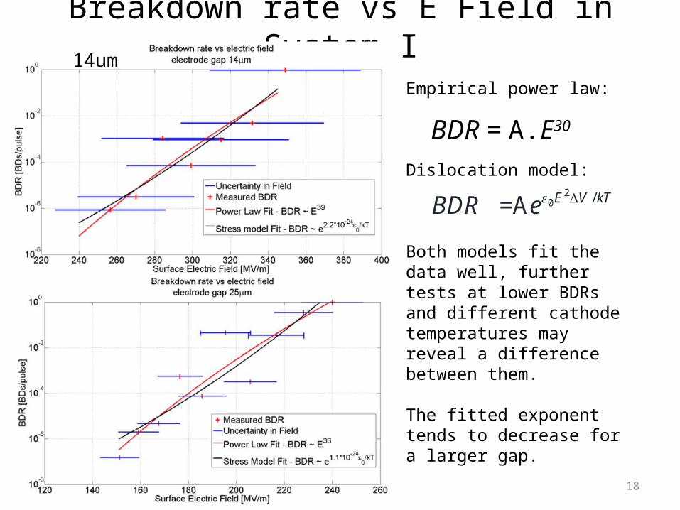
Breakdown rate vs E Field in System I14um

25um

Empirical power law:

Dislocation model:

Both models fit the data well, further tests at lower BDRs and different cathode temperatures may reveal a difference between them.

The fitted exponent tends to decrease for a larger gap.

20 / =A E V kTBDR e

BDR = A.E30

19

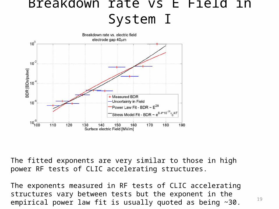
The fitted exponents are very similar to those in high power RF tests of CLIC accelerating structures.

The exponents measured in RF tests of CLIC accelerating structures vary between tests but the exponent in the empirical power law fit is usually quoted as being ~30.

Breakdown rate vs E Field in System I

20

Breakdown rate vs E Field in FGS

When conducting BDR vs E field experiments with the FGS, the breakdown rate for a given field was reduced over time.

This is known as conditioning.

It is an important an prominent effect in RF tests of accelerating structures but is not observed in System I or II due to the smaller size of the electrodes.

21

Pulse Length vs E-Field

Pulse Length

22

0 1 2 3 4 5

Pulse Length vs E-Field in System IIt was only possible to study the dependence of BDR on pulse length in System I and II and not the FGS.

The pulse lengths studied in the DC case were larger than those usually studied in RF.

The exponent in the power law fits shown here are:2.7 – for the DC case6.2 – for the RF case

23

Delay before Breakdown

24

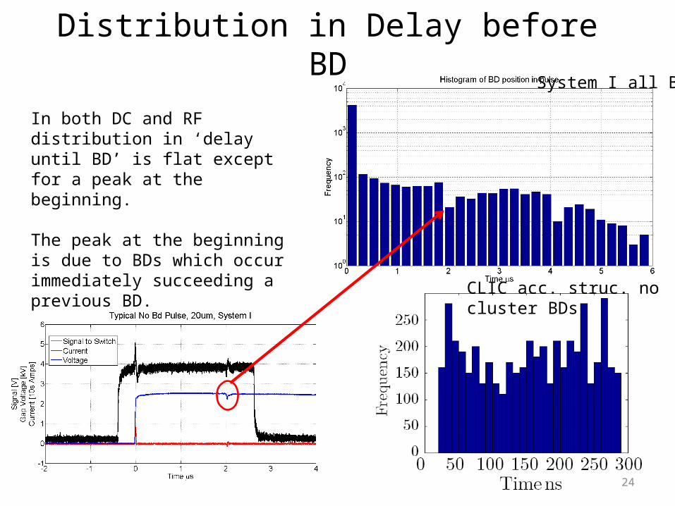
In both DC and RF distribution in ‘delay until BD’ is flat except for a peak at the beginning.

The peak at the beginning is due to BDs which occur immediately succeeding a previous BD.

Distribution in Delay before BDSystem I all BDs

CLIC acc. struc. no cluster BDs

25

Distribution in Delay before BD

The distribution in ‘delay before BD’ coupled with the pulse length dependence implies a memory effect where BDs are dependent on preceding pulses.

FGS non immediate BDs

FGS cluster BDs

26

Measured Turn on Times

27

Firstly - why are we interested in turn on time?

RF tests indicate that low group velocity, and consequently narrow bandwidth structures are able to sustain much higher surface fields than high group velocity, large bandwidth, structures.

Further study has led to the idea that the process which governs the turn on time is the instantaneous power flow available to feed the breakdown during its onset.

In other words a high group velocity structure could more quickly replenish local energy density absorbed by a growing breakdown leading to faster turn on times.

An accurate measure of the rise time of breakdowns in the DC systems under electrostatic conditions is an essential precursor to understanding whether the transient response of RF systems to the breakdown currents determine breakdown limits.

For more background see references below

[1] C. Adolphsen 2005, “Advances in Normal Conducting Accelerator Technology from the X-Band Linear Collider Program”, PAC 2005 pp.204-8. [2] A. Grudiev, S. Calatroni and W. Wuensch 2009, “New local field quantity describing the high gradient limit of accelerating structures”, PRSTAB, vol. 12, no. 10, pp.102001-1 -102001-9.

28

Turn on time measured in the DC Spark system

The turn on time appears uncorrelated with gap size or BD position, but is generally higher at higher surface fields.

29

The Swiss FEL turn on times are much longer than in the DC case and the variation is much greater, this is keeping with other RF breakdown turn on time measurements.

Comparison of turn on times

Test Measurement ResultSimulation ~0.8ns… maybeNew DC System Voltage Fall Time ~7nsTBTS (X-Band) Transmitted

Power Fall Time20-40ns

KEK (X-Band) Transmitted Power Fall Time

20-40ns

Swiss FEL (C-Band) Transmitted Power Fall Time

110-140ns

The summary table on the right suggests the characteristic size of the system breaking down may govern the turn on time.

30

Measured Burning Voltages

31

Measured Burning Voltages

Subtract average voltage with switch closed from Average voltage during breakdown after initial voltage fall.

The burning voltage was measured across here.

32

Measured Burning Voltages

Literature value Measured Value

23V 40V

Despite differences between the measured and literature value of burning voltage. The spectral power shows a 1/f^2 dependency as was also seen by Andre Anders and linked to Brownian motion of the arc foot.

33

Future Plans• Temperature dependence

• High bandwidth field emission measurements looking for pre-breakdown signals

• Further magnetic field experiments

• Local effect of electric field on BD probability

Cathode

Anode

34

Back Up Slides

35

Measured traces• Fast voltage rise, but slow voltage fall time• Pulse length adjustments not useful• Small and brief initial charging current

• The turn on time is how quickly the voltage drops after a BD.

• The BD position is the position or time the BD occurs within the pulse.

• An estimation of the burning voltage can be obtained by averaging the voltage fluctuations after the BD.

36

A cubic function is fitted to the calibration data and used to convert subsequent integral measurements to a gap distance.

Calibration Curve

How good is the measurement?

We are able to measure the gap to +-1.5um, as yet it hasn’t been determined if this is a limit on the gap measurement or the gap tends to actually vary by this amount.

The error introduced when going into contact is of the order of 1um, but this only introduces a fixed offset.

37

BD statistics at fixed voltage

38

• Bigger voltage steps more BDs per voltage level.

• Clusters mean the calculated BDR for 20 BDs may not reflect the underlying BDR.

• Gap seems to be changing once stepper motor arrives this will not be such a problem.

Total #BDs 972

Average BDR 2.95*10^-5 BDs/pulse

Std(pulses between BD) 8.54*10^4

Ratio(immediate BDs/Total BDs) 0.64

Rolling average

39

BDR Analysis of long run experiment

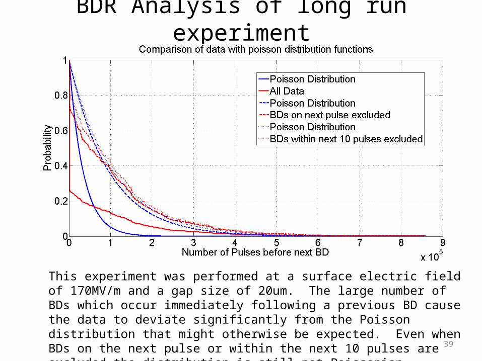
This experiment was performed at a surface electric field of 170MV/m and a gap size of 20um. The large number of BDs which occur immediately following a previous BD cause the data to deviate significantly from the Poisson distribution that might otherwise be expected. Even when BDs on the next pulse or within the next 10 pulses are excluded the distribution is still not Poissonian.

40

BD position dependenciesThe position of the BD within the pulse, in some experiments, is seen to occur later for lower fields and BDRs.

The graph below shows some old data taken at a gap of 20um but before gap monitoring was possible.

41

42

43