(SYB) 15-1

Experimental Investigation of Heat Transfer in Separated Flow on aHighly Loaded LP Turbine Cascade

Stefan Wolff, Lars Homeier, Leonhard FottnerInstitut für Strahlantriebe

Universität der Bundeswehr MünchenD-85577 Neubiberg, Germany

Stefan.Wolff@unibw-muenchen.de

ABSTRACTToday aerodynamic design tools and CFD-codes

provide excellent quality in predicting 2D and 3D flows inturbine components. Nevertheless, correlation andnumerical methods are not able to predict heat flux in asatisfactory accuracy for complex heat transfer problems,for example 3D film cooling mixing zones or areas ofseparated flow.

In order to close part of these gaps in knowledge and toimprove the understanding of the interaction between theflow pattern and the heat transfer phenomena, experimentalinvestigations were carried out focused on 2D separatedflow on the pressure side leading edge of the highly loadedlow pressure turbine cascade named T106-300.

The cascade was instrumented with pressure taps andglue-on hot-film sensors. The pressure taps provided thestatic profile pressure distribution. The hot-filmanemometry technique normally is used to detect boundarylayer development; moreover a procedure will be presentedto evaluate the heat transfer coefficient as well.Supplementary boundary layer traverses with a 1D hot-wireprobe were carried out at positions inside and downstreamof the separation.

The dimension of the separation up to 60% chord wasvaried by the incidence angle. By variation of Reynoldsnumber and Mach number a data set is available which willbe put down to a correlation.

NOMENCLATUREa [-] overheat ratioA [m2] cross-sectional areab [m] gauge width, measurement quantityd [-] incremental displacementD [m] hole diameterE [V] voltageh [W/(m2K)] heat transfer coefficientI [A] electrical currentl [m] chord lengthm, n [K/Ω], [K] coefficients of linear equation

T=ƒ(R)P [W], [-] power CTA output, probe

Q [W] heat flux

R [W] resistanceT [K] temperatureTu [%] turbulence levelU [m/s] velocityx [m] bi-tangential stream wise co-ordinateβ [°] flow angle in circumferential

directionµ3 [-] skewness, third order moment

Subscripts∞ free stream property0 zero-flow conditions1, 2 inlet / exit1..n indexing number2th exit presuming isentropic expansionc conductive, property of unheated

gaugecs cable and supporte electricfc forced convectiveL 1;2 leadsP prober radiations storaget total / stagnationw property of heated gauge

AbbreviationsBR Bridge RatioCTA Constant Temperature AnemometryD DimensionHFA Glue-On Hot-Film AnemometryHGK High-Speed Cascade Wind TunnelHTC Heat Transfer CoefficientHWA Hot-Wire AnemometryPPD Profile Pressure DistributionPS SS Pressure Side Suction SideRMS Root Mean SquareRP Reattachment PointSFC Specific Fuel ConsumptionSP Separation Point

Paper presented at the RTO AVT Symposium on “Advanced Flow Management: Part B – Heat Transfer andCooling in Propulsion and Power Systems”, held in Loen, Norway, 7-11 May 2001, and published in RTO-MP-069(I).

Report Documentation Page Form ApprovedOMB No. 0704-0188

Public reporting burden for the collection of information is estimated to average 1 hour per response, including the time for reviewing instructions, searching existing data sources, gathering andmaintaining the data needed, and completing and reviewing the collection of information. Send comments regarding this burden estimate or any other aspect of this collection of information,including suggestions for reducing this burden, to Washington Headquarters Services, Directorate for Information Operations and Reports, 1215 Jefferson Davis Highway, Suite 1204, ArlingtonVA 22202-4302. Respondents should be aware that notwithstanding any other provision of law, no person shall be subject to a penalty for failing to comply with a collection of information if itdoes not display a currently valid OMB control number.

1. REPORT DATE 00 MAR 2003

2. REPORT TYPE N/A

3. DATES COVERED -

4. TITLE AND SUBTITLE Experimental Investigation of Heat Transfer in Separated Flow on aHighly Loaded LP Turbine Cascade

5a. CONTRACT NUMBER

5b. GRANT NUMBER

5c. PROGRAM ELEMENT NUMBER

6. AUTHOR(S) 5d. PROJECT NUMBER

5e. TASK NUMBER

5f. WORK UNIT NUMBER

7. PERFORMING ORGANIZATION NAME(S) AND ADDRESS(ES) NATO Research and Technology Organisation BP 25, 7 Rue Ancelle,F-92201 Neuilly-Sue-Seine Cedex, France

8. PERFORMING ORGANIZATIONREPORT NUMBER

9. SPONSORING/MONITORING AGENCY NAME(S) AND ADDRESS(ES) 10. SPONSOR/MONITOR’S ACRONYM(S)

11. SPONSOR/MONITOR’S REPORT NUMBER(S)

12. DISTRIBUTION/AVAILABILITY STATEMENT Approved for public release, distribution unlimited

13. SUPPLEMENTARY NOTES Also see ADM001490, presented at RTO Applied Vehicle Technology Panel (AVT) Symposium held inLeon, Norway on 7-11 May 2001, The original document contains color images.

14. ABSTRACT

15. SUBJECT TERMS

16. SECURITY CLASSIFICATION OF: 17. LIMITATION OF ABSTRACT

UU

18. NUMBEROF PAGES

10

19a. NAME OFRESPONSIBLE PERSON

a. REPORT unclassified

b. ABSTRACT unclassified

c. THIS PAGE unclassified

Standard Form 298 (Rev. 8-98) Prescribed by ANSI Std Z39-18

(SYB) 15-2

INTRODUCTIONDue to the demands for more efficient gas turbine,

turbine peak cycle temperature increased rapidly in the pastenabled by an extensive use of cooling technology.Therefore a lot of research work was conducted within thisarea, since improvement in material development did notkeep up with the thermal requirements. Nevertheless, anincreasing turbine inlet temperature comes along with anincreasing cooling flow rate. Because of inappropriateaccuracy in predicting heat transfer in complex or separatedflow the safety margin in cooling design represents apotential to improve SFC.

The present work is part of the European projectAerothermal Investigation on Turbine Endwalls and Blades(AITEB) which focused on the increased ability of coolingtechnology. The aim is to enable critical parts to withstandhigher gas temperatures based on the current cooling flowrate as well as a more accurately predicted componentlifetime. This will lead to an improvement in SFC. Theobjective of the present work is the experimentalinvestigation of a huge 2D separation at the pressure sideleading edge of a low pressure turbine blade.

Several works dealt with the problem of flowseparation, reattachment and the heat transfer underseparated flow on a flat plate like Rivir [10] in addition acollection of paper published by AGARD [1]. Furthermore,a survey of literature provides some studies on morerealistic geometries like Pucher and Göhl [8] and Bellowsand Mayle [3].

The present investigation was initiated to examine theseparated, reattached flow and the interrelated heat transferat the pressure side leading edge at Mach and Reynoldsnumbers more appropriate to present low pressure turbinesand with a separation covering more then 50% chord. Forthis investigation an attempt was made to evaluate the HTCfrom measurements with heated thin-film elements. The useof glue-on hot-film sensors to investigate the heat fluximplicates a number of problems, which will be discussedin detail.

EXPERIMENTAL APPARATUS

Turbine cascadeThe experimental investigations were performed on a

large-scale plane cascade turbine model named T106-300.The cascade consists of three blades with 300 mm chordlength and two adjustable tailboards at half pitch distancefrom the upper and lower blade thus assuring flowperiodicity and high spatial resolution together with a twodimensional flow field at mid span. Measurements werecarried out exclusively on the centre blade. A sectionalsketch and the main aerodynamic and geometric design dataare given in Fig. 1.

Fig. 1 HGK test section with T106-300 cascade

High-Speed Cascade Wind TunnelThe experiments were carried out at the High-Speed

Cascade Wind Tunnel of the Universität der BundeswehrMünchen (Fig. 2). This wind tunnel is an open loop facilitywhich can operate continuously and reach Mach numbersup to Ma = 1.05 in the test section. Being built inside a largepressurised tank the wind tunnel offers the possibility tovary independently the Mach and the Reynolds number inorder to simulate flow conditions, which are typical inmodern gas turbines. The total temperature in the settlingchamber is set to 303 K. A turbulence generator upstream ofthe nozzle can adjust the turbulence intensity. The testsection exit plane inclination and height can be adjust inorder to vary the inlet flow angle. A detailed description ofthe facility is given in Sturm and Fottner [12].

Instrumentation of the test sectionTotal temperature (Tt1), total pressure (pt1) and static

pressure (p1) in front of the cascade are used for thedetermination of the inlet flow conditions. The totaltemperature data is gained in the settling chamber of thewind tunnel (Fig. 2). The static and total pressure ismeasured 96 mm upstream of the cascade inlet plane. Thetank pressure (pK) is used as reference for all other pressuremeasurements and characterizes the exit flow conditions.

4000

mm

11800 m mPressurized Tank

Plane CascadeTurbulence G enerator

Se ttling Cham berM ain Coo ler

D iffusor Axia l Com pressor(6 Stages)

G ear

HydraulicCoupling

M otor

Chord Length: 300 mmBlade Height: 300 mmPitch Ratio: 0.799Stagger Angle: 59.28°Ma1 0.28Ma2th 0.59Re2th 500000β1 127.70°β2 26.70°

(SYB) 15-3

Main test section data:

Mach Number: 0.2 ≤ Ma ≤ 1.05

Reynolds Number: 0.2 ⋅106 m-1 ≤ Re/L ≤ 16.0 ⋅106 m-1

Inlet Turbulence Level: 0.4% ≤ Tu1 ≤ 7.5%

Inlet Flow Angle: 25° ≤ β1 ≤ 155°

Test Section Width: 300 mm

Test Section Height: 235 mm ... 500 mm

Fig. 2 High-Speed Cascade Wind Tunnel

Instrumentation of the test bladeThe loading of the cascade is determined by means of

static pressure taps in the mid span section of the blade.Altogether 71 pressure taps (PS 24; SS 47) were installed atmid-span. Due to the fact that the centre blade could beexchanged, a second blade was instrumented with an arrayof 68 MTU hot-film gauges which where embedded (glue-on) into the pressure side surface. The array covered theentire pressure side at mid-span.

Fig. 3 HWA data acquisition system

Hot-Wire Anemometry (HWA)The PC based HWA data acquisition system (Fig. 3) is

controlled by the in-house developed software WINSMASH(Wolff [13]). The boundary layer measurements wereconducted using a 1D-HWA probe (DANTEC HW-55P15).For each position the probes were calibrated for the localstatic pressure. The turbulence level in the test section wasdetermined 500 mm upstream of the cascade inlet planeusing a hot-film probe (DANTEC HF-55R01). A 4th orderpolynomial has been used for the approximation of thecalibration curve.

The HWA signals were low-pass filtered with a cut offrequency of 10kHz. The mean value for a quantity b isgiven by:

∑=

=N

0jjb

N

1b (1)

where N is the number of samples and b represents thevelocity for each sample. The standard deviation of thevelocity is calculated using the RMS deviation given by:

∑=

−−

=N

0j

2j )bb(

1N

1RMS (2)

The turbulence level is normalized by the velocitycascade inlet plane U1:

%100*U

RMSTu

1

= (3)

Glue-On Hot-Film Anemometry (HFA)The HFA technique is well established to investigate

boundary layer development (e.g. Bellhouse and Schultz[2]). Furthermore, this work is an attempt to evaluate theHTC from the hot-film data. Therefore the hot-film dataacquisition system of the Institut für Strahlantriebe (Fig. 4)(Brunner et al. [4]) was adapted and employed.

Fig. 4 Layout of the data acquisition system

Two racks of the DANTEC Streamline anemometersystem, each consisting of 6 anemometers, have beenemployed. Therefore simultaneous data acquisition of 12hot-film gauges has been possible. A 12-bit A/D boardacquires up to 16 channels simultaneously. The set-up datafor each gauge is stored in a project file and is available forfurther evaluation.

The HFA data are also evaluated with equation 1 and 2where b represents the anemometer output voltage E. As anadditional value the skewness is given as the third ordermoment:

( )∑=

−⋅−

⋅=N

1jj

3

33 bb1N

1

b

1(t) (4)

(SYB) 15-4

Evaluation of Heat Transfer CoefficientThe HFA as well as the HWA is based on the

convective heat transfer from the heated sensing elementplaced in a fluid flow.

dx

Tt , G

T =t , C

Tt , G

Ta T

W

Qe

Qc

Qf c

Fig. 5 Heat-rate balance of a glue-on hot-filmsensor

The forced convective heat flux fcQ can be determined

from the heat-rate balance (Fig. 5) equation (cf. Bruun [5])for an incremental heated film element:

rQdsQdcQdfcQdeQd +++= (5)

In order to eliminate the terms of radiation, conductive andstorage heat flux, a measurement is conducted under zeroflow conditions at the same overheat ratio:

0 s;Qd0 r;Qd0 c;Qd fc;0

Qd0 e;Qd +++= (6)

Consider that:

sQd0 s;Qd;rQd0 r;Qd;cQd0 c;Qd

0fc;0

Qd

===

=(7)

The forced convective heat flux is determined as:

e;0Qd eQdfc

Qd −= (8)

The forced convective heat flux can be expressed as well interms of the HTC h:

)dxcTw(Tbdhfc

Qd −= (9)

Assuming that h is constant in x-direction, fcQ results in:

)cTw(TAhfc

Q −= (10)

The heat generation rate by an electrical current I of the hot-film with a resistance Rw given by:

wR

2wE

wR IeQ == (11)

R1

R3

R2

ERL 1

Ew

K a p to n L a y er

RL 2

I

Rw

Fig. 6 Schematic of CTA Wheatstone bridgewith hot-film

The voltage drop over the gauge can be determined bythe Kirchhoff´s laws for the electric cycle of the gauge armshown in Fig. 6:

EL2RwRL1R1R

wRwE

+++= (12)

where E is the bridge output voltage.The fixed resistance R1 and the bridge ratio BR=R2/R1

is given by the vendor of the anemometer system. Todetermine the leads resistance of the connecting flags andwires from the gauges to the CTA input RL1 and RL2, one ofthe gauges is connected with two leads on both connectingflags. This electric cycle can be used as a shorting probe.

However, it is not possible to measure the resistance ofthe heated gauge Rw under operating conditions, but theresistance can be determined considering the bridge set-upprocedure:1. Measuring the cold resistance of the probe RP at Tc

2. Calculating the cold resistance of the gauge bysubtracting the resistance of the connecting wires

L2R-

L1R-PR

cR = (13)

3. Calculating the hot resistance of the gauge by settingthe overheat ratio a:

cR a)(1wR += (14)

4. Calculating the overheat resistance of the probe

L2RL1RwRwP,R ++= (15)

5. Setting the decade resistance R3 of the adjust arm of thebridge by the bridge ratio BR:

wP,R BR3R = (16)

(SYB) 15-5

For CTA mode Rw is kept constant when the bridge isin balance. The same set-up procedure is done for the zeroflow measurement.

Using equation 4, 6 and 7 the HTC h can be calculatedas:

)T-w

A(T

1

hw,0,R

2w,0E

-

hw,R

2wE

h

∞=

(17)

The driving temperature difference is defined as thedifference between the heated gauge under flow conditionsTw and the free stream temperature T∞. The free streamtemperature is calculated using the profile pressuredistribution and the total temperature determined in thesettling chamber.

The temperature of the heated gauge can be determinedby calibrating the temperature sensitivity of the gaugeresistance. Therefore the instrumented blade was subjectedto five different temperatures and the resistance of eachgauge was measured and tabled. The resistant was found tobe linear in the range of temperatures. Related to thiscalibration measurement the temperature of the gauge canbe calculated as:

ncR a)(1 mnwR mwT ++=+= (18)

Where m, n are the linear coefficients determined bythe calibration measurement.

It should be noted, that there are several aspects, thathave to be considered using heated thin-films to determinethe HTC. First of all, the heated element represents a localstep in the wall temperature, which implicates as well a stepon the HTC (cf. Heselhaus [7]). Work is going on in orderto find a solution by superposing this problem with astandard flat plate with a wall temperature step in order tocorrect the HTC to get an adequate engineering accuracy(cf. Reynolds et al [9]). Some of the assumption that wasmade to evaluate the HTC has to be reconsidered. The mainproblem arises with the assumption in equation (7) that theheat conduction into the blade material is constant.Haselbach [6] dealt with heat balance and the calibration ofheated thin-films for skin friction measurements. Hepointed out that a part of the conductive heat loss convectsindirectly into the flow via the substrate. He stated that thisprocess is coupled with the flow conditions, which alsoaffects the effective wetted area of heat exchange. Work isgoing on for this problem in order to examine carefully theeffects on the present results respectively to find a way toeliminate this interaction.

EXPERIMENTAL RESULTSThe experiments were conducted for different inflow

conditions listed in Tab. 1. The numbers inside the bracketsare the number of boundary layer traverses.

β1 = 127.7° β1 = 105.0° β1 = 90.0°

Re2th = 150000Ma2th = 0.5

PPD, HFA,HWA (5)

PPD, HFA,HWA (7)

PPD, HFA,HWA (6)

Re2th = 200000Ma2th = 0.5

PPD, HFA,HWA (6)

Re2th = 500000Ma2th = 0.59

PPD, HFA

Tab. 1. Test program

The turbulence level in the test section upstream of thecascade inlet plane was determined to be Tu1 = 3.4% forRe2th = 150000 and Tu1 = 3.6% for Re2th = 200000.

For the discussion of the results a definition of theseparation and reattachment point is necessary. Theseparation and the reattachment point are defined as a pointof singularity, where the sign of velocity near to the wallchanges.

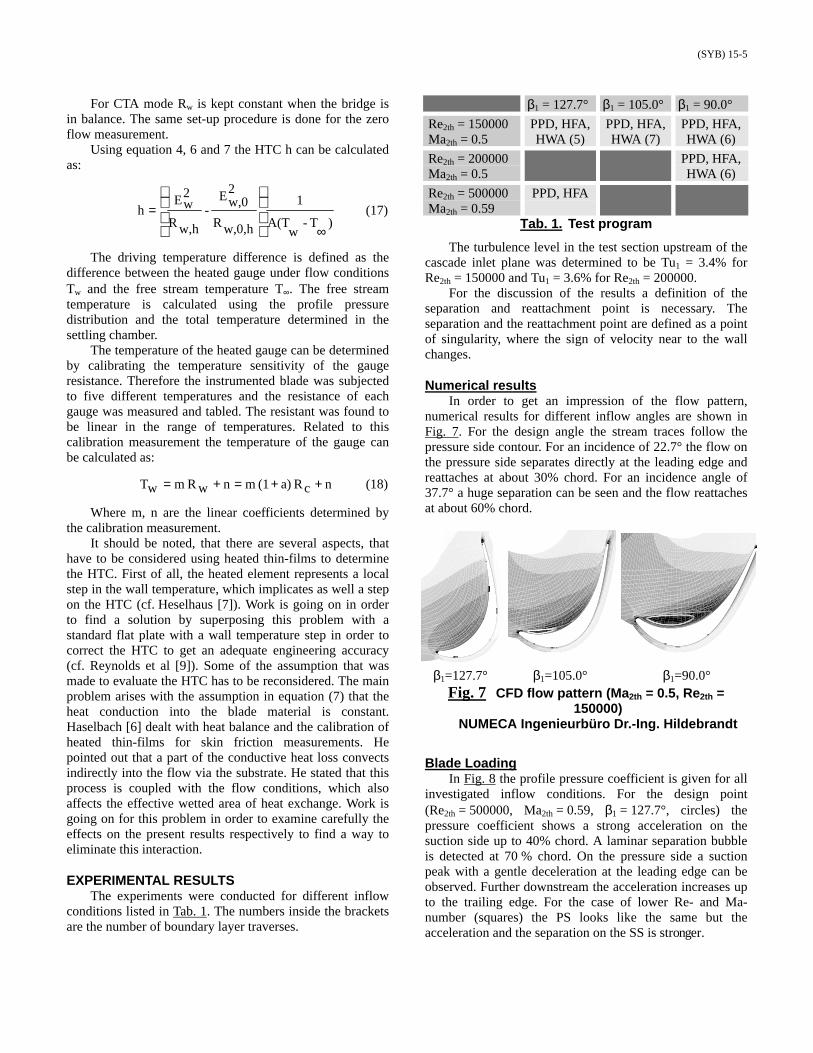
Numerical resultsIn order to get an impression of the flow pattern,

numerical results for different inflow angles are shown inFig. 7. For the design angle the stream traces follow thepressure side contour. For an incidence of 22.7° the flow onthe pressure side separates directly at the leading edge andreattaches at about 30% chord. For an incidence angle of37.7° a huge separation can be seen and the flow reattachesat about 60% chord.

β1=127.7° β1=105.0° β1=90.0°Fig. 7 CFD flow pattern (Ma2th = 0.5, Re2th =

150000)NUMECA Ingenieurbüro Dr.-Ing. Hildebrandt

Blade LoadingIn Fig. 8 the profile pressure coefficient is given for all

investigated inflow conditions. For the design point(Re2th = 500000, Ma2th = 0.59, β1 = 127.7°, circles) thepressure coefficient shows a strong acceleration on thesuction side up to 40% chord. A laminar separation bubbleis detected at 70 % chord. On the pressure side a suctionpeak with a gentle deceleration at the leading edge can beobserved. Further downstream the acceleration increases upto the trailing edge. For the case of lower Re- and Ma-number (squares) the PS looks like the same but theacceleration and the separation on the SS is stronger.

(SYB) 15-6

0.00 0.25 0.50 0.75 1.00x/l [-]

-0.4

-0.2

0.0

0.2

0.4

0.6

0.8

1.0

c p,2t

h[

-]

β1=90,0° Re=150000β1=90.0° Re=200000β1=105.0° Re=150000β1=127.7° Re=150000β1=127.7° Re=500000

Fig. 8 Profile pressure coefficient

0 0.25 0.5 0.75 1

x/l [ - ]

-0.6

-0.5

-0.4

-0.3

-0.2

-0.1

0

0.1

0.2

0.3

0.4

0.5

0.6

0.7

0.8

0.9

1

1.1

c p,2t

h[

-]

0.00 0.25 0.50 0.75x/l [-]

0.6

0.7

0.8

0.9

1.0

1.1

c p,2t

h[

-]

RP

SP

RP0.01

0.03

0.590.32

β1=90,0° Re=150000β1=105.0° Re=150000β1=127.7° Re=150000

Fig. 9 Detection of the reattachment point

In order to detect the Separation Point (SP) and theReattachment Point (RP) a zoom on the PS pressurecoefficient is shown in Fig. 9. The SP is defined as thebeginning of the area of zero pressure gradient. The RP isdefined as the intersection of the tangent originated at theSP to the graph. For β1 = 90° the SP is located at x/l = 0.03and the RP at x/l = 0.59. For β1 = 105° the flow separatesnearly at the same position whereas the separation is farsmaller with the RP at x/l = 0.32. For the variation of theRe-number for β1 = 90° no influence was detected.

Taking into account that it is problematically todetermine the RP only with the pressure coefficientdistribution, a look at other measurement results will help tovalidate the statements.

HWA ResultsIn order to get useful results the axial positions of the

HWA measurements were defined after detecting thedimension of the separation. Therefore velocity andturbulence profiles inside the separation, in the vicinity of

the reattachment as well as for the reattached boundarylayer are provided. The velocity and turbulence vectors (thetraverses are perpendicular to the surface) represent theabsolute value turned into surface tangential direction.

In Fig. 11 and Fig. 12 the velocity profiles are given forβ1 = 105.0° and β1 = 90.0° at Ma2th = 0.5, Re2th = 150000. Itshould be noted that a single hot-wire cannot by itself sensethe direction of the flow, therefore the velocity data in theseparation were plotted as measured. One might expect thatthe absolute value of the velocity converge zero in thecentre of the separation. But behaviour like this was notdetected and there are two possible reasons for that. First ofall the accuracy of the calibration for such low velocities ata static pressure level of about 5000 Pa is not reasonable.On the other hand, a separation is an unsteady phenomenaand it should be impossible to detect the streamline of zerovelocity inside the separation. For β1 = 105.0° the velocityprofiles up to x/l = 0.25 shows a region of ‘reverse’ flow.The boundary layer reattaches between x/l = 0.25 andx/l = 0.35 and the profile at x/l = 0.35 is characteristic forreattached boundary layers. The profiles furtherdownstream show the characteristics of an attachedaccelerated boundary layer.

The profiles for β1 = 90.0° (Fig. 12) indicate a farbigger separation. The profile at x/l = 0.18 shows a localminimum which denotes the middle of the separation withthe change in velocity direction. Closer to the wall thereverse flow velocity accelerates to a local maximum anddecelerates again closer to the wall. The same profilepatterns can be detected for x/l = 0.35 but the localminimum shifted closer to the wall. Somewhere betweenx/l = 0.55 and x/l = 0.60 the flow reattaches and furtherdownstream at x/l = 0.68 an attached profile was detected.

The corresponding turbulence profiles are displayed inFig. 14 and Fig. 15. Within the undisturbed channel flow theturbulence level was determined between 4% and 5%. It isvisible that the maximum level of turbulence was detectedat the border of the separation. Especially for β1 = 105° atx/l = 0.05 (Fig. 14) the peak in this region stands out clearly.Further downstream the gradient in surface normal directiondecreases. But the turbulence seems to be transportedthrough the channel. The turbulence production of the shearlayers due to the separation are dominating so that a normaldistribution with a maximum directly at the wall cannot befound until x/l = 0.55. For β1 = 90° the distributions aresimilar.

(SYB) 15-7

50 m/s

0.15

x/l = 0.05

0.35

0.45

0.55

Fig. 10 HWA velocity profiles: ββββ1 = 127.7°

50 m/s

0.18x/l = 0.050.25

0.35

0.45

0.50

0.55

Fig. 11 HWA velocity profiles: ββββ1 = 105.0°

50 m/s

x/l = 0.18

0.45

0.55

0.60

0.68

0.35

Fig. 12 HWA velocity profiles: ββββ1 = 90.0°

25 %

0.15

x/l = 0.05

0.35

0.45

0.55

Fig. 13 HWA turbulence profiles: ββββ1 = 127.7°

25 %

0.18x/l = 0.050.25

0.35

0.45

0.50

0.55

Fig. 14 HWA turbulence profiles: ββββ1 = 105.0°

25 %

x/l = 0.18

0.45

0.55

0.60

0.68

0.35

Fig. 15 HWA turbulence profiles: ββββ1 = 90.0°

(SYB) 15-8

0.0 0.2 0.4 0.6 0.8 1.0x/l [-]

0.010

0.020

0.030

(E-E

0)/E

0[-

]

β= 90.0° Re2th=150000β=105.0° Re2th=150000β=127.7° Re2th=150000

0.0 0.2 0.4 0.6 0.8 1.0x/l [-]

2.0

4.0

6.0

RM

S/E

0[1

0-4

]

0.0 0.2 0.4 0.6 0.8 1.0x/l [-]

0.0

0.5

1.0

1.5

Ske

wne

ss[-

]

Fig. 16 HFA results of boundary layer conditionsfor Re2th = 150000, Ma2th = 0.5

HFA resultsThe HFA results are predestined to detect flow

phenomena like separation and transition (e.g. Schröder etal. [11], Bellhouse et al. [2]). However, not all of theirguidelines to discuss the results are valid for pressure sideseparated flow, too. In order to detect the reattachmentlocation the quasi wall shear stresses, the dimensionless

RMS value and the skewness for Re2th = 150000 aredisplayed in Fig. 16.

For β1 = 90° a local minimum for the quasi wall shearstress and the RMS value is detected at x/l = 0.59 andindicates the reattachment point. The same pattern can beobserved for β1 = 105° at x/l = 0.32. Downstream ofx/l = 0.5 for β1 = 105° and x/l = 0.7 for β1 = 90° the valuesof wall shear stress are the same as for the design angle. Atthese positions the profile pressure distributions convergesas well.

The RMS values for the separated flow are muchhigher than for the attached flow. A gentle increase in RMSvalue for the design angle was detected downstream of thesuction peak due to the adverse pressure gradient. Furtherdownstream the value decreases continuously. For the otherangles the RMS value increases inside the separation to amaximum close to the reattachment location. A second peakin RMS values can be observed downstream of thereattachment due to the transportation of the shear layerturbulence closer to the wall. When the flow accelerates theRMS level decreases rapidly. It has to be stated that theRMS level for the cases with separated flow close to thetrailing edge is higher than for the case of attached flow.

The absolute maximum of the skewness for both offdesign angles was detected almost at the reattachment pointjust shifted slightly upstream. The zero crossing of theskewness for both off design angles coincidences with thepoint where the flow is accelerated again (e.g. Fig. 9) andthe quasi wall shear stresses converges the distribution forthe design angle.

Preliminary heat transfer resultsThe results for the local HTC are displayed in Fig. 17.

In the first figure the HTC for β1 = 90° is compared toβ1 = 127.7°. For both angles the HTC reaches the minimumat x/l = 0.05. For β1 = 127.7° a local maximum is detectedjust downstream of the suction peak and the HTC increasesrapidly when the flow is accelerated. The heat transfer forthe separated flow comes to a maximum in the middle ofthe separation and to a local minimum at the reattachmentpoint. However, the HTC for the separated flow is in thesame order than for the attached flow and at thereattachment point it is even less. For the smaller separation(β1 = 105°) the HTC shows a local maximum in the middleof the separation and a local minimum at the reattachmentpoint, too. Furthermore, a small peak was detected justdownstream of the reattachment location due to the highturbulent shear layers transported closer to the wall.Between the reattachment and the point where the profilepressure distributions converge (0.3 ≤ x/l ≤ 0.5) the HTC forthe case with separation is lower than for the design case.

CONCLUSIONA separation which covers 30% respectively 60%

chord at the leading edge pressure side of a highly loaded

(SYB) 15-9

low pressure turbine cascade was generated by a largeincidence. The boundary layer was investigated usingstandard pressure taps and 1D HWA as well as glue-on hot-film sensors for appropriate Mach and Reynolds numbers.Furthermore, a proposal was presented to evaluate HTCfrom heated thin-film measurements and specific problemswere discussed. The detected HTC increases inside theseparation with a, unlike to previous studies, local minimumin the reattachment region. The HTC for the separated andreattached flow was determined not to be higher as for thedesign angle.

0.0 0.2 0.4 0.6 0.8 1.0x/l [-]

100

200

300

400

h[W

/(m

2 K)]

β= 90.0° Re2th=150000β=127.7° Re2th=150000

0.0 0.2 0.4 0.6 0.8 1.0x/l [-]

100

200

300

400

h[W

/(m

2 K)]

β=105.0° Re2th=150000β=127.7° Re2th=150000

Fig. 17 Local HTC

ACKNOWLEDGMENTSThe reported work was performed within a research

project that is part of the European project AerothermalInvestigation on Turbine Endwalls and Blades (AITEB –Contract - Number: G4RD-CT-1999-00055). Thepermission for publication is gratefully acknowledged. Theauthor gratefully acknowledges as well the CFD support byNUMECA Ingeneurbüro Dr.-Ing. Thomas Hildebrandt asthe experimental work by Lt. Dipl.-Ing. Matthias Klein.

REFERENCES1. AGARD, 1976, “Flow Separation”, AGARD-CP-1682. Bellhouse, B.J., Schultz, D.L. 1966, “Determination of

mean and dynamic skin friction, separation andtransition in low-speed flow with a thin-film heatedelement“, J. of Fluid Mech. 1966 Vol. 24

3. Bellows, W.J., Mayle, R.E, 1986, “Heat TransferDownstream of a Leading Edge Separation Bubble“,ASME 86-GT-59

4. Brunner, S., Teusch, R., Stadtmüller, P., Fottner, L.,1998, “The Use of Simultaneous Surface Hot FilmAnemometry to Investigate Unsteady Wake InducedTransition in Turbine and Compressor Cascades“, 14th

Symposium on Measuring Techniques5. Bruun, H., 1995, “Hot-Wire Anemometry: Principles

and Signal Analysis“, Oxford University Press6. Haselbach, F., 1997, “Thermalhaushalt und Kalibration

von Oberflächenheißfilmen und Heißfilmarrays“,Fortschritt-Berichte VDI: Reihe 7 Nr. 326

7. Heselhaus, A., 1997, “Ein hybrides Verfahren zurgekoppelten Berechnung von Heißgasströmung undMaterialtemperaturen am Beispiel gekühlterTurbinenschaufeln“, Doctoral Thesis Rur-UniversitätBochum

8. Pucher, P., Göhl., R., 1986, “Experimental Investigationof Boundary Layer Separation with Heated Thin-FilmSensors”, ASME 86-GT-254

9. Reynolds, W.C., Kays, W.M., Kline, S.J., 1958, “HeatTransfer in the turbulent incompressible BoundaryLayer: III – Arbitrary Wall Temperature and HeatFlux”, NASA Memorandum 12-3-58W

10. Rivir, R.B., Johnston, J.P., Eaton, J.K., 1992, “HeatTransfer on a Flat Surface Under a Region of TurbulentSeparation”, ASME 92-GT-198

11. Schröder, T., Haueisen, V., Hennecke, D., 1998,“Measurements with Surface Mounted Hot-FilmSensors on Boundary Layer Transition in WakeDisturbed Flow”, AGARD CP-598, Nr. 38

12. Sturm, W., Fottner , L., 1985, “The High-SpeedCascade Wind Tunnel of the German Armed ForcesUniversity Munich“, 8th Symposium on MeasuringTechniques in Transonic and Supersonic Flows inCascades and Turbomachines

13. Wolff, S., 1999, “Konzeption, Programmierung undErprobung eines PC-gesteuerten Meßsystems zurAufnahme und Auswertung von 1-D und 3-D-Hitzdraht-Signalen am Hochgeschwindigkeits-Gitterwindkanal als Ersatz des HP-Systems“, InstituteReport WOIB9909

(SYB) 15-10

Paper Number: 15

Name of Discusser: H. B.Weyer, DLR Cologne

Question:Is the conclusion correct, that hot wire anemometry (HWA) is not fully appropriate to measure the flow inside the bubble, inparticular the reattachment point?Would you believe the planar laser anemomentry would be advantageous?

Answer:The conclusion is correct and for sure a non intrusive measurement technique which is able to measure low velocities could beadvantageous. However, for LDA or L2F an optical access over the entire 300 mm chord is necessary.Nevertheless, most of the measurements has been carried out in the reattached region and in this case the HWA is anappropriate tool to get information especially on the turbulence level. Furthermore, the HWA was not mainly used to detect thereattachment point.