OREGON STATE UNIVERSITY DEPARTMENT OF CHEMISTRY EXPERIMENTAL CHEMISTRY II CH 462 & CH 462H

Experiment 1

Preparation and Characterization Of Zeolite 5A Background 2 Part A. Synthesis of Zeolite 4A and Exchange to Zeolite 5A 6

Part B. X-Ray Diffraction Analysis 8

Part C. Thermogravimetric Analysis 12

Part D. Neutron Activation Analysis 14

Part E. Sorption Analysis 20 Report Guide 25 References 27

Mar 2009 rev

2

Background This experiment will introduce some important techniques in the analysis and physical characterization of solids in the context of the study of an interesting (and, until a few decades ago, practically unknown) form of crystalline solid - zeolites. The experiment includes the synthesis of zeolite 4A and ion exchange to form zeolite 5A. The following sections will involve a study of the crystal structure by X-ray diffraction, elemental analysis using neutron activation, a surface area measurement by N2 adsorption, and a study of thermogravimetric behavior. Some excellent general references on zeolites are available, several are provided in reference 1. "Zeolite" is the generic term for solids with a structural framework that contains micropores in which small molecules (water, for example) can be reversibly incorporated. This is a relatively unusual property, as most solids are based on the close packing or near close packing of ions, which optimizes the sum of electrostatic interactions (i.e., the lattice energy) of the solid. This does not usually permit large unoccupied, or pore, volumes within the lattice. The vast majority of zeolites are based on an aluminosilicate framework, although some have been prepared with other oxide frameworks (one important example being AlPO4). About two or three dozen naturally occurring minerals are zeolites, indeed, a zeolitic deposit occurs in the McDonald forest outside Corvallis. The integrated lab has a beautiful sample collected from this site. The most widely studied natural zeolite is the cubic mineral faujasite, this contains micropores of sufficient diameter to incorporate benzene and toluene; but it is exceedingly rare in nature. Another important zeolite is the hexagonal mineral chabazite, which is more common. These and many new zeolite structures have been prepared synthetically. Several decades ago, the Linde Air Products Co., whose principal products were compressed and liquefied gases, explored the possible large-scale synthesis of chabazite for use in separating the components of air by low-temperature absorption. Attempts at laboratory synthesis yielded, instead, new zeolitic structures. One was an aluminosilicate containing sodium with an entirely new structure type, and was labeled zeolite 4A. Partial exchange of the sodium ions in zeolite 4A with calcium ions yielded a product the Linde Company called zeolite 5A. This form has slightly larger pores, and is therefore capable of absorbing not only water and other small molecules, but also straight-chain hydrocarbons. Applications: Zeolites 4A and 5A, and other synthetic zeolites, were first used as drying agents and for molecular separations; because of the latter function zeolites are commonly called “molecular sieves". Under ambient conditions these zeolites are hydrated, i.e., the micropores contain water. They can be dehydrated by heating in a process known as “activation” and the activated forms are stored under a dry atmosphere. Activated zeolites are highly efficient at absorbing water, and are excellent drying agents. Since zeolites also readily undergo cation exchange, they can be used to soften water by exchanging the Mg2+ and Ca2+ in hard water for Na+. For this reason, zeolites are incorporated into many laundry detergents. Other applications for zeolites have been developed, but the most

3

important single application is probably their use as catalysts or catalyst supports. One type of synthetic faujasite, called zeolite 13Y, can have metallic platinum, palladium, or other metals dispersed within the micropores; these materials serve as important catalysts in the petroleum industry. Processes such as hydrocracking, isomerization, and alkylation, essential to the manufacture of high-octane gasoline, all require catalysts. In fact, every drop of gasoline produced today has passed through a zeolite catalyst bed.

Structural Details:

Zeolite aluminosilicate frameworks contain both silicon and aluminum ions with tetrahedral coordination by four oxide ligands. Each oxygen ligand joins two metal cations, i.e., the structure consists of corner-sharing MO4 tetrahedra. Without aluminum, the empirical formula would be SiO2. In this case, the Si4+ cation is symmetrically balanced by the charges on its four O2- ligands. Since the O2- ligands join two tetrahedra, the 2- charge is divided between them, and each ligand contributes only a 1- charge to each tetrahedron.

For each substitution of Al3+ for Si4+, the charge imbalance results in a negative charge on the framework. This is compensated by the inclusion of additional cations, these are not part of the framework but are located within the micropores. Thus, for each Al3+ in the framework, there will be one Na+, or 1/2 Ca2+, etc. These additional cations are more weakly bound and can often be exchanged by reactions in aqueous solution. The number and variety of zeolite frameworks presents one of the classic subjects in solid-state chemistry.1

The negative framework charge caused by Al3+ substitution is acceptable to a reasonably high concentration; however, the substitution of Al3+ onto adjacent sites that would share an O2- ligand causes too great of a local charge imbalance, and is not stable. Pauling's rule of electrostatic valence can be used to understand this instability in aluminum-rich zeolites.2 Al3+ therefore cannot be substituted for more than half the Si4+, for this would require the presence of such Al-O-Al linkages. Although some zeolites have very low Al contents, many contain about 1/4 to 1/2 as much Al as Si, and zeolites 4A and 5A contain nearly equal amounts of these framework cations. A general empirical formula for an aluminosilicate zeolite is (Am+)n/m AlnSi2-nO4·xH2O. Am+

represents the exchangeable cations of charge m+. There may also be more than one type of exchangeable cation, increasing the complexity of this formula. The value of n can be no greater than 1, and x is variable from zero (for a fully activated zeolite) to a maximum that depends on the total accessible pore volume in the structure. Zeolite 4A has a nominal stoichiometry of NaAlSiO4·xH2O, with x = 0-2.3. Zeolite 5A has a nominal stoichiometry of Na1/3Ca1/3AlSiO4·xH2O, with x = 0-2.6. Zeolites 4A and 5A have cubic crystal lattices3 and share the same framework structure, with n close to 1, but the exchangeable cations are Na+ in 4A and Na+ and Ca2+in 5A. Two views of the unit cell of the crystal structure for zeolite 4A and 5A are shown in Figures 1 and 2,4 some structures can also be viewed online.5

4

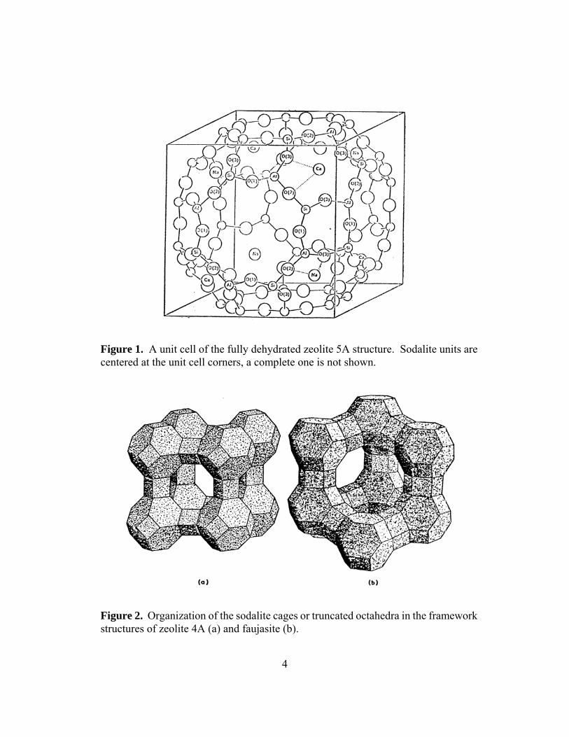
Figure 1. A unit cell of the fully dehydrated zeolite 5A structure. Sodalite units are centered at the unit cell corners, a complete one is not shown.

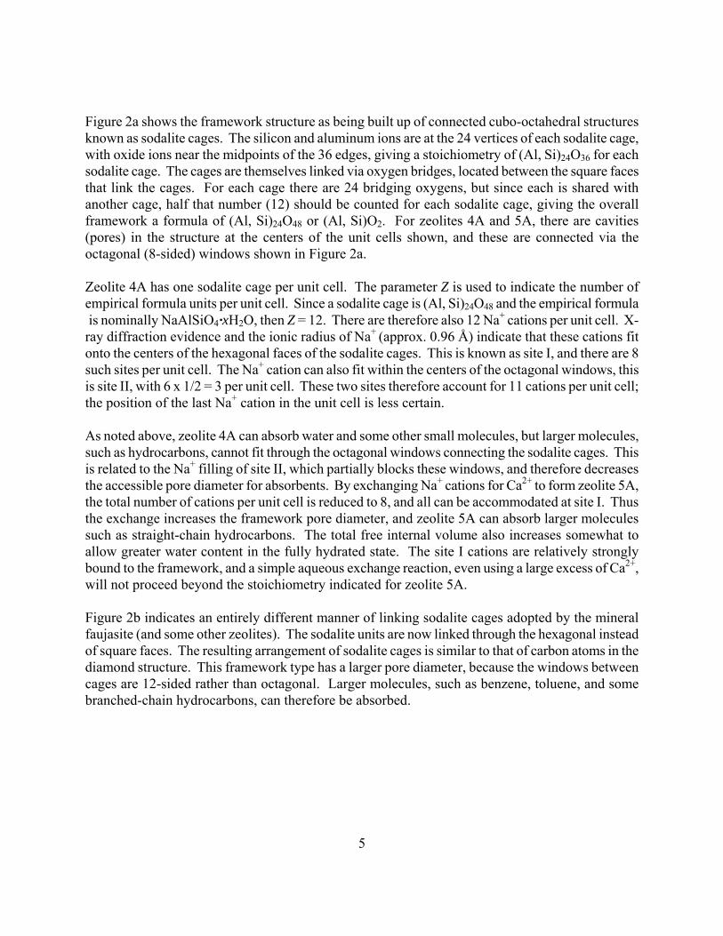
Figure 2. Organization of the sodalite cages or truncated octahedra in the framework structures of zeolite 4A (a) and faujasite (b).

5

Figure 2a shows the framework structure as being built up of connected cubo-octahedral structures known as sodalite cages. The silicon and aluminum ions are at the 24 vertices of each sodalite cage, with oxide ions near the midpoints of the 36 edges, giving a stoichiometry of (Al, Si)24O36 for each sodalite cage. The cages are themselves linked via oxygen bridges, located between the square faces that link the cages. For each cage there are 24 bridging oxygens, but since each is shared with another cage, half that number (12) should be counted for each sodalite cage, giving the overall framework a formula of (Al, Si)24O48 or (Al, Si)O2. For zeolites 4A and 5A, there are cavities (pores) in the structure at the centers of the unit cells shown, and these are connected via the octagonal (8-sided) windows shown in Figure 2a. Zeolite 4A has one sodalite cage per unit cell. The parameter Z is used to indicate the number of empirical formula units per unit cell. Since a sodalite cage is (Al, Si)24O48 and the empirical formula is nominally NaAlSiO4·xH2O, then Z = 12. There are therefore also 12 Na+ cations per unit cell. X-ray diffraction evidence and the ionic radius of Na+ (approx. 0.96 Å) indicate that these cations fit onto the centers of the hexagonal faces of the sodalite cages. This is known as site I, and there are 8 such sites per unit cell. The Na+ cation can also fit within the centers of the octagonal windows, this is site II, with 6 x 1/2 = 3 per unit cell. These two sites therefore account for 11 cations per unit cell; the position of the last Na+ cation in the unit cell is less certain. As noted above, zeolite 4A can absorb water and some other small molecules, but larger molecules, such as hydrocarbons, cannot fit through the octagonal windows connecting the sodalite cages. This is related to the Na+ filling of site II, which partially blocks these windows, and therefore decreases the accessible pore diameter for absorbents. By exchanging Na+ cations for Ca2+ to form zeolite 5A, the total number of cations per unit cell is reduced to 8, and all can be accommodated at site I. Thus the exchange increases the framework pore diameter, and zeolite 5A can absorb larger molecules such as straight-chain hydrocarbons. The total free internal volume also increases somewhat to allow greater water content in the fully hydrated state. The site I cations are relatively strongly bound to the framework, and a simple aqueous exchange reaction, even using a large excess of Ca2+, will not proceed beyond the stoichiometry indicated for zeolite 5A. Figure 2b indicates an entirely different manner of linking sodalite cages adopted by the mineral faujasite (and some other zeolites). The sodalite units are now linked through the hexagonal instead of square faces. The resulting arrangement of sodalite cages is similar to that of carbon atoms in the diamond structure. This framework type has a larger pore diameter, because the windows between cages are 12-sided rather than octagonal. Larger molecules, such as benzene, toluene, and some branched-chain hydrocarbons, can therefore be absorbed.

6

Part A. Synthesis of Zeolite 4A and Exchange to Zeolite 5A Introduction Although many early zeolite syntheses were restricted to hydrothermal methods, i.e., aqueous solutions at high temperature and pressure, zeolite 4A can be prepared from warm aqueous solutions containing silicates and aluminates combined in an appropriate stoichiometry.6 This synthesis involves a sol-gel method with a prolonged aging of the gel (usually 1 - 2 weeks) to obtain a crystalline product, therefore steps 1 - 3 below should have already been completed in advance. Experimental 1. With goggles in place, dissolve 10 g of Na2SiO3·9H2O and 10 mL of triethanolamine (TEA)

into 70 mL of distilled water and filter through a 0.45 μm filter. 2. In a separate container, dissolve 8 g of NaAlO2 · xH2O (which should be approximately 24

wt % water) and 10 mL TEA into 70 mL of distilled water and filter as above. Although zeolite 4A has an approximate 1:1 stoichiometry for Si and Al, a slight excess of Al is employed when combining reagents. Record the water content of the aluminate reagent; this will be required in later calculations.

3. In a polypropylene container, slowly stir the silicate solution into the aluminate solution then

mix well. Tightly cover the container to prevent both splattering of hot base and evaporation, and heat at 80 °C in an oven. A white gel will form, which should be aged under the same conditions at 80 °C until it cleanly segregates into a white crystalline powder and yellowish translucent overlayer, indicating the aggregation and crystallization of product. The aging period is likely to be 1 - 2 weeks.

4. Decant almost all the clear solution and then filter the solid product with a Büchner funnel. If small particles are observed in the solution overlayer, accept a slight product loss and decant the unsettled particulates prior to filtration to avoid clogging the filter paper. Wash the solid residue with distilled water until the filtrant shows a pH below 11. Rinse once with acetone or another rapidly-drying organic liquid; allow the product to air-dry, then weigh your product to ± 0.1 g to determine the reaction yield. At least 3 g of product are required for the remaining synthesis and characterization.

5. Zeolite 4A can now be converted to 5A by partial ion exchange of Na+ by Ca2+. If there is sufficient 4A product, save a portion and use only approximately 5-6 g (accurately weighed) of the 4A. Calculate the volume of 0.1 M CaCl2 required to completely exchange all of the Na+ in the 4A reagent, and add a 50 % excess of this amount to the 4A in a 500 mL beaker. Cover the beaker loosely to prevent dust or other impurities from accumulating, and slowly

7

stir the solution for at least 12 h. When stirring solutions for long unattended periods, use tape to secure the beaker to the center of the stirrer.

6. After stirring, allow the suspension to settle. Decant most of the supernatant liquid, keeping the settled solid product in the beaker. Save the decanted solution. Refill the 500 mL beaker with approximately 200 mL of deionized water, allow to settle, and decant again. Combine the decanted solution with that from the first wash. Repeat once more. Then add about 50 mL of water, stir, and pour the suspended solid into a Büchner funnel that is well-seated with a wetted # 4 Whatman (fast) filter paper. Use a wash bottle to remove nearly all the solid onto the filter, but remember that this is not quantitative gravimetric analysis.

7. Wash the solid in the funnel until the washes give a negative chloride ion test with a 0.01 M AgNO3 solution. Rinse the zeolite with acetone or other rapidly-drying organic liquid, remove from the filter paper, and air dry.

8. Discard the combined decanted solutions if at least 3 g of product are obtained. Otherwise, these solutions may be filtered in a similar manner to give a small additional yield.

9. The subsequent experiments will require either fully hydrated or dehydrated (activated) zeolite 5A samples. Place at least 1 g of the zeolite 5A product in a closed system (a metal desiccator with desiccant removed is suitable) containing a small beaker of water at ambient temperature. After 24 h, the zeolite will be assumed to have fully hydrated. A second sample containing at least 2 g should be activated at 400 °C for at least 24 h.

8

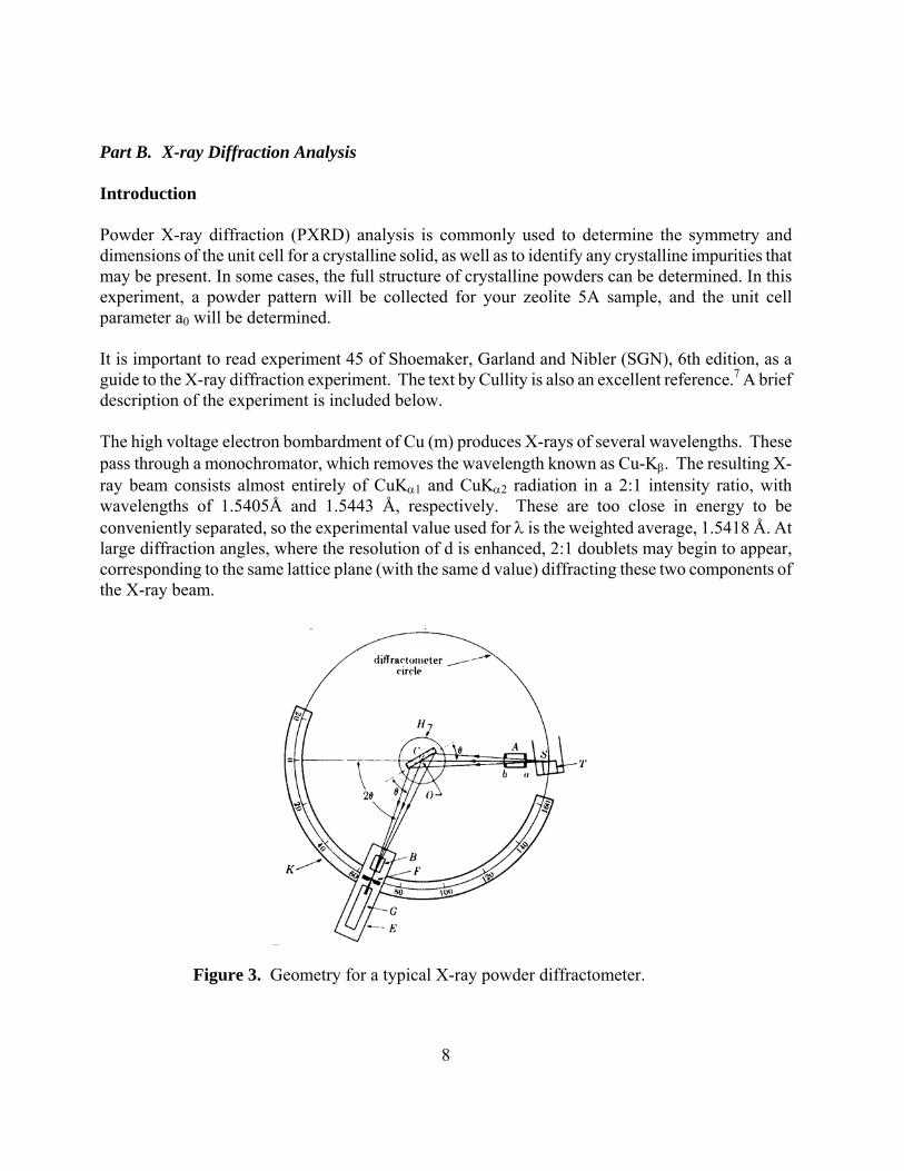
Part B. X-ray Diffraction Analysis Introduction Powder X-ray diffraction (PXRD) analysis is commonly used to determine the symmetry and dimensions of the unit cell for a crystalline solid, as well as to identify any crystalline impurities that may be present. In some cases, the full structure of crystalline powders can be determined. In this experiment, a powder pattern will be collected for your zeolite 5A sample, and the unit cell parameter a0 will be determined. It is important to read experiment 45 of Shoemaker, Garland and Nibler (SGN), 6th edition, as a guide to the X-ray diffraction experiment. The text by Cullity is also an excellent reference.7 A brief description of the experiment is included below. The high voltage electron bombardment of Cu (m) produces X-rays of several wavelengths. These pass through a monochromator, which removes the wavelength known as Cu-Kβ. The resulting X-ray beam consists almost entirely of CuKα1 and CuKα2 radiation in a 2:1 intensity ratio, with wavelengths of 1.5405Å and 1.5443 Å, respectively. These are too close in energy to be conveniently separated, so the experimental value used for λ is the weighted average, 1.5418 Å. At large diffraction angles, where the resolution of d is enhanced, 2:1 doublets may begin to appear, corresponding to the same lattice plane (with the same d value) diffracting these two components of the X-ray beam.

Figure 3. Geometry for a typical X-ray powder diffractometer.

9

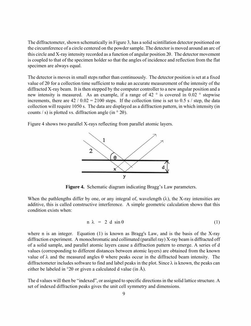
The diffractometer, shown schematically in Figure 3, has a solid scintillation detector positioned on the circumference of a circle centered on the powder sample. The detector is moved around an arc of this circle and X-ray intensity recorded as a function of angular position 2θ. The detector movement is coupled to that of the specimen holder so that the angles of incidence and reflection from the flat specimen are always equal. The detector is moves in small steps rather than continuously. The detector position is set at a fixed value of 2θ for a collection time sufficient to make an accurate measurement of the intensity of the diffracted X-ray beam. It is then stepped by the computer controller to a new angular position and a new intensity is measured. As an example, if a range of 42 ° is covered in 0.02 ° stepwise increments, there are 42 / 0.02 = 2100 steps. If the collection time is set to 0.5 s / step, the data collection will require 1050 s. The data are displayed as a diffraction pattern, in which intensity (in counts / s) is plotted vs. diffraction angle (in ° 2θ). Figure 4 shows two parallel X-rays reflecting from parallel atomic layers.

Figure 4. Schematic diagram indicating Bragg’s Law parameters.

When the pathlengths differ by one, or any integral of, wavelength (λ), the X-ray intensities are additive, this is called constructive interference. A simple geometric calculation shows that this condition exists when:

n λ = 2 d sin θ (1) where n is an integer. Equation (1) is known as Bragg's Law, and is the basis of the X-ray diffraction experiment. A monochromatic and collimated (parallel ray) X-ray beam is diffracted off of a solid sample, and parallel atomic layers cause a diffraction pattern to emerge. A series of d values (corresponding to different distances between atomic layers) are obtained from the known value of λ and the measured angles θ where peaks occur in the diffracted beam intensity. The diffractometer includes software to find and label peaks in the plot. Since λ is known, the peaks can either be labeled in °2θ or given a calculated d value (in Å). The d values will then be “indexed”, or assigned to specific directions in the solid lattice structure. A set of indexed diffraction peaks gives the unit cell symmetry and dimensions.

10

Experimental Sample Preparation: The sample powder should contain particles with dimensions < 10 μm to ensure that all diffraction planes are statistically represented, and will therefore need to be ground and sieved before loading into the XRD sample cells. 1. Grind about 0.25 g of the hydrated 5A zeolite to a fine powder in a mortar.

2. The sample should be pressed flat into the sample holder using a microscope glass slide. It is essential that the surface of the sample be flat and at the same height as the edges of the sample holder. The powder should fully pack the sample window, so that the sample fills the incident beam at all angles. Diffraction profiles are affected by surface roughness, so the sample must have a flat and smooth surface.

Use of X-ray Apparatus:

Zeolite 5A will be examined by using the Seimens D5000 powder diffractometer in Gilbert 214. Rules issued by the OSU Radiation Safety Office must be read before doing the experiment and followed exactly. All operations involving the X-ray unit must be done under the supervision of a qualified instructor. All instrument operators will wear a finger ring on one hand to assess any radiation exposure. 3. The D5000 will be programmed to collect the data from 5° – 60° 2θ, plot a diffraction

pattern of intensity vs angle, and find and label peaks with their d values (in Å). Obtain a printout of this powder diffraction pattern – include it as a figure in the report.

4. After the experiment, the sample can be discarded, the holder rinsed with distilled water and

dried with a tissue.

Data Analysis: Indexing the data obtained involves assigning the indices (hkl) to diffraction peaks to indicate the orientation of the relevant lattice planes within the structure. This will provide the unit cell parameters for the crystal structure. 5. Prepare an Excel spreadsheet with columns labeled peak number, peak intensity, and d, and

then input your data. For peak intensities, use labels very weak (VW), weak (W), medium (M), or strong (S), and add (BR) for broad peaks.

11

6. Add columns labeled M2 and a0. M2 is an integer value, starting with 1 for the first peak, that will be determined by examination of the data. Set the a0 column to calculate d * M. The a0 values should be displayed with 4 decimal places (to 0.0001 Å).

7. Starting with M2 = 1 for the first peak (which should be at about 7.21°) enter the appropriate integer values for M2 so that the calculated a0 values are consistent for each peak. Some peaks may not give reasonable a0 values for any integer assigned to M2, if so, skip them and mark as not indexed. The criterion for a reasonable value for a0 at low angle is about 0.1 Å variation from the previous value. As the diffraction angle increases this should decrease to about 0.01 Å. The decreasing variations in a0 are mainly because of the measurement of an increasing angle at a constant angular error.

8. For peaks that cannot be assigned a reasonable M2 value, recheck the diffraction pattern to see if the peaks are unusually broad, weak or asymmetric. These characteristics could cause the assigned peak position to be inaccurate. Some peaks might be reported as two or more closely spaced peaks with slightly different d values, in this case, choose only the peak with the greater intensity. Finally, some peaks might not be indexed because they are due to another (impurity) phase. In all cases, leave these peaks out of subsequent calculations of the unit cell parameter, but they should be discussed in the report.

9. The M2 used in this calculation is derived from the Miller index of the observed reflection, and for the cubic crystal system, M2 = h2 + k2 + l2. Assign integral h, k, and l values to each peak indexed with an M2 value above, and include in an extra spreadsheet column. Remember to determine out all possible combinations of h,k, and l for each case, but do not include more than one symmetry-related direction such as (100), (010), and (001). Some peaks can have more than one possible indexing, for example: M2 = 50 may be indexed as (550), (710), and (543).

10. From the eight highest-angle peaks indexed, determine the average value for a0 and the standard deviation. Report the value with the correct number of significant figures (e.g., 12.123(4) Å).

12

Part C. Thermogravimetric Analysis

Introduction Chapter 4 in “Solid State Chemistry” by West8 provides a good background for thermal analysis of solids. There is also an instruction sheet provided for the Shimadzu TGA, and more detailed information in the instrument instruction manuals. Thermogravimetric analysis (TGA) is employed to examine mass changes of a sample that arise from controlled heating or cooling. A sample is placed in an open pan on a microbalance and heated (or cooled) at a constant rate. The mass is monitored continuously and plotted against temperature. Mass changes may arise from chemical or physical reactions such as dehydration or decomposition. Some experimental parameters include the temperature range studied, the heating rate, and the atmosphere employed. Examples of atmospheres can be inert gases like He or N2, or reactive gases such as O2, air, or H2. Experimental 1. The components of the Shimadzu TGA in GbAd 314 must be turned on the following order:

(1) the TA-60WS buffer interface unit, (2) the TGA, and (3) the computer, monitor and printer. The system can be turned off in any order desired, although the computer may freeze if the interface is turned off first. The system should be turned off only if it will not be used again for more than 24 hours. We recently upgraded some components and software to the 60 series but our instrument is a 50 series so you will see both labels throughout.

3. The TGA module should already be aligned and have a clean sample chamber and Pt pan. Before proceeding, check with the instructor that this is so.

4. Turn on the N2 purge gas and check on the left side of the TGA that the gas flow rate is approximately 25 mL/min.

5. With the furnace raised into the closed (or up) position and a clean, empty sample pan in place, zero the mass reading with the balance knob. Two lights, one on each side of the zero level reading above the balance knob should be lighted after zeroing (the mass may not read exactly zero, but should be close, that’s okay, go on.)

6. Autozero the TGA by pressing the Autozero key once then press Enter. Also, set the first derivative to zero by pressing Autozero, then the down arrow key, and the press Enter.

7. Preweigh 15 ± 1 mg of hydrated zeolite 5A powder onto tare paper. Lower the furnace (down arrow), slide the protecting metal cover in place, and use a small spatula to carefully place the sample into the Pt pan. The mass added can be monitored on the digital

13

readout. Do not touch the sample pans or lids with bare hands, use the tweezers. When done, press the up arrow to raise the furnace.

8. Open the TA-60WS Collection Monitor shortcut to the program if not already open and Select TGA-50H Channel 1 for the TGA (our system is actually the model number 50 and the software will also run model 60). This will open an active window to the instrument. Under the TGA-50H menu, select Measure and Setting Parameters and setup the following temperature program which controls the temperature sequence for the furnace. Use a 10 °C/min heating rate from 25 °C to 600 °C. Press the Download button to send these new parameters from the computer to the instrument. Under File Information, enter sample information and include the sample weight, by clicking on the weight button in the menu. Enter your group name and sample name also.

When you press Start under Measure, you will be prompted for a file name otherwise the data will be written to an automatic filename using today’s date and will be stored in C:\TAData with a .tad file extension. Watch the screen until the TGA mass trace is steady and then the experiment can be started by clicking the Start button on the upper right of the screen (there are several menus that lead to “start” a run).

9. After the run is complete, open your file in the Analysis software and obtain the overall mass and the mass percent losses. If clear break points in the run are apparent from the plots, determine the mass changes within distinct regions. Double click to set the boundaries of the regions you want to analyze. Generate and print plots of both mass percent change vs. temperature and, if the data permit, a derivative curve. Derivative is found under Manipulate on the menu and you may have to smooth the derivative curve (use 200 or so points.)

10. To provide additional cooling to the furnace after the run, turn on the small plastic fan on the bench. When the TGA has cooled below 45 °C, lower the furnace, then remove, empty, and clean the pan with acetone. Replace the pan, close the furnace, and turn off the N2 flow.

14

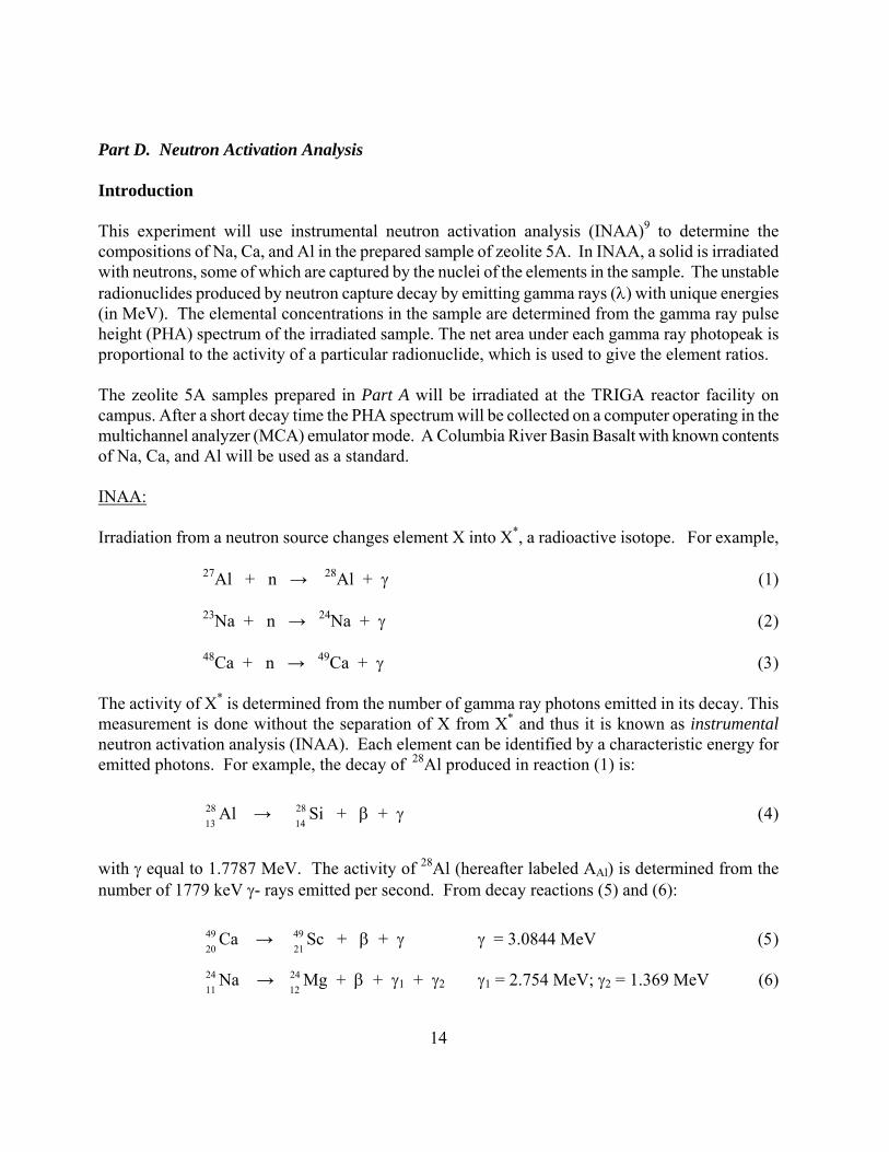
Part D. Neutron Activation Analysis Introduction This experiment will use instrumental neutron activation analysis (INAA)9 to determine the compositions of Na, Ca, and Al in the prepared sample of zeolite 5A. In INAA, a solid is irradiated with neutrons, some of which are captured by the nuclei of the elements in the sample. The unstable radionuclides produced by neutron capture decay by emitting gamma rays (λ) with unique energies (in MeV). The elemental concentrations in the sample are determined from the gamma ray pulse height (PHA) spectrum of the irradiated sample. The net area under each gamma ray photopeak is proportional to the activity of a particular radionuclide, which is used to give the element ratios.

The zeolite 5A samples prepared in Part A will be irradiated at the TRIGA reactor facility on campus. After a short decay time the PHA spectrum will be collected on a computer operating in the multichannel analyzer (MCA) emulator mode. A Columbia River Basin Basalt with known contents of Na, Ca, and Al will be used as a standard. INAA: Irradiation from a neutron source changes element X into X*, a radioactive isotope. For example,

27Al + n → 28Al + γ (1) 23Na + n → 24Na + γ (2) 48Ca + n → 49Ca + γ (3)

The activity of X* is determined from the number of gamma ray photons emitted in its decay. This measurement is done without the separation of X from X* and thus it is known as instrumental neutron activation analysis (INAA). Each element can be identified by a characteristic energy for emitted photons. For example, the decay of 28Al produced in reaction (1) is:

1328 Al →

1428 Si + β + γ (4)

with γ equal to 1.7787 MeV. The activity of 28Al (hereafter labeled AAl) is determined from the number of 1779 keV γ- rays emitted per second. From decay reactions (5) and (6):

2049 Ca →

2149 Sc + β + γ γ = 3.0844 MeV (5)

1124 Na →

1224 Mg + β + γ1 + γ2 γ1 = 2.754 MeV; γ2 = 1.369 MeV (6)

15

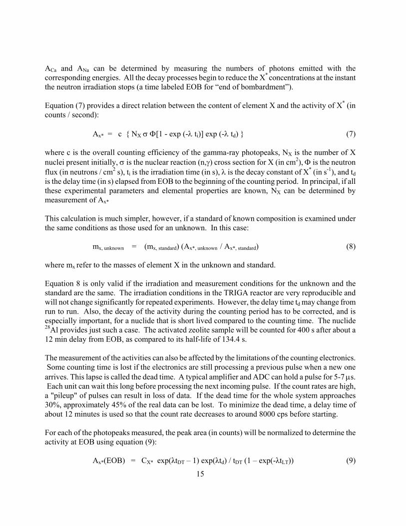
ACa and ANa can be determined by measuring the numbers of photons emitted with the corresponding energies. All the decay processes begin to reduce the X* concentrations at the instant the neutron irradiation stops (a time labeled EOB for “end of bombardment”). Equation (7) provides a direct relation between the content of element X and the activity of X* (in counts / second): Ax* = c { NX σ Φ[1 - exp (-λ ti)] exp (-λ td) } (7) where c is the overall counting efficiency of the gamma-ray photopeaks, NX is the number of X nuclei present initially, σ is the nuclear reaction (n,γ) cross section for X (in cm2), Φ is the neutron flux (in neutrons / cm2 s), ti is the irradiation time (in s), λ is the decay constant of X* (in s-1), and td is the delay time (in s) elapsed from EOB to the beginning of the counting period. In principal, if all these experimental parameters and elemental properties are known, NX can be determined by measurement of Ax* This calculation is much simpler, however, if a standard of known composition is examined under the same conditions as those used for an unknown. In this case: mx, unknown = (mx, standard) (Ax*, unknown / Ax*, standard) (8) where mx refer to the masses of element X in the unknown and standard. Equation 8 is only valid if the irradiation and measurement conditions for the unknown and the standard are the same. The irradiation conditions in the TRIGA reactor are very reproducible and will not change significantly for repeated experiments. However, the delay time td may change from run to run. Also, the decay of the activity during the counting period has to be corrected, and is especially important, for a nuclide that is short lived compared to the counting time. The nuclide 28Al provides just such a case. The activated zeolite sample will be counted for 400 s after about a 12 min delay from EOB, as compared to its half-life of 134.4 s. The measurement of the activities can also be affected by the limitations of the counting electronics. Some counting time is lost if the electronics are still processing a previous pulse when a new one arrives. This lapse is called the dead time. A typical amplifier and ADC can hold a pulse for 5-7 μs. Each unit can wait this long before processing the next incoming pulse. If the count rates are high, a "pileup" of pulses can result in loss of data. If the dead time for the whole system approaches 30%, approximately 45% of the real data can be lost. To minimize the dead time, a delay time of about 12 minutes is used so that the count rate decreases to around 8000 cps before starting. For each of the photopeaks measured, the peak area (in counts) will be normalized to determine the activity at EOB using equation (9): Ax*(EOB) = CX* exp(λtDT – 1) exp(λtd) / tDT (1 – exp(-λtLT)) (9)

16

where Ax*(EOB) is the normalized activity at EOB for X* (in counts / s), CX* is the net area of the photopeak (in counts / s), tLT is the live time (in s) that the counting system is active, and tDT is the dead time (in s). The dead time is the difference between the real clock time elapsed (tRT) and tLT. Equation 9 can be rewritten by combining all terms on the right hand side except Cx* : Ax*(EOB) = (CX*) (Fexp) (10) where the normalization factor Fexp accounts for both the differences in the delay time and dead time for different runs. Fexp can be determined for each run from the experimental parameters and eq 9. By combining eqs 8 and 10: mx,u = (mx,s) (Cx*,u / Cx*,s) (Fexp,u / Fexp,s) (11) where the u and s subscripts indicate values for unknown and standard samples. This can be rewritten as: mx,u = (mx,s) (Cx*,u / Cx*,s) (F’) (12) where F’ = Fexp,u / Fexp,s. Some additional simplifications may be possible. If the live time is the same for the sample and standard, then: F’ = [(tDT,s) (exp(λtd,u)) (exp(λtDT,u) – 1) ] / [(tDT,u) (exp(λtd,s)) (exp(λtDT,s) – 1)] (13) Moreover, if the decay time before counting (td) is maintained the same for the unknown and standard:

F’ = [ (tDT,s) (exp(λtDT,u) – 1)] / [(tDT,u) (exp(λtDT,s) – 1)] (14) Experimental Design: The unknown and standard samples should ideally have the same size, composition, and homogeneity so that decay conditions for the initial activating radiation and of the sample radiation during counting are exactly the same. This is accomplished by ensuring that both samples have the same physical volume, are irradiated in a homogeneous flux, and are counted under the same conditions (geometry, detector, etc.). Irradiation and decay conditions should be selected so that the activity of X* is enhanced relative to all other activities produced. Various activating sources (gamma rays, thermal neutrons, fast neutrons, charged particles) are available. In this experiment, the most generally useful particle is

17

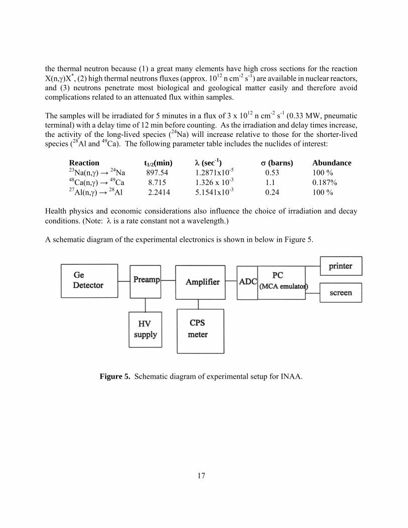
the thermal neutron because (1) a great many elements have high cross sections for the reaction X(n,γ)X*, (2) high thermal neutrons fluxes (approx. 1012 n cm-2 s-1) are available in nuclear reactors, and (3) neutrons penetrate most biological and geological matter easily and therefore avoid complications related to an attenuated flux within samples. The samples will be irradiated for 5 minutes in a flux of 3 x 1012 n cm-2 s-1 (0.33 MW, pneumatic terminal) with a delay time of 12 min before counting. As the irradiation and delay times increase, the activity of the long-lived species (24Na) will increase relative to those for the shorter-lived species (28Al and 49Ca). The following parameter table includes the nuclides of interest: Reaction t1/2(min) λ (sec-1) σ (barns) Abundance 23Na(n,γ) → 24Na 897.54 1.2871x10-5 0.53 100 % 48Ca(n,γ) → 49Ca 8.715 1.326 x 10-3 1.1 0.187% 27Al(n,γ) → 28Al 2.2414 5.1541x10-3 0.24 100 % Health physics and economic considerations also influence the choice of irradiation and decay conditions. (Note: λ is a rate constant not a wavelength.) A schematic diagram of the experimental electronics is shown in below in Figure 5.

Figure 5. Schematic diagram of experimental setup for INAA.

18

Typical pulse height spectrum for a zeolite Experimental Sample Preparation 1. The sample should be prepared the day or morning before the experiment begins. All

participants must arrive promptly at 1:00 PM at the Radiation Center.

2. Prepare a sample of hydrated zeolite 5A by quantitatively weighing 0.25 g ± 0.1 mg into a 2/5 dram polyvial. Heat-seal the vial in GBAD 309. Wear latex gloves when handling the vial and keep it in a sealed plastic bag until use.

3. Obtain the mass of the prepared standard from the instructor. According to the 1982 Consensus Values for USGS Rock Standards, CRB is known to contain at least 31 elements. For the elements of interest in the current study, it has the following composition: Al2O3, 13.63 %; CaO, 6.95%; Na2O, 3.27%.

INAA experiment: 4. Accompany the instructor to the Rabbit room, D102, and observe the irradiation procedure.

Record the following data in a lab notebook: sample name, sample mass (g), irradiation time, EOB (end of bombardment) clock time, wall monitor and cutie-pi monitor, window open and window closed.

5. Observe transfer of sample to a clean outer vial and accompany instructor to the counting lab in B100.

19

6. The instructor will place the sample on shelf positions 5 to 9, depending on the count rate. Let the sample decay for 12 minutes from EOB or until a count rate of 8,000-10,000 cps is observed on the count rate meter. Starting on the minute, count the sample for 400 s. Do a Print Screen to save a hard copy of the spectrum. Also save the pulse height spectrum to a file by transferring the contents of the MCA buffer over to the PC (ALT-5) and save as FILENAME.CHN (ALT-8). (IF THIS IS NOT DONE, ALL DATA WILL BE LOST!)

7. Repeat steps 4 – 6 for the standard.

8. Calculate tLT, tRT, and tDT for the unknown and standard.

9. Next obtain the net area (in counts) for each of the four peaks of interest. Use the F9 and F10 keys to move the cursor to the side of the first peak. Starting 3 or 4 channels to one side, continue to 3 or 4 on the other side. Press the F2 key until S is highlighted. Move the cursor to the other side of the peak and press F2 to off. Repeat for the other 3 peaks. Select "Calc" from the menu, (the "ROI area" to calculate net peak areas) and then "type" to get a hard copy.

20

Part E. Sorption Analysis

Introduction Experiment 26, Chapter XIX (Vacuum Techniques p. 615-642), and Chapter XXI (Gas Handling, p. 691-697) of Shoemaker, Garland and Nibler (SGN), 6th edition, should be read in preparation for the experiment. The specific surface area of a solid refers to its total accessible area per gram (in m2/g). For zeolites, the accessible surface include the micropores contained within the framework structure, and the area of this internal surface area far exceeds that due to the external surface of zeolite particles. Generally, the term absorb refers to incorporation into the micropores, whereas adsorb refers to binding to the external particle surface. The specific surface area can be obtained by measuring the uptake of sorbed (adsorbed and absorbed) molecules for a given quantity of solid, and converting this to a surface area from the known dimensions of the sorbant. In this experiment, N2 gas will be the sorbant used to determine the specific surface area of anhydrous zeolite 5A. When N2(g) is added to an evacuated system containing the zeolite, the amount of gas sorbed depends on the pressure and temperature. When the pressure reaches approximately a quarter to a third of the N2 vapor pressure at the system temperature, the accessible surface will be completely covered by a monolayer of N2 molecules. As the pressure approaches the vapor pressure, the amount sorbed again increases to a form a bilayer and then multi-layers of sorbent on the accessible surfaces. It is often convenient to refer to the system’s reduced pressure, which is defined as P / P0, with P0 equal to the vapor pressure of the sorbant at the sample temperature. Of course, at the vapor pressure of sorbant (when the reduced pressure equals 1), the sorbant will liquefy onto the zeolite sample (and on every other surface as well). In this experiment, an N2 monolayer will be generated on the accessible zeolite surface. How can the specific surface area be determined from the known mass and dimensions of sorbent? Consider the present example, the sorption of N2 on a zeolite. The density of liquid N2 is 0.808 g/mL. Assuming that N2 molecules are spherical, and that the bulk liquid consists of close-packed spheres (which fill 76% of space), the volume (in Å3) occupied by one N2 molecule can be determined. From this volume, the radius (in Å) and then the cross-sectional area (in Å2) of an N2 molecule can be obtained. Å3 / molecule N2 = (14.0 g / mol) (1E24 Å3 / mL) (0.76) . (0.808 g / mL N2 liq) (6.02E23 molecules / mol)

21

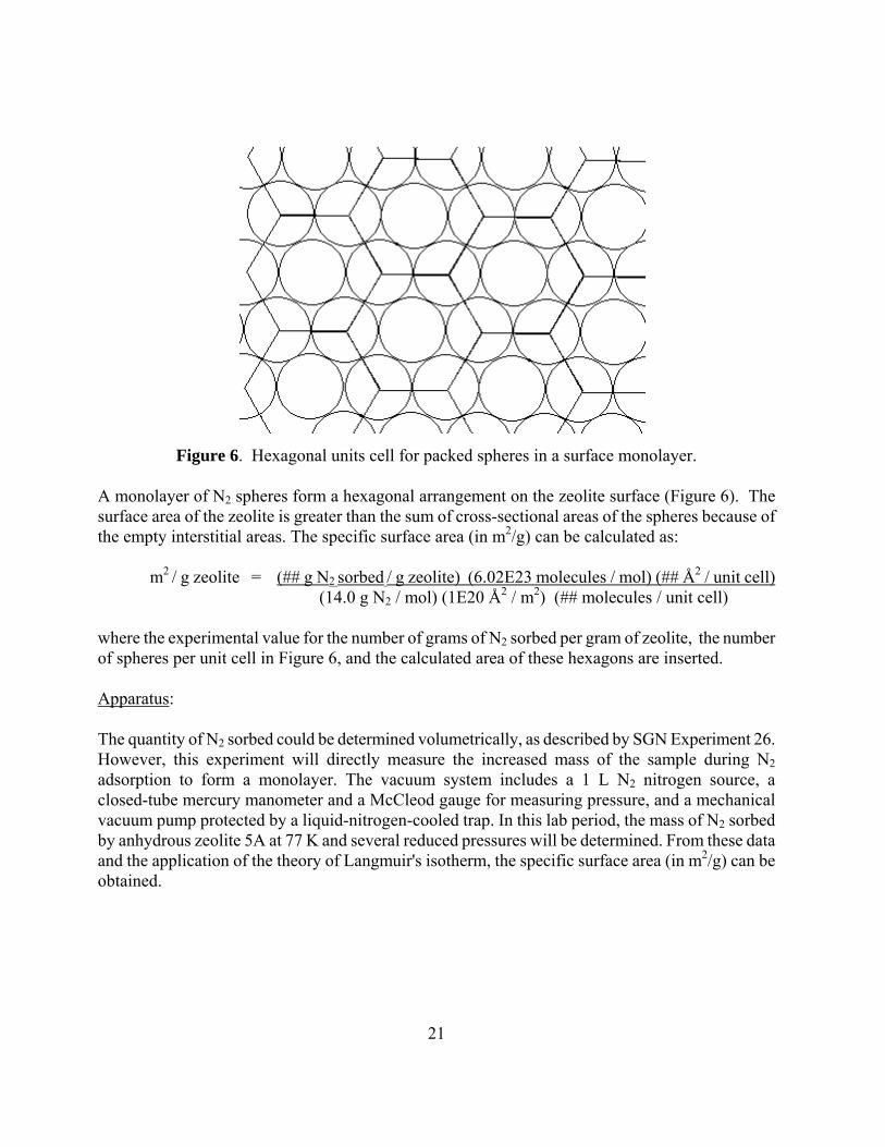
Figure 6. Hexagonal units cell for packed spheres in a surface monolayer.

A monolayer of N2 spheres form a hexagonal arrangement on the zeolite surface (Figure 6). The surface area of the zeolite is greater than the sum of cross-sectional areas of the spheres because of the empty interstitial areas. The specific surface area (in m2/g) can be calculated as: m2 / g zeolite = (## g N2 sorbed / g zeolite) (6.02E23 molecules / mol) (## Å2 / unit cell) (14.0 g N2 / mol) (1E20 Å2 / m2) (## molecules / unit cell) where the experimental value for the number of grams of N2 sorbed per gram of zeolite, the number of spheres per unit cell in Figure 6, and the calculated area of these hexagons are inserted. Apparatus: The quantity of N2 sorbed could be determined volumetrically, as described by SGN Experiment 26. However, this experiment will directly measure the increased mass of the sample during N2 adsorption to form a monolayer. The vacuum system includes a 1 L N2 nitrogen source, a closed-tube mercury manometer and a McCleod gauge for measuring pressure, and a mechanical vacuum pump protected by a liquid-nitrogen-cooled trap. In this lab period, the mass of N2 sorbed by anhydrous zeolite 5A at 77 K and several reduced pressures will be determined. From these data and the application of the theory of Langmuir's isotherm, the specific surface area (in m2/g) can be obtained.

22

Experimental Note: The instructor will explain the use of the vacuum line and related apparatus before running the experiment. 1. Remove the anhydrous zeolite sample from the 400°C oven (use caution when handling),

place into a desiccator, close, and allow it to cool to ambient temperature. 2. Record the atmospheric pressure with the manometer.

3. Making certain that the evacuated sections are closed off from air and the manometer, turn on the mechanical pump. Place a Dewar flask around the cold trap protecting the vacuum pump and fill with liquid nitrogen. Slowly open the manometer to vacuum and establish that the line pressure is < 5 torr. Use the McLeod gauge for pressures less than 5 torr. Open connections to test the entire vacuum line. If the pressure is not < 100 μm within 5 minutes, there is probably a leak in the system.

4. Remove the Al bucket from the hook and accurately obtain its mass to 0.1 mg.

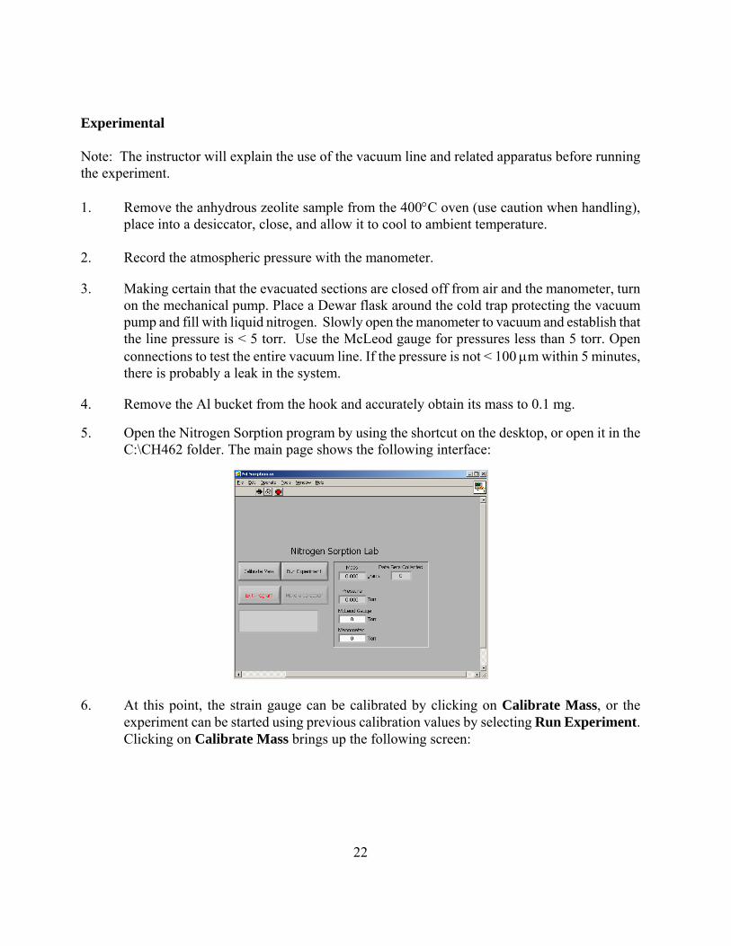
5. Open the Nitrogen Sorption program by using the shortcut on the desktop, or open it in the C:\CH462 folder. The main page shows the following interface:

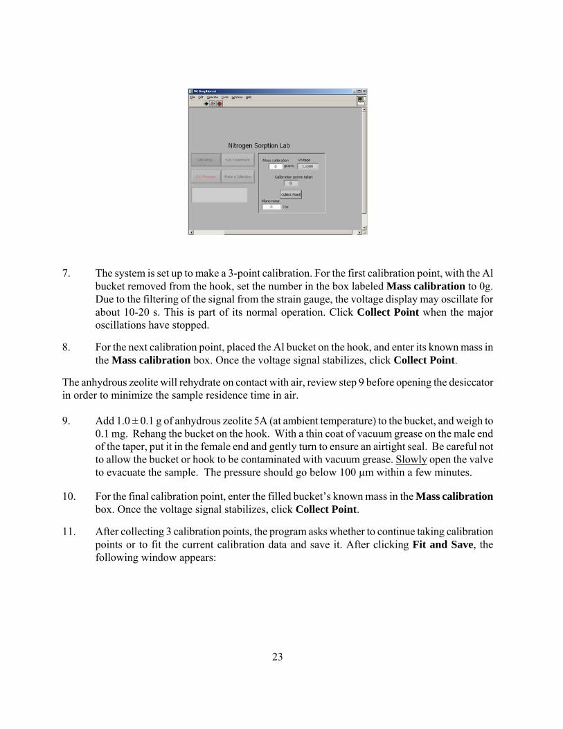
6.  At this point, the strain gauge can be calibrated by clicking on Calibrate Mass, or the experiment can be started using previous calibration values by selecting Run Experiment. Clicking on Calibrate Mass brings up the following screen:

23

7. The system is set up to make a 3-point calibration. For the first calibration point, with the Al bucket removed from the hook, set the number in the box labeled Mass calibration to 0g. Due to the filtering of the signal from the strain gauge, the voltage display may oscillate for about 10-20 s. This is part of its normal operation. Click Collect Point when the major oscillations have stopped.

8. For the next calibration point, placed the Al bucket on the hook, and enter its known mass in the Mass calibration box. Once the voltage signal stabilizes, click Collect Point.

The anhydrous zeolite will rehydrate on contact with air, review step 9 before opening the desiccator in order to minimize the sample residence time in air. 9. Add 1.0 ± 0.1 g of anhydrous zeolite 5A (at ambient temperature) to the bucket, and weigh to

0.1 mg. Rehang the bucket on the hook. With a thin coat of vacuum grease on the male end of the taper, put it in the female end and gently turn to ensure an airtight seal. Be careful not to allow the bucket or hook to be contaminated with vacuum grease. Slowly open the valve to evacuate the sample. The pressure should go below 100 µm within a few minutes.

10. For the final calibration point, enter the filled bucket’s known mass in the Mass calibration box. Once the voltage signal stabilizes, click Collect Point.

11. After collecting 3 calibration points, the program asks whether to continue taking calibration points or to fit the current calibration data and save it. After clicking Fit and Save, the following window appears:

24

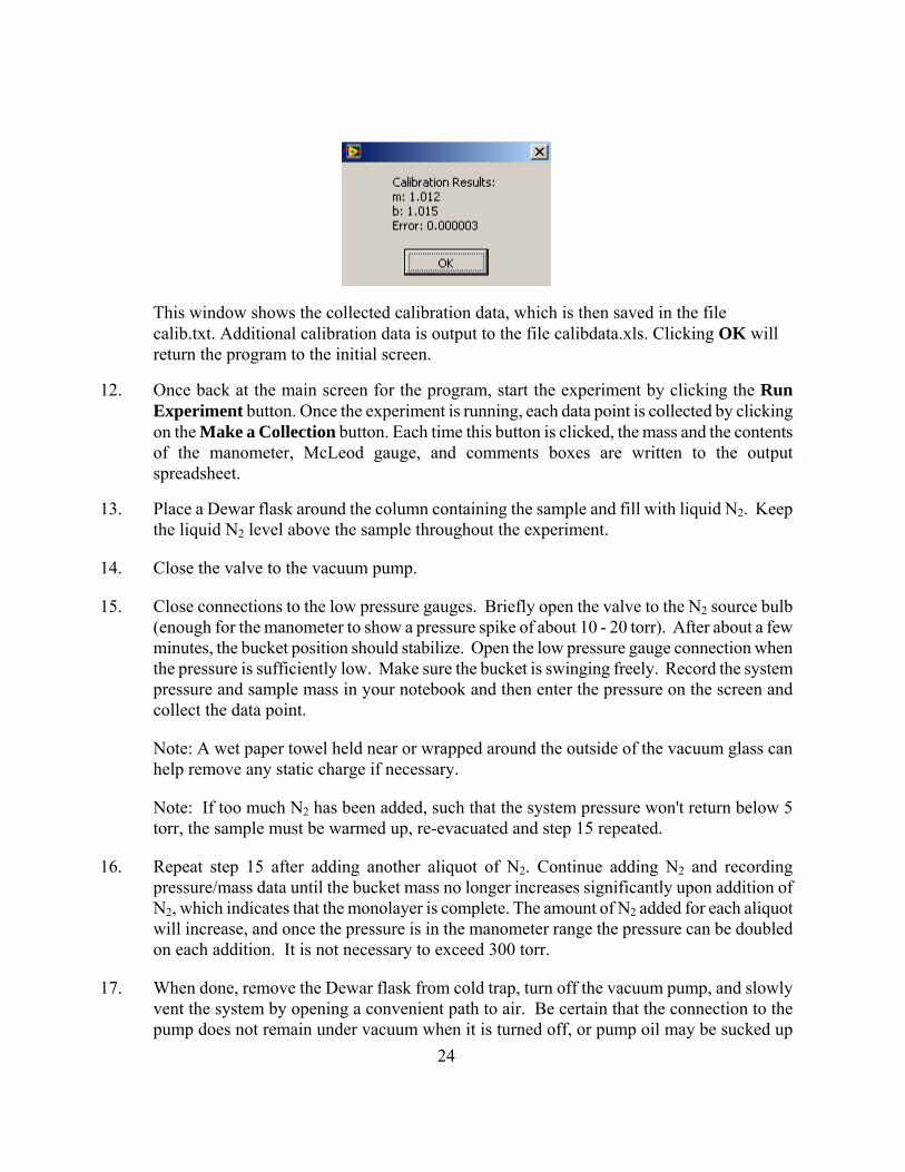
This window shows the collected calibration data, which is then saved in the file calib.txt. Additional calibration data is output to the file calibdata.xls. Clicking OK will return the program to the initial screen.

12. Once back at the main screen for the program, start the experiment by clicking the Run Experiment button. Once the experiment is running, each data point is collected by clicking on the Make a Collection button. Each time this button is clicked, the mass and the contents of the manometer, McLeod gauge, and comments boxes are written to the output spreadsheet.

13. Place a Dewar flask around the column containing the sample and fill with liquid N2. Keep the liquid N2 level above the sample throughout the experiment.

14. Close the valve to the vacuum pump.

15. Close connections to the low pressure gauges. Briefly open the valve to the N2 source bulb (enough for the manometer to show a pressure spike of about 10 - 20 torr). After about a few minutes, the bucket position should stabilize. Open the low pressure gauge connection when the pressure is sufficiently low. Make sure the bucket is swinging freely. Record the system pressure and sample mass in your notebook and then enter the pressure on the screen and collect the data point.

Note: A wet paper towel held near or wrapped around the outside of the vacuum glass can help remove any static charge if necessary.

Note: If too much N2 has been added, such that the system pressure won't return below 5 torr, the sample must be warmed up, re-evacuated and step 15 repeated.

16. Repeat step 15 after adding another aliquot of N2. Continue adding N2 and recording pressure/mass data until the bucket mass no longer increases significantly upon addition of N2, which indicates that the monolayer is complete. The amount of N2 added for each aliquot will increase, and once the pressure is in the manometer range the pressure can be doubled on each addition. It is not necessary to exceed 300 torr.

17. When done, remove the Dewar flask from cold trap, turn off the vacuum pump, and slowly vent the system by opening a convenient path to air. Be certain that the connection to the pump does not remain under vacuum when it is turned off, or pump oil may be sucked up

25

into the vacuum line. Dispose of your sample and clean out the bucket with methanol for reuse. Clean any stray grease near the sample position glass column assembly.

Report Guide:

Appendices should include:

1. Calculation of the limiting reagents, and theoretical, and percent yields for the two syntheses.

2. Calculation of Fexp for Ca, Al, and Na for the zeolite and standard runs. For Na, do separate calculations for both photopeaks. Be careful of time units (e.g., if λ is expressed in terms of min-1, then times must be expressed in minutes).

3. Calculation of the masses of Na, Ca, and Al in the standard (use at least 3 decimal places for each atomic mass) and in the zeolite. For Na, do a separate calculation for each peak and average the results. Also calculate the estimated error in the masses using σ from the printout, a sample mass error of 0.28 mg, and equation (8).

4. Calculation of the mass percents of Na, Ca, Al, Si, and water in the product. The mass percent of water will be from the TGA results. Assume that the zeolite is composed of only the elements Na, Ca, Al, Si, O, and water, and that the mole ratio of Si:Al is 1:1.

Results section should include:

1. Reactions for the preparation of zeolite 4A and 5A and the percent yields of both products.

2. The X-ray diffraction pattern for zeolite 5A. As with all figures or tables, this figure should have a number and title according to the ACS format.

3. The table generated to index the diffraction pattern.

4. The unit cell symmetry - primitive (P), face centered (F) or body centered (I) cubic, and the unit cell parameter a0.

5. A figure showing the TGA plot of mass percent vs. temperature. Temperatures of maximum loss rate, and the final mass loss, should be reported.

6. The pulse height spectrum, the summary of the net peak areas, and the parameter table (e.g., sample mass and times).

7. A table containing the raw data obtained in step 4 and the calculated parameters from step 8 in the INAA experiment.

26

8. A table containing net peak areas and calculated standard deviations for Ca, Al, and Na for the zeolite and the standard (these are indicated on the hardcopy), and the calculated F factor for each run.

9. A table containing the mass of Na, Ca, Al, Si and water per gram of zeolite, and the estimated errors in these values. From the mass percents, give the empirical formula for the product assuming 4 oxygen atoms per formula unit.

10. The density of hydrated zeolite 5A (in g/cm3) determined from a0, Z, and the empirical formula weight. From this density calculation, also report the volumetric water capacity of zeolite (in g of water/cm3 of solid).

11. A table containing the sorption data; N2 pressure, reduced pressure, sample mass, and total g N2 sorbed.

12. A Langmuir isotherm showing sorbed mass of N2 plotted against P/P0.

13. The specific surface area of zeolite 5A.

Discussion section should include: 1. How does the a0 value obtained compare with that reported in reference 3? Are these values

within the reported standard deviations? 2. Were any impurities detected in the sample?

3. How do the experimental and nominal stoichiometries compare? What is the significance of any differences?

4. Is the calculated empirical formula charge balanced? If not, what does this mean? How do the assumptions in the calculations (Si:Al ratio and the elements present) affect your conclusions?

5. Zeolites are good absorbents for small molecules and ions. How does the volumetric density of water in hydrated zeolite 5A compare with that in other hydrates?

6. Do any features in the TGA trace indicate the nature of the water bonding within the zeolite?

27

References 1. Some general references for zeolites include (a) Breck, D. W. Zeolite Molecular Sieves:

Structure, Chemistry and Use; Wiley & Sons: New York, 1974.; (b) Breck, D. J. Chem. Ed. 1964, 41, 678; Barrer, R.M. J. Incl. Phenom. 1983, 1, 105; (c) Ozin, G.W. et. al. Adv. Mater. 1989, 101, 373.

2. Pauling, L. The Nature of the Chemical Bond, 3rd ed.; Cornell University Press: Ithaca, NY,

1960, pp. 547ff. 3. Broussard, L.; Shoemaker, D.P. J. Am. Chem. Soc. 1960, 82, 1041. 4. Reproduced from Seff, K.; Shoemaker, D.P. Acta Cryst. 1967, 22, 162. 5. See http://www.iza-structure.org/databases/. These web pages are based on the data gathered

by the authors of the Atlas for Zeolite Structure Types. (accessed 12/15/2004). 6. Adapted from Charnell, J. J. Cryst. Growth 1971, 8, 291. 7. Cullity, B. D. Elements of X-Ray Diffraction, 2nd ed.; Addison-Wesley: Reading, MA, 1978. 8. West, A. R. W. Solid State Chemistry and its Applications; Wiley & Sons: New York, 1984;

Chapter 4. 9. Wang, C. H.; Willis, D. L.; Loveland, W. D. Radiotracer Methodology in the Biological,

Environmental, and Physical Sciences; Prentice-Hall: New York, 1975.