Example of applying GAM: Articulographyjvanrij/LSA2015/sheets.pdf · Example of applying GAM:...

Example of applying GAM: Articulography

Martijn Wieling and Jacolien van Rij

University of Groningen/Tübingen

LSA Institute 2015, Chicago, July 7

1 | Martijn Wieling and Jacolien van Rij - Articulography University of Groningen/Tübingen

This lectureI Introduction

I ArticulographyI Using articulography to study L2 pronunciation differences

I Design

I Methods: R code

I Results

I Discussion


Articulography


Obtaining data


Recorded data


Study setup: differences between native andnon-native English

I 19 native Dutch speakers from GroningenI 22 native Southern Standard British English speakers from London

I Material:I 10 minimal pairs [t]:[T] repeated twice:

I ‘fate’-‘faith’, ‘forth’-‘fort’, ‘kit’-‘kith’, ‘mitt’-‘myth’, ‘tent’-‘tenth’I ‘tank’-‘thank’, ‘team’-‘theme’, ‘tick’-‘thick’, ‘ties’-‘thighs’, ‘tongs’-‘thongs’I Note that the sound [T] does not exist in the Dutch languageI The pronunciation of the words was preceded and followed by /@/

I Goal: compare distinctions between both sound contrasts for both groups


Data overview> load('art.rda')

> head(art)

Word Axis Sensor Participant RecBlock@_faith_@ X TB VENI-EN_1 6@_faith_@ X TB VENI-EN_1 6@_faith_@ X TB VENI-EN_1 6@_faith_@ X TB VENI-EN_1 6@_faith_@ X TB VENI-EN_1 6@_faith_@ X TB VENI-EN_1 6

Time.normWord SeqNr Position.norm Sound Group0.002777711 21 84.22126 TH EN0.010648939 21 84.40235 TH EN0.018520166 21 84.30614 TH EN0.026391394 21 84.23431 TH EN0.034262621 21 84.19509 TH EN0.042133849 21 83.93635 TH EN

> dim(art)[1] 342850 10


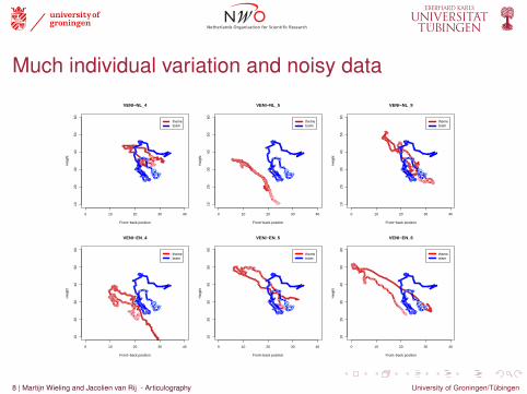
Much individual variation and noisy data

●●●●●●

●●●●

●●●

●●

●●●●●

●●●

● ●●

● ●●●●●

●●

● ●●

●●●

●●●

●●●●●●●●●●

●●●●●

●● ●

● ●● ● ●●●●●●●

●●●●●●

●●●

● ●●●

●●

0 10 20 30 40

1020

3040

5060

VENI−NL_4

Front−back position

Hei

ght

●

●

●●●

●●●

●●●

●●●●●

●●●●●●●

●

● ●

●●

●

●

●

● ●

●

●

●●●●●●●●

●●●

●● ●

●

●

●●

●● ●● ●●

● ●●

●

●●

●●

● ●●●

●●●●●●●

●●●●●●

themeteam

●●●●●●●●●●●●●●●●●●●●●●●●●●●●●●●●●●●●●

●●●●●●

●●●●●●

●●●●

●

●●●

●●●

●●●●●●●●●●●●●●●● ●●●

●●●●●

●

●●●●●●●●●

●●●●

●●●●●●● ●●●●

● ●●●●●●●

●●● ●

●●●●

●●●●●

●●●●●●●●

●●●●●●●●●●●●●●●●●●●●

●●●●●●●●●●●●●●● ●

0 10 20 30 40

1020

3040

5060

VENI−NL_5


Hei

ght

●

●

●●●

●●●

●●●

●●●●●

●●●●●●●

●

● ●

●●

●

●

●

● ●

●

●

●●●●●●●●

●●●

●● ●

●

●

●●

●● ●● ●●

● ●●

●

●●

●●

● ●●●

●●●●●●●

●●●●●●

themeteam

●●●

●●●●●

●●●

●●●●●●●●●●

●● ●●

●●●●●

●●

●●

●

●

●

●

●●

●●●●

●●●

●●

●

●

●

●●●●●●●●

●●●●

●●●

●●●●

●

●●

●

●

●

●

●●

● ●●

●●●

●●●●●●●●●●●●

●●●

●●●●●●●●●

●●●●●●●●●●●●●●●

0 10 20 30 40

1020

3040

5060

VENI−NL_9


Hei

ght

●

●

●●●

●●●

●●●

●●●●●

●●●●●●●

●

● ●

●●

●

●

●

● ●

●

●

●●●●●●●●

●●●

●● ●

●

●

●●

●● ●● ●●

● ●●

●

●●

●●

● ●●●

●●●●●●●

●●●●●●

themeteam

●●

●●●●

●●

●●

●

●●●

●●

●

●●●

●●●●

●●●

●●●●●●●●●

●●●

●●●●●●●

●●●

●●●●●

●●●●

●●●●●●●

●

●●●

● ●●

●●●●●●●

●●●●

●●●●●●●●●●

●●

●

●● ●

● ●●

● ●●●

●●●●●●●●● ●

●●●●

●●●●●●

●●●●●●●●●●

●

●

●

0 10 20 30 40

1020

3040

5060

VENI−EN_4


Hei

ght

●

●

●●●

●●●

●●●

●●●●●

●●●●●●●

●

● ●

●●

●

●

●

● ●

●

●

●●●●●●●●

●●●

●● ●

●

●

●●

●● ●● ●●

● ●●

●

●●

●●

● ●●●

●●●●●●●

●●●●●●

themeteam

● ●●●

●●

●●●

●●●●

●● ●●

●●

●●

●●

●●●●●

●●●

● ●●

●●●●●●

●●●● ●●●

●● ●●●

● ●

●

●

●●

●

●

●

●

●

●● ●●●

●●●

●●● ●●●●●●

0 10 20 30 40

1020

3040

5060

VENI−EN_5


Hei

ght

●

●

●●●

●●●

●●●

●●●●●

●●●●●●●

●

● ●

●●

●

●

●

● ●

●

●

●●●●●●●●

●●●

●● ●

●

●

●●

●● ●● ●●

● ●●

●

●●

●●

● ●●●

●●●●●●●

●●●●●●

themeteam

●●

●●●●●●●●●●●

●●●●

●●●

●

●●

●

●

●

●

●

●

●●●●●●●

●●●●●●●●●●●●●

●

●

●●●

●●●

●●●●●●●

●●●●

● ●●

●●●

●●

●●

●●

●●●

●●●●●●●●●●●

●●●●●●●●

0 10 20 30 40

1020

3040

5060

VENI−EN_6


Hei

ght

●

●

●●●

●●●

●●●

●●●●●

●●●●●●●

●

● ●

●●

●

●

●

● ●

●

●

●●●●●●●●

●●●

●● ●

●

●

●●

●● ●● ●●

● ●●

●

●●

●●

● ●●●

●●●●●●●

●●●●●●

themeteam


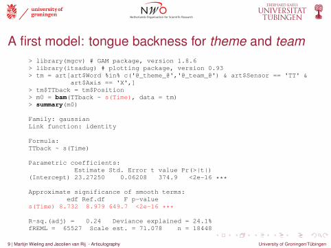
A first model: tongue backness for theme and team> library(mgcv) # GAM package, version 1.8.6> library(itsadug) # plotting package, version 0.93> tm = art[art$Word %in% c('@_theme_@','@_team_@') & art$Sensor == 'TT' &

art$Axis == 'X',]> tm$TTback = tm$Position> m0 = bam(TTback ~ s(Time), data = tm)> summary(m0)

Family: gaussianLink function: identity

Formula:TTback ~ s(Time)

Parametric coefficients:Estimate Std. Error t value Pr(>|t|)

(Intercept) 23.27250 0.06208 374.9 <2e-16 ***

Approximate significance of smooth terms:edf Ref.df F p-value

s(Time) 8.732 8.979 649.7 <2e-16 ***

R-sq.(adj) = 0.24 Deviance explained = 24.1%fREML = 65527 Scale est. = 71.078 n = 18448


Visualizing the non-linear time pattern of the model(Interpreting GAM results always involves visualization)

> par(mfrow=c(1,2)) # 2 plots in one window> plot(m0, rug=F, shade=T, main='Partial effect', ylab='TTback')> plot_smooth(m0, view='Time', rug=F, main='Full effect')

0.0 0.2 0.4 0.6 0.8 1.0

−6

−4

−2

02

46

Partial effect

Time

TT

back

0.0 0.2 0.4 0.6 0.8 1.0

1820

2224

2628

30

Full effect

Time

TT

back


Check for additional wigglyness(if p-value is low and edf close to k’)

> gam.check(m0)

Method: fREML Optimizer: perf newtonfull convergence after 10 iterations.Gradient range [-9.676733e-06,8.869831e-06](score 65527.35 & scale 71.07836).Hessian positive definite, eigenvalue range [3.770432,9223.002].Model rank = 10 / 10

Basis dimension (k) checking results. Low p-value (k-index<1) mayindicate that k is too low, especially if edf is close to k'.

k' edf k-index p-values(Time) 9.000 8.732 0.999 0.45


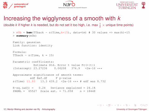
Increasing the wigglyness of a smooth with k(double k if higher k is needed, but do not set it too high, i.e. max 1

2 × unique time points)

> m0b = bam(TTback ~ s(Time,k=15), data=tm) # 30 values => max(k)=15> summary(m0b)

Family: gaussianLink function: identity

Formula:TTback ~ s(Time, k = 15)


(Intercept) 23.27236 0.06208 374.9 <2e-16 ***


s(Time) 11.93 13.3 439.2 <2e-16 *** # edf was 8.732



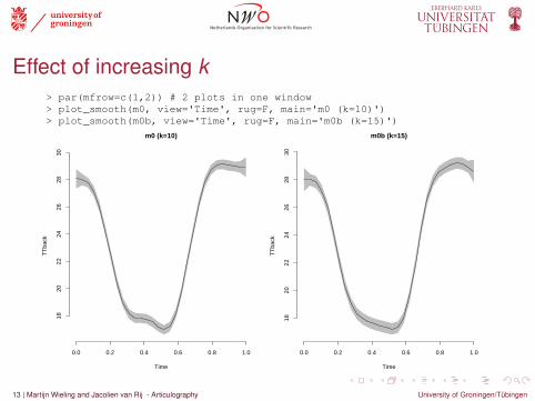
Effect of increasing k> par(mfrow=c(1,2)) # 2 plots in one window> plot_smooth(m0, view='Time', rug=F, main='m0 (k=10)')> plot_smooth(m0b, view='Time', rug=F, main='m0b (k=15)')

0.0 0.2 0.4 0.6 0.8 1.0

1820

2224

2628

30

m0 (k=10)

Time

TT

back

0.0 0.2 0.4 0.6 0.8 1.0

1820

2224

2628

30

m0b (k=15)

Time

TT

back


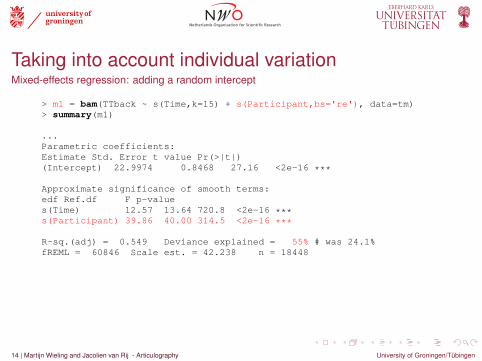
Taking into account individual variationMixed-effects regression: adding a random intercept

> m1 = bam(TTback ~ s(Time,k=15) + s(Participant,bs='re'), data=tm)> summary(m1)

...Parametric coefficients:Estimate Std. Error t value Pr(>|t|)(Intercept) 22.9974 0.8468 27.16 <2e-16 ***

Approximate significance of smooth terms:edf Ref.df F p-values(Time) 12.57 13.64 720.8 <2e-16 ***s(Participant) 39.86 40.00 314.5 <2e-16 ***

R-sq.(adj) = 0.549 Deviance explained = 55% # was 24.1%fREML = 60846 Scale est. = 42.238 n = 18448


Effect of including a random intercept> par(mfrow=c(1,2)) # 2 plots in one window> plot_smooth(m0b, view='Time', rug=F, main='m0b')> plot_smooth(m1, view='Time', rug=F, main='m1', rm.ranef=T)

0.0 0.2 0.4 0.6 0.8 1.0

1820

2224

2628

30

m0b

Time

TT

back

0.0 0.2 0.4 0.6 0.8 1.0

1520

2530

m1

Time

TT

back


Taking into account individual variationMixed-effects regression: adding a random slope

> m2 = bam(TTback ~ s(Time,k=15) + s(Participant,bs='re') +s(Participant,Time,bs='re'), data=tm)

> summary(m2)

...Parametric coefficients:

Estimate Std. Error t value Pr(>|t|)(Intercept) 22.9984 0.9461 24.31 <2e-16 ***


s(Time) 12.66 13.69 718.9 <2e-16 ***s(Participant) 39.42 40.00 44340.0 <2e-16 ***s(Participant,Time) 39.15 40.00 37387.2 <2e-16 ***

R-sq.(adj) = 0.59 Deviance explained = 59.2% # was 55%fREML = 60043 Scale est. = 38.394 n = 18448


Effect of including a random slope> par(mfrow=c(1,2)) # 2 plots in one window> plot_smooth(m1, view='Time', rug=F, main='m1', rm.ranef=T)> plot_smooth(m2, view='Time', rug=F, main='m2', rm.ranef=T)

0.0 0.2 0.4 0.6 0.8 1.0

1520

2530

m1

Time

TT

back

0.0 0.2 0.4 0.6 0.8 1.0

1520

2530

m2

Time

TT

back


Taking into account individual variationAdding a non-linear random effect

I The effect of time is non-linear and may vary non-linearly per subjectI We need a random intercept/slope which is non-linear

I (instead of random intercept and random slope of time per subject)

> m3 = bam(TTback ~ s(Time,k=15) + s(Time,Participant,bs='fs',m=1), data=tm)> summary(m3)


Estimate Std. Error t value Pr(>|t|)(Intercept) 23.05 1.16 19.86 <2e-16 ***


s(Time) 12.4 13.34 28.55 <2e-16 ***s(Time,Participant) 318.6 368.00 68.22 <2e-16 ***

R-sq.(adj) = 0.678 Deviance explained = 68.4% # was 59.2%fREML = 58146 Scale est. = 30.087 n = 18448


Visualization of individual variation> plot(m3, select=2)

0.0 0.2 0.4 0.6 0.8 1.0

−10

010

20

Time

s(T

ime,

Par

ticip

ant,3

18.5

6)


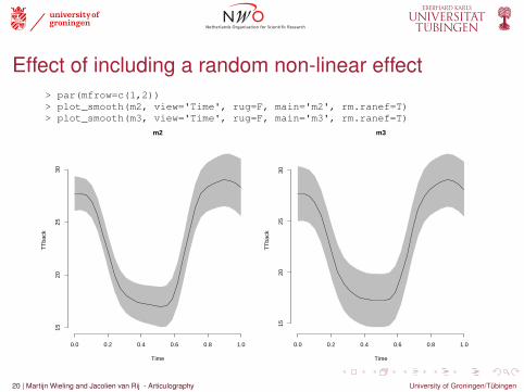
Effect of including a random non-linear effect> par(mfrow=c(1,2))> plot_smooth(m2, view='Time', rug=F, main='m2', rm.ranef=T)> plot_smooth(m3, view='Time', rug=F, main='m3', rm.ranef=T)

0.0 0.2 0.4 0.6 0.8 1.0

1520

2530

m2

Time

TT

back

0.0 0.2 0.4 0.6 0.8 1.0

1520

2530

m3

Time

TT

back


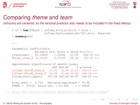
Comparing theme and team(smooths are centered, so the factorial predictor also needs to be included in the fixed effects)

> m4 = bam(TTback ~ s(Time,k=15,by=Word) + Word +s(Time,Participant,bs='fs',m=1), data=tm)

> summary(m4)

...


(Intercept) 25.16649 1.16592 21.59 <2e-16 ***Word@_theme_@ -4.18243 0.07096 -58.94 <2e-16 ***


s(Time):Word@_team_@ 11.81 13.04 19.27 <2e-16 ***s(Time):Word@_theme_@ 12.48 13.46 45.02 <2e-16 ***s(Time,Participant) 327.48 368.00 89.87 <2e-16 ***


I Does the correct-incorrect distinction improve the model?


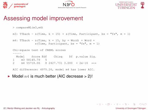
Assessing model improvement> compareML(m3,m4)

m3: TTback ~ s(Time, k = 15) + s(Time, Participant, bs = "fs", m = 1)

m4: TTback ~ s(Time, k = 15, by = Word) + Word +s(Time, Participant, bs = "fs", m = 1)

Chi-square test of fREML scores-----Model Score Edf Chisq Df p.value Sig.

1 m3 58145.79 52 m4 55718.06 8 2427.731 3.000 < 2e-16 ***

AIC difference: 4975.26, model m4 has lower AIC.

I Model m4 is much better (AIC decrease > 2)!


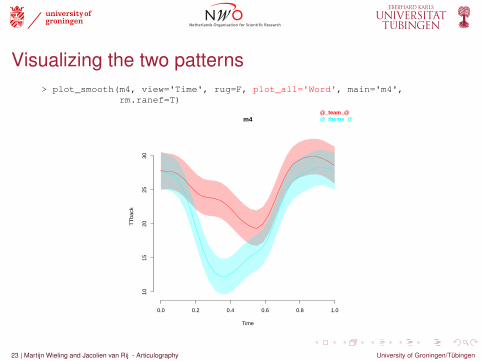
Visualizing the two patterns> plot_smooth(m4, view='Time', rug=F, plot_all='Word', main='m4',

rm.ranef=T)

0.0 0.2 0.4 0.6 0.8 1.0

1015

2025

30

m4

Time

TT

back

@_team_@@_theme_@


Visualizing the difference(no individual variation w.r.t. the difference is taken into account: confidence bands too thin)

> plot_diff(m4, view='Time', comp=list(Word=c('@_theme_@','@_team_@')),ylim=c(-12,2), rm.ranef=T)

0.0 0.2 0.4 0.6 0.8 1.0

−12

−10

−8

−6

−4

−2

02

Difference between @_theme_@ and @_team_@

Time

Est

. diff

eren

ce in

TT

back


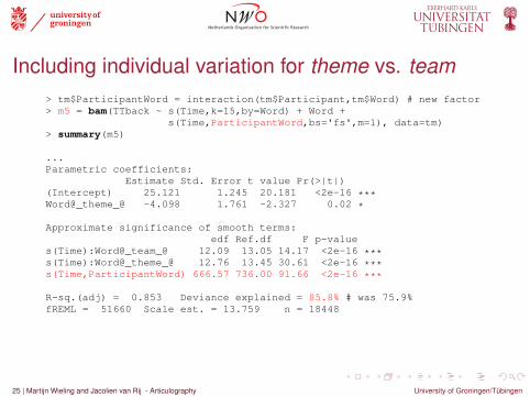
Including individual variation for theme vs. team> tm$ParticipantWord = interaction(tm$Participant,tm$Word) # new factor> m5 = bam(TTback ~ s(Time,k=15,by=Word) + Word +

s(Time,ParticipantWord,bs='fs',m=1), data=tm)> summary(m5)


Estimate Std. Error t value Pr(>|t|)(Intercept) 25.121 1.245 20.181 <2e-16 ***Word@_theme_@ -4.098 1.761 -2.327 0.02 *


s(Time):Word@_team_@ 12.09 13.05 14.17 <2e-16 ***s(Time):Word@_theme_@ 12.76 13.45 30.61 <2e-16 ***s(Time,ParticipantWord) 666.57 736.00 91.66 <2e-16 ***

R-sq.(adj) = 0.853 Deviance explained = 85.8% # was 75.9%fREML = 51660 Scale est. = 13.759 n = 18448


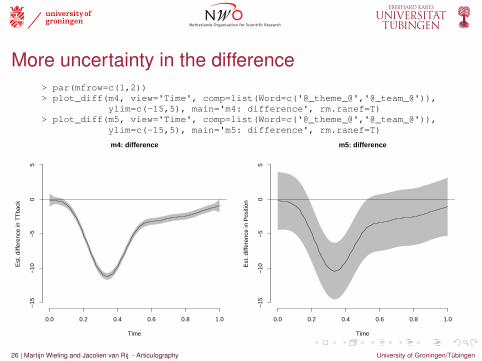
More uncertainty in the difference> par(mfrow=c(1,2))> plot_diff(m4, view='Time', comp=list(Word=c('@_theme_@','@_team_@')),

ylim=c(-15,5), main='m4: difference', rm.ranef=T)> plot_diff(m5, view='Time', comp=list(Word=c('@_theme_@','@_team_@')),

ylim=c(-15,5), main='m5: difference', rm.ranef=T)

0.0 0.2 0.4 0.6 0.8 1.0

−15

−10

−5

05

m4: difference

Time

Est

. diff

eren

ce in

TT

back

0.0 0.2 0.4 0.6 0.8 1.0

−15

−10

−5

05

m5: difference

Time

Est

. diff

eren

ce in

Pos

ition


Autocorrelation in the data is a problem!(residuals should be independent, otherwise the standard errors and p-values are wrong)

# It is essential that the data is sorted per individual trajectory> tm = start_event(tm, event=c("Participant","Word","RecBlock"))

> m5acf = acf_resid(m5) # show autocorrelation> rhoval = m5acf[2]> rhoval[1] 0.9527261 # correlation of residuals at time t with those at time t-1

0 10 20 30 40

0.0

0.2

0.4

0.6

0.8

1.0

ACF of resid_gam(model)

AC

F fu

nctio

n (p

er ti

me

serie

s)


Correcting for autocorrelation> m6 = bam(TTback ~ s(Time,k=15,by=Word) + Word +

s(Time,ParticipantWord,bs='fs',m=1), data=tm,rho=rhoval, AR.start=start.event)

> summary(m6)


Estimate Std. Error t value Pr(>|t|)(Intercept) 25.193 1.167 21.595 <2e-16 ***Word@_theme_@ -4.068 1.650 -2.465 0.0137 *


s(Time):Word@_team_@ 12.41 13.32 14.86 <2e-16 ***s(Time):Word@_theme_@ 12.95 13.59 32.27 <2e-16 ***s(Time,ParticipantWord) 555.16 736.00 5.51 <2e-16 ***



Autocorrelation has been removed> par(mfrow=c(1,2))> acf_resid(m5, main='ACF of m5')> acf_resid(m6, main='ACF of m6')

0 10 20 30 40

0.0

0.2

0.4

0.6

0.8

1.0

ACF of m5

AC

F fu

nctio

n (p

er ti

me

serie

s)

0 10 20 30 40

−0.

20.

00.

20.

40.

60.

81.

0

ACF of m6

AC

F fu

nctio

n (p

er ti

me

serie

s)


Clear model improvement> compareML(m5,m6)

m5: Position ~ s(Time, k = 15, by = Word) + Word +s(Time, ParticipantWord, bs = "fs", m = 1)

m6: Position ~ s(Time, k = 15, by = Word) + Word +s(Time, ParticipantWord, bs = "fs", m = 1)

Model m6 preferred: lower fREML score (24950.265), and equal df (0.000).-----Model Score Edf Difference Df

m5 51660.09 81 m6 26709.83 8 -24950.265 0.000

Warning message:In compareML(m5, m6) :

AIC is not reliable, because an AR1 model is included(rho1 = 0.000000, rho2 = 0.952726).


Distinguishing the two speaker groups> tm$WordGroup = interaction(tm$Word,tm$Group)> m7 = bam(TTback ~ s(Time,k=15,by=WordGroup) + WordGroup +

s(Time,ParticipantWord,bs='fs',m=1), data=tm,rho=rhoval, AR.start=start.event)

> summary(m7)


Estimate Std. Error t value Pr(>|t|)(Intercept) 27.497 1.452 18.938 < 2e-16 ***WordGroup@[email protected] -4.944 2.055 -2.406 0.016135 *WordGroup@[email protected] -4.896 2.132 -2.297 0.021640 *WordGroup@[email protected] -7.987 2.134 -3.742 0.000183 ***


s(Time):WordGroup@[email protected] 12.308 13.28 12.884 < 2e-16 ***s(Time):WordGroup@[email protected] 12.781 13.53 27.256 < 2e-16 ***s(Time):WordGroup@[email protected] 9.026 10.75 4.531 9.89e-07 ***s(Time):WordGroup@[email protected] 11.365 12.69 9.777 < 2e-16 ***s(Time,ParticipantWord) 535.302 734.00 4.789 < 2e-16 ***

R-sq.(adj) = 0.843 Deviance explained = 84.8%


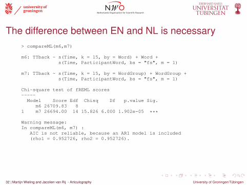
The difference between EN and NL is necessary> compareML(m6,m7)

m6: TTback ~ s(Time, k = 15, by = Word) + Word +s(Time, ParticipantWord, bs = "fs", m = 1)

m7: TTback ~ s(Time, k = 15, by = WordGroup) + WordGroup +s(Time, ParticipantWord, bs = "fs", m = 1)

Chi-square test of fREML scores-----Model Score Edf Chisq Df p.value Sig.

m6 26709.83 81 m7 26694.00 14 15.826 6.000 1.902e-05 ***

Warning message:In compareML(m6, m7) :

AIC is not reliable, because an AR1 model is included(rho1 = 0.952726, rho2 = 0.952726).


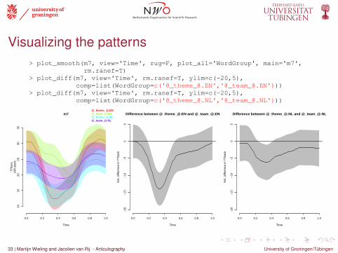
Visualizing the patterns> plot_smooth(m7, view='Time', rug=F, plot_all='WordGroup', main='m7',

rm.ranef=T)> plot_diff(m7, view='Time', rm.ranef=T, ylim=c(-20,5),

comp=list(WordGroup=c('@[email protected]','@[email protected]')))> plot_diff(m7, view='Time', rm.ranef=T, ylim=c(-20,5),

comp=list(WordGroup=c('@[email protected]','@[email protected]')))

0.0 0.2 0.4 0.6 0.8 1.0

1015

2025

3035

m7

Time

TT

back

(AR

.sta

rt)

@[email protected]@[email protected]@[email protected]@[email protected]

0.0 0.2 0.4 0.6 0.8 1.0

−20

−15

−10

−5

05

Difference between @[email protected] and @[email protected]

Time

Est

. diff

eren

ce in

TT

back

0.0 0.2 0.4 0.6 0.8 1.0

−20

−15

−10

−5

05

Difference between @[email protected] and @[email protected]

TimeE

st. d

iffer

ence

in T

Tba

ck


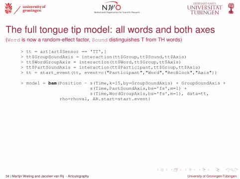
The full tongue tip model: all words and both axes(Word is now a random-effect factor, Sound distinguishes T from TH words)

> tt = art[art$Sensor == 'TT',]> tt$GroupSoundAxis = interaction(tt$Group,tt$Sound,tt$Axis)> tt$WordGroupAxis = interaction(tt$Word,tt$Group,tt$Axis)> tt$PartSoundAxis = interaction(tt$Participant,tt$Group,tt$Axis)> tt = start_event(tt, event=c("Participant","Word","RecBlock","Axis"))

> model = bam(Position ~ s(Time,k=15,by=GroupSoundAxis) + GroupSoundAxis +s(Time,PartSoundAxis,bs='fs',m=1) +s(Time,WordGroupAxis,bs='fs',m=1), data=tt,

rho=rhoval, AR.start=start.event)


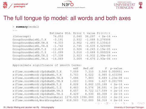
The full tongue tip model: all words and both axes> summary(model)...

Estimate Std. Error t value Pr(>|t|)(Intercept) 74.053 2.040 36.297 < 2e-16 ***GroupSoundAxisNL.T.X -3.191 2.932 -1.088 0.276508GroupSoundAxisEN.TH.X -4.333 2.902 -1.493 0.135410GroupSoundAxisNL.TH.X -1.742 2.745 -0.635 0.525590GroupSoundAxisEN.T.Z -12.419 2.926 -4.245 2.19e-05 ***GroupSoundAxisNL.T.Z -11.099 3.010 -3.688 0.000226 ***GroupSoundAxisEN.TH.Z -17.338 2.923 -5.932 2.99e-09 ***GroupSoundAxisNL.TH.Z -14.069 3.009 -4.676 2.93e-06 ***


s(Time.normWord):GpSdAxEN.T.X 7.059 7.310 3.566 0.000651 ***s(Time.normWord):GpSdAxNL.T.X 5.703 6.022 0.985 0.433398s(Time.normWord):GpSdAxEN.TH.X 7.686 7.883 6.689 1.23e-08 ***s(Time.normWord):GpSdAxNL.TH.X 1.003 1.006 1.627 0.201799s(Time.normWord):GpSdAxEN.T.Z 8.828 8.862 135.188 < 2e-16 ***s(Time.normWord):GpSdAxNL.T.Z 8.483 8.576 38.591 < 2e-16 ***s(Time.normWord):GpSdAxEN.TH.Z 8.657 8.722 117.599 < 2e-16 ***s(Time.normWord):GpSdAxNL.TH.Z 8.429 8.530 40.308 < 2e-16 ***s(Time.normWord,PartSoundAxis) 1276.029 1396.000 22.022 < 2e-16 ***s(Time.normWord,WordGroupAxis) 618.503 712.000 58.318 < 2e-16 ***


A clear L1-based pattern> par(mfrow=c(1,2))> plot_diff(m8, view='Time', rm.ranef=T, ylim=c(-20,10),

comp=list(GroupSoundAxis=c('EN.TH.X','EN.T.X')))> plot_diff(m8, view='Time', rm.ranef=T, ylim=c(-20,10),

comp=list(GroupSoundAxis=c('NL.TH.X','NL.T.X'))

0.0 0.2 0.4 0.6 0.8 1.0

−20

−15

−10

−5

05

10

Difference between EN.TH.X and EN.T.X

Time

Est

. diff

eren

ce in

Pos

ition

0.0 0.2 0.4 0.6 0.8 1.0

−20

−15

−10

−5

05

10

Difference between NL.TH.X and NL.T.X

Time

Est

. diff

eren

ce in

Pos

ition


2D visualization> source('plotArt2D.R')> plotArt2D(m, catvar="GroupSoundAxis", catlevels.x=c("NL.T.X","NL.TH.X"),

catlevels.y=c("NL.T.Z","NL.TH.Z"),collabels=c("NL: T","NL: TH"))# repeated for models for TM and TB (with parameter add=T)


DiscussionI Native English speakers appear to make the /t/-/T/ distinction, whereas

Dutch L2 speakers of English generally do notI Obviously, the model could be improved by separating minimal pairs into

two categories (which?)


RecapI We have applied GAMs to articulography data and learned how to:

I use s(Time) to model a non-linearity over timeI use the k parameter to control the ‘wigglyness’ of the non-linearityI use the plotting functions plot_smooth and plot_diffI use the parameter setting bs="re" to add random intercepts and slopesI add non-linear random effects using s(Time,...,bs="fs",m=1)I use the by-parameter to obtain separate non-linearities

I note that the factorial predictor used for the by-part needs to be included asfixed-effect factor as well!

I use compareML to compare models


Thank you for your attention!


Example of applying GAM: Articulographyjvanrij/LSA2015/sheets.pdf · Example of applying GAM:...

Documents

Transcript of Example of applying GAM: Articulographyjvanrij/LSA2015/sheets.pdf · Example of applying GAM:...