Physica B 423 (2013) 31–37

Contents lists available at SciVerse ScienceDirect

Physica B

0921-45http://d

n CorrE-m

journal homepage: www.elsevier.com/locate/physb

Exact numerical solutions of the Schrödinger equation fora two-dimensional exciton in a constant magnetic field ofarbitrary strength

Ngoc-Tram Hoang-Do a, Dang-Lan Phamb, Van-Hoang Le a,n

a Department of Physics, Ho Chi Minh City University of Pedagogy 280, An Duong Vuong Street, District 5, Ho Chi Minh City, Vietnamb Institute for Computational Science and Technology, Quang Trung Software Town, District 12, Ho Chi Minh City, Vietnam

a r t i c l e i n f o

Article history:Received 22 March 2013Received in revised form10 April 2013Accepted 11 April 2013Available online 30 April 2013

Keywords:Two-dimensional excitonExact solutionSchrödinger equationMagnetic field

26/$ - see front matter & 2013 Elsevier B.V. Ax.doi.org/10.1016/j.physb.2013.04.040

esponding author. Tel.: +84 8 38352020-109;ail address: hoanglv@hcmup.edu.vn (V.-H. Le)

a b s t r a c t

Exact numerical solutions of the Schrödinger equation for a two-dimensional exciton in a constantmagnetic field of arbitrary strength are obtained for not only the ground state but also high excitedstates. Toward this goal, the operator method is developed by combining with the Levi-Civitatransformation which transforms the problem under investigation into that of a two-dimensionalanharmonic oscillator. This development of the non-perturbation method is significant because it can beapplied to other problems of two-dimensional atomic systems. The obtained energies and wavefunctions set a new record for their precision of up to 20 decimal places. Analyzing the obtained datawe also find an interesting result that exact analytical solutions exist at some values of magnetic fieldintensity.

& 2013 Elsevier B.V. All rights reserved.

1. Introduction

A two-dimensional exciton in a magnetic field has been of greatinterest to both theoretical and experimental researchers for manyyears [1–5] and continues to be after several new and interestingphysical effects were discovered in recent years [6–10]. The energyspectrum and wavefunction of an exciton in magnetic field,therefore, need to be calculated with increasing precision. Sincethe 1990s, the perturbation method, the variational method andsome other numerical methods have been employed to calculatethe energy of this system in weak and strong magnetic field [2–4].The solution of the problem for a medium magnetic field wascalculated using extrapolation (see [3] and references therein).Note that there are some powerful methods which were devel-oped for finding the numerical solutions of the problems withinteraction potentials of general shape, see for example Refs.[11,12] for the potential morphing method.

In the last decade, however, solving the problem with higherprecision was preferred. In the work [13], the problem was solvedusing the mixed-basis variational method in combination with theshifted 1=N method, while in the work [14], the asymptoticiteration method was employed. Both of these methods providedsolutions with a precision of up to seven decimal places for theground state 1s and the excited states 2p− and 3d− only. Numericalresults for higher excited states have not been obtained up till

ll rights reserved.

fax: +84 8 38398946..

now. As per our understanding, increasing the precision andapplying these methods to higher excited states are not easy andare inefficient in terms of computing resources. Therefore, in ourpoint of view, developing a new method to calculate energy andwavefunctions for not only the ground state but also other highexcited states with any given precision is of interest.

In this work, we will use the operator method originated inRefs. [15,16] to obtain exact numerical solutions of the Schrödingerequation for a two-dimensional exciton in a constant magneticfield of arbitrary strength. The operator method was constructedby Komarov and Feranchuk in the 1980s and was employed tosolve the Schrödinger equation for several different physicalsystems (for an overview, see [17] and references therein; see also[18,19] for more recent works). To distinguish this method frommany other operator methods, in this paper we will refer to it asthe FK operator method. This method is similar to the perturbationtheory method in the splitting of the Hamiltonian into twocomponents: (i) the major component whose exact analyticalsolutions can be derived and (ii) the perturbation componentwhich is taken into account through corrections to energies andwavefunctions. However, the splitting of the Hamiltonian in theoperator method simply bases on the representation ofthe creation and annihilation operators. In addition, by changingthe value of a free parameter we can regularize the comparisonbetween the major component and the perturbation. That makesthe FK operator method applicable to non-perturbation problems.Furthermore, schemes of calculating high-order terms of correc-tions allow finding exact numerical solutions with a given preci-sion with a high convergence rate [20–23].

N.-T. Hoang-Do et al. / Physica B 423 (2013) 31–3732

Unfortunately, the FK operator method can not be applieddirectly to atomic systems because the expression of Coulombinteraction which contains coordinates in the denominator can notbe calculated using algebraic transformations of the creation andannihilation operators. We will overcome this difficulty of the FKoperator method by using the Levi-Civita transformation [24].According to the work [25], a two-dimensional exciton problemthrough the Levi-Civita transformation is equivalent to a harmonicoscillator problem. This connection makes it possible to obtain thewavefunctions of a two-dimensional exciton in an algebraic formwhich is very convenient for calculation. This leads us to using theLevi-Civita transformation to transform the problem of a two-dimensional exciton in magnetic field into that of an anharmonicoscillator in order to apply the FK operator method. The obtainedresults are interesting in the meaning of developing a non-perturbation method for two-dimensional atomic systems, whichcan be applied to other specific problems of interest in recentyears, such as those mentioned in Refs. [26,27].

In this work, new results are obtained while applying thedeveloped FK operator method to the problem of a two-dimensional exciton in a magnetic field. In principle, we canobtain both energies and wave functions with any given precision(exact numerical solutions) for any given state. Particularly, wedevelop an algorithm to get solutions with precision of up to 20decimal places due to the high convergence rate of this method.For the ground state 1s and the low excited states 2p− and 3d−,whose results were presented with a precision of seven decimalplaces in Refs. [13,14], our results include these seven decimalplaces. Moreover, the computing program can be used to calculateenergies and wavefunctions for any high excited states with theprincipal quantum number of up to 150. This is a new record.While analyzing the obtained data, we also find an interestingresult: the values of magnetic field intensity at which the exactanalytical solutions of the problem exist.

The structure of this paper is as follows. After this introductioncomes the section on theoretical and computational methods. Wefirst introduce the Schrödinger equation of the system through theLevi-Civita transformation. Then we present the basic steps andthe general principles of the FK operator method and derive thenecessary formula for applying the FK operator method to theproblem. In Section 3, we present the numerical results for theground state as well as high excited states. Some discussions aregiven in this section too. Finally, the conclusion section sum-marizes the new results of this work and proposes some ideas forfollow-up research.

2. Theoretical and computational methods

2.1. The Schrödinger equation through the Levi-Civitatransformation

In this section, the Levi-Civita transformation [24] is used totransform the Schrödinger equation of a two-dimensional excitonin a magnetic field into that of a two-dimensional anharmonicoscillator. The idea for this relation comes from our previous work[25] and the relation is originated in this paper.

For a two-dimensional exciton in a magnetic field we considerthe following Schrödinger equation written in atomic unit:

HΨ ðrÞ ¼ EΨ ðrÞ; ð1Þ

H ¼ −12

∂2

∂x2þ ∂2

∂y2

� �−iγ2

x∂∂y

−y∂∂x

� �þ 1

8γ2ðx2 þ y2Þ− Z

r: ð2Þ

Here, the effective Rydberg constant: Rn ¼mne4=16π2ε20ℏ2 is an

energy unit; the coordinates are measured in units of the effective

Bohr radius: an ¼ 4πε0ℏ2=mne2 and the dimensionless parameter γis defined by the formula γ ¼ ℏωc=2Rn with the cyclotron frequencyωc ¼ eB=2πmn and the magnetic field intensity B; mn, ε are theelectron effective mass and the static dielectric constant, respec-tively; Z is the charge of the hole, which equals 1 in this case tocompare the obtained results with those in Refs. [13,14]. In thiswork, we consider a wide range of γ covering both weak andstrong magnetic field regions.

We will now consider the Eqs. (1) and (2) in another spacewhich is more convenient for calculation through the Levi-Civitatransformation [21]:

x¼ u2−v2

y¼ 2uv:

(ð3Þ

The transformation (3) connects the two real two-dimensionalspaces ðx; yÞ and (u,v). We can easily prove the following equal-ities:

dx dy¼ 4ðu2 þ v2Þ du dv;

r¼ffiffiffiffiffiffiffiffiffiffiffiffiffiffiffiffix2 þ y2

q¼ u2 þ v2 ð4Þ

which will be used in the following calculation.From Eq. (4) we see that the Jacobian of the transformation (3)

is not a constant but is instead 4ðu2 þ v2Þ, so it will appear as aweight in the equation for calculating the scalar product of twostate vectors when transforming from the ðx; yÞ space to the ðu; vÞspace. This means that if a certain operator K is hermitian in theðx; yÞ space then the operator ~K ¼ 4ðu2 þ v2ÞK is also hermitian inthe ðu; vÞ space. Hence, in order to ensure that the Hamiltonian ishermitian through the transformation (3), we need to rewriteEq. (1) as follows:

rðH−EÞΨ ðrÞ ¼ 0:

In the ðu; vÞ space, this equation reads

~HΨ ðu; vÞ ¼ ZΨ ðu; vÞ ð5Þwith the Hamiltonian:

~H ¼−18

∂2

∂u2 þ∂2

∂v2

� �− E−

γ

2Lz

� �ðu2 þ v2Þ þ γ2

8ðu2 þ v2Þ3: ð6Þ

We see in Eqs. (5) and (6) an interchange of Z and E in the roleof the eigenvalue. The energy E is no longer the eigenvalue but isinstead a parameter, while Z becomes the eigenvalue of Eq. (5).However, we can still solve the Schrödinger equation to find Ewhen keeping Z¼1 as presented in the following section. Further-more, in the Hamiltonian (6) there is also the operator Lz which isthe orbital angular momentum operator. Because the systemunder investigation is two-dimensional, this operator is also itsprojection operator on a direction perpendicular to the plane ofmotion. In the ðu; vÞ space, this operator reads

Lz ¼−i2

u∂∂v

−v∂∂u

� �: ð7Þ

We can also prove that Lz commutes with the Hamiltonian of Eq.(5). This means that angular momentum is conserved in theproblem under consideration. We will use this conservation byconstructing a basis set for solving Eq. (5) which contains theeigenfunctions of the orbital angular momentum operator. Thenwe replace Lz by its eigenvalue in the Hamiltonian (5). Now wecan see that the Eqs. (5) and (6) represent a two-dimensionalanharmonic oscillator. In other words, we have transformed a two-dimensional exciton in magnetic field into an anharmonic oscilla-tor via the Levi-Civita transformation. This result allows theapplication of the FK operator method to find the exact numericalsolutions of Eqs. (5) and (6).

N.-T. Hoang-Do et al. / Physica B 423 (2013) 31–37 33

2.2. The FK operator method for solving the Schrödinger equation

The FK operator method is introduced in details in the work[15,16]. Here, we will only present the basic steps via solving theSchrödinger equations (5) and (6). The method includes four steps,as follows.

Step 1 is writing the Hamiltonian in algebraic form

~H∂∂u

;∂∂v

;u; v; γ� �

- ~Hða; b; aþ; b

þ; γÞ ð8Þ

using the creation and annihilation operators defined as follows:

aðωÞ ¼ffiffiffiffiω

2

rξþ 1

ω

∂∂ξn

� �; aþðωÞ ¼

ffiffiffiffiω

2

rξn−

1ω

∂∂ξ

� �;

bðωÞ ¼ffiffiffiffiω

2

rξn þ 1

ω

∂∂ξ

� �; b

þðωÞ ¼ffiffiffiffiω

2

rξ−

1ω

∂∂ξn

� �; ð9Þ

in which the complex coordinates are defined as ξ¼ uþ iv,ξn ¼ u−iv. We can easily check that the operators (9) satisfy thewell-known commutation relations:

½a; aþ� ¼ 1; ½b; bþ� ¼ 1: ð10ÞIn definition (9), we use complex coordinates for convenience inwriting only. The positive real number ω given in Eq. (9) isconsidered a free parameter whose role in the method will bediscussed in the next steps.

Plugging (9) into (6) we obtain the algebraic form of theHamiltonian as follows:

~Hðaþ; b

þ; a; b; γÞ ¼ ω2−2E þmγ

4ωðaþa þ b

þb þ 1Þ

−ω2 þ 2E−mγ

4ωðaþb

þ þ abÞ

þ γ2

64ω3 ðaþb

þ þ ab þ aþa þ bþb þ 1Þ3: ð11Þ

We also have an algebraic form of the orbital angular momentumoperator:

Lz ¼ −12ða

þa−bþbÞ; ð12Þ

which is a neutral operator.Step 2 is splitting the Hamiltonian (12) into two components–

the major component and the perturbation one:

~Hðaþ; b

þ; a; b; γÞ ¼ ~H0ðaþa; b

þb; γ;ωÞ þ ~V ðaþ

; bþ; a; b; γ;ωÞ: ð13Þ

The separation (13) is done based on a completely differentprinciple from that of the perturbation method. Here, the majorcomponent contains only neutral operators which are products ofequal number of creation and annihilation operators:

~H0ðaþa; bþb; γ;ωÞ ¼ ω2−2E þmγ

4ωðaþa þ b

þb þ 1Þ

þ γ2

64ω3 ðaþa þ b

þb þ 1Þ½ðaþa þ b

þb þ 1Þ

ðaþa þ bþb þ 4Þ

þ 6aþabþb þ 2�: ð14Þ

The rest is the perturbation term:

~V ðaþ; b

þ; a; b; γ;ωÞ

¼−ω2 þ 2E−mγ

4ωðaþb

þ þ abÞ þ γ2

64ω3 ½ðaþb

þÞ3 þ ðabÞ3

þ3aþbþðaþa þ b

þb þ 1Þ2 þ 3ðaþb

þÞ2ðaþa þ bþb þ 1Þ

þ3ðaþa þ bþb þ 1ÞðabÞ2 þ 3ðaþb

þÞ2ðabÞ þ 3aþbþðabÞ2

þ3ðaþa þ bþb þ 1Þ2ab þ 9aþb

þðaþa þ bþb þ 1Þ

þ9ðaþa þ bþb þ 1Þab þ 6ðaþb

þÞ2 þ 6ðabÞ2 þ 6aþbþ þ 6ab�:

ð15Þ

We see that the operator ~H0ðaþa; bþb; γ;ωÞ commutes with the

operators aþa and bþb, hence its exact solutions are the wave-

functions of the harmonic oscillator described by these operators.Furthermore, notice that although the Hamiltonian of the systemdoes not depend on the free parameter ω, the split components~H0ðaþa; b

þb; γ;ωÞ and ~V ðaþ

; bþ; a; b; γ;ωÞ do. This means that we

can adjust the correlation between the major and the perturbationcomponents by changing the value of ω.

Step 3 is finding the zeroth-order energy and wavefunctionusing the approximate Hamiltonian ~H0ðaþa; b

þb; γ;ωÞ. This

Hamiltonian contains only neutral operators aþa and bþb, so its

eigenfunctions have the following form:

ðaþÞjðbþÞkj0ðωÞ⟩ ð16Þin which j, k are non-negative integers and the vacuum state j0ðωÞ⟩is defined from the equations:

aðωÞj0ðωÞ⟩¼ 0; bðωÞj0ðωÞ⟩¼ 0; ð17Þand the normalization equation:

⟨0ðωÞj0ðωÞ⟩¼ 1: ð18ÞAs said in Section 2.1, angular momentum is conserved in the

problem under consideration. We will use this conservation byconstructing a basis set which contains the eigenfunctions of theorbital angular momentum operator Lz . This operator in thealgebraic form (12) is also a neutral operator, hence its eigenfunc-tions are also in the form (16). Therefore, the wavefunction vectors(16) are rewritten in normalization form as follows:

jnðmÞ⟩¼ 1ffiffiffiffiffiffiffiffiffiffiffiffiffiffiffiffiffiffiffiffiffiffiffiffiffiffiffiffiffiffiffiffiðn−mÞ!ðnþmÞ!

p ðaþÞn−mðbþÞnþmj0ðωÞ⟩ ð19Þ

in which the principal quantum numbers n are non-negativeintegers: n¼0, 1, 2,…, and the magnetic quantum numbers mare integers satisfying the condition −n≤m≤n. Furthermore, weuse the notation n¼ nr þ jmj in which nr ¼ 0, 1, 2, … are radialquantum numbers.

Thus we have the zeroth-order wavefunction corresponding tothe state of principal quantum number n and the magneticquantum numbers m:

jψnðmÞ⟩ð0Þ ¼ jnðmÞ⟩; ð20Þ

Now we let the Hamiltonian (14) act on the wavefunction (20) andconsider the Eq. (5). As a result, we obtain the zeroth-orderenergy:

Eð0Þ ¼ −2ωZ

2nþ 1þ 1

2ω2 þ γ2

16ω2 ð5n2 þ 5n−3m2 þ 3Þ þ 12mγ: ð21Þ

Here the free parameter is determined from the condition∂Eð0Þ=∂ω¼ 0 [15], which leads to the following equation:

−2Z

2nþ 1þ ω−

γ2

8ω3 ð5n2 þ 5n−3m2 þ 3Þ ¼ 0: ð22Þ

A numerical analysis of the analytical solutions (21) will begiven in the next section on results.

Step 4 is calculating high-order corrections to obtain exactnumerical solutions. In principle, we may use different schemes, e.g. the perturbation theory scheme for calculating high-ordercorrections in order to obtain the energy and the wavefunctionwith higher precision. If that scheme leads to a result thatconverges to a certain value with any given precision then wehave the exact numerical solution. In this work, we will propose aniteration scheme to calculate the energy and wavefunction with agiven precision.

For convenience we rewrite the Eqs. (5) and (6) as follows:

ð ~HR−E ~RÞjψ⟩¼ 0 ð23Þ

N.-T. Hoang-Do et al. / Physica B 423 (2013) 31–3734

in which the operator ~HRand ~R takes the following forms:

~HR ¼ ω2 þmγ

4ωðaþa þ b

þb þ 1Þ−ω2−mγ

4ωðaþb

þ þ abÞ

þ γ2

64ω3 ðaþb

þ þ ab þ aþa þ bþb þ 1Þ3−1;

~R ¼ 12ω

ðaþbþ þ ab þ aþa þ b

þb þ 1Þ: ð24Þ

We will use the basic set of wavefunctions (19) to construct thewavefunctions of the problem at hands. The matrix elements ofthe operators (24) corresponding to this basic set will be calcu-lated through purely algebraic transformation. In fact, using thecommutations (10) and the Eqs. (17) and (18), we easily obtainfollowing formula:

aþbþjnðmÞ⟩¼

ffiffiffiffiffiffiffiffiffiffiffiffiffiffiffiffiffiffiffiffiffiffiffiffiffiffiffiðnþ 1Þ2−m2

qjnþ 1ðmÞ⟩;

abjnðmÞ⟩¼ffiffiffiffiffiffiffiffiffiffiffiffiffiffiffin2−m2

pjn−1ðmÞ⟩;

ðaþa þ bþbÞjnðmÞ⟩¼ 2njnðmÞ⟩ ð25Þ

from which we calculate the matrix elements as follows:

HRnn ¼ ⟨nðmÞj ~HRjnðmÞ⟩

¼ ω2−mγ

4ωð2nþ 1Þ þ γ2

32ω3 ð2nþ 1Þð5n2 þ 5nþ 3−3m2Þ−Z;

HRn;nþ1 ¼ ⟨nðmÞj ~HRjnþ 1ðmÞ⟩¼

ffiffiffiffiffiffiffiffiffiffiffiffiffiffiffiffiffiffiffiffiffiffiffiffiffiffiffiðnþ 1Þ2−m2

q� −

ω2 þmγ

4ωþ 3γ2

64ω3 ð5n2 þ 10nþ 6−m2Þ� �

;

HRn;nþ2 ¼ ⟨nðmÞj ~HRjnþ 2ðmÞ⟩

¼ 3γ2

64ω3 ð2nþ 3Þffiffiffiffiffiffiffiffiffiffiffiffiffiffiffiffiffiffiffiffiffiffiffiffiffiffiffiðnþ 1Þ2−m2

q ffiffiffiffiffiffiffiffiffiffiffiffiffiffiffiffiffiffiffiffiffiffiffiffiffiffiffiðnþ 2Þ2−m2

q;

HRn;nþ3 ¼ ⟨nðmÞj ~HRjnþ 3ðmÞ⟩

¼ γ2

64ω3

ffiffiffiffiffiffiffiffiffiffiffiffiffiffiffiffiffiffiffiffiffiffiffiffiffiffiffiðnþ 1Þ2−m2

q ffiffiffiffiffiffiffiffiffiffiffiffiffiffiffiffiffiffiffiffiffiffiffiffiffiffiffiðnþ 2Þ2−m2

q ffiffiffiffiffiffiffiffiffiffiffiffiffiffiffiffiffiffiffiffiffiffiffiffiffiffiffiðnþ 3Þ2−m2

q;

Rnn ¼ ⟨nðmÞj ~RjnðmÞ⟩¼ 2nþ 12ω

;

Rn;nþ1 ¼ ⟨nðmÞj ~Rjnþ 1ðmÞ⟩¼−12ω

ffiffiffiffiffiffiffiffiffiffiffiffiffiffiffiffiffiffiffiffiffiffiffiffiffiffiffiðnþ 1Þ2−m2

q: ð26Þ

Besides (26), we can calculate other non-zero matrix elementsusing the symmetry properties HR

nk ¼HRkn, Rnk ¼ Rkn.

We can write the exact wavefunction as a linear combination ofthe basic functions (19):

jψnðmÞ⟩¼ jnðmÞ⟩þ ∑þ∞

j ¼ jmj;j≠nCjjjðmÞ⟩; ð27Þ

and define the approximate wavefunction at the s-th orderapproximation (s-th iteration loop) as

jψnðmÞ⟩ðsÞ ¼ jnðmÞ⟩þ ∑

nþs

j ¼ jmj;j≠nCðsÞj jjðmÞ⟩ ð28Þ

corresponding to the approximate energy EðsÞ. If lims-∞CðsÞk ¼ Ck

then the approximate wavefunction (28) converges to the exactwavefunction (27). If then we have EðsÞ-ET while s-þ ∞, we alsohave the exact energy. We will use the notations for quantumstates as in the work [13,14], e.g.: 1s, 2s, 2p−, 2pþ, 3s, 3p−, 3pþ, 3d−,3dþ, etc. The first digit stands for the state level nþ 1, in which n isthe principal quantum number defined in Eq. (19); the letterssymbolize the orbital quantum numbers l¼ jmj: s correspondingto l¼ 0, p to l¼1, d to l¼2, f to l¼3, g to l¼4, etc; the 7 sign is ofthe magnetic quantum number m.

Putting Eq. (28) into the Schrödinger equation (23), we obtainthe expression for the approximate s-th order energy:

EðsÞ ¼HR

nn þ∑nþsk ¼ jmj;k≠nC

ðsÞk HR

nk

Rnn þ∑nþsk ¼ jmj;k≠nC

ðsÞk Rnk

ð29Þ

in which the coefficients CðsÞk ðk¼ jmj; jmj þ 1;…;n−1;nþ 1;…;nþ

sÞ are determined by a system of nþ s−jmj linear equations:

∑nþs

k ¼ jmj;k≠n;k≠jðHR

jk−Eðs−1ÞÞCðsÞ

k ¼ RnjEðs−1Þ−HR

nj; ð30Þ

in which j¼ jmj; jmj þ 1;…;n−1;nþ 1;…;nþ s.So, by plugging the solutions of Eq. (30) into Eq. (29) we obtain

the energy of the system at the s-th iteration loop, which is calledthe s-th order approximation energy. Numerical results show thatwith appropriate choice of ω, for the considered problem weobtain a series of approximate energies

Eð0Þ; Eð1Þ; Eð2Þ;…; EðsÞ;… ð31Þ

which rapidly converges to a value ET. We call them the exactnumerical solutions because their values can be obtained with anygiven precision. In this work, we calculate these solutions withprecision of up to 20 decimal places due to the limitation of thedefault precision for real numbers in FORTRAN and the computingspeed of computer. However, this is an important progress. As weknow, the precision for real numbers in FORTRAN is limited to 15decimal places. By appropriate programming, we can increase thisprecision up to 50 decimal places. In our final results for energiesand wavefunctions, we require a precision of up to 20 decimalplaces in order to avoid the accumulation of errors in calculating.Besides energy, the coefficients CðsÞ

k also converge rapidly so weobtain not only exact numerical energy but also exact numericalwavefunctions.

The parameter ω is chosen using the method described in Refs.[20–23]. In principle, this parameter does not affect the exactnumerical results. However, investigation shows that the conver-gence rate to the exact solutions depends significantly on thechoice of ω. In this work, the equation ∂Eð0Þ=∂ω¼ 0 provides thefirst value ω0 which is not the optimal value. For high excitedstates nr, such a choice of ω even does not lead to convergence toexact values. We can scan to find the optimal value of parameteraround the first value of ω0. The results in this paper reconfirm theconclusions of Refs. [22,23] about the existence of the range ofparameter such that the convergence rate of Eq. (28) is highest.

3. Results and discussions

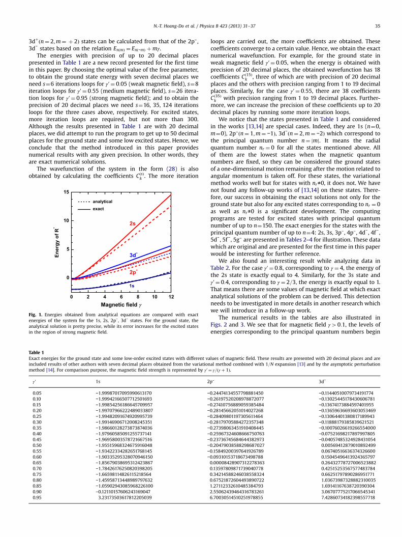
Analytical solutions: Fig. 1 shows the energies of the systemcorresponding to the ground state and some excited states 1s, 2s,2p−, 3d−. The dotted line represents the results, which can beconsidered analytical solutions, obtained with zeroth-orderapproximation using the Eqs. (20) and (21). The solid linerepresents the exact numerical results for comparison purposes.These exact results are obtained from the iteration Eqs. (26) and(27). On this figure, we see that the analytical solutions are prettyprecise for the ground and excited states in magnetic field regionγ ≤1. In stronger magnetic field, this precision decreases while thecorrelation between the energy levels stays the same. In order toobtain analytical solutions which are highly precise and areuniformly suitable in the whole range of magnetic field, we needto consider the asymptotic behavior of the wavefunction in strongmagnetic field region. We will discuss this case in another work.

Exact numerical solutions: In this work, we focus on exactnumerical solutions. Table 1 presents energies with precision ofup to 20 decimal places for the ground state 1s (n¼m¼0) andsome excited states 2p−ðn¼ 1;m¼ −1Þ, 3d−ðn¼ 2;m¼ −2Þ. Thesestates were calculated with the precision of up to seven decimalplaces in Refs. [13,14]. Here, the results in Refs. [13,14] are notshown because all of these seven places are included in our resultsshown in Table 1. The energy of the 2pþðn¼ 1;m¼ þ 1Þ,

N.-T. Hoang-Do et al. / Physica B 423 (2013) 31–37 35

3dþðn¼ 2;m¼ þ 2Þ states can be calculated from that of the 2p−,3d− states based on the relation EnðmÞ ¼ Enð−mÞ þmγ.

The energies with precision of up to 20 decimal placespresented in Table 1 are a new record presented for the first timein this paper. By choosing the optimal value of the free parameter,to obtain the ground state energy with seven decimal places weneed s¼6 iterations loops for γ′¼ 0:05 (weak magnetic field), s¼8iteration loops for γ′¼ 0:55 (medium magnetic field), s¼26 itera-tion loops for γ′¼ 0:95 (strong magnetic field); and to obtain theprecision of 20 decimal places we need s¼16, 35, 124 iterationsloops for the three cases above, respectively. For excited states,more iteration loops are required, but not more than 300.Although the results presented in Table 1 are with 20 decimalplaces, we did attempt to run the program to get up to 50 decimalplaces for the ground state and some low excited states. Hence, weconclude that the method introduced in this paper providesnumerical results with any given precision. In other words, theyare exact numerical solutions.

The wavefunction of the system in the form (28) is alsoobtained by calculating the coefficients CðsÞ

k . The more iteration

Fig. 1. Energies obtained from analytical equations are compared with exactenergies of the system for the 1s, 2s, 2p−, 3d− states. For the ground state, theanalytical solution is pretty precise, while its error increases for the excited statesin the region of strong magnetic field.

Table 1Exact energies for the ground state and some low-order excited states with different vaincluded results of other authors with seven decimal places obtained from the variationmethod [14]. For comparison purpose, the magnetic field strength is represented by γ′¼

γ′ 1s 2

0.05 −1.99987017095990613170 −0.10 −1.99942166507712501693 −0.15 −1.99854256186645709957 −0.20 −1.99707966222489033807 −0.25 −1.99482091674920995739 −0.30 −1.99146906712008245351 −0.35 −1.98660128273873874036 −0.40 −1.97960585091255737141 −0.45 −1.96958003578721667516 −0.50 −1.95515968324675916048 −0.55 −1.93422334282651768145 −0.60 −1.90335295328070946150 −0.65 −1.856790386953124238670.70 −1.784261762508203982050.75 −1.665981148261152185640.80 −1.459587134489897976320.85 −1.059029430859682261000.90 −0.121101576062431690470.95 3.23173503617812205039

loops are carried out, the more coefficients are obtained. Thesecoefficients converge to a certain value. Hence, we obtain the exactnumerical wavefunction. For example, for the ground state inweak magnetic field γ′¼ 0:05, when the energy is obtained withprecision of 20 decimal places, the obtained wavefunction has 18coefficients Cð15Þ

k , three of which are with precision of 20 decimalplaces and the others with precision ranging from 1 to 19 decimalplaces. Similarly, for the case γ′¼ 0:55, there are 38 coefficientsCð35Þk with precision ranging from 1 to 19 decimal places. Further-

more, we can increase the precision of these coefficients up to 20decimal places by running some more iteration loops.

We notice that the states presented in Table 1 and consideredin the works [13,14] are special cases. Indeed, they are 1s (n¼0,m¼0), 2p−ðn¼ 1;m¼ −1Þ, 3d−ðn¼ 2;m¼ −2Þ which correspond tothe principal quantum number n¼ jmj. It means the radialquantum number nr ¼ 0 for all the states mentioned above. Allof them are the lowest states when the magnetic quantumnumbers are fixed, so they can be considered the ground statesof a one-dimensional motion remaining after the motion related toangular momentum is taken off. For these states, the variationalmethod works well but for states with nr≠0, it does not. We havenot found any follow-up works of [13,14] on these states. There-fore, our success in obtaining the exact solutions not only for theground state but also for any excited states corresponding to nr ¼ 0as well as nr≠0 is a significant development. The computingprograms are tested for excited states with principal quantumnumber of up to n¼150. The exact energies for the states with theprincipal quantum number of up to n¼4: 2s, 3s, 3p−, 4p−, 4d−, 4f−,5d−, 5f−, 5g− are presented in Tables 2–4 for illustration. These datawhich are original and are presented for the first time in this paperwould be interesting for further reference.

We also found an interesting result while analyzing data inTable 2. For the case γ′¼ 0:8, corresponding to γ ¼ 4, the energy ofthe 2s state is exactly equal to 4. Similarly, for the 3s state andγ′¼ 0:4, corresponding to γ ¼ 2=3, the energy is exactly equal to 1.That means there are some values of magnetic field at which exactanalytical solutions of the problem can be derived. This detectionneeds to be investigated in more details in another research whichwe will introduce in a follow-up work.

The numerical results in the tables are also illustrated inFigs. 2 and 3. We see that for magnetic field γ40:1, the levels ofenergies corresponding to the principal quantum numbers begin

lues of magnetic field. These results are presented with 20 decimal places and areal method combined with 1=N expansion [13] and by the asymptotic perturbationγ=ðγ þ 1Þ.

p− 3d−

0.24474134557798881450 −0.114405100797341917740.26197520208978872077 −0.130254451784306067810.27410756889059385484 −0.136741738845974019550.28145662051014027268 −0.136596366936030534690.28409801197305611464 −0.130644013808171899430.28179705884272357348 −0.118881793858396215210.27398063451910408445 −0.100760266192665540000.25967324608666750763 −0.075216982178979978050.23736745684644382973 −0.040574853249284310540.20479038588298687027 0.005694128790108924990.15849200397641926789 0.067405166363743266000.09310153718673498788 0.150454964139243657970.00008428907312278363 0.264327787270065238820.13597809871739040778 0.425152535675774837840.34214588246038558324 0.662517978902869517710.67521872604493890722 1.036739873288823100351.27112332610485384793 1.691411676387203903042.55062439464316783261 3.067077752170665453416.70030514510251978855 7.42860734182398557718

Table 2Energies of some excited states corresponding to different values of the magnetic field.

γ′ 2s 3s 3p−

0.05 −0.21728279396968785397 −0.05137115812285705179 −0.080367217445031097600.10 −0.20160591618074023247 0.01598790970267759145 −0.049160514429008001500.15 −0.17457048111136615243 0.10955543404170749556 0.001086375654850448130.20 −0.13546551574551668372 0.22721834540118963879 0.067383285745485769580.25 −0.08298007150252920818 0.37047446264365413831 0.149867425553934446030.30 −0.01502952750059654076 0.54292733023387127727 0.250286330927010182440.35 0.07142846360607761967 0.75013268675298689141 0.371706685809471035020.40 0.18070180520537274524 1.000000000000000000 0.518674149921909535590.45 0.31887814627104300055 1.30366017149884873723 0.697693223741300950620.50 0.49467963883695179668 1.67697071075735877489 0.918103969140767381530.55 0.72091579831145684540 2.14309105414624009242 1.193603732087995518250.60 1.01705668872877975106 2.73703806534873385927 1.544951886135388146660.65 1.41405521488835508770 3.51419634203232951294 2.005032297898359648320.70 1.96407032991584636290 4.56741386886003820741 2.629032762735335364860.75 2.76203075990704173477 6.06476489650834377662 3.516945768406411846520.80 4.000000000000000000 8.34434942653877459541 4.870088643827444993700.85 6.13177508892586718321 12.19997778752228732308 7.161539172830629948290.90 10.53825335361872298997 20.02986405533713661963 11.821927929993232452340.95 24.24854780554921085193 43.93175572792464946928 26.07692664470341686614

Table 3Energies of some high excited states with n¼3 corresponding to different values of the magnetic field.

γ′ 4p− 4d− 4f−

0.05 0.00090050861670000681 −0.03603819112188519016 −0.077633150149928532550.10 0.09390796453557639448 0.00747840526168139693 −0.088035209105603539690.15 0.21323373403753960833 0.06842568965737196928 −0.088883396547016965100.20 0.35668048473475479870 0.14447370643180047832 −0.083153845878506371740.25 0.52606940637774516311 0.23628341974950389743 −0.071600764408019577700.30 0.72533207396702501971 0.34594127952399409512 −0.054122677560018326010.35 0.96036057230843709310 0.47676457059152532284 −0.030068281797265224150.40 1.23944041995229360305 0.63351735049084262159 0.001733999817239356160.45 1.57415466587235095938 0.82292516365874272605 0.043086724043883009100.50 1.98093584143111358970 1.05458031287213984997 0.096672132200198159810.55 2.48370977153057734079 1.34249561828604384524 0.166506436965593741340.60 3.11856112568506923453 1.70785470976146371028 0.258762681395305692810.65 3.94243430849379882861 2.18414967307751588723 0.383325868319778780520.70 5.05058514254628752285 2.82749853910929518464 0.556941419654148664510.75 6.61507130462100771829 3.73942662403763270927 0.810217014672505908970.80 8.98122289598444673098 5.12403034105099778843 1.205318439951101066720.85 12.95785147539592703023 7.46015607265407629634 1.889682019346875861460.90 20.98177530017893504943 12.19329771792373821144 3.313757037863218201170.95 45.30314463505568435467 26.60790678762850209795 7.78159090037994763851

Table 4Energies of some excited states with n¼4 corresponding to different values of the magnetic field.

γ′ 5d− 5f− 5g−

0.05 0.02905749316697708979 −0.01420058007237175099 −0.060078755194895160570.10 0.13341069872580500192 0.03570019722639813037 −0.066046579974867248540.15 0.26190026516127302629 0.10204170420617281261 −0.062922402313735308310.20 0.41356740099965750564 0.18308786847417280362 −0.053441450795155787040.25 0.59077510317782206889 0.27975368917130985634 −0.038211409306314375160.30 0.79776115680429092118 0.39427787158829185045 −0.017030675829675117600.35 1.04063336998574952266 0.53009357416698937372 0.010833727795669495260.40 1.32786142397127676506 0.69207101474623163562 0.046631241354599619390.45 1.67121288127923035467 0.88704788903212652389 0.092248544765636630440.50 2.08732965304714088906 1.12474823987081387279 0.150467905753425977240.55 2.60039856986566405608 1.41935251349090562787 0.225433626381684086450.60 3.24685460813888191684 1.79227191808221737000 0.323493223346459399860.65 4.08414376941622929138 2.27732643588718193308 0.454783502571012080930.70 5.20828847495739630265 2.93113687655407534814 0.636436312127864435370.75 6.79260902069767290808 3.85605806748978018262 0.899697145066917496330.80 9.18472403676149577875 5.25769124636313341999 1.307889091262950268710.85 13.19819451070249609938 7.61800718398620959057 2.010851566327854574930.90 21.28207427023502943214 12.39055080521797139007 3.465226537495143330960.95 45.73489523603524444325 26.89161351897346612252 7.99955272626774688799

N.-T. Hoang-Do et al. / Physica B 423 (2013) 31–3736

Fig. 2. The dependence of energy on magnetic field strength for the states withprincipal quantum number n¼3: 1s, 2s, 2p7 , 3s, 3p7 , 3d7 , 4p7 , 4d7 , 4f7 . Wesee that in strong magnetic fields, the degenerated Landau levels split out due toCoulomb interaction although they are still close to each other and are magnified in(a), (b), (c), and (d).

Fig. 3. Energy levels in γ ≤1 region of magnetic field.

N.-T. Hoang-Do et al. / Physica B 423 (2013) 31–37 37

to disarrange. For example, 2s and 2pþ levels are higher than 3d−

and 4f− levels; 3s and 3pþ are higher than 4d−, 4f− levels. That isbecause we use the principal quantum numbers of the Coulombproblemwhich is reasonable only in weak magnetic field. In strongmagnetic field, Coulomb interactions are considered a perturba-tion which eliminates the degenerate Landau levels. Thus, in thiscase the principal quantum numbers must follow Landau levels inthe problem of motion of electrons in a uniform magnetic field.Our finding of exact solutions for high excited states with principalquantum number of up to hundreds allows investigation of notonly the degenerate separation of Landau levels but also quantumchaos effects. These are some suggestions for further research.

4. Conclusion and outlook

In this work we obtain the following original results:

(1)

Transforming the problem of a two-dimensional exciton in amagnetic field into that of a two-dimensional anharmonicoscillator through Levi-Civita transformation. This is an impor-tant result because the problem of an anharmonic oscillator ismuch simpler and is well-investigated using several methods.

(2)

Successful development of the FK operator method for a two-dimensional exciton in a magnetic field. This development issignificant, universal and applicable to various problemsrelated to two-dimensional exciton in electromagnetic field.

(3)

Obtaining exact numerical solutions for a two-dimensionalexciton in a constant magnetic field with arbitrary strength.For the ground state and the excited states considered inprevious works of other authors, we set a new record onprecision of up to 20 decimal places. Furthermore, exactsolutions for high excited states are presented for the firsttime in this work. The FORTRAN program for calculatingenergies and wavefunctions of any excited states with princi-pal quantum number of up to hundreds can be provided tointerested researchers. These results can be used for researchrelated to the energy levels of a two-dimensional exciton in amagnetic field.

(4)

Detecting some concrete values of magnetic field strength atwhich the problem of a two-dimensional exciton in a magneticfield has exact analytical solutions. This detection is veryinteresting and needs more detailed research.

Acknowledgments

We would like to thank Professor Feranchuk I. D. (BelarusianState University, Minsk – Belarus) for careful reading and helpfulcomments on this work.

This work is sponsored by the National Foundation for Scienceand Technology Development (NAFOSTED) Grant no. 103.01-2011.08. The author Hoang-Do also would like to thank for theinstitutional grant provided by Ho Chi Minh City University ofPedagogy.

References

[1] D. Paquet, T.M. Rice, K. Ueda, Phys. Rev. B 32 (1985) 5208.[2] W. Edelstein, Phys. Rev. B 39 (1989) 7697.[3] Jia-Lin Zhu, Y. Cheng, Jia-Jiong Xiong, Phys. Rev. B 41 (1990) 10792.[4] A.B. Dzyubenko, Phys. Rev. B 64 (2001) 241101 (R).[5] L.V. Butov, C.W. Lai, D.S. Chemla, Yu.E. Lozovik, K.L. Campman, A.C. Gossard,

Phys. Rev. Lett. 87 (2001) 216804.[6] G.V. Astakhov, D.R. Yakolev, V.V. Rudenkov, P.C.H. Christianen, T. Barrick, S.

A. Gooker, A.B. Dzyubenko, W. Ossau, J.C. Maan, G. Karczewshi, T. Wojtowicz,Phys. Rev. B 71 (2005) 201312 (R).

[7] A. Bruno-Alfonso, L. Candido, G.Q. Hai, J. Phys.: Condens. Matter 22 (2010)125801.

[8] A. Poszwa, Phys. Scripta 84 (2011) 055002.[9] D. Nandi, A.D.K. Finck, J.P. Eisenstein, L.N. Pfeiffer, K.W. West, Nature 488

(2012) 481.[10] Z. Zeng, C.S. Garoufalis, S. Baskoutas, J. Phys. D 45 (2012) 235102.[11] Z. Zeng, E. Paspalakis, C.S. Garoufalis, Andreas F. Terzis, S. Baskoutas, J. Appl.

Phys. 113 (2013) 054303.[12] M. Rieth, W. Schommers, S. Baskoutas, Int. J. Mod. Phys. B 16 (2002) 4081.[13] V.M. Villalba, R. Pino, Physica B 315 (2002) 289.[14] A. Soylu, I. Boztosun, Physica E 40 (2008) 443.[15] I.D. Feranchuk, L.I. Komarov, Phys. Lett. A 88 (1982) 212.[16] I.D. Feranchuk, L.I. Komarov, I.V. Nichipor, A.P. Ulyanenkov, Ann. Phys. 238

(1995) 370.[17] I.D. Feranchuk, A. Ivanov, in: Etude on Theoretical Physics, World Scientific,

Singapore, 2004, pp. 171–188.[18] I.D. Feranchuk, A.V. Leonov, Phys. Lett. A 373 (2009) 517.[19] A.V. Leonov, I.D. Feranchuk, J. Appl. Spectrosc. 77 (2011) 832.[20] F.M. Fernandez, A.M. Meson, E.A. Castro, Phys. Lett. A 18 (1984) 401.[21] F.M. Fernandez, A.M. Meson, E.A. Castro, Phys. Lett. A 18 (1985) 104.[22] Chan Za An, I.D. Feranchuk, L.I. Komarov, L.S. Nakhamchik, J. Phys. A 19 (1986)

1583.[23] Quoc-Khanh Hoang, Van-Hoang Le, L.I. Komarov, Proceed. Acad. Sci. Belarus

(Phys. Math. Ser.) 3 (1997) 71.[24] T Levi-Civita, Opere Matematiche. Memorie e note. Vol. II. 1901-1907, (Nicola

Zanichelli Editore, Bologna, 1956).[25] Van-Hoang Le, Thu-Giang Nguyen, J. Phys. A 26 (1993) 1409.[26] J. Zhu, S.L. Ban, S.H. Ha, Phys. Status Solidi B 248 (2011) 384.[27] F. Milota, J. Sperling, A. Nemeth, T. Mancal, H.F. Kauffmann, Acc. Chem. Res. 42

(2009) 1364.