Exact differential for the thermodynamics

Masatsugu Sei Suzuki

Department of Physics, SUNY at Binghamton

Binghamton, NY 13902-6000

(date: September 05, 2018)

1. Exact differential

We work in two dimensions, with similar definitions holding in any other number of

dimensions. In two dimensions, a form of the type

dyyxBdxyxA ),(),(

is called a differential form. This form is called exact if there exists some scalar function ),( yxQ

BdyAdxdyy

Qdx

x

QdQ

xy

,

if and only if

yxx

B

y

A

or

yxxy y

Q

xx

Q

y

The vector field ),( BA is a conservative vector field, with corresponding potential Q. When a

differential Q is exact, the function Q exist,

)()( iQfQdQ

f

i

,

independent of the oath followed.

In thermodynamics, when dQ is exact, the function Q is a state function of the system. The

thermodynamics functions, E (or U) , S, H, F (or A), and G are state functions. An exact

differential is sometimes also called a total differential or a full differential.

2. Jacobian

We consider two functions u and v such that

),( yxuu , ),( yxvv

The Jacobian is defined as

y

v

x

v

y

u

x

u

yx

vu

),(

),(.

It clearly has the following properties

),(

),(

),(

),(

yx

vu

yx

uv

yx

uy

u

x

u

y

y

x

y

y

u

x

u

yx

yu

10),(

),(.

The following relations also hold:

),(

),(

1

),(

),(

vz

yxyx

yz

y

y

y

t

x

t

z

yt

yx

yt

yz

yx

yz

x

z

),(

),(

),(

),(

),(

),(

1),(

),(

),(

),(

),(

),(

xz

xy

zy

zx

yx

yz

ux

y

x

y

y

u

ux

uy

xy

xu

xu

yu

xy

xu

yx

yu

x

u

),(

),(

),(

),(

),(

),(

),(

),(

),(

),(

3. Expression of PC and VC

The heat capacity:

T

V

V

P

V

PT

VS

T

PT

VT

PT

VS

TVT

VST

T

STC

),(

),(

),(

),(

),(

),(

),(

),(

or

T

PT

P

PTTP

T

TP

TP

T

V

P

V

T

V

P

ST

T

ST

T

V

P

S

P

V

T

S

P

V

T

P

V

T

V

P

S

T

S

P

V

TC

][

Using the Maxwell’s relation

PT T

V

P

S

and the relation

T

T

V

P

TV

TPTP

TV

P

V

1

),(

),(

1

),(

),(

Then we get

TP

P

T

PPV

V

P

T

VTC

P

V

T

VT

CC

2

2

or

TP

VPV

P

T

VTCC

2

For the ideal gas we have the Mayer relation

RCC VP

This is one of the most important equations of thermodynamics, and it shows that:

(a) 0

TV

P, leading to VP CC

(b) As 0T , VP CC

(c) VP CC when 0

PT

V.

s

For example, at 4°C at which the density of water is maximum, VP CC .

Using the volume expansion and isothermal compressibility

PT

V

V

1

,

T

T

V

PVP

V

V

111

We may write the equation in the form

2TV

CC VP

4. Legendre transformation

Legendre transforms appear in two places in a standard undergraduate physics curriculum: (i)

in classical mechanics and (ii) in thermodynamics. The Legendre transform simply changes the

independent variables in a function of two variables by application of the product rule.

We start with the expression for the internal energy U as

PdVTdSdU

(a) Helmholtz free energy: F

Using the relation

PdVSdTTSddU )(

we have

PdVSdTTSUd )(

Here we introduce the Helmholtz free energy F as

STUF

Thus we have the relation

PdVSdTdF

(b) Enthalpy: H

From the relation

VdPPVdTdS

PdVTdSdU

)(

we have

VdPTdSPVUd )(

Here we introduce the enthalpy H as

PVUH

Thus we have

VdPTdSdH

(c) Gibbs Free energy:

Using the relation

VdPPVdSdT

PdVSdTdF

)(

we have

\

VdPSdTPVFd )(

We introduce the Gibbs free energy G as

PVFG

with

VdPSdTdG

5. Thermodynamic potential

Fig. Born diagram. UE (internal energy). FA (Helmholtz free energy).

(a) The internal energy ),( VSUU

For an infinitesimal reversible process, we have

PdVTdSdU

showing that

VS

UT

, SV

UP

and

VS S

P

V

T

(Maxwell’s equation)

(b) The enthalpy ),( PSHH

The enthalpy H is defined as

PVUH

S

V

T

P

E

FG

H

For an infinitesimal reversible process,

VdPPdVdUdH

but

PdVTdSdU

Therefore we have

VdPTdSdH

showing that

PS

HT

, SP

HV

and

PS S

V

P

T

. (Maxwell’s equation)

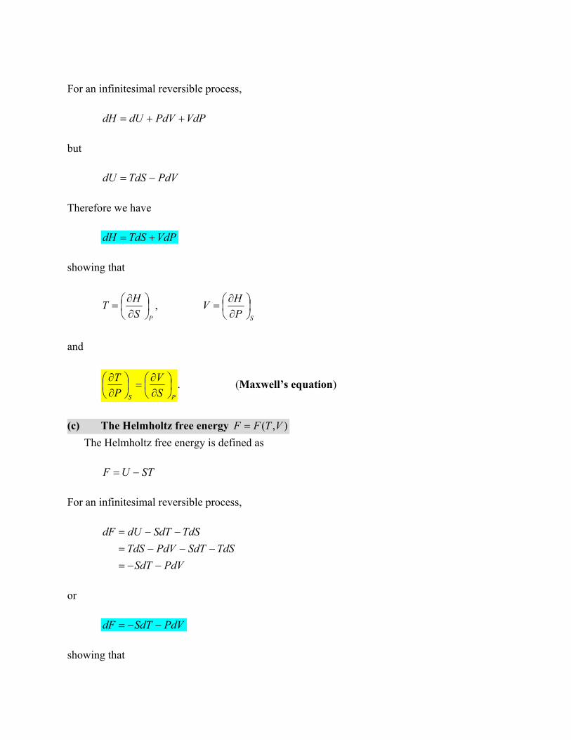
(c) The Helmholtz free energy ),( VTFF

The Helmholtz free energy is defined as

STUF

For an infinitesimal reversible process,

PdVSdT

TdSSdTPdVTdS

TdSSdTdUdF

or

PdVSdTdF

showing that

VT

FS

, TV

FP

VT T

P

V

S

(Maxwell’s equation)

We note that

V

V T

F

TT

T

FTFSTFU ][2

(Gibbs-Helmholtz equation)

(d) The Gibbs free energy ),( PTGG

The Gibbs free energy is defined as

TSHPVFG

For an infinitesimal reversible process,

VdPSdT

TdSSdTVdPTdS

TdSSdTdHdG

or

VdPSdTdG

with

VdPTdSdH ,

showing that

PT

GS

, TP

GV

and

PT T

V

P

S

(Maxwell’s equation)

We note that

PP T

G

TT

T

GTGTSGH

2 (Gibbs-Helmholtz equation)

6. Relations between the derivatives of thermodynamic quantities

(a) First energy equation

PdVTdSdU

PV

ST

PdVTdSVV

U

T

TT

)(

Using the Maxwell’s relation VT T

P

V

S

, we get

PT

PT

V

U

VT

(First energy equation)

which is called the first energy equation. For the ideal gas ( TNkPV B ), we can make a proof of

the Joule’s law.

0

TV

U

In other words, U is independent of V: TCU V (Joule’s law for ideal gas)

(b) Second energy equation

PdVTdSdU

TT

TT

P

VP

P

ST

PdVTdSPP

U

)(

Using the Maxwell’s relation PT T

V

P

S

, we get

TPT P

VP

T

VT

P

U

(second energy equation)

which is called the second energy equation. For an ideal gas,

2( ) 0

T

U R RTT P

P P P

In other words, U is independent of P: TCU V (Joule’s law for ideal gas)

7. Generalized susceptibility

P

PT

V

V

1

; isobaric expansivity

S

ST

V

V

1

; adiabatic expansivity

T

TP

V

V

1

; isothermal compressibility

S

SP

V

V

1

; adiabatic compressibility

8. The ratio V

P

C

C

),(

),(

),(

),(

),(

),(

),(

),(

),(

),(

),(

),(

TV

SV

TP

SP

TP

SP

SV

TV

SV

SP

TP

TV

P

V

P

V

S

T

S

T

or

),(

),(

),(

),(

),(

),(

),(

),(

),(

),(

),(

),(

TV

SV

TP

SP

TP

SP

SV

TV

SV

SP

TP

TV

P

V

P

V

S

T

S

T

or

V

P

V

P

S

T

C

C

T

ST

T

ST

VT

VS

PT

PS

),(

),(

),(

),(

9. Mayer’s relation

(a) Relation

T

VVP

V

P

T

P

TCC

2

The thermodynamics first law:

PdVTdSdU

PP

PT

ST

T

QC

Transforming PC to the variable T and P,

T

VT

V

VTTV

T

TV

TV

T

P

V

P

T

P

V

S

T

S

T

P

V

S

V

P

T

S

V

P

V

P

T

P

V

S

T

S

V

P

VT

PT

VT

PS

PT

PS

T

S

][1

1

),(

),(

),(

),(

),(

),(

Here we use the Maxwell’s relation,

VT T

P

V

S

Thus we get

T

V

VP

V

P

T

P

TT

ST

T

ST

2

or

T

VVP

V

P

T

P

TCC

2

Note that

T

T

P

V

TP

TVTV

TP

V

P

1

),(

),(

1

),(

),(

T

P

V

P

V

T

V

PT

VT

PT

VP

VT

VP

T

P

),(

),(

),(

),(

),(

),(

Then we have

T

P

T

PVP VT

P

V

T

V

TCC 2

2

(b) Relation

T

PVP

P

V

T

V

TCC

2

Similarly, transforming VC to the variable T and V,

T

PT

P

PTTP

T

TP

TP

T

V

P

V

T

V

P

S

T

S

T

V

P

S

P

V

T

S

P

V

P

V

T

V

P

S

T

S

P

V

PT

VT

PT

VS

VT

VS

T

S

][1

1

),(

),(

),(

),(

),(

),(

Using the Maxwell’s relation

PT T

V

P

S

we have

T

P

PV

P

V

T

VT

T

ST

T

ST

2][

or

T

P

T

PVP VT

P

V

T

V

TCC 2

2][

10. Derivative of CV with respect to T (Reif, Blundell)

TV

TV

VTT

V

V

S

TT

V

S

TT

VT

ST

TV

ST

T

ST

VV

C

2

2

][

Using the Maxwell’s relation

VT T

P

V

S

we get

VVVT

V

T

PT

T

P

TT

V

C

2

2

11. Derivative of PC with respect to P (Reif, Blundell)

TP

TP

PTT

P

P

S

TT

P

S

TT

PT

ST

TP

ST

T

ST

PP

C

2

2

][

Using the Maxwell’s relation

PT T

V

P

S

we get

PPPT

P

T

VT

T

V

TT

P

C

2

2

12. Joule-Thomson expansion

P

T

H

T

H

P

H

TP

HP

TP

HT

HP

HT

P

T

),(

),(

),(

),(

),(

),(

Note that

VdPTdSdH

So we get

VT

VT

VP

ST

VdPTdSPP

H

T

T

TT

)(

P

P

PP

C

T

ST

VdPTdSTT

H

)(

Thus we have

][1

VT

VT

CP

T

TPH

REFERENCES

L.D. Landau and E.M. Lifshitz, Statistical Physics, 3rd edition, revised and enlarged (Pergamon,

1980).

F. Reif, Fundamentals of Statistical and Thermal Physics (McGraw-Hill, 1965).

S. Blundel and K. Blundel, Concepts of Thermal Physics (Oxford, 2015).

APPENDIX

Stokes theorem and conservative force

1 Conservative force

1.1 Path integral

The work done by a conservative force on a particle moving between any two points is

independent of the path taken by the particle.

321 Pathc

Pathc

Pathc ddd rFrFrF

for any path connecting two points A and B.

1.2 Path integral along the closed path

The work done by a conservative force on a particle moving through any closed path is zero.

(A closed path is one for which the beginning point and the endpoint are identical).

0 rF dc , for any closed path

2 Potential energy U

The quantity rF dc can be expressed in the form of a perfect differential

rF dWdU cc

where the function U(r) depends only on the position vector r and does not depend explicitly on

the velocity and time. A force Fc is conservative and U is known as the potential energy.

)()( BUAUdUd

B

A

B

A

c rF

which does not depend on the path of integration but only on the initial and final positions. It is

clear that the integral over a closed path is zero

0 rF dc (1)

which is a different way of saying that the force field is conservative

Using Stoke’s theorem;

For any vector A,

aArA dd )( .

Since

0)( aFrF dd cc

we have

0 cF , (2)

where is a differential operator called del or nabla. The operator can be written in n terms of

the Cartesian components x, y, z in the form

zyx

kji ˆˆˆ

In this case, Fc can be expressed by

Uc F

or

z

U

y

U

x

Uc ,,F

which leads to the relation

z

F

x

F

y

F

z

F

x

F

y

F

cxcz

czcy

cycx

.

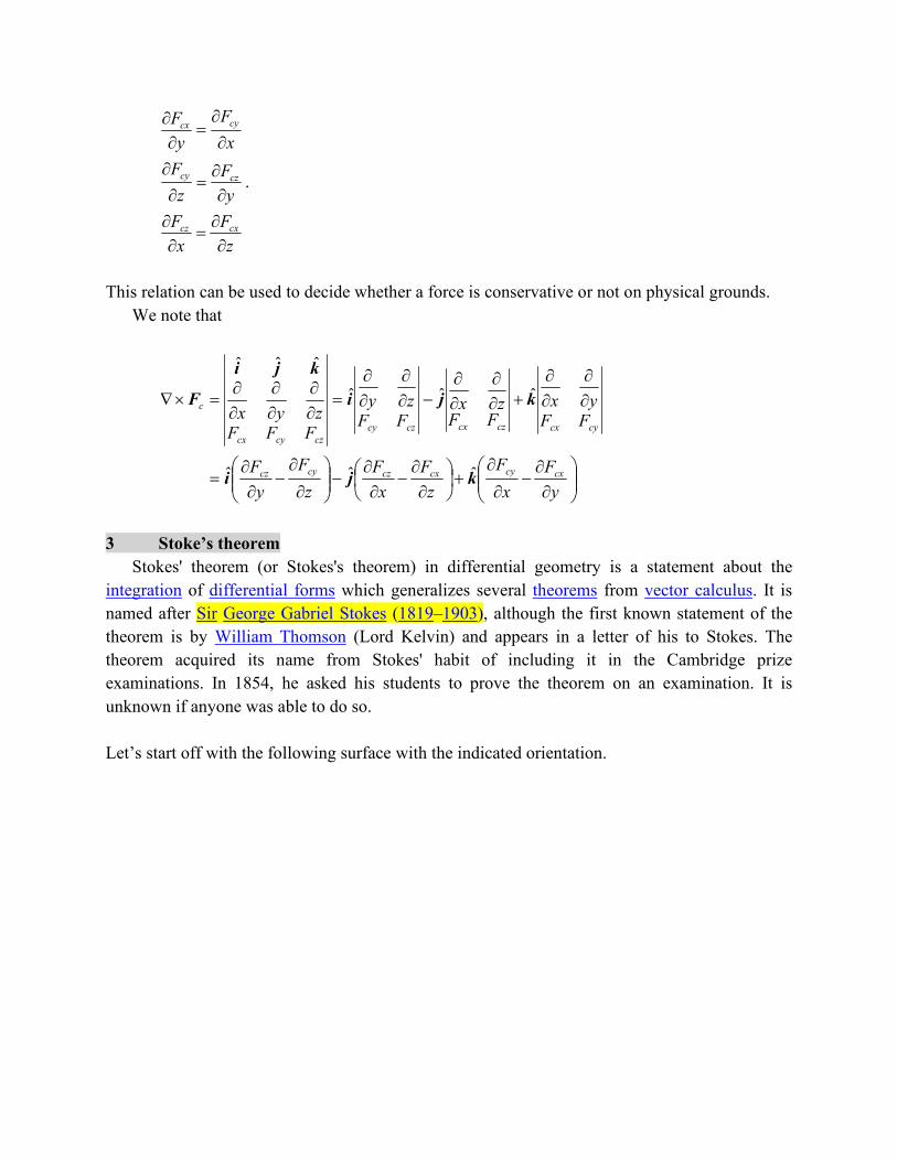
This relation can be used to decide whether a force is conservative or not on physical grounds.

We note that

y

F

x

F

z

F

x

F

z

F

y

F

FFyx

FFzx

FFzy

FFFzyx

cxcycxczcycz

cycxczcxczcy

czcycx

c

kji

kji

kji

F

ˆˆˆ

ˆˆˆ

ˆˆˆ

3 Stoke’s theorem

Stokes' theorem (or Stokes's theorem) in differential geometry is a statement about the

integration of differential forms which generalizes several theorems from vector calculus. It is

named after Sir George Gabriel Stokes (1819–1903), although the first known statement of the

theorem is by William Thomson (Lord Kelvin) and appears in a letter of his to Stokes. The

theorem acquired its name from Stokes' habit of including it in the Cambridge prize

examinations. In 1854, he asked his students to prove the theorem on an examination. It is

unknown if anyone was able to do so.

Let’s start off with the following surface with the indicated orientation.

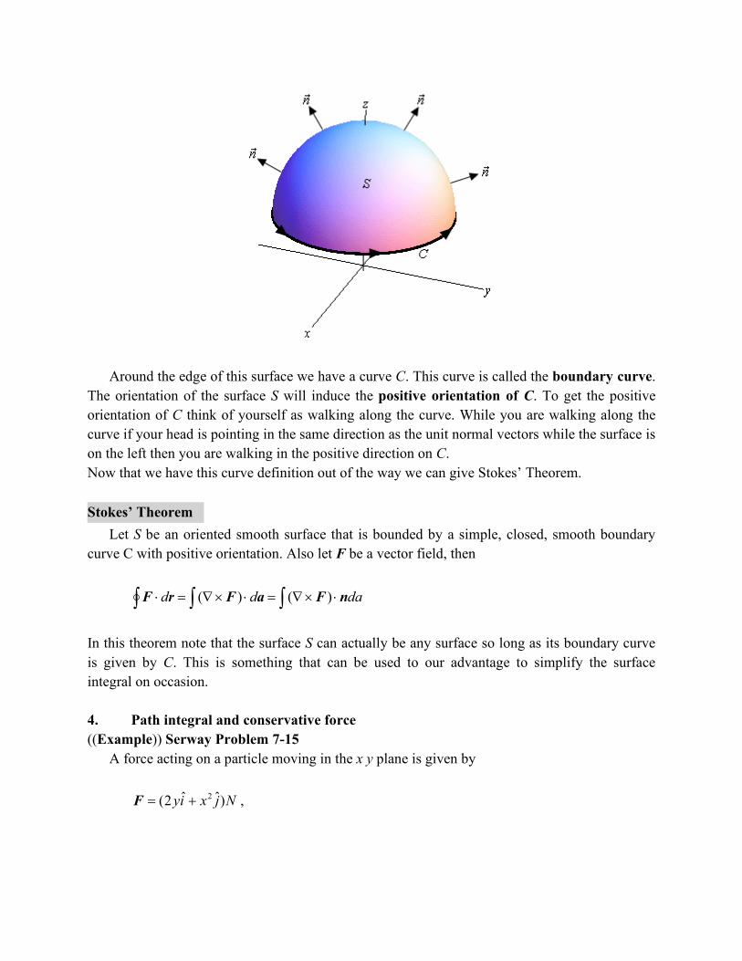
Around the edge of this surface we have a curve C. This curve is called the boundary curve.

The orientation of the surface S will induce the positive orientation of C. To get the positive

orientation of C think of yourself as walking along the curve. While you are walking along the

curve if your head is pointing in the same direction as the unit normal vectors while the surface is

on the left then you are walking in the positive direction on C.

Now that we have this curve definition out of the way we can give Stokes’ Theorem.

Stokes’ Theorem

Let S be an oriented smooth surface that is bounded by a simple, closed, smooth boundary

curve C with positive orientation. Also let F be a vector field, then

dadd nFaFrF )()(

In this theorem note that the surface S can actually be any surface so long as its boundary curve

is given by C. This is something that can be used to our advantage to simplify the surface

integral on occasion.

4. Path integral and conservative force

((Example)) Serway Problem 7-15

A force acting on a particle moving in the x y plane is given by

Njxiy )ˆˆ2( 2F ,

where x and y are in meters. The particle moves from the origin to a final position having

coordinates x = 5.00 m and y = 5.00 m as in Fig. Calculate the work done by F along (a) OAC,

(b) OBC, (c) OC. (d) Is F conservative or nonconservative? Explain.

((Solution))

dyxydxdyFdxFd yx

22 rF

Path OAC

On the path OA; x = 0 – 5, y = 0; jx ˆ2F and dy = 0.

0. A

O

drF

On the path AC; x = 5, y = 0 - 5; jj ˆ25ˆ52 F

5

0

12525. dyd

C

A

rF

Then we have

Jd

C

O

125. rF for the path OAC

Path OBC

On the path OB; x = 0, y = 0 - 5;

ydxd 2 rF and dx = 0

or

0B

O

drF

On the path BC; x = 0 - 5, y = 5; dxydxd 102 rF

5

0

5010dxd

C

B

rF

Then we have

50C

O

drF J for the path OBC

Path OC

x = t, y = t for t = 0 – 5.

dtttdtttdtdyxydx )2(22 222

Jdtttd

C

O3

200

2

52

3

125)2(

25

0

2 rF

for the path OC line. Then the force is non-conservative.

((Note))

Nxy )ˆˆ2( 2 jiF

xx

F

y

F

y

x

2

2

This implies that the force is not conservative.