Evolution of chemical abundances in active and quiescent ...
154
Universit ` a degli studi di Trieste Facolt` a di Scienze Matematiche, Fisiche e Naturali Dottorato di Ricerca in Fisica - XX Ciclo Evolution of chemical abundances in active and quiescent spiral bulges Settore scientifico-disciplinare: FIS/05 ASTRONOMIA E ASTROFISICA Dottorando Coordinatore del Collegio dei Docenti Silvia Kuna Ballero Prof. Gaetano Senatore, Universit` a di Trieste Tutore Prof. Francesca Matteucci, Universit` a di Trieste Relatore Prof. Francesca Matteucci, Universit` a di Trieste A.A. 2006/2007
Transcript of Evolution of chemical abundances in active and quiescent ...

Universita degli studi di Trieste
Facolta di Scienze Matematiche, Fisiche e Naturali
Dottorato di Ricerca in Fisica - XX Ciclo
Evolution of chemical abundances
in active and quiescent spiral bulges
Settore scientifico-disciplinare: FIS/05 ASTRONOMIA E ASTROFISICA
Dottorando Coordinatore del Collegio dei Docenti
Silvia Kuna Ballero Prof. Gaetano Senatore, Universita di Trieste
Tutore
Prof. Francesca Matteucci, Universita di Trieste
Relatore
Prof. Francesca Matteucci, Universita di Trieste
A.A. 2006/2007


This is dedicated to Dero

Contents
1 Introduction 1
1.1 Galactic bulges: definition and properties . . . . . . . . . . . . . . . . . . 1
1.2 Scenarios of bulge formation and evolution . . . . . . . . . . . . . . . . . 5
1.3 Bulges and Seyfert galaxies . . . . . . . . . . . . . . . . . . . . . . . . . 10
1.4 Aims and plan of the thesis . . . . . . . . . . . . . . . . . . . . . . . . . 12
2 The chemical evolution model for bulges 15
2.1 The stellar birthrate . . . . . . . . . . . . . . . . . . . . . . . . . . . . . 15
2.2 The equation of chemical evolution . . . . . . . . . . . . . . . . . . . . . 16
2.3 The starting model . . . . . . . . . . . . . . . . . . . . . . . . . . . . . . 17
2.4 The new chemical evolution model . . . . . . . . . . . . . . . . . . . . . 19
2.4.1 Implementation of the wind . . . . . . . . . . . . . . . . . . . . . 21
3 Formation and evolution of the Milky Way bulge 23
3.1 Model parameters . . . . . . . . . . . . . . . . . . . . . . . . . . . . . . . 23
3.2 Observations of abundances in the Galactic bulge . . . . . . . . . . . . . 24
3.2.1 Metallicity distribution . . . . . . . . . . . . . . . . . . . . . . . . 25
3.2.2 α-elements and carbon . . . . . . . . . . . . . . . . . . . . . . . . 27
3.2.3 Nitrogen . . . . . . . . . . . . . . . . . . . . . . . . . . . . . . . . 29
3.3 Results . . . . . . . . . . . . . . . . . . . . . . . . . . . . . . . . . . . . . 33
3.3.1 The supernova rates . . . . . . . . . . . . . . . . . . . . . . . . . 33
3.3.2 The metallicity distribution of the bulge giants . . . . . . . . . . . 35
3.3.3 Evolution of the abundance ratios . . . . . . . . . . . . . . . . . . 40
3.4 Summary and conclusions . . . . . . . . . . . . . . . . . . . . . . . . . . 51
4 O and Mg evolution in the Galactic bulge and solar neighbourhood 55
4.1 Mass loss and stellar yields . . . . . . . . . . . . . . . . . . . . . . . . . . 55
II CONTENTS
4.2 Evidence for metallicity-dependent O yields . . . . . . . . . . . . . . . . 57
4.3 The chemical evolution models . . . . . . . . . . . . . . . . . . . . . . . . 61
4.4 Results . . . . . . . . . . . . . . . . . . . . . . . . . . . . . . . . . . . . . 62
4.4.1 [O/Mg] vs. [O,Mg/H] . . . . . . . . . . . . . . . . . . . . . . . . . 62
4.4.2 [O/Fe] vs. [Fe/H] . . . . . . . . . . . . . . . . . . . . . . . . . . . 67
4.5 Summary and conclusions . . . . . . . . . . . . . . . . . . . . . . . . . . 69
5 Universal or environment-dependent IMF? 71
5.1 The issue of the IMF . . . . . . . . . . . . . . . . . . . . . . . . . . . . . 71
5.2 Model results . . . . . . . . . . . . . . . . . . . . . . . . . . . . . . . . . 73
5.2.1 Constraining yields for very massive stars . . . . . . . . . . . . . . 75
5.2.2 The effect of other evolutionary parameters . . . . . . . . . . . . 78
5.2.3 Results for M31 . . . . . . . . . . . . . . . . . . . . . . . . . . . . 78
5.2.4 Discussion . . . . . . . . . . . . . . . . . . . . . . . . . . . . . . . 80
5.3 Summary and conclusions . . . . . . . . . . . . . . . . . . . . . . . . . . 81
6 Chemical evolution of Seyfert galaxies and bulge photometry 83
6.1 The co-evolution of AGNs and spheroids . . . . . . . . . . . . . . . . . . 83
6.2 Observations of abundances in QSOs and Seyfert galaxies . . . . . . . . . 85
6.3 Building models for other bulges . . . . . . . . . . . . . . . . . . . . . . . 88
6.4 Photometry of bulges . . . . . . . . . . . . . . . . . . . . . . . . . . . . . 89
6.5 Energetics of the interstellar medium . . . . . . . . . . . . . . . . . . . . 90
6.5.1 The binding energy . . . . . . . . . . . . . . . . . . . . . . . . . . 90
6.5.2 Black hole accretion and feedback . . . . . . . . . . . . . . . . . . 94
6.6 Results . . . . . . . . . . . . . . . . . . . . . . . . . . . . . . . . . . . . . 95
6.6.1 Mass loss and energetics . . . . . . . . . . . . . . . . . . . . . . . 95
6.6.2 Star formation rate . . . . . . . . . . . . . . . . . . . . . . . . . . 98
6.6.3 Black hole masses and luminosities . . . . . . . . . . . . . . . . . 100
6.6.4 Metallicity and elemental abundances . . . . . . . . . . . . . . . . 104
6.6.5 Bulge colours and colour-magnitude relation . . . . . . . . . . . . 114
6.7 Summary and conclusions . . . . . . . . . . . . . . . . . . . . . . . . . . 120
7 Concluding remarks 123
7.1 Summary . . . . . . . . . . . . . . . . . . . . . . . . . . . . . . . . . . . 123
7.2 Future perspectives . . . . . . . . . . . . . . . . . . . . . . . . . . . . . . 126

CONTENTS III
A The disk gravitational energy contributions 127
Bibliography 129
Acknowledgements 147

Chapter 1
Introduction
”In the beginning the Universe was created. This has made a lot
of people very angry and been widely regarded as a bad move.”
(Douglas Adams)
1.1 Galactic bulges: definition and properties
There is not a general consensus on what is meant for a bulge in astronomy. According to
the most general definition, any spheroidal stellar system is a bulge, i.e. this definition
includes both elliptical galaxies and the spheroidal stellar components located at the
centre of spiral galaxies. To further confuse the reader, the latter show a bimodality
of properties, therefore spiral bulges are divided accordingly into true (or classical)
bulges and pseudobulges (Kormendy & Kennicutt 2004). These two subclasses have
very different evolutionary histories. While the former are thought to form very rapidly
and almost independently of the disk, the latter are most probably built slowly by
disk material; this is suggested by the similarity of their features to those of the disk,
contrarily to classical bulges. Our work will only concern classical bulges of spiral
galaxies.
Spiral bulges usually possess metallicity1, photometric and kinematic properties that
separate them from all the other components (thin disk, thick disk and halo) of spirals,
whereas they show a broad similarity to elliptical galaxies and among themselves. Their
stellar angular momentum distribution clearly separates them from the disk components,
which are fully rotationally supported, and suggests that the halo and bulge are kine-
1We define as metallicity Z the abundance fraction by mass of all the chemical species heavier
than 4He.

2 1.1 Galactic bulges: definition and properties
Figure 1.1: A sketch of the structure of the Milky Way: the stellar halo, bulge, thick and
thin disk are indicated together with the mean metallicity of the stars in each galactic
component. The galactocentric distance of the Sun and the dimension of the optical
disk are shown at the bottom.
matically linked as different parts of the same spheroid. Whitford (1978) and Maraston
et al. (2003) found a significant similarity of the integrated light of the Galactic bulge
to that of elliptical galaxies and other spiral bulges. Moreover, bulges and ellipticals are
located in the same region of the Fundamental Plane (Falcon-Barroso et al. 2002), i.e. a
plane in the space defined by the effective radius Re, the mean surface brightness within
Re (Σe) and the central velocity dispersion σ (Djorgovski & Davies 1987; Bender et al.
1992; Burstein et al. 1997). The scaling relation represented by the Fundamental Plane
is very tight. The small scatter shown by ellipticals around the Fundamental Plane is
interpreted as an evidence of a highly synchronised formation of this type of galaxies,
and is naturally explained by a scenario where ellipticals are formed at high redshift.
Given these analogies, this is a first evidence that bulges are old systems which formed
on a quite short timescale.
More direct evidence of the age of bulges comes from photometrical studies of our
own bulge. The presence of RR Lyrae variables (Lee 1992; Alard 1996) shows that
there is at least one component of age comparable to that of the oldest known stars
(i.e. those in the globular clusters of the halo). Terndrup (1988) first argued for a

Chapter 1. Introduction 3
globular cluster-like nature of the bulge population. From colour-magnitude diagrams
of M giants, he derived old ages (τturn−off = 11±3 Gyr) and concluded that bulge stars
formed almost simultaneously and that there has not been star formation for the last
5 Gyrs. From the analysis of the bulge horizontal branch stars, Lee (1992) found that
the oldest stars in the bulge are older than the oldest halo stars by ∼ 1 Gyr, and an
analogous conclusion was reached also by Ortolani et al. (1995). Recently, Kuijken &
Rich (2002) showed that when the bulge field is decontaminated from disk foreground
stars by proper motion cleaning or statistical subtraction, the remaining population of
stars is indistinguishable from that of an old metal rich globular cluster.
This seems to be at variance with the discovery of a sub-population confined to the
most central regions of the bulge, whose age is estimated to be a few Gyrs (e.g. Harmon
& Gilmore 1988, Holtzman et al. 1993; van Loon et al. 2003). However, we must
consider that bulges are not isolated systems, and that many of them are influenced by
the presence of a bar which can drive disk gas to the centre and give rise to secondary
episodes of star formation extending out to a few parsecs from the centre. In any case,
the younger population will contribute a minor fraction of the bulge stellar population
(∼ 10 − 20%).
Chemical abundances provide an independent way to estimate the formation history
of bulges. Before discussing the abundances in the gas or in stars, we define the bracket
notation for abundance ratios. If A and B are two chemical elements and XA, XB their
respective abundance fractions by mass, then
[A/B] = log(XA/XB)gas,star − log(XA/XB) (1.1)
where the subscript refers to the Sun. These abundances are measured in units of
dex (decimal exponential).
Deriving accurate and detailed chemical abundances for stars in the Galactic bulge is
not an easy task, since the observations along the line-of-sight to the bulge are hampered
by dust extinction and reddening which, on the Galactic plane, are very large. However,
it is possible to perform successful observations in some low-extinction windows, among
which the so-called Baade’s Window, a region with l = 1, b = −4.
By observing K giants in the Baade’s window with low-resolution spectroscopy, Rich
(1988) measured a wide range of [Fe/H] (from −1.5 to +1.0 dex) with a mean value
of +0.3 dex. Later, McWilliam & Rich (1994) re-calibrated these data with higher-
resolution measurements and found values for [Fe/H] systematically lower by 0.25− 0.3
dex. This result was confirmed by Sadler et al. (1996) for a sample of M and K giants

4 1.1 Galactic bulges: definition and properties
in the bulge, and more recently by Ramırez et al. (2000). The overestimation of Rich
(1988) was partly due to blending of lines, and partly to the assumption [Mg/Fe] = 0.0
employed to derive [Fe/H] values from the magnesium index Mg2, whereas the ratios
of α-elements (O, Ne, Mg, Si, S, Ca, Ti) over Fe in the bulge are enhanced with re-
spect to the sun. The α-enhancement is a signature of fast star formation history, since
α-elements are produced by Type II supernovae, contrarily to Fe, whose main contrib-
utors are Type Ia supernovae. The difference in the timescales for the occurrence of
Type Ia and Type II supernovae produces a time delay in the Fe production relative to
the α-elements (time delay model : Tinsley 1979; Greggio & Renzini 1983; Matteucci &
Greggio 1986). McWilliam & Rich (1994) and Sadler et al. (1996) found a certain degree
of α-enhancement, but the situation remained unclear until Barbuy (1999) showed over-
abundances for most of the α-elements observed in stars belonging to the bulge globular
clusters NGC 6553 and NGC 6528. Subsequent high-resolution (R ∼ 45000 − 60000)
spectroscopic works, both in in low-extinction optical windows (e.g. McWilliam & Rich
2004; Zoccali et al. 2006; Lecureur et al. 2007; Fulbright et al. 2007), or in the infrared
(Origlia et al. 2005; Rich & Origlia 2005) firmly established this trend for α-elements.
These recent data were the basis for the development of our bulge chemical evolution
model and will be extensively discussed in §3.2.
Another way to obtain an estimate of the metallicity distribution of bulge giants
other than spectroscopy is by means of photometry, and namely by the analysis of
specific features of the colour-magnitude diagram. The mean de-reddened colour and
colour dispersion of the red giant branch can be matched with empirical red giant
branch templates to determine the global metal abundance and its dispersion, and to
set constraints on the bulge age as well. Thus, Zoccali et al. (2003) essentially confirmed
a wide range in [Fe/H] and an age of ∼ 10 Gyr for the stellar population residing in
the bulge, whereas Sarajedini & Jablonka (2005) suggest that, since the differences in
the metallicity distributions of the Milky Way and M31 halos find no correspondence in
those of their bulges, the bulk of the stars in the bulges of both galaxies must have been
in place before any accretion event, that might have occurred in the halo, could have
any influence on them. This conclusion supports a common scenario for the formation
of bulges.
It is not clear whether there is a metallicity gradient in the Galactic bulge. Minniti
et al. (1995) measured a gradient within the inner 2 kiloparsecs of the Galaxy, although
the spread in metal abundances at any given galactocentric distance is large. If con-

Chapter 1. Introduction 5
firmed, the presence of a metallicity gradient together with a correlation between stellar
abundances and kinematics would be a strong signature of a fast dissipative collapse,
as opposed to dissipationless stellar merging or formation through inflow of material
expelled from the disk.
1.2 Scenarios of bulge formation and evolution
The first modern model for the formation of the Milky Way was proposed by Eggen,
Lynden-Bell & Sandage (1962). In their scenario, the halo and the bulge form through
a rapid “monolithic” collapse within only 108 years, approximately 1010 years ago, when
extended and nearly spherical protogalactic gas clouds cooled and condensed out of the
dark matter halo. This collapse initiated the formation of the Galaxy as a whole. The
lowest angular momentum gas fell into the centre and formed the bulge; fast star for-
mation in an initial burst and subsequent enrichment can explain the bulge metallicity.
The high angular momentum gas collapsed later and formed the disk. In this context,
the bulge is essentially the oldest component of a spiral galaxy (“old-bulge” scenario),
and is treated as a miniature elliptical. Eggen et al. (1962) also argued that the ob-
served highly non-circular motions of halo stars can be understood only if the collapse
was rapid and lasted no longer than 2 × 10⁸ years.
As a cause of the rapid collapse in this simple scenario a correlation among metal-
licity, age and kinematics and a metallicity gradient in the halo is expected. When
investigating the metallicity of globular clusters of the outer halo, Searle & Zinn (1978)
did not find any significant gradient. Motivated through these observations, they pro-
posed a more chaotic origin of the Galactic halo, in which the central regions form first.
In their scenario, the outer halo is formed by inhomogeneous coalescence of transient
extant protogalactic stellar systems during an extended period of time after the col-
lapse of the central region is completed. Within this scenario, the bulge is again formed
early in the history of the Galaxy. The idea of a bulge consisting of material coming
from satellite galaxies was further adopted by Schweizer & Seitzer (1988) who observed
sharped-edge ripples in disk galaxies and concluded that they consisted of extraneous
matter acquired through mass transfer from neighbour galaxies. They also suggested
that such intruders would end up in the bulge, thus giving rise to episodic growth.
More recent models of bulge formation were developed who assumed accretion of stellar
satellites (e.g. Aguerri et al. 2001). However, Wyse (1998) showed that the metallicity

6 1.2 Scenarios of bulge formation and evolution
distribution in our Galaxy is not consistent with a picture where the bulge is formed via
accretion of satellites. There is now additional evidence that the bulge is not formed
by satellites similar to those observed at the present day in the halos of the Milky Way
and M31: McWilliam et al. (2003) find a systematically decreased abundance of Mn
in the Galactic bulge, compared to stars in the Sgr dwarf spheroidal. So, even though
Sgr does in principle reach high metallicities, its detailed chemistry is different (see also
Venn et al. 2004, Monaco et al. 2007).
In the framework of the Eggen, Lynden-Bell and Sandage (1962) scenario, early
numerical one-zone, closed-box2 models for ellipticals, adopting the instantaneous recy-
cling approximation3 (Arimoto & Yoshii 1986), were able to produce the observed wide
abundance range. The incorporation of yields from Type Ia and Type II supernovae and
detailed stellar lifetimes into these models allowed to make more extensive predictions.
In this way, Matteucci & Brocato (1990) predicted that the [α/Fe] ratio for some ele-
ments (O, Si and Mg) should be supersolar over almost the whole metallicity range, in
analogy with the halo stars, as a consequence of assuming a fast bulge evolution which
involved rapid gas enrichment in Fe mainly by Type II supernovae. At that time, no
data were available for detailed chemical abundances; the predictions of Matteucci &
Brocato (1990) were later confirmed for a few α-elements (Mg, Ti) by the observations
of McWilliam & Rich (1994), whereas for other elements (e.g. O, Ca, Si) the observed
trend looked different. Other discrepancies regarding the Mg overabundance came from
the observations of Sadler et al. (1996).
In order to better assess these points, Matteucci, Romano & Molaro (1999) modelled
the behaviour of a larger set of abundance ratios, by means of a detailed chemical
evolution model whose parameters were calibrated so that the metallicity distribution
observed by McWilliam & Rich (1994) could be fitted. They predicted the evolution of
several abundance ratios that were meant to be confirmed or disproved by subsequent
observations, namely that α-elements should in general be overabundant with respect
to Fe, but some (e.g. Si, Ca) less than others (e.g. O, Mg), due to the fact that they are
partly synthesised in Type Ia supernovae, and that the [12C/Fe] ratio should be solar at
2In a closed-box galactic model, all the gas is present at the beginning; no infall or outflow occur.
3The instantaneous recycling approximation consists in the assumptions that all stars with
M < 1M live forever, whereas all stars with M > 1M die immediately. This approximation al-
lows to neglect stellar lifetimes and simplify the equations of chemical evolution. However, while the
first assumption is reasonable, the second one leads to model incorrectly the evolution of elements which
contribute to the enrichment of the interstellar medium at later times (e.g. Fe).
Chapter 1. Introduction 7
all metallicities. They concluded that an initial mass function flatter (x = 1.1 − 1.35;
see §2.1) than that of the solar neighbourhood is needed for the metallicity distribution
of McWilliam & Rich (1994) to be reproduced, and that a much faster evolution than in
the solar neighbourhood and faster than in the halo (see also Renzini, 1993) is necessary
as well.
Molla et al. (2000) proposed a multiphase model in the context of the dissipative
collapse scenario of the Eggen, Lynden-Bell & Sandage (1962) picture. They suppose
that the bulge formation occurred in two main infall episodes, the first from the halo to
the bulge, on a timescale τH = 0.7 Gyr (longer than that proposed by Matteucci et al.
1999), and the second from the bulge to a so-called core population in the very nuclear
region of the Galaxy, on a timescale τB τH . The three zones (halo, bulge, core)
interact via supernova winds and gas infall. They concluded that there is no need for
accretion of external material to reproduce the main properties of bulges and that the
analogy to ellipticals is not justified. Because of their rather long timescale for the bulge
formation, these authors did not predict a noticeable difference in the trend of the [α/Fe]
ratios but rather suggested that they behave more likely as in the solar neighbourhood
(contrary to the first indications of α-enhancement by McWilliam & Rich 1994).
Ferreras, Wyse & Silk (2003) tried to fit the stellar metallicity distributions of K gi-
ants measured by Sadler et al. (1996), Ibata & Gilmore (1995) and Zoccali et al. (2003),
which are pertinent to different bulge fields, by means of a model of star formation and
chemical evolution. Their model assumes a Schmidt law similar to that of the disk, and
simple recipes with a few parameters controlling infall and continuous outflow of gas.
They explored a large range in the parameter space and conclude that timescales longer
than ∼ 1 Gyr must be excluded at the 90% confidence level, regardless of which field is
being considered.
A more recent model was proposed by Costa et al. (2005), in which the best fit to the
observations relative to planetary nebulae is achieved by means of a double infall model.
An initial fast (0.1 Gyr) collapse of primordial gas is followed by a supernova-driven
mass loss and then by a second, slower (2 Gyr) infall episode, enriched by the material
ejected by the bulge during the first collapse. Costa et al. (2005) claim that the mass
loss is necessary to reproduce the abundance distribution observed in planetary nebulae,
and because the predicted abundances would otherwise be higher than observed. With
their model, they are able to reproduce the trend of [O/Fe] abundance ratio observed
by Pompeia et al. (2003) and the data of nitrogen versus oxygen abundance observed

8 1.2 Scenarios of bulge formation and evolution
by Escudero & Costa (2001) and Escudero et al. (2004). It must be noted however
that Pompeia et al. (2003) obtained abundances for “bulge-like” dwarf stars. This
“bulge-like” population consists of old (∼ 10 − 11 Gyr), metal-rich nearby dwarfs with
kinematics and metallicity suggesting an inner disk or bulge origin and a mechanism
of radial migration, perhaps caused by the action of a Galactic bar. However, the
birthplace of these stars is not certain (and in the discussion of our model we shall omit
these data from our model, and only consider those stars for which membership in the
present day bulge is secure). Moreover, as we shall see, the use of nitrogen abundance
from planetary nebulae is questionable, since N is known to be also synthesised by their
progenitors and therefore it might not be the pristine one.
A short formation timescale for the bulge is also suggested on theoretical grounds by
Elmegreen (1999), who argued that the potential well of the Galactic bulge is too deep
to allow self-regulation and that most of the gas must have been converted into stars
within a few dynamical timescales.
Not all models of the bulge support the conclusions of a fast formation and evolution.
In the hierarchical clustering scenario (Kauffmann 1996) the bulges form through violent
relaxation and destruction of disks in major mergers. The stars of the destroyed disk
build the bulge, and subsequently the disk has to be rebuilt. This implies that late type
spirals should have older bulges than early types, since the build-up of a large disk needs
time during which the galaxy is allowed to evolve undisturbed. This is not confirmed by
observations, as well as the high metallicity and the narrow age distribution observed
in bulges of local spirals are not compatible with a merger origin of these objects (see
Wyse 1999, and references therein).
Samland et al. (1997) developed a self-consistent chemo-dynamical model for the
evolution of the Milky Way components starting from a rotating protogalactic gas cloud
in virial equilibrium, that collapses owing to dissipative cloud-cloud collisions. They
found that self-regulation due to a bursting star formation and subsequent injection
of energy from Type II supernovae lead to the development of “contrary flows”, i.e.
alternate collapse and outflow episodes in the bulge. This causes a prolonged star
formation episode lasting over ∼ 4 × 10⁹ yr. They included stellar nucleosynthesis of
O, N and Fe, but claim that gas outflows prevent any clear correlation between local
star formation rate and chemical enrichment. With their model, they could reproduce
the oxygen gradient of H ii regions in the equatorial plane of the Galactic disk and the
metallicity distribution of K giants in the bulge (Rich 1988), field stars in the halo and G

Chapter 1. Introduction 9
dwarfs in the disk, but they did not make predictions about the evolution of abundance
ratios in the bulge.
Finally, there is another class of scenarios for the bulge formation, which investigate
the outcome of the secular evolution of disks. In this context, bulges are assumed to
be the result of instabilities that either drive gas to the galactic centre, e.g. through
the action of a stellar bar or due to gravitational instabilities of the spiral structure, or
lead to the fragmentation and partial disruption of the internal disk with subsequent re-
buildup. Indications of bulges unaccounted for by the “old-bulge” scenario include: the
existence of box-shaped or peanut-shaped bulges and triaxiality (Bertola et al. 1991);
observations of bulges with velocity dispersions (Kormendy 1982) and colours (Balcells
& Peletier 1994) close to those of disks; and deviations from the de Vaucouleur’s r1/4
profile (Wainscoat et al. 1989).
The idea of secular evolution developed in the 80’s, and was prompted by N -body
simulations; Combes & Sanders (1981) first demonstrated that the vertical thickening
of a stellar bar can produce a bulge-like object in the centre of the disk. This conclusion
was later confirmed and refined by Pfenniger & Norman (1990) and Hasan et al. (1993):
a barred potential in a flat disk can lead to heating of the stellar component in the
centre, with the formation of a bulge-like structure. However, the bulges produced by
means of this mechanism are small compared to the disk, and multiple minor accretion
events have to be invoked to account for the big bulges of early-type spirals. Other
examples of models assuming secular evolution of disks are those of Friedly & Benz
(1993, 1995), where dissipation can lead to the destruction of the stellar bar producing
a bulge component. The gravitational torque induced by the bar causes an angular
momentum redistribution in the gas phase leading to inflow to the centre. The fuelling
results in an intermediate starburst episode of duration ≈ 108 years. The central mass
accumulation then weakens or destroys the bar, possibly leading to a bulge (Norman et
al. 1996). On the other side, Noguchi (1999) proposed a model of unstable disk which
forms clumps. These clumps then merge, fall to the centre and build a massive bulge.
Immeli et al. (2004) investigated the role of cloud dissipation in the formation and
dynamical evolution of star-forming gas-rich disks by means of a 3-D chemo-dynamical
model including a dark matter halo, stars and a two-phase interstellar medium with
stellar feedback. They found that the galaxy evolution proceeds very differently de-
pending on whether the gas disk or the stellar disk first becomes unstable. This in turn
depends on how efficiently the cold cloud medium can dissipate its kinetic energy. If

10 1.3 Bulges and Seyfert galaxies
the cold gas cools efficiently and drives the instability, the disk fragments and develops
a number of massive clumps of gas and stars which spiral to the centre, where they
merge, thus forming the bulge at relatively early times. A starburst takes place which
gives rise to enhanced [α/Fe] values. This picture corresponds to the model of Noguchi
(1999). On the other hand, if dissipation occurs at a lower rate, stars form in the disk
in a more quiescent fashion and the instability occurs at a much later time, when the
stellar surface density has become sufficiently high. A stellar bar forms which funnels
gas into the centre, then evolves into a bulge at late times. The stars of a bulge formed
in this way keep trace of a more extended star formation history and thus show lower
[α/Fe]. This scenario resembles those of Combes & Sanders (1981) and Pfenniger &
Norman (1990), and seems to be excluded by the recent measurements of Zoccali et al.
(2006) and Lecureur et al. (2007).
We do not exclude that such mechanisms actually occur; however, in our view, struc-
tures fully resulting from the secular evolution of disks must be considered as pseudo-
bulges and not classical bulges. Secular processes can also account for the minority
of young stars found in the very centre of our galaxy; but the chemistry and stellar
ages require that the bulk of bulge stars formed early and self-enriched rapidly (see also
Renzini 1999).
1.3 Bulges and Seyfert galaxies
Active Galactic Nuclei (AGNs) are a class of astrophysical objects of peculiar interest.
They produce extremely high luminosities (up to 104 times the luminosity of a typical
galaxy), and their continuum emission can emerge over up to 13 orders of magnitude,
i.e. they have a rather flat broadband continuum spectrum. So, contrarily to normal
galaxies, for active galaxies (i.e. the galaxies which host an AGN) the emitted radia-
tion is not approximately the sum of the energy radiated by the stars which form them;
there must be a non-thermal component. Many of them show strong and fast variability,
which points to an energy source confined in tiny volumes ( 1 pc3). The most popular
scenario to explain these features is accretion onto a relativistically deep gravitational
potential; the characteristics of AGN emission make black holes the most probable can-
didate (Salpeter 1964). This hypothesis is supported by the detection of supermassive
black holes at the centre of the majority of spheroids (ellipticals and bulges), with masses
MBH & 106M
Chapter 1. Introduction 11
Because their high luminosities and distinctive spectra make them relatively easy
to pick out, AGNs are disproportionately represented among the known high-redshift
sources. Most of them show very prominent emission lines; this makes AGN spectra
stand in great contrast to the spectra of most stars and galaxies, where lines are generally
relatively weak and predominantly in absorption. The emission lines that we see show
a broad similarity among different objects (mainly Lyα, Balmer lines, the C iv 1549
doublet, [O iii] 5007, the Fe Kα X-ray line and others). However, there is a split in
the line width distribution: In some objects many lines have broad wings extending out
several thousand km/s (broad emission lines), whereas in others the line width never
exceeds a few hundred km/s (narrow emission lines). The forbidden lines are only found
within the latter. The mechanism which produces emission lines is photoionization by
the AGN continuum, and the sharp bimodality of emission lines indicates the existence
of two distinct regions with specific cloud properties. The broad line region basically
consists of clumps of gas with density higher than the environmental medium, whose
distance from the ionising source ranges from ∼0.01 to a few pc; their line width is
mainly ascribed to orbital motions. The narrow line region is instead a lower-density
medium located much farther out (several hundred pc).
It is also apparent that AGNs often have absorption features which in general are
much narrower than the emission lines. While broad absorption lines are strongly asso-
ciated to the nuclear region and are thought to be produced by resonance line scattering
in outflowing gas, many of the narrow absorption lines arise from material unassociated
with the AGN, and which lies along the line of sight. However, the detection of intrinsic
narrow absorption lines can be particularly helpful to infer AGN chemical abundances,
since the atomic physics of absorption lines are much simpler than emission lines, and
because the reduced blending allows to resolve correctly a number of features which
would otherwise be mixed up.
Since subgroups of AGNs share common properties, they were divided into several
classes (Seyfert galaxies, quasars, radio galaxies, LINERs, blazars), although sometimes
the taxonomy is rather fuzzy and the nomenclature is not properly used; therefore, we
need to define the class of objects we are dealing with, i.e. Seyfert galaxies.
Seyfert galaxies are named after the astronomer Carl Keenan Seyfert, who identified
and described these objects in the 1940s (Seyfert 1943). They are the low-luminosity
counterpart of AGNs, with a visual magnitude MB > −21.5 for the active nucleus as
a general criterion established by Schmidt & Green (1983) to distinguish them from

12 1.4 Aims and plan of the thesis
quasars (QSOs). A Seyfert galaxy has a QSO nucleus but the host galaxy is clearly
detectable. When observed directly, it looks like a normal distant spiral with a bright
nucleus superimposed on it. The definition has evolved so that Seyfert galaxies are
now identified spectroscopically by the presence of strong high-ionisation emission lines.
Morphological studies indicate that most if not all Seyferts occur in spiral galaxies
(Adams 1977, Yee 1983, MacKenty 1990, Ho et al. 1997). There are two subclasses
of Seyfert galaxies: Type 1 Seyferts show the two superimposed sets of emission lines
(broad and narrow emission lines), while Type 2 Seyferts only show the narrow emission
lines in their spectra. According to the unification scheme (Antonucci 1993) Type 2
Seyferts are intrinsically Type 1 Seyferts where the broad line region, which lies close to
the central ionising source, is hidden from our view by an obscuring medium, typically
a torus of dust.
In our study, we make no difference between the two types of Seyfert galaxies, because
we are investigating properties which should not depend on orientation effects (i.e. star
formation rates, bolometric luminosities, bulge mass to black hole mass relation), and
we assume that the interstellar medium in the spiral bulge which hosts the Seyfert
nucleus is well mixed with both the broad and narrow line region, so that the chemical
abundances measured in one of them should not differ much from the other. This
assumption is observationally justified (see e.g. Hamann et al. 2004).
1.4 Aims and plan of the thesis
This thesis is aimed at investigating the formation and evolution of spiral bulges, and
the role played by the supernova feedback, infall timescale, star formation efficiency,
initial mass function and stellar nucleosynthesis in driving the evolution of a number of
chemical abundance ratios and determining the metal content of the bulge interstellar
medium and stars. In particular, we want to show that abundance ratios can provide an
independent constraint for the bulge formation scenario, since they can show noticeable
differences depending on the star formation history (Matteucci 2000).
Some fundamental concepts of chemical evolution, as well as the baseline model on
which we implemented the novelties described in this thesis, are presented in Chapter 2.
The features of the new model are discussed in the same Chapter.
The applications of the updated model on the chemical evolution of the Galactic
bulge and of other quiescent bulges are presented in Chapters 3, 4 and 5. In Chapter 3,

Chapter 1. Introduction 13
the most recent measurements of abundances of Fe and α-elements in giant stars of the
Galactic bulge are reviewed, and they are interpreted and employed to make constraints
on the assembly and star formation history of the bulge. In Chapter 4, the issue of
the [O/Mg] ratio in the solar neighbourhood and bulge was analysed, and the role
of stellar mass loss in driving the evolution of abundance ratios involving oxygen was
investigated. In Chapter 5, the hypothesis of a universal stellar initial mass function
was tested against the recent observations of metallicity distributions in the bulges of
the Milky Way and M31.
Chapter 6 introduces new modifications in the calculation of the Galactic potential
and of the binding energy of the bulge gas, and the treatment of accretion and feedback
from the central supermassive black hole was implemented in order to investigate the
evolution of Seyfert galaxies. Bulge photometry was also calculated and compared to
observations of local bulges.
Finally, in Chapter 7 the original results of this work are summarised, and a brief
review of plans for future work is also presented.

14 1.4 Aims and plan of the thesis

Chapter 2
The chemical evolution model for
bulges
2.1 The stellar birthrate
Many parameters are involved in the process of chemical evolution, such as the initial
conditions, star formation, stellar evolution and nucleosynthesis and possible gas flows.
We need to give a specification for each of them. In particular, it is necessary to define
the stellar birthrate function B(m, t), i.e. the number of stars formed in the mass interval
m, m + dm and in the time interval t, t + dt. Due to the lack of a clear knowledge of
the star formation processes, the stellar birthrate is usually assumed to be the product
of two independent functions:
B(m, t) = ϕ(m)ψ(t)dmdt (2.1)
The function ψ(t) is the star formation rate (SFR), and represents how many solar
masses of interstellar medium are converted into stars per unit area per unit time; in
other words, it describes the rate at which gas is turned into stars. Several parametriza-
tions were proposed for this function, but they all share the dependence upon gas density.
The most widely adopted formulation is the Schmidt (1959) law, which assumes that
the SFR is proportional to some power of the gas density σgas, via a coefficient ν, called
star formation efficiency, representing the inverse of the timescale of star formation:
ψ(t) = νσkgas(t) (2.2)
A more complex formulation was suggested by Dopita & Ryder (1994), to include a

16 2.2 The equation of chemical evolution
dependence on the total surface mass density σtot, induced by the supernova feedback:
ψ(t) = νσk1
tot(t)σk2
gas(t) (2.3)
The function ϕ(m) is the initial mass function (IMF) which is the number of stars
formed per unit mass. It is basically a probability distribution function, and it is usually
normalized to unity: ∫∞
0
mϕ(m)dm = 1 (2.4)
The most popular parametrization of the IMF is the power law (Salpeter 1955) with
one slope over the whole mass range:
ϕ(m) = Am−(1+x) (2.5)
where A is fixed by the normalization condition (Eq. 2.4). However, multiple-slope IMFs
are more suitable to describe the luminosity function of main-sequence stars in the solar
neighbourhood. For example, the IMF commonly adopted for the solar neighbourhood
is the one from Scalo (1986), with x = 1.35 for M < 2M and x = 1.7 for M ≥ 2M.
A further flattening below 0.5 − 1M seems necessary to avoid overproducing brown
dwarfs (see e.g. Kroupa et al. 1993).
2.2 The equation of chemical evolution
If we call Gi the gas mass surface density in the form of an element i and Xi the mass
fraction of that element in the bulge interstellar medium, then the evolution of the
elemental abundances is calculated by means of the equation of chemical evolution:
dGi(t)
dt= −ψ(t)Xi(t) +XiF F(t) −XiW(t) +
+
∫ MBm
ML
ψ(t− τm)QmijXj(t− τm)ϕ(m)dm +
+ A
∫ MBM
MBm
ϕ(m)
[∫ 0.5
µmin
f(µ)ψ(t− τm)QmijXj(t− τm2)dµ
]dm+
+ (1 − A)
∫ MBM
MBm
ψ(t− τm)QmijXj(t− τm)ϕ(m)dm+
+
∫ MU
MBM
ψ(t− τm)QmijXj(t− τm)ϕ(m)dm (2.6)
In this equation, τm is the stellar lifetime of a star of mass m, Xj is the is the
abundance of the element j originally present in the star and later transformed into the
Chapter 2. The chemical evolution model for bulges 17
element i and ejected, and Qmij is the production matrix, whose elements represent the
fraction of the stellar mass originally present in the form of the element j and eventually
ejected by the star in the form of the element i. The quantity QmijXj(t− τm) contains
all the information about stellar nucleosynthesis. The total contribution of a star of
mass m to the ejected mass of the element i is called the stellar yield and is given by:
(Mej)i =∑
j
Qij(m)Xjm (2.7)
The various terms at the right hand side of Eq. 2.6 represent the physical processes
acting on the bulge interstellar medium. The first term stands for the SFR, which sub-
tracts gas and turns it into stars; the second term represents the infall of gas that forms
the bulge; the third term expresses the loss of gas to the intergalactic medium through a
galactic wind; finally, the integrals represent the rate of restitution of matter from stars,
and they include the contributions from low-mass stars, Type Ia and Type II supernovae.
The first, third and fourth integral represent the contribution of single stars in the
mass range from ML = 0.1M to MU = 80M, which end up as white dwarfs plus
planetary nebula (m < 8M) or Type II supernovae (m > 8M). The second integral
describes the contribution from the binary systems which have the right properties to
generate a Type Ia supernova. The single-degenerate model, i.e. a C-O white dwarf
plus a red giant companion (Nomoto et al. 1984), is assumed. The extremes of the
integral represent the minimum (MBm) and maximum (MBM
) mass for binary systems
suitable to give rise to a Type Ia supernova. MBMis fixed by the requirement that each
component cannot exceed 8M, the maximum mass giving rise to a C-O white dwarf,
thus MBM= 16M. The minimum mass MBm
is more uncertain; as a general criterion,
MBM= 3M so that both the primary and the secondary star are massive enough
to allow the white dwarf to reach the Chandrasekhar mass after accreting from the
companion. The function f(µ) describes the distribution of mass ratio of the secondary
(i.e. the less massive star) of the binary systems. A is a parameter representing the
fraction of binary systems with properties suitable to give birth to a Type Ia supernova,
and is fixed by reproducing the present-day Type Ia supernova rate.
2.3 The starting model
We adopted the one-zone model of Matteucci, Romano & Molaro (1999) as a starting
point for our work. The main assumption is that the Galactic bulge formed with the fast
18 2.3 The starting model
collapse of primordial gas (the same gas out of which the halo was formed) accumulating
in the centre of our Galaxy. The ingredients of this model were the following:
- Instantaneous mixing approximation; the gas restored by dying stars is instanta-
neously mixed with the interstellar medium and is homogeneous at any time.
- SFR in the form of Eq. 2.3, with a star formation efficiency ν = 20 Gyr−1 and
exponents k1 = k − 1, k2 = k and k = 1.5, which is the best value suggested for
the solar neighbourhood by Chiappini, Matteucci & Gratton (1997).
- A gas collapse rate expressed as:
F(t) ∝ e−t/τ (2.8)
with τ = 0.1 Gyr. The expression is normalized by the condition of reproduc-
ing the total surface mass density distribution in the bulge at the present time
tG = 13.7 Gyr.
- Various IMFs were tested in the model. Eventually, an index x = 1.1 was chosen
to reproduce the metallicity distribution of McWilliam & Rich (1994).
- Stellar lifetimes from Maeder & Meynet (1989):
τm(Gyr) =
10−0.6545 log m+1 for m ≤ 1.3 M
10−3.7 log m+1.35 for 1.3 < m/M ≤ 3
10−2.51 log m+0.77 for 3 < m/M ≤ 7
10−1.78 log m+0.17 for 7 < m/M ≤ 15
10−0.86 log m−0.94 for 15 < m/M ≤ 60
1.2m−1.85 + 0.003 for m > 60 M,
- Yields for low- and intermediate-mass stars (0.1 ≤ m/M < 8), which produce4He, C, N and heavy elements with A > 90, are taken from the standard model
of Van den Hoek & Groenewegen (1997), and are a function of initial stellar
metallicity. For massive stars (8 ≤ m/M < 80), which are the progenitors of
Type II supernovae, the explosive nucleosynthesis of Woosley & Weaver (1995)
was adopted. Type II supernovae mainly produce α-elements, some Fe and heavy
elements with A < 90.

Chapter 2. The chemical evolution model for bulges 19
- The Type Ia supernova rate is calculated following Greggio & Renzini (1983) and
Matteucci & Greggio (1986), and yields from Type Ia supernovae are taken from
Thielemann et al. (1993). These supernovae are the main producers of Fe-peak
elements and also contribute to some Si and Ca and, in minor amounts, C, Ne,
Mg, S and Ni.
- The possibility of galactic winds was not taken into account since they seemed not
to be appropriate for our Galaxy (Tosi et al. 1998), and because the potential well
where the bulge lies was considered too deep to allow the development of a wind.
The star formation was however assumed to stop at around 1 Gyr, as due to the
low gas density.
2.4 The new chemical evolution model
Here we resume the main modifications implemented in the starting model in order to
obtain a more updated chemical evolution model:
- For the SFR, we adopted a Schmidt (1959) law (Eq. 2.2) with k = 1. We chose
this value to recover the star formation law of spheroids (e.g. Matteucci 1992).
We also tested the value k = 1.5 and the results do not differ much. The main
difference with the solar neighbourhood, as we shall see, resides in the higher ν
parameter for the bulge.
- We did not adopt a threshold surface gas density for the onset of star formation
such as that proposed by Kennicutt (1998) for the solar neighbourhood, since it is
derived for self-regulated disks and there seems to be no reason for it to hold also
in early galactic evolutionary conditions and in bulges. However, we also checked
that adopting a threshold of 4 Mpc−2 such as that proposed by Elmegreen (1999)
does not change our results, since a wind (see below) develops much before such
a low gas density is reached.
- Stellar lifetimes are taken into account following Kodama (1997):
τm(Gyr) =
50 for m ≤ 0.56 M
10
(0.334−
√1.790−0.2232×(7.764−log m)
)/0.1116 for m ≤ 6.6 M
1.2m−1.85 + 0.003 for m > 6.6 M,

20 2.4 The new chemical evolution model
This expression was found to be more suitable for environments with vigorous
episodes of star formation, such as ellipticals.
- Detailed nucleosynthesis prescriptions for massive stars are taken from Francois et
al. (2004), who made use of widely adopted stellar yields and compared the results
obtained by including these yields in the model from Chiappini et al. (2003b) with
the observational data, with the aim of constraining the stellar nucleosynthesis. In
order to best fit the data in the solar neighbourhood, with the Woosley & Weaver
(1995) yields, Francois et al. (2004) found that O yields should be adopted as a
function of initial metallicity, Mg yields should be increased in stars with masses
11 − 20M and decreased in stars larger than 20M, and that Si yields should
be slightly increased in stars above 40M; we use their constraints on the stellar
nucleosynthesis to test whether the same prescriptions give good results for the
Galactic bulge. Yields in the mass range 40−80M were not computed by Woosley
and Weaver (1995), therefore one has to extrapolate them for chemical evolution
purposes. We are aware that the extrapolation process is problematic. However,
the behaviour above 40M is not clear, since a supernova explosion may occur
with a large amount of fallback. Moreover, Francois et al. (2004) also showed
that it is impossible to reproduce the observations at low metallicities in the solar
neighbourhood if no contribution from stars in this mass range is considered.
- The Type Ia supernova rate was computed according to Greggio & Renzini (1983)
and Matteucci & Recchi (2001). Yields are taken from Iwamoto et al. (1999)
which is an updated version of model W7 (single degenerate) from Nomoto et
al. (1984).
- Contrarily to Matteucci et al. (1999), we introduced the treatment of a supernova-
driven galactic wind in analogy with ellipticals (e.g. Matteucci 1994). Although
the occurrence of the wind did not seem suitable due to the depth of the potential
well of the galactic disk and halo, as also theoretically sustained by Elmegreen
(1999), this scenario needs to be tested quantitatively. To compute the gas binding
energy Eb,gas(t) and thermal energy Eth,SN(t) we have followed Matteucci (1992).
The details of this calculation are shown in the next subsection.
- We supposed, for a first investigation, that the feedback from the central super-
massive black hole is negligible.

Chapter 2. The chemical evolution model for bulges 21
As a reference model, we adopt the one with the following reference parameters:
ν = 20 Gyr−1, collapse timescale τ = 0.1 Gyr and a two-slope IMF with index x = 0.33
for M < 1M and x = 0.95 for M > 1M (Matteucci & Tornambe 1987). The choice
of such a flat IMF for the lowest-mass stars is motivated by the Zoccali et al. (2000)
work, who measured the luminosity function of lower main-sequence bulge stars and
derived the mass function, which was found to be consistent with a power-law of index
0.33 ± 0.07. The IMF index for intermediate-mass and massive stars is slightly flatter
than that adopted by Matteucci et al. (1999) in order to reproduce the metallicity
distribution of bulge stars from Zoccali et al. (2003) and Fulbright et al. (2006; see §3.2.1 and § 3.3.2 for details) instead of that from McWilliam & Rich (1994).
2.4.1 Implementation of the wind
The binding energy of the bulge gas was calculated as if it was an elliptical, following
Bertin, Saglia & Stiavelli (1992). They analysed the properties of a family of self-
consistent spherical two-component models of elliptical galaxies, where the luminous
mass is embedded in massive and diffuse dark halos, and in this context they computed
the binding energy of the gas. A more refined treatment of the Galactic potential well
would take into account the contribution of the disk as well; however, in the beginning
we shall suppose that the main contributors to the bulge potential well are the bulge
itself and the dark matter halo. The condition for the onset of the galactic wind is:
Eth,SN(tGW ) = Eb,gas(tGW ) (2.9)
where Eth,SN(t) is the thermal energy of the gas at the time t owing to the energy
deposited by Type Ia and Type II supernovae. At the specific time tGW (the time for
the occurrence of a galactic wind), all the remaining gas is expelled from the bulge, and
both star formation and gas infall cease.
The gas binding energy
We supposed that the bulge is bathed in a dark matter halo of mass 100 times greater
than that of the bulge itself (i.e. Mdark = 2 × 10¹²M) and with an effective radius
rdark = 100re = 200 kpc, where re is the effective radius of the bulge (Sersic) mass
distribution. In the case of a massive and diffuse dark halo, the binding energy of the
gas is expressed as
Eb,gas(t) = WL(t) +WLD(t) (2.10)

22 2.4 The new chemical evolution model
where WL(t) is the gravitational energy of the gas as due to the luminous matter and
can be written as
WL(t) = −qLGMgas(t)Mlum
re
(2.11)
where qL = 1/2 if one wants to preserve the r1/4 law.
WLD(t) is the gravitational energy of the gas due to the interaction of luminous and
dark matter:
WL(t) = −GMgas(t)Mdark
reWLD (2.12)
The interaction term WLD is expressed as
WLD ' 1
2π
re
rdark
[1 +
(re
rdark
)](2.13)
The gas thermal energy
The cumulative thermal energy injected by supernovae is calculated as in Pipino et al.
(2002). Namely, if we call RSNIa(t) and RSNII(t) the rates of Type Ia and Type II
supernova explosions, respectively:
RSNIa = A
∫ MBM
MBm
ϕ(m)
[∫ 0.5
µmin
f(µ)ψ(t− τm)dµ
]dm (2.14)
RSNII = (1 − A)
∫ MBM
MBm
ψ(t− τm)ϕ(m)dm+
∫ MU
MBM
ψ(t− τm)ϕ(m)dm (2.15)
then we have
Eth,SN(t) = Eth,SNIa(t) + Eth,SNII(t), (2.16)
where
Eth,SNIa/II(t) =
∫ t
0
ε(t− t′)RSNIa/II(t′)dt′erg. (2.17)
The evolution with time of the thermal content ε of a supernova remnant, needed in
equation above, is given by (Cox 1972):
ε(tSN) =
7.2 × 1050ε0 erg for 0 ≤ tSN ≤ tc,
2.2 × 1050ε0(tSN/tc)−0.62 erg for tSN ≥ tc,
(2.18)
where ε0 is the initial blast wave energy of a supernova in units of 1051 erg, assumed
equal for all supernova types, tSN is the time elapsed since explosion and tc is the
metallicity-dependent cooling time of a supernova remnant (Cioffi et al. 1988):
tc = 1.49 × 10⁴ε3/140 n
−4/70 ζ−5/14 yr. (2.19)
In this expression ζ = Z/Z is the metallicity in solar units and n0 is the hydrogen
number density.
Chapter 3
Formation and evolution of the
Milky Way bulge
”If the facts don’t fit the theory, change the facts.”
(Albert Einstein)
3.1 Model parameters
We explored (Ballero et al. 2007a) a number of possibilities regarding the formation
and star formation history of the Galactic bulge by varying the model parameters in the
following way:
- Star formation efficiency: ν from 2 to 200 Gyr−1;
- For the IMF above 1M, we have considered the cases suggested by Zoccali et
al. (2000) in their §8.3, i.e. their case 1 (hereafter Z00-1) with x = 0.33 in the
whole range of masses, their case 3 (Z00-3) for which x = 1.35 for m > 1M
(Salpeter 1955) and their case 4 (Z00-4) in which x = 1.35 for 1 < m/M < 2
and x = 1.7 for m > 2M (Scalo 1986). Our reference model corresponds to their
case 2 with x = 0.95 for m > 1M1, therefore we call it Z00-2. We recall that the
fraction of binary systems giving rise to Type Ia supernovae is a function of the
adopted IMF (see Matteucci & Greggio 1986). Owing to the lack of information
concerning the Type Ia supernova rate in the bulge, we calibrate such a fraction
1Actually, Zoccali et al. (2000) selected as “IMF 2” the one with x = 1 for m > 1M. We
performed calculations with x = 0.95, which is very similar, for comparison to the IMF of Matteucci &
Tornambe (1987).

24 3.2 Observations of abundances in the Galactic bulge
Model name/specification x (m > 1M) ν (Gyr−1) τ (Gyr)
Fiducial model (Z00-2) 0.95 20.0 0.1
Z00-1 0.33 20.0 0.1
Z00-3 1.35 20.0 0.1
Z00-4 1.35 (m < 2M) 20.0 0.1
1.7 (m ≥ 2M)
ν = 2 Gyr−1 0.95 2.0 0.1
ν = 200 Gyr−1 0.95 200.0 0.1
τ = 0.01 Gyr 0.95 20.0 0.01
τ = 0.7 Gyr 0.95 20.0 0.7
S1 0.33 200.0 0.01
S2 0.95 200.0 0.01
S3 0.33 2.0 0.7
S4 0.95 2.0 0.7
Table 3.1: Features of the examined models: IMF index (second column), star formation
efficiency (third column), infall timescale (fourth column).
in order to reproduce the Mannucci et al. (2005) estimate of the supernova rate
of an elliptical galaxy of the same mass.
- Infall timescale: τ from 0.01 to 0.7 Gyr. The first case simulates a closed-box
model, while the latest hypothesis follows the suggestion by Molla et al. (2000)
who assume a slower timescale for the formation of the bulge. We refer to the
timescale τH which they chose for the gas collapse from halo to bulge.
Table 3.1 summarises the features of the examined models.
3.2 Observations of abundances in the Galactic bulge
The observations of abundances in the Galactic bulge taken from different datasets
are re-normalised to the solar abundances of Grevesse & Sauval (1998) so that an ar-
tificial dispersion associated with the adoption of different solar abundance values is
corrected for.

Chapter 3. Formation and evolution of the Milky Way bulge 25
3.2.1 Metallicity distribution
Data for the [Fe/H] distribution of red giant branch and asymptotic giant branch stars in
the bulge were taken from Zoccali et al. (2003), who provided photometric determination
of metallicities for 503 bulge stars. By combining near-infrared data from the 2MASS
survey, from the SOFI imager at ESO NTT and the NICMOS camera on Hubble Space
Telescope, plus optical images taken with the Wide Field Imager at ESO/MPG 2.2m
telescope within the EIS Pre-FLAMES survey, they constructed a disk-decontaminated
(MK ,V −K) colour-magnitude diagram of the bulge stellar population with very large
statistics and small photometric errors, which was compared to the analytical red giant
branch templates in order to derive the metallicity distribution. The advantage of this
approach is that it allows determinations of metallicities of a great number of stars,
although the relationship between the position in the colour-magnitude diagram and
the metallicity can be somewhat uncertain.
Since the template red giant branches are on the [M/H] scale (where M stands for the
total metal abundance), in order to obtain the [Fe/H] distribution the α-enhancement
contribution was subtracted in the following way (Zoccali, private communication):
[Fe/H] =
[M/H] − 0.14 if [M/H] > −0.86
[M/H] − 0.21 if [M/H] < −0.86(3.1)
This relation assumes that the α-elements in the bulge follow the abundance trends
of globular clusters in the halo. The resulting metallicity distribution contains somewhat
less metal-poor stars relative to a closed-box gas exhaustion model and suggests that
the G-dwarf problem (i.e. the deficit of metal-poor stars relative to a simple model)
may affect the Galactic bulge even though less severely than in the solar neighbourhood
(see e.g. Hou et al. 1998).
In figure 3.1 we compare the photometric metallicity distribution derived by Zoccali
et al. (2003) to the spectroscopic one of McWilliam & Rich (1994). The two distributions
are broadly consistent, with a somewhat less pronounced supersolar [Fe/H] tail and a
slightly sharper peak in the photometric case. However, the position of the high [Fe/H]
cutoff for the photometric metallicity distribution is wholly dependent on the metallicity
assigned to the only two template clusters, namely NGC 6528 and NGC 6553 available
in the high-metallicity domain. Nevertheless, there are also indications (Zoccali, private
communication) that the metallicity distribution of the bulge stars, when achieved with
high-resolution spectroscopy, is comparable to or even narrower than the one showed

26 3.2 Observations of abundances in the Galactic bulge
Figure 3.1: Comparison between the bulge metallicity distribution derived by Zoccali
et al. (2003, solid histogram), Fulbright et al. (2006, dashed histogram) and the one
derived with the spectroscopic survey of McWilliam & Rich (1994, dotted histogram).

Chapter 3. Formation and evolution of the Milky Way bulge 27
here, and that there are a very few supersolar-metallicity stars. In the same figure we
also show the data from Fulbright et al. (2006), who performed a new high-resolution
(R ∼ 45000 − 60000) analysis of 27 K-giants in the Baade’s Window (b = −4) sample
with the HIRES spectrograph on the Keck I telescope and, after determining their
Fe abundances, they used them as reference stars in order to re-calibrate the K-giant
data from Rich (1988). They found that the derived metallicity distributions are slightly
stretched towards both the metal-poor and metal-rich tails with respect to those derived
in previous works (Rich 1988; McWilliam & Rich 1994; Sadler et al. 1996; Zoccali et al.
2003), although the overall consistency among these different metallicity distributions
is reasonable.
3.2.2 α-elements and carbon
Abundances of O, Mg, Si, Ca, C and Fe for stars and clusters in the bulge are taken
from Origlia et al. (2002), Origlia & Rich (2004), Origlia et al. (2005) and Rich &
Origlia (2005). We refer to this set of abundances as the “IR spectroscopic database”
hereafter. These datasets were obtained using the NIRSPEC spectrograph at Keck II,
which allowed the determination of near-infrared, high-resolution (R ∼ 25000), high
signal-to-noise ratio (S/N > 40) echelle spectra. They used the 1.6µm region of the
spectrum, corresponding to the H band. In all cases, abundance analysis was performed
by means of full spectrum synthesis and equivalent width measurements of representative
lines. Reliable oxygen abundances were derived from a number of OH lines; similarly,
the C abundance was derived from CO molecular lines, whereas strong atomic lines were
measured for Mg, Si, Ca, Ti and Fe. The data include observations of bright giants in
the cores of the bulge globular clusters Liller 1 and NGC 6553 (Origlia et al. 2002,
see also Melendez et al. 2003), Terzan 4 and Terzan 5 (Origlia & Rich 2004), NGC
6342 and NGC 6528 (Origlia et al. 2005, see also Carretta et al. 2001, Zoccali et al.
2004) and measurements of abundances of M giants in Baade’s window (Rich & Origlia
2005). The typical errors are of ±0.1 dex. The main considerations that were drawn
from these abundance analyses are that α-enhancement is safely determined in old stars
with [Fe/H] as high as solar, pointing towards early formation and rapid enrichment
in both clusters and field, which are likely to share a common formation history. The
[C/Fe] abundance ratios can be depleted up to a factor of ≈ 3 with respect to the solar
value, as expected because of the first dredge-up and possibly extra-mixing mechanisms

28 3.2 Observations of abundances in the Galactic bulge
due to cool bottom processing2, which are at work during the evolution along the red
giant branch, as also indicated by the very low (< 10) 12C/13C abundance ratio (see also
Origlia et al. 2003 and references therein). The analysis of M giants yielded abundances
similar to those obtained with high-resolution optical spectroscopy of K giants; there is
an apparent lack of supersolar-[Fe/H] stars, but the sample is too small to draw firm
conclusions.
For O, Mg, Si and Ca we also included the abundance measurements of Fulbright
et al. (2007), who used the same spectra as in Fulbright et al. (2006), i.e. obtained
the spectra of 27 bulge K giant stars at the Keck I telescope using the HIRES echelle
spectrograph with high resolution (R ∼ 45000 − 67000) and high signal-to-noise ratio.
The typical errorbars are of ∼ 0.1 dex. The outcome of their analysis is that all elements
produced from massive stars (i.e. α-elements, plus Na and Al) show enhancement in
bulge stars relative to both Galactic thick and thin disk, although oxygen shows a
sharply decreasing trend for supersolar [Fe/H], which can be attributed to a metallicity-
dependent modulation of the oxygen yield from massive stars (McWilliam et al. 2007).
These results suggest that massive stars contributed more to the chemical enrichment
of the bulge than to the disk, and consequently that the timescale for bulge formation
was shorter than that of the disk, although they did not exclude other possibilities (e.g.
an IMF skewed to high masses).
Oxygen data from Zoccali et al. (2006) were also taken. In their paper, Fe and O
abundances for 50 K giants in four fields (b = −6; Baade’s Window; Blanco b = −12;
NGC 6553) towards the Galactic bulge were derived; oxygen abundance was measured
from the forbidden line at 6300 A. A resolution of R = 45000 was achieved with the
FLAMES-UVES spectrograph at the VLT. The typical errorbars are of ∼ 0.1 dex.
Also in this case, [O/Fe] is found to be higher in bulge stars than both in thick and
thin disk, and supports a scenario where the bulge formed before the disk and more
rapidly, with a formation history similar to that of old early-type galaxies. In the
same four fields, Lecureur et al. (2007) analysed 53 stars observed with the red arm
of the UVES spectrograph at a resolution R ∼ 47000, in the range 4800 − 6800 A,
obtaining Mg abundances from the 6319 A triplet, with errorbars ranging from 0.06
to 0.21 dex. They found that the magnesium ratios relative to iron are higher than
2Deep circulation currents below the bottom of the standard convective envelope of stars can trans-
port matter from the non-burning bottom of the convective envelope down to regions where some CNO
processing can take place.

Chapter 3. Formation and evolution of the Milky Way bulge 29
those in both galactic disks (thin and thick) for [Fe/H]> −0.5. This abundance pattern
points towards a short formation timescale for the galactic bulge leading to a chemical
enrichment dominated by massive stars at all metallicities, and perhaps also to a flatter
IMF if the [α/Fe] ratios are really larger than in the disk. The [O/Mg] ratios are also
similar to those of the galactic disk stars of the same metallicity, thus confirming that
the enrichment of these elements is dominated by massive stars in all three populations
(bulge, thin disk and thick disk). They also derived C and N abundances by an iterative
procedure: to start with, the oxygen abundance was determined from the [O i] line with
[C/Fe]= −0.5 and [N/Fe]= +0.5 for each star (appropriate values for mixed giants); then
the C abundance was deduced from synthetic spectrum comparison of the C2 bandhead
at 5635 A (assuming this O abundance); given C and O, nitrogen was then constrained
from the strong CN line at 6498.5 A. The associated uncertainties for the resulting [C/Fe]
and [N/Fe] ratios were about ±0.2 dex. In search for probes of internal mixing for their
bulge stars, a C-N anticorrelation was checked for. Within the uncertainties, they find
no anticorrelation of [C/Fe] with [N/Fe], but merely a scatter entirely accounted for by
measurement uncertainties, with the mean [C/Fe] and [N/Fe] values (−0.04 and +0.43,
respectively) compatible with mildly mixed giants above the red giant branch bump.
The mixing seems less efficient than in metal-poor field giants.
In Fig. 3.2 are resumed the observations for α-elements in the bulge, while in the
upper panel of Fig. 3.3 the available data for carbon are shown.
3.2.3 Nitrogen
Nitrogen abundances for subsolar metallicities in the bulge are derived from planetary
nebulae. This may represent a problem, since while the measured oxygen abundance
represents the true value of the interstellar medium out of which the planetary neb-
ula progenitor was formed, the observed N abundance has contributions both from the
pre-existent nitrogen and from that produced by the star itself during its lifetime and
dredged-up to the stellar surface. Moreover, these data come from emission lines which
have a very complicated dependence upon several parameters (such as temperature,
density and metal content) and assumptions (e.g. the photoionization model, where
the largest uncertainties arise). Therefore it might be dangerous to employ these mea-
surements to trace galactic chemical evolution. In principle, it would be possible to
discriminate between enriched and primordial N by means of the C/N ratio (which is
very different in the two cases, being much lower in the case of nitrogen-enriched stars).

30 3.2 Observations of abundances in the Galactic bulge
-1 0
-0.5
0
0.5
1
-0.5
0
0.5
1
-1 0
-0.5
0
0.5
1
-0.5
0
0.5
1
Figure 3.2: Observations of [α/Fe] ratios in the Galactic bulge for O, Mg, Si and Ca. Plus
signs represent data taken from the IR spectroscopic database (see §3.2.2 for specific
references). The filled circles represent the data from Fulbright et al. (2007). The
two bulge stars in parentheses show the effects of proton burning products in their
atmospheres. Therefore, they have probably suffered a reduction in the envelope oxygen
abundances via stellar evolution, so their oxygen abundances do not reflect the bulge
composition. Finally, triangles represent the observations of Zoccali et al. (2006) for
oxygen and Lecureur et al. (2007) for magnesium.

Chapter 3. Formation and evolution of the Milky Way bulge 31
Figure 3.3: Upper panel : observations of [C/Fe] ratios in the bulge giants from the IR
spectroscopic database (plus signs; see §3.2.2 for details) and Lecureur et al. (2007,
triangles). Lower panel : observations of [N/O] ratios in bulge planetary nebulae from
Gorny et al. (2004, circles) and in bulge giants from Lecureur et al. (2007, triangles).

32 3.2 Observations of abundances in the Galactic bulge
Unfortunately, measurements for carbon in bulge planetary nebulae are available to date
only for a very limited set of objects (Webster 1984; Walton et al. 1993; Liu et al. 2001).
Another possibility is to make use of symbiotic stars, i.e. presumably M giants in binary
systems with a white dwarf or another hot companion. The envelope of the symbiotic
star is photoionised from the hard UV radiation, leading to recombination line emission.
Since the envelope has being observed, the abundances may be less evolved than in the
planetary nebulae (Nussbaumer et al. 1988).
It is possible that the N enrichment is not very dramatic especially in non-Type
I planetary nebulae, which constitute about 80% of the planetary nebula population
in the Galaxy (Peimbert & Serrano 1980). Moreover, since the bulge presumably has
not formed stars for a long time, Type I planetary nebulae (which have high-mass
progenitors and are the most nitrogen-enriched) are not expected to be frequent. This
is also confirmed by Cuisinier et al. (2000) who found quite low [N/O] ratios in their
sample if compared to that resulting from self-enrichment. Moreover, Luna & Costa
(2005) measured the N/O ratio of 43 symbiotic stars towards the Galactic bulge and, as
it can be seen in their Figure 5, the values of log(N/O) are consistent with those coming
from studies of planetary nebulae.
We employed the compilation of Gorny et al. (2004), who observed 44 planetary
nebulae in the direction of the Galactic bulge with the aim of discovering Wolf-Rayet
stars at their centre. The spectra were obtained with the 1.9-m telescope at the South
African Astronomical Observatory, with an average resolution of 1000. Furthermore,
Gorny et al. (2004) also merged their data with other published ones. Namely, they
included the samples observed by Cuisinier et al. (2000), Escudero & Costa (2001) and
Escudero et al. (2004). They obtained a total of 164 objects, among which a clear
segregation of the subsamples is seen, due to the different selection criteria adopted
to define each sample, and therefore none of them is truly representative of the bulge
planetary nebula population. By merging the datasets, a more complete view of this
population is achieved. Updated reddening corrections were applied to the objects
from Escudero & Costa (2001) and Escudero et al. (2004). The merged sample was
divided into two classes (according to the criteria listed in Stasinska et al. 1991), the
first including those objects which are likely to be physically related to the Galactic
bulge and the second containing the remaining objects which most probably belong to
the disk. We only selected objects belonging to the bulge which had a clear detection
of oxygen and nitrogen emission features; the resulting sample includes 103 objects.

Chapter 3. Formation and evolution of the Milky Way bulge 33
Errors in abundance derivations from both observational and theoretical uncertainties
are typically 0.2 − 0.3 dex for [O/H] and can be even larger for [N/O].
Data for N are shown in the lower panel of Fig. 3.3: a large spread is evident. The
[N/O] ratios derived by the Zoccali et al. (2006) and Lecureur et al. (2007) measure-
ments are also added for comparison; they integrate the planetary nebula measurements
at high metallicities. The two sets of measurements are consistent with an overall growth
of the [N/O] ratio with metallicity.
In the future, when very high resolution IR spectroscopy (R ≈ 100, 000) becomes
possible, N estimates could be also derived in giant stars from the faint CN lines that
are de-blended from stronger the CO and OH lines at high resolution.
3.3 Results
3.3.1 The supernova rates
Fig. 3.4 shows the predicted time evolution of the rate of Type II and Type Ia supernovae
in the Galactic bulge; the former die on short timescales and closely reflect the evolution
of the SFR. The secondary peaks of the Type Ia supernova rates are mostly due to the
discontinuities in the adopted stellar lifetimes (Kodama 1997) but do not affect the
results concerning chemical abundances. The break in the Type II supernova rates
corresponds to the suppression of the SFR due to the achievement of the condition
expressed in Eq. 2.9, which quite intuitively occurs earlier for flatter IMFs, higher ν’s
and/or lower τ ’s. However, even without a galactic wind, the Type II supernova rate
would become negligible at the same epoch, owing to the small amount of gas left in
the bulge at that time.
In those cases where the star formation is “bursty” (e.g. high star formation efficiency
and quick formation timescale), the peak of the Type Ia supernova rate (and therefore
of Fe enrichment) can occur even before 1 Gyr, which is the timescale for Fe-enrichment
in the solar neighbourhood. In fact, the time of occurrence of this peak is very sensitive
to the underlying star formation history and can be as low as ∼ 0.2 Gyr in the case
of τ = 0.01 Gyr or ν = 200 Gyr−1 (see also Matteucci & Recchi 2001). Therefore, we
expect that:
1. The down-turn (i.e. change of slope) of the [α/Fe] vs. [Fe/H] plots, corresponding
to the beginning of a substantial Fe enrichment, will occur, in general, at higher

34 3.3 Results
0 2 4 6 80
100
200
300
t (Gyr)
Z00-1Z00-2Z00-3Z00-4
0 0.5 1 1.50
2000
4000
6000
t (Gyr)
0 2 4 6 80
100
200
300
t (Gyr)
0 0.5 1 1.50
1000
2000
3000
4000
5000
t (Gyr)
0 2 4 6 80
100
200
300
t (Gyr)
0 0.5 1 1.50
2000
4000
6000
t (Gyr)
Figure 3.4: Evolution of the rates of Type Ia (left) and Type II (right) supernovae
where different values of the IMF index (upper panel) star formation efficiency (middle
panel) and infall timescale (lower panel) are considered. The break corresponds to the
occurrence of the galactic wind.

Chapter 3. Formation and evolution of the Milky Way bulge 35
[Fe/H] values relative to the change in slope in the solar vicinity. This is due to
the high SFR and the short timescale for bulge formation. This fact was pointed
out for the first time by Matteucci & Brocato (1990).
2. Where the IMF is flatter, the abundance trend of α-elements vs. Fe is flatter
as well, because the ratio of Type Ia to Type II supernovae is smaller than in a
Salpeter or steeper IMF. For the same reason, we expect that steeper IMFs will
lead to overall lower [α/Fe] ratios.
3. For steeper IMFs (e.g. Scalo 1986, or Salpeter 1955), the nitrogen enrichment from
low- and intermediate-mass stars is enhanced with respect to O, which mostly
comes from massive stars. As a result, the [N/O] vs. [O/H] plot should lie above
the one of our reference model. Moreover, N primary production from low- and
intermediate-mass stars should be enhanced as well, and the flattening of the
above mentioned plot towards the latest evolutionary stages should be prolonged.
In general, any model that favours the contribution of massive rather than low-
and intermediate-mass stars (e.g. high ν) should predict a suppressed [N/O] ratio
if compared to our reference model, and vice versa.
3.3.2 The metallicity distribution of the bulge giants
Fig. 3.5 shows the predicted metallicity distribution for giant stars compared to the data
from Zoccali et al. (2003) and Fulbright et al. (2006). We must remark that we did
not make an attempt to convolve the predictions with uncertainties. Since the observed
distributions are probably broader than the “true” distribution, due to random errors,
and may be offset due to systematic errors, their comparison is likely to be affected.
Moreover, the significance of a metallicity gradient in the bulge (Minniti & Zoccali
2007) is not taken into account, since it would require a multi-zone bulge model to be
properly investigated.
The choice of a different IMF does not primarily influence the spread of the distri-
bution but rather shifts its peak on the [Fe/H] scale: in general, flatter IMFs result
into distributions peaked at higher values of [Fe/H]. Since the star-forming phase is
relatively short, massive stars will be important in the Fe enrichment; if we adopt the
Scalo (1986) exponent (model Z00-4) rather than the Salpeter (1955) one (model Z00-3)
for stars more massive than 2M, the resulting metallicity distribution will change dra-
matically, moving the peak towards significantly lower [Fe/H].

36 3.3 Results
Figure 3.5: Predicted metallicity distributions in our bulge models for single parameter
variations relative to the reference model, with different choices of the IMF index (upper
panel; see text for details), star formation efficiency (lower left panel), and gas infall
timescale (lower right panel). Our reference model is represented by the solid line.
Data are from Zoccali et al. (2003, solid histogram) and Fulbright et al. (2006, dashed
histogram).

Chapter 3. Formation and evolution of the Milky Way bulge 37
Considerations on the metallicity distribution allow us to exclude IMFs much steeper
than x = 0.95, whereas plots for flatter IMFs are all consistent with the observed
distributions. In fact, the metallicity distribution obtained with the very flat (x =
0.33) IMF of case Z00-1 is almost indistinguishable from that calculated in case Z00-2,
showing that the metallicity distribution progressively becomes almost insensitive to the
flattening of the IMF under a certain value of the index. This is maybe suggestive of a
“saturation effect” in the Fe enrichment from Type II supernovae. Namely, a flattening
of the IMF below a certain value of the index x does not produce a sensible increase of
the number of massive stars, and moreover, the Fe mass ejected is assumed to be the
same (i.e. does not increase as a function of mass) for all masses above 40M (see §2.4).
If we choose a moderate star formation efficiency (ν = 2 Gyr−1, comparable to that
of the galactic halo), the predicted metallicity distribution is broadened and the number
of both high- and low-metallicity stars is somewhat overestimated. The observed peak
is poorly reproduced (both in height and position) for all of the metallicity distributions
considered. In contrast, the very high value of ν = 200 Gyr−1 yields an extremely
narrow distribution, with an excessive peak height (reaching 0.68, but is truncated in
the figure to preserve clarity).
A change in the infall timescale affects mainly the spread of the distribution and
only slightly the position of the peak. The low-metallicity wing is especially sensitive
to the value of τ . The model with τ = 0.01 Gyr approaches a closed-box model, i.e. a
model where all the gas is already present from the beginning (which would correspond
to the limit τ = 0). The gas soon reaches high densities and is consumed very rapidly.
Thus, the number of metal-poor stars is overestimated and the predicted distribution
extends below the observed low-metallicity tail. This confirms the considerations of
Zoccali et al. (2003), i.e. an equivalent (although less important) manifestation of the
G-dwarf problem occurs also in the Galactic bulge. We also calculated the metallicity
distribution resulting from the adoption of a slightly longer infall timescale, namely
τ = 0.7 Gyr, that corresponds to the timescale τH for collapse from halo to bulge in
the model of Molla et al. (2000). As the figure shows, the τ = 0.7 Gyr metallicity
distribution is at variance with observations, having a serious deficit of both metal-poor
and metal-rich stars and too high a peak with respect to both measured distributions
(again higher than 0.5 but truncated in the figure).
The main conclusions which can be drawn for variations of a single parameter are:
1. Changing the IMF slope has the general effect of shifting the peak of the metallicity

38 3.3 Results
distribution towards lower metallicities for steeper IMFs, and vice versa. For
x ≤ 0.95 such variations become much less evident. We want to point out that
a continuous wind such as that of the Samland et al. (1997) model cannot have
the same effects of flattening the IMF, since outflows lower the effective yield,
and thus if we had a continuous outflow we would need an even flatter IMF to
reproduce the observed metallicity distribution and abundance ratios. This was
shown i.e. for the galactic disk by Tosi et al. (1998, their Figure 7).
2. Lower star formation efficiencies give rise to broader metallicity distributions and
vice versa. The same is true of shorter infall timescales, which additionally increase
the number of low-metallicity stars.
3. The effect of both star formation efficiency and infall timescale on the position of
the metallicity distribution peak is negligible.
We now explore whether any other combinations of parameters can fit the observed
metallicity distribution. Since the position of the peak is essentially only determined by
the IMF, combining IMFs other than those of models Z00-1 and Z00-2 with different
values of the other parameters would not be useful to reproduce the required metallicity
distribution. On the contrary, the effects of infall timescale and star formation efficiency
might compensate each other; therefore, we also considered the following “supplemen-
tary” (S) models:
- Model S1 : IMF like in model Z00-1, ν = 200 Gyr−1, τ = 0.01 Gyr.
- Model S2 : same as in S1, but with IMF like in model Z00-2.
- Model S3 : IMF like in model Z00-1, ν = 2 Gyr−1, τ = 0.7 Gyr.
- Model S4 : same as in S3, but with IMF like in model Z00-2.
In Fig. 3.6 the resulting metallicity distributions for these supplementary models
are shown. It is clear that while combining a high value of ν and a low value of τ ex-
acerbates the bulge “G-dwarf problem”, a longer formation timescale can combine with
a milder star formation efficiency to give rise to a metallicity distribution compatible
with observations, and this is what happened in some of the previous models (Samland
et al. 1997; Molla et al. 2000). However, such a degeneracy cannot be pushed above a
certain range of values. We investigated longer timescales and found out that it becomes

Chapter 3. Formation and evolution of the Milky Way bulge 39
Figure 3.6: Predicted metallicity distributions in models with ν = 200 Gyr−1 and
τ = 0.01 Gyr (upper panel) and in models with ν = 2 Gyr−1 and τ = 0.7 Gyr (lower
panel), with the adoption of two different IMFs (see Table 3.1 for details). Data are from
Zoccali et al. (2003, solid histogram) and Fulbright et al. (2006, dashed histogram).

40 3.3 Results
progressively harder to maintain the required metallicity distribution both in height and
position, since the result of combining much longer timescales with efficiencies suitable
to keep the required shape is to shift the distribution towards lower metallicities, and
vice versa, if we try to keep the predicted metallicity distribution at the right position,
its shape becomes too narrow, somewhat in contrast with the observed metallicity dis-
tributions. In any case, as we shall see, such a degeneracy is definitively broken when
we take into account the evolution of abundance ratios (see next Section). For τ ≥ 2
Gyr, some star formation is predicted at detectable levels at the present time, contrarily
to observations.
Therefore, we conclude that good agreement with the observed metallicity distribu-
tion is achieved only if the bulge formed on a short timescale, with a flat IMF and with
a rather high star formation efficiency.
3.3.3 Evolution of the abundance ratios
Among the different α-elements we have considered, oxygen is the most sensitive to
variations of the adopted parameters. Therefore, we are showing detailed plots for
every parameter value only for oxygen, and we shall only discuss our best model with
the other α-elements.
Oxygen
Figure 3.7 shows the evolutionary plots of the [O/Fe] abundance ratio with metallicity.
The models are compared to the data of the IR spectroscopic database, Fulbright et al.
(2007) and Zoccali et al. (2006). Each panel illustrates the effects of changing one of
the model parameters as stated in §3.1. The last panel also shows the results obtained
with models S3 and S4. We remind that when the bulk of Type Ia supernovae begins
to explode, the [O/Fe] ratio has a downturn and a knee in the [O/Fe] vs. [Fe/H] curve
is expected.
The reference model provides a satisfactory fit to the existing measurements and
predicts the correct amount of oxygen enhancement, even though the slope of the pre-
dicted plot in the reference model is slightly flatter than the observations for supersolar
[Fe/H]. However, as we shall see, the fit to this abundance plot cannot be improved
without violating other constraints. The amount of α-enhancement depends first of all
on the time-delay model, and therefore on the IMF index, more in particular on the

Chapter 3. Formation and evolution of the Milky Way bulge 41
-1 0
-1
0
1
-1
0
1
-1 0
-1
0
1
-1
0
1
Figure 3.7: Evolution of [O/Fe] vs. [Fe/H] in the bulge for different values of the
IMF index (upper left panel; see text for details), star formation efficiency (upper right
panel), and infall timescale (lower left panel). The lower right panel shows the results
obtained combining a longer infall timescales and milder star formation efficiencies for
two different IMFs (see text for details). Data are the same as in Fig. 3.2 (first panel).

42 3.3 Results
IMF of the Type II supernova progenitors. The larger the number of massive stars, the
higher the plateau at low metallicities. Model Z00-1 overproduces oxygen, and is not
consistent with data. Fig. 3.7 also allows us to exclude a Scalo (1986) exponent (model
Z00-4) for massive stars in the bulge, since the corresponding evolution of [α/Fe] vs.
[Fe/H] lies well below the observed data points. A Salpeter (1955) IMF (model Z00-3)
cannot be excluded on the basis of these abundance ratios; however, it was ruled out by
the metallicity distribution plot.
Concerning the star formation efficiency, a value of ν = 20 Gyr−1 is consistent with
the observed abundance ratios, whereas lower or higher values seem to be at variance
with the (few) lowest-metallicity data. The model with ν = 200 Gyr−1 predicts values
of [O/Fe] which are larger than those of the reference model at low metallicities, but
then the gas is consumed very rapidly and star formation cease; this gives rise to a
sharper decrease in the [O/Fe] ratio at higher metallicities. The predicted slope is
compatible with observations, however the absolute amount of oxygen enhancement is
slightly overestimated, and in any case this model was already excluded on the basis
of the metallicity distribution (Fig. 3.5). It is noteworthy that even though the star
formation stops much earlier in time for higher ν’s, the model trajectory before the
wind still spans the same range in [Fe/H] for all values of the star formation efficiency
ν. This is because at high values of the star formation efficiency, higher metallicities are
attained in shorter times.
On the basis of the metallicity distribution, we already saw that models with ν = 2
and 200 Gyr−1 must be excluded; considerations derived using the [O/Fe] abundance
ratio provide a useful consistency check. We then suggest that a value of 20 Gyr−1 can
fit both the metallicity distribution and the abundance ratios.
Instead, changing the infall timescale from 0.01 to 0.7 Gyr has almost no effect on the
evolution of the [O/Fe] abundance ratio, and this holds also for other α-elements, if we
exclude a small improvement of the agreement with data in the τ = 0.7 Gyr case (which
however, as well as the ν = 200 Gyr−1 case, is excluded by the metallicity distribution
plot). Therefore, there is no way of distinguishing between these models on the basis
of considerations about abundance ratios, although we already excluded the cases of
τ 0.1 Gyr and τ > 0.1 Gyr which yielded metallicity distributions in contrast with
the observed ones.
Finally, we discuss the results obtained with the “supplementary” models S3 and
S4, whose metallicity distribution was consistent with observations. We can see that it

Chapter 3. Formation and evolution of the Milky Way bulge 43
is necessary to assume a very flat IMF (model S3) to avoid underestimating the [O/Fe]
ratio with the adoption of τ = 0.7 Gyr and ν = 2 Gyr−1, and the predicted slope is
much flatter than the observed one. For even longer timescales, flattening the IMF is
no longer sufficient to fit the data. This is due to the fact that Type Ia supernovae have
more time to pollute the interstellar medium with Fe causing the plot to turn down,
falling below the observations. Therefore, formation timescales longer than ∼ 1 Gyr
must be excluded in any case. This is the consequence of the time-delay model for Type
Ia supernovae in the case of different star formation histories, as already pointed out by
Matteucci & Brocato (1990) and Matteucci (2000).
Other α-elements
In Figure 3.8 are shown the evolutionary plots of the abundance ratios of several α-
elements (O, Mg, Si and Ca) to Fe versus Fe abundance, compared to the the data
of the IR spectroscopic database and Fulbright et al. (2007). For O and for Mg also
data from Zoccali et al. (2006) and Lecureur et al. (2007), respectively, were employed.
We also show a solar neighbourhood reference line for comparison, calculated according
to Francois et al. (2004). The plots are normalised to the Grevesse & Sauval (1998)
solar abundances. A striking aspect of the predicted [α/Fe] vs. [Fe/H] relation is that
the slope of the [α/Fe] ratios changes only at [Fe/H] ' 0 for the reference model, in
agreement with the data and at variance with the solar vicinity where this occurs at
[Fe/H] = −1.0. Indeed, it is evident that a star formation history and an IMF such as
those suitable for the solar neighbourhood give results which do not agree with the bulge
observations, the general trend being to severely underestimate the data especially at
[Fe/H] & −1, when Type I supernovae, whose formation is favoured by the steeper IMF,
start polluting the interstellar medium considerably.
It is worth noting that our reference model predicts that the slopes of [O/Fe] and
[Mg/Fe] vs. [Fe/H] are different, the latter being less steep. This is mainly due to the
fact that whereas magnesium is mainly produced by a restricted range of stellar masses
(around 20− 25M) oxygen is produced by a broad interval of stellar masses, (from 10
to 100M) the O/Fe production ratio increasing with stellar mass. This different trend
is present also in the solar vicinity data (see Francois et al. 2004) and is confirmed in
the bulge by the observations of Fulbright et al. (2007), which cover a larger range of
metallicities than the IR spectroscopic database (i.e. [Fe/H] & 0 and [Fe/H] . −1).

44 3.3 Results
-1 0
-0.5
0
0.5
1
-0.5
0
0.5
1
-1 0
-0.5
0
0.5
1
-0.5
0
0.5
1
Figure 3.8: Evolution of [α/Fe] vs. [Fe/H] in the bulge for O, Mg, Si, Ca for the reference
model (solid line). We also plotted a solar neighbourhood reference line (dotted line)
for comparison. Data are the same as in Fig. 3.2. Both observations and predictions
are normalised to the Grevesse & Sauval (1998) solar abundances.

Chapter 3. Formation and evolution of the Milky Way bulge 45
This point will be treated more extensively in the next Chapter.
Carbon
Figures 3.9 and 3.10 show the evolutionary behaviours of C and N, which, in contrast to
the α-elements, are mainly produced by low- and intermediate-mass stars (and therefore
on long timescales). The available dataset for carbon is limited to the measurements
of the giant stars, which however are known to undergo mixing processes along the red
giant branch, severely affecting the carbon abundances (in fact, we can immediately
see that none of the models lie beneath the observations, since carbon is likely to be
depleted during the evolution along the red giant branch). Hence, the comparison
between models and observations cannot allow to firmly constrain the models and to
reach strong conclusions in general. The observations can only provide a lower limit to
any plausible model.
The behaviour of [C/Fe] at low metallicities is largely affected by the assumed star
formation efficiency, just as in the case of oxygen, whereas the curves show less dis-
cernible differences above the solar metallicity. A high value of the star formation
efficiency (ν = 200 Gyr−1) enhances the number of stellar generations and therefore
accelerates the formation of intermediate-mass stars which are the main C producers,
but again [C/Fe] falls below the predictions of the reference model due to fast gas con-
sumption. The steeply falling trend of [C/Fe] until ∼solar [Fe/H] is due to the fact
that the C/Fe production factor is decreasing with decreasing mass for high-mass stars.
In this case too, abundance data for metal-poor bulge stars can confirm or refute the
conclusions reached on the basis of the metallicity distribution, even though large values
of ν seem again excluded.
A change in the IMF has a major impact on the contribution from low-mass stars.
The plots show a bump at [Fe/H] ranging from ∼ −0.4 to 0.4, which corresponds to
the time at which the first intermediate mass stars contribute to C enrichment, with
the exception of the Z00-1 IMF, for which the star formation ceases before the bulk
of intermediate-mass stars have time to die. This bump is not visible in the solar
neighbourhood, and its occurrence in the bulge is related to the strong metallicity-
dependence of the adopted C yields for low- and intermediate-mass stars (Van den
Hoek & Groenewegen 1997), combined with the fact that in the bulge high metallicities

46 3.3 Results
-1 0
-1
-0.5
0
0.5
1
Figure 3.9: Evolution of [C/Fe] vs. [Fe/H] in the Galactic bulge for various choices
of the IMF (upper left panel) star formation timescale (upper right panel), and infall
timescale (lower left panel). The lower right panel shows the results obtained combining
a longer infall timescale and a milder star formation efficiency for two different IMFs
(see text for details). Data are from the IR spectroscopic database (plus signs; see text
for detailed references) and Lecureur et al. (2007, triangles).

Chapter 3. Formation and evolution of the Milky Way bulge 47
are reached very early. The feature is more pronounced for larger values of x because
the formation of low- and intermediate-mass stars is favoured by these steeper IMFs.
This is particularly evident from the difference between the plots adopting a Salpeter
(1955) and a Scalo (1986) IMF, respectively. Before the onset of the intermediate-mass
dominated regime, the amount of C enrichment increases for flatter IMFs due to the
enhanced C production from massive stars; on the contrary, when the massive star
dominated regime ends, C production is increased remarkably for steeper IMFs due to
the enhanced contribution from low- and intermediate-mass stars. Again, the Scalo
(1986) IMF looks rather implausible, since the predicted trend almost lies beneath all
the data points, and this is likely to mean that C is underproduced for all metallicities
in this model.
No appreciable change is seen when the adopted gas infall timescale is varied, with
the exception of a slightly different position of the occurrence of the bump. The plots
resulting from models S3 and S4 are also shown. Bearing in mind the paucity of data
below [Fe/H] ∼ −0.5, the model S4 predicts a trend which passes below the bulk of
data points at [Fe/H] ∼ 0.0, and since as we already stated C is likely to be affected by
stellar evolution, this model probably strongly underpredicts the [C/Fe] ratio, again due
to the Fe contribution from Type Ia supernovae. Instead, model S3 leads to a larger C
production, the trend being only flatter than that of the reference model.
In any case, given the C depletion in giants, all models are likely to underestimate
to some extent the pristine C abundance in the bulge giants especially at supersolar
metallicity. Mass loss from massive stars (Maeder 1992; Meynet & Maeder 2002, 2003,
2005) can overcome this problem, since the C yield for stellar masses above 40M in the
Maeder (1992) calculations reaches values which are more than one order of magnitude
larger than the corresponding yields without mass loss. Preliminary results indicate
that a strong increase of the [C/Fe] ratio indeed occurs around solar [Fe/H]. However,
the effect of mass loss on the evolution of the C abundance in the solar neighbourhood
must be discussed before drawing conclusions concerning the Galactic bulge.
The influence of the mass loss mechanism on the stellar yields and chemical evolution
will be extensively discussed in the next Chapter, together with its detailed effects on
the [O/Mg] ratio both in the Galactic bulge and in the solar neighbourhood.

48 3.3 Results
Figure 3.10: Evolution of [N/O] vs. [O/H] in the Galactic bulge for various choices
of the IMF (upper left panel) star formation timescale (upper right panel), and infall
timescale (lower left panel). The lower right panel shows the results obtained combining
a longer infall timescale and a milder star formation efficiency for two different IMFs (see
text for details). The abundances measured from bulge planetary nebulae, represented
by the open circles, are taken from Gorny et al. (2004), while abundances from giants
(triangles) are taken from Lecureur et al. (2007).
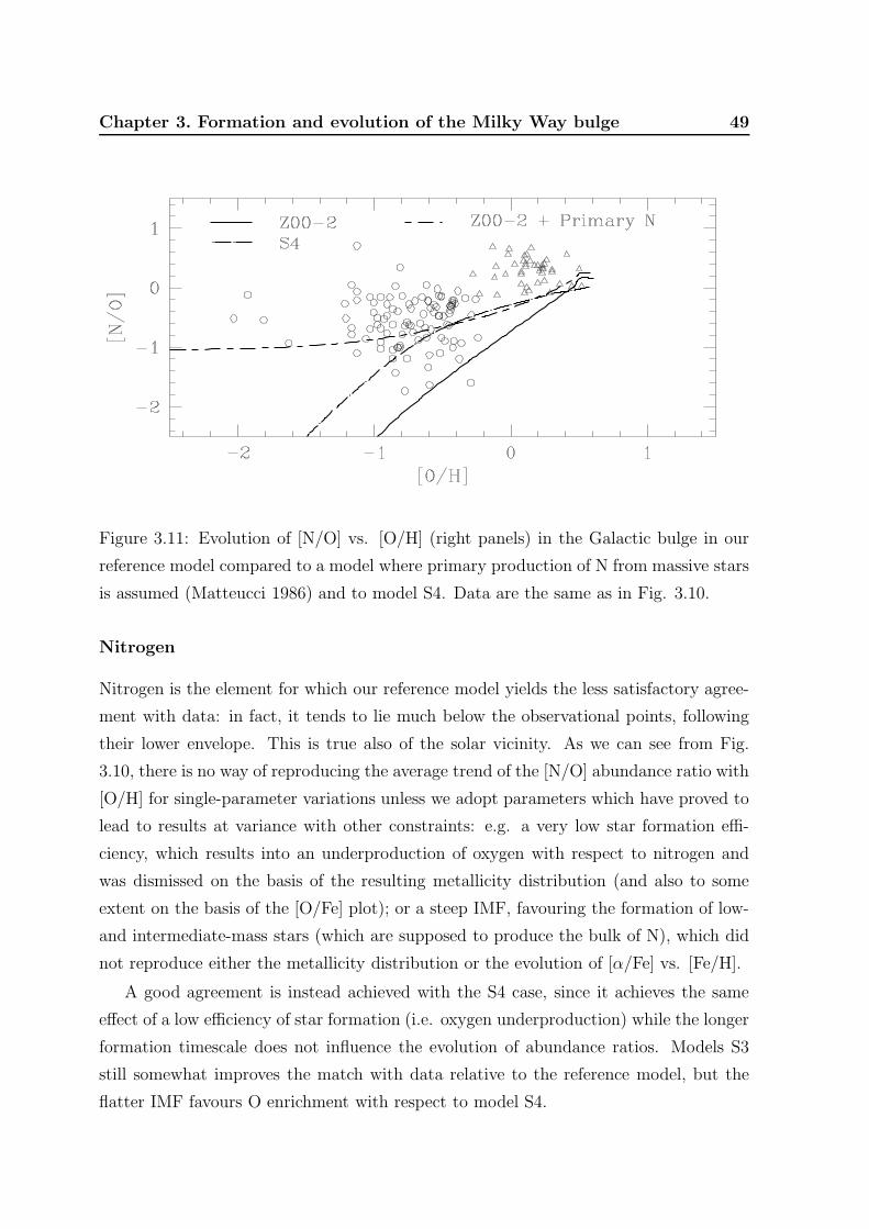
Chapter 3. Formation and evolution of the Milky Way bulge 49
Figure 3.11: Evolution of [N/O] vs. [O/H] (right panels) in the Galactic bulge in our
reference model compared to a model where primary production of N from massive stars
is assumed (Matteucci 1986) and to model S4. Data are the same as in Fig. 3.10.
Nitrogen
Nitrogen is the element for which our reference model yields the less satisfactory agree-
ment with data: in fact, it tends to lie much below the observational points, following
their lower envelope. This is true also of the solar vicinity. As we can see from Fig.
3.10, there is no way of reproducing the average trend of the [N/O] abundance ratio with
[O/H] for single-parameter variations unless we adopt parameters which have proved to
lead to results at variance with other constraints: e.g. a very low star formation effi-
ciency, which results into an underproduction of oxygen with respect to nitrogen and
was dismissed on the basis of the resulting metallicity distribution (and also to some
extent on the basis of the [O/Fe] plot); or a steep IMF, favouring the formation of low-
and intermediate-mass stars (which are supposed to produce the bulk of N), which did
not reproduce either the metallicity distribution or the evolution of [α/Fe] vs. [Fe/H].
A good agreement is instead achieved with the S4 case, since it achieves the same
effect of a low efficiency of star formation (i.e. oxygen underproduction) while the longer
formation timescale does not influence the evolution of abundance ratios. Models S3
still somewhat improves the match with data relative to the reference model, but the
flatter IMF favours O enrichment with respect to model S4.

50 3.3 Results
However, there is another way to obtain an acceptable fit to the observed abun-
dances. In standard chemical evolution models nitrogen production from massive stars
is supposed to be purely secondary, i.e. N is created starting from seed nuclei of C
already present in the gas out of which the stars were born. Also low- and intermediate-
mass stars are supposed to produce N in a secondary fashion but some primary N can be
produced in intermediate mass stars during the third dredge-up episodes in conjunction
with hot-bottom burning3 (Renzini & Voli 1981; Van den Hoek & Groenewegen 1997).
The consequence of the secondary production is that the abundance of nitrogen should
increase with metallicity in the earliest evolutionary phases, and that is what most evo-
lutionary models of the Galaxy predict, not only for the bulge, but also for the solar
neighbourhood (Ballero et al. 2006; Chiappini et al. 2005).
Therefore, we investigate what happens to the reference model if we assume that
massive stars of all masses produce a constant amount (0.065M) of primary N at
every metallicity. This hypothesis follows from the heuristic model of Matteucci (1986).
The results are shown in Fig. 3.11 together with the plot of model S4. We see that this
model seems to reproduce the average trend of the observations better than the standard
model and, although it adopts an ad hoc assumption, it is useful to understand that
some mechanism of primary production of nitrogen is likely to occur at any metallicity
in massive stars. For example, Meynet & Maeder (2002) calculated that stellar rotation
can produce primary nitrogen in massive stars, and although Chiappini et al. (2003b)
demonstrated that their rotation yields are insufficient to produce the observed trend
in the solar neighbourhood, this hypothesis is the most promising one, as shown by
Chiappini et al. (2006). We thus suggest that a continuous primary N production from
massive stars is necessary at any epoch, in analogy with what is required in the solar
vicinity (see Chiappini et al. 2005, for an extensive discussion on this point).
From Fig. 3.10 one can also notice that model S4 differs from model Z00-2 with
primary N for [O/H] . −1, since while in the latter the [N/O] ratio is almost independent
of [O/H], in the S4 model the plot curves down sharply at low metallicities due to
secondary production from massive stars, and at [O/H] ∼ −1 primary production from
low- and intermediate-mass stars becomes dominant.
A certain amount of self-pollution is required in any case to reproduce the [N/O]
ratios measured in giants for [O/H] & 0.
3The penetration of the convective envelope into the hydrogen burning shell, which leads to nucle-
osynthetic processes at the base of the envelope.

Chapter 3. Formation and evolution of the Milky Way bulge 51
3.4 Summary and conclusions
We have tested our new chemical evolution models for the Galactic bulge against new
observations, unavailable at the time of earlier chemical evolution models (e.g., Mat-
teucci & Brocato 1990; Renzini 1993; Matteucci, Romano & Molaro 1999; Molla et
al. 2000). We have considered a scenario involving evolutionary timescales much faster
than in the solar neighbourhood and in the halo as the most probable one. We have
also adopted new chemical yields suggested by Francois et al. (2004) which provided
the best fit to the solar neighbourhood abundance trends in the model of Chiappini et
al. (2003b).
The agreement between the new observations and our predictions is quite good,
especially for the Fe abundance distribution and the [α/Fe] trends.
Order-of-magnitude changes in the main parameters determining chemical evolution
(star formation efficiency, stellar IMF, timescale of gas collapse) were applied in order to
explore the consequences of such changes on the predicted stellar metallicity distribution
and trend of chemical abundances as a function of metallicity.
Our main conclusions can be summarised as follows:
- A short formation timescale combined with a high star formation efficiency fits
both the observed metallicity distribution and chemical abundance ratios. This is
typical of a star formation history in a burst regime, i.e. strongly concentrated in
the first stages of the lifetime of the system and vanishing very quickly, in analogy
with elliptical galaxies. We suggest an efficiency of star formation of the order of
20 Gyr−1. However the assumption of a closed box must be given up since it gives
rise to an excessive amount of low-metallicity stars (even though not as seriously
as in the case of the G-dwarf problem for the solar neighbourhood). A finite,
though small, accretion time is instead required. We suggest that this timescale
should be of the order of 0.1 Gyr.
- There exists a sort of degeneracy between the gas infall timescale and the efficiency
of star formation, in the sense that values of τ longer than 0.1 Gyr can combine
with values of ν lower than 20 Gyr−1 in order to match the observed metallicity
distribution. However, such a degeneracy is broken when we consider also the
evolution of [O/Fe] vs. [Fe/H] and in any case values of τ longer than 1 Gyr do
not allow to fit the observed metallicity distribution as well.

52 3.4 Summary and conclusions
- An IMF flatter than those suitable for the solar neighbourhood properties, such
as that of Scalo (1986) or Weidner & Kroupa (2005), is necessary to reproduce
the observational constraints. Namely, a value of x = 0.95 for massive stars
(even smaller than that proposed by Matteucci et al. 1999, which was x = 1.1)
gave the best overall fit. This can be theoretically understood if we note that
the star formation in the bulge proceeds like in a burst and there are several
suggestions in the literature about a top-heavy IMF in starbursts (e.g. Baugh et
al. 2005, Nagashima et al. 2005). Figer (2005) also finds a flat IMF in the Arches
cluster near the Galactic centre. The adopted flattening below 1M (x = 0.33),
as suggested by luminosity function measurements (Zoccali et al. 2000) does not
affect significantly the abundance distribution. However, extremely flat IMFs (e.g.
that of Z00-1 model), if extrapolated to massive stars, will lead to some degree of
oxygen overproduction.
- The adoption of the reference model explains the behaviour of the different [α/Fe]
abundance ratios with metallicity very well, and predicts different slopes for dif-
ferent α-elements, according to their nucleosynthesis. There is no need to invoke
a second infall episode, as suggested by other authors (Molla et al. 2000; Costa
et al. 2005) to explain the observed values of the abundance ratios. We do not
exclude however a second infall episode on a much longer timescale such as that
hypothesised by Molla et al. (2000) as it may help explain the presence of a very
young stellar population confined to the very centre of our Galaxy (e.g. Groe-
newegen & Blommaert 2005), but it must involve a minor fraction of the bulge
gas mass.
- A certain amount of primary nitrogen from massive stars might be required in
order to reproduce the average trend of [N/O] vs. [O/H] with the reference model.
The same conclusion was reached for the solar neighbourhood by Chiappini et
al. (2005) and Ballero et al. (2006). The phenomenon of primary N production
from massive stars as a result of rotation was studied by Meynet & Maeder (2002,
2003, 2005) and Hirschi (2007) and although their yields are still not sufficient to
explain the observed trend, this seems the most promising way (see Chiappini et al.
2006). These considerations followed from observations of N and O abundances in
planetary nebulae; in order to firmly assess this point, abundance measurements in
stars which have not experienced nitrogen self-enrichment are required, especially

Chapter 3. Formation and evolution of the Milky Way bulge 53
at low metallicities. In alternative, carbon measurements in the same planetary
nebulae we have considered might allow an estimate of the amount of N synthesised
by the planetary nebula progenitor.
- In the near future new sets of empirical metallicity and abundance pattern dis-
tributions in different fields and based on high-resolution spectroscopy will also
become available. This will dramatically improve the chance of a more robust and
quantitative comparison between theory and observations, with the ultimate goal
of drawing the formation and chemical evolution history of the Galactic bulge.

54 3.4 Summary and conclusions

Chapter 4
O and Mg evolution in the Galactic
bulge and solar neighbourhood
4.1 Mass loss and stellar yields
Mass loss in massive stars occurs due to the interaction of radiation flowing through
the atmosphere of a star and the matter in the atmosphere. In massive stars, radiation
pressure is important and their luminosity is a non-negligible fraction of the star’s Ed-
dington luminosity1, i.e. the luminosity at which the radiation pressure overwhelms the
gas pressure in the atmosphere, and which is given by:
LEdd,∗ =4πcGMenv
ks
(4.1)
where Menv is the envelope mass and ks is the stellar surface opacity. The ionised
atoms in the atmosphere absorb radiation and a net movement outwards is achieved;
the absorbers are mainly metals. In the so-called Wolf-Rayet stars, with masses above
25−30M, mass loss rates can reach MWR ' 10−4M/yr. This way, they can lose their
hydrogen envelope and explode as Type Ib supernovae (core-collapse supernovae with
no H in their spectra), or even lose the helium envelope, in which case they explode as
Type Ic supernovae (which miss He as well in their spectra).
Stellar yields can be affected by mass loss in massive stars. Maeder (1992) computed
the wind contributions in He, C, N, O and Ne in stars in the mass range 1 − 120M
and for metallicities Z = 0.001 and Z = 0.02. He found that, at solar metallicities and
1The reader must not confuse the stellar Eddington luminosity mentioned here with the Eddington
luminosity defined for black holes in §6.5.2.

56 4.1 Mass loss and stellar yields
above, large amounts of He and C are ejected into the interstellar medium, reducing the
synthesis of heavier elements; thus C and He are produced at the expense of O, while the
same effect is not seen at low metallicities. Therefore, the nucleosynthesis production
strongly depends on the initial stellar metallicity. The metallicity dependence of the
stellar wind is due to the opacity of the material in the radiation-driven mass loss of
massive stars, as originally proposed by Lucy & Solomon (1970). The effect of mass
loss on stellar yields as a function of metallicity is particularly strong for Wolf-Rayet
stars. By means of these stellar models Maeder (1992) was able to reproduce the number
statistics of Wolf-Rayet and O-type stars in nearby galaxies with various metallicities.
Later, Langer & Henkel (1995) also computed He and CNO isotope yields for mass-
losing stars in the range 15 ≤M/M ≤ 50. They also found drastic differences relative
to models without mass loss for the yields of oxygen in metal-rich stars more massive
than 30M.
More recently, Meynet & Maeder (2002, 2003, 2005) and Hirschi (2007) have com-
puted a grid of models for stars with masses > 20M, including rotation and metallicity-
dependent mass loss. The effect of metallicity-dependent mass loss in decreasing the O
production in massive stars was confirmed, although they employed significantly lower
mass loss rates, based on work by Vink et al. (2000) and Nugis & Lamers (2000). The
new and improved mass-loss rates are factors of 2 to 3 lower than previously adopted
by Maeder (1992); however, with these mass-loss rates and the inclusion of rotation the
models are able to reproduce the frequency of Wolf-Rayet and O stars, the observed
WN/WC ratio2, and the observed ratio of Type Ib/Type Ic supernovae at different
metallicities. It appears that the earlier high mass-loss rates made up for the omission
of rotation in the stellar models. In galactic chemical evolution models, the effect of
the Maeder (1992) yields was studied by Prantzos, Aubert & Audouze (1996), who con-
cluded that the mass loss in massive stars has strong effects on the production of C and
O.
In summary, the effect of metallicity-dependent mass loss on stellar yields appears
relevant for stars with solar metallicities or larger, and therefore it should be taken
into account in computing the bulge chemical evolution and the late stages of chemical
evolution in the solar vicinity.
2Wolf-Rayet stars are subdivided into three subgroups according to their spectral features. Among
these subgroups, WN are Wolf-Rayet stars where N dominates over C in their spectra, and WC are
those where C dominates instead. The rare WO stars have C/O < 1.

Chapter 4. O and Mg evolution in the bulge and solar neighbourhood 57
4.2 Evidence for metallicity-dependent O yields
Oxygen and magnesium are among the most easily understood elements because their
synthesis is restricted to well known processes in the cores of massive stars and they are
thought to be unaffected by the complications of explosive nucleosynthesis (e.g. Woosley
& Weaver 1995). They are particularly interesting as probes of massive stars and the
SFR in chemically evolving stellar systems. Thus, one might expect that O and Mg
abundances should vary in lock-step in all, or most situations, since O and Mg are both
thought to be produced only by stars that end as core-collapse supernovae.
However, McWilliam & Rich (2004) found a steeply declining [O/Fe] ratio in the
bulge stars with a slope almost consistent with no production of O above [Fe/H] & −0.5.
They suggested an O yield decline due to winds from massive stars, related to the Wolf-
Rayet phenomenon. Later Fulbright et al. (2007) noted the apparent discord between
nearly flat, enhanced, [Mg/Fe] and yet declining, although enhanced [O/Fe] in the bulge
above [Fe/H] ∼ −1.0; again, they suggested declining metallicity-dependent O yields
related to the Wolf-Rayet phenomenon. Lecureur et al. (2007) also found a decreasing
trend for [O/Mg] in the bulge stars, and suggested a difference in the stellar yields of O
and Mg from massive stars.
This observed difference between Mg and O trends could potentially lead to a conflict
in the estimated SFR and formation timescale of the bulge: if the steeper decline of
[O/Fe], compared to [Mg/Fe], with increasing metallicity is due to the addition of Fe
from Type Ia supernovae, then a lower SFR and longer bulge formation timescale would
be indicated from O than for Mg. If the different decline rates for O and Mg are due
to the supernova yields it is necessary to understand them in a consistent picture of
nucleosynthesis and chemical evolution. Because O and Mg are produced only in the
hydrostatic cores of massive stars, then if the O/Mg yield ratio declines as a function
of metallicity, the same trend should be present in stellar systems, no matter what
the SFR, provided that the formation timescale is long enough to permit all masses of
Type II supernovae to occur. In fact, different slopes in the [Mg/Fe] and [O/Fe] ratios
are visible in metal rich stars in the solar vicinity, where the [Mg/Fe] seems to reach a
plateau for [Fe/H] > 0, but the [O/Fe] ratio continues to decrease (see Edvardsson et al.
1993; Castro et al. 1997; Feltzing & Gustafsson 1998; Bensby et al. 2005). This trend
also suggests the effect of strongly metal dependent O yields in metal rich massive stars.
To test the metallicity dependence of the O/Mg ratio we compared (McWilliam et
al. 2008) the abundance ratio of O/Mg seen in the Galactic bulge and in the Galactic

58 4.2 Evidence for metallicity-dependent O yields
thin and thick disks. In particular we use [Mg/H] and [O/H] as metallicity indicators,
rather than [Fe/H], in order to eliminate the effect of Fe from Type Ia supernovae. The
observational evidence for a decrease in the oxygen yield, relative to magnesium, from
Type II supernovae with increasing metallicity is summarised in Fig. 4.1. In the upper
panel of Fig. 4.1 we show a plot of the [O/Mg] versus [Mg/H] for the bulge from the
IR spectroscopic database (defined in Chapter 3), Zoccali et al. (2006), Fulbright et al.
(2007), and Lecureur et al. (2007), compared with points for the solar neighbourhood
thin and thick disks from Bensby et al. (2005). Contrary to what one might expect for
two α-elements produced by the same stars the [O/Mg] ratio is not flat, but declines
steeply for [Mg/H] values larger than −0.5 dex. The same effect is visible both in
the bulge and disk stars. Note that in the lower panel of Fig. 4.1 we show the same
observed [O/Mg] ratio, but with [O/H] as the metallicity indicator. For the bulge
metallicity points we employ the mean [O/H], based on [Fe/H] and a fit to the trend of
[O/H] versus [Fe/H]; it was motivated to reduce the scatter in the [O/H] metallicity axis
resulting from the use of only the 6300 A [O i] line for the oxygen abundances. Oxygen
is useful as a metallicity indicator, despite the noise, because it contributes more than
half of the total metallicity, Z. We avoided using the recent oxygen abundances for
thick disk stars by Reddy et al. (2006), because these were based on the high excitation
O i triplet lines near 7771 A, and not on the robust [O i] 6300 A indicator; the high
excitation O i lines require uncertain corrections for non-LTE3 effects.
In both figures there is a clear decline in the bulge [O/Mg] ratio of ∼ 0.8 dex from
low to high metallicity, including a markedly steeper descent above solar metallicity.
It is notable, and very important, that the [O/Mg] trends for the Galactic disk closely
overlap the bulge trends, and that both show the steeper decline above solar metallicity.
A similarity in the evolution of the products of Type II supernovae in the disk and
bulge is expected because O and Mg are produced on the same timescales. On the
other hand, we expect to see the effect of the time delay model in the [α/Fe] ratios.
We suggest that, to within the measurement uncertainties, the disk and bulge [O/Mg]
versus [Mg/H] trends are the same. However, there is some leeway in this interpretation
with a possibility that the bulge [O/Mg] ratios slightly exceed the disk ones for a given
[Mg/H]. Some of the individual bulge studies may show offsets from the disk trend,
but these are small; in this regard we note that in the Fulbright et al. (2007) study
there was some evidence to support a systematic downward zero-point correction to the
3Local Thermodynamic Equilibrium.

Chapter 4. O and Mg evolution in the bulge and solar neighbourhood 59
oxygen abundances, by ∼ 0.04 dex; if applied this would make a slight improvement to
the already good agreement between disk and bulge O/Mg relations.
Fig. 4.1 also compares the composition of the bulge, formed within the initial ∼1 Gyr
after the Big Bang, with the composition of disk stars formed up to the present epoch.
The trend with [Mg/H] as metallicity indicator is particularly important because the
[Mg/Fe] ratios in the bulge are significantly higher than in the disk due to Fe from
Type Ia supernovae. Given these differences between the disk and bulge it is remarkable
that the [O/Mg] trends with [Mg/H] and [O/H] follow each other so closely.
We begin to understand the O/Mg ratio trend by appreciating that both O and Mg
are thought to be produced only by core-collapse supernovae. In particular it should
be remembered that O production increases strongly with pre-supernova mass (e.g.
Woosley & Weaver 1995), but more important for this investigation is the trend of
O/Mg yield ratio with supernova progenitor mass. The Francois et al. (2004) yields
show a strongly increasing O/Mg ratio with mass, with a range exceeding 1.5 dex. This
high sensitivity to progenitor mass is similar to the predictions for hypernovae computed
by Fryer et al. (2006); however, results from other calculations (Woosley & Weaver 1995,
Tsujimoto et al. 1995, Nomoto et al. 1997, Limongi & Chieffi 2003, Kobayashi et al.
2006) show very shallow O/Mg trends with mass. A steeper O/Mg yield ratio with mass
is due to Arnett (1991), with a range of ∼ 0.5 dex.
If the O/Mg yield ratio is strongly sensitive to the mixture of supernova masses, the
observed abundance ratios will be affected by the IMF. In particular, a flatter bulge
IMF than the galactic disk would produce a higher [O/Mg] ratio in the bulge, if other
parameters remain the same. However, the data seems to show a large overlapping of the
[O/Mg] ratio in the bulge and disk stars, although some bulge stars show a higher ratio.
In the previous Chapter, a flat IMF for the bulge was suggested in line with previous
results (e.g. Matteucci & Brocato 1990, Matteucci et al. 1999), based on the observed
bulge stellar metallicity distribution, which cannot be reproduced with the same IMF as
the disk with the current set of parameters (this topic will be discussed more extensively
in the next Chapter). Thus, the similarity of the O/Mg ratios in the bulge and disk
suggests that either the O/Mg yield ratio is quite insensitive to stellar mass, in which
case the yields of Francois et al. (2004) need to be modified, or that the IMF for the
bulge is similar to that of the disk, with much less of a difference in slope than indicated
in Chapter 3. More data will help to decide whether the abundance ratios in the bulge
are higher or equal to those in the solar vicinity, while further theoretical and empirical

60 4.2 Evidence for metallicity-dependent O yields
Figure 4.1: Data for the bulge (filled circles, plus signs and open triangles; see Fig 3.2 for
references) compared with solar vicinity stars (crosses, Bensby et al. 2005) for [O/Mg]
vs. [Mg/H] (upper panel) and [O/Mg] vs. [O/H] (lower panel).

Chapter 4. O and Mg evolution in the bulge and solar neighbourhood 61
studies may constrain the O and Mg yields from massive stars.
If O/Mg yields are a function of stellar mass the observed downward slope in [O/Mg]
vs. [Mg/H] could be explained by a metallicity-dependent IMF, that increases the
fraction of low-mass supernovae at higher metallicity; this would apply to both the disk
and the bulge, but there is no evidence of a variable IMF in the disk. Therefore, we
discard the notion of a metallicity-dependent IMF to explain the observed O/Mg trend.
Supposing that the O/Mg yields increase strongly with stellar mass, then during
initial enrichment O/Mg ratios would be higher than at later times, because massive
stars are the first to end as supernovae. Thus, over the period spanning the lifetime of
massive stars there should be a decline in the average O/Mg ratio of a system. This low-
metallicity effect might be seen at a higher metallicity in the bulge than other Galactic
locations, due to the high SFR in the bulge. We adopt the simple notion that the
observed similarity of the O/Mg slopes for both the Galactic disk and bulge reflects
a metallicity modulation of the yields from core collapse supernovae; in principle this
could be due to O or Mg yields, or both.
The bulge results are similar to those of Bensby et al. (2004), who identified the
decline in [O/Mg] versus [Mg/H] in the Galactic thin and thick disk populations. They
considered the possibility that metallicity-dependent O yields from massive stars could
explain the observed trend, but dismissed this idea based on their interpretation of
the O yields of massive stars from models, including rotation, by Meynet & Maeder
(2002). Our understanding is that while rotation does increase the core mass, the effect
of decreased O yields with increasing metallicity, due to mass loss, is clear in the works
of Meynet & Maeder (2002, 2003, 2005) and Hirschi (2007); the effect on the yields
is particularly noticeable for the most massive stars above solar metallicity (Meynet &
Maeder 2005, Hirschi 2007). This result holds, despite the decrease in adopted mass-loss
rates, compared to Maeder (1992).
4.3 The chemical evolution models
While for the Galactic bulge we made use of the model described in Chapters 2 and 3,
for the chemical evolution of the Milky Way disk we adopted the model of Chiappini
et al. (1997) with updated nucleosynthesis prescriptions as in Francois et al. (2004).
This model is the so-called two-infall model where the halo and part of thick disk are
formed during a first relatively short episode (< 2 Gyr) of accretion and star formation,

62 4.4 Results
whereas the thin disk formed out of a second independent infall episode which lasted
much longer (∼ 8 Gyr in the solar vicinity) and formed the disk “inside-out”. The
adopted IMF is the one from Scalo (1986) and is considered constant in space and time;
the star formation efficiency is ν = 1 Gyr−1.
In order to investigate the potential effect of mass loss on predicted O/Mg ratios
we decided to update our current model with the Maeder (1992) yields that take into
account the effect of mass loss for massive stars as a function of metallicity. We used the
Maeder (1992) yields, rather than the latest results of Meynet & Maeder (2005), in order
to maintain consistency with the pre-existing model employing the Woosley & Weaver
(1995) yields; both Woosley & Weaver (1995) and Maeder (1992) models ignore the
effects of rotation, but both provide similar yields near solar metallicity. In this way our
calculation should show how the metallicity-dependent yields affect the current model.
In Fig. 4.2 we can see the differences between the yields of oxygen of Woosley &
Weaver (1995) and Maeder (1992) for two different initial stellar metallicities. The effect
of the metallicity-dependent mass loss is evident in the figure: especially for stars with
masses larger than 25M and solar metallicity the O production is strongly depressed
due to mass loss.
4.4 Results
4.4.1 [O/Mg] vs. [O,Mg/H]
In Fig. 4.3 we show the same data as in Fig. 4.1, but the theoretical predictions for
the bulge and disk are superimposed. As one can see in both cases the slope of the
[O/Mg] ratio is very well reproduced by the Maeder (1992) yields. In particular, both
the observations and our predictions indicate a sudden steepening of the slope above
solar metallicity, with good agreement between the predicted and observed slopes below
and above the break-point.
In the present chapter, our model results have been normalised to the solar abun-
dances predicted by the Milky Way model, which gives a very good fit to the Asplund et
al (2005) solar abundances. The ∼0.2 dex zero-point offset between our predicted bulge
[O/Mg] trend and the data suggests that either the yields of Francois et al. (2004) re-
quire adjustment, or that the adopted IMF of our reference model (Ballero et al. 2007a)
is too flat, or a combination of these effects. Normalisation of the predictions to solar
abundances is also an issue.

Chapter 4. O and Mg evolution in the bulge and solar neighbourhood 63
Figure 4.2: Comparison between the O yields of Maeder (1992) and Woosley & Weaver
(1995) for massive stars as functions of initial stellar mass. The dramatic decline of O
yields from high mass stars at solar metallicity for the Maeder (1992) models is due to
mass loss of the outer layers, which prevents He and C from being synthesised into O.
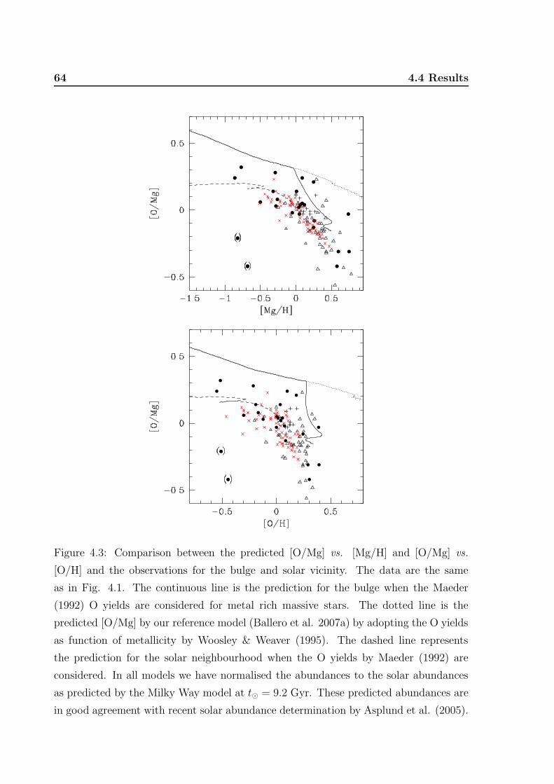
64 4.4 Results
Figure 4.3: Comparison between the predicted [O/Mg] vs. [Mg/H] and [O/Mg] vs.
[O/H] and the observations for the bulge and solar vicinity. The data are the same
as in Fig. 4.1. The continuous line is the prediction for the bulge when the Maeder
(1992) O yields are considered for metal rich massive stars. The dotted line is the
predicted [O/Mg] by our reference model (Ballero et al. 2007a) by adopting the O yields
as function of metallicity by Woosley & Weaver (1995). The dashed line represents
the prediction for the solar neighbourhood when the O yields by Maeder (1992) are
considered. In all models we have normalised the abundances to the solar abundances
as predicted by the Milky Way model at t = 9.2 Gyr. These predicted abundances are
in good agreement with recent solar abundance determination by Asplund et al. (2005).

Chapter 4. O and Mg evolution in the bulge and solar neighbourhood 65
Given that the bulge metallicity function suggests a flatter IMF than the disk (Ballero
et al. 2007b; see next Chapter) and the difficulties involved with inverting chemical
evolution models to obtain element yields, we suspect that the problem most likely
arises in the adopted O/Mg yields of Francois et al. (2004). As we noted earlier the
O/Mg yield trend with supernova progenitor mass, suggested by the results of Francois
et al. (2004), is much steeper than most theoretical predictions; if this steep slope is in
error we would expect to see an artificial zero-point offset in the predicted O/Mg ratio.
The zero-point problem does not concern the main conclusion that diminished oxygen
yields, due to mass-loss from high metallicity Type II supernovae are responsible for the
observed declining [O/Mg] trend with increasing [Mg/H] in the Galactic bulge and disk.
This resolves the apparent discord between the bulge trends of [Mg/Fe] and [O/Fe] with
[Fe/H]; now both are consistent with a high SFR in the bulge.
It is worth recalling that Asplund et al. (2005) found a lower O abundance in the
sun than Grevesse & Sauval (1998), whereas there is little difference for the abundances
of Mg and Fe. In Fig. 4.4 we show the same plot as in Fig. 4.3, but only for the
bulge; the agreement between the slope predicted with Maeder (1992) yields and the
data is again very good. Again, the predicted absolute values are higher than the data,
but this depends on the normalisation to the solar abundances. In our reference model,
where the solar abundances were those of Grevesse & Sauval (1998), the predicted
[O/Mg] was lower, due to the higher O solar abundance suggested by Grevesse & Sauval
(1998) relative to Asplund et al. (2005). In Fig. 4.4 we also show the same model
predictions normalised to the Grevesse & Sauval (1998) solar abundances. We stress
that the important points are that the slopes and break-points in the [O/Mg] trends
with metallicity. It is also important to note that the predicted [O/Mg] in the bulge
is higher than in the solar neighbourhood. In our models this mainly depends on the
assumed IMF in the bulge which is flatter than in the solar vicinity. Such a flatter
IMF seems to be unavoidable in order to reproduce the observed stellar metallicity
distribution in the bulge, as extensively discussed in the next Chapter. The bulge
parameters of our reference model concerning the IMF, SFR and infall timescale are not
affected by the consideration of mass-loss dependent yields investigated here. For the
IMF and SFR the work discussed in Chapter 3 was entirely constrained by [O/Fe] at
metallicities below solar, for which mass-loss dependent yields are not a factor. While
the [O/Fe] predictions of Chapter 3 provided a slightly better fit with in infall timescale
near 0.7 Gyr, the metallicity distribution function excluded such value. In any case, the

66 4.4 Results
Figure 4.4: Predicted and observed [O/Mg] vs. [Mg/H] only for the bulge. The model
(continuous line) is the one with Maeder’s (1992) yields. The upper line refers to the
predicted bulge abundances normalised to the solar predicted values by the Milky Way
disk model, as in the curves of Fig. 4.3. The lower line instead refers to the predicted
bulge abundances normalised to the Grevesse & Sauval (1998) solar abundances. The
offset between the two curves mainly results from the solar abundances predicted by our
model, which is in very good agreement with the one suggested by Asplund et al. (2005),
but lower than previous estimates. Data sources: plus signs are the IR spectroscopic
database (see §3.2 for specific references); open triangles are the data of Zoccali et al.
(2006) and Lecureur et al. (2007); filled circles are the data from Fulbright et al. (2007).

Chapter 4. O and Mg evolution in the bulge and solar neighbourhood 67
metallicity-dependent oxygen yields considered here are consistent with τ = 0.1 Gyr,
which is the value adopted in our reference model.
4.4.2 [O/Fe] vs. [Fe/H]
The [O/Mg] vs. [Mg/H] or [O/Mg] vs. [O/H] plots do not contain the effects produced
by the chemical enrichment of Type Ia supernovae, but only depend on the different
yields for O and Mg because these two elements are produced on similar timescales. On
the other hand, the effect of Type Ia supernova enrichment is clearly visible in the [α/Fe]
vs. [Fe/H] plots, where the change in slope of the [O,Mg/Fe] ratios is mainly due to the
time-delay with which the bulk of Fe is injected into the interstellar medium by Type Ia
supernovae. The history of star formation plays an important role in the [α/Fe] versus
[Fe/H] diagrams: in the bulge, which is assumed to have suffered an intense, burst-like
star formation we expect a long plateau of enhanced α’s and a turning point occurring
at [Fe/H] ≥ 0, as opposed to the disk where the star formation proceeded much more
smoothly and therefore we expect the turning point to occur at lower metallicities; and
even more so in dwarf galaxies (Lanfranchi & Matteucci, 2004) where the star formation
proceeded extremely slowly, thus giving rise to low [α/Fe] ratios at low [Fe/H]. The
predictions for [O/Fe] versus [Fe/H] in the bulge compared with data can be seen in
Fig. 4.5, and the fit is again excellent, also in the absolute value. The [O/Fe] predicted
by our reference model (Ballero et al. 2007a) at high metallicities was flatter and in less
good agreement with the observed points.
The metallicity-dependent decline in the oxygen yield brings understanding to the
long-standing apparent discrepancy between the trend of [O/Fe] at high [Fe/H] and
the [α/Fe] trends for Mg, Si, Ca and Ti in the Galactic disk. In the standard time-
delay explanation for the decline of [α/Fe] with [Fe/H] all these elements should show
similar declines. However, in the Galactic disk [O/Fe] continues a roughly linear decline
above solar [Fe/H] to negative [O/Fe] values (Edvardsson et al. 1993, Castro et al.
1997, Feltzing & Gustafsson 1998, Bensby et al. 2004). The other α-elements reach
a low plateau in [α/Fe], at the solar ratio, beginning near [Fe/H] ∼ −0.4 to −0.2 dex;
and this plateau continues to the most metal-rich disk stars. The unusual behaviour of
oxygen is unexpected from the pure time-delay explanation for the decline in [α/Fe] with
increasing [Fe/H] in the Galactic disk; however, the time-delay model well describes the
plateau seen in the other α-elements, the α-enhancements seen in bulge stars (McWilliam
& Rich 1994; Fulbright et al. 2007), subsolar [α/Fe] ratios seen in small subgroups of
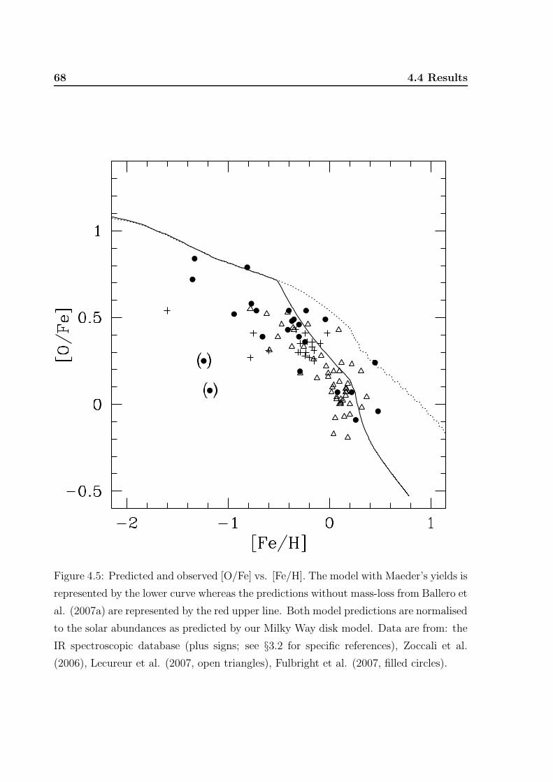
68 4.4 Results
Figure 4.5: Predicted and observed [O/Fe] vs. [Fe/H]. The model with Maeder’s yields is
represented by the lower curve whereas the predictions without mass-loss from Ballero et
al. (2007a) are represented by the red upper line. Both model predictions are normalised
to the solar abundances as predicted by our Milky Way disk model. Data are from: the
IR spectroscopic database (plus signs; see §3.2 for specific references), Zoccali et al.
(2006), Lecureur et al. (2007, open triangles), Fulbright et al. (2007, filled circles).

Chapter 4. O and Mg evolution in the bulge and solar neighbourhood 69
halo stars (Brown et al. 1997; Nissen & Schuster 1997) and the decline in [α/Fe] ratios
at lower [Fe/H] in dwarf galaxies (Geisler et al. 2005).
The solution is that in the disk both the time delay reduction in [α/Fe] and metallicity-
dependent decline in oxygen yields operate; this is why the [O/Fe] ratios show a different
behaviour than other α-elements in super-metal-rich stars.
4.5 Summary and conclusions
A summary of recent observational measurements of [O/Mg] versus [Mg/H] and [O/H]
indicate that the [O/Mg] ratio have similar trends in the Galactic bulge and solar neigh-
bourhood.
We reject the possibility that a metallicity-dependent IMF in the disk and bulge is
responsible for the observed slopes. The similarity of abundance trends for the two sys-
tems suggests a metallicity-dependent modulation of the supernova O/Mg yield ratio.
The O/Mg slope is qualitatively consistent with a metallicity-dependent decline in oxy-
gen yields due to winds from massive stars, and related to the Wolf-Rayet phenomenon,
as suggested by McWilliam & Rich (2004) and Fulbright et al. (2007).
To quantitatively test the significance of metallicity-dependent mass loss from mas-
sive stars on the O/Mg trend in the bulge and disk we have extended the bulge chemical
evolution model of Ballero et al. (2007a) discussed in the previous Chapters by including
the metallicity-dependent oxygen yields of Maeder (1992) resulting from stellar winds
in massive stars. We find that the predicted slopes and break-points of the [O/Mg]
trend with [O/H] and [Mg/H], and [O/Fe] versus [Fe/H], are very well reproduced with
the inclusion of mass loss, although zero-point differences of up to ∼0.2 dex exist with
observations. The inclusion of the metal-dependent O yields into the Ballero et al.
(2007a) model substantially improves the comparison between observed and predicted
abundance trends. Thus, the simple inclusion of the known effects of mass-loss on the
oxygen yields of massive stars is enough to explain much of the O/Mg trend in the bulge
and disk.
The ∼0.2 dex zero-point difference between our calculations and the observations
indicates that either the semi-empirical yields of Francois et al. (2004) have too high
a sensitivity on supernova progenitor mass, or that the IMF of our reference model is
too flat; the observations might also be explained with a combined change of yields and
IMF. Future observations and theoretical investigations into yields from massive stars

70 4.5 Summary and conclusions
are required to resolve this issue. However, preliminary calculations indicate that by
adopting Salpeter (1955) IMF, although it reduces the offset in the [O/Mg] plots, the
correct slope and break point for supersolar metallicities are poorly reproduced. On the
other hand, a plot obtained with a model where a Scalo (1986) IMF is adopted does not
cover the whole range of [Mg/H] values but only extends up to ∼solar [Mg/H].
By including the Maeder (1992) metal-dependent yields we remove the previous
disagreement between the IMF slope obtained by the fit of the model illustrated in the
previous Chapter to the trend of [O/Fe] with [Fe/H] compared to the slope we found
by fitting the metallicity distribution function. Now the methods give consistent results
for the IMF slope.
Our improvement to the chemical evolution predictions concerning the O/Mg slope
greatly reduces the apparent inconsistency between [O/Fe] and [Mg/Fe] trends in the
high metallicity bulge stars: both elements are more consistent with a rapid bulge
formation timescale, as suggested by Matteucci et al. (1999) and Ballero et al. (2007a).

Chapter 5
Universal or
environment-dependent IMF?
5.1 The issue of the IMF
The question of which is the most suitable initial mass distribution for bulges of galaxies
is not addressed very often. In fact, bulge evolution models (e.g. Samland et al. 1997;
Ferreras et al. 2003; Immeli et al. 2004; Costa et al. 2005) usually assume a priori
that the zero age main sequence masses of stars are distributed following a power-law
distribution:
φ(m) ∝ m−(1+x) (5.1)
with a Salpeter (1955) index (x = 1.35). Basic physical arguments support the idea of
an IMF varying among different environments (see e.g. Padoan et al. 1997; Larson 1998;
or Nakamura & Umemura 2001; Schaerer 2002; Bromm & Larson 2004 for Population
III stars).
On the other hand, so far there has not been a convincing observational evidence
of such a variation in the stellar IMF based on direct stellar counts (see e.g. Chabrier
2003 for an extensive review). Massey (1998) find that the IMF is well represented by a
Salpeter slope over an order of magnitude in metallicity, in the clusters and associations
of the Milky Way and Magellanic Clouds, as well as in OB associations, while the slope
appears to be much steeper in the field (x ∼ −3). The invariance of the stellar IMF was
confirmed by subsequent works. Kroupa (2001) summarised the available constraints
by means of the multi-part power-law shape
φ(m) ∝ m−(1+xi) (5.2)

72 5.1 The issue of the IMF
where
x1 = 0.3 for 0.08 ≤ m/M ≤ 0.5
x2 = 1.3 for 0.5 ≤ m/M
(5.3)
which we call the Universal IMF (UIMF).1
However, the IMF integrated over galaxies, which controls the distribution of stellar
remnants, number of supernovae, and the chemical enrichment of a galaxy, is generally
different from the stellar IMF and is given by the integral of the latter over the embedded
star-cluster mass function, which varies from galaxy to galaxy. Weidner & Kroupa (2005)
find such integrated galaxial IMF (IGIMF) to be steeper than the UIMF for a range of
plausible scenarios, and they suggest a “maximum scenario”, based on the Scalo (1986)
star-count analysis of the local Galactic field, with an IGIMF which has the following
indexes:
x1 = 0.3 for 0.08 ≤ m/M ≤ 0.5
x2 = 1.3 for 0.5 ≤ m/M ≤ 1
x3 = 1.7 for 1 ≤ m/M
(5.4)
In the following, we will refer to this IMF as to the IGIMF.
Conversely, Piotto & Zoccali (1999) and Paresce & De Marchi (2000) measured the
present-day mass function in Galactic globular clusters below ∼ 0.7M. They found
evidence of variation in the slope of the mass function among different environments,
with a tendency toward flatter slopes in globular clusters compared to the Galactic field
IMF; Paresce & De Marchi (2000) also state that, in the considered mass range, the
observed mass function represents the true stellar IMF for these environments. Zoccali
et al. (2000) derived the IMF below 1M in the Galactic bulge and concluded that it
is shallower than the Salpeter slope; it also shows similarity with the IMF of globular
clusters. However, the somewhat smaller x1 is probably the result of the evaporation
of low-mass stars from the cluster (Baumgardt & Makino 2003), while the Galactic
bulge result is still consistent with the UIMF, within the uncertainties. On the other
hand, Paumard et al. (2006) performed observations of 40 OB supergiants, giants and
main sequence stars in the central parsec of the Galaxy, and concluded that the K-band
luminosity function of massive stars suggests a top-heavy stellar IMF.
Concerning the range of masses over which star formation is possible, although stel-
lar instabilities that potentially lead to disruption already occur above 60 − 120M
(Schwarzschild & Harm 1959), stars of ∼ 140− 155M were observed in the core of the
1This IMF is the form corrected for unresolved binaries.

Chapter 5. Universal or environment-dependent IMF? 73
R136 cluster (Massey & Hunter 1998) and in the Arches cluster (Figer 2005). Although
Massey (2003) sustains that this upper limit may indeed be statistical rather than phys-
ical (i.e. there may not be regions that are rich enough to allow the detection of stars
more massive than that), Oey & Clarke (2005) studied the content of massive stars in
9 clusters and OB associations in the Milky Way and Magellanic Clouds and find that
the expectation value for the maximum stellar mass lies, with high significance, in the
range 120− 200M. This agrees with the conclusion of Weidner & Kroupa (2004) that
a fundamental maximum limit for stellar masses can be constrained at about 150M,
unless the true stellar IMF has x > 1.8.
Attempts to constrain the IMF in the bulge of our Galaxy based on observations of
chemical abundances were carried out by Matteucci & Brocato (1990) and Matteucci
et al. (1999), who fixed the index by the requirement of reproducing the observed
metallicity distributions of Rich (1988) and McWilliam & Rich (1994), respectively.
They both concluded that the bulge IMF must be flatter than the Salpeter one, in
general, and lie in the range x = 1.1 − 1.35, thus favouring the production of massive
stars with respect to the solar vicinity. An even flatter IMF index was chosen in our
investigation (Ballero et al. 2007a), since we showed that it is necessary to assume x2 ' 1
(where x2 is essentially the one defined in Eq. 5.3) to fit the metallicity distributions
of Zoccali et al. (2003) and Fulbright et al. (2006) for the Galactic bulge and of
Sarajedini & Jablonka (2005) for the bulge of M31. Even shallower IMFs (x = 0.33)
are compatible with these observed distributions, but give rise to a certain amount of
oxygen overproduction.
We tested (Ballero et al. 2007b) the effect of adopting both the UIMF and the
IGIMF on the predicted bulge metallicity distribution and to compare the results with
the metallicity distributions employed in Ballero et al. (2007a). These IMFs will be
extended to a much higher upper mass limit than in previous models, so we will try
to find the combination of metal yields and evolutionary parameters that best fit the
observations with these two IMFs.
5.2 Model results
In Chapter 3 we showed that an IMF with the Salpeter (1955) index (x = 1.35) for
1 ≤ m/M ≤ 80 or with the Scalo (1986) index (x = 1.7) for 2 ≤ m/M ≤ 80 could not
fit the observed metallicity distributions in any way, causing the resulting distribution

74 5.2 Model results
Figure 5.1: [Fe/H] distributions calculated with the adoption of different IMFs. The
solid line represents our reference model (Ballero et al. 2007a). The data are compared
with the observed distributions of Zoccali et al. (2003, dashed histogram) and Fulbright
et al. (2006, solid histogram).

Chapter 5. Universal or environment-dependent IMF? 75
to be shifted towards low metallicities. Figure 5.1 compares the metallicity distribution
obtained with the reference model and with the adoption of the UIMF and IGIMF, as
described by Eqs. 5.3 and 5.4, extended to an upper mass limit of 150M, and with
all the other parameters kept constant with respect to the reference model. The yields
of Francois et al. (2004) have been extrapolated in the range 80 − 150M by freezing
them above 80M. It is quite evident that the UIMF reproduces neither of the observed
metallicity distributions, being shifted to metallicities that are too low. Even worse
results are obtained with the IGIMF, which has <[Fe/H]>' −0.9, i.e ' 0.5 − 0.7 dex
lower than the observed ones. Most evidently, the metallicity distributions calculated
with the UIMF and the IGIMF are almost indistinguishable from those obtained with
models Z00-3 and Z00-4 of §3.1 (see Fig. 3.5, upper panel). This means that with the
current yields, the contribution from stars in the mass range 80 − 150M to the Fe
enrichment is negligible.
Now we test whether increasing the production of Fe in this range of masses can
provide an Fe enrichment sufficient to shift the calculated metallicity distribution to
the suitable position. Then, we shall review the effect of other evolutionary parameters
other than the IMF such as the star formation efficiency and the infall timescale.
5.2.1 Constraining yields for very massive stars
We tried to force the UIMF by changing the yields above 80M, which have not been
constrained so far. We found out (see Fig. 5.2) that, even if we adopt stellar yields as
large as ten times the extrapolated ones (Model UIMF10), which is rather unrealistic,
the predicted metallicity distribution is only negligibly affected. Only if we double
all the Fe yields from massive stars (M > 8M, Model UIMF2) does the calculated
metallicity distribution become consistent with the observations, but this would require
also doubling the yields of other elements in order to preserve the agreement with e.g. the
[α/Fe] vs. [Fe/H] plots (see Ballero et al. 2007a), and this is theoretically implausible.
Also, the adoption of these Fe yields for the solar neighbourhood would destroy the
agreement of the two-infall model with the observed solar vicinity metallicity distribution
(e.g. Chiappini et al. 2003b; Hou et al. 2000).
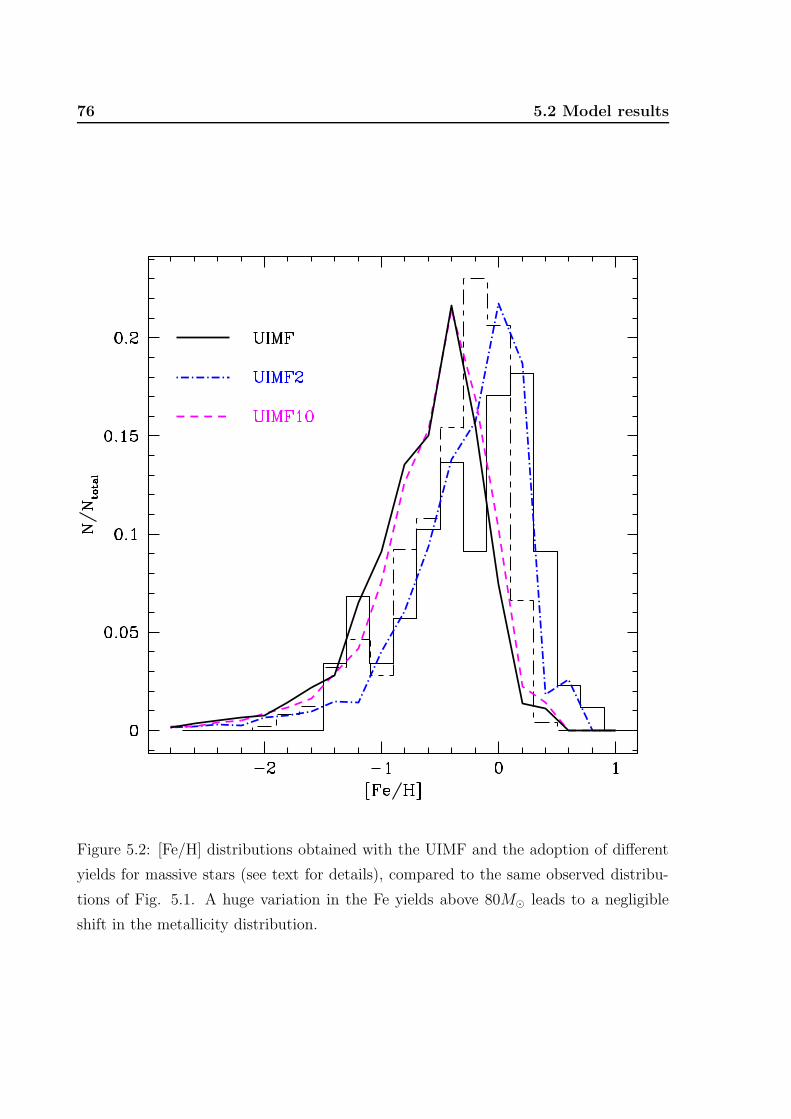
76 5.2 Model results
Figure 5.2: [Fe/H] distributions obtained with the UIMF and the adoption of different
yields for massive stars (see text for details), compared to the same observed distribu-
tions of Fig. 5.1. A huge variation in the Fe yields above 80M leads to a negligible
shift in the metallicity distribution.

Chapter 5. Universal or environment-dependent IMF? 77
Figure 5.3: Comparison of the observed metallicity distributions with those calculated
with the UIMF and with models that adopt different values for the star formation
efficiency (UIMF-νA and B) and the gas infall timescale (UIMF-τ). Namely, higher
values were chosen for τ and both higher and lower values for ν. Observations are the
same as in Fig. 5.1.
78 5.2 Model results
5.2.2 The effect of other evolutionary parameters
The main contributors to the chemical enrichment in the bulge are Type II supernovae,
which have massive progenitors, since the timescales of enrichment are so short. As a
consequence of that, Ballero et al. (2007a) predict overabundance of α-elements relative
to Fe for a wide range of [Fe/H]. It should be possible to obtain a larger enrichment from
Type Ia supernovae, which originate from low- and intermediate-mass stars, by adjusting
other parameters that have an effect on chemical evolution, such as the star formation
efficiency ν or the infall timescale τ . Therefore, we also investigated two more models:
Model UIMF-νA, where we set ν = 5 Gyr−1, and Model UIMF-τ , where τ = 0.25
Gyr. The star formation and gas consumption in this case should be slower, giving
Type Ia supernovae more time to enrich the interstellar medium with Fe. However, it
should be possible to enhance the Fe production by increasing the contribution of Type
II supernovae with a faster enrichment, i.e. increasing the star formation efficiency;
therefore, we also considered Model UIMF-νB, where ν = 50 Gyr−1.
We see in Fig. 5.3, however, that the attempt to shift the position of the metallicity
distribution by means of a change in these parameters is not successful, as already shown
in Ballero et al. (2007a) since they mainly act on the broadness of the distribution.
In the case of a very high star formation efficiency, the effect can be explained if we
consider that gas consumption occurs very rapidly and that stars are no longer formed
after a very short time. On the other hand, since the enrichment is very fast, there is
a lack of metal-poor stars. The opposite occurs in the case of a lower star formation
efficiency. In the case of different timescales of infall, the peak is actually shifted, as
can be seen from the figure, but the correct shape of the metallicity distribution is
not preserved. This is because, if the gas is accreted more slowly, the number of stars
produced at low metallicities is lower, so the calculated metallicity distribution gets
sharper.
5.2.3 Results for M31
Fig. 5.4 shows the metallicity distributions resulting from our reference model and the
model with the UIMF compared to the metallicity distribution of M31 as measured
by Sarajedini & Jablonka (2005) translating the observed colour-magnitude diagram at
∼ 1.6 kpc (G170 bulge field) from the centre into a metallicity distribution function by
means of red giant branches with various metallicities. This metallicity distribution,

Chapter 5. Universal or environment-dependent IMF? 79
Figure 5.4: [Fe/H] distribution function for the G170 field of the M31 bulge (histogram)
measured by Sarajedini & Jablonka (2005) compared with the results of our reference
model (Ballero et al. 2007a) and of the UIMF model. We also show the results of model
MB90, which is intermediate between the two and provides the best fit to the observed
metallicity distribution.

80 5.2 Model results
though still consistent with the ones of the Galactic bulge and therefore indicating a
similar enrichment history of the two bulges, is slightly more metal-poor on average and
is compatible with both the reference model and the model with the UIMF; however,
we also plotted the metallicity distribution calculated with x2 = 1.1, like in Matteucci
& Brocato (1990, model MB90), which gives the best fit. In any case, we can safely
conclude that an IMF with x ∼ 1 is more suitable for galactic bulges than the UIMF.
5.2.4 Discussion
Other possibilities that could affect the chemical evolution have not been investigated.
The lower mass cutoff Minf of the IMF is constrained by measurements in the bulge
field and cluster giant stars (Kuijken & Rich 2002; Zoccali et al. 2003; Rich & Origlia
2005) that indicate that the bulk of them is roughly 10 Gyr old; therefore, the value of
the lowest mass cutoff cannot be higher than ∼ 1M. No difference is expected to arise
if we increase Minf to that value, since stars below 1M have not yet contributed to
the bulge enrichment. Furthermore, it has already been shown by Ballero et al. (2006)
that the adoption of a mass cutoff of 10M for the so-called Population III stars up to
a metallicity suitable for the formation of these stars (i.e. Z ' 10−8 − 10−4; Bromm
& Larson 2004) has almost no effect on the predicted metallicity distribution, and even
less in the bulge since such metallicities are reached in a very short time.
Lowering the SFR with the UIMF/IGIMF models in the bulge and accreting popu-
lations with supersolar metallicity, such as are evident in the ancient super-metal-rich
open cluster NGC6791 (Salaris et al. 2004), or accreting supersolar gas may be able to
match the observed metallicity distribution in the bulges of the Milky Way and M31.
This scenario would avoid changing the IMF, but would also imply substantial accretion
events in the build-up of bulges. Such accretion episodes are likely to modify the [α/Fe]
vs. [Fe/H] plots at variance with observations. Due to the stochastic nature of mergers,
each of them would introduce a wide spread in the plots, which is not observed. Con-
tinuous outflows have the effect of lowering the effective yields (see Tosi et al., 1998)
and thus cannot be invoked to reproduce the observed metallicity distribution with the
adoption of the UIMF.

Chapter 5. Universal or environment-dependent IMF? 81
Observed distribution M µ σ
Zoccali et al. (2003, MW) −0.2 −0.397 0.444
Fulbright et al. (2006, MW) +0.2 −0.248 0.523
Sarajedini & Jablonka (2005, M31) −0.2 −0.369 0.438
Models
Ref. Model +0.0 −0.297 0.502
UIMF −0.4 −0.632 0.501
IGIMF −0.6 −0.896 0.494
UIMF2 +0.0 −0.272 0.514
UIMF10 −0.4 −0.580 0.493
MB90 −0.2 −0.447 0.493
UIMF-νA −0.4 −0.481 0.587
UIMF-νB −0.4 −0.599 0.503
UIMF-τ −0.2 −0.550 0.417
Table 5.1: Statistical properties of the measured (upper part) and calculated (lower
part) metallicity distributions of galactic bulges.
5.3 Summary and conclusions
We have tested the possibility of the UIMF of Kroupa (2001) or the “maximal” IGIMF
of Weidner & Kroupa (2005) as plausible ones in the bulge of our galaxy and of M31.
To this purpose, we included those IMFs in the chemical evolution model discussed in
Chapter 3 (Ballero et a. 2007a), which well reproduces the properties of the Galactic
bulge. The upper mass limit was extended to 150M in agreement with late findings
(Weidner & Kroupa 2004; Oey & Clarke 2005; Figer 2005; Koen 2006), and the stellar
yields of Francois et al. (2004) were extrapolated up to that mass. An attempt to
constrain the yields above 80M by assuming a priori the validity of the UIMF was
also made, and other parameters such as the star formation efficiency or infall timescale
were varied in order to achieve a better fit.
Table 5.1 summarises the statistical properties of the observed and calculated distri-
butions. The first column shows the reference or the model name; the second column
reports the position of the peak on the [Fe/H] axis, i.e. the mode M; and in the third
and fourth columns the average µ and the standard deviation σ of the considered dis-
tribution are shown, respectively. Together with the reference, it is indicated whether it
applies to the Milky Way or M31 bulge. It was found that it is not possible to reproduce

82 5.3 Summary and conclusions
in a satisfactory way the observed metallicity distributions of the Galactic bulge and
of M31 with the UIMF, which has a Salpeter (1955) index above 0.5M, because the
predicted metallicity distribution is too metal-poor. The adoption of the IGIMF, which
has a Scalo (1986) index above 1M, worsens the agreement further. This highlights the
fact that the main Fe contributors in galactic bulges are Type II supernovae, since the
timescales of enrichment are so short. Changing the nucleosynthesis prescriptions does
not have remarkable effects, unless very unrealistic assumptions about the stellar yields
of all massive stars are made. Even dramatic changes of yields above 80M do not basi-
cally affect the calculated distribution. We thus do not exclude the possibility of a higher
mass-cutoff, but show that it is impossible to put constraints on it based on chemical
abundances, since the weight in the IMF of stars in the mass range 80 < m/M < 150
is negligible.
Changes in ν and τ do not lead to any improvement because they mainly have an
effect on the breadth of the distribution and not on the position, which is governed
by the adopted IMF. This clearly indicates that, if the bulges of the Galaxy and M31
formed inside-out through the accretion of very metal-poor gas, a variation in the stellar
IMF is necessary among different environments and that an IMF index around x ∼ 1,
flatter than that of the UIMF, is preferable for galactic bulges. Theoretically speaking,
as already discussed in §3.4, this can be explained if we note that the star formation
in bulges proceeds like in a burst (see Elmegreen 1999); there are suggestions in the
literature (e.g. Baugh et al. 2005; Nagashima et al. 2005; Okamoto et al. 2005) about
a top-heavy IMF in starbursts. Figer (2005) also finds a flat IMF in the Arches cluster
near the Galactic centre (however, see also Kim et al. 2006).

Chapter 6
Chemical evolution of Seyfert
galaxies and bulge photometry
6.1 The co-evolution of AGNs and spheroids
The outstanding question of the co-evolution of active galactic nuclei (AGNs) and their
host galaxies has received considerable attention in the past decades, since various pieces
of evidence have pointed to a link between the formation of supermassive black holes
and the formation and evolution of their host spheroids: for example, the usual presence
of massive dark objects at the centre of nearby spheroids (Ford et al. 1997; Ho 1999;
Wandel 1999); the correlation between the black hole mass and the stellar velocity
dispersion of the host (for quiescent galaxies, Ferrarese & Merritt 2000; Gebhardt et
al. 2000a; Tremaine et al. 2002; for active galaxies, Gebhardt et al. 2000b; Ferrarese
et al. 2001; Shields et al. 2003; Onken et al. 2004; Nelson et al. 2004) or its mass
(Kormendy & Richstone 1995; Magorrian et al. 1998; McLure & Dunlop 2002; Marconi
& Hunt 2003; Dunlop et al. 2003; Haring & Rix 2004); the similarity between the light
evolution of QSO population and the star formation history of galaxies (Cavaliere &
Vittorini 1998; Haiman et al. 2004); the establishment of a good match among the
optical QSO luminosity function, the luminosity function of star-forming galaxies and
the mass function of dark matter halos at z ∼ 3 (Haenhelt et al. 1998).
As we said in §1.3, the most widely accepted explanation for the luminosity emitted
by an AGNs is radiatively efficient gas accretion onto a central supermassive black
hole. The outflows from AGNs can profoundly affect the evolution of the host galaxy,
e.g. by quenching or inducing the star formation (e.g., see Ciotti & Ostriker 2007, and

84 6.1 The co-evolution of AGNs and spheroids
references therein). The mutual feedback between galaxies and QSOs was used as a key
to solving the shortcomings of the semianalytic models in galaxy evolution, e.g. the
failure to account for the surface density of high-redshift massive galaxies (Blain et al.
2002; Cimatti et al. 2002) and for the α-enhancement as a function of mass (Thomas
et al. 2002), since it could provide a way to invert the hierarchical scenario for the
assembly of galaxies and star formation (see e.g. Monaco et al. 2000; Granato et al.
2004; Scannapieco et al. 2005).
The chemical abundances of the QSOs were first studied by Hamann & Ferland
(1993), who combined chemical evolution and spectral synthesis models to interpret
the N v/C iv and N v/He ii broad emission line ratios and found out that the high
metallicities and the abundance ratios of the broad-line region are consistent with the
outcomes of the models for giant elliptical galaxies (Arimoto & Yoshii 1987; Matteucci
& Tornambe 1987; Angeletti & Giannone 1990), where the timescales of star formation
and enrichment are very short, and the IMF is top-heavy. In the same year, Padovani
& Matteucci (1993) and Matteucci & Padovani (1993) employed the chemical evolution
model of Matteucci (1992) to model the evolution of radio-loud QSOs, which are hosted
by massive ellipticals, following in detail the evolution of several chemical species in
the gas. They supposed that the mass loss from dying stars after the galactic wind
provides the fuel for the central black hole and modeled the bolometric luminosity as
Lbol = ηMc2, with a typical value for the efficiency of η = 0.1, and were successful in
obtaining the estimated QSO bolometric luminosities and the observed ratio of AGN to
host galaxy luminosity. Then, they studied the evolution of the chemical composition
of the gas lost by stars in elliptical galaxies and spiral bulges for various elements (C,
N, O, Ne, Mg, Si and Fe) and found out that the standard QSO emission lines were
naturally explained by the high SFR of spheroids at early times.
The relatively weak observed time dependence of the QSO abundances for t & 1 Gyr
was also predicted. The model of Matteucci & Padovani (1993) still followed the classic
wind scenario, where the efficiency of star formation decreases with increasing galactic
mass and which was found to be inconsistent with the correlation between spheroid mass
and α-enhancement (Matteucci 1994). Moreover, Padovani & Matteucci (1993) had to
assume that the accretion onto the black hole would not last longer than ∼ 108 years in
order to avoid excessively large final black hole masses.
Other works (Friaca & Terlevich 1998; Romano et al. 2002; Granato et al. 2004),
which had a more refined treatment of gas dynamics, limited their analysis of chemical

Chapter 6. Chemical evolution of Seyferts and bulge photometry 85
abundances to the metallicity Z and the [Mg/Fe] ratio and their correlation with the
galactic mass.
All these studies were mainly devoted to studying the co-evolution of radio-loud
QSOs and their host spheroids, which are elliptical galaxies. We extended (Ballero
et al. 2008) the approach of Padovani & Matteucci (1993) to AGNs hosted by spiral
bulges, using our chemical evolution model for the bulge as a baseline model with the
introduction of the treatment of feedback from the central black hole and a more sophis-
ticated way of dealing with the accretion rate. Since Seyfert nuclei tend to be hosted
by disk-dominated galaxies, our study was applied to this class of objects.
6.2 Observations of abundances in QSOs and Seyfert
galaxies
Estimates of chemical abundance ratios in AGNs are not an easy task. The use of
emission lines is subject to large uncertainties due to the dependence of the lines on
several parameters that are difficult to quantify (e.g. column density, microturbulence,
collisional excitation, etc.). This is a problem since most measurements of the [Fe/Mg]
abundance ratio, which provides a clock for constraining the ages of QSOs and their
timescales of enrichment, rely on the flux ratio of the Fe ii (UV bump) and Mg ii (λ2800)
emission lines. The true physical origin of the Fe ii UV complex was questioned by
Verner et al. (2003), Baldwin et al. (2004) and Korista et al. (2004), who show that the
flux ratio does not scale directly with the abundance ratio due to the thermostatic effect
of coolants. Absorption lines could be a better probe of QSO environments, especially
narrow absorption lines that avoid saturation and blending of important abundance
diagnostics. However, these data require large signal-to-noise ratios and are therefore
harder to obtain. Moreover, they are not free from uncertainties concerning the shape
of ionising spectrum, the lack of ionisation constraints, the unknown coverage fraction
and the exact location of the absorbers (see Hamann & Ferland, 1999 for an extensive
review about QSO abundance diagnostics).
Given these caveats, it is evident, in any case, that the emission spectrum of AGNs
is particularly alike for a very wide range of redshifts and luminosities (Osmer & Shields
1999). The most probable explanation is a similarity of chemical abundances. In par-
ticular, the analysis of the Fe ii(UV bump)/Mg ii(λ2800) flux ratio in various redshift
ranges (Thompson et al. 1999; Iwamuro et al. 2002; Freudling et al. 2003; Dietrich et

86 6.2 Observations of abundances in QSOs and Seyfert galaxies
al. 2003a; Barth et al. 2003; Maiolino et al. 2003; Iwamoto et al. 2004) is consistent
with an [Fe/Mg] abundance ratio that is slightly supersolar and almost constant out to
z ∼ 6.4. This result was also confirmed for z ∼ 6 QSOs by very recent works (Kurk et al.
2007; Jiang et al. 2007). A weak trend with luminosity has been detected (Dietrich et
al. 2003a). Due to the time delay necessary for Fe enrichment from Type II supernovae
in a star formation history typical of elliptical galaxies (see Matteucci & Recchi 2001),
this means that the surrounding stellar population must already be in place by the time
the AGN shines and that, in a well-mixed interstellar medium, star formation must have
begun & 108 years before the observed activity, i.e. at redshifts zf & 10 (Hamann et al.
2002; Hamann et al. 2004).
Many efforts have been devoted to the measurement of nitrogen lines, since due to
its secondary nature, the N abundance relative to its seed nuclei (e.g. oxygen) is a good
proxy for metallicity. As abundance indicators, broad emission line ratios of N v/C iv
and N v/He ii were analysed by Hamann & Ferland (1993). Hamann & Ferland (1999)
also indicated N v/C iv and N v/O vi in narrow absorption line systems as possible
abundance indicators. More recently, Hamann et al. (2002) favour N iii]/O iii] and
N v/(C iv + O vi) as the most robust abundance indicators. The general conclusions
drawn from these diagnostics are that the AGNs appear to be metal rich at all observed
redshifts, with metallicities ranging from solar up to ∼ 10 times solar. Dietrich et
al. (2003b) studied a sample of 70 high-redshift QSOs (3.5 . z . 5.0) and, based
on emission-line flux ratios involving C, N, O and He, estimated an average overall
metallicity of ∼ 4 − 5Z for the emitting gas. A similar estimate (∼ Z) was drawn
more recently by Nagao et al. (2006), who examined 5344 spectra of high-redshift
(z ≥ 2) QSOs taken from the SDSS DR2; they also confirm the detected trend in the
N/He and N/C emission line ratios, which suggests that there might be a correlation
with luminosity, i.e. more luminous QSOs, residing in more massive galaxies, are more
metal rich. Bentz et al. (2004) suggested that some very nitrogen-enriched QSOs
may be caught at the peak of metal enrichment, e.g. near the end of their accretion
phases, although their conclusions are not definite. Work carried out on intrinsic narrow
absorption line systems (Petitjean & Srianand 1999; Hamann et al. 2003; D’Odorico
et al. 2004) confirms that the observed N, C and Si abundance ratios are consistent
with at least solar metallicities. In particular, D’Odorico et al. (2004) interpreted their
observations as suggestive of a scenario of rapid enrichment due to a short (∼ 1 Gyr)
star formation burst. The amount of emission from dust and CO in high-redshift QSOs

Chapter 6. Chemical evolution of Seyferts and bulge photometry 87
(Cox et al. 2002) corroborate the idea of massive amounts of star formation preceding
the shining of the AGN. However, there is no need for exotic scenarios to explain the
production of heavy elements near QSOs (e.g. central star clusters, star formation inside
accretion disks), since normal chemical evolution of ellipticals is sufficient to this purpose
(Hamann & Ferland 1993; Matteucci & Padovani 1993).
The majority of conclusions concerning QSOs has been found to hold also for Seyfert
galaxies, i.e. observations seem to confirm that most Seyfert galaxies are metal rich.
An overabundance of nitrogen by a factor ranging from about 2 to 5 was first detected
in the narrow line region of Seyferts by Storchi-Bergmann & Pastoriza (1989, 1990),
Storchi-Bergmann et al. (1990) and Storchi-Bergmann (1991), and was later confirmed
by Schmitt et al. (1994). Further work by Storchi-Bergmann et al. (1996) allowed
them to derive the chemical composition of the circumnuclear gas in 11 AGNs, and high
metallicities were found (O ranging from solar to 2 − 3 times solar and N up to 4 − 5
times solar). This trend was also measured in more recent works (Wills et al. 2000;
Mathur 2000). Fraquelli & Storchi-Bergmann (2003) examined the extended emission
line region of 18 Seyferts and claimed that the range in the observed [N ii]/[O ii] line
ratios can only be reproduced by a range of oxygen abundances going from 0.5 to 3 times
solar. By a means of a multi-cloud model, Rodrıguez-Ardila et al. (2005) deduce that a
nitrogen abundance higher than solar by a factor of at least two would be in agreement
with the [N ii]+/[O iii]+ line ratio observed in the narrow line Seyfert 1 galaxy Mrk 766.
Finally, Fields et al. (2005a) use a simple photoionization model of the absorbing gas to
find that the strongest absorption system of the narrow line Seyfert 1 galaxy Mrk 1044
has N/C & 4(N/C).
In the circumnuclear gas of the same galaxy, using column density measurements of
O vi, C iv, N v and H i, Fields et al. (2005b) claimed that the metallicity is about
5 times solar. This is consistent with expectations from previous studies. Komossa &
Mathur (2001), after studying the influence of metallicity on the multi-phase equilibrium
in photoionized gas, stated that in objects with steep X-ray spectra, such as narrow line
Seyfert 1 galaxies, such an equilibrium is not possible if Z is not supersolar. Studying
forbidden emission lines, Nagao et al. (2002) derived Z & 2.5Z in narrow line Seyfert 1
galaxies, whereas the gas of broad line Seyferts tends to be slightly less metal rich.
An overabundance of iron was suggested to explain the strong optical Fe ii emission
in narrow line Seyferts (Collin & Joly 2000) and could provide an explanation for the
absorption features around ∼ 1 keV seen in some of these galaxies (Ulrich et al. 1999;

88 6.3 Building models for other bulges
Mb (M) ν (Gyr−1) Re (kpc) tGW (Gyr)
2 × 10⁹ 11 1 0.31
2 × 10¹⁰ 20 2 0.27
1011 50 4 0.22
Table 6.1: Features of the examined models, in order: bulge mass, star formation ef-
ficiency, bulge effective radius. The table also reports the time of occurrence of the
galactic wind.
Turner et al. 1999) or for the strength of the FeKα lines (Fabian & Iwasawa 2000).
By constraining the relationship between iron abundance and reflection fraction, Lee
et al. (1999) show that the observed strong iron line intensity in the Seyfert galaxy
MCG−6-30-15 is explained by an iron overabundance by a factor of ∼ 2 in the accretion
disk. Ivanov et al. (2003) find values for [Fe/H] derived from the Mg i 1.50µm line
ranging from −0.32 to +0.49, but these values were not corrected for dilution effects
from the dusty torus continuum, so are probably underestimated.
6.3 Building models for other bulges
We recall that, in our reference model (Ballero et al. 2007a), the parameters that allow
a best fit of the metallicity distributions and the [α/Fe] vs. [Fe/H] ratios measured in
the bulge giants are the following: ν = 20 Gyr−1, τ = 0.1 Gyr, and two slopes for
the IMF, namely x1 = 0.33 for 0.1 ≤ m/M ≤ 1 (in agreement with the photometric
measurements of Zoccali et al. 2000) and x2 = 0.95 for 1 ≤ m/M ≤ 80. We also
consider the case x2 = 1.35 (Salpeter 1955) for comparison.
This model holds for a galaxy like ours with a bulge of Mb = 2 × 10¹⁰M. We are
going to predict the properties of Seyfert nuclei hosted by bulges of different masses,
therefore some model parameters will have to be re-scaled. We choose to keep the IMF
constant and to scale the effective radius and the star formation efficiency following the
inverse-wind scenario (Matteucci 1994). The possibility of changing the infall timescale
with mass is not explored for the moment. Table 6.1 reports the adopted parameters
for each bulge mass.

Chapter 6. Chemical evolution of Seyferts and bulge photometry 89
6.4 Photometry of bulges
By matching chemical evolution models with a spectro-photometric code, it has been
possible to reproduce the present-day photometric features of galaxies of various mor-
phological types (Calura & Matteucci 2006; Calura et al. 2007b) and to perform detailed
studies of the evolution of the luminous matter in the Universe (Calura & Matteucci
2003; Calura et al. 2004). By means of the chemical evolution model plus a spectro-
photometric code, we are now attempting to model the photometric features of galactic
bulges. All the spectro-photometric calculations are performed by means of the code
developed by Jimenez et al. (2004) and based on the stellar isochrones computed by
Jimenez et al. (1998) and on the stellar atmospheric models by Kurucz (1992). The
main advantage of this photometric code is that it allows to follow in detail the metal-
licity evolution of the gas, thanks to the large number of simple stellar populations
calculated by Jimenez et al. (2004) by means of new stellar tracks, with ages between
106 and 1.4 × 10¹⁰ yr and metallicities ranging from Z = 0.0002 to Z = 0.1.
Starting from the stellar spectra, we first build simple stellar population models
consistent with the chemical evolution at any given time and weighted according to
the assumed IMF. Then, a composite stellar population consists of the sum of different
simple stellar populations formed at different times, with a luminosity at an age t0 and
at a particular wavelength λ given by
Lλ(t0) =
∫ t0
0
∫ Zf
Zi
ψ(t0 − t)LSSP,λ(Z, t0 − t)dZdt, (6.1)
where the luminosity of the simple stellar population can be written as
LSSP,λ(Z, t0 − t) =
∫ Mmax
Mmin
φ(m)lλ(Z,m, t0 − t)dm (6.2)
and where lλ(Z,m, t0 − t) is the luminosity of a star of mass m, metallicity Z and age
t0 − t; Zi and Zf are the initial and final metallicities, Mmin and Mmax are the lowest
and highest stellar masses in the population, φ(m) is the IMF and ψ(t) is the SFR at
the time t. Peletier et al. (1999) have shown that dust in local bulges is very patchy
and concentrated in the innermost regions, i.e. within distances of ∼ 100 pc. They also
showed that dust extinction effects are negligible at distances of ∼ 1Reff . In addition,
we compared our photometric predictions to observational results largely unaffected
by dust, such as the ones by Balcells & Peletier (1994). For these reasons, in all our
spectro-photometric calculations, we do not take dust extinction into account.
90 6.5 Energetics of the interstellar medium
The photometrical evolution of actual Seyfert galaxies, which requires modelling of
the AGN continuum and, for Type 2 Seyferts, of the dusty torus, is not treated at
present and may be the subject of a future investigation.
6.5 Energetics of the interstellar medium
In Chapter 2, we calculated the binding energy ∆Eg of the bulge gas following Bertin
et al. (1992), i.e. by treating the bulge as a scaled-down two-component elliptical (thus
ignoring the disk contribution). We also assumed that the thermal energy of the bulge
interstellar medium was mainly contributed by the explosion of Type Ia and Type II
supernovae. In the present exploration, not only do we adopt a more realistic disk galaxy
model to better estimate the binding energy of the gas in the bulge, but we also consider
the additional contribution to the gas thermal energy given by the black hole feedback,
so that
Eth(t) = Eth,SN(t) + Eth,AGN(t) (6.3)
The various simplifying assumptions adopted in the evaluation of the gas binding
energy and of the black hole feedback will be discussed in some detail in the follow-
ing sections. The gas binding energy and thermal energy which are calculated in the
next subsections will then be compared as in Eq. 2.9 in order to estimate the time of
occurrence of the galactic wind.
6.5.1 The binding energy
If we define
Ψ(r, t) = πR2eψ(r, t) (6.4)
(i.e. the volume SFR) and
M∗ =
∫ 80
0.1
φ(m)Ψ(r, t− τm)Rm(t− τm)dm (6.5)
where Rm is the return mass fraction (i.e. the fraction of mass in a stellar generation
that is ejected into the interstellar medium by stars of mass m; see Tinsley 1980) and
τm is the lifetime of a star of mass m, then, before the galactic wind, the mass of gas in
the bulge evolves at a rate
Mg(t < tGW ) = Minf + M∗ − Ψ(r, t) − MBH ; (6.6)

Chapter 6. Chemical evolution of Seyferts and bulge photometry 91
i.e. gas is accreted from the halo, is returned by stellar mass loss, and is subtracted by
star formation and black hole accretion. After the wind, star formation vanishes and we
suppose that the infall is arrested due to the development of a global outflow. Therefore,
this equation reduces to
Mg(t > tGW ) = M∗ − MBH − MW (6.7)
where MW is the rate of mass loss due to the galactic wind. We assume that all the
gas present at a given time is lost, so that MW = M∗ − MBH . In the present treatment
the galaxy mass model is required in order to estimate the binding energy of the gas in
the bulge, a key ingredient in establishing of the wind phase. In particular, the current
galaxy model is made by three different components, namely:
- A spherical Hernquist (1990) distribution representing the stellar component of
the bulge:
ρb(r) =Mb
2π
rb
r(r + rb)3,
Φb(r) = − GMb
r + rb
(6.8)
where Mb is the bulge mass, Φb the bulge potential and rb the scale radius of the
bulge, related to its effective radius by the relation Re ' 1.8rb.
- A spherical isothermal dark matter halo with circular velocity vc:
ρDM (r) =v2
c
4πGr2
ΦDM (r) = v2c ln
r
r0
(6.9)
where r0 is an arbitrary scale-length.
- A razor-thin exponential disk with surface density
Σd(R) =Md
2πR2d
e−R/Rd (6.10)
where Md is the total disk mass, R the cylindrical radius, and Rd the disk scale
radius. As is well known, the gravitational potential of a disk can in general
be expressed by using the Hankel-Fourier transforms (e.g. Binney & Tremaine
1987): however, as shown in Appendix, under the assumption of a spherical gas
distribution, the contribution to the gas binding energy can be easily calculated
without using the explicit disk potential.

92 6.5 Energetics of the interstellar medium
In fact, we assume that the gas distribution before the establishment of the galactic
wind is spherically symmetric and parallel to the stellar one; i.e.
ρg(r) =Mg
2π
rb
r(r + rb)3. (6.11)
In order to estimate the energy required to induce a bulge wind, we define a displace-
ment radius rt, and we calculate the energy required to displace at rt the gas contained at
r < rt (while maintaining spherical symmetry). We adopt a reference value of rt = 3Re;
the calculated values of the binding energy do not change significantly for rt ranging
from 2Re to 10Re. A spherically symmetric displacement (while not fully justified the-
oretically) allows a simple evaluation of the gas binding energy, and it is acceptable in
the present approach. Consistent with the assumption above,
∆Eg = ∆Egb + ∆EgDM + ∆Egd (6.12)
where the various terms at the right hand side describe the gas-to-bulge, gas-to-dark
matter and gas-to-disk contributions. Elementary integrations show that
∆Egb = 4π
∫ rt
0
ρg(r)[Φb(rt) − Φb(r)]r2dr =
GMgMb
rb
δ3
3(1 + δ)3(6.13)
and
∆EgDM = 4π
∫ rt
0
ρg(r)[ΦDM(rt) − ΦDM (r)]r2dr = Mgv2c
[ln(1 + δ) − δ
1 + δ
](6.14)
where δ ≡ rt/rb, while
∆Egd =GMgMd
Rd× ∆Egd (6.15)
and the function ∆Egd is given in Appendix. Of course, ∆Eg is linearly proportional to
the gas mass in the bulge.
In Fig. 6.1 we see that, for a 1010M bulge like ours, the dominant contribution arises
from the dark matter halo, whereas the bulge and disk contributions are comparable,
both about one order of magnitude smaller than the dark matter halo one. This differs
from previous calculations (Ballero et al. 2007a) in the way that the bulge contribution
is reduced by almost one order of magnitude. The same is true of the bulges of other
masses. We must consider, moreover, that in the inside-out scenario for the Galaxy
formation (Chiappini et al. 1997) the disk will probably form much later than the
bulge, so its contribution to the potential well during the bulge formation could be
negligible. Thus, what we explore is the extreme hypothesis that the disk has been in
place since the beginning of the bulge evolution.

Chapter 6. Chemical evolution of Seyferts and bulge photometry 93
Figure 6.1: Time evolution of the different contributions to the gas binding energy in
the bulge of a Milky Way-like galaxy: dark matter halo (dashed line), bulge (dotted
line), and exponential disk (solid line). In particular, Mb = 2 × 10¹⁰M, Re = 2 kpc,
vc = 200 km/s, Md = 1011M and Rd = 4.3 kpc.

94 6.5 Energetics of the interstellar medium
6.5.2 Black hole accretion and feedback
In our phenomenological treatment of black hole feedback, we only considered radiative
feedback, thus neglecting other feedback mechanisms such as radiation pressure and
relativistic particles, as well as mechanical phenomena associated with jets. From this
point of view we are following the approach described in Sazonov et al. (2005), even
though several aspects of the physics considered there (in the context of elliptical galaxy
formation) are not taken into account. In fact, we note that these phenomena can only
be treated in the proper way by using hydrodynamical simulations.
We suppose that the bulge gas is fed into the spherically accreting black hole at the
Bondi rate MB. However, the amount of accreting material cannot exceed the Eddington
limit, i.e.:
MBH = min(MEdd, MB). (6.16)
The Eddington accretion rate, i.e. the accretion rate beyond which radiation pressure
overwhelms gravity, is given by
MEdd =LEdd
ηc2(6.17)
where η is the efficiency of mass-to-energy conversion. In general, 0.001 ≤ η ≤ 0.1, and
we adopt the maximum value η = 0.1 (Yu & Tremaine 2002). The Eddington luminosity
is given by
LEdd = 1.3 × 1046 MBH
108M
erg s−1. (6.18)
The Bondi accretion rate describes the stationary flow of gas from large distances
onto the black hole, for a given gas temperature and density (see Bondi 1952), and is
given by
MB = 4πR2BρBcS, (6.19)
where
RB =GMBHµmp
2γkT= 16 pc
1
γ
MBH
108M
(T
106K
)−1
(6.20)
with
c2s =
(∂p
∂ρ
)
isot
=kT
µmp
, (6.21)
and ρB (the gas density at RB) can be estimated as
ρB =ρe
3
(Re
RB
)2
. (6.22)

Chapter 6. Chemical evolution of Seyferts and bulge photometry 95
In the code we adopt γ = 1 (isothermal flow). If we assume that all the gas mass is
contained within 2Re, the mean gas density within Re is given by
ρe =3Mg
8πR3e
. (6.23)
The equilibrium gas temperature can be estimated as the bulge virial temperature.
Tvir 'µmpσ
2
k= 3.0 × 10⁶ K
(σ
200 km s−1
)2
, (6.24)
where σ is the one-dimensional stellar velocity dispersion in the bulge, which is given by
σ2 ≡ − Wb
3Mb. (6.25)
The virial potential trace Wb for the bulge is obtained by summing the contribution of
the three galaxy components, i.e.
Wb = Wbb +WbDM +Wbd = −GM2b
6rb−Mbv
2c −
GMdMbWbd
Rd(6.26)
where the term Wbd is given in Appendix.
The bolometric luminosity emitted by the accreting black hole is then calculated as
Lbol = ηc2MBH . (6.27)
Finally, we assume that the energy released by the black hole is the integral of a
fraction f of this luminosity over the time-step:
Eth,BH = f
∫ t+∆t
t
Lboldt ' fLbol∆t. (6.28)
The value of f can vary between 0 and 1; we assume f = 0.05 (Di Matteo et al. 2005).
The seed black hole mass was modified in a range 5 × 10² − 5 × 10⁴M without any
appreciable change in the results. Therefore, we adopt a universal seed black hole mass
of 103M.
6.6 Results
6.6.1 Mass loss and energetics
Fig. 6.2 shows the evolution of the Eddington and Bondi accretion rates. We can see
that the history of accretion onto the central black hole can be divided into two phases:

96 6.6 Results
Figure 6.2: Time evolution of the Eddington (dashed line) and Bondi (dot-dashed line)
accretion rates for bulges with various masses. The thicker lines indicate the resulting
accretion rate, which is assumed to be the minimum between the two. The break in the
Bondi rate corresponds to the occurrence of the galactic wind.

Chapter 6. Chemical evolution of Seyferts and bulge photometry 97
Figure 6.3: Energy balance as a function of time for bulges of various masses. The figure
shows the gas binding energy (solid line) compared to the thermal energy released by
supernovae (dashed line) and the accreting black hole (dot-dashed line). The break in
the binding energy and in the supernova feedback corresponds to the occurrence of the
galactic wind.

98 6.6 Results
the first, Eddington-limited, and the second, Bondi-limited. Most of the accretion and
fuelling occurs around the period of transition between the two phases, which coincides
approximately with the occurrence of the wind, although it extends for some time further
in the most massive models. The details of the transition depend on the numerical
treatment of the wind; however, since the gas consumption in the bulge is very fast and
the Bondi rate depends on the gas density, we can expect that the results would not
change significantly even if we modeled the galactic wind as a continuous wind. The
black hole mass is essentially accreted, within a factor of two, in a period ranging from
0.3 to 0.8 Gyrs, i.e. 2 to 6% of the bulge lifetime, which we assume to be 13.7 Gyr.
Fig. 6.3 compares the different contributions to the thermal energy, i.e. the feedback
from supernovae and from the AGN, with the potential energy. We see that only in
the case of Mb = 2 × 10⁹M does the black hole feedback provide a thermal energy
comparable to what is produced by the supernova explosions before the onset of the
wind (note that the Bondi accretion rate does not vanish even if the thermal energy
of the interstellar medium is greater than the potential energy, due to the fresh gas
provided by the stellar mass losses of the ageing stars in the bulge). Therefore, in
the context of chemical and photometrical evolution, the contribution of the black hole
feedback is negligible in most cases, unless we assume an unrealistically large fraction of
the black hole luminosity is transferred into the interstellar medium. This conclusion is
also supported by hydrodynamical simulations specifically designed to study the effects
of radiative black hole feedback in elliptical galaxies (Ciotti & Ostriker 1997, 2001, 2007;
Ostriker & Ciotti 2005). Also, Di Matteo et al. (2003) show that it is unlikely that black
hole accretion plays a crucial role in the general process of galaxy formation, unless there
is strong energetic feedback by active QSOs (e.g. in the form of radio jets).
6.6.2 Star formation rate
Fig. 6.4 shows the evolution of the global SFR in the bulge as a function of time and
redshift. The break corresponds to the occurrence of the galactic wind. The redshift was
calculated assuming a ΛCDM cosmology with H0 = 65 km s−1 Mpc−1, ΩM = 0.3 and
ΩΛ = 0.7, and a redshift of formation of zf ' 10. It is evident that, in the case of the
most massive bulges, it is easy to reach the very high SFRs of a few times 1000M/yr
inferred from observations at high redshifts (e.g. Maiolino et al. 2005). It is worth
noting that this result matches the statement of Nagao et al. (2006) very well, that the
absence of a significant metallicity variation up to z ' 4.5 implies that the active star

Chapter 6. Chemical evolution of Seyferts and bulge photometry 99
Figure 6.4: Star formation rate as a function of time and redshift for bulges with various
masses. The peak value of the Mb = 2 × 10⁹M case is ∼ 40M/yr.
100 6.6 Results
formation epoch of QSO host galaxies occurred at z & 7. There is evidence of some tiny
downsizing (star formation ceases at slightly earlier times for larger galaxies; see Table
6.1). We stress that we are making predictions about single galaxies and not about the
AGN population, and we only want to show that it is possible to achieve such high rates
of star formation in a few Myrs.
6.6.3 Black hole masses and luminosities
In Fig. 6.5 we show the final black hole masses resulting from the accretion as a func-
tion of the bulge mass. The predicted black hole masses are in good agreement with
measurements of black hole masses inside Seyfert galaxies (Wandel et al. 1999; Kaspi et
al. 2000; Peterson 2003). This is a valuable result, given the simplistic assumptions of
our model, since in this case we do not have to stop accretion in an artificial way as in
Padovani & Matteucci (1993); in fact, the black hole growth at late times is limited by
the available amount of gas, as described by Bondi accretion. The figure suggests an ap-
proximately linear relation between the bulge and black hole mass, as first measured by
Kormendy & Richstone (1995) and Magorrian et al. (1998). Therefore, Seyfert galaxies
appear to obey the same relationship as quiescent galaxies and QSOs, as already stated
observationally by Nelson et al. (2004).
There were claims for a non-linear relation between spheroid and black hole mass
(Laor 2001; Wu & Han 2001); however, measurements of Marconi & Hunt (2003) re-
established the direct proportionality between the spheroid mass Msph and MBH ,
MBH ' 0.0022Msph, (6.29)
also in good agreement with recent estimates from McLure & Dunlop (2002) and Dunlop
et al. (2003)
MBH ' 0.0012Msph (6.30)
and from Haring & Rix (2004)
MBH ' 0.0016Msph. (6.31)
The three relations of McLure & Dunlop (2002), Marconi & Hunt (2003) and Haring
& Rix (2004) are thus reported in the figure for comparison. The agreement between
measurements and predictions is rather good (within a factor of two).
In Fig. 6.6 we plot the predicted bolometric nuclear luminosities Lbol for the var-
ious masses, compared with luminosity estimates for the Seyfert population (see e.g.

Chapter 6. Chemical evolution of Seyferts and bulge photometry 101
Figure 6.5: Final black hole masses as a function of the bulge mass predicted by our
models (triangles). The short dashed-long dashed line represents the measured relation
of McLure & Dunlop (2002), the dotted line the one of Marconi & Hunt (2003) and the
dashed line the one of Haring & Rix (2004).
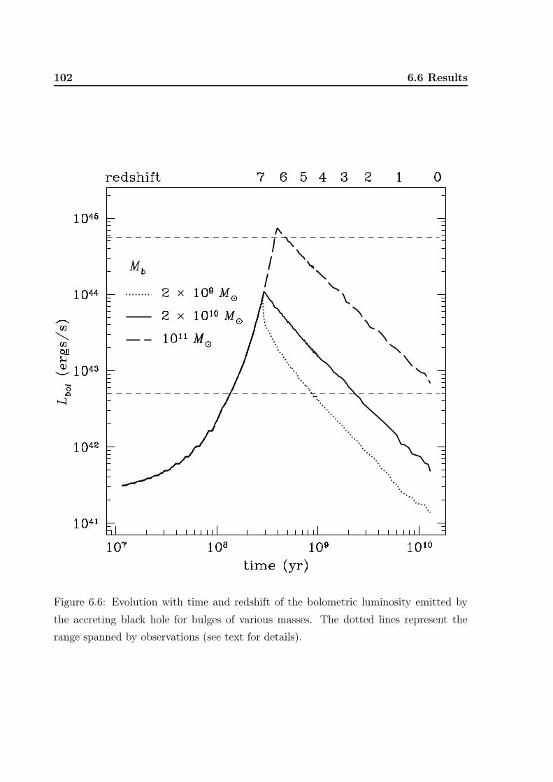
102 6.6 Results
Figure 6.6: Evolution with time and redshift of the bolometric luminosity emitted by
the accreting black hole for bulges of various masses. The dotted lines represent the
range spanned by observations (see text for details).
Chapter 6. Chemical evolution of Seyferts and bulge photometry 103
Gonzalez Delgado et al. 1998; Markowitz et al. 2003; Brandt & Hasinger 2005; Wang
& Wu 2005; Gu et al. 2006). Of course, Lbol is proportional to the calculated mass
accretion rate (Fig. 6.2). In the first part, the plots overlap because the Eddington lu-
minosity only depends on the black hole mass, and it is independent of the galaxy mass;
on the contrary, the Bondi accretion rate is sensitive to the galaxy features. The break
in the plot corresponds to the time when the Bondi accretion rate becomes lower than
the Eddington accretion rate (see Eqs. 6.17 and 6.19), and occurs later and later for
more massive galaxies, which therefore keep accreting at the Eddington rate on longer
timescales. This helps explain why the outcoming final black hole mass is proportional
to the adopted bulge mass.
We see that the luminosities near the maximum are reproduced by models of all
masses. The same is not true for local (z ' 0) Seyferts, because only the most massive
model yields a bolometric luminosity that lies in the observed range, while for other
masses the disagreement reaches a factor of ∼ 100. To simply shift the epoch of star
formation of the less massive Seyferts would require unrealistically young bulges (with
ages . 1 Gyr), whereas one of our main assumptions is that spiral bulges are old systems.
Padovani & Matteucci (1993) assumed that the black hole accreted the whole mass lost
from evolved stars. If we calculate the fraction MB/M∗ at any given time, we see that
its value is very close to 0.01. This explains why they obtained the correct nuclear
bolometric luminosity of local radio-loud QSOs, but severely overestimated the mass
of the resulting black hole, which led them to suggest that the accretion phase should
last for a period not longer than a few 108 years, at variance with the present work.
Moreover, it is not physically justified to assume that all the mass expelled from dying
stars falls onto the black hole.
One way to overcome this problem is to suppose that the smallest bulges undergo
a rejuvenation phase, which is possible because spiral bulges are not isolated systems,
but an interaction with their surrounding disks can be triggered in several ways (bar
instabilities, minor mergers, fly-by’s, and so on). By using models combining recent
star formation with a base old population, Thomas & Davies (2006) found that the
smallest bulges must have experienced star formation events involving 10 − 30% of
their total mass in the past 1 − 2 Gyr. The same conclusion was also reached on an
independent basis by MacArthur et al. (2007), who studied a sample of 137 spiral
bulges in the GOODS fields and, by means of photometric techniques, estimated the
star formation necessary to reproduce the observed colour range. They concluded that,

104 6.6 Results
while all stellar populations belonging to bulges with MB > 1011M are homogeneously
old and consistent with a single major burst of star formation at z > 2, the colours and
mass-to-light ratios of smaller bulges require that they have experienced mass growth
since z ∼ 1, so that a ∼ 10% fraction of stellar mass eventually goes into younger stars.
Secondary accretion/star formation episodes may also help explain the presence of
the Galactic bulge Mira population, whose calculated age is 1 − 3 Gyr (van Loon et al.
2003; Groenewegen & Blommaert 2005) and of young stars and star clusters in the very
centre of the Galaxy (Figer et al. 1999; Genzel et al. 2003). Paumard et al. (2006) also
studied a population of OB stars in the central parsec of the Galaxy and found an even
younger age of ' 6 ± 2 Myrs. A small fraction of intermediate-age stellar population
was also detected in Seyfert 2 nuclei (Sarzi et al. 2007).
Finally, we note that by means of the present (non-hydrodynamical) modelling of
the black hole accretion rate and of the gas budget, a truly realistic accretion cannot
be reproduced, whereas in a more realistic treatment, the AGN feedback would cause
the luminosity to switch on and off several times at the peaks of luminosity. We also
note that at late times, when the accretion is significantly sub-Eddington, a considerable
reduction in the emitted AGN luminosity might result as a consequence of a possible
radiatively inefficient accretion mode (e.g. Narayan & Yi 1994). This could reproduce
the quiescence of black holes at the centre of present-day inactive spiral galaxies in a
picture where all spiral galaxies host a Seyfert nucleus at some time of their evolution.
6.6.4 Metallicity and elemental abundances
The mean values attained by the metallicity and the examined abundance ratios for
z . 6 are resumed in Table 6.2. Note that all the [α/Fe] ratios are undersolar or solar.
Fig. 6.7 shows the evolution with time and redshift of the metallicity Z in solar units
(which, we recall, is the abundance of all the elements heavier than 4He), for a standard
ΛCDM scenario with H0 = 65 km s−1 Mpc−1, ΩM = 0.3 and ΩΛ = 0.7.
It can be seen that solar metallicities are reached in a very short time, ranging from
about 3 × 10⁷ to 108 years with decreasing bulge mass (see Table 6.2). We notice that,
due to the α-enhancement that is typical of spheroids prior to the wind, solar Z is always
reached well before solar [Fe/H] is attained, which occurs at times ∼ (1−3)×108 years.
Then, Z remains approximately constant for the contribution of Type Ia supernovae
and low- and intermediate-mass stars, before declining in the very late phases. The
high metallicities inferred from observations (e.g. Hamann et al 2002; Dietrich et al.
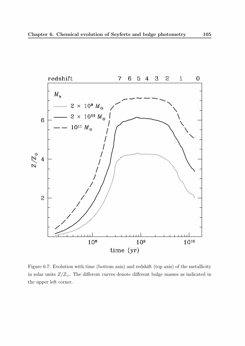
Chapter 6. Chemical evolution of Seyferts and bulge photometry 105
Figure 6.7: Evolution with time (bottom axis) and redshift (top axis) of the metallicity
in solar units Z/Z. The different curves denote different bulge masses as indicated in
the upper left corner.

106 6.6 Results
Chemical properties of Seyfert nuclei
Mb (M) 2 × 10⁹ 2 × 10¹⁰ 1011
Z/Z 4.23 6.11 7.22
[Fe/H] +0.83 +0.96 +1.07
[O/H] +0.18 +0.36 +0.48
[Mg/H] +0.38 +0.55 +0.69
[Si/H] +0.79 +0.98 +1.13
[Ca/H] +0.63 +0.88 +1.06
[O/Fe] −0.68 −0.60 −0.59
[Mg/Fe] −0.45 −0.41 −0.38
[Si/Fe] −0.04 +0.02 +0.06
[Ca/Fe] −0.19 −0.07 +0.00
[N/H] +0.28 +0.63 +0.87
[C/H] +0.15 +0.24 +0.30
[N/C] +0.13 +0.40 +0.57
t(Z) (yr) 108 6 × 10⁷ 3 × 10⁷
Table 6.2: Values assumed by the chemical abundance ratios and by the metallicity in
solar units after the wind by bulges of different masses, and the time by which Z is
reached in the different models (last line), are shown.
2003b, their Figures 5 and 6) are thus very easily achieved. More massive bulges give rise
to higher metallicities, which agrees with the statement that more luminous AGNs are
more metal rich, if we assume that more massive galaxies are also more luminous. This
assumption is supported observationally by e.g. Warner et al. (2003) who find a positive
correlation between the mass of the supermassive black hole and the metallicity derived
from emission lines involving N v in 578 AGNs spanning a wide range in redshifts.
The time dependencies of the abundances of the elements under study for each mass
are shown in the Figs. 6.8 (iron) and 6.9 (α-elements, carbon and nitrogen). A fast
increase in the abundances is noticeable at early times, as well as a weak decrease at later
times, for all the elements and all masses; after the galactic wind, i.e. for t & 0.2 − 0.3
Gyr (which corresponds to a redshift z ' 6−7 in the adopted cosmology) the abundances
decrease by a factor smaller than 2. Such a weak decrease occurs over a period of more
than 13 Gyr. This can explain the observed constancy of the QSO abundances as a
function of redshift (Osmer & Shields 1999).

Chapter 6. Chemical evolution of Seyferts and bulge photometry 107
Figure 6.8: Evolution with time (bottom axis) and redshift (top axis) of the [Fe/H]
abundance ratio in bulges of various masses, as indicated in the lower right corner.

108 6.6 Results
Figure 6.9: Evolution with time and redshift of the [X/H] abundance ratios for O, Mg,
Si, Ca, C and N in bulges of various masses. The bump at ∼ 2×10⁸ yr in the [Si/H] and
[Ca/H] plots is due to the occurrence of the wind, which shortly precedes the maximum
in the Type Ia supernova rate. The thin lines in the [N/H] plot represent the results
obtained by adopting primary N in massive stars, as in Matteucci (1986).

Chapter 6. Chemical evolution of Seyferts and bulge photometry 109
The elements can be divided according to their behaviour after the wind:
- O and Mg show moderate overabundances relative to solar. They are produced
essentially by massive stars (M > 8M) on short timescales (. 107 years), i.e.
almost in lockstep with the star formation. After the galactic wind, therefore,
their abundance cannot increase any more because star formation vanishes. They
tend instead to be diluted due to the effect of hydrogen-rich stellar mass loss from
dying stars. In our Galactic bulge model, at the time of the onset of the wind,
Mg is more abundant than O, since although [O/H] is higher at earlier times, it
declines very rapidly due to the dependence on metallicity of the adopted O yields
(Francois et al. 2004)1. Therefore, we expect the mean value attained by [O/H]
after the wind to be lower than that of [Mg/H], which is what we predict. In fact,
the mean [O/H] for z . 6 ranges from +0.18 to +0.48 dex, i.e. oxygen is ∼ 1.5
to 3 times solar, in good agreement with observations (Storchi-Bergmann et al.
1996; Fraquelli & Storchi-Bergmann, 2003), and the mean [Mg/H] ranges from
+0.38 to +0.69 dex (i.e. 2.5 to 5 times solar), depending on the mass of the host
bulge. Finally, we notice that both [O/H] and [Mg/H] reach solar values at times
closer to those when Z = Z with respect to [Fe/H] for the different models and
are therefore better proxies for the metallicity in the bulge. This is because the
metallicity is dominated by O in the bulge.
- Fe, Si and Ca are characterised by a bump immediately after the occurrence of the
galactic wind, which leads to a significant increase in their abundance, reaching
remarkably higher values than in the previous cases ([Fe/H]: +0.83 to +1.07, i.e.
∼7−10 times solar; [Si/H]: +0.79 to +1.13, i.e. ∼6−12 times solar; [Ca/H]: +0.63
to +1.06, i.e. ∼4−10 times solar). This bump is due to the combined effect of the
discontinuity caused by the onset of the galactic wind at times of 0.21 to 0.28 Gyr
depending on the model mass, and of the maximum of the Type Ia supernova rate,
occurring at ∼ 0.2 − 0.3 Gyr. In fact, these elements are also produced by Type
Ia supernovae (Fe mainly, Si and Ca in part, as they are also produced by Type II
supernovae), which derive from progenitors with masses ranging from 0.8 to 8M.
These elements are restored into the interstellar medium on timescales ranging
1Although, the Maeder (1992) yields for oxygen have been proved to solve the discrepancy be-
tween the abundance evolution of oxygen and other α-elements, in this Chapter we are still using the
Francois (2004) yields as standard since there are still open issues concerning the zero-point of the plots
(see Chapter 4).

110 6.6 Results
from ∼ 30 Myr to a Hubble time. Thus, their abundances could in principle keep
increasing even after the star formation has ceased. However, due to the adopted
top-heavy IMF (x2 = 0.95), a relatively small fraction of low- and intermediate-
mass stars were produced with respect to what we would expect if we had adopted
a steeper IMF (see below for a comparison with the IMF of Salpeter 1955), and
therefore what we observe is a decrease of the Si, Fe and Ca abundances after the
galactic wind. The estimates for Fe in Seyferts are lower than those calculated here,
but we must take several factors into account that would lead to underestimating
the Fe produced by stars, e.g. depletion by dust (see Calura et al. 2007a) or
dilution of spectra by a dusty torus continuum.
- C, as well as O and Mg, is slightly overabundant (∼1.3 to 2.7 times solar). Al-
though it is mostly produced by low- and intermediate-mass stars, in this same
range of masses it is also used up to form N. In this case the bump is less pro-
nounced and is mainly caused by the discontinuity induced by the galactic wind,
which enhances the relative contribution of low- and intermediate-mass stars.
- Finally, a behaviour similar to Fe is expected for N, since the bulk of this element
originates from stars with M < 8M. There are, nonetheless, two significant
differences: first, due its secondary nature, its abundance increases much more
rapidly than other elements with time (and with metallicity); and second, this very
rapid increase hides the bump at the onset of the wind. We also adopt a primary
N production in massive stars (Matteucci 1986; see also Chiappini et al. 2006),
but the effects of this choice are only visible before tGW , i.e. when nucleosynthesis
from massive stars is active; the decrease of the [N/H] ratio towards earlier times
(i.e. lower metallicities) is less rapid. Then, after the wind, the plots with and
without primary N essentially overlap. This has already been observed in Ballero
et al. (2006) and Ballero et al. (2007a). The mean values attained by [N/H] after
the galactic wind ranges from +0.28 to +0.87 dex; i.e., nitrogen is ∼2 to 8 times
overabundant with respect to solar. However, [N/H] reaches overabundances of
∼3−10 times solar at its peak. These results agree with the estimates for Seyferts
(Schmitt et al. 1994; Storchi-Bergmann et al. 1996; Rodrıguez-Ardila et al. 2005).
The different behaviour among the α-elements (O, Mg vs. Si, Ca) is even more
evident in Fig. 6.10, where the correlation with mass of the [α/Fe] abundance ratios
after the wind is shown. A net separation is present: whereas [Si/Fe] and [Ca/Fe] are

Chapter 6. Chemical evolution of Seyferts and bulge photometry 111
approximately solar, O and Mg are underabundant with respect to solar, O showing
a more pronounced underabundance. This also agrees with the estimates of a slightly
supersolar [Fe/Mg] in QSOs and of its weak correlation with luminosity (Dietrich et
al. 2003a). Since both [Fe/H] and [Mg/H] are constant within a factor of 2 up to high
redshifts (z ' 6) and follow the same declining trend with time, we expect this relation
to hold for most of the bulge lifetime, which is what is observed for QSOs (Thompson
et al. 1999; Iwamuro et al. 2002; Freudling et al. 2003; Dietrich et al. 2003a; Barth et
al. 2003; Maiolino et al. 2003; Iwamoto et al. 2004). Here, we predict [Fe/Mg] values
ranging from +0.38 to +0.45 dex, the highest values corresponding to less massive
galaxies where star formation stops later and Type Ia supernovae have more time to
pollute the bulge interstellar medium.
Fig. 6.11 shows the variation with mass in the [N/C] abundance ratio. The figure
illustrates well that this ratio is remarkably sensitive to the galaxy mass, which, as we
have seen in Fig. 6.7, is correlated with the galaxy metallicity. This happens because
of the secondary nature of N, which is produced at the expense of C in a fashion pro-
portional to the metallicity of the interstellar medium. The mean [N/C] ratio for z . 6
ranges from +0.13 to +0.57 dex depending on the bulge mass; i.e., the N/C ratio is ∼1.4 to 3.7 times solar. If we consider the amount of variation in the two abundances,
these values are consistent with the estimates of Fields et al. (2005a).
Finally, we briefly compare the results obtained with the top-heavy IMF (x2 = 0.95)
with those we obtain if instead we adopt x2 = 1.35 (Salpeter 1955). In Ballero et al.
(2007a) this IMF was excluded on the basis of the stellar metallicity distribution, since
with our model the Salpeter index for massive stars gives rise to a distribution that is
too metal-poor with respect to the observed ones (Zoccali et al. 2003; Fulbright et al.
2006), and Ballero et al. (2007b) seem to further confirm this point. However, Pipino et
al. (2007b) showed that the multi-zone hydrodynamical model for ellipticals of Pipino
et al. (2007a), where the spheroids form “outside-in”, can be adapted to the galactic
bulge and, by means of internal gas flows that funnel metals to the centre, it reproduces
the above-mentioned metallicity distributions with a Salpeter IMF (although the top-
heavy IMF with is still considered a viable solution). Furthermore, as we shall show
(see §6.6.5), the (B− I) colours and bulge K-band luminosity are better reproduced by
a Salpeter IMF above 1M. Therefore a brief comparison is useful.
In Fig. 6.12 we show the evolution with time and redshift of the abundance ratios
relative to hydrogen for some of the elements considered, namely Fe, O and N. We find

112 6.6 Results
Figure 6.10: Correlation with bulge mass of the [α/Fe] abundance ratios for z . 6.
Figure 6.11: Correlation with bulge mass of the [N/C] abundance ratio for z . 6.

Chapter 6. Chemical evolution of Seyferts and bulge photometry 113
Figure 6.12: Evolution with time and redshift of the [X/H] abundance ratios for Fe, O
and N in bulges of various masses and the adoption of a Salpeter (1955) IMF above
1M. The discontinuity at ∼ 3 × 10⁸ yr in the [Fe/H] plot is due to the occurrence of
the galactic wind, which shortly precedes the maximum in the Type Ia supernova rate.

114 6.6 Results
similar trends for all the elements. However, in the Salpeter case, the abundances at the
wind are lower than with a top-heavy IMF, because the enrichment from massive stars
is lower. Then, those elements that are produced mainly by low- and intermediate-mass
stars (in this case, Fe and N) keep increasing after the wind until they reach a maximum
value, which is generally slightly higher than what is obtained with the top-heavy IMF,
and their abundance stops increasing. The bump in the [Fe/H] ratio is ∼ 0.1 dex larger
because the production of Type Ia supernova progenitors is favoured in this case. In
contrast, oxygen abundance decreases steadily after the wind because it is essentially
produced by massive stars and its value remains below the one calculated with the top-
heavy IMF. The abundance ratios are still almost constant for z . 6, and their mean
values are, respectively,
- [Fe/H] = +0.79 to +1.08 dex, i.e. 6 to 12 times solar;
- [O/H] = −0.09 to +0.27 dex, i.e. 0.8 to 2 times solar;
- [N/H] = +0.29 to +0.84 dex, i.e. 2 to 7 times solar.
The values for Fe are thus again overestimated with respect to observations, but as said,
the latter are not corrected for Fe depletion by dust or dilution by dusty torus continuum
(Ivanov et al. 2003). The total metallicity Z ranges from about 3.5 to 6.5 solar, i.e.
slightly less than in the top-heavy IMF case, but still in agreement with observational
estimates, as well as the N and O abundances.
We point out that the adoption of a Salpeter (1955) IMF only results into small
changes in the quantities calculated previously, i.e. mass accretion rate, luminosity,
energetics and final black hole mass. The accretion rates of Eddington and Bondi do
not depend directly on the adopted IMF. A steeper IMF only slightly shifts the time of
occurrence of the wind of a few tens Myrs ahead, thus prolonging the Eddington-limited
accretion phase that, as we said, is the phase when most of accretion and shining occurs.
This will lead to a higher black hole mass; however, the final black hole masses increase
by only about 10%.
6.6.5 Bulge colours and colour-magnitude relation
In this section, we present our results for the spectro-photometric evolution of the three
bulge models we studied.

Chapter 6. Chemical evolution of Seyferts and bulge photometry 115
Figure 6.13: Evolution of the predicted (U−B) (upper panel) and (B−K) (lower panel)
colours for bulge models of three different masses (dotted line: Mb = 2 × 10⁹M; solid
line: Mb = 2 × 10¹⁰M; dashed line: Mb = 1011M), assuming an IMF with x2 = 0.95.

116 6.6 Results
In Fig. 6.13, we show the predicted time evolution of the (U − B) and (B−K) colours
for the three bulge models studied in this work. We assume an IMF with x1 = 0.33 for
stars with masses m in the range 0.1 ≤ m/M ≤ 1 and x2 = 0.95 for m > 1M, i.e. our
reference IMF. At all times, higher bulge masses correspond to redder colours, owing
both to a higher metallicity and to an older age. This is consistent with the popular
downsizing picture of galaxy evolution, according to which the most massive galaxies
have evolved faster than the less massive ones (Matteucci 1994; Calura et al. 2007c).
In Fig. 6.14, we show how the assumption of two different IMFs affects the predicted
evolution of the (U − B) and (B −K) colours, for a bulge of mass Mb = 2 × 10¹⁰M.
We compare the colours calculated with the reference IMF with the ones calculated by
assuming x1 = 0.33 for stars with masses m in the range 0.1 ≤ m/M ≤ 1 and x2 = 1.35
for m > 1M, i.e. a Salpeter (1955) index for x2. It is interesting to note how, at most
of the times, the assumption of a flatter IMF for stars with masses m > 1M implies
redder colours. This is due primarily to a metallicity effect, since a flatter IMF gives
rise to a larger number of massive stars and a larger fraction of O (the element that
dominates the metal content) restored into the interstellar medium at all times.
In Figure 6.15, we show the colour-magnitude relation predicted for our bulge models
and compared to the data from Itoh & Ichikawa (1998, panel a), and Peletier & Balcells
(1996, panels b and c). Itoh & Ichikawa (1998) measured the colours of 9 bulges in a
fan-shaped aperture opened along the minor axis, in order to minimise the effects of dust
extinction. In panel a of Fig. 6.15 we show the linear regression to the data observed
by Itoh & Ichikawa (1998) and the dispersion.
Peletier & Balcells (1996) determined the colours for a sample of local bulges, for
which they estimated that the effect of dust reddening is negligible. Of the sample
studied by Peletier & Balcells (1996), we consider a subsample of 17 bulges here, for
which Balcells & Peletier (1994) have published the absolute R magnitudes. This allows
us to plot an observational colour-magnitude relation.
The predicted colour-magnitude relation has been calculated by adopting two differ-
ent IMFs, i.e. with x2 = 0.95 and x2 = 1.35, represented in Fig. 6.15 by solid circles and
solid squares respectively. From the analysis of the I vs. (B− I) plot, we note that the
adoption of a flatter IMF leads to an overestimation of the predicted (B− I) colours; in
fact, the predictions for the flatter IMF lie above the upper dotted lines, representing
the upper limits for the data observed by Itoh & Ichikawa (1998). On the other hand,
the predictions computed with an IMF with x2 = 1.35 are consistent with the available

Chapter 6. Chemical evolution of Seyferts and bulge photometry 117
Figure 6.14: Evolution of the predicted (U−B) (upper panel) and (B−K) (lower panel)
colours for a bulge model of mass Mb = 2 × 10¹⁰M assuming two different IMFs. The
solid lines represent the colours computed by assuming x2 = 0.95, whereas the dotted
lines are computed assuming x2 = 1.35.
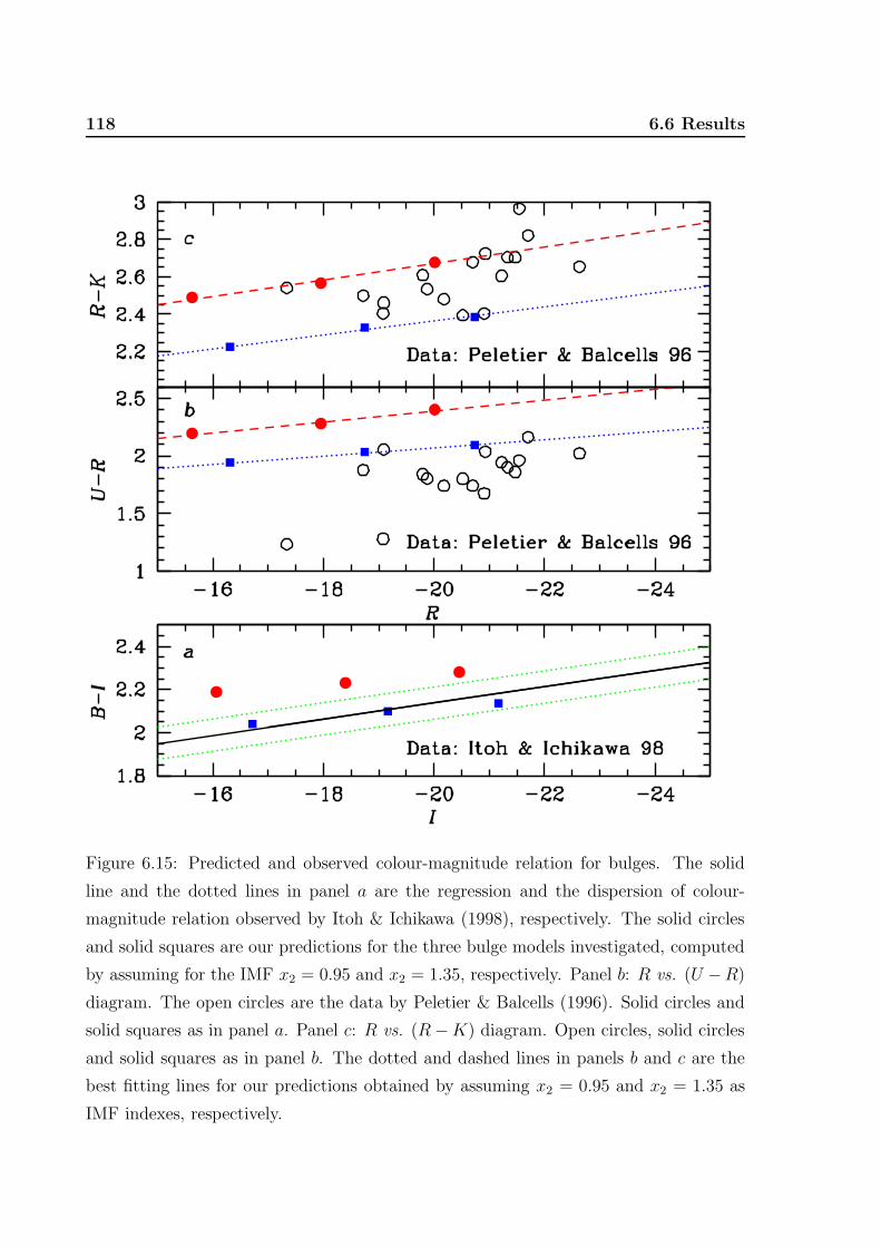
118 6.6 Results
Figure 6.15: Predicted and observed colour-magnitude relation for bulges. The solid
line and the dotted lines in panel a are the regression and the dispersion of colour-
magnitude relation observed by Itoh & Ichikawa (1998), respectively. The solid circles
and solid squares are our predictions for the three bulge models investigated, computed
by assuming for the IMF x2 = 0.95 and x2 = 1.35, respectively. Panel b: R vs. (U −R)
diagram. The open circles are the data by Peletier & Balcells (1996). Solid circles and
solid squares as in panel a. Panel c: R vs. (R−K) diagram. Open circles, solid circles
and solid squares as in panel b. The dotted and dashed lines in panels b and c are the
best fitting lines for our predictions obtained by assuming x2 = 0.95 and x2 = 1.35 as
IMF indexes, respectively.

Chapter 6. Chemical evolution of Seyferts and bulge photometry 119
Photometric properties of the galactic bulges
(B − R) (U − R) (R − K)
Observed (a) 1.27 − 1.6 1.24 − 2.16 2.39 − 2.97
(b) 0.5 − 2.18
Predicted (x = 1.35) 1.64 − 1.71 1.94 − 2.09 2.22 − 2.38
(x = 0.95) 1.75 − 1.83 2.20 − 2.40 2.49 − 2.68
Table 6.3: Predicted colours for galactic bulges assuming two different IMFs, compared
to observational values of local bulges from various sources (a: Balcells & Peletier 1994;
b: Galaz et al. 2006.)
observations.
From the analysis of the R vs. (U − R) diagram, we note that our predictions
computed assuming x2 = 1.35 are consistent with the observations, in particular for the
bulge models of masses 2×10¹⁰M and 1011M. For the lowest-mass bulge, correspond-
ing to the highest absolute R magnitude, the (U −R) colour seems to be overestimated.
In Table 6.3, we present our results for the predicted present-day colours for the bulge
model of mass 2×10¹⁰M, computed for two different IMFs, compared to observational
values for local bulges derived by various authors. The present-day values are computed
at 13.7 Gyr. Note that, for each colour, the observational values represent the lowest and
highest observed values reported by the authors. The values we predict are compatible
with the observations of local bulges, which show a considerable spread. However, the
sample of bulges considered here seems to be skewed towards high-mass bulges, making
it difficult to infer the trend of the R vs. (U −R) for magnitudes R < −16 mag. On the
other hand, the predictions computed by assuming x2 = 0.95 seem to produce (U −R)
colours that are much too high with respect to the observations. Finally, the R vs.
(R−K) diagram does not allow us to draw any firm conclusion on the slope of the IMF.
From the combined study of the I vs. (B − I), R vs. (U − R) and R vs. (R −K)
diagrams, we conclude that the observational data for local bulges seem to disfavour
IMFs flatter than x2 = 1.35 in the stellar mass range 1 ≤ m/M ≤ 80. In Table 6.3,
we present our results for the predicted present-day colours for the three bulge models
presented, computed for two different IMFs. The present-day values are computed at
13.7 Gyr. Still in Table 6.3, we also show the observational data of Peletier & Balcells
(1996) and of Galaz et al. (2006), who estimate that dust effects should be small
120 6.7 Summary and conclusions
for their sample, with an upper limit on the extinction of 0.3 mag. For each colour,
the observational values again represent the lowest and highest values reported by the
authors.
For the model with mass comparable to the one of the bulge of the Milky Way
galaxy, i.e. the one with a total mass M = 2 × 10¹⁰M, with the assumption of an
IMF with x2 = 0.95, we predict a present K-band luminosity LBul,K = 4.5 × 10⁹L.
Existing observational estimates of the K-band luminosity of the bulge indicate values
0.96 × 10¹⁰ ≤ LBul,K,obs ≤ 1.8 × 10¹⁰L (Dwek et al. 1995, Launhardt et al. 2002), i.e.
at least a factor of 2 higher than the estimate obtained with our model. By adopting
an IMF with x2 = 1.35, we obtain Lx=1.35Bul,K = 7.6 × 10⁹L, in better agreement with the
observed range of values.
6.7 Summary and conclusions
We made use of our self-consistent model of galactic evolution which reproduces the
main observational features of the Galactic bulge (Ballero et al. 2007a) to study the
fuelling and the luminous output of the central supermassive black hole in spiral bulges,
as fed by the stellar mass loss and cosmological infall, at a rate given by the minimum
between the Eddington and Bondi accretion rates in order to make predictions about
the evolution of Seyfert nuclei. A realistic galaxy model was adopted to estimate the gas
binding energy in the bulge, and the combined effect of AGN and supernova feedback
was taken into account as contributing to the thermal energy of the interstellar medium.
We also investigated the chemical composition of the gas restored by stars to the inter-
stellar medium. Assuming that the gas emitting the broad and narrow lines observed in
Seyfert spectra is well mixed with the bulge interstellar medium, we have made specific
predictions regarding Seyfert metallicities and abundances of several chemical species
(Fe, O, Mg, Si, Ca, C and N), and their redshift evolution. Finally, we calculated the
evolution of the (B−K) and (U−B) colours, the present-day bulge colours and K-band
luminosity and the colour-magnitude relation, and discussed their dependence on the
adopted IMF.
Our main results can be summarised as follows:
1. The AGN goes through a first phase of Eddington-limited accretion and a second
phase of Bondi-limited accretion. Most of the fuelling (and of the shining) of
the AGN occurs at the transition between the two phases, which approximately

Chapter 6. Chemical evolution of Seyferts and bulge photometry 121
coincides with the occurrence of the wind. Within a factor of two, the final black
hole mass is reached in a fraction of the bulge lifetime ranging from 2 to 6%.
2. Since, like in Ballero et al. (2007a), the galactic wind occurs after the bulk of star
formation, it does not have considerable effects on the chemical abundances. It
only plays a part in regulating the final black hole mass.
3. The peak bolometric luminosities predicted for AGNs residing in the bulge of spiral
galaxies are in good agreement with those observed in Seyfert galaxies (' 1042 −1044 erg s−1). At late times, the model nuclear luminosities (produced by accretion
of the mass return from the passively ageing stellar populations) are < 1042 erg s−1,
and would be further reduced by a factor ∼ 0.01 when considering advection-
dominated accretion flow regimes or its variants. To recover an agreement with
the luminosities of local Seyferts, it is necessary to assume a rejuvenation event in
the past 1 − 2 Gyrs.
4. The feedback from the central AGN is not in any case the main one responsible
for triggering the galactic wind, since its contribution to the thermal energy is at
most comparable to that of the supernova feedback.
5. The proportionality between the mass of the host bulge and that of the central
black hole is reproduced very well without the need to switch off the accretion
ad hoc. We derived an approximate relation of MBH ≈ 0.0009Mb, consistent
with recent estimates (McLure & Dunlop 2002; Marconi & Hunt 2003; Haring &
Rix 2004).
6. The huge star formation rates (several thousands solar masses a year) needed
to produce the observed line strengths, dust content and metallicities of Seyfert
galaxies are easily attained. Due to such a high star formation rate, solar metal-
licity is reached in less than 108 yr, and solar abundances for the elements we
considered are reached in a few hundred million years. This naturally explains
the high metallicities and abundances inferred for Seyfert galaxies in analogy with
QSOs.
7. After the first ∼300 million years, the interstellar medium in the bulge reaches
overabundances of up to one order of magnitude for N, Fe, Si, Ca, up to 5 times
solar for Mg and 3 times solar for C and O. This is roughly consistent with the

122 6.7 Summary and conclusions
estimates for Fe, N and O in the broad and intrinsic narrow line regions of Seyfert
galaxies. The slightly supersolar [Fe/Mg] and its weak dependence on the galaxy
luminosity (mass) are recovered. These results remain essentially unchanged if we
adopt a Salpeter (1955) stellar IMF.
8. The mean value assumed by the [N/C] abundance ratio is very sensitive to the
galaxy mass, due to the sensitivity of N to metallicity. The calculated values are
consistent with recent estimates (Fields et al. 2005a).
9. Higher bulge masses imply redder colours, in agreement with the downsizing pic-
ture of galaxy evolution. A flatter IMF gives rise to a redder bulge. While the
present-day bulge colours are well fitted both by a top-heavy (x2 = 0.95) and a
Salpeter (x2 = 1.35) IMF, the latter is required in order to achieve a better agree-
ment with the colour-magnitude relation and the present-day K-band luminosity
of the bulge.

Chapter 7
Concluding remarks
”There was a point to this story, but it has temporarily escaped the chronicler’s mind.”
(Douglas Adams)
7.1 Summary
In this thesis, we undertook the task of updating the existing models of chemical evolu-
tion of the Galactic bulge, based on the most recent high-quality datasets of abundances
in bulge evolved stars, and to begin investigating the link between supermassive black
holes residing in spiral galaxies and the host galaxies themselves, in a framework where
bulges are old stellar systems formed by a fast collapse of gas at a very early epoch.
A variety of independent observables helped us carry out a consistent picture where
we derived information about the processes of galactic formation and evolution, stellar
nucleosynthesis and about the relative role played by supernova and black hole feedback.
The conclusions achieved in this investigation can be shortly summarised as follows:
• We confirm that a short formation timescale combined with a high star formation
efficiency (the value we suggest is 20 Gyr−1) fits the observed metallicity distri-
bution and naturally explain the α-enhancements detected in bulge stars up to
∼solar metallicities. The star formation history of the Galactic bulge can thus be
assimilated to that of an elliptical, with a strong burst of star formation at the
beginning which vanishes very soon thereafter. A finite, though small, accretion
time (of the order of 0.1 Gyr) prevents the formation of an excessive amount of
low-metallicity stars, although this phenomenon is much less serious than in the
solar neighbourhood (G-dwarf problem). Values of τ longer than 0.1 Gyr can

124 7.1 Summary
combine with values of ν lower than 20 Gyr−1 and match the observed metallicity
distribution. However, such a “degeneracy” is broken when we consider also the
evolution of [O/Fe] vs. [Fe/H].
• The observations of nitrogen in the giants and planetary nebulae of the bulge
cannot give us a strong constraint on the nucleosynthesis of nitrogen in massive
stars, since nitrogen in evolved stars is generally self-enriched. However, a primary
contribution of this element from massive stars seems to be required if we suppose
that the average trend of the [N/O] vs. [O/H] abundance ratio reflects the pristine
one. Clearly, measurements performed in less evolved environments would help
settle this point.
• Results concerning the stellar initial mass function (IMF) are contradictory. A
Scalo (1986) or Weidner & Kroupa (2005) IMF are robustly excluded by observa-
tions. Considerations on the metallicity distribution of giants in the Galactic bulge
and in the bulge of M31 seem to favour a rather flat IMF, with an index x ∼ 1
for masses above 1M, instead of a Salpeter (1955) index (x ' 1.35); in general, a
variation of the IMF among the various environment is suggested. The [α/Fe] vs.
[Fe/H] plots do not provide a strong constraint on this point. On the contrary, the
photometric features of local bulges (colour-magnitude relation, present K-band
luminosity) can only be reproduced by means of a Salpeter IMF. The specific pre-
dictions we have made represent a challenge to observe essential data in order to
test these predictions. We suggest to extend the photometric measurements to a
larger sample of bulges, and to carefully investigate the presence and effects of any
observational biases.
• Mass loss from massive stars and its effects on the chemical yields, which depend
on metallicity, provide a natural mechanism to solve the long-standing discrep-
ancy between the trend of [O/Fe] at high [Fe/H] and the other [α/Fe] trends in
the Galactic disk and bulge, and to significantly improve the agreement between
predicted and observed [O/Mg] ratios in the bulge and disk above solar metallicity.
A small zero-point normalisation problem remains, which could imply either that
the yields of Francois et al. (2004) need adjustment, or that the bulge IMF is
steeper than the reference one (x = 0.95). The former explanation is preferred,
since preliminary results obtained with a Salpeter (1955) IMF show that the slope
of [O/Mg] for supersolar metallicities is poorly reproduced. A combination of the

Chapter 7. Concluding remarks 125
two factors may explain this offset as well.
• Simple recipes for black hole accretion and feedback, based on Eddington-limited
accretion, can account for the peak bolometric luminosity and for the observed
relation between bulge mass and black hole mass in Seyfert galaxies. The radiative
feedback from the black hole is not important in the energy budget, since it is at
most comparable to the supernova feedback. Taking into account the Bondi rate
allows to reproduce the final black hole masses without forcing the accretion phase
to stop at a determined time. However, the predicted bolometric luminosities of
local Seyfert nuclei hosted by bulges with M < 1011M fall below the observations
by about the same factor. Therefore, these bulges must experience a secondary
accretion episode at low (z < 1) redshift turning 10−30% of their mass into stars,
as also suggested by other independent observations.
• The occurrence of the galactic wind is of secondary importance in determining
the chemical properties of both active and inactive bulges, since it occurs after
the bulk of gas has already been turned into stars; it only helps reproduce the
high-metallicity tail in the [Fe/H] distribution. Since the Bondi accretion rate
depends on the gas density, its sharp decrease induced by the one-step wind may
play some part in determining the exact final black hole mass in Seyferts; however
since the gas consumption in the bulge is very fast, we expect that the adoption
of a continuous wind would not change the results significantly.
• The chemical properties of Seyfert galaxies and AGN in general, such as the high
metallicities and the constancy of chemical abundances up to very high redshifts
(z ∼ 6 − 7), as well as the huge star formation rates inferred from line strengths,
dust content and metallicities, are consistent with a star formation history typical
of old bulges, where a strong major episode of star formation occurs in the first few
hundred million years of bulge lifetime and then gets switched off quickly. The
underlying model for the Galactic bulge also explains fairly well the overabun-
dances of certain elements (Fe, N, O) observed in the broad and intrinsic narrow
line regions of Seyfert galaxies.

126 7.2 Future perspectives
7.2 Future perspectives
We briefly outline some of the future investigations which may be carried out as a natural
consequence of the work presented in this thesis:
1. As stated in Chapter 3, carbon and nitrogen in evolved stars are likely to be self-
processed, so that the abundances of these elements measured in giants are not in
general the pristine ones. In particular, carbon is consumed to form nitrogen. It
is thus probable that the (C+N) abundance is less affected by stellar evolution.
A study of the evolution of the [C+N/Fe] abundance ratio with metallicity is
underway and confirms that a certain amount of primary nitrogen from massive
stars is necessary.
2. The inclusion of sodium and aluminium nucleosynthesis in chemical evolution mod-
els will allow the comparison with the most recent measurements of these two
elementary abundances in the solar neighbourhood and Galactic bulge.
3. The oxygen yields of Meynet & Maeder (2000, 2002) and Hirschi (2007), which take
rotation and mass loss into account, should be tested in the solar neighbourhood
and bulge to see if they can reproduce the [O/Fe] and [O/Mg] trends as discussed
in Chapter 4.
4. The effects of primordial nucleosynthesis from zero-metal stars (Population III
stars) on the chemical evolution of the bulge can be investigated.
5. The spectral energy distribution of an accreting supermassive black hole and of a
dusty torus can be calculated so that predictions about the spectro-photometric
properties of actual Seyfert 1 and Seyfert 2 galaxies can be made.
6. The calculations carried here for the black hole feedback can be integrated into
multi-zone models for elliptical galaxies, so that the chemical evolution of QSOs
hosted by ellipticals can be studied.

Appendix A
The disk gravitational energy
contributions
In Chapter 6, we assumed spherical symmetry for the bulge gas distribution in order
to estimate the binding energy of the gas itself. Thus, the contribute of the spherical
stellar bulge and the spherical dark matter halo are given by the elementary expressions
in Eqs. 6.13 and 6.14.
A more complicate case is represented by the disk-gas interaction. In fact, one could
suppose that a two-dimensional integral, involving special functions must be evaluated,
because of the disk geometry. However, this is not the case: in fact, if each gas element
is displaced radially from r to rt, then
∆Egd =
∫ rt
0
ρg(r)r2dr
∫
4π
dΩ[φd(errt) − φd(err)] =
= 4π
∫ rt
0
ρg(r)r2[φd(rt) − φd(r)]dr (A.1)
where
φd(r) =1
4π
∫
4π
φd(err)dΩ (A.2)
is the angular averaged potential, and er the radial unit vector. It is trivial to prove by
direct evaluation that the angular mean of the potential of a generic density distribution
is also the (spherical) potential of the angular averaged density. Of course, this result
can also be obtained in a more elegant way by considering the angular mean of the
expansion of the potential in spherical harmonics (e.g., Binney & Tremaine 1987), so
that all the terms vanish, except the monopole. An identical argument also holds in the

128
case of the computation of the virial trace. In fact, from x = err it follows that
Wbd = −∫ρg < x,∇φd > d3x = −4π
∫ρg(r)
dφd(r)
drr3dr. (A.3)
The surface density of a razor-thin axisymmetric disk in spherical coordinates is
Σ(r, ϑ, ϕ) =Σd(r sinϑ)δ(cos ϑ)
r, (A.4)
so that
ρd(r) =1
4π
∫
4π
Σ(r, ϑ, ϕ)dΩ =Σd(r)
2r(A.5)
For the exponential disk in Eq. 6.10 we then obtain
φd(r) = −GMd
r
(1 − e−r/Rd
), (A.6)
so that integrations in Eqs. A.1 and A.3 reduce to
∆Egd =δ + (1 − h)(1 − e−δ/h)
1 + δ+
+e1/h
h
[Ei
(−1
h
)− Ei
(−1
h− 1
δ
)](A.7)
and
Wbd = −1
h− e1/h(1 + h)
h2Ei
(−1
h
)(A.8)
where h ≡ Rd/rb, δ ≡ rt/rb, and Ei(−x) = −∫∞
re−tt−1dt is the exponential integral.

Bibliography
[1] Adams, T.F., 1977, ApJS 33, 19
[2] Aguerri, J.A.L., Balcells, M., Peletier, R.F., 2001, A&A 373, 786
[3] Alard, C., 1996, PhD thesis, University of Paris VI
[4] Angeletti, L., Giannone, P., 1990, A&A 234, 53
[5] Antonucci, R., 1993, ARA&A 31, 473
[6] Arimoto, N., Yoshii, Y., 1986, A&A 164, 260
[7] Arimoto, N., Yoshii, Y, 1987, A&A 173, 23
[8] Arnett, D., 1991, in “Frontiers of Stellar Evolution”, ed. D.L. Lambert, ASP Conf.
Series 20, 389
[9] Asplund, M., Grevesse, N., Sauval, A.J., 2005, in “Cosmic Abundances as Records
of Stellar Evolution and Nucleosynthesis”, eds. Thomas G. Barnes III & Frank N.
Bash, ASP Conf. Series 336, 25
[10] Balcells, M., Peletier, R.F., 1994, AJ 107, 135
[11] Baldwin, J.A., Ferland, G.J., Korista, K.T., Hamann, F., LaCluyze, A., 2004, ApJ
615, 610
[12] Ballero, S.K., Kroupa, P., Matteucci, F., 2007b, A&A 467, 117
[13] Ballero, S.K., Matteucci, F., Chiappini, C., 2006, NewA 11, 306
[14] Ballero, S.K., Matteucci, F., Ciotti, L., Calura, F., Padovani, P., 2008, A&A, in
press (arXiv:0710.4129 )
[15] Ballero, S.K., Matteucci, F., Origlia, L., Rich, R.M., 2007a, A&A 467, 124

130 BIBLIOGRAPHY
[16] Barbuy, B., 1999, Ap&SS 265, 319
[17] Barth, A.J., Martini, P., Nelson, C.H., Ho, L.C., 2003, ApJ 594, L95
[18] Baugh, C.M., Lacey, C.G., Frenk, C.S., Granato, G.L., Silva, L., Bressan, A.,
Benson, A.J., Cole, S., 2005, MNRAS 356, 1191
[19] Baumgardt, H., Makino, J., 2003, MNRAS 340, 227
[20] Bender, R., Burstein, D., Faber, S.M., 1992, ApJ 399, 462
[21] Bensby, T., Feltzing, S., Lundstrom, I., 2004, A&A 415, 155
[22] Bensby, T., Feltzing, S., Lundstrom, I., Ilyn, I., 2005, A&A 433, 185
[23] Bentz, M.C., Hall, P.B., Osmer, P.S., 2004, AJ 128, 561
[24] Bertin, G., Saglia, R.P., Stiavelli, M., 1992, ApJ 384, 423
[25] Bertola, F., Vietri, M., Zeilinger, W.W., 1991, ApJ 374, L13
[26] Binney, J., Tremaine, S., 1987, “Galactic Dynamics”, Princeton University Press,
Princeton, NJ
[27] Blain, A.W., Smail, I., Ivison, R.J., Kneib, J.P., Frayer, D.T., 2002, Physic Reports
369, 111
[28] Bondi, H., 1952, MNRAS 112, 195
[29] Brandt, W.N., Hasinger, G., 2005, ARA&A 43, 827
[30] Bromm, V., Larson, R.B., 2004, ARA&A 42, 79
[31] Brown, J.A., Wallerstein, G., Zucker, D., 1997, AJ 114, 180
[32] Burstein D., Bender, R., Faber, S.M., Nolthenius, R., 1997, AJ 114, 1365
[33] Calura, F., Jimenez, R., Panter, B., Matteucci, F., Heavens, A. F., 2007a, MNRAS
submitted (arXiv:0707.1345v2 )
[34] Calura, F., Matteucci, F., 2003, ApJ 596, 734
[35] Calura, F., Matteucci, F., 2006, ApJ 652, 889

BIBLIOGRAPHY 131
[36] Calura, F., Matteucci, F., Menci, N., 2004, MNRAS 353, 500
[37] Calura, F., Matteucci, F., Tozzi, P., 2007b, MNRAS 378, L11
[38] Calura, F., Pipino, A., Matteucci, F., 2007c, A&A accepted (arXiv:0706.2197v1 )
[39] Carretta, E., Cohen, J., Gratton, R.G., Behr, B. 2001, AJ, 122, 1469
[40] Castro, S., Rich, R.M., Grenon, M., Barbuy, B., McCarthy, J.K., 1997, AJ 114, 376
[41] Cavaliere, A., Vittorini, V., 1998, in “The Young Universe: Galaxy Formation and
Evolution at Intermediate and High Redshift”, eds. S. D’Odorico, A. Fontana & E.
Giallongo, ASP Conf. Series 146, 26
[42] Chabrier, G., 2003, PASP 115, Issue 809, 763
[43] Chiappini, C., Hirschi, R., Meynet, G., Elstrom, S., Maeder, A., Matteucci, F.,
2006, A&A 449, L27
[44] Chiappini, C., Matteucci, F., Ballero, S.K., 2005, A&A 437, 429
[45] Chiappini, C., Matteucci, F., Gratton, R., 1997, ApJ 477, 765
[46] Chiappini, C., Matteucci, F., Meynet, G., 2003a, A&A 410, 257
[47] Chiappini, C., Matteucci, F., Romano, D., 2003b, ApJ 554, 1044
[48] Chiappini, C., Romano, D., Matteucci, F., 2003c, MNRAS 339, 63
[49] Cimatti, A., Pozzetti. L., Mignoli, M., Daddi, E., Menci, N., Poli, F., Fontana, A.,
Renzini, A., Zamorani, G., Broadhurst, T., Cristiani, S., D’Odorico, S., Giallongo,
E., Gilmozzi, R., 2002, A&A 391, L1
[50] Cioffi, D.F., McKee, C.F., Bertschinger, E., 1988, ApJ 334, 252
[51] Ciotti, L., Ostriker, J.P., 1997, ApJ 487, L105
[52] Ciotti, L., Ostriker, J.P., 2001, ApJ 551, 131
[53] Ciotti, L., Ostriker, J.P., 2007, ApJ 665, 1038
[54] Collin, S., Joly, M., 2000, NewAR 44, 531
[55] Combes, F., Sanders, R.H., 1981, A&A 96, 164

132 BIBLIOGRAPHY
[56] Costa, R.D.D., Escudero, A.V., Maciel, W.J., 2005, in “Planetary Nebulae as As-
tronomical Tools”, AIP Conference Proceedings, Volume 804, p. 252
[57] Cox, D.P., 1972, ApJ 178, 143
[58] Cox, P., Omont, A., Djorgovski, S.G., Bertoldi, F., Pety, J., Carilli, C.L., Isaak,
K.G., Beelen, A., McMahon, R.G., Castro, S., 2002, A&A 387, 406
[59] Cuisinier, F., Maciel., W.J., Koppen, J., Acker, A., Stenholm, B., 2000, A&A
353, 543
[60] Dietrich, M., Hamann, F., Appenzeller, I., Vestergaard, M., 2003a, ApJ 596, 817
[61] Dietrich, M., Hamann, F., Shields, J.C., Constantin, A., Heidt, J., Jager, K., Vester-
gaard, M., Wagner, S.J., 2003b, ApJ 589, 722
[62] Di Matteo, T., Croft, R.A.C., Springel, V., Hernquist, L., 2003, ApJ 593, 56
[63] Di Matteo, T., Springel, V., Hernquist, L., 2005, Nature 433, 604
[64] Djorgovski, S., Davis, M., 1987, ApJ 313, 59
[65] D’Odorico, V., Cristiani, S., Romano, D., Granato, G.L., Danese, L., 2004, MNRAS
351, 976
[66] Dopita, M.A., Ryder, S.D., 1994, ApJ 430, 163
[67] Dunlop, J.S., McLure, R.J., Kukula, M.J., Baum, S.A., O’Dea, C.P., Hughes, D.H.,
2003, MNRAS 340, 1095
[68] Dwek, E., Arendt, R.G., Hauser, M.G., Kelsall, T., Lisse, C.M., Moseley, S.H.,
Silverberg, R.F., Sodroski, T.J., Weiland, J.L., 1995, ApJ 445, 716
[69] Edvardsson, B., Andersen, J., Gustafsson, B., Lambert, D. L., Nissen, P. E.,
Tomkin, J., 1993, A&AS 102, 603
[70] Eggen, O.J., Lynden-Bell, D., Sandage, A.R., 1962, ApJ 136, 748
[71] Elmegreen, B., 1999, ApJ 517, 103
[72] Escudero, A.V., Costa, R.D.D., 2001, A&A 380, 300
[73] Escudero, A.V., Costa, R.D.D., Maciel, W.J., 2004, A&A 414, 211

BIBLIOGRAPHY 133
[74] Fabian, A.C., Iwasawa, K., 2000, AdSpR 25, 471
[75] Falcon-Barroso, J., Peletier, R.F., Balcells, M., 2002, MNRAS 335, 741
[76] Feltzing, S., Gustafsson, B., 1998, A&AS 129, 237
[77] Ferrarese, L., Merritt, D., 2000, ApJ 539, L9
[78] Ferrarese, L., Pogge, R.W., Peterson, B.M., Merritt, D., Wandel, A., Joseph, C.L.,
2001, ApJ 555, L79
[79] Ferreras, I., Wyse, R.F.G., Silk, J., 2003, MNRAS 345, 1381
[80] Fields, D.L., Mathur, S., Pogge, R.W., Nicastro, F., Komossa, S., 2005a, ApJ
620, 183
[81] Fields, D.L., Mathur, S., Pogge, R.W., Nicastro, F., Komossa, S., Krongold, Y.,
2005b, ApJ 634, 928
[82] Figer, D.F., 2005, Nature 434, 192
[83] Figer, D.F., Kim, S.S., Morris, M., Serabyn, E., Rich, R.M., McLean, I.S., 1999,
ApJ 525, 750
[84] Ford, H.C., Tsvetanov, Z.I., Ferrarese, L., Jaffe, W., 1998, in “The Central Regions
of the Galaxy and galaxies”, ed. Y. Sofue, IAU Symp. 184, 377
[85] Fraquelli, H.A., Storchi-Bergmann, T., 2003, BASBr 23, 150
[86] Freudling, W., Corbin, M.R., Korista, K.T., 2003, ApJ 587, L67
[87] Francois , P., Matteucci, F., Cayrel, R., Spite, M., Spite, F., Chiappini, C., 2004,
A&A 421, 613
[88] Friaca, A.C.S., Terlevich, R.J., 1998, MNRAS 298, 399
[89] Friedli, D., Benz, W., 1993, A&A 268, 65
[90] Friedli, D., Benz, W., 1995, A&A 301, 649
[91] Fryer, C.L., Young, P.A., Hungerford, A.L., 2006, ApJ 650, 1028
[92] Fulbright, J.P., McWilliam, A., Rich, R.M., 2006, ApJ 636, 821

134 BIBLIOGRAPHY
[93] Fulbright, J.P., McWilliam, A., Rich, R.M., 2007, ApJ 661, 1152
[94] Galaz, G., Villalobos, A., Infante, L., Donzelli, C., 2006, AJ 131, 2035
[95] Gebhardt, K., Bender, R., Bower, G., Dressler, A., Faber, S.M., Filippenko, A.V.,
Green, R., Grillmair, C., Ho, L.C., Kormendy, J., Lauer, T., Magorrian, J., Pinkney,
J., Richstone, D., Tremaine, S., 2000a, ApJ 539, L13
[96] Gebhardt, K., Kormendy, J., Ho, L.C., Bender, R., Bower, G., Dressler, A., Faber,
S.M., Filippenko, A.V., Green, R., Grillmair, C., Lauer, T., Magorrian, J., Pinkney,
J., Richstone, D., Tremaine, S., 2000b, ApJ 543, L5
[97] Geisler, D., Smith, V.V., Wallerstein, G., Gonzalez, G., Charbonnel, C., 2005, AJ
129, 1428
[98] Genzel, R., Baker, A.J., Tacconi, L.J., Lutz, D., Cox, P., Guilloteau, S., Omont,
A., 2003, ApJ 584, 633
[99] Gonzalez Delgado, R.M., Heckman, T., Leitherer, C., Meurer, G., Krolik, J., Wil-
son, A.S., Kinney, A., Koratkar, A., 1998, ApJ 505, 174
[100] Gorny, S. K., Stasinska, G., Escudero, A. V., Costa, R. D. D., 2004, A&A 427,
231
[101] Granato, G.L., De Zotti, G., Silva, L., Bressan, A., Danese, L., 2004, ApJ 600, 580
[102] Greggio, L., Renzini, A., 1983, A&A 118, 217
[103] Grevesse, N., Sauval, A.J., 1998, SSRv 85, 161
[104] Groenewegen, M.A.T., Blommaert, J.A.D.L., 2005, A&A 443, 143
[105] Gu, Q., Melnick, J., Cid Fernandes, R., Kunth, D., Terlevich, E., Terlevich, R.,
2006, MNRAS 366, 480
[106] Haehnelt, M.G., Natarajan, P., Rees, M.J., 1998, MNRAS 300, 817
[107] Haiman, Z., Ciotti, L., Ostriker, J.P., 2004, ApJ 606, 763
[108] Hamann, F., Dietrich, M., Sabra, B.M., Warner, C., 2004, in “Origin and Evo-
lution of the Elements”, eds. A. McWilliam & M. Rauch, Carnegie Observatories
Astrophysics Series 4, 443

BIBLIOGRAPHY 135
[109] Hamann, F., Dietrich, M., Sabra, B., Warner, C., Barlow, T., Chaffee, F.,
Junkkarinen, V., 2003, in “CNO in the Universe”, eds. C. Charbonnel, D. Schaerer
& G. Meynet, ASP Conf. Series 304, 236
[110] Hamann, F., Ferland, G., 1993, ApJ 418, 11
[111] Hamann, F., Ferland, G., 1999, ARA&A 37, 487
[112] Hamann, F., Korista, K.T., Ferland, G.J., Warner, C., Baldwin, J., 2002, ApJ
564, 592
[113] Haring, N., Rix, H.W., 2004, ApJ 604, L89
[114] Harmon, R., Gilmore, G., 1988, MNRAS 235, 1025
[115] Hasan, H., Pfenniger, D., Norman, C., 1993, ApJ 409, 91
[116] Hernquist, L., 1990, ApJ 356, 359
[117] Hill, V., 1997, A&A 324, 435
[118] Hirschi, R., 2007, A&A 461, 571
[119] Ho, L.C., 1999, ApJ 516, 672
[120] Ho, L.C., Filippenko, A.V., Sargent, W.L.W., 1997, ApJ 487, 568
[121] Holtzman, J.A., Light, R.M., Baum, W.A., Worthey, G., Faber, S.M., Hunter,
D.A., O’Neil Jr., E.J., Kreidl, T.J., Groth, E.J., Westphal, J.A., 1993, AJ 106, 1826
[122] Hou, J., Chang, R., Fu C., 1998, Annals of Shanghai Observatory, Academia Sinica
No. 19, 96
[123] Ibata, R.A., Gilmore, G.F., 1995, MNRAS 275, 591
[124] Immeli, A., Samland, M., Gerhard, O., Westera, P., 2004, A&A 413, 547
[125] Itoh, N., Ichikawa, T., 1998, IAU Symp. 184, 55
[126] Ivanov, V.D., Alonso-Herrero, A., Rieke, M.J., 2003, in “Star Formation through
Time”, eds. E. Perez, R.M. Gonzalez Delgado, G. Tenorio-Tagle, ASP Conf. Series
297, 165

136 BIBLIOGRAPHY
[127] Iwamoto, K., Brachwitz, F., Nomoto, K., Kishimoto, N., Umeda, H., Hix, W.R.,
Thielemann, F.K., 1999, ApJS 125, 439
[128] Iwamuro, F., Kimura, M., Eto, S., Maihara, T., Motohara, K., Yoshii, Y., Doi,
M., 2004, ApJ 614, 69
[129] Iwamuro, F., Motohara, K., Maihara, T., Kimura, M., Yoshii, Y., Doi, M., 2002,
ApJ 565, 63
[130] Jiang, L., Fan, X., Vestergaard, M., Kurk, J.D., Walter, F., Kelly, B.C., Strauss,
M.A., 2007, AJ 134, 1150
[131] Jimenez, R., MacDonald, J., Dunlop, J.S., Padoan, P., Peacock, J.A., 2004,
MNRAS 349, 240
[132] Jimenez, R., Padoan, P., Matteucci, F., Heavens, A.F., 1998, MNRAS 299, 123
[133] Kaspi, S., Smith, P.S., Netzer, H., Maoz, D., Jannuzi, B.T., Giveon, U., 2000, ApJ
533, 631
[134] Kauffmann, G., 1996, MNRAS 281, 487
[135] Kennicutt Jr., R.C., 1998, ApJ 498, 541
[136] Kim, S.S., Figer, D.F., Kudritzki, R.P., Najarro, F., 2006, ApJ 653, L113
[137] Kobayashi, C., Umeda, H., Nomoto, K., Tominaga, N., Ohkubo, T., 2006, ApJ
653, 1145
[138] Kodama, T., 1997, PhD thesis, Institute of Astronomy, University of Tokyo
[139] Koen, C., 2006, MNRAS 365, 590
[140] Komossa, S., Mathur, S., 2001, A&A 374, 914
[141] Korista, K., Kodituwakku, N., Corbin, M., Freudling, W., 2004, in “AGN Physics
with the SDSS”, eds. G.T. Richards & P.B. Hall, ASP Conf. Series 311, 415
[142] Kormendy, J., 1982, ApJ 256, 460
[143] Kormendy, J., Kennicutt, Jr., R.C., 2004, ARA&A 42, 603
[144] Kormendy, J., Richstone, D., 1995, ARA&A 33, 581

BIBLIOGRAPHY 137
[145] Kroupa, P., 2001, MNRAS 332, 231
[146] Kroupa, P., Tout, C.A., Gilmore, G. 1993, MNRAS, 262, 545
[147] Kroupa, P., Weidner, C., 2003, ApJ 598, 1076
[148] Kuijken, K., Rich, R.M., 2002, AJ 124, 2054
[149] Kurk, J.D., Walter, F., Fan, X., Jiang, L., Riechers, D.A., Rix, H.W., Pentericci,
L., Strauss, M.A., Carilli, C., Wagner, S., 2007, ApJ, in press (arXiv:0707.1662 )
[150] Kurucz, R.L., 1992, IAU Symp. 149, 225
[151] Lanfranchi, G.A., Matteucci, F., 2004, MNRAS 351, 1338
[152] Langer, N., Henkel, C., 1995, Space Science Rev. 74, 343
[153] Laor, A., 2001, ApJ 553, 677
[154] Larson, R.B., 1998, MNRAS 301, 569
[155] Launhardt, R., Zylka, R., Mezger, P.G, 2002, A&A 384, 112
[156] Lecureur, A., Hill, V., Zoccali, M., Barbuy, B., Gomez, A., Minniti, D., Ortolani,
S., Renzini, A., 2007, A&A 465, 799
[157] Lee, Y.W., 1992, AJ 104, 1780
[158] Lee, J.C., Fabian, A.C., Brandt, W.N., Reynolds, C.S., Iwasawa, K., 1999,
MNRAS 310, 973
[159] Limongi, M., Chieffi, A., 2003, ApJ 592, 404
[160] Liu, X.W., Luo, S.G., Barlow, M.J., Danziger, I.J., Storey, P.J., 2001, MNRAS
327, 141
[161] Lucy, L.B., Solomon, P.M., 1970 ApJ 159, 879
[162] Luna, G.J.M., Costa, R.D.D., 2005, A&A 435, 1087
[163] MacKenty, J.W., 1990, ApJS 72, 231
[164] Maeder, A., 1992, A&A 264, 105

138 BIBLIOGRAPHY
[165] Maeder, A., Meynet, G. 1989, A&A, 210, 155
[166] Magorrian, J., Tremaine, S., Richstone, D., Bender, R., Bower, G., Dressler, A.,
Faber, S.M., Gebhardt, K., Green, R., Grillmair, C., Kormendy, J., Lauer, T.R.,
1998, AJ 115, 2285
[167] Maiolino, R., Cox, P., Caselli, P., Beelen, A., Bertoldi, F., Kaufman, M.J., Nagao,
T., Omont, A., Weiß, A., Walmsley, M., 2005, A&A 440, L51
[168] Maiolino, R., Juarez, Y., Mujica, R., Nagar, N.M., Oliva, E., 2003, ApJ 596, L155
[169] Mannucci, F., Della Valle, M., Panagia, N., Cappellaro, E., Cresci, G., Maiolino,
R., Petrosian, A., Turatto, M., 2005, A&A 433, 807
[170] Maraston, C., Greggio, L., Renzini, A., Ortolani, S., Saglia, R.P., Puzia, T.H.,
Kissler-Patig, M., 2003, A&A 400, 823
[171] Marconi, A., Hunt, L., 2003, ApJ 589, 21
[172] Markowitz, A., Edelson, R., Vaughan, S., Uttley, P., George, I.M., Griffiths, R.E.,
Kaspi, S., Lawrence, A., McHardy, I., Nandra, K., Pounds, K., Reeves, J., Schurch,
N., Warwick, R., 2003, ApJ 593, 96
[173] Massey, P., 1998, in “The Stellar Initial Mass Function”, eds. G. Gilmore & Debbie
Howell, ASP Conf. Series 142, 17
[174] Massey, P., 2003, ARA&A 41, 15
[175] Massey, P., Hunter, D.A., 1998, ApJ 493, 180
[176] Mathur, S., 2000, NewAR 22, 469
[177] Matteucci, F., 1986, MNRAS 221, 911
[178] Matteucci, F., 1992, ApJ 397, 32
[179] Matteucci, F., 1994, A&A 288, 57
[180] Matteucci, F., 2000, in “The Evolution of the Milky Way: Stars versus Clusters”,
eds. F. Matteucci & F. Giovannelli, ASSL vol. 255, Kluwer Academic Publishers, p. 3
[181] Matteucci, F., Brocato, E., 1990, ApJ 365, 539

BIBLIOGRAPHY 139
[182] Matteucci, F., Greggio, L., 1986, A&A 154, 279
[183] Matteucci, F., Padovani, P., 1993, ApJ 419, 485
[184] Matteucci, F., Recchi, S., 2001, ApJ 558, 351
[185] Matteucci, F., Romano, D., Molaro, P., 1999, A&A 341, 458, MRM99
[186] Matteucci, F., Tornambe, A., 1987, A&A 185, 51
[187] MacArthur, L.A., Ellis, R.S., Treu, T., U, V., Bundy, K., Moran, S., 2007, sub-
mitted to ApJ (arXiv:0711.0238 )
[188] McLure, R.J., Dunlop, J.S., 2002, MNRAS 331, 795
[189] McWilliam, A., Matteucci, F., Ballero, S.K., Rich, R.M., Fulbright, J.P., Cescutti,
G., 2008, ApJ accepted (arXiv:0708.4026 )
[190] McWilliam, A., Rich, R.M., 1994, ApJS 91, 749, MR94
[191] McWilliam, A., Rich, R.M., 2004, in “Origin and Evolution of the Elements”,
from the Carnegie Observatories Centennial Symposia, Carnegie Observatories As-
trophysics Series, eds. A. McWilliam & M. Rauch, p. 38
[192] McWilliam, A., Rich, R.M., Smecker-Hane, T.A., 2003, ApJ 592, L21
[193] McWilliam, A., Smecker-Hane, T.A., 2005, “Cosmic Abundances as Records of
Stellar Evolution and Nucleosynthesis in honor of David Lambert”, eds. Thomas G.
Barnes III & Frank N. Bash, ASP Conference Series 336, 221
[194] Melendez, J., Barbuy, B., Bica, E., Zoccali, M., Ortolani, S., Renzini, A., Hill, V.
2003, A&A, 411, 417
[195] Meynet, G., Maeder, A., 2002, A&A 390, 561
[196] Meynet, G., Maeder, A., 2003, A&A 404, 975
[197] Meynet, G., Maeder, A., 2005, A&A 429, 581
[198] Minniti, D., Olzsewski, E.W., Liebert, J., White, S.D.M., Hill, J.M., Irwin, M.J.,
1995, MNRAS 277, 1293

140 BIBLIOGRAPHY
[199] Minniti, D., Zoccali, M., 2007, to appear in “Formation and Evolution of
Galaxy Bulges”, eds. M. Bureau, E. Athanassoula & B. Barbuy, IAU Symp. 245
(arXiv:0710.3104 )
[200] Molla, M., Ferrini, F., Gozzi, G., 2000, MNRAS 316, 345
[201] Monaco, L., Bellazzini, M., Bonifacio, P., Buzzoni, A., Ferraro, F.R., Marconi, G.,
Sbordone, L., Zaggia, S., 2007, A&A 464, 201
[202] Monaco, P., Salucci, P., Danese, L., 2000, MNRAS 311, 279
[203] Nagao, T., Marconi, A., Maiolino, R., 2006, A&A 447, 157
[204] Nagao, T., Murayama, T., Shioya, Y., Taniguchi, Y., 2002, ApJ 575, 721
[205] Nagashima, M., Lacey, C.G., Baugh, C.M., Frenk, C.S., Cole, S., MNRAS
358, 1247
[206] Nakamura, F., Umemura, M., 2001, ApJ 548, 19
[207] Narayan, R., Yi, I. 1994, ApJ 428, L13
[208] Nelson, C.H., Green, R.F., Bower, G., Gebhardt, K., Weistrop, D., 2004, ApJ
615, 652
[209] Nissen, P.E., Schuster, W.J., 1997, A&A 326, 751
[210] Noguchi, M., 1999, ApJ 514, 77
[211] Nomoto, K., Thielemann, F.K., Yokoi, K., 1984, ApJ 286, 644
[212] Norman, C.A., Sellwood, J.A., Hasan, H., 1996, ApJ 462, 114
[213] Nugis, T., Lamers, H.J.G.L.N., 2000, A&A 360, 227
[214] Nussbaumer, H., Schmid, H.M., Vogel, M., Schild, H., 1988, A&A 198, 179
[215] Oey, M.S., Clarke, C.J., 2005, ApJ 620, L430
[216] Okamoto, T., Eke, V.R., Frenk, C.S., Jenkins, A., 2005, MNRAS 363, 1299
[217] Onken, C.A., Ferrarese, L., Merritt, D., Peterson, B.M., Pogge, R.W., Vester-
gaard, M., Wandel, A., 2004, ApJ 615, 645

BIBLIOGRAPHY 141
[218] Origlia, L., Ferraro, F.R., Bellazzini, M., Pancino, E., 2003, ApJ, 591, 916
[219] Origlia, L., Rich, R.M., 2004, AJ 127, 3422
[220] Origlia, L., Rich, R.M., Castro, S., 2002 AJ 123, 1559
[221] Origlia, L., Valenti, E., Rich, R.M., 2005, MNRAS 256, 127
[222] Ortolani, S., Renzini, A., Gilmozzi, R., Marconi, G., Barbuy, B., Bica, E., Rich,
R.M., 1995, Nature 377, 701
[223] Osmer, P.S., Shields, J.C., 1999, in “Quasars and Cosmology”, eds. G. Ferland &
J. Baldwin, ASP Conf. Series 162, 235
[224] Ostriker, J.P., Ciotti, L., 2005, Philosophical Transactions of the Royal Society
Part A, 363, 1828, 667
[225] Padoan, P., Nordlund, A., Jones, B.J.T., 1997, MNRAS 288, 145
[226] Padovani, P., Matteucci, F., 1993, ApJ 416, 26
[227] Paresce, F., de Marchi, G., 2000, ApJ 534, 870
[228] Paumard, T., Genzel, R., Martins, F., Nayakshin, S., Beloborodov, A.M., Levin,
Y., Trippe, S., Eisenhauer, F., Ott, T., Gillessen, S., Abuter, R., Cuadra, J., Alexan-
der, T., Sternberg, A., 2006, ApJ 643, 1011
[229] Peimbert, M., Serrano, A., 1980, RMxAA 5, 9
[230] Peletier, R.F., Balcells, M., 1996, AJ 111, 2238
[231] Peletier, R.F., Balcells, M., Davies, R.L., Andredakis, Y., Vazdekis, A., Burkert,
A., Prada, F., 1999, MNRAS 310, 703
[232] Peterson, B.M., 2003, in “Active Galactic Nuclei: from central engine to host
galaxy”, eds. S. Collin, F. Combes & I. Shlosman, ASP Conf. Series 290, 43
[233] Petitjean, P., Srianand, R., 1999, A&A 345, 73
[234] Pfenniger, D., Norman, C.A., 1990, ApJ 363, 391
[235] Piotto, G., Zoccali, M., 1999, A&A 345, 485
142 BIBLIOGRAPHY
[236] Pipino, A., D’Ercole, A., Matteucci, F., 2007a, submitted to A&A
(arXiv:0706.2932 )
[237] Pipino, A., Matteucci, F., Borgani, S., Biviano, A., 2002, NewA 7, 227
[238] Pipino, A., Matteucci, F., D’Ercole, A., 2007b, to appear in “Formation and
Evolution of Galaxy Bulges”, eds. M. Bureau, E. Athanassoula & B. Barbuy, IAU
Symp. 245 (arXiv:0709.0658 )
[239] Pompeia, L., Barbuy, B., Grenon, M., 2003, ApJ 592, 1173
[240] Prantzos, N., Aubert, O., Audouze, J., 1996, A&A 309, 760
[241] Ramırez, S.V., Stephens, A.W., Frogel, J.A., DePoy, D.L., 2000, AJ 120, 833
[242] Reddy, B.E., Lambert, D.L., Allende Prieto, C., 2006, MNRAS 367, 1329
[243] Renzini, A., 1993, in “Galactic Bulges”, IAU Symp. 153, eds. H. DeJonghe & H.J.
Habing (Kluwer Academic Publishers, Dordrecht), 151
[244] Renzini, A., 1999, Ap&SS 267, 357
[245] Renzini, A., Voli, M., 1981, A&A 94, 175
[246] Rich, R.M., 1988, AJ 95, 828
[247] Rich, R.M., Origlia, L., 2005, ApJ 634, 1293
[248] Rodrıguez-Ardila, A., Contini, M., Viegas, S.M., 2005, MNRAS 357, 220
[249] Romano, D., Silva, L., Matteucci, F., Danese, L., 2002, MNRAS 334, 444
[250] Sadler, E.M., Rich, R.M., Terndrup, D.M., 1996, AJ 112, 171
[251] Salaris, M., Weiss, A., Percival, S.M., 2004, A&A 414, 163
[252] Salpeter, E.E., 1955, ApJ 121, 161
[253] Salpeter, E.E., 1964, ApJ 140, 796
[254] Samland, M., Hensler, G., Theis, C., 1997, ApJ 476, 544
[255] Sarajedini, A., Jablonka, P., 2005, AJ 130, 1627

BIBLIOGRAPHY 143
[256] Sarzi, M., Shields, J.C., Pogge, R.W., Martini, P., 2007, to appear in “Stellar
Populations as Building Blocks of Galaxies”, IAU Symp. 241, eds. R.F. Peletier & A.
Vazdekis (arXiv:astro-ph/0703794 )
[257] Sazonov, S.Y., Ostriker, J.P., Ciotti, L., Sunyaev, R.A., 2005, MNRAS 358, 168
[258] Scalo, J., 1986, FCPh 11, 1
[259] Scannapieco, E., Silk, J., Bouwens, R., 2005, ApJ 635, L13
[260] Schaerer, D., 2002, A&A 382, 28
[261] Schmidt, M., 1959, ApJ 129, 243
[262] Schmidt, M., Green, R.F., 1983, ApJ 269, 352
[263] Schmitt, H.R., Storchi-Bergmann, T., Baldwin, J.A., 1994, ApJ 423, 237
[264] Schwarzschild, M., Harm, R., 1959, ApJ 129, 637
[265] Schweizer, F., Seitzer, P., 1988, ApJ 328, 88
[266] Searle, L., Zinn, R., 1978, ApJ 225, 357
[267] Seyfert, C.K., 1943, ApJ 97, 28
[268] Shetrone, M.D., Cote, P., Sargent, W.L.W., 2001, ApJ 548, 592
[269] Shields, G.A., Gebhardt, K., Salviander, S., Wills, B.J., Xie, B., Brotherton, M.S.,
Yuan, J., Dietrich, M., 2003, ApJ 583, 124
[270] Stasinska, G., Tylenda, R., Acker, A., Stenholm, B., 1991, A&A 247, 173
[271] Storchi-Bergmann, T., 1991, MNRAS 249, 404
[272] Storchi-Bergmann, T., Bica, E., Pastoriza, M.G., 1990, MNRAS 245, 749
[273] Storchi-Bergmann, T., Pastoriza, M.G., 1989, ApJ 347, 195
[274] Storchi-Bergmann, T., Wilson, A.S., Baldwin, J.A., 1996, ApJ 460, 252
[275] Terndrup, D.M., 1988, AJ 96, 884

144 BIBLIOGRAPHY
[276] Thielemann, F.K., Nomoto, K., Hashimoto, M., 1993, in “Origin and Evolution of
the Elements”, eds. N. Prantzos, E. Vangioni-Flam & M. Casse, Cambridge University
Press, Cambridge, p. 297
[277] Thomas, D., Davies, R.L., 2006, MNRAS 366, 510
[278] Thomas, D., Greggio, L. Bender, R., 1998, MNRAS 296, 119
[279] Thomas, D., Maraston, C., Bender, R., 2002, Ap&SS, 281, 371
[280] Thompson, K.L., Hill, G.J., Elston, R., 1999, ApJ 515, 487
[281] Tinsley, B.M., 1979, ApJ 229, 1046
[282] Tinsley, B.M., 1980, FCPh 5, 287
[283] Tolstoy, E., Venn, K.A., Shetrone, M.D., Primas, F., Hill, V., Kaufer, A., Thomas,
S., 2003, AJ 125, 707
[284] Tosi M., Steigman G., Matteucci F., Chiappini C., 1998, ApJ 498, 226
[285] Tremaine, S., Gebhardt, K., Bender, R., Bower, G., Dressler, A., Faber, S.M.,
Filippenko, A.M., Green, R., Grillmair, C., Ho, L.C., Kormendy, J., Lauer, T.R.,
Magorrian, J., Pinkey, J., Richstone, D., 2002, ApJ 574, 740
[286] Tsujimoto, T., Nomoto, K., Yoshii, Y., Hashimoto, M., Yanagida, S., Thielemann,
F.K., 1995, MNRAS 277, 945
[287] Turner, T.J., George, I., Netzer, H., 1999, ApJ 526, 52
[288] Ulrich, M.H., Comastri, A., Komossa, S., Crane, P., 1999, A&A 350, 816
[289] Van den Hoek, L.B., Groenewegen, M.A.T., 1997, A&AS 123, 305
[290] Van Loon, J.T., Gilmore, G.F., Omont, A., Blommaert, J.A.D.L., Glass, I.S.,
Messineo, M., Schuller, F., Schultheis, M., Yamamura, I., Zhao, H.S, 2003, MNRAS
338, 857
[291] Venn, K.,A., Irwin, M., Shetrone, M.D., Tout, C.A., Hill, V., Tolstoy, E., 2004,
AJ 128, 1177
[292] Verner, E., Bruhweiler, F., Verner, D., Johansson, S., Gull, T., 2003, ApJ 592, L59

BIBLIOGRAPHY 145
[293] Vink, J.S., Koter, A., Lamers, H.J.G.L.M., 2000, A&A 362, 295
[294] Wainscoat, R.J., Freeman, K.C., Hyland, A.R., 1989, ApJ 337, 163
[295] Walton, N.A., Barlow, M.J., Clegg, R.E.S., 1993, in “Galactic Bulges”, IAU Symp.
153, eds. H. DeJonghe & H.J. Habing (Kluwer Academic Publishers, Dordrecht), 337
[296] Wandel, A., 1999, ApJ 519, L39
[297] Wandel, A., Peterson, B.M., Malkan, M.A., 1999, ApJ 526, 579
[298] Wang, R., Wu, X.B., 2005, ChJAA 5, 299
[299] Warner, C., Hamann, F., Dietrich, M., 2003, ApJ 596, 72
[300] Webster, B.L., 1984, ASAu Proceedings vol. 5, 535
[301] Weidner, C., Kroupa, P., 2004, MNRAS 348, 187
[302] Weidner, C., Kroupa, P., 2005, ApJ 625, 754
[303] Whitford, A.E., 1978, ApJ 226, 777
[304] Wills, B.J., Shang, Z., Yuan, J.M., 2000, NewAR 44, 511
[305] Woosley, S.E., Weaver, T.A., 1995, ApJS 101, 181
[306] Wu, X.B., Han, J.L., 2001, A&A 380, 31
[307] Wyse, R.F.G., 1998, MNRAS 293, 429
[308] Wyse, R.F.G., 1999, Ap&SS 267, 145
[309] Yee, H.K.C., 1983, ApJ 473, 713
[310] Yu, Q., Tremaine, S., 2002, MNRAS 335, 965
[311] Zoccali, M., Barbuy, B., Hill, V., Ortolani, S., Renzini, A., Bica, E., Momany, Y.,
Pasquini, L., Minniti, D., Rich, R.M. 2004, A&A, 423, 507
[312] Zoccali, M., Cassisi, S., Frogel, J.A., Gould, A., Ortolani, S., Renzini, A., Rich,
R.M., Stephens, A.W., 2000, ApJ 530, 418

146 BIBLIOGRAPHY
[313] Zoccali, M., Lecureur, A., Barbuy, B., Hill, V., Renzini, A., Minniti, D., Momany,
Y., Gomez, A., Ortolani, S., 2006, A&A 457, L1
[314] Zoccali, M., Renzini, A., Ortolani, S., Greggio, L., Saviane, I., Cassisi, S., Rejkuba,
M., Barbuy, B., Rich, R.M., Bica, E., 2003, A&A 399, 931

Acknowledgements
It is not for tradition or whatever else that I begin with my tutor Francesca Matteucci, for being
available most of the times, for listening, suggesting, correcting, encouraging me, shedding light
here and there, pushing me forward and bringing me back to my way hundreds of times.
Since he is acknowledged in all of my papers, I cannot omit Pipino − a bit pedant at
times, but he often helped me handle some physical problems and topics with a certain care.
And sorry for waking you up in Oxford. Many thanks to Calura, the silent night host of the
Department, for his kindness. Thanks to Cescutti for his availability and − well, nothing else.
Thanks to Spito, Saro, Teschio for giving a surreal hue to my afternoons.
Thanks to my precious co-authors: Livia Origlia, Mike Rich, Pavel Kroupa, Andrew
McWilliam, Luca Ciotti, Paolo Padovani and Cristina Chiappini. Thanks to Manuela Zoccali,
who kindly provided me with unpublished material, private communications and very clear
and useful explanations. Thanks to Paolo Ventura and Franca D’Antona, and all the people I
happened to meet in Monte Porzio. Thanks to Aurelie, Vanessa Hill and the Meudon people,
who critically discussed my bulge model. Thanks to Mathias Dietrich.
Thanks to my parents who support me and tolerate me no matter what I do − it must be
tough. Thanks to my family down to the little monsters Salif and Lorenzo. Thanks to Johnny.
Thanks to the SISSA side: to Lucio, to his housemates, and to the all-girls.
Thanks to Grifo for listening to my useless chats, I’m sure that was painful. Thanks to
Satyajit, Debarathi and their families for introducing me to their amazing country in the least
traumatic way. And for the coconuts. Thanks to Valentina & Andrea.
Thanks to the TNers: everyone who hosted me, everyone I argued with, all those who
made me laugh, get angry, and stop to think for a while. Special thanks to the PM, Ka’,
Moana, Insane, Coldie, Frankie, Chop, Nausy, sFrancy, Bredo, the Naives, Gu∧Lk!, Tyreal...
I stop here for now.
I am sincerely grateful to all the “Windtalkers”, real & virtual: you never learn enough.
And thanks to both my “small” hosts (the cat one and the redneck R© one).

148